Journal of Sound and Vibration (1995) 185(1), 1–32

LINEAR DYNAMIC ANALYSIS OF MULTI-MESHTRANSMISSIONS CONTAINING EXTERNAL,

RIGID GEARS

H. V, R. S C. P

Acoustics and Dynamics Laboratory, Department of Mechanical Engineering,The Ohio State University, Columbus, Ohio 43210-1107, U.S.A.

(Received 3 December 1993, and in final form 22 June 1994)

This paper extends the multi-body dynamics modeling strategy for a gear pair [6] tomulti-mesh transmissions with external, fixed center, helical or spur gears. Each gear ismodeled as a rigid body with six degrees of freedom. A multi-dimensional, position-dependent formulation is used to describe the gear mesh stiffness which is assumed to bedistributed along the line of action. A simplified model of the shaft–bearing subsystems isincluded since the focus of this study is on the gear dynamics. Excitation to the system isconsidered in the form of either external torque pulsation or internal static transmissionerror. The governing equations are linearized to yield a formulation with position ortime-varying coefficients (LTV). Subsequently, three examples of linearized time-invariant(LTI) transmission systems are solved, and eigensolution predictions of the multi-bodydynamics model compare very well with finite element calculations. Then the periodicresponse of a non-unity gear pair system is studied in depth. New results including acomparison between LTI and LTV models are presented. It has been demonstrated thatboth time and frequency domain solutions can be efficiently and accurately constructed byusing the multi-term harmonic balance method, provided that several shaft and gear meshharmonics are included.

7 1995 Academic Press Limited

1. INTRODUCTION

Multi-mesh geared systems including planetary drives are common in automotive,rotorcraft and industrial transmissions. However, gear dynamics researchers havefocused mostly on the mathematical analyses of single mesh interfaces, as evident fromthe comprehensive literature reviews conducted by Ozguven and Houser [1] and Blanken-ship and Singh [2]. Among the limited modelling studies dealing with multi-mesh gearedsystems include efforts by Iida and Tamura [3], Iida et al. [4] and David and Mitchell [5].There are still several research issues that have not been suitably addressed by priorinvestigators. For instance, mesh force coupling phenomenon and dynamic interactionsbetween various interfaces in mesh simultaneously are not well understood. This paperattempts to develop an analytical methodology to facilitate such a study. Relatedissues which must be considered as a part of the modelling strategy include the extent ofphysical mechanisms to be described, the mathematical framework chosen to develop thegoverning equations and the computational efforts needed to solve the resulting formu-lation which is inherently non-linear with position and time-varying system parameters[1, 2, 6].

1

0022–460X/95/310001+32 $12.00/0 7 1995 Academic Press Limited

. ET AL.2

The force coupling phenomenon between the torsional, flexural and rocking modes ofvibration is important in a geared-shaft system, especially for helical gears operating athigh speeds. Rigid gears with six degrees of freedom have been modelled by someresearchers, but the prior efforts to model the multi-dimensional mesh interfacedynamics have been limited. For example, Kahraman [7] has used such a vectorial,lumped mesh stiffness model to study the effect of gear orientation on the multi-mesh system, but without including the distribution of mesh stiffness along the lineof action. Kosuba and August [8] proposed a model for an epicyclic gear train witheach gear having torsional and flexural degrees of freedom. More recently, Donleyand Steyer [9] used a finite element model to analyze a planetary gear system consistingof a ring gear, a sun gear and four planetary gears. Saada and Velex [10] have retainedall of the six degrees of freedom for each rigid gear in their model of a planetarydrive while using a lumped mesh stiffness description. Recently, Blankenship and Singh[6] proposed a true six-dimensional mesh model for a gear pair that includes the resultsof teeth contact distribution. This model is the starting point for our multi-meshformulation.

A few researchers have included a spatially distributed mesh stiffness expression intheir multi-mesh models. For instance, Amirouche et al. [11, 12] used a combinationof finite elements and multi-body dynamic formulation based on Kane’s equations[13, 14] to develop a composite model of gear and teeth. This method, thoughsufficiently general, needs a priori determination of some partial generalized velocities,which may be very difficult to obtain for a complicated gear train. Also, the usage ofhybrid finite elements makes the overall problem computationally intensive. Wangand Huston [15, 16] have derived a modified form of Kane’s equations such thatthe generalized velocities need not be determined prior to the analysis. This modifiedmethod combined with Amirouche’s hybrid finite element formulation [13, 14] couldspeed up the analysis of multi-mesh geared systems but it would still be com-putationally intensive. Conversely, the generalized Newton–Euler equation methoddeveloped by Shabana [17–19] and others seems to be more suitable for the multi-body dynamics analysis of a geared system since it does not assume any prior knowledgeof the physical system and could be applied to complex systems with moderatecomputational efforts. This approach is followed here conceptually, even thoughour multi-body dynamics methodology is developed from the basic principles whilekeeping the gearing problem in context, as evident from the single gear pair formulation[2, 6].

Given the comprehensive nature of the problem, the scope of this paper has beenlimited to the examination of only external, involute gears and each spur or helicalgear is assumed to be rigid with a fixed center of rotation. Figure 1 illustratesthree generic configurations which will be used to illustrate our methodology.Specific objectives of this paper are as follows: (i) to modify the mesh stiffnessmatrix which couples all six degrees of freedom between gear teeth while describingposition-varying teeth contacts; (ii) to extend the prior multi-body dynamicsstrategy [6] to multi-mesh geared systems; (iii) to develop tractable linearizedequations with time or position-varying coefficient (LTV) and the linear time-invariant (LTI) formulation; (iv) to validate the proposed methodology by comparingthe resulting eigensolutions for the configurations shown in Figure 1 with thosepredicted by the finite element method; (v) to develop an efficient procedure for calculatingthe steady state response of the LTV model by using the multi-term harmonic balancemethod; and (vi) to compare the LTV and LTI models for a non-unity gear pairproblem.

3

Figure 1. The scope of this study: a schematic representation of multi-mesh transmission configurations: (a)configuration 1, single mesh; (b) configuration 2, dual mesh, three gears; (c) configuration 3, dual mesh, fourgears.

2. SINGLE MESH FORMULATION

2.1.

The single gear pair mesh dynamics is reviewed briefly since our multi-mesh formulationis a direct extension of the theory proposed by Blankenship and Singh [6]. The equationsof motion for the gear i in a pair i–j are given in the dual domain (t, ui*) form as follows,where t is time, ui*= ft

0 Vi* dt is mean rotational component and Vi* is the mean rotationalvelocity of gear i:

Mi(ui*)qim (t)+Cij− i

m (ui*)qim (t)−Cij− j

m (ui*)qjm (t)+Kij− i

m (ui*)qim −Kij− j

m (ui*)qjm (t)

+Kisb (ui*)qi

m (t)=Qime (t)+Qi(t), (1)

where Mi is the inertia matrix, Cij− im and Cij− j

m are the generalized mesh damping matrices,Kij− i

m and Kij− jm are the generalized mesh stiffness matrices, Qj

me is the parametric force dueto transmission error, Qi is the external generalized force on gear i and qi is the generalizedco-ordinate associated with the gear i. Also refer to Appendix A for the identification ofsymbols.

Figure 2 shows a few co-ordinate systems for a typical external gear body where X–Y–Zis an inertial reference frame and Xi

G–YiG–Zi

G and XiGm–Yi

Gm–ZiGm are non-inertial frames

necessary to define the motion of the gear body completely. Body co-ordinate systemXi

G–YiG–Zi

G is fixed to the gear blank i and hence it represents the true motion of the gear.The generalized co-ordinates of each gear are given as qi =[RiT

G uiT]T, where RiG are the

translational and ui are the rotational co-ordinates. The decomposition of these co-ordi-nates into a mean (subscript o) and a dynamic (subscript m) component is carried out asoutlined by Blankenship and Singh [6] and it is assumed that the dynamic components aresmall compared to the corresponding mean components.

. ET AL.4

Figure 2. Co-ordinate systems.

The origin of the geometric co-ordinate system XiGm–Yi

Gm–ZiGm is coincident with that of

the body co-ordinate and is fixed to the gear blank. This system co-ordinate, however, isa non-rotating type and its orientation is represented only by the dynamic component. Thetranslational motion of this and the body co-ordinate system consists of the mean andvibratory components. The mean motion is significant for non-fixed centered gears, i.e.,planet gears in an epicyclic transmission system. A mesh co-ordinate system xij–gij–fij isfixed at the pitch point. Here, gij −fij lie in the plane of action while xij is normal to it,and fij is parallel to Z-axis in the initial state. Yet another co-ordinate system xij–sij–hij

is necessary for the helical gears where the line of action is inclined at an helix angle ofCij

b to fij. For a spur gear, sij–hij and gij–fij are equivalent.

2.2. :

A six-dimensional mesh froce was introduced by Blankenship and Singh [6] asQij(t)=Qij

o (t)+Qijm =[Fij(t)T Tij(t)T]T, where Qij

o (t) and Qiim(t) are mean and vibratory

components, respectively. The dynamic component Qijm(t)=Qij

me (t)+Qijmd (t) consists of an

elastic force Qijme (t) and a dissipative force Qij

md (t). The elastic mesh force Q ijme

(t)=Qijmg (t)+Qij

me (ui*) consists of Qijmg (t)=Kij

m(t)[diq − d j

q ] where diq − d j

q is the grossmotion of the blanks and a parametric excitation force Qij

me (t)=Kijm(t)[di

e − d je ] due to the

static transmission error STE= dije = di

e − d je . Here Kij

m is the generalized mesh stiffnessmatrix.

5

The analytical model of reference [6] is modified to make it more suitable for theanalysis of multi-mesh, multi-geared systems. For instance, our model is formulatedentirely in the generalized co-ordinate system, unlike the previous model. Consider anexternal helical gear of Figure 2 as described in the mesh co-ordinates xij–sij–hij. The meshis modeled by a linear array of springs distributed over the length of contact Gij, asproposed in reference [6], which depends on the tooth surface modifications, gear shaftmisalignments and other mounting errors. The net contact zone may be off-center on thetooth facewidth by a length hij. The elastic mesh force Fij

s ij at a point Ps ij in the directionpij is

>Fijs ij(t)>=Kij(t)>[dri

Ps ij − dr jPs ij]>ds, (2)

where Kij(t) is a scalar value for mesh stiffness per unit length of contact. Here, riPs ij and

rjPs ij give the position of Ps ij in the geometric co-ordinates attached to the gears i and j,

respectively, as

riPs ij =Ri

G +Aiuis ij, rj

Ps ij =RjG +Aju j

s ij. (3a, b)

The position vectors u¯is ij and u js ij are in the geometric co-ordinates (Xi

Gm–YiGm–Zi

Gm ) and(Xj

Gm–YjGm–Zj

Gm ) of gears i and j, respectively. Further, Ai and Aj are the rotationaltransformation matrices formed for these co-ordinate systems, given as

Ai(t)= & 1ui

zm

−uiym

−uizm

1ui

xm

uiym

−uixm

1 ', Aj(t)= & 1uj

zm

−ujym

−ujzm

1uj

xm

ujym

−ujxm

1 ', (4a, b)

where angles ui,jxm , ui,j

ym , ui,jzm are assumed to be very small such that cos ui,j

xm 1 1 andsin ui,j

xm 1 ui,jxm , etc. Now, dri

Ps ij and drjPs ij can be derived from equation (3) as

driPs ij = dRi

G + d(Aiuis ij) and dr j

Ps ij = dRjG + d(Ajuj

s ij). Since �ui,jxm�=0 and �Ri

G�=0 where� � denotes mean, dui,j

xm = ui,jxm and dRi

G =RiGm , etc. Thus, we obtain

driPs ij(t)=Ri

Gm +AiuiT

s ijGiuim +Aidui

s ij,

dr jPs ij(t)=Rj

Gm +Aju jT

s ijGju jm +Ajdu j

s ij. (5a, b)

Here, vi,j =Gi,jui,jm is the angular velocity and ui,j

m =[ui,jxm ui,j

ym ui,jzm ]T, where the superscript T

implies the transpose of the matrix. Since ui,jm s are infinitesimally small, vi 1 ui

m andGi 1 I, where I is an identity matrix. Further, ui,js ij is an asymmetrical matrix formed fromui,j

s ij =[ui,js ijx ui,j

s ijy ui,js ijz ]

T and is given by

Eui,js ij(t)= & 0

ui,js ijz

−ui,js ijy

−ui,js ijz

0ui,j

s ijx

ui,js ijy

−ui,js ijx

0 '. (6)

With reference to Figure 2, ui,js ij can be given by the sum of ui,j

m , the position vectorof the pitch point in geometric co-ordinates and the unit mesh vector qij asui,j

s ij = ui,jm + sijqij. The pitch position vectors are ui

m =AiTj[RjG −Ri

G ] andu j

m =AjTj[RiG −Rj

G ], where j=fi/(fi +fj). These can be now used to obtain expressionsfor dui

s ij and dujs ij as

duis ij(t)= jd[AiT(Rj

G −RiG )]+ sijdqij, du j

s ij(t)= jd[AjT(RiG −Rj

G )]+ sijdqij. (7a, b)

. ET AL.6

Expressions for the mesh unit vectors uij, vij, qij and pij have already been derived byBlankenship and Singh [6]. These can be used to obtain

dqij = d$Liu6uij

vij7%,where

$Liu

Liv%=$cos Ci

b

sin Cib

−sin Cib

cos Cib %,

which can be substituted in equation (7) to yield

driPs ij(t, ui*)=Ri

Gm (t)−Ai(t)uis ij(t, ui*)uim (t)+ jAi(t)d[AiT(t){Rj

G (t, uj*)−RiG (t, ui*)}]

+ sijd$Liu6Ai(t)uij

Ai(t)vij7{RjG (t, uj*)−Ri

G (t, ui*)}%,drj

Ps i,j(t, u j*)=RjGm (t)−Aj(t)ujs ij(t, uj*)u j

m (t)+ jAj(t)d[AjT(t){RiG (t, ui*)−Rj

G (t, uj*)}]

+ sijd$Lju6Aj(t)u ji

Aj(t)v ji7{RiG (t, uj*)−Rj

G (t, uj*)}%. (8a, b)

This can be used to determine driPs ij and dr j

Ps ij at any instant of time t and nominal angularpositions ui* and uj*. Subsequently, instantaneous mesh force Fij

s ij at the point Ps ij can beobtained. The generalized force Qij

mgs ij due to the instantaneous mesh point force Fijs ij is given

by Qijmgs ij 1 [I Aiui

T

s ij]T Fijs ij =[I Aiui

T

s ij]Tpij>Fijs ij>. Substitution in equation (2) yields

Qijmgs ij(t, ui*)1$ I

ujs ijAiT%pijKijpijT{driPs ij(t, ui*)− dr j

Ps ij(t, uj*)}ds. (9)

Assuming that the contact occurs over the entire zone of contact along the line of actionbetween gears i and j, the total generalized mesh force on gear i is

Qijmg (t, ui*)=g

hij +Gij/2

hij −G ij/2 0$ I

uis ijAiT%pijKijpijT{driPs ij(t, ui*)− dr j

Ps ij(t, uj*)}1 ds. (10)

Similarly, the parametric excitation force Qijme due to kinematic errors between teeth and

elastic deflections of teeth is

Qijme (t, ui*)=g

hij +Gij/2

hij −G ij/2 0$ I

uis ijAiT%pijKijpijT1 ds(diem − d j

em ), (11)

where die and dj

e are three-dimensional transmission error vectors described in the meshco-ordinates (xij–sij–hij).

2.3.

The assumption of quasi-static state, i.e., limit V*:0 can be used to formulate thedynamic mesh force on the gear blank as

Qijm(t)=Qij

mg (t)+Qijme (dij

em , t)+Qijmd (t). (12)

Since the vibratory motions uim and dRi

G are assumed to be small compared to the meancomponents ui and Ri

G , any products of vibratory components can obviously be neglected.This is desirable at this juncture since equation (10) is non-linear with time andposition-varying coefficients. Solutions of such equations are very computationally inten-sive, especially for systems with multi-meshes. For instance, the third term of equation (5),Aid(ui

s ij), is a non-linear product of very small components and hence this term can be

7

effectively neglected, reducing equation (5) to driPs ij 1Ri

Gm +AiuiTs ijuim , which can be

written in a compact form as follows, where qim =[RiT

Gm uiTm]T is the quasi-static generalized

co-ordinate of gear i:

driPs ij(t)1 [I AiuiTs ij]qi

m . (13)

The term pij(t)KijpijT(t) of equations (10) and (11) is non-linear, and time (t) and position(ui*) dependent. The unit mesh vector pij can be decomposed into a mean pij

o and atime-varying component pij

m as pij(t)= pijo (Ri

o , Rjo , ui*)+ pij

m(t). Since the time-varyingcomponent is very small, it can also be neglected. Thus the above-mentioned term reducesto pij

o (ui*)KijpijTo (ui*), where t is effectively replaced by ui*. Substituting this and equation

(13) in equation (2) and replacing Ai by an identity matrix I since uim s are small, we obtain

Qijmg (t)=Qij− i

mg (t)−Qij− jmg (t). (14)

Here, Qij− img (t)=Kij− i

m qim is the mesh force on gear i due to the motion of gear body i and

Qij− jmg (t)=Kij− j

m qjm is the mesh force on gear i due to the motion of gear body j. The mesh

stiffness terms Kij− im and Kij− j

m are given as

Kij− lm (ui*)=g

hij(ui*)/2+Gij(ui*)/2

hij(u i*)−G ij(u i*)/2 $ I3×3

ujs ij(ui*)%pijo (ui*)KijpijT

o (ui*)

× [I3×3 ulT

s ij(ui*)] ds, l= i, j. (15)

This expression for mesh stiffness is different from the formulation of reference [6] but itis still linear with nominal position-varying coefficients. Both offset hij(ui*) and contactlength Gij(ui*) can be obtained from the existing gear contact mechanics programs [20, 21].Also, the stiffness per unit length Kij can be estimated from such programs. Finally, thisexpression can further be reduced to a linear time-invariant form by decomposing hij(ui*)and Gij(ui*) into mean and ui* varying components as hij(ui*)= hij

o + hijm(ui*) and

Gij(ui*)=Gijo +Gij

m(ui*). Now, the ui* varying components can be neglected to give a linearexpression for mesh stiffness with position-invariant coefficients. This model may not beaccurate since the oscillatory components are not usually negligible. Nonetheless, thismodel yields an eigenvalue problem which can be very easily solved to gain an insight intothe dynamic characteristics of the geared system.

2.4.

The mass matrix expressions developed in reference [6] are adequate for a multi-meshformulation and they are presented here for sake of continuity:

Mi6×6(t)=$mi

RR3×3

symm.mi

Ru3×3

miuu3×3%, mi

RR3×3(t)=gVi

riI3×3 dVi, (16a, b)

miRu3×3

(t)=Ai gVi

riuip dViGi, miuu3×3

(t)=GiT gVi

riuipAiTAiui

T

p dViGi. (16c, d)

2.5.

Since the focus of this study is on the gear mesh dynamics and not on transmissibilitythrough bearings, the rolling element bearings are modelled as simple radial stiffnesselements. Each shaft is assumed to be sufficiently thin so that Euler beam theory isapplicable. Figure 3 shows a schematic of a combined bearing–shaft–gear model. Thebearing stiffness for this configuration is given by

Kib (ui*)= s

2

k=1 0$I3×3

ukb %nkKkb n

Tk [I3×3 uk

T

b ]1, (17)

. ET AL.8

Figure 3. A schematic of the bearing–shaft model.

where ukb is an asymmetric matrix formed from ukb , the position vector of the kth bearing

in the geometric co-ordinate; nk3×3 = [n1k3×1

n2k3×1

n3k3×1

] is a matrix composed of the unitdirectional vectors of the three equivalent bearing stiffnesses. The bearing stiffness matrixis given in terms of the scalar radial stiffness values Kk

b1, Kkb2 and Kk

b3 as follows, where‘‘diag’’ refers to a diagonal matrix:

Kkb =diag[Kk

b1, Kkb2, Kk

b3]. (18)

It is assumed in this paper that the shafts are supported by bearings at both ends. Theshaft stiffness matrix Kio

s in such a case is symmetric.

KiosB 0 0 0 −Kio

sBR 0K LG GKio

sB 0 KiosBR 0 0

G GKio

s =Kio

sT 0 0 0, (19)G G

KiosR 0 0G G

Symmetric KiosR 0G G

k l0

where with reference to Figure 3, KiosB =3EI(a+ b)[(a− b)2 + ab]/a3b3 is the Euler

bending stiffness, KiosR =3EI(a+ b)/ab is the rocking stiffness, Kio

sBR =3EI(a2 − b2)/a2b2 isthe rocking–bending coupling stiffness and Kio

sT =AE/(a+ b) is the longitudinal stiffness;E is Young’s modulus, I is the area moment of inertia and A is the cross-sectional areaof the shaft. These stiffness terms can also be determined by other computational methods.The combined shaft–bearing stiffness matrix is defined as

Kiosb (ui*)= [Kio�−1�

b +Kio�−1�s ]�−1�, (20)

where �−1� implies term-by-term inverse.

2.6.

A simplified expression for mesh damping will be employed based on the proportionalviscous damping assumption (k= i, j):

Cij− km (ui*)= cdK

ij− km (ui*), Qij

md (t)=Qij−1md (t)−Qij− j

md (t), (21a, b)

where cd is a damping proportionality constant, Qij− imd =Cij− i

m qim is the dissipative mesh force

on gear i due to its own vibratory motion and Qij− jmd =Cij− j

m qjm is the dissipative force on

it due to the vibratory motion of gear j.

9

3. MULTI-MESH FORMULATION

The single gear mesh formulation of reference [6] and as further developed in section2 will now be extended to multi-mesh, multi-geared systems. Gears can either be connectedthrough mesh and/or by a common shaft. Some of the combinations of such connectionsare shown in Figure 1. To facilitate analytical and computational developments, we defineseveral subspaces as shown in the figure. A mesh space of any gear i is defined as a subspacecontaining all the gears meshing with gear i, for example for configuration 2, mi is the meshspace of gear i. Similarly, a shaft–bearing subspace contains all the gears that are connectedto gear i by a shaft; e.g., zi is the shaft space of gear i in configuration 3. Note that theshaft subspace is connected to the rigid base via radial-bearing stiffness elements.

The elastic and damping mesh forces on gear i are the sum of forces from all of the gearsin subspace mi:

Qimg (t)= s

j $ m i

Qijmg (t), Qi

me (t)= sj $ m i

Qijme (t), Qi

md (t)= sj $ m i

Qijmd (t). (22a–c)

Expanding it further by substituting Qim =Qij− i

m −Qij− jm and using equations (15) and

(21), we obtain

Qimg (t)=0 s

j $ m i

Kij− im (ui*)1qi

m (t)− sj $ m i

(Kij− jm (uj*)qj

m (t)),

Qimd (t)=0 s

j $ m i

Cij− im (ui*)1qi

m (t)− sj $ m i

(Cij− jm (uj*)qj

m (t)). (23a, b)

A compact form of these equations can be obtained as follows, where NG is the totalnumber of gears:

Qmg =[Q1T

mg Q2T

mg · · · QNTG

mg ]T, Qmd =[Q1T

md Q2T

md · · · QNTG

md ]T,

Qme =[Q1T

me Q2T

me · · · QNTG

me ]T, qm =[q1T

m q2T

m · · · qNTG

m ]T,

Qmg (t)=Km (uj*)qm (t), Qmd (t)=Cm (uj*)qm (t). (24a–f)

Here, the system mesh matrices Km and Cm are given as follows, where Kij− km and Cij− k

m canbe obtained from equations (15) and (21):

Kmi ,j (ui*)= s

k $ m i

Kik− im (ui*) if i= j

=−Kij− jm (uj*) if i$ j and j $ mi

= 06×6 if i$ j and j ( mi; i, j=1, . . . , NG ,

Cmi ,j (ui*)= s

k $ m i

Cik− im (uj*) if i= j

=−Cij− jm (uj*) if i$ j and j $ mi

= 06×6 if i$ j and j ( mi; i, j=1, . . . , NG . (25a, b)

The ith gear in a multi-geared system is connected to other gears and the rigid base viathe corresponding shaft subspace zi. Thus the combined force transmitted through theshaft and bearings on gear i is given by

Qisb =Kio

sbqim − s

j $ z i

(Kijsbq

im ), (26)

. ET AL.10

where Kijsb is determined from the influence coefficient calculations between gears i and j

mounted on the same shaft. Using the notation of section 2, the system shaft–bearingstiffness matrix can be written as

Ksbi ,j (ui*)=Kio

sb (ui*) if i= j

=−Kijsb (ui*) if i$ j and j $ zi

= 06×6 if i$ j and j ( zi; i, j=1, . . . , Ng . (27)

The system inertia matrix is obtained by assembling the individual mass matrices in ablock diagonal form as

M=diag [M1 M2 · · · MNG]. (28)

The external vibratory excitation force vector on the gears, say from torque pulsations,can be arranged as Q=[Q1T

Q2T · · . QNGT]T, to form the system external excitation vector.Equations (23)–(28) and the system vectors are finally assembled to form the dynamicsystem governing equations for a multi-mesh, multi-geared system as follows; note its dualdomain (u*, t) characteristics:

M(u*)q(t)+Cm (u*)q(t)+Km (u*)q(t)+Ksb (u*)q(t)=Qme (t)+Q(t). (29)

4. MODAL ANALYSIS

4.1.

Analytical solution of the linear position or time-invariant (LTI) model is obtained byfirst solving the undamped eigenvalue problem corresponding to equation (29) as

[−v2nr I+J]qr = 0, (30)

where vnr is the rth natural frequency, qr is the rth eigenvector or mode shape and thesystem matrix is J=M−1(Kmo +Ksb ), where the subscript o denotes mean value. Thisanalytical model is solved numerically to obtain all of the natural frequencies and modeshapes of the transmission system. Since the system properties are assumed tobe time-invariant, a finite element model of the quasi-static system could also beconstructed by using any general purpose commercial code. We have employed theANSYS software [22]. A typical finite element model would consist of rigid gears, formedby using eight noded brick elements, flexible shafts described via three-dimensionalbeam elements and bearings represented by linear stiffness elements. The distributedmesh interface is simulated by creating an array of linear spring elements along the lineof action.

4.2. . 1The first example deals with the single gear pair (configuration 1). Since the prior

literature [23] on modes of a gear pair is mostly for a unity gear ratio (mg =1), results arepresented for a non-unity (mg q 1) pair. Consider the spur gear pair case of Table 1. Ananalytical model of 12-d.o.f. of Figure 4(a) is constructed and its results for vnr arecompared with the predictions of a finite element model. There is an excellent matchbetween these two methods. To understand the natural modes of a non-unity gear pairbetter, a reduced linear model of 3-d.o.f. is developed next. It is similar to the modelsdescribed in references [23, 24] for a unity gear pair. A closed form solution for thisproblem has been found by using a symbolic manipulation code, but it is not included here

11

T 1

Example cases used to illustrate the methodology

Two meshes,Single mesh, three gears

two gears (non- Two meshes, (reverse-idlerExample unity gear pair) four gears gear system)

Configuration no. of Figure 1 1 2 3

Type of gears Spur Spur Spur

System parametersDiameter of gear 1, f1 (m) 0·0335 (27)† 0·2 0·1Diameter of gear 1, f2 (m) 0·0422 (34)† 0·1 0·05Diameter of gear 3, f3 (m) — 0.2 0.05Diameter of gear 4, f4 (m) — — 0·1Mesh stiffness per unit face 108 108 108

width, Km (N/m2)Shaft diameter, fsh (m) 0·02 0·0283 0·0283Bearing stiffness, Kb (N/m) 1011 1011 1011

Nature of mathematical Linear time- Linear time- Linear time-model examined varying and invariant invariant

invariant

Results Eigensolutions Eigensolutions EigensolutionsForced response Table 3 and Table 4 and

studies Figure 6 Figure 7Table 2 and

Figures 4, 8–17

† Number of teeth.

for the sake of brevity. It predicts virtually the same natural frequencies and mode shapesas the 12-d.o.f. model. This 3-d.o.f. model can, therefore, be used for design studies. Toillustrate this, we present the natural frequency ( fnr ) maps in Figure 5. These are in thedimensionless form f�nr = fnr /f n1, where f n1 is the estimate of first natural frequency of thegear pair for a pure torsional mode. The results are being plotted on a log–log scale versusthe dimensionless stiffness ratio K�=K12

m /Ksb , where K12m is the mesh stiffness and Ksb the

combined stiffness of shaft and bearings as viewed by each gear. A horizontal line (of slope0) implies a pure torsional mode and an inclined straight line (of slope 2 on this scale) isa pure bending mode. Other curves obviously represent coupled torsional-bending modes.Three cases of gear ratio mg are presented, including the mg =1 case which can be viewedas a reference from which all non-unity mg curves may be assessed. Our results for mg =1obviously match those reported earlier in [23, 24].

4.3. 2The second example deals with an LTI model of a stationary dual mesh, reverse-idler

type system containing three gears as shown in Figure 6; other details are given in Table 1.The system parameters, such as contact length, are averaged over the mesh cycle so thatthe resulting system is time-invariant. Table 3 compares natural frequencies obtained fromthe analytical procedure developed in this paper and the finite element method (FEM)implemented by using the ANSYS software [22]. The first four modes are of the rigid bodymotion type, corresponding to the mean gear rotation and the shaft axis of rotation (z).The fifth mode describes the combination of shaft bending and torsional motions such that

. ET AL.12

there is no deformation in either of the two mesh stiffnesses. The next five modescorrespond to the gear translations due to flexure of three shafts as shown in Figure 6(a).Modes 11–14 represent the rocking motions of two large gear blanks as shown inFigure 6(b). These have been mostly neglected by prior researchers. Mode 15 correspondsto a net deformation within the first gear mesh due to torsional as well as translationalmotions of the gear blanks. The next two modes represent the rocking motions of thesmaller gear blanks. Finally, the eighteenth mode corresponds to a deformation within thesecond gear mesh. The errors of Table 3 should be viewed with discretion since the finiteelement method, used as a benchmark here, itself involves computational errors dependingon the nature of modelling. Nonetheless, all of these modes are successfully predicted bythe analytical model, but in a fraction of time compared with the finite element analysis.

Figure 4. Models for a non-unity spur gear pair (configuration 1): (a) twelve degrees of freedom per gear pairmodel; (b) three degrees of freedom model.

13

Figure 5. Natural frequency mapping of the non-unity gear pair shown in Figure 4(b). See Table 1 forparameters. (a) mg =1, (b) mg =1·25, (c) mg q 5. · · · · ·, First frequency estimate fˆn1 corresponding to the puretorsional mode; ——, f�n1; - - - - -, f�n2; - · - · - ·, f�n3.

4.4. 3The third example deals with a dual mesh system consisting of four spur gears in two

planes, as designated by configuration 3 in Figure 1. The dynamic model of the systemis shown in Figure 7; see Table 1 for other details. Table 4 compares the natural frequenciesyielded by our theoretical model with those predicted by the FEM software. An excellentagreement is again observed. The mode shapes are similar to the example discussed insection 4.3. Two selected bending and rocking mode shapes are shown in Figure 7. Thisshows that the analytical model predicts accurate natural frequencies of the system whencompared with FEM, but more efficiently.

5. FORCED RESPONSE STUDIES

5.1. -

The dual domain problem of equation (29) can be converted to a single domain problemby assuming time-invariant speed, i.e. u*=V*t. The solution of this formulation, which isnow of the linear time-varying (LTV) type, can be obtained by using both numerical (directtime domain) and semi-analytical techniques. For our study, Galerkin’s technique ormulti-harmonic balance method is chosen as the semi-analytical technique [25, 26, 30] sincethe excitation is periodic and only the steady state, stable, periodic solution is of interest.Numerical integration is performed only as a confirmation of Galerkin’s procedure which

. ET AL.14

is briefly discussed here in the context of the problem. To minimize numerical instability,equation (29) can be posed in the following non-dimensionalized form where u*=V*t:

q0(t)+V −1U(t)q'(t)+V�−2J(t)q(t)=V −2F(t), (31a)

where ' denotes derivative with respect to t, V*t= nt, V =V*/nv, v is the characteristicfrequency and n is the subharmonic index. The system matrices are given by

J(t)=M−1(Km (t)+Ksb ), U(t)=M−1Cm (t), F(t)=M−1Q(t). (31b–d)

Figure 6. Selected models of the configuration 2 example shown in Figure 1: (a) fifth mode (shaft-bendingtype); (b) eleventh mode (rocking type). See Table 3 for a list of natural frequencies.

15

T 2

Comparison of natural frequencies of 3-d.o.f. and 12-d.o.f. models of a single gear pair(configuration 1) shown in Figure 4

3-d.o.f. system 12-d.o.f. systemZXXXXXCXXXXXV Natural frequencies

Natural ZXXXXXXCXXXXXXVMode frequencies Mode Analytical Finite element

r (Hz) r model (Hz) method (Hz) % Error†

1 0 0 01 656 2 656 667 1·6

3 1072 1074 0·22 1126 4 1127 1130 0·3

5 1350 1352 0·13 1445 6 1445 1451 0·4

7 2252 2411 6·68 2268 2418 6·29 3367 3601 6·5

10 3392 3610 6·011 6150 6236 1·412 7745 7851 1·4

† Error, %=100=(analytical−FEM)/FEM=.

T 3

Natural frequencies of configuration 2, double mesh geared system (seeTable 1 for parameters)

Analytical Finite elementMode model method (FEM)

r (Hz) (Hz) % Error†

1 0 0 02 0 0 03 0 0 04 0 0 05 83 81 2·56 107 104 2·97 110 107 2·88 110 107 2·89 155 151 2·6

10 202 195 3·611 431 443 2·712 431 443 2·713 445 463 3·914 445 463 3·915 1361 1371 0·716 1675 1723 2·817 1675 1723 2·818 2459 2481 0·9

† Error, %=100=(analytical−FEM)/FEM=.

. ET AL.16

Figure 7. Selected modes of the configuration 3 example shown in Figure 1: (a) eighth mode (shaft-bendingand rocking type); (b) sixteenth mode (rocking type). See Table 4 for a list of natural frequencies.

Since the excitation F(t), response q(t), static transmission error dijem (t) and system

matrices of equation (31a–d) are periodic, these can be expanded in the Fourier series formas

F(t)=Fd , q(p)(t)=FD(p)a, U(t)=Fb , J(t)=Fc, dijem (t)=Fe,

(32a–e)

where ‘‘(p)’’ denotes the pth derivative with respect to t. The discrete Fourier transform(DFT) matrices are defined along with Fourier coefficient vectors a, b , c, d and e asfollows:

Fj,1 = 1, Fj,2k =sin (ktj ), Fj,2k+1 =cos (ktj ),

D2k+1, 2k =D2k, 2k+1 = k

j=1, . . . , m, k=1, . . . , n, me 2n+1,

Q =[Q(t1), . . . ,Q(tm )]T, q(p) = [q(p)(t1), . . . ,q(p)(tm )]T,

a=[a0, . . . , a2n ], [b =[b0

, . . . , b2n ], c=[c0, . . . , c2n ],

d =[d0, . . . , d2n ], e=[e0

, . . . , e2n ]. (33a–l)

17

The problem can now be posed as a minimization procedure where the residual R(t) tobe minimized is obtained from equation (31a) as

R(t)= Iq0(t)+V −1U(t)q'(t)+V −2J(t)q(t)−V −2F(t):0. (34)

Writing this in the frequency (V ) domain by using the harmonic excitation response in theform of ejV t and making use of Kronecker algebra [27], we obtain the following where &implies the Kronecker product:

R(V)= (D2&I)a+V −1b+V −2c−V −2d= 0,

a=vec (aT), b=vec (b T), c=vec (cT). (35a–d)

Several methods can now be applied to solve for the roots of equation (35) such as asimple Newton iteration scheme or a modified Broyden’s procedure [26]; the latter doesnot need the formation of a cumbersome Jacobean matrix at each iteration. For theNewton’s method however, the values of a and V at the (p+1)th iteration are given as[26]

$a

V%p+1

=$a

V%p

+$1R

1a1R

1V%p−1

Rp,

T 4

Natural frequencies of configuration 3, double mesh geared system (seeTable 1 for parameters)

Analytical Finite elementMode model method (FEM)

r (Hz) (Hz) % Error†

1 0 0 02 0 0 03 91 90 1·14 102 101 1·05 110 108 1·86 110 109 0·97 110 109 2·78 112 111 0·99 283 278 1·8

10 304 297 2·411 430 442 2·712 430 442 2·713 444 459 3·314 445 461 3·515 1431 1466 2·416 1489 1540 3·317 1803 1809 0·318 1803 1809 0·319 1885 1940 2·820 1915 1970 2·821 1973 2007 1·722 2046 2092 2·223 2899 2904 0·224 4195 4191 0·1

†Error, %=100=(analytical−FEM)/FEM=.

. ET AL.18

1R

1a=(D2&I)+V −1(DTF+&I)I(FD&I)+V −2(F+&I)I(F&I), F+ =FT(FFT)−1

1R

1V=2V −3d−V −2b−2V −2c,

I=diag 01(Uq'(t1))1q'(t1)

, . . . ,1(Uq'(tm ))

1q'(tm ) 1,I=diag 01(Jq(t1))

1q(t1), . . . ,

1(Jq(tm ))1q(tm ) 1. (36a–e)

A mean-square norm is used to determine the convergence of the harmonic balancemethod as

F2q1 = 1

2(aT, l Da,l )− 1

2a2o,l , F'2q1 = 1

2(aT,l D

1a,l ), (37)

where the subscript l denotes the lth generalized co-ordinate. In a geared transmissionsystem, the frequency contents of the vibro-acoustic signals are related to both shaft andgear dynamics. For instance, the fundamental frequencies of interest for a non-unity gearpair are the shaft frequencies f 1

s and f 2s and their harmonics (mf1

s , mf 2s ). The next

frequencies of interest are the gear mesh frequency fm and its harmonics nfm . Also, themodulation phenomenon [28] gives rise to sidebands which are given by nfm 2mf 1

s 2mf 2s ,

where m=0, 1, 2, . . . , n=1, 2, 3, . . . . Thus, the periodic mesh stiffness and the statictransmission error can be expanded in Fourier series forms which are constructed asfollows from equations (32d, e):

J(t)= s2

l=1

sns

m=0

(c0,2m−1 cos (2pmflst)+ c0,2m sin (2pmfl

st))

+ s2

l=1

snm

n=1

sns

m=−ns

(cl,k cos (2p(nf lm +mfi

s )t)+ cl,k sin (2p(nf l˙m +mfl

s )t)),

dijem (t)= s

2

l=1

sns

m=0

(e0,2m−1 cos (2pmflst)+ e0,2m sin (2pmfl

st))

+ s2

l=1

snm

n=1

sns

m=−ns

(el,k cos (2p(nf lm +mfl

s )t)+ el,k sin (2p(nf lm +mfl

s )t)),

k=(2ns +1)n+(m+1), (38a–c)

where ns is the number of shaft frequency harmonics and nm is the number of meshfrequency harmonics included in the multi-term harmonic balance analysis. An analyticalexpansion of the response terms like equation (38) is not considered here since this canbe very cumbersome, especially for multi-mesh systems. Therefore, all such expansions areaccomplished numerically. Obviously, the accuracy of the method will depend on thenumber of harmonic terms included in the analysis, and, consequently, the error associatedwith this method is primarily due to the truncation of shaft and mesh harmonics, inaddition to the numerical tolerance error for convergence criterion.

5.4.

Direct numerical integration will be briefly discussed next, again keeping our physicalsystem in context. The governing equations (29) can be modified to a state space form as

X(t)=$q(t)q'(t)%, X'(t)=$ 0

V −2F(t)%+$ 0

−V −2J

I

V −1U%X(t). (39a, b)

19

Figure 8. Contact length predictions for configuration 1 example: (a) frequency spectrum; (b) cyclic variations;(c) expanded view of (b) over two cycles. Here, ui* and Vi* have been normalized such that ui*norm =1·0corresponds to one full cycle of the pinion rotation and Vi*norm =1·0 denotes the nominal pinion rotationalfrequency.

This reduced first order form is solved by using a modified fourth–fifth order Runge–Kuttamethod as suggested by Lee et al. [25]. Since we are interested only in the steady stateperiodic solutions, the integrator must be run for a sufficiently long time to ensure thatthe transients due to initial conditions die down. This makes the simulation very timeconsuming.

5.3. 1The example case chosen to illustrate the methodology is the single non-unity spur gear

pair (configuration 1) with time-varying mesh stiffness Kij (t). The system properties aregiven in Table 1. The mesh stiffness Kij is formulated using equation (15), where offset hij(t)is set to zero and contact lengths Gij(t) are obtained as a function of position u* duringthe mesh cycle from the contact mechanics (LDP) software [20, 21], as shown in Figure8. The angular position has been normalized in all of the plots such that ui*norm =1.0corresponds to one full cycle of the pinion rotation and the frequency has been normalizedsuch that Vi*norm =1.0 denotes the nominal pinion rotational frequency. As observed fromthe frequency spectrum, the contact length is composed of shaft frequency fs , meshfrequency fm and their harmonics. The shaft frequency term is mainly due to an indexingerror that was intentionally introduced in the pinion. In this example, the periodic

. ET AL.20

excitation is formulated by using equation (11) where the static transmission error (STE)dij

e is again calculated from the LDP software [20, 21]. Predictions are shown in Figure 9.The spectrum of dij

e shows that it is also composed of shaft frequency, mesh frequencyand their harmonics.

As discussed in sections 5.1 and 5.2, two solution techniques are used to analyze theresulting LTV formulation: numerical integration and multi-term harmonic balancemethod. Numerical integration has been primarily used to verify results from the harmonicbalance analysis which is used to generate both time and frequency domain responsecharacteristics. The damping proportionality constant cd is arbitrarily set to 0·0001 and theshaft speed of 30 Hz for this case is chosen such that none of the shaft or mesh harmonicsis near any of the system natural frequencies. The numbers of harmonic terms used forthe harmonic balance are ns =2 and nm =2, where ns and nm are described by equation (38).Figures 10–15 show comparisons between the two techniques. Figure 10 shows thefrequency or order domain spectrum and time history of translational motion Y1 of thefirst gear. Figures 11(a–c) show similar plots for the related rotational motion u1

z . As canbe seen from the cyclic plots, results from the harmonic balance method (ns =2 and nm =2)and the numerical integration disagree slightly. However, such discrepancies are signifi-cantly reduced when the number of harmonics included in the harmonic balance analysisis increased to ns =4 and nm =3, as evident from Figures 12 and 13. Figures 14 and

Figure 9. Static transmission error predictions for configuration 1: (a) frequency (or order domain) spectrum;(b) cyclic variations; (c) expanded view of (b) over two cycles. Here, ui* and Vi* have been normalized such thatui*norm =1·0 corresponds to full cycle of the pinion rotation and Vi*norm =1·0 denotes the nominal pinion rotationalfrequency.

21

Figure 10. Translational displacement (Y1G ) predictions for configuration 1 with shaft speed of 30 Hz. Number

of harmonic terms included in the harmonic balance method: ns =2, nm =2. (a) Frequency (or order domain)spectrum, (b) cyclic variation or time history, (c) expanded view of (b). ——, numerical integration; x (part a)or - - - - (parts b and c), multi-term harmonic balance method.

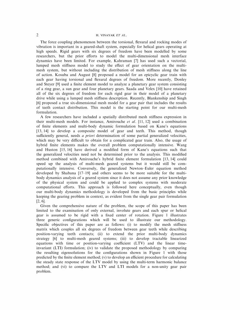
15 show plots of Y1 and u1z when the shaft speed V* is reduced to 24·6 Hz and the

damping proportionality constant cd is decreased to 0·000 01. At this speed, the firstgear mesh frequency fm is equal to the first gear mesh natural frequency (0658 Hzfrom Table 2). Observe that the sidebands around fm , 2fm and 3fm do not seem to matchbetween the predictions of the harmonic balance and numerical integration methods.This is due to an insufficient frequency resolution while calculating the Fourier transformof the time domain predictions obtained from numerical integration. Since these arelower than the primary harmonic frequency by at least an order of magnitude, theyhave an insignificant contribution to the overall response which explains why virtuallyidentical time signals are presented by both methods, as evident from Figures 14(c)and 15(c).

6. COMPARISON OF LTV AND LTI MODELS

6.1.

A single non-unity gear pair (configuration 1) is again chosen for a detailed forcedresponse study using both LTI and LTV models. Each model consists of 12 degrees offreedom as shown in Figure 4(a). For this example case, it is assumed that the excitationis only due to the internal mesh force associated with the transmission error and is given

. ET AL.22

by Qijme (t)=Kij

me (t)dijem (t). The transmission error and the contact length variations are

similar to those used in section 5, as shown in Figures 8 and 9. These have been obtainedusing the LDP software [20, 21] which predicts a scalar value of the transmission erroralong the line of action (pij of Figure 2). Since the spur gears are considered in this example,the internal excitation is only along four degrees of freedom (Y1

G , Y2G , u1

Z , u2Z ). For the sake

of brevity, we will, however, study only one response, say translation Y1G , to compare the

LTI and LTV models. In this study, the mean torque on the system is 1356 N-m (1000in-lb) and the speed V* is varied from 1 to 1800 Hz (60–108 000 rpm). A normal modeexpansion technique is used to obtain the forced response of the LTI model. All 12 modesof Table 2 are used and the excitation Qij

me (t)=Kijme (t)dij

em (t) is obtained by taking a meanvalue of G� ij, shown in Figure 8, and by using Kij

m =KijG� ij, where Kij is the scalar meshstiffness per unit length as defined earlier in section 2.3. At each speed, the response qi iscalculated in frequency domain and then the root-mean-square (r.m.s.) value qi

rms isobtained by summing up the response over the frequency range of interest. Then a speedmap qi

rms (V*) is constructed for a given torque load of the system. The multi-termharmonic balance method is used to calculate the response of the LTV system. The shaftspeed is varied from 1 to 1800 Hz and the static transmission error is assumed to beuniform over this range. The response qi is obtained at each speed from the harmonicbalance method and is given as a function of frequency. Further, a root-mean-square valueqi

rms is calculated at each speed by summing up all of the frequency components of the

Figure 11. Rotational displacement (u1z ) predictions for configuration 1 with shaft speed of 30 Hz. Number

of harmonic terms included in the the harmonic balance method: ns =2, nm =2. (a) Frequency (or order domain)spectrum, (b) cyclic variation or time history, (c) expanded view of (b). Key as in Figure 10.

23

Figure 12. Translational displacement (Y1G ) predictions for configuration 1 with shaft speed of 30 Hz. Number

of harmonic terms included in the harmonic balance method: ns =4, nm =3. (a) Frequency (or order domain)spectrum, (b) cyclic variation or time history, (c) expanded view of (b). Key as in Figure 10.

system variables. Four specific cases, as listed in Table 5, are studied. These cases areconceptually similar to the prior study conducted by Kahraman and Singh [29] for a singleand three-degrees-of-freedom non-linear geared systems of unity gear ratio. Unlike theprevious work, both shaft and gear mesh predictions are considered here in the contextof a 12-degrees-of-freedom linear model of a non-unity gear pair in order to gain animproved understanding of the system behavior over the entire range of operating speed.Only stable, periodic solutions are of interest here.

6.2.

6.2.1. Case IFigure 16(a) shows the speed map of the response Y1

G,rms for a gear pair withharmonically varying transmission error dij

em (t) and the mesh stiffness Kijme (t) for the LTV

model, both containing only the mesh harmonic term such as cos (2pfmt) in equation (38).Of course, the corresponding LTI model has a time-invariant mesh stiffness. It is clear thatfor the LTV model, the excitation force Qij

me (t)=Kijme (t)dij

em (t) of equation (11) is acombination of the two time-varying expressions. A term-by-term product for Qij

me yieldsa term such as cos (2pfmt) cos (2pfmt), which upon simplification gives superharmonicterms cos (4pfmt), cos (6pfmt), etc. In this and subsequent figures, the primary resonantspeed range is from 24 to 54 Hz (1440–3240 rpm) since the mesh harmonic term(cos (2pfmt)) excites the three resonances of the system ( fn2, fn4, fn6) corresponding to Y1

G ,

. ET AL.24

Y2G , uZ . Note that these three natural frequencies coincide with fn1, fn2 and fn3 of the

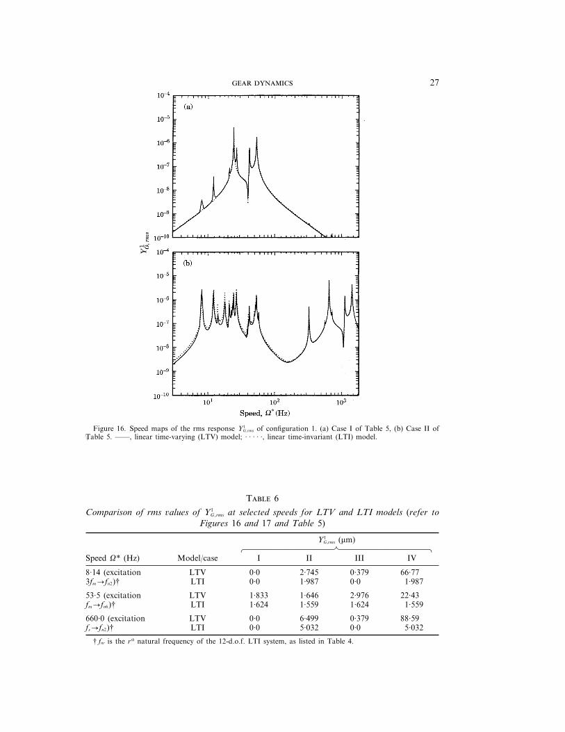
three-degrees of freedom model of Figure 4(b) and Table 2. At speeds below 24 Hz(1440 rpm), superharmonic resonances occur due to the presence of harmonics of the meshfrequency such as terms (cos (4pfmt) and cos (6pfmt) in the excitation as well as the meshstiffness. At speeds above 54 Hz (3240 rpm), subharmonic resonances occur due to thepresence of shaft harmonics (nfs ) which now coincide with the system natural frequencies.For this case, observe that the LTI analysis, as expected, does not exhibit any resonantpeaks in the sub- and superharmonic resonant speed regions. Also, the absence of any shaftfrequency components in the LTV analysis results in a zero response over the subharmonicspeed region. Table 6 lists the r.m.s. value Y1

G,rms at selected resonant speeds for LTI andLTV models. The first speed is V*=8·14 Hz when the third harmonic of the meshexcitation frequency (3fm ) approaches the second natural frequency fn2. Understandably,Y1

G,rms vanishes for the LTI model at this speed as excitation does not contain the 3fm

frequency component. However, the LTV excitation does contain this frequency com-ponent (see Table 5) and consequently a non-zero response is predicted. At a rotationalspeed of V*=53·5 Hz, excitation at the mesh frequency ( fm ) approaches the fourth systemnatural frequency fn4. This component is present in both the LTI and the LTV model, soboth predict non-zero responses. The third rotational speed for comparison, V*=660 Hz,is chosen such that now the shaft frequency ( fs ) approaches fn2. Since the shaft frequency

Figure 13. Rotational displacement (u1z ) predictions for configuration 1 with shaft speed of 30 Hz. Number

of harmonic terms included in the harmonic balance method: ns =4, nm =3. (a) Frequency (or order domain)spectrum, (b) cyclic variation or time history, (c) expanded view of (b). Key as in Figure 10.

25

Figure 14. Translational displacement (Y1G ) predictions for configuration 1 with shaft speed of 24.6 Hz.

Number of harmonic terms included in the harmonic balance method: ns =4, nm =3. (a) Frequency (or orderdomain) spectrum, (b) cyclic variation or time history, (c) expanded view of (b). Key as in Figure 10.

component is not present in either LTI and LTV models, the response vanishes in bothcases.

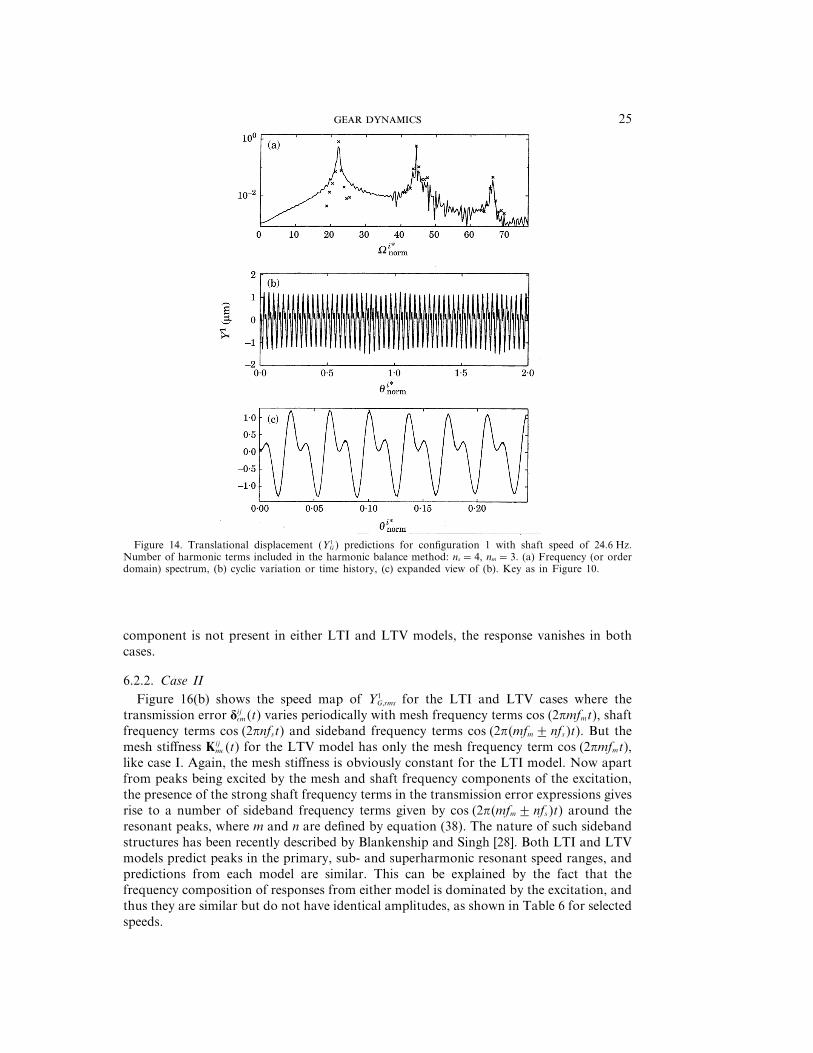
6.2.2. Case IIFigure 16(b) shows the speed map of Y1

G,rms for the LTI and LTV cases where thetransmission error dij

em (t) varies periodically with mesh frequency terms cos (2pmfmt), shaftfrequency terms cos (2pnfst) and sideband frequency terms cos (2p(mfm 2 nfs )t). But themesh stiffness Kij

me (t) for the LTV model has only the mesh frequency term cos (2pmfmt),like case I. Again, the mesh stiffness is obviously constant for the LTI model. Now apartfrom peaks being excited by the mesh and shaft frequency components of the excitation,the presence of the strong shaft frequency terms in the transmission error expressions givesrise to a number of sideband frequency terms given by cos (2p(mfm 2 nfs )t) around theresonant peaks, where m and n are defined by equation (38). The nature of such sidebandstructures has been recently described by Blankenship and Singh [28]. Both LTI and LTVmodels predict peaks in the primary, sub- and superharmonic resonant speed ranges, andpredictions from each model are similar. This can be explained by the fact that thefrequency composition of responses from either model is dominated by the excitation, andthus they are similar but do not have identical amplitudes, as shown in Table 6 for selectedspeeds.

. ET AL.26

Figure 15. Rotational displacement (u1z ) predictions for configuration 1 with shaft speed of 24·6 Hz. Number

of harmonic terms included in the harmonic balance method: ns =4, nm =3. (a) Frequency (or order domain)spectrum, (b) cyclic variation or time history, (c) expanded view of (b). Key as in Figure 10.

6.2.3. Case IIIFigure 17(a) shows the speed map of Y1

G,rms for a case where the transmission error dijem (t)

contains only one frequency term as in case I. But the stiffness Kijme (t) for the LTV analysis

varies periodically with mesh frequency harmonic terms cos (2pmfmt), shaft frequency

T 5

Example cases used to compare the LTV and LTI models of configuration 1

Response XiG , Yi

G , ZiG , ui

x , uiy , ui

z , i=1, 2dij

em (t) Kijme (t) ZXXXXXXXXCXXXXXXXXV

Case (LTI, LTV) (LTV) LTI LTV

I fm fm fm mfm

Harmonic Harmonic Harmonic Periodic

II nfs , mfm , mfm 2 nfs fm nfs , mfm , mfm 2 nfs nfs , mfm , mfm 2 nfs

Periodic Harmonic Periodic Periodic

III fm nfs , mfm , mfm 2 nfs fm nfs , mfm , mfm 2 nfs

Harmonic Periodic Harmonic Periodic

IV nfs , mfm , mfm 2 nfs nfs , mfm , mfm 2 nfs nfs , mfm , mfm 2 nfs nfs , mfm , mfm 2 nfs

Periodic Periodic Periodic Periodic

27

Figure 16. Speed maps of the rms response Y1G,rms of configuration 1. (a) Case I of Table 5, (b) Case II of

Table 5. ——, linear time-varying (LTV) model; · · · · ·, linear time-invariant (LTI) model.:

T 6

Comparison of rms values of Y1G,rms at selected speeds for LTV and LTI models (refer to

Figures 16 and 17 and Table 5)

Y1G,rms (mm)

ZXXXXXXXXXXCXXXXXXXXXXVSpeed V* (Hz) Model/case I II III IV

8·14 (excitation LTV 0·0 2·745 0·379 66·773fm:fn2)† LTI 0·0 1·987 0·0 1·987

53·5 (excitation LTV 1·833 1·646 2·976 22·43fm:fn6)† LTI 1·624 1·559 1·624 1·559

660·0 (excitation LTV 0·0 6·499 0·379 88·59fs:fn2)† LTI 0·0 5·032 0·0 5·032

† fnr is the rth natural frequency of the 12-d.o.f. LTI system, as listed in Table 4.

. ET AL.28

Figure 17. Speed maps of the rms response Y1G,rms of configuration 1. (a) Case III of Table 5, (b) Case IV of

Table 5. ——, Linear time-varying (LTV) model; · · · · ·, linear time-invariant (LTI) model.

terms cos (2pnfst) and sideband terms cos (2p(mfm 2 nfs )t). Since a constant time-averagedmesh stiffness value is used for the LTI analysis, this case is similar to that of case I andit can be verified by comparing Figures 16(a) and 17(a). However, the LTV analysis nowpredicts peaks in the primary, sub- and superharmonic resonant speed regions, asexplained earlier in this section. Some sidebands are also predicted due to the presence ofboth mesh and shaft frequency components. For this case, the LTI model seems to beinadequate especially at higher speeds.

6.2.4. Case IVFigure 17(b) shows the speed map of Y1

G,rms for the case when both transmission errordij

em (t) and mesh stiffness Kijme (t) vary periodically and have terms corresponding to the

mesh frequency harmonics cos (2pmfmt), shaft frequency harmonics cos (2pnfst) and side-band frequency terms cos (2p(mfm 2 nfs )t). Again, a constant time-averaged mesh stiffnessis used for the LTI model and this case is similar to that of case II as can be verified fromFigures 16(b) and 17(b) and Table 6. It is obvious from these results that over the highspeed ranges (mesh subharmonic regimes) the LTI predictions are accurate. However, the

29

LTI predictions are invariably lower, by as much as two orders of magnitude, than theLTV predictions in the primary and superharmonic resonant speed ranges. This is due tothe fact that at lower speeds, the gear pair exhibits parametric resonances. Also, the LTImodel does not predict those sidebands which are associated with the parametric excitationphenomenon.

7. CONCLUSIONS

The analysis of multi-mesh transmissions is indeed complicated since the effects ofcontact mechanics, rigid body motions, elastic deformations, etc. must be consideredsimultaneously. Obviously, a single paper cannot address all of them in a complete andsatisfying manner. Consequently, this paper should be viewed as a first report on acomprehensive research project. Three main contributions, beyond the prior work [6, 23],emerge which will guide us and other researchers in future work. First, new and usefulextensions to the multi-body dynamics framework have been developed which are suitableand yet computationally efficient for multi-mesh geared systems. Second, the strategy ofconstructing steady state periodic solutions to the resulting linear position or time-varying(LTV) formulations by using the multi-term harmonic balance is very promising; theseinclude both low (shaft) and high (mesh) frequency terms. Third, new results for anon-unity gear pair have been generated by using LTI and LTV models, including ageneralized natural frequency graph and r.m.s. response versus speed maps. Both sidebandstructures and sub- and superharmonic resonant regimes have been predicted successfully.Various simplifications and approximations seem to be valid since analytical predictionsmatch well with those yielded by the commonly used numerical solvers such as the finiteelement method and the direct time domain integration. Ongoing research is focused onthe inclusion of elastic characteristics of gear blanks. Subsequently, components of theplanetary gear drives will be modelled. Parallel efforts will also be directed towards anexperimental validation of the methodology.

ACKNOWLEDGMENT

This research has been supported by Army Research Office (URI Grant DAAL03-92-G-0120; 1992–97; project monitor Dr T. L. Doligalski).

REFERENCES

1. H. O and D. R. H 1988 Journal of Sound and Vibration 121, 83–411. Mathematicalmodels used in gear dynamics – a review.

2. G. W. B and R. S 1992 American Society of Mechanical Engineers, Proceedingsof Sixth International Power Transmission and Gearing Conference, DE 43-1, 137–146. Acomparative study of selected gear mesh interface dynamic models.

3. H. I and A. T 1984 Proceedings of Vibration in Rotating Machinery, 67–72. Instituteof Mechanical Engineers. Coupled torsional-flexural vibration of a shaft in a geared system.

4. H. I, A. T and H. Y 1986 Bulletin of the Japan Society of MechanicalEngineers 29(252), 1811–1816. Dynamic characteristics of a gear train system with softlysupported shafts.

5. J. W. D and L. D. M 1985 American Society of Mechanical Engineers, paper no.85-DET-11. Linear dynamic coupling in geared rotor systems.

6. G. W. B and R. S 1995 Mechanism and Machine Theory. 30, 43–57.A new gear interface dynamic model to predict multi-dimensional force coupling andexcitation.

. ET AL.30

7. A K 1992 American Society of Mechanical Engineers, Proceedings of Sixth InternationalPower Transmission and Gearing Conference, DE 43-1, 365–373. Dynamic analysis of amulti-mesh helical gear train.

8. R. K and R. A 1984 American Society of Mechanical Engineers, Paper no.84-DET-229. Gear mesh stiffness and load sharing in planetary gearing.

9. M. G. D and G. C. S 1992 American Society of Mechanical Engineers, Proceedingsof Sixth International Power Transmission and Gearing Conference, DE 43-1, 117–127. Dynamicanalysis of planetary gear system.

10. A. S and P. V 1992 American Society of Mechanical Engineers, Proceedings of SixthInternational Power Transmission and Gearing Conference, 43-2, 513–520. An extended model forthe analysis of the dynamic behavior of planetary trains.

11. F. M. L. A, N. H. S and M. X 1991 Machinery Dynamics and ElementVibrations, DE-vol. 36, 257–262. Dynamic analysis of flexible gear trains/transmissions: anautomated approach.

12. F. M. L. A 1992 Computational Methods in Multibody Dynamics. Englewood Cliffs,New Jersey: Prentice Hall.

13. T. R. K and D. A. L 1980 Journal of Guidance and Control 3(2), 99–112. Formulationof equation of motion for complex spacecraft.

14. T. R. K and D. A. L 1983 Journal of Applied Mechanics 50, 1071–1079. MultibodyDynamics.

15. J. T. W and R. L. H 1988 Computers and Structures, 29(2), 331–338. Computationalmethods in constrained Multibody dynamics: matrix formulism.

16. J. T. W 1990 Transaction of the American Society of Mechanical Engineers, Journal of AppliedMechanics 57, 750–757. Inverse dynamics of constrained multibody systems.

17. A. A. S 1985 American Society of Mechanical Engineers, Journal of Vibration, Acoustics,Stress, and Reliability in Design 107, 431–439. Automated analysis of constrained systems of rigidand flexible bodies.

18. A. A. S 1990 Transactions of the American Society of Mechanical Engineers, Journal ofApplied Mechanics 112, 496–503. Dynamics of flexible bodies using generalized Newton–Eulerequations.

19. A. A. S 1989 Dynamics of Multibody Systems. New York: John Wiley.20. Load Distribution Program (LDP), ver. 8.2, 1993 Gear Dynamics and Gear Noise Research

Laboratory, Ohio State University.21. D. R. H 1990 Gear Design, Manufacturing and Inspection Manual, Society of Automotive

Engineering AE-15, 213–222. Gear noise source and their prediction using mathematical models.22. ANSYS, ver. 5.0, 1993 Swanson Analysis Systems Inc., Houston, Pennsylvania.23. G. W. B and R. S 1995 Mechanism and Machine Theory 30, 323–339. Dynamic

force transmissibility in helical gear pairs.24. A. K and R. S 1991 Journal of Sound and Vibration 149, 495–498. Error associated

with a reduced order linear model of a spur gear pair.25. M. R. L, C. P and R. S 1995 ASME Journal of Dynamic Systems,

Measurement and Control. Dynamic analysis of Brushless D.C. motor using a modified harmonicbalance method. (in press).

26. T. R and R. S 1995 Journal of Sound and Vibration 182, 303–322. Dynamic analysisof a reverse-idler gear pair with concurrent clearances.

27. A. G 1981 Kronecker Products and Matrix Calculus. New York: John Wiley.28. G. W. B and R. S 1995 Journal of Sound and Vibration 179, 13–36. Analytical

solution for modulation sidebands associated with a class of mechanical oscillators.29. A. K and R. S 1991 Journal of Sound and Vibration 146, 153–156. Interactions

between time-varying mesh stiffness and clearance non-linearities in a geared system.30. M. U and A. R 1966 Journal of Mathematical Analysis and Applications 14, 107–140.

Numerical computation of nonlinear forced oscillations by Galerkin’s procedure.

APPENDIX A: LIST OF SYMBOLS

A rotational transformation matrixA cross-section area of shaftsa, b , c, d , e Fourier coefficient vectorsa, b shaft lengthsC damping matrix

31

cd damping proportionality constantE Young’s modulusF force vectorF discrete Fourier transform (DFT) matricesf frequency (Hz)fn natural frequency (Hz)G Euler parameter matrixh contact line offsetI identity matrixi, j gear numberK scalar stiffness valueK stiffness matrixD Fourier differentiation matrixM inertia matrixm inertia sub-matricesm, n harmonic ordermg gear speed ratioNG number of gearsn bearing position vectorP a point in the line of contactp net transmission errorQ generalized force vectorq generalized co-ordinate vectorR generalized translational co-ordinateR residuer vector position of a point in the geometric co-ordinateT torque vectort timeu vector position of a point in the geometric co-ordinates with respect to the pitch pointu, v, w, p, q unit vectors along the mesh co-ordinatesX state space system variableX, Y, Z co-ordinate systemG contact lengthd displacementd small changez shaft subspaceU damping matrixu genearlized rotational co-ordinateu nominal angular positionm mesh spacen subharmonic indexJ system matrixj gear diameter ratior densityt non-dimensionalized timeF mean square normfi gear diameterx, g, f mesh co-ordinate systemx, s, h helical mesh co-ordinate systemC helix angleV rotational speed (rpm or Hz)vnr natural frequency (rad/s)

Subscripts

T transposei, j gear numbersp order of differentiation* nominal value�−1� term-by-term inverse

. ET AL.32

Subscripts

b baseG body co-ordinate systemg rigid body blank motionGm geometric co-ordinate systemk bearing numberm dynamicmd dynamic (dissipative)me dynamic (elastic)o meanq generalized co-ordinatesR linears shaftsB shaft bendingsR shaft rockingsT shaft longitudinalb bearingr modal indexrms root mean squarex, y, z co-ordinatesu angulare transmission errors linear position along the line of contact0 asymmetric matrix

AbbreviationsFEM finite element methodLTI linear time-invariantLTV linear time varyingSTE static transmission errordiag diagonal matrixvec vectorize