linear elastic waves (cambridge texts in applied mathematics) (john g. harris) 0521643686
TRANSCRIPT

8/4/2019 Linear Elastic Waves (Cambridge Texts in Applied Mathematics) (John G. Harris) 0521643686
http://slidepdf.com/reader/full/linear-elastic-waves-cambridge-texts-in-applied-mathematics-john-g-harris 1/180

8/4/2019 Linear Elastic Waves (Cambridge Texts in Applied Mathematics) (John G. Harris) 0521643686
http://slidepdf.com/reader/full/linear-elastic-waves-cambridge-texts-in-applied-mathematics-john-g-harris 2/180
This page intentionally left blank

8/4/2019 Linear Elastic Waves (Cambridge Texts in Applied Mathematics) (John G. Harris) 0521643686
http://slidepdf.com/reader/full/linear-elastic-waves-cambridge-texts-in-applied-mathematics-john-g-harris 3/180
Linear Elastic Waves
Wave propagation and scattering are among the most fundamental processesthat we use to comprehend the world around us. Whereas these processes areoften very complex, one way to begin to understand them is to study wave prop-agation in the linear approximation. This is a book describing such propagationusing, as a context, the equations of elasticity. Two unifying themes are used.
The rst is that an understanding of plane wave interactions is fundamental tounderstanding more complex wave interactions. The second is that waves arebest understood in an asymptotic approximation where they are free of the com-plications of their excitation and are governed primarily by their propagationenvironments. The topics covered include reection, refraction, propagation of interfacial waves, integral representations, radiation and diffraction, and prop-agation in closed and open waveguides.
Linear Elastic Wavesis an advanced level textbook directed at applied mathe-maticians, seismologists, and engineers.
John G. Harris received an undergraduate degree (honors) in 1971 from McGillUniversity, where he studied electrical engineering and gained a lasting interestin wave propagation. In 1979, he received a doctoral degree in applied mathe-matics from Northwestern University for a thesis on elastic-wave diffractionproblems. Following this, he joined the Theoretical and Applied Mechan-ics Department at the University of Illinois (Urbana-Champaign), where heteaches dynamics and mathematical methods and carries out research on elastic-wave problems at microwave frequencies. He has used asymptotic methods of analysis to explore diffraction and imaging, propagation and scattering of interfacial waves, and waveguiding.

8/4/2019 Linear Elastic Waves (Cambridge Texts in Applied Mathematics) (John G. Harris) 0521643686
http://slidepdf.com/reader/full/linear-elastic-waves-cambridge-texts-in-applied-mathematics-john-g-harris 4/180

8/4/2019 Linear Elastic Waves (Cambridge Texts in Applied Mathematics) (John G. Harris) 0521643686
http://slidepdf.com/reader/full/linear-elastic-waves-cambridge-texts-in-applied-mathematics-john-g-harris 5/180
Cambridge Texts in Applied Mathematics
Maximum and Minimum PrinciplesM. J. S EWELL
SolitonsP. G. D RAZIN AND R. S. J OHNSON
The Kinematics of MixingJ. M. O TTINO
Introduction to Numerical Linear Algebra and Optimisation
PHILIPPE G. C IARLETIntegral Equations
DAVID PORTER AND DAVID S. G. S TIRLING
Perturbation MethodsE. J. H INCH
The Thermomechanics of Plasticity and FractureGERARD A. M AUGIN
Boundary Integral and Singularity Methods for Linearized Viscous FlowC. P OZRIKIDIS
Nonlinear Wave Processes in AcousticsK. N AUGOLNYKH AND L. OSTROVSKY
Nonlinear SystemsP. G. D RAZIN
Stability, Instability and ChaosPAUL GLENDINNING
Applied Analysis of the Navier–Stokes EquationsC. R. D OERING AND J. D. G IBBON
Viscous FlowH. O CKENDON AND J. R. O CKENDON
Scaling, Self-Similarity, and Intermediate AsymptoticsG. I. B ARENBLATT
A First Course in the Numerical Analysis of Differential EquationsARIEH ISERLES
Complex Variables: Introduction and ApplicationsMARK J. ABLOWITZ AND ATHANASSIOS S. F OKAS
Mathematical Models in the Applied SciencesA. C. F OWLER
Thinking About Ordinary Differential EquationsROBERT E. O’M ALLEY
A Modern Introduction to the Mathematical Theory of Water WavesR. S. J OHNSON
Rareed Gas DynamicsCARLO CERCIGNANI
Symmetry Methods for Differential EquationsPETER E. H YDON
High Speed FlowC. J. C HAPMAN
Wave MotionJ. B ILLINGHAM AND A. C. K ING
An Introduction to MagnetohydrodynamicsP. A. D AVIDSON
Linear Elastic WavesJOHN G. H ARRIS

8/4/2019 Linear Elastic Waves (Cambridge Texts in Applied Mathematics) (John G. Harris) 0521643686
http://slidepdf.com/reader/full/linear-elastic-waves-cambridge-texts-in-applied-mathematics-john-g-harris 6/180

8/4/2019 Linear Elastic Waves (Cambridge Texts in Applied Mathematics) (John G. Harris) 0521643686
http://slidepdf.com/reader/full/linear-elastic-waves-cambridge-texts-in-applied-mathematics-john-g-harris 7/180
Linear Elastic Waves
JOHN G. HARRIS
University of Illinois at Urbana-Champaign

8/4/2019 Linear Elastic Waves (Cambridge Texts in Applied Mathematics) (John G. Harris) 0521643686
http://slidepdf.com/reader/full/linear-elastic-waves-cambridge-texts-in-applied-mathematics-john-g-harris 8/180
The Pitt Building, Trumpington Street, Cambridge, United Kingdom
The Edinburgh Building, Cambridge CB2 2RU, UK 40 West 20th Street, New York, NY 10011-4211, USA 477 Williamstown Road, Port Melbourne, VIC 3207, AustraliaRuiz de Alarcón 13, 28014 Madrid, SpainDock House, The Waterfront, Cape Town 8001, South Africa
http://www.cambridge.org
First published in printed format
ISBN 0-521-64368-6 hardback ISBN 0-521-64383-X paperback
ISBN 0-511-04041-5 eBook
Cambridge University Press 2004
2001
(netLibrary)
©

8/4/2019 Linear Elastic Waves (Cambridge Texts in Applied Mathematics) (John G. Harris) 0521643686
http://slidepdf.com/reader/full/linear-elastic-waves-cambridge-texts-in-applied-mathematics-john-g-harris 9/180
To Beatriz

8/4/2019 Linear Elastic Waves (Cambridge Texts in Applied Mathematics) (John G. Harris) 0521643686
http://slidepdf.com/reader/full/linear-elastic-waves-cambridge-texts-in-applied-mathematics-john-g-harris 10/180

8/4/2019 Linear Elastic Waves (Cambridge Texts in Applied Mathematics) (John G. Harris) 0521643686
http://slidepdf.com/reader/full/linear-elastic-waves-cambridge-texts-in-applied-mathematics-john-g-harris 11/180
Contents
Preface page xiii
1 Simple Wave Solutions 11.1 Model Equations 1
1.1.1 One-Dimensional Models 31.1.2 Two-Dimensional Models 41.1.3 Displacement Potentials 51.1.4 Energy Relations 5
1.2 The Fourier and Laplace Transforms 61.3 A Wave Is Not a Vibration 111.4 Dispersive Propagation 13
1.4.1 An Isolated Interaction 131.4.2 Periodic Structures 15
References 18
2 Kinematical Descriptions of Waves 202.1 Time-Dependent Plane Waves 202.2 Time-Harmonic Plane Waves 222.3 Plane-Wave or Angular-Spectrum Representations 24
2.3.1 A Gaussian Beam 242.3.2 An Angular-Spectrum Representation of a
Spherical Wave 262.3.3 An Angular-Spectrum Representation of a
Cylindrical Wave 282.4 Asymptotic Ray Expansion 28
2.4.1 Compressional Wave 292.4.2 Shear Wave 33
ix

8/4/2019 Linear Elastic Waves (Cambridge Texts in Applied Mathematics) (John G. Harris) 0521643686
http://slidepdf.com/reader/full/linear-elastic-waves-cambridge-texts-in-applied-mathematics-john-g-harris 12/180
x Contents
Appendix: Spherical and Cylindrical Waves 34References 35
3 Reection, Refraction, and Interfacial Waves 373.1 Reection of a Compressional Plane Wave 37
3.1.1 Phase Matching 393.1.2 Reection Coefcients 40
3.2 Reection and Refraction 413.3 Critical Refraction and Interfacial Waves 443.4 The Rayleigh Wave 48
3.4.1 The Time-Harmonic Wave 493.4.2 Transient Wave 503.4.3 The Rayleigh Function 513.4.4 Branch Cuts 52
References 55
4 Green’s Tensor and Integral Representations 564.1 Introduction 564.2 Reciprocity 574.3 Green’s Tensor 58
4.3.1 Notes 614.4 Principle of Limiting Absorption 624.5 Integral Representation: A Source Problem 64
4.5.1 Notes 654.6 Integral Representation: A Scattering Problem 65
4.6.1 Notes 664.7 Uniqueness in an Unbounded Region 68
4.7.1 No Edges 684.7.2 Edge Conditions 694.7.3 An Inner Expansion 71
4.8 Scattering from an Elastic Inclusion in a Fluid 72References 76
5 Radiation and Diffraction 775.1 Antiplane Radiation into a Half-Space 77
5.1.1 The Transforms 785.1.2 Inversion 79
5.2 Buried Harmonic Line of Compression I 825.3 Asymptotic Approximation of Integrals 86

8/4/2019 Linear Elastic Waves (Cambridge Texts in Applied Mathematics) (John G. Harris) 0521643686
http://slidepdf.com/reader/full/linear-elastic-waves-cambridge-texts-in-applied-mathematics-john-g-harris 13/180
Contents xi
5.3.1 Watson’s Lemma 875.3.2 Method of Steepest Descents 90
5.3.3 Stationary Phase Approximation 945.4 Buried Harmonic Line of Compression II 965.4.1 The Complex Plane 965.4.2 The Scattered Compressional Wave 985.4.3 The Scattered Shear Wave 99
5.5 Diffraction of an Antiplane Shear Wave at an Edge 1015.5.1 Formulation 1025.5.2 Wiener–Hopf Solution 1045.5.3 Description of the Scattered Waveeld 108
5.6 Matched Asymptotic Expansion Study 112Appendix: The Fresnel Integral 116References 119
6 Guided Waves and Dispersion 1216.1 Harmonic Waves in a Closed Waveguide 121
6.1.1 Partial Waves and the Transverse Resonance Principle 1236.1.2 Dispersion Relation: A Closed Waveguide 124
6.2 Harmonic Waves in an Open Waveguide 1286.2.1 Partial Wave Analysis 1296.2.2 Dispersion Relation: An Open Waveguide 131
6.3 Excitation of a Closed Waveguide 1346.3.1 Harmonic Excitation 1346.3.2 Transient Excitation 135
6.4 Harmonically Excited Waves in an Open Waveguide 1396.4.1 The Waveeld in the Layer 1406.4.2 The Waveeld in the Half-Space 1456.4.3 Leaky Waves 146
6.5 A Laterally Inhomogeneous, Closed Waveguide 1466.6 Dispersion and Group Velocity 150
6.6.1 Causes of Dispersion 1506.6.2 The Propagation of Information 1516.6.3 The Propagation of Angular Frequencies 153
References 157
Index 159

8/4/2019 Linear Elastic Waves (Cambridge Texts in Applied Mathematics) (John G. Harris) 0521643686
http://slidepdf.com/reader/full/linear-elastic-waves-cambridge-texts-in-applied-mathematics-john-g-harris 14/180

8/4/2019 Linear Elastic Waves (Cambridge Texts in Applied Mathematics) (John G. Harris) 0521643686
http://slidepdf.com/reader/full/linear-elastic-waves-cambridge-texts-in-applied-mathematics-john-g-harris 15/180
Preface
A wavebuilds upperhaps it says its name, I don’t understand,mutters, humps its load
of movement and foamand withdraws. Whocan I ask what it said to me? 1
Wave propagation and scattering are among the most fundamental processesthat we use to comprehend the world around us. While these processes areoften very complex, one way to begin to understand them is to study linear
wave propagation. This is a book describing such propagation.I use the equations of linear elasticity to form a context for my description of
wave propagation. However, the reader’s knowledge of elasticity need not bevery great, and experience with a related eld theory, such as uid mechanics orelectromagnetic theory, is sufcient to understand what is written here. In manyplaces I treat only the antiplane shear problem because I do not believe that theextra work needed to do the analogous inplane problem adds anything of signi-
cance to understanding the underlying wave processes. Nevertheless, wherean inplane elastic problem introduces a unique feature, such as the presence of a nondispersive surface wave, that problem is treated.
This is also a book describing the parts of applied mathematics that de-scribe the propagation and scattering of linear elastic waves. It assumes that thereader has a good background in calculus, differential equations, and complexanalysis. By this I mean that the reader should have studied most of the topics in
1 Neruda, Pablo, Soliloquy in the Waves , pp. 185–186. In Isla Negra, a Notebook , translated byA. Reid. New York: Noonday Press. 1981.
xiii

8/4/2019 Linear Elastic Waves (Cambridge Texts in Applied Mathematics) (John G. Harris) 0521643686
http://slidepdf.com/reader/full/linear-elastic-waves-cambridge-texts-in-applied-mathematics-john-g-harris 16/180
xiv Preface
Courant and John, Introduction to Calculus and Analysis , Vols. 1 and 2 (1989)and in Boyce and DiPrima, Elementary Differential Equations and BoundaryValue Problems
(1992). Moreover, the reader should be able to look thingsup in Carrier, Krook, and Pearson, Functions of a Complex Variable (1983) orAblowitz and Fokas Complex Variables , Introduction and Applications (1997)and Zauderer Partial Differential Equations of Applied Mathematics (1998)and not feel lost. None of the mathematical analyses exceed, in sophistica-tion or difculty, those found in Courant and John (1989). I work almostentirely in Cartesian coordinates so that no knowledge of special functions orthe transforms associated with them is needed. Some previous experience withasymptotic analysis would be helpful, but is not essential. All the asymptoticanalysis needed is explained in the book.
I have used two unifying themes throughout. The rst is that an understand-ing of plane-wave interactions is fundamental to understanding more complexwave interactions. The second is that waves are best understood in an asymp-totic approximation where they are free of the complications of their excitationand are governed primarily by their propagation environment. Therefore plane-wave spectral analyses and asymptotic approximations are the main techniquesused to study the more complicated problems.
The selection of problems for the reader is small and directed at engaginghim or her in the development of the subject. The problems are an integral partof the book and most should be attempted.
I have tried to avoid a menagerie of symbols. In general I use Cartesian ten-sors such as τ i j , where the indices i , j = 1, 2, 3, or a boldface notation τ . Thesymbol ∂i is used to represent the partial derivative with respect to the i th coor-dinate. Similarly, sometimes I use d x f to represent d f / dx . Repeated indicesare summed over 1, 2, 3 unless otherwise indicated. For problems engagingonly two coordinates, subscripts using Greek letters such as α, β = 1, 2 areused so that a vector component would be written as u β and a partial deriva-tive as ∂α . When these subscripts are repeated they are summed over 1, 2. Attimes I use symbols such as c L or cT when there is need to distinguish betweenparameters that relate to compressional or shear disturbances, but when thatdistinction is not important I drop the subscript. Constants such as A are usedover and over again and have no special meaning.
Professor Jan Achenbach was my research advisor. He taught me the subject.His inuence is everywhere is this book. I thank him. I have been supportedover the years primarily by the National Science Foundation, though recentlyalso by the Air Force Ofce of Scientic Research. I am very grateful fortheir support. Elaine Wilson typed the early parts of this manuscript and Mike

8/4/2019 Linear Elastic Waves (Cambridge Texts in Applied Mathematics) (John G. Harris) 0521643686
http://slidepdf.com/reader/full/linear-elastic-waves-cambridge-texts-in-applied-mathematics-john-g-harris 17/180
Preface xv
Greenberg provided the illustrations. Don Carlson and Bill Phillips toleratedmy complaints with humor; Eduardo Velasco prevented me from publishing a
discussion of group velocity that was at best muddled. To everyone, thank you.The book undoubtedly contains errors, for which I alone am responsible. Ianticipate that few if any are serious.
Books Cited
Ablowitz, M. J. and Fokas, A. S. 1997. Complex Variables, Introduction and Applications. New York: Cambridge.
Boyce, W. E. and DiPrima, R. C. 1992. Elementary Differential Equations and Boundary Value Problems, 5th ed. New York: Wiley.
Carrier, G. F., Krook, M., and Pearson, C. E. 1983. Functions of a Complex Variable.Ithaca, NY: Hod Books.
Courant, R. and John, F. 1989. Introduction to Calculus and Analysis , Vols. 1 and 2.New York: Springer.
Zauderer, E. 1983. Partial Differential Equations of Applied Mathematics. New York:Wiley-Interscience.
Evanston and Urbana, Summer 2000.

8/4/2019 Linear Elastic Waves (Cambridge Texts in Applied Mathematics) (John G. Harris) 0521643686
http://slidepdf.com/reader/full/linear-elastic-waves-cambridge-texts-in-applied-mathematics-john-g-harris 18/180

8/4/2019 Linear Elastic Waves (Cambridge Texts in Applied Mathematics) (John G. Harris) 0521643686
http://slidepdf.com/reader/full/linear-elastic-waves-cambridge-texts-in-applied-mathematics-john-g-harris 19/180
1
Simple Wave Solutions
Synopsis
Chapter 1 provides the background, both the model equations and some of the mathematical transformations, needed to understand linear elastic waves.Only the basic equations are summarized, without derivation. Both Fourier
and Laplace transforms and their inverses are introduced and important signconventions settled. The Poisson summation formula is also introduced andused to distinguish between a propagating wave and a vibration of a boundedbody.
A linear wave carries information at a particular velocity, the group velocity,which is characteristic of the propagation structure or environment. It is thistransmitting of information that gives linear waves their special importance.
In order to introduce this aspect of wave propagation, propagation in one-dimensional periodic structures is discussed. Such structures are dispersive andtherefore transmit information at a speed different from the wavespeed of theirindividual components.
1.1 Model Equations
The equations of linear elasticity consist of (1) the conservation of linear andangular momentum, and (2) a constitutive relation relating force and deforma-tion. In the linear approximation density ρ is constant. The conservation of mechanical energy follows from (1) and (2). The most important feature of themodel is that the force exerted across a surface, oriented by the unit normal n j ,by one part of a material on the other is given by the traction t i = τ j i n j , whereτ j i is the stress tensor. The conservation of angular momentum makes the stress
tensor symmetric; that is, τ i j = τ j i . The conservation of linear momentum, in
1

8/4/2019 Linear Elastic Waves (Cambridge Texts in Applied Mathematics) (John G. Harris) 0521643686
http://slidepdf.com/reader/full/linear-elastic-waves-cambridge-texts-in-applied-mathematics-john-g-harris 20/180
2 1 Simple Wave Solutions
differential form, is expressed as
∂k τ ki + ρ f i = ρ∂ t ∂t u i . (1.1)
The term f is a force per unit mass.Deformation is described by using a strain tensor,
i j = (∂i u j + ∂ j u i )/ 2, (1.2)
where u i is ith component of particle displacement. The symmetrical denition
of the deformation ensures that no rigid-body rotations are included. However,the underlying dependence of the deformation is upon the ∇ u . For a homoge-neous, isotropic, linearly elastic solid, stress and strain are related by
τ i j = λ kk δi j + 2µ i j , (1.3)
where λ and µ are Lam e’s elastic constants. Substituting (1.2) in (1.3), followedby substituting the outcome into (1.1), gives one form of the equation of motion,namely
(λ + µ )∂i ∂k u k + µ∂ j ∂ j u i + ρ f i = ρ∂ t ∂t u i . (1.4)
Written in vector notation, the equation becomes
(λ + µ )∇ (∇ · u) + µ ∇ 2u + ρ f = ρ∂ t ∂t u . (1.5)
When the identity ∇2u = ∇ (∇ · u ) − ∇ ∧ ∇ ∧ u is used, the equation can also
be written in the form
(λ + 2µ )∇ (∇ · u ) − µ ∇ ∧ ∇ ∧ u + ρ f = ρ∂ t ∂t u . (1.6)
This last equation indicates that elastic waves have both dilitational ∇ · u androtational ∇ ∧ u deformations.
If ∂ R is the boundary of a region R occupied by a solid, then commonly t and u are prescribed on ∂ R . When t is given over part of ∂ R and u overanother part, the boundary conditions are said to be mixed. One very commonboundary condition is to ask that t = 0 everywhere on ∂ R . This models thecase in which a solid surface is adjacent to a gas of such small density andcompressibility that it is almost a vacuum. When R is innite in one or moredimensions, special conditions are imposed such that a disturbance decays tozero at innity or radiates outward toward innity from any sources containedwithin R .

8/4/2019 Linear Elastic Waves (Cambridge Texts in Applied Mathematics) (John G. Harris) 0521643686
http://slidepdf.com/reader/full/linear-elastic-waves-cambridge-texts-in-applied-mathematics-john-g-harris 21/180
1.1 Model Equations 3
Another common situation is that in which ∂ R 12 is the boundary betweentwo regions, 1 and 2, occupied by solids having different properties. Contact
between solid bodies is quite complicated, but in many cases it is usual toassume that the traction and displacement, t and u , are continuous. This modelswelded contact. One other simple continuity condition that commonly arisesis that between a solid and an ideal uid. Because the viscosity is ignored, thetangential component of t is set to zero, while the normal component of tractionand the normal component of displacement are made continuous.
These are only models and are often inadequate. To briey indicate someof the possible complications, consider two solid bodies pressed together. A(linear) wave incident on such a boundary would experience continuity of trac-tion and displacement when the solids press together, but would experience atraction-free boundary condition when they pull apart (Comninou and Dundurs,1977). This produces a complex nonlinear interaction.
The reader may consult Hudson (1980) for a succinct discussion of linearelasticity or Atkin and Fox (1980) for a somewhat more general view.
1.1.1 One-Dimensional Models
We assume that the various waveeld quantities depend only on the variables x1 and t . For longitudinal strain , u 1 is nite, while u 2 and u 3 are assumed to bezero, so that (1.2) combined with (1.3) becomes
τ 11 = (λ + 2µ )∂1u 1 , τ 22 = τ 33 = λ∂ 1u 1 , (1.7)
and (1.1) becomes
(λ + 2µ )∂1∂1u 1 + ρ f 1 = ρ∂ t ∂t u 1 . (1.8)
For longitudinal stress , all the stress components except τ 11 are assumed to bezero. Now (1.3) becomes
τ 11 = E ∂1u 1 , E = µ 3λ + 2µλ + µ
, (1.9)
and
∂2u 2 = ∂3u 3 = − ν∂ 1u 1 , ν =λ
2(λ + µ ). (1.10)
Now (1.1) becomes
E ∂1∂1u 1 + ρ f 1 = ρ∂ t ∂t u 1 . (1.11)

8/4/2019 Linear Elastic Waves (Cambridge Texts in Applied Mathematics) (John G. Harris) 0521643686
http://slidepdf.com/reader/full/linear-elastic-waves-cambridge-texts-in-applied-mathematics-john-g-harris 22/180
4 1 Simple Wave Solutions
Note that (1.8) and (1.11) are essentially the same, though they have somewhatdifferent physical meanings. The longitudinal stress model is useful for rodshaving a small cross section and a traction-free surface. Stress components thatvanish at the surface are assumed to be negligible in the interior.
1.1.2 Two-Dimensional Models
Let us assume that the various waveeld quantities are independent of x3 . As aconsequence, (1.1) breaks into two separate equations, namely
∂β τ β 3 + ρ f 3 = ρ∂ t ∂t u 3 , (1.12)
∂β τ βα + ρ f α = ρ∂ t ∂t u α . (1.13)
Greek subscripts α, β = 1, 2 are used to indicate that the independent spatialvariables are x1 and x2 . The case for which the only nonzero displacementcomponent is u 3( x1 , x2 , t ), namely (1.12), is called antiplane shear motion, orSH motion for shear horizontal.
τ 3β = µ∂ β u 3 , (1.14)
giving, from (1.12),
µ∂ β ∂β u 3 + ρ f 3 = ρ∂ t ∂t u 3 . (1.15)
Note that this is a two-dimensional scalar equation, similar to (1.8) or (1.11).
The case for which u 3 = 0, while the other two displacement componentsare generally nonzero, (1.13), is called inplane motion . The initials P and SVare used to describe the two types of inplane motion, namely compressionaland shear vertical, respectively. For this case (1.3) becomes
τ αβ = λ∂ γ u γ δαβ + µ (∂α u β + ∂β u α ), (1.16)
and
τ 33 = λ∂ γ u γ . (1.17)
The equation of motion remains (1.4); that is,
(λ + µ )∂α ∂β u β + µ∂ β ∂β u α + ρ f α = ρ∂ t ∂t u α . (1.18)
This last equation is a vector equation and contains two wave types, compres-sional and shear, whose character we explore shortly. It leads to problems of some complexity.

8/4/2019 Linear Elastic Waves (Cambridge Texts in Applied Mathematics) (John G. Harris) 0521643686
http://slidepdf.com/reader/full/linear-elastic-waves-cambridge-texts-in-applied-mathematics-john-g-harris 23/180
1.1 Model Equations 5
These two-dimensional equations are the principal models used. The scalarmodel, (1.14), allows us to solve complicated problems in detail without being
overwhelmed by the size and length of the calculations needed, while the vectormodel, (1.18), allows us enough structure to indicate the complexity found inelastic-wave propagation.
1.1.3 Displacement Potentials
When (1.4)–(1.6) are used, a boundary condition, such as t = 0, is relativelyeasy to implement. However, in problems in which there are few boundary con-ditions, it is often easier to cast the equations of motion into a simpler form andallow the boundary condition to become more complicated. One way to do thisis to use the Helmholtz theorem (Phillips, 1933; Gregory, 1996) to express theparticle displacement u as the sum of a scalar ϕ and a vector potential ψ ; that is,
u = ∇ ϕ + ∇ ∧ ψ , ∇ · ψ = 0. (1.19)
The second condition is needed because u has only three components (the parti-cular condition selected is not the only possibility). Assume f = 0. Substitutingthese expressions into (1.6) gives
(λ + 2µ )∇ ∇2ϕ − 1/ c2
L ∂t ∂t ϕ + µ ∇ ∧ ∇2ψ − 1/ c2
T ∂t ∂t ψ = 0.
(1.20)
The equation can be satised if
∇2ϕ = 1/ c2
L ∂t ∂t ϕ, c2 L = (λ + 2µ )/ρ, (1.21)
∇2ψ = 1/ c2
T ∂t ∂t ψ , c2T = µ/ρ. (1.22)
The terms c L and cT are the compressional or longitudinal wavespeed, and shearor transverse wavespeed, respectively. The scalar potential describes a wave of compressional motion, which in the plane-wave case is longitudinal, while thevector potential describes a wave of shear motion, which in the plane-wavecase is transverse. Knowing ϕ and ψ , do we know u completely? Yes we do.Proofs of completeness, along with related references, are given in Achenbach(1973).
1.1.4 Energy Relations
The remaining conservation law of importance is the conservation of mecha-nical energy. Again assume f = 0. This law can be derived directly from

8/4/2019 Linear Elastic Waves (Cambridge Texts in Applied Mathematics) (John G. Harris) 0521643686
http://slidepdf.com/reader/full/linear-elastic-waves-cambridge-texts-in-applied-mathematics-john-g-harris 24/180
6 1 Simple Wave Solutions
(1.1)–(1.3) by taking the dot product of ∂t u with (1.1). This gives, initially,
∂ j τ j i ∂t u i − ρ (∂t ∂t u i )∂t u i = 0. (1.23)
Forming the product τ kl kl , using (1.3), and making use of the decomposition∂ j u i = j i + ω j i , where ω j i = (∂ j u i − ∂i u j )/ 2, allows us to write (1.23) as
12 ∂t (ρ∂ t u i ∂t u i + τ ki ki ) + ∂k (− τ ki ∂t u i ) = 0. (1.24)
The rst two terms become the time rates of change of
K = 12 ρ∂ t u k ∂t u k , U = 1
2 τ i j i j . (1.25)
These are the kinetic and internal energy density, respectively. The remainingterm is the divergence of the energy ux, F , where F is given by
F j = − τ j i ∂t u i . (1.26)
Then (1.24) can be written as
∂E /∂ t + ∇ · F = 0, (1.27)
where E = K + U and is the energy density. This is the differential statementof the conservation of mechanical energy. To better understand that the energyux or power density is given by (1.26), consider an arbitrary region R , withsurface ∂ R . Integrating (1.27) over R and using Gauss’ theorem gives
d dt
R
E ( x , t ) dV = − ∂R
F · ˆ n d S . (1.28)
Therefore, as the mechanical energy decreases within R , it radiates outwardacross the surface ∂ R at a rate F · ˆ n .
1.2 The Fourier and Laplace TransformsAll waves are transient in time. One useful representation of a transient wave-form is its Fourier one. This representation imagines the transient signal de-composed into an innite number of time-harmonic or frequency components.One important reason for the usefulness of this representation is that the trans-mitter, receiver, and the propagation structure usually respond differently to thedifferent frequency components. The linearity of the problem ensures that wecan work out the net propagation outcomes for each frequency component andthen combine the outcomes to recreate the received signal.

8/4/2019 Linear Elastic Waves (Cambridge Texts in Applied Mathematics) (John G. Harris) 0521643686
http://slidepdf.com/reader/full/linear-elastic-waves-cambridge-texts-in-applied-mathematics-john-g-harris 25/180
1.2 The Fourier and Laplace Transforms 7
The Fourier transform is dened as
u ( x, ω ) = ∞
−∞ ei ω t
u ( x, t ) dt . (1.29)
The variable ω is complex. Its domain is such as to make the above integralconvergent. Moreover, u is an analytic function within the domain of conver-gence, and once known, can be analytically continued beyond it. 1 The inversetransform is dened as
u ( x, t ) = 12π
∞
−∞e− i ω t u ( x, ω ) d ω. (1.30)
Thus we have represented u as a sum of harmonic waves e− i ω t u ( x, ω ). Notethat there is a specic sign convention for the exponential term that we shalladhere to throughout the book.
A closely related transform is the Laplace one. It is usually used for initial-value problems so that we imagine that for t < 0, u ( x , t ) is zero. This is not es-sential and its denition can be extended to include functions whoset -dependence extends to negative values. This transform is dened as
u ( x, p) = ∞
0e− pt u ( x, t ) dt . (1.31)
As with ω, p is a complex variable and its domain is such as to make u ( x , p)
an analytic function of p . The domain is initially dened as ( p) > 0, butthe function can be analytically continued beyond this. Note that p = − i ω sothat, when t ∈ [0 , ∞ ), (ω ) > 0 gives the initial domain of analyticity foru ( x, ω ). The inverse transform is given by
u ( x, t ) =1
2π i + i ∞
− i ∞e pt u ( x, p) dp , (1.32)
where ≥ 0. The expressions for the inverse transforms, (1.30) and (1.32), aremisleading. In practice we dene the inverse transforms on contours that aredesigned to capture the physical features of the solution. A large part of thisbook will deal with just how those contours are selected. But, for the present,we shall work with these denitions.
1
Analytic functions dened by contour integrals, including the case in which the contour extendsto innity, are discussed in Titchmarsh (1939) in a general way and in more detail by Noble(1988).
8/4/2019 Linear Elastic Waves (Cambridge Texts in Applied Mathematics) (John G. Harris) 0521643686
http://slidepdf.com/reader/full/linear-elastic-waves-cambridge-texts-in-applied-mathematics-john-g-harris 26/180
8 1 Simple Wave Solutions
Consider the case of longitudinal strain. Imaginethat at t = −∞ a disturbancestarted with zero amplitude. Taking the Fourier transform of (1.8) gives
d 2 u 1/ dx 21 + k 2 u 1 = 0, (1.33)
where k = ω/ c L and c L is the compressional wavespeed dened in (1.21). Theparameter k is called the wavenumber. Here (1.33) has solutions of the form
u 1( x1 , ω ) = A(ω)e± ikx1 . (1.34)
If we had sought a time-harmonic solution of the form
u 1( x1 , t ) = u 1( x1 , ω )e− i ω t , (1.35)
we should have gotten the same answer except that e− i ω t would be present. Inother words, taking the Fourier transform of an equation over time or seekingsolutions that are time harmonic are two slightly different ways of doing thesame operation.
For (1.35), it is understood that the real part can always be taken to obtaina real disturbance. Much the same happens in using (1.30). In writing (1.30)we implicitly assumed that u ( x, t ) was real. That being the case, u ( x, ω ) =
u∗( x, − ω ), where the superscript asterisk to the right of the symbol indicatesthe complex conjugate. From this it follows that
u ( x, t ) =1π
∞
0e− i ω t u ( x, ω ) d ω. (1.36)
The advantage of this formulation of the inverse transform is that we mayproceed with all our calculations by using an implied e− i ω t and assuming ω ispositive. The importance of this will become apparent in subsequent chapters.Now (1.36) can be regarded as a generalization of the taking of the real part of a time-harmonic wave (1.35).
Problem 1.1 Transform PropertiesCheck that u ( x, ω ) = u∗( x, − ω) and derive (1.36) from (1.30). The reader
may want to consult a book on the Fourier integral such as that by Papoulis(1962).
When the plus sign is taken, (1.35) is a time-harmonic, plane wave propagat-ing in the positive x1 direction. We assume that the wavenumber k is positive,
unless otherwise stated . The wave propagates in the positive x1 direction be-cause the term ( kx1 − ω t ) remains constant, and hence u 1 remains constant,

8/4/2019 Linear Elastic Waves (Cambridge Texts in Applied Mathematics) (John G. Harris) 0521643686
http://slidepdf.com/reader/full/linear-elastic-waves-cambridge-texts-in-applied-mathematics-john-g-harris 27/180
1.2 The Fourier and Laplace Transforms 9
only if x1 increases as t increases. The speed with which the wave propagatesis c L . The term ω is the angular frequency or 2 π f , where f is the frequency.
That is, at a xed position, 1 / f is the length of a temporal oscillation. Similarly,k , the wavenumber, is 2 π/λ , where λ , the wavelength, is the length of a spatialoscillation.
Note that if we combine two of these waves, labeled u +1 and u −
1 , each goingin opposite directions, namely
u +1 = Ae i (kx1 − ω t ) , u −
1 = Ae− i (kx1 + ω t ) , (1.37)
we get
u 1 = Ae− i ω t 2 cos( kx1). (1.38)
Taking the real part gives
u 1 = 2| A| cos( ω t + α ) cos( kx1). (1.39)
We have taken A as complex so that α is its argument. This disturbance doesnot propagate. At a xed x1 the disturbance simply oscillates in time, and at axed t it oscillates in x1 . The wave is said to stand or is called a standing wave.
Problem 1.2 Fourier Transform
Continue with the case of longitudinal strain and consider the followingboundary, initial-value problem. Unlike the previous discussion in which thedisturbance began, with zero amplitude, at −∞ , here we shall introduce a distur-bance that starts up at t = 0+ . Consider an elastic half-space, occupying x1 ≥ 0,subjected to a nonzero traction at its surface. The problem is one dimensional,and it is invariant in the other two so that (1.8), the equation for longitudinalstrain, is the equation of motion. At x1 = 0 we impose the boundary conditionτ
11= − P
0e− ηt H (t ), where H (t ) is the Heaviside step function and P
0is a con-
stant. As x1 → ∞ we impose the condition that any wave propagate outward inthe positive x1 direction. Why? Moreover, we ask that, for t < 0, u 1( x1 , t ) = 0and ∂t u 1( x1 , t ) = 0. Note that, using integration by parts, the Fourier transform,indicated by F , of the second time derivative is
F [∂t ∂t u 1] = − ω2 u 1( x1 , ω ) + i ωu 1( x1 , 0− ) − ∂t u 1( x1 , 0− ). (1.40)
In deriving this expression we have integrated from t = 0− to ∞ so as to includeany discontinuous behavior at t = 0. Taking the Fourier transform of (1.8) gives

8/4/2019 Linear Elastic Waves (Cambridge Texts in Applied Mathematics) (John G. Harris) 0521643686
http://slidepdf.com/reader/full/linear-elastic-waves-cambridge-texts-in-applied-mathematics-john-g-harris 28/180
10 1 Simple Wave Solutions
(1.33). Show that the inverse transform of the stress component τ 11 is given by
τ 11 ( x1 , t ) =
P0
2π i ∞
−∞
e i (kx1 − ω t )
ω + i η d ω. (1.41)
In the course of making this step you will need to chose between the solutions tothe transformed equation, (1.33). Why is the solution leading to (1.41) selected?Note that, if the disturbance is to decay with time, η must be positive. Next showthat
τ 11 ( x1 , t ) = − P0 H (t − x1 / c L)e− η(t − x1 / c L ). (1.42)
Explain how the conditions for convergence of the integral, as its contour isclosed at innity, give rise to the Heaviside function. Note how the sign conven-tions for the transform pair, by affecting where the inverse transform converges,give a solution that is causal.
Problem 1.3 Laplace TransformSolve Problem 1.2 by using the Laplace transform over time. Why select the
solution e− px1 / c L ? How does this relate to the demand that waves be outgoingat ∞ ?
The solution of Problem 1.2 suggests how we shall dene the Fourier trans-form over the spatial variable x . Suppose we have taken the temporal transform
obtaining u ( x, ω ). Then its Fourier transform over x is dened as
∗u (k , ω ) = ∞
−∞
e− ikx u ( x, t ) dx , (1.43)
and its inverse transform is
u ( x, ω ) =1
2π ∞
−∞
e i kx ∗u (k , ω ) dk . (1.44)
Again note the sign conventions for the transform pair. This will remain theconvention throughout the book . Moreover, note that
u ( x, t ) =1
4π 2 ∞
−∞
∞
−∞
e i (kx− ω t )∗u (k , ω ) d ω dk . (1.45)
This shows that quite arbitrary disturbances can be decomposed into a sum of
time-harmonic, plane waves and thereby indicates that the study of such wavesis very central to the understanding of linear waves .

8/4/2019 Linear Elastic Waves (Cambridge Texts in Applied Mathematics) (John G. Harris) 0521643686
http://slidepdf.com/reader/full/linear-elastic-waves-cambridge-texts-in-applied-mathematics-john-g-harris 29/180
1.3 A Wave Is Not a Vibration 11
1.3 A Wave Is Not a Vibration
A continuous body vibrates when a system of standing waves is established
within it. Vibration and wave propagation can be explicitly linked by meansof the Poisson summation formula. This formula might better be termed atransformand is quite useful, especially for asymptotically approximating sums.
Proposition 1.1. Consider a function f (t ) and its Fourier transform ¯ f (ω ). Restrictions on f (t ) are given below. The Poisson summation formula statesthat
∞
m=−∞
f (mλ ) = 1| λ |
∞
k =−∞
¯ f 2π k λ
, (1.46)
where λ is a parameter.
This formula relates a series to one comprising its transformed terms. If we wantto approximate the left-hand side of (1.46) for λ that is small, then knowing the
Fourier transform of each term enables us to use an approximation based on thefact that λ − 1 is large. The left-hand side of (1.46) may converge only slowlyfor a small λ .
Proof. 2 This proof follows that of de Bruijn (1970). Consider the functionϕ( x) given by
ϕ( x) =
∞
m =−∞ f [(m + x)λ ], (1.47)
where the sum converges uniformly on x ∈ [0 , 1]. The function ϕ( x) hasperiod 1. We assume that f (t ) is such that ϕ( x) has a Fourier series, ϕ =
∞k =−∞ ck e ik 2π x. Its k th Fourier coefcient equals
1
0e− ik 2π x
ϕ( x) dx = 1
0
∞
m =−∞
e− ik 2π x f [(m + x)λ ] dx
=∞
m =−∞
(m+ 1)
me− ik 2π x f ( xλ ) dx
=1
| λ | ∞
−∞e− ik 2π ( x/λ ) f ( x) dx . (1.48)
2
A minimum amount of analysis is used, both here and elsewhere, and no attempt at rigorousproofs is made. The conclusions are usually valid under more general conditions than thosecited.

8/4/2019 Linear Elastic Waves (Cambridge Texts in Applied Mathematics) (John G. Harris) 0521643686
http://slidepdf.com/reader/full/linear-elastic-waves-cambridge-texts-in-applied-mathematics-john-g-harris 30/180
12 1 Simple Wave Solutions
Note that the integral (m+ t )
m e− ikx f ( xλ )dx → 0 as m → ± ∞ , uniformly in x ∈ [0 , 1], as the sum (1.47) converges uniformly.
These conditions are more restrictive than needed. Lighthill (1978), amongothers, indicates that the Poisson summation formula holds for a far moregeneral class of functions than assumed here.
Consider the impulsive excitation of a rod of nite length 1. The governingequation is (1.11). Assume f 1 = 0, set cb and ρ = 1 (c2
b = E /ρ ), and assumethat for t < 0, u 1( x1 , t ) = ∂t u 1( x1 , t ) = 0. The boundary conditions are
τ 11 (0 , t ) = − T δ(t ), τ 11 (1 , t ) = 0. (1.49)
By using a Fourier transform over t and solving the boundary-value problemin x1 , we get 3
τ 11 = iTH (t )∞
n =−∞
e− in π t sin[ nπ (1 − x1)]cos( nπ )
. (1.50)
Thus the rod is lled with standing waves. One usually considers a solution inthis form as a vibration. This is a very useful way to express the answer, assum-ing the pulse has reverberated within the rod for a time long with respect to thatneeded for one echo from the far end to return to x = 0. But the individual inter-actions with the ends have been obscured. To nd these interactions we applythe Poisson summation formula to (1.50). Break up the sin[ nπ (1 − x1)] terminto exponential ones and apply (1.46) to each term. The crucial intermediatestep is the following, where we have taken one of these terms.
∞
m =−∞
1cos mπ
e− imπ [t − (1− x1 )] = (π | t + x1 − 2 | )− 1
×∞
n =−∞
∞
−∞e− i ω 1− 2n
| t + x1 − 2| d ω
= 2∞
n =−∞
δ(| t + x1 − 2| − 2n ). (1.51)
The outcome to our calculation is
τ 11 = T ∞
k = 1
δ(t + x1 − 2k ) − T ∞
k = 0
δ(t − x1 − 2k ). (1.52)
3 The reader should check that this is the solution.
8/4/2019 Linear Elastic Waves (Cambridge Texts in Applied Mathematics) (John G. Harris) 0521643686
http://slidepdf.com/reader/full/linear-elastic-waves-cambridge-texts-in-applied-mathematics-john-g-harris 31/180
1.4 Dispersive Propagation 13
This is a wave representation. It is very useful for times of the order of the echotime. For example, if t ∈ (1 , 2), then τ 11 = T δ[(t − 1) + ( x1 − 1)]. We have thus
isolated the pulse returning from its rst reection at the end x1=
1. However,the representation is not very useful for t that is large because it becomes tediousto work out exactly at what reection you are tracking the pulse. Moreover, therepresentation (1.52) would have been awkward to work with if, instead of delta-function pulses, we had had pulses of sufcient length that they overlapped oneanother. Nevertheless, the representation captures quite accurately the physicalphenomena of a pulse bouncing back and forth in a rod struck impulsively atone end.
A vibration therefore is dened and conned by its environment. It is the out-come of waves reverberating in a bounded body. A period of time, sometimes along one, is needed for the environment to settle into a steady oscillatory motion.In contrast, a wave is a disturbance that propagates freely outward, returningto its source perhaps only once, experiencing only a nite number of interac-tions. Understanding how an individual wave interacts with its environment andtracking it through each of its interactions constitute the principal problems of wave propagation. Moreover, while one works frequently with time-harmonicpropagating waves, one usually assumes that at some stage a Fourier synthesiswill be carried out, mapping the unending oscillatory motion into a disturbanceconned both temporally and spatially.
1.4 Dispersive Propagation
1.4.1 An Isolated Interaction
A basic interaction of a wave with its environment is scattering from a discon-tinuity. Continue to consider waves in a rod by using the longitudinal stressapproximation. Consider time-harmonic disturbances of the form
u 1 = u 1( x1)e− i ω t , τ 11 = ρ c2b ∂1u 1 . (1.53)
We shall not indicate the possible dependence on ω of u 1 unless this is needed.The equation of motion (1.11) becomes
d 2 u 1 / dx 21 + k 2 u 1 = 0, k = ω/ cb . (1.54)
Assume there is a region of inhomogeneity within x1 ∈ (− L , L ). Incident onthis inhomogeneity is the waveeld
u i1( x1) = A1e ikx1 , x1 < − L ,
A2e− ikx1 , x1 > L ,(1.55)

8/4/2019 Linear Elastic Waves (Cambridge Texts in Applied Mathematics) (John G. Harris) 0521643686
http://slidepdf.com/reader/full/linear-elastic-waves-cambridge-texts-in-applied-mathematics-john-g-harris 32/180
14 1 Simple Wave Solutions
where we have allowed waves to be incident from both directions. Upon strikingthe inhomogeneity, the scattered waveeld
u s1( x1) =
B1e− ikx1 , x1 < − L ,
B2e ikx1 , x1 > L(1.56)
is excited. Note that the scattered waves have been constructed so that they areoutgoing from the scatterer. The linearity of the problem suggests that we canwrite the scattered amplitudes in terms of the incident ones as
B1
B2
=S11 S12
S21 S22
A1
A2, (1.57)
or, more compactly, as
B = SA . (1.58)
The matrix S is called a scattering matrix and characterizes the inhomogeneity.We next consider a specic example. Imagine that the rod has a cross-
sectional area 1 and that the inhomogeneity is a point mass M , at x1 = 0.The left-hand gure in Fig. 1.1 indicates the geometry. The conditions acrossthe discontinuity are
u 1(0− , t ) = u 1(0+ , t ), M ∂t ∂t u 1 = − τ 11 (0− , t ) + τ 11 (0+ , t ). (1.59)
That is, the rod does not break, but the acceleration of the mass causes thetraction acting on the cross section to be discontinuous. Setting tan θ = k M / 2ρ ,with θ ∈ (0 , π/ 2), we calculate the matrix S to be
S =sin θ e i (θ + π/ 2) cos θ e i θ
cos θ e i θ sin θ e i (θ + π/ 2). (1.60)
x1 x1
0
0 L 2 L
1 2
Fig. 1.1. One or more point masses M are embedded in a rod of cross-sectional area
1. The left-hand gure shows a single, embedded, point mass. The right-hand gureshows an endless periodic arrangement of embedded point masses, each separated by adistance L . The masses are labeled 0 , 1, 2, . . . , with the zeroth mass at x1 = 0.

8/4/2019 Linear Elastic Waves (Cambridge Texts in Applied Mathematics) (John G. Harris) 0521643686
http://slidepdf.com/reader/full/linear-elastic-waves-cambridge-texts-in-applied-mathematics-john-g-harris 33/180
1.4 Dispersive Propagation 15
It is also of interest to relate the wave amplitudes on the right to those onthe left. This matrix T , called the transmission matrix, gives R = TL, where
L=
[ A1 , B1]T
and R=
[ B2 , A2]T
. The matrix T is readily calculated from Sand is given by
T =1 + i tan θ i tan θ
− i tan θ 1 − i tan θ. (1.61)
Note that the amplitudes A1 and B2 are those of right-propagating waves, while B1 and A2 are those of left-propagating ones.
Problem 1.4 Scattering From a Layer
Imagine a layer of width d and properties ( ρ, c L) embedded in a materialwith properties ( ρ, c L). Let the x1 axis be perpendicular to the face of thelayer and place the origin at the left face, so that the layer occupies x1 ∈ (0 , d ).A wave of longitudinal strain Aeikx1 is incident from x1 < 0. Calculate thereection coefcient B / A and the transmission coefcient C / A, where thereected wave is Be − ikx1 and the transmitted one is Ce ik ( x1 − d ). Treat the wavesin the layer as a sum of a single right and left propagating wave, each withdifferent amplitudes, and imagine that the amplitudes contain the effects of allthe multiple reections from each side of the layer. Similarly B and C containthe effects of all the reections and transmissions from the layer into the outermaterial. The wavenumber k = ω/ c L . For what values of d is the reectionminimized? Can you identify any of the components of the S matrix for thelayer in terms of these coefcients?
1.4.2 Periodic Structures
One of the more interesting aspects of wave-bearing structures is that they oftencontain several length scales. Propagation in such a structure often can only takeplace if the angular frequency ω is linked to the wavenumber – a term we mustdene a bit more carefully here – in a nonlinear way. To consider this possibilitywe use the matrix T , (1.61), to analyze propagation in a periodic structure. Weimagine an innite rod, cross-sectional area 1, in which equal point masses, M , are periodically embedded. The right-hand gure of Fig. 1.1 indicates thegeometry and the how the masses are labeled. One such mass has the nominalposition x1 = 0 and is labeled n = 0. Each mass is separated from its neighborsby a distance L . A cell of length L is thereby formed and is labeled n if then th mass occupies its left end. There are thus two length scales, the wavelength

8/4/2019 Linear Elastic Waves (Cambridge Texts in Applied Mathematics) (John G. Harris) 0521643686
http://slidepdf.com/reader/full/linear-elastic-waves-cambridge-texts-in-applied-mathematics-john-g-harris 34/180
16 1 Simple Wave Solutions
λ = 2π/ k and the cell length L . In this problem we do not concern ourselveswith how the waves are excited, but only with the simpler question, What wavesdoes this structure support? Consider the zeroth cell, where x
1∈ (0 , L ). Within
that cell the solution to (1.54) is
u 1( x1) = R0e ikx1 + L0e− ikx1 . (1.62)
At x1 = L− the waveeld is [ R0e ikL , L0e− ikL ]T . This can be written as L 1 =
PR 0 , with R 0 = [ R0 , L0]T . The matrix P is called the propagator or the prop-agation matrix and is given by
P =e ikL 0
0 e− ikL . (1.63)
At x1 = L+ , within the 1th cell, the waveeld amplitudes R 1 = [ R1 , L1]T are
R 1 = TPR 0 . (1.64)
This relation is readily generalized. If R n = [ Rn , Ln ]T , then
R n + 1 = TPR n . (1.65)
The central feature of the propagation structure is that it has translationalsymmetry. The central feature of the disturbance we seek is that its phasechanges from cell to cell in a way that represents propagation. Specically con-sider propagation to the right. To capture these two features, the waveeld ata point within the ( n + 1)th cell can differ from that at a point within the n thcell, where the two points are separated by a distance L , by at most a multi-plicative phase factor. This kinematic constraint is expressed by the relation
R n+ 1 = e i κ L R n , (1.66)
where κ is unknown. κ is positive, if real, and such as to cause decay, if complex.Combining (1.65) and (1.66) gives a 2 × 2 system of algebraic equations thathas a nontrivial solution if and only if
det( TP − e i κ L I ) = 0. (1.67)
Recalling our previous denition of tan θ = k M / 2ρ , we can write this equationcompactly as
cos κ L = cos( k L + θ )/ cos θ. (1.68)

8/4/2019 Linear Elastic Waves (Cambridge Texts in Applied Mathematics) (John G. Harris) 0521643686
http://slidepdf.com/reader/full/linear-elastic-waves-cambridge-texts-in-applied-mathematics-john-g-harris 35/180
1.4 Dispersive Propagation 17
This is a nonlinear relationship between the angular frequency ω = cbk and theeffective wavenumber κ , though it may not be apparent, as yet, that κ (and not
k ) is the wavenumber of interest.Note that if κ L ∈ [− π, π ] is a solution, then κ L ± 2nπ , for n = 1, 2, . . . isalso a solution. Accordingly, we need only consider κ L ∈ [− π, π ]. The termκ L is real provided | cos κ L| ≤ 1. Therefore the boundaries between real andcomplex κ L are given by
cos( k L + θ )/ cos θ = ± 1. (1.69)
When + 1 is taken, the solutions are sin( k L / 2) = 0 or tan( k L / 2) = − tan( θ ).That is, k L = 2nπ or k L + 2θ = 2mπ , where n and m are integers. When− 1 is taken, the solutions are cos( k L / 2) = 0 or cot( k L / 2) = tan( θ ). That is,k L = (2n − 1)π or k L + 2θ = (2m − 1)π , where, again, n and m are inte-gers. All these cases are covered by k L = nπ or k L + 2θ = mπ . For k L ∈[(n − 1)π, (nπ − 2θ )], κ L is real. These intervals are called passbands. Else-where κ L is complex, causing the disturbance to decay as it pro-pagates, and the intervals are called stopbands. At the lower boundary of apassband, L is an integer number of half-wavelengths. If T were real, thenall the reected waves add constructively and little or nothing is transmit-ted. The actual situation is complicated by the complex T , but the con-structive interference of the reected waves is the basic physical mecha-nism giving rise to the stopbands. This phenomenon is referred to as Braggscattering .
Consider the interval x1 ∈ (nL , (n + 1) L). Then
u 1( x1) = Rn e ik ( x1 − nL ) + Ln e− ik ( x1− nL )
= e i κ L Rn− 1e ik ( x1 − nL ) + Ln− 1e− ik ( x1 − nL )
= e i κ L u 1( x1 − L) (1.70)
This equation is a restatement of (1.66). Further, it indicates that u 1( x1) mustsatisfy the functional equation u 1( x1 + L) = e i κ L u 1( x1) if the kinematic con-straint is to be enforced. Within each cell there are nominally two waves, asindicated in (1.70), that we call partial waves. However, we seek a solution forthe wave globally propagating to the right along the structure, as distinguishedfrom the right- and left-propagating partial waves in each cell. With this inmind, the solution to the functional equation is
u 1( x1) = e i κ x1ϕ( x1), (1.71)
8/4/2019 Linear Elastic Waves (Cambridge Texts in Applied Mathematics) (John G. Harris) 0521643686
http://slidepdf.com/reader/full/linear-elastic-waves-cambridge-texts-in-applied-mathematics-john-g-harris 36/180
18 1 Simple Wave Solutions
where ϕ( x1 + L) = ϕ( x1)4 . That is, ϕ( x1) is a periodic function and can berepresented by a Fourier series, whose coefcients are cn . Therefore, u 1( x1)
becomes
u 1( x1) =∞
−∞
cn e i x1 (κ − 2π n / L) . (1.72)
The time-harmonic waveeld ¯ u 1( x1)e− i ω t is thus a consequence of an innitenumber of space harmonics. Note that shifting κ L by ± 2mπ would not changethis expression.
More importantly, it is clear that it is κ , through the term ei(κ x
1− ω t
), that isthe wavenumber. Equation (1.68) indicates that ω is a function of κ , or κ afunction of ω . A relation such as this is called a dispersion relation. Writing κas ω/ c(ω ), we see that u 1( x1 , ω ) propagates at a different speed for each ω . If we excited the structure with a pulse, then the pulse would be composed of aninnite number of such components, as indicated by (1.36). Each componentwould then propagate at its own speed and the pulse would become dispersed. A
pulse is information, whereas a sinusoid is not. Hence what we have inferred isthat dispersion can cause the distortion of or loss of information from a signal.We shall explore this topic further in Chapter 6.
There are many fascinating aspects to propagation in periodic structures. Thediscussion here has followed parts of Levine (1978), and a reader seeking tolearn more may wish to read this work further.
References
Achenbach, J.D. 1973. Wave Propagation in Elastic Solids . Amsterdam:North-Holland.
Atkin, R.J. and Fox, N. 1980. An Introduction to the Theory of Elasticity . London:Longman.
de Bruijn, N.G. 1970. Asymptotic Methods in Analysis , 3rd ed., pp. 52–56.Amsterdam: North-Holland.
Comninou, M. and Dundurs, J. 1977. Reexion and refraction of elastic waves in thepresence of separation. Proc. R. Soc. Lond., A, 356 : 509–528.
Friedman, B. 1956. Principles and Techniques of Applied Mathematics , pp. 65–67.New York: Wiley.
Gregory, R.D. 1996. Helmholtz’s theorem when the domain is infinite and when theeld has singular points. Quart. J. Mech. Appl. Math . 49 :439–450.
Hudson, J.A. 1980. The Excitation and Propagation of Elastic Waves . Cambridge:University Press.
Levine, H. 1978. Unidirectional Wave Motions , pp. 273–308, 339–345, and elsewhere.Amsterdam: North-Holland.
4 This is a partial statement of Floquet’s theorem (Friedman, 1956).

8/4/2019 Linear Elastic Waves (Cambridge Texts in Applied Mathematics) (John G. Harris) 0521643686
http://slidepdf.com/reader/full/linear-elastic-waves-cambridge-texts-in-applied-mathematics-john-g-harris 37/180
References 19
Lighthill, M.J. 1978. Fourier Analysis and Generalized Functions , pp. 67–71.Cambridge: University Press.
Noble, B. 1988. Methods Based on the Wiener-Hopf Technique , pp. 11–27. New York:
Chelsea.Papoulis, A. 1962. The Fourier Integral and its Applications . New York: McGraw-Hill.Phillips, H.B. 1933. Vector Analysis , pp. 182–196. New York: Wiley.Titchmarsh, E.C. 1939. The Theory of Functions , 2nd ed., pp. 85–86. Oxford:
Clarendon Press.

8/4/2019 Linear Elastic Waves (Cambridge Texts in Applied Mathematics) (John G. Harris) 0521643686
http://slidepdf.com/reader/full/linear-elastic-waves-cambridge-texts-in-applied-mathematics-john-g-harris 38/180
2
Kinematical Descriptions of Waves
Synopsis
A wave equation is an equation of motion, so that a study of its solutions isperhaps more than just the study of the kinematics. However, when one writeslittle about how a waveeld is excited and concentrates primarily upon the
geometricaldescription of a waveeld’s propagation, it is reasonable to label thisas such. The present chapter describes the kinematics of waves in a propagationenvironment without boundaries. Descriptions of a plane wave are emphasizedbecause they form a canonical kinematical object from which more complicatedsolutions can be constructed.
2.1 Time-Dependent Plane Waves
A time-dependent plane wave is one whose form is
u( x , t ) = ˆ d u (t − s · x) , (2.1)
where ˆ d is a constant unit vector 1 called the polarization and s is a constantvector called the slowness. The time is t and the position vector is x. Theequation s · x = t − C , where C is a constant, is a parametric representation of
a family of planes, where each value of parameter t gives a different member of the family. The normal to the plane is s. Figure 2.1 sketches this relationship.As t is incremented, then x must be incremented along s if the argumentt − s · x is to equal the constant C . Accordingly, u retains a constant value overeach plane dened by t provided this plane advances along the normal s as t increases. The wave’s name then arises from this fact and the plane is called awave front. Setting s = s ˆ p so that ˆ p is the unit normal to each plane, it is then
1 The circumex indicates a unit vector.
20

8/4/2019 Linear Elastic Waves (Cambridge Texts in Applied Mathematics) (John G. Harris) 0521643686
http://slidepdf.com/reader/full/linear-elastic-waves-cambridge-texts-in-applied-mathematics-john-g-harris 39/180
2.1 Time-Dependent Plane Waves 21
x2
x3
x1
x
s
Fig. 2.1. A sketch of the plane wavefront s · x = t − C , where t is a parameter identify-ing a particular plane. The position vector x identies a point on the plane; the slownessvector s is normal to the plane and hence gives its orientation.
straightforward to nd that
ˆ p · d x/ dt = 1/ s , (2.2)
so that s − 1 is the speed of advance of the plane along ˆ p.Substituting (2.1) into the equation of motion, (1.6), gives
c2 L s( s · ∂t ∂t u) − c2T s ∧ s ∧ ∂t ∂t u = ∂t ∂t u . (2.3)
Because, for any vector A, s( s · A) − s ∧ s ∧ A = s 2 A, (2.3) implies that either
s 2 = 1/ c2 L , s ∧ u = 0, (2.4)
or
s 2 = 1/ c2T s · u = 0. (2.5)
Thus either
u = ˆ d u (t − ˆ p · x/ c L), ˆ p ∧ ˆ d = 0, (2.6)
or
u = ˆ d u (t − ˆ p · x/ cT ), ˆ p · ˆ d = 0. (2.7)

8/4/2019 Linear Elastic Waves (Cambridge Texts in Applied Mathematics) (John G. Harris) 0521643686
http://slidepdf.com/reader/full/linear-elastic-waves-cambridge-texts-in-applied-mathematics-john-g-harris 40/180
22 2 Kinematical Descriptions of Waves
The rst is a longitudinal wave with its polarization parallel to its directionof propagation, while the second is a transverse wave with its polarizationperpendicular to this direction.
The ux of energy F is given by (1.26). Calculating F for (2.6) or (2.7) gives
F I = ρ c I (∂t u )2 ˆ p, (2.8)
where I = L or T and F I is the corresponding ux. The energy density isE = K + U , where K , the kinetic energy, and U , the internal energy, are givenby (1.25). For these two plane waves the velocity of energy transport, C , is
C I = F I / E I = c I ˆ p, (2.9)
where I = L or T ,and F I and E I are the corresponding ux and energy density.
2.2 Time-Harmonic Plane Waves
In one sense, time-harmonic plane waves are only a particular case of a generalplane wave, but because we are working with the temporal transform, we havethe additional exibility of allowing ˆ p to be complex. This has some interestingimplications for the form of the corresponding time-dependent plane wave thatwe shall explore in Section 3.3. For the present, assume that the time depen-dence is e− i ω t or that the waveeld has been transformed over time. The e− i ω t
is not given, unless explicitly needed, and ω is assumed real and positive, for
the present.A time-harmonic plane wave has the form 2
u = A ˆ d e i k ˆ p· x , (2.10)
where the amplitude A = | A| e i θ and the wavenumber k = ω/ c. The combi-nation k ˆ p = ω s is the wavevector. To recover a real, time-harmonic wave,multiply by e− i ω t and take the real part of the expression.
As indicated previously, we may take ˆ p = pr + i p i , with pr and p i bothreal. Because p · ˆ p = 1, p r · p i = 0. The real and imaginary components areperpendicular to one another. If p i = 0, the plane wave is an inhomogeneous orevanescentone,while if p i = 0, it ishomogeneous.Writing(2.10) in detail gives
u = A ˆ d e− k x· pi e ik x· pr . (2.11)
2 In the previous chapter we distinguished a time-harmonic wave from a time-dependent one byusing an overbar. The overbar is no longer used unless explicitly needed.

8/4/2019 Linear Elastic Waves (Cambridge Texts in Applied Mathematics) (John G. Harris) 0521643686
http://slidepdf.com/reader/full/linear-elastic-waves-cambridge-texts-in-applied-mathematics-john-g-harris 41/180
2.2 Time-Harmonic Plane Waves 23
An inhomogeneous plane wave propagates in the pr direction, but decays inthe p i direction. That such waves arise in practice will soon become apparent.
Substituting (2.10) into the equation of motion, (1.6), gives, just as it did in (2.3),
c2 L/ c2 ˆ p( ˆ p · ˆ d ) − c2
T / c2 ˆ p ∧ ˆ p ∧ ˆ d = ˆ d . (2.12)
Thus, either ˆ p ∧ ˆ d = 0 and c = c L , or ˆ p · ˆ d = 0 and c = cT . Note that thesestatements imply that ˆ d may also be complex.
The symbol ˆ pi is the i th component of ˆ p. Assume that ˆ p3 = 0 and ˆ p1 is real.Then ˆ p2 may be real or imaginary. That is,
ˆ p2 =1 − ˆ p2
11/ 2
, | ˆ p1 | < 1,
i ˆ p21 − 1
1/ 2, | ˆ p1 | > 1.
(2.13)
In the rst case the wave is homogeneous:
u = A ˆ d e ik ( x1 ˆ p1 + x2 ˆ p2 ) . (2.14)
In the second it is inhomogeneous:
u = A ˆ d e− k α x2 e ikx1 ˆ p1 . (2.15)
Here α = − i ˆ p2 . The implications of allowing the vectors ˆ p and ˆ d to becomplex lead to many interesting results, many of which are discussed byBoulanger and Hayes (1993).
For the remainder of the section, we shall assume that ˆ p is real. Calculatingthe instantaneous energy ux gives
F I = ρ c I ω 2 (i Ae i η I ) (i Ae i η I ) ˆ p, (2.16)
where η I = k I ( x · ˆ p − c I t ), and I = L or T . The instantaneous value is of less interest than the average value over a period T (= 2π/ω ). This average isdened as
G =1T
t + T
t G (τ ) d τ, (2.17)
where G (t ) is a real periodic function of t with period T . It can be shown bydirect calculation that
( Ae i η ) ( Bi η ) = 1
2( AB∗), (2.18)
where A and B are the complex amplitudes and η has the form given previously.

8/4/2019 Linear Elastic Waves (Cambridge Texts in Applied Mathematics) (John G. Harris) 0521643686
http://slidepdf.com/reader/full/linear-elastic-waves-cambridge-texts-in-applied-mathematics-john-g-harris 42/180
24 2 Kinematical Descriptions of Waves
Problem 2.1
Carry out the calculation leading to (2.18).
Applying (2.18) to (2.16) gives
F I = 12 ρ c I ω
2 A A∗ ˆ p. (2.19)
Problem 2.2
Show that F I = c I E I ˆ p and F I and E I are the corresponding ux andenergy density.
2.3 Plane-Wave or Angular-Spectrum Representations
Spherical and cylindrical waves can be constructed directly from solutions tothe equations of motion in the corresponding coordinate systems. A summaryof this approach is given in an Appendix. However, these waves can also be
constructed from collections of homogeneous and inhomogeneous plane waves.These representations are called plane-wave or angular-spectrum representa-tions. The advantage of these representations is that, upon constructing theoutcome of an interaction of a plane wave with an obstacle, linearity allowsus to use it to construct the outcome of an interaction with the same obstacleby a more general waveeld. Here, we construct an antiplane shear, Gaussianbeam and a compressional spherical wave, and give the result for an antiplaneshear, cylindrical wave. This last construction is taken up in Problem 4.1 , be-cause it is more easily motivated by starting from a radiation problem. Theclarity of the plane-wave spectral technique is well demonstrated by Clemmow(1966) through the description and solution of several electromagnetic wavepropagation and scattering problems.
2.3.1 A Gaussian Beam
Consider an antiplane shear wave whose equation of motion is (1.15). We shallcontinue to use u 3 for the particle displacement, but write c rather than theawkward cT . When a time-harmonic disturbance is assumed, (1.15) gives, in aregion where there are no sources of excitation,
∂α ∂α u 3 + k 2u 3 = 0. (2.20)
We consider a signaling problem. This is a problem wherein the source is givenas a function of time over an initial plane – in the present case it is given as a

8/4/2019 Linear Elastic Waves (Cambridge Texts in Applied Mathematics) (John G. Harris) 0521643686
http://slidepdf.com/reader/full/linear-elastic-waves-cambridge-texts-in-applied-mathematics-john-g-harris 43/180
2.3 Plane-Wave or Angular-Spectrum Representations 25
time-harmonic function along the x2 axis – and the excited waveeld is allowedto propagate outward, usually in only one direction, to innity. At x1 = 0,
u 3(0 , x2) = Ae− ( x2 / b)2 , (2.21)
where A is a complex amplitude and b is a parameter that measures the initialwidth of the waveeld. While it will not be clear from what we do here, thiswaveeld will remain Gaussian in cross section but spreads as it propagatesoutward. As x1 → ∞ , we ask that the wave be outgoing (there are no sourcesat innity).
When the spatial Fourier transform over x2 is used, the equation of motionbecomes
d 2∗u 3 / dx 21 + k 21
∗u 3 = 0, (2.22)
where
k 1 = k 2 − k 221/ 2
, (k 1) ≥ 0, (k 1) ≥ 0. (2.23)
Dening the branches of the radical k 1 is very important, but for the presentwe do not need to know in detail where the branch cuts are placed. This willbe discussed in Section 3.4.4. The solution to (2.22) that satises the outgoingcondition is ∗u 3 = U (k 2)e ik 1 x1 . Therefore
u 3( x1 , x2) =1
2π ∞
−∞U (k 2)e i (k 1 x1 + k 2 x2 )dk 2 . (2.24)
Note that we could simply have asserted that this was a solution to (2.20) andhence begun the discussion at this point.
To nd U , we use (2.21) to write
U (k 2) = A ∞
−∞e− ( x2 / b)2
e− ik 2 x2 dx2 ,
= π 1/ 2 Abe − (k 2 b/ 2)2. (2.25)
Therefore,
u 3( x1 , x2) =b A
2π 1/ 2 ∞
−∞e− (k 2 b / 2)2
e i (k 1 x1 + k 2 x2 )dk 2 . (2.26)
We have succeeded in taking a rather general waveeld and expressing it as anintegral over a set of plane waves; hence the name plane-wave representationand the descriptive term plane-wave spectra. Note that k 1 takes both real andimaginary values as k 2 ranges over ( −∞ , ∞ ). That is, the integral is one overboth homogeneous and inhomogeneous, time harmonic, plane waves.

8/4/2019 Linear Elastic Waves (Cambridge Texts in Applied Mathematics) (John G. Harris) 0521643686
http://slidepdf.com/reader/full/linear-elastic-waves-cambridge-texts-in-applied-mathematics-john-g-harris 44/180
26 2 Kinematical Descriptions of Waves
2.3.2 An Angular-Spectrum Representation of a Spherical Wave
Consider a spherically symmetric compressional wave such that the particle
displacement u is described by ∇ ϕ. The equation governing ϕ is (1.21). Theonly spatial dependence is upon r = ( x2
1 + x22 + x2
3 )1/ 2 . Again we assume thatthe disturbance is time harmonic. For r > 0, (1.21) becomes
1r 2
∂∂r
r 2∂ϕ∂r
+ k 2ϕ = 0, (2.27)
where we have written c to replace c L and k = ω/ c to replace k L . For r = 0 a
solution of (2.27) is
ϕ = A(e ikr / kr ), (2.28)
where A is an amplitude that may be complex. Clearly its wavefront is spherical.The energy ux is proportional to r − 2 balancing the increase in surface areaof the spherical wavefront as the wave propagates outward. In Section 4.3.1, Note 2 , we suggest a possible source for such a spherical, compressional wave.
Rather than consider the wave excited by a compact source, we pose a sig-naling problem. Set ρ = ( x2
1 + x22 )1/ 2 . The potential ϕ satises (2.27), while,
at x3 = 0,
ϕ = A(e ik ρ / k ρ ). (2.29)
As x3 → ±∞ we ask that the wave be outgoing. For the moment consider
x3 ≥ 0. The potential ϕ can be represented as
ϕ =1
(2π )2 ∞
−∞ ∞
−∞
∗ϕ(k 1 , k 2)e i (k 1 x1+ k 2 x2 + k 3 x3 )dk 1dk 2 , (2.30)
with
k 3 = k 2 − k 21 − k 221/ 2
, (k 3) ≥ 0, (k 3) ≥ 0. (2.31)
This is a solution to (2.27). The term k 3 has been dened so that the waveeld isoutgoing. Note that we have moved directly to the step represented previouslyby (2.24). Applying the condition at x3 = 0, (2.29), gives
∗ϕ(k 1 , k 2) =
Ak
∞
−∞ ∞
−∞
e ik ρ
ρe− i (k 1 x1+ k 2 x2 )dx1 dx2 . (2.32)
Integrals of this form are most readily evaluated by transforming the coordi-nates of the integrand to polar ones, both in the physical and in the transform

8/4/2019 Linear Elastic Waves (Cambridge Texts in Applied Mathematics) (John G. Harris) 0521643686
http://slidepdf.com/reader/full/linear-elastic-waves-cambridge-texts-in-applied-mathematics-john-g-harris 45/180
2.3 Plane-Wave or Angular-Spectrum Representations 27
space. The transformations are
k 1
= κ cos ψ, k 2
= κ sin ψ, x1
= ρ cos θ, x2
= ρ sin θ, (2.33)
where κ = (k 21 + k 22 )1/ 2 and ρ was given previously. The integral in (2.32) cannow be written as
∗ϕ =
Ak
2π
0d θ
∞
0e iρ [k − κ cos( ψ − θ )] d ρ. (2.34)
Performing the integration gives∗ϕ = 2π i A/ kk 3 , (2.35)
where k 3 is given by (2.31). Therefore, the spherical wave, (2.28), can be repre-sented as an integral, taken over both homogeneous and inhomogeneous waves,given by
ϕ = i A2π k ∞
−∞ ∞
−∞e i (k 1 x1 + k 2 x2 + k 3 | x3 | ) dk 1dk 2
k 3. (2.36)
This then is the plane-wave representation of a spherical wave. It serves toindicate again the centrality of plane waves as kinematical objects. Note that x3 has been replaced with its absolute value so as to give a spherical wave overall space. Had we assumed x3 negative, then the denition of the branch of the
function k 3 , (2.31), would have to be changed. The outcome of assuming both x3 negative and changing the branch of k 3 that is taken is equivalent to retainingthe denition of (2.31) and replacing x3 with its absolute value. 3
It is possible to do still more with this representation. Each plane wave inthe integrand has the form e i k · x , where k is the complex wavevector and x theposition vector. Written this way, it is possible to imagine that a spherical wavecould be constructed from a bursting of wavevectors from some compact source
region, with each wavevector piercing a spherical surface. It is therefore enoughto identify each wavevector with two angles.Again let us momentarily assume that x3 > 0. Consider the following trans-
formation, sometimes called the Sommerfeld transformation .
κ = k sin ξ, k 3 = k cos ξ, (2.37)
3
There are two points in this calculation that have not been explained clearly. The rst, how thebranch of a radical such as k 3 is determined, is explained in Section 3.4.4. The second, why wecan assume that e ik ρ → 0 as ρ → ∞ , is explained in Section 4.4.

8/4/2019 Linear Elastic Waves (Cambridge Texts in Applied Mathematics) (John G. Harris) 0521643686
http://slidepdf.com/reader/full/linear-elastic-waves-cambridge-texts-in-applied-mathematics-john-g-harris 46/180
28 2 Kinematical Descriptions of Waves
where κ was given previously. The variables k 1 and k 2 both vary from −∞
to +∞ , so that κ varies from 0 to ∞ . Moreover, k 3 must satisfy (2.31). Theintegration with respect to ψ goes from 0 to 2 π . But the integration over ξ ismore complicated because ξ must vary over both real and complex values tocapture the full range of κ . Let ξ = ξr + i ξi , with ξr and ξi both real. Thensin( ξr + i ξi ) = sin ξr cosh ξi + i cos ξr sinh ξi and cos( ξr + i ξi ) = cos ξr cosh ξi −
i sin ξr sinh ξi . Let ξr vary from 0 to π/ 2 and keep ξi = 0, so that κ varies from 0to k and (k 3) ≥ 0. To have κ continue to ∞ ,wehold ξr = π/ 2andlet ξi vary toeither +∞ or −∞ . To keep (k 3) ≥ 0 we must have ξi vary from 0 to −∞ . Weare integrating in the complex ξ plane so that a strict adherence to this contouris not essential, but the contour must begin at zero and end somewhere nearπ/ 2 − i ∞ . Further, it must be such that the integral is convergent and representsan outgoing waveeld. Carefully changing the variables of integration in (2.36)gives
ϕ =i A
2π k 2π
0d ψ
π/ 2− i ∞
0e i k· x sin ξ d ξ. (2.38)
Note that k 3 has has been removed by this transformation. The expression (2.38)is called an angular-spectrum representation and succinctly captures the imageof a spherical wave as a burst of wavevectors. Note that to fully achieve thespherical wavefront, inhomogeneous waves are also needed.
2.3.3 An Angular-Spectrum Representation of a Cylindrical Wave
To achieve a plane-wave or angular-spectrum representation of a cylindricalwave, it is easier to work from the equation of motion with a line force thanto try to pose a signaling problem. This is done in Problem 4.1 . However, asindicated in the Appendix, an outgoing cylindrical wave is described by theHankel function, H (1)
0 (k ρ ). Sommerfeld (1964) describes how to represent thisfunction as an angular spectrum and gives the result
H (1)0 (k ρ ) = 1
π Ce ik ρ cos ξ d ξ . (2.39)
The contour C begins at − η + i ∞ and ends at η − i ∞ , where η ∈ (0 , π ).
2.4 Asymptotic Ray Expansion
A much older way to represent waves is by using rays. Born and Wolf (1986) give a concise introduction to ray theory for electromagnetic waves,while Achenbach et al. (1982) provide a detailed asymptotic development of

8/4/2019 Linear Elastic Waves (Cambridge Texts in Applied Mathematics) (John G. Harris) 0521643686
http://slidepdf.com/reader/full/linear-elastic-waves-cambridge-texts-in-applied-mathematics-john-g-harris 47/180
2.4 Asymptotic Ray Expansion 29
elastic-wave ray theory. There are, at least, two ways to approach ray descrip-tions. The one presented next builds upon the time-harmonic plane wave, with
the assumption, lurking in the background, that we can synthesize the time-dependent case from this construction, should we need to. However, it is alsopossible to use the fact that hyperbolic equations permit discontinuities to betransported along their characteristics. A wave is permitted to have a discon-tinuity at its wavefront and the kinematics of the discontinuity is developed.This is the approach taken by Hudson (1980) for elastic waves, and in a moregeneral context by Whitham (1974). The two approaches are connected bythe fact that a discontinuity in a wavefront engages predominantly the high-frequency components of the temporal Fourier transform (Lighthill, 1978). Weexpect ray descriptions to be useful only when the wavelengths are small withrespect to any other characteristic length in the propagation environment.
2.4.1 Compressional Wave
We begin by working with the scalar potential ϕ. Knowing the representationfor ϕ, it is straightforward to construct that for the vector potential ψ and hencethat for the particle displacement u. We are, then, left examining the equation
∇2ϕ + k 2ϕ = 0, (2.40)
where we have again written c for c L , so that k = ω/ c .As a generalization of a plane wave, we assume that ϕ can be expanded as
ϕ( x) ∼ e ik [S( x)− ct ](ik )− α − 1∞
n= 0
(ik )− n An ( x), (2.41)
where α < 1 is a positive number (the term raised to the power α is addedfor generality). We have added the e− i ω t , where t is time, to the exponential toaid in our subsequent discussions. In writing this expression, we are using twoideas. First, we note that any surface can be approximated by its tangent planesand hence locally any waveeld will have a propagating part or phase 4 thatbehaves as does that of a plane wave. Second, by examining the representations(2.38) and (2.39), we should expect that the amplitude of a wave with a curvedwavefront depends in someway on k or, equivalently, the wavelength λ = 2π/ k .
4 The word phase has a rather confused meaning in wave propagation. Looking back at (2.10), wenote the argument of the amplitude A makes a contribution to the exponential term of a plane
wave. This contribution is sometimes called the phase. However, referring to (2.41), we note thatthe exponential, kS( x), is also called the phase. When the word phase is used in this book, itrefers to this latter term, that controlled by the wavenumber k .

8/4/2019 Linear Elastic Waves (Cambridge Texts in Applied Mathematics) (John G. Harris) 0521643686
http://slidepdf.com/reader/full/linear-elastic-waves-cambridge-texts-in-applied-mathematics-john-g-harris 48/180
30 2 Kinematical Descriptions of Waves
Therefore, it is reasonable that the amplitude can be expanded as an asymptoticpower series 5 in the principal parameter λ , or equivalently k − 1 , and that theapproximation becomes increasingly accurate as λ → 0 or k → ∞ . We beginthe expansion with k − α − 1 so that the approximation for the particledisplacementwill start as k − α . Lastly, it is not good workmanship to expand in a parameterwith a dimension because the measure of large or small remains too vague. Inthe present case the reader should imagine that k is multiplied by a distancerepresenting that between interactions, call it L , and that it is k L that is verylarge. Rather than introduce an extra parameter, however, we suppress the Lunless explicitly needed.
Substituting (2.41) into (2.40) gives
∞
n= 0
(∇ S · ∇ S − 1) An + [2(∇ S · ∇ ) An− 1 + ∇ 2 S An− 1] (2.42)
+∇ 2 An− 2 (ik )− (n− 1) = 0,
where the An with negative subscripts are zero. The set {(ik )− n } is linearlyindependent. Accordingly, for A0 = 0,
∇ S · ∇ S = 1. (2.43)
Note that |∇ S| = 1. This equation is called the eikonal equation. At n = 1 wehave
2(∇ S · ∇ ) A0 + (∇ 2 S) A0 = 0, (2.44)
and, for n > 1,
2(∇ S · ∇ ) An− 1 + (∇ 2 S) An− 1 = −∇ 2 An− 2 . (2.45)
These last two equations are called the transport equations. Collectively, (2.43)–(2.45) provide a recursive scheme whereby the solution to one equation givesthe missing information needed for the solution to the next. The solution of theeikonal equation gives a family of curves along which the amplitudes An aretransported.
We dene a ray as the vector k ∇ S. It is tangent to one of the curves foundfrom solving (2.43). We dene a wavefront, just as we did following (2.1),
5 Holmes (1995) and Hinch (1991) provide useful starting points for the reader to learn more aboutasymptotic and perturbation methods.

8/4/2019 Linear Elastic Waves (Cambridge Texts in Applied Mathematics) (John G. Harris) 0521643686
http://slidepdf.com/reader/full/linear-elastic-waves-cambridge-texts-in-applied-mathematics-john-g-harris 49/180
2.4 Asymptotic Ray Expansion 31
as the family of surfaces S( x ) = ct + C , where t is a parameter giving eachmember of the family and C is a constant.
To solve (2.43), let x (s , q ) dene a family of curves that are orthogonal to eachsurface S( x ) = ct + C . The variable s denes the arclength along the curve,while q indicates each member of the family. For the moment, we imagine that x does not depend on q and suppress any reference to it until we need it. Bydenition,
d x / ds = ∇ S. (2.46)
Setting ˆ p = ∇ S, we see that the left-hand side of (2.43) is ˆ p · ∇ S, which isnothing more than the directional derivative d S / ds . Thus S( x ) = s ( x ) + ct 0 ,where t 0 is an initial time. We have assumed that the equation for each curve x (s ) can be inverted to give s as a function of x . We do not at present know x (s ).
Direct differentiation and using (2.43) indicate that d ˆ p / ds = 0 along a curve
x (s , q ), where we have reinserted the q to indicate that we are now consideringa family (a pencil) of such curves. Therefore the curves are straight lines whoseequations are
x (s , q ) = x 0(q ) + s ˆ p (q ). (2.47)
In Fig. 2.2 we have sketched some aspects of the construction. The vector x 0(q ) is the starting point for a ray identied by q on the initial wavefrontS( x 0) = ct 0 . Both these equations are assumed known or given. The componentsof the vector q = (q1 , q2) constitute a coordinate system on the initial wavefrontand dene the point at which the ray is launched at t = t 0 . The rays propagatealong and are tangent to x (s , q ) and pierce each wavefront perpendicularly.Inverting (2.47) to obtain s ( x ) and q ( x ) gives the equation for a wavefront asS( x ) = s ( x ) + S( x 0), where s ( x ) = c(t − t 0)6 . Recall that (2.47), by the implicit
function theorem, is locally invertible if the Jacobian does not vanish. Surfaces atwhich this Jacobian vanishes are called caustics. In the neighborhood of thesesurfaces, the expansion (2.41) becomes disordered. Choi and Harris (1989,1990) give an interesting example of caustic formation in elastic materials,though their asymptotic analysis starts from integral representations, ratherthan ray expansions.
6 Note that this description of the rays, while qualitatively correct foranisotropic or inhomogeneousmaterials, requires some substantial modication in these cases.

8/4/2019 Linear Elastic Waves (Cambridge Texts in Applied Mathematics) (John G. Harris) 0521643686
http://slidepdf.com/reader/full/linear-elastic-waves-cambridge-texts-in-applied-mathematics-john-g-harris 50/180
32 2 Kinematical Descriptions of Waves
q
S( x0)
x(s, q) x0(q) s p
S( x)
ˆ
Fig. 2.2. A ray is launched in a direction normal to an initial wavefront S( x0) from thepoint q on S( x0). It is a straight line. After propagating a distance s along this line, itpierces the wavefront S( x), again in a normal direction. The starting point of the ray is x0(q ), and its present position is x(s , q ) = x0(q ) + s ˆ p, where ˆ p is a unit vector pointingalong (tangent to) the ray
Weatherburn (1939) 7 shows that
∇2 S = 1/ρ 1 + 1/ρ 2 , (2.48)
where ρ 1 and ρ 2 are the principal radii of curvature of the surface S( x) =
s ( x) + S( x0). These radii take a sign. If a wavefront is expanding, its radii of curvature are positive, and the normal to the surface points in the direction of expansion. If the wavefront is contracting, the radii of curvature are negative,but the normal continues to point in the direction of propagation, namely thatof contraction. Moreover, because s is the distance along the straight linesorthogonal to each surface, ρ 1 = ρ 01 + s and ρ 2 = ρ 02 + s , where the ρ 0i arethe radii of curvature of the initial surface S( x0) = ct 0 . Accordingly, the rsttransport equation, (2.49), can be written as
dA0
ds+ 1
21
ρ 01 + s+ 1
ρ 02 + s A0 = 0. (2.49)
This is a differential equation along each ray q . Its solution is
A0 = A(q )
[(ρ 01 + s )(ρ 02 + s )]1/ 2 , (2.50)
where A(q ) is assumed to be given.
7 The difference in sign from that in Weatherburn arises because of how we have dened the signsof the radii of curvature.

8/4/2019 Linear Elastic Waves (Cambridge Texts in Applied Mathematics) (John G. Harris) 0521643686
http://slidepdf.com/reader/full/linear-elastic-waves-cambridge-texts-in-applied-mathematics-john-g-harris 51/180
2.4 Asymptotic Ray Expansion 33
Collecting the various pieces and noting that the compressional componentof the particle displacement u L = ∇ ϕ, gives, to leading order,
u L ∼ˆ p A L(q )
(ik L)α [(ρ 01 + s )(ρ 02 + s )]1/ 2 e ik L [s ( x)− c L (t − t 0 )] , (2.51)
where we have put back the subscript L to indicate that we have calculated thecompressional component. The power α must also be given, typically as partof the initial data for the problem.
This is a remarkable expression. It captures our intuitive notions of a wave as
an object whose phase steadily increases as we move along a curve, the tangentvector to the curve being a ray, and whose amplitude decays geometricallysuch as to conserve energy ( Problem 2.4 ). Note also that the denominator mayvanish, in which case our asymptotic approximation is no longer accurate. Thishappens on the caustic surfaces mentioned previously. Lastly, note that thepolarization of the leading-order term (2.51) is that of a longitudinal wave, butthis does not preclude the possibility that the higher-order terms could havedifferent polarizations.
Problem 2.4 Conservation of Energy in a Ray Tube
Show, by multiplying through by A0 , that the rst transport equation, (2.49),can be written as
∇ · ∇ S A20 = 0. (2.52)
Integrate this over a tube formed from rays and, for an innitesimal crosssection, deduce the result, (2.50). Interestingly, this equation establishes morethan just the conservation of time-averaged energy. The A0 can be complex andthe solution to (2.52) gives both its magnitude and its argument. If conservationof energy were our only goal, we should consider ∇ · (∇ S A0 A∗
0 ) = 0. Thereader is encouraged to do so.
2.4.2 Shear Wave
Next we consider a shear wave. The vector potential ψ is written as
ψ ( x) ∼ e ik T [S( x)− cT t ](ik T )− α − 1
∞
n= 0
(ik T )− n An ( x), (2.53)
where k T = ω/ cT . Recall that ∇ · ψ = 0. Provided we do not seek termsbeyond the leading one, this implies that
A0 · ∇ S = 0. (2.54)

8/4/2019 Linear Elastic Waves (Cambridge Texts in Applied Mathematics) (John G. Harris) 0521643686
http://slidepdf.com/reader/full/linear-elastic-waves-cambridge-texts-in-applied-mathematics-john-g-harris 52/180
34 2 Kinematical Descriptions of Waves
The kinematic analysis here will be identical to that of the previous section sothat ˆ p = ∇ S gives the direction of the rays, which propagate along straightlines. Hence, A
0will be orthogonal to ˆ p and have two linearly independent
components, AT V 0
ˆ d T H and AT H 0
ˆ d T V . We select the unit vectors ˆ d I so that
ˆ p ∧ ˆ d T V = ˆ d T H . (2.55)
At this point the analysis given in the previous section applies to each componentof A0 . We nd that, to leading order, the shear particle displacement is
u I ∼χ I ˆ d I A I (q )
(ik T )α [(ρ 01 + s )(ρ 02 + s )]1/ 2 e ik T [s ( x)− cT (t − t 0 )] , (2.56)
where χ I = ∓ 1 as I = T H , T V . Note that the radii of curvature ρ 0i aredifferent for the two wave types (2.51) and (2.56). It takes the presence of asource or boundary to couple the waves together. As with the compressionalwave, the polarization can change as one proceeds to the higher-order terms.
Appendix: Spherical and Cylindrical Waves
The following is a summary of information about spherical and cylindricalwaves.
To begin, we consider a waveeld whose only dependence is upon the radialcoordinate r and whose only component of particle displacement u is in the
radial direction. The equation of motion becomes
∂ 2u∂r 2
+2r
∂u∂r
−2ur 2
=1
c2 L
∂ 2u∂ t 2
. (2.57)
Such a waveeld could be excited by a uniformly pressurized spherical cavity.Setting u = ∂ϕ/∂ r , we nd that this equation reduces to
∂ 2(r ϕ)∂r 2
= 1c2
L
∂ 2(r ϕ)∂ t 2
, (2.58)
and its solution is
ϕ(r , t ) =1r
f t −r
c L+
1r
g t +r
c L, (2.59)
where f and g are arbitrary functions. The rst term represents an outgoingwave and the second an incoming one. Let us assume that there is only an

8/4/2019 Linear Elastic Waves (Cambridge Texts in Applied Mathematics) (John G. Harris) 0521643686
http://slidepdf.com/reader/full/linear-elastic-waves-cambridge-texts-in-applied-mathematics-john-g-harris 53/180
References 35
outgoing wave and take its temporal transform. Then we get
ϕ =
¯ f (ω)r e
ik Lr
, (2.60)
in agreement with (2.28). Note that the particle displacement u = ∂ϕ/∂ r sothat there are both r − 1 and r − 2 terms.
Next we consider inplane, rotary shear motion. We use a cylindrical coordi-nate system to describe it. The only component of particle displacement is v , adisplacement in the angular, θ direction. The only dependence is upon the polar,radial coordinate ρ . There is no dependence on x
3. The equation of motion is
∂ 2v∂ρ 2
+1ρ
∂v∂ρ
−v
ρ 2=
1c2
T
∂ 2v∂ t 2
. (2.61)
Such a waveeld could be excited by a traction, solely in the θ direction, on thewalls of a cylindrical cavity. Setting v = − ∂ψ 3 /∂ρ , we nd that this equationreduces to
∂ 2ψ 3
∂ρ 2+
1ρ
∂ψ 3
∂ρ=
1c2
T
∂ 2ψ 3
∂ t 2. (2.62)
Taking the temporal transform, we get
∂ 2ψ 3
∂ρ 2+
1ρ
∂ψ 3
∂ρ+ k 2T ψ 3 = 0. (2.63)
This is Bessel’s equation of order zero and has, as two of its linearly independentsolutions, the Hankel functions H (1 ,2)
0 (k T ρ ). The asymptotic behavior of thesefunctions is
H (1 ,2)0 (k T ρ ) ∼ (2 /π k T ρ )1/ 2e± i (k T ρ − π/ 4) , k T ρ → ∞ , (2.64)
where the plus sign goes with the 1 and the minus sign with the 2. From thisbehavior, we see that H (1)
0(k T ρ ) represents an outgoing wave and H (2)
0(k T ρ ) an
incoming one. Recall that the particle displacement is v = − ∂ψ 3 /∂ρ .
References
Achenbach, J.D., Gautesen, A.K., and McMaken, H. 1982. Ray Methods for Waves in Elastic Solids , pp. 77–88. Boston: Pitman.
Born, M. and Wolf, E. 1986. Principles of Optics , 6th (corrected) ed., pp. 109–127.
Oxford: Pergamon.Boulanger, Ph. and Hayes, M. 1993. Bivectors and Waves in Mechanics and Optics.New York: Chapman and Hall.

8/4/2019 Linear Elastic Waves (Cambridge Texts in Applied Mathematics) (John G. Harris) 0521643686
http://slidepdf.com/reader/full/linear-elastic-waves-cambridge-texts-in-applied-mathematics-john-g-harris 54/180
36 2 Kinematical Descriptions of Waves
Choi, H.C. and Harris, J.G. 1989. Scattering of an ultrasonic beam from a curvedinterface. Wave Motion 11 : 383–406.
Choi, H.C. and Harris, J.G. 1990. Focusing of an ultrasonic beam by a curved
interface. Wave Motion 12 : 497–511.Clemmow, P.C. 1966. The Plane Wave Spectrum Representation of Electromagnetic
Fields. Oxford: Pergamon.Hinch, E.J. 1991. Perturbation Methods. Cambridge: University Press.Holmes, M.H. 1995. Introduction to Perturbation Methods. New York: Springer.Hudson, J.A. 1980. The Excitation and Propagation of Elastic Waves. New York:
Cambridge.Lighthill, M.J. 1978. Fourier Analysis and Generalized Functions, pp. 46–57. New
York: Cambridge
Sommerfeld, A. 1964. Partial Differential Equations in Physics, Lectures onTheoretical Physics, Vol. VI, pp. 84–101. Translated by E.G. Straus. New York:Academic.
Weatherburn, C.E. 1939. Differential Geometry of Three Dimensions , Vol. 1,pp. 225–227. Cambridge: University Press.
Whitham, G.B. 1974. Linear and Nonlinear Waves . New York: Wiley-Interscience.

8/4/2019 Linear Elastic Waves (Cambridge Texts in Applied Mathematics) (John G. Harris) 0521643686
http://slidepdf.com/reader/full/linear-elastic-waves-cambridge-texts-in-applied-mathematics-john-g-harris 55/180
3
Reection, Refraction, and Interfacial Waves
Synopsis
Chapter 3 describes reection and refraction at an interface between two mate-rials having different densities and wavespeeds. Moreover, the chapter describeswaves that propagate along an interface, while decaying perpendicularly away
from it. These waves, in many cases, must be continuously renewed from awaveeld in the interior of one or both the materials to sustain their propagation.However, a traction-free elastic surface is special in that a wave can be excitedon such a surface and not require an interior waveeld to sustain it.
There is an intimate relation between the topography of the complex waven-umber plane and the physical manifestation of the propagating waveeld, as wehave previously noted. Extending this connection, we discuss how branches of
the function ( k 2 −
z2
)1/ 2
, where z is the complex variable and k a parameter, areselected and how these selections manifest themselves in the physical domain.
3.1 Reection of a Compressional Plane Wave
We consider a longitudinal or compressional plane wave incident to a traction-free surface. Figure 3.1 indicates the geometry of the problem along with aschematic representation of the interaction. Further, we assume that the distur-bance is time harmonic, but suppress the e− i ω t unless it is explicitly needed.We do so knowing that using (1.36) will carry the resulting expressions intocorresponding time-dependent ones. The incident wave u 0 is described by
u 0 = A0 ˆ p 0e ik L ˆ p 0 · x , (3.1)
where the unit vector ˆ p 0 , which describes both the polarization of the wave and
its direction of propagation, is given byˆ p 0 = sin θ0 e 1 + cos θ0 e 2 . (3.2)
37

8/4/2019 Linear Elastic Waves (Cambridge Texts in Applied Mathematics) (John G. Harris) 0521643686
http://slidepdf.com/reader/full/linear-elastic-waves-cambridge-texts-in-applied-mathematics-john-g-harris 56/180
38 3 Reection, Refraction, and Interfacial Waves
Fig. 3.1. The elastic solid lls the x2 < 0 half-space, while x2 > 0 is a vacuum. Thesurface is free of tractions. A compressional plane wave is incident to the surface in thedirection ˆ p0 .
The angle θ0 is indicated in Fig. 3.1, and the e i are the unit vectors along the xi axes ( i = 1, 2). The amplitude A0 is real and positive. As in previous work,k L = ω/ c L . The incident polarization has no antiplane component. Thereforeany waves excited at the boundary must also be inplane. Further, the incidentwave is plane so that it imposes a projection of its phase everywhere on thesurface. We therefore expect both compressional and shear plane waves tobe reected 1 from the boundary, because both wave types can have matchingphase components along the surface.
The reected compressional wave is described by
u1 = A1 ˆ p1e ik L ˆ p1 · x , (3.3)
where the vector p1 is given by
ˆ p1= sin θ1 e1 − cos θ1 e2 . (3.4)
The reected shear wave is described by
u2 = A2 ˆ d 2e ik T ˆ p2 · x , (3.5)
where the propagation direction is given by
ˆ p2= sin θ2 e1 − cos θ2 e2 , (3.6)
1I use the phrase scattered wave or scattered waveeld to describe almost any disturbance thatis returned from or perturbed by an obstacle struck by an incident wave. When the obstacle isimpenetrable, the scattered waveelds generally break into reected and diffracted ones. Anywaveeld that penetrates a shadowed region is a diffracted one; otherwise, it is reected.

8/4/2019 Linear Elastic Waves (Cambridge Texts in Applied Mathematics) (John G. Harris) 0521643686
http://slidepdf.com/reader/full/linear-elastic-waves-cambridge-texts-in-applied-mathematics-john-g-harris 57/180
3.1 Reection of a Compressional Plane Wave 39
but the polarization direction by
ˆ d 2 = e3 ∧ ˆ p2 . (3.7)
Figure 3.1 denes the angles θ1 and θ2 . The amplitudes A1 and A2 may becomplex. And as in previous work, k T = ω/ cT . Note that both reected wavespropagate away from the surface. Also note that the polarization of the reectedshear wave is chosen so that ˆ p2 ∧
ˆ d 2 = e3 .
3.1.1 Phase MatchingThe boundary conditions at x2 = 0 are that τ 22 = τ 21 = 0. Direct applicationof these boundary conditions can be tedious. However, a little thought indicatesthat they must take the form
(· · · ) A0e ik L sin θ0 x1 + (· · · ) A1e ik L sin θ1 x1 + (· · · ) A2e ik T sin θ2 x1 = 0. (3.8)
This condition must hold for all x1 . This can happen only if θ0 = θ1 ands L sin θ0 = sT sin θ2 , where s I = c− 1
I is the slowness. These two conditionsare called the phase-matching condition. The phrase phase-matching is oftenused as a verb in the sense that “the reected waves phase match to the incidentone.” Phase matching is nothing more than a demand that the projections, on thesurface x2 = 0, of the various wavelengths be equal or, equivalently, becauseω is common to all the k I , that the wavespeeds along the surface be identical.In fact it is a kinematical condition, rather than a kinetic one. The surface istranslationally invariant and the disturbance at one point differs from that atanother only by an exponential phase term that indicates propagation, in thiscase to the right. This is a similar condition to that used to derive (1.66). Phasematching is a fundamental principle of linear wave propagation, and, wheneverit occurs, something physically interesting will happen.
There is a very useful diagram that geometrically represents the phase-matching condition. We dene the slowness vectors
s0 = ˆ p0 / c L , s 1 = ˆ p1 / c L , s 2 = ˆ p2 / cT . (3.9)
The tip of each slowness vector describes a circle, a slowness surface, 2 as theparameter θ0 is varied through 2 π . This is shown in Fig. 3.2. The phase-matchingcondition is stated as the condition that the s1 components of each slownessvector must be equal. We have indicated this by the vertical dashed line. In the
2 Slowness surfaces for isotropic materials are always spheres (circles really, because only twodimensions are involved), but for anisotropic materials they can become very elaborate indeed.Auld (1990) gives an account of these surfaces and of their use in determining phase-matching.

8/4/2019 Linear Elastic Waves (Cambridge Texts in Applied Mathematics) (John G. Harris) 0521643686
http://slidepdf.com/reader/full/linear-elastic-waves-cambridge-texts-in-applied-mathematics-john-g-harris 58/180
40 3 Reection, Refraction, and Interfacial Waves
s1
s2
s0
s1
s2
Fig. 3.2. The slowness surfaces for an isotropic elastic solid. The phase-matchingcondition is indicated geometrically by demanding that the horizontal components (pro- jections on the surface x2 = 0) of the slowness vectors be equal.
case we are examining here, for real θ0 , θ2 must be real and less than π/ 2, evenin the limit that θ0 = π/ 2.
3.1.2 Reection Coefcients
Problem 3.1 asks the reader to calculate the longitudinal or compressionalreection coefcient R L(θ0) = A1 / A0 and the transverse or shear reectioncoefcient RT (θ0) = A2 / A0 . When this is done the reader will nd that
R L(θ0) = A− (θ0)/ A+ (θ0), (3.10)
RT (θ0) = 2κ sin 2 θ0 cos2 θ2 / A+ (θ0). (3.11)
The auxiliary functions are
A∓ = sin 2 θ0 sin2 θ2 ∓ κ 2 cos 2 2θ2 . (3.12)
These terms must be supplemented with the condition s L sin θ0 = sT sin θ2 . Theterm κ = c L/ cT is given by
κ = [2(1 − ν )/ (1 − 2ν )]1/ 2 , (3.13)
where ν is Poisson’s ratio. For many materials, κ is close to 3 1/ 2 .

8/4/2019 Linear Elastic Waves (Cambridge Texts in Applied Mathematics) (John G. Harris) 0521643686
http://slidepdf.com/reader/full/linear-elastic-waves-cambridge-texts-in-applied-mathematics-john-g-harris 59/180
3.2 Reection and Refraction 41
Note that, provided θ0 is real, these reection coefcients have no frequencydependence and hence can be used both for time-harmonic and time-dependent
plane waves.
Problem 3.1 Reection Coefcients
Show that applying the boundary condition τ 22 = 0 leads to
λ + 2µ cos 2 θ0 ( A1 / A0) − κµ sin2 θ2( A2 / A0) = − λ + 2µ cos 2 θ0 ,
(3.14)
and that applying the condition τ 21 = 0 leads to
− µ sin 2 θ0( A1 / A0) − κµ cos2 θ2( A2 / A0) = − µ sin2 θ0 . (3.15)
Hence deduce (3.10)–(3.12).
Problem 3.2 Conservation of Energy
Show that the power ux into the surface equals that away from it. That is,show that
| R L | 2 + | RT |2 cos θ2
κ cos θ0= 1. (3.16)
Hint. The calculation becomes straightforward once the reader realizes thathe or she must be careful to use the same element of area at the surface tocalculate both the ux into the surface and that away from it.
While there are several other problems of this general kind that could beconsidered, we treat only one other, namely the reection and refraction of an
antiplane shear wave at the interface between two contrasting materials.
3.2 Reection and Refraction
We consider a plane, antiplane shear wave incident to an interface between twomaterials that are in welded contact. In this case both the traction and the particledisplacement are continuous across the interface. To simplify the notation, wereplace cT , k T and similarly labeled symbols by c , k , and so on. It is clear thatonly an antiplane particle displacement can be excited at the interface by an

8/4/2019 Linear Elastic Waves (Cambridge Texts in Applied Mathematics) (John G. Harris) 0521643686
http://slidepdf.com/reader/full/linear-elastic-waves-cambridge-texts-in-applied-mathematics-john-g-harris 60/180
42 3 Reection, Refraction, and Interfacial Waves
Fig. 3.3. In the x2 < 0 half-space the density is ρ , the elastic shear modulus µ , andthe wavespeed c = (µ/ρ )1/ 2 , while in the x2 > 0 half-space the density is ¯ρ , the elasticshear modulus µ , and the wavespeed c = (µ/ ρ )1/ 2 . A plane, antiplane shear wave isincident to the surface in the direction ˆ p 0 .
incident wave with an antiplane polarization, so that the scattered waves mustalso be similarly polarized.
Figure 3.3 indicates the various angles. The incident wave is described by
u 30 = A0e ik ˆ p · x , (3.17)
where the subscript 3 indicates the component and therefore the polarization,and the 0 that the wave is incident. The incident direction is given by (3.2). Thereected wave, indicated with the additional subscript 1, is described by
u 31 = A1e ik ˆ p · x , (3.18)
with its propagation direction given by (3.4). The wave that is transmittedacross the interface is said to be refracted. The refracted wave, indicated by theadditional subscript 2, is described by
u 32 = A2e i k ˆ p 2 · x , (3.19)
with its propagation direction given by
ˆ p 2 = sin θ2 e 1 + cos θ2 e 2 . (3.20)

8/4/2019 Linear Elastic Waves (Cambridge Texts in Applied Mathematics) (John G. Harris) 0521643686
http://slidepdf.com/reader/full/linear-elastic-waves-cambridge-texts-in-applied-mathematics-john-g-harris 61/180
3.2 Reection and Refraction 43
s1 s1
s1 s1
s2s
2
s2s2
Fig. 3.4. The upper slowness surface is that for the material of the upper half-spacein Fig. 3.3 and the lower for the material of the lower half-space. The left-hand sideindicates the case c > c , and the right the opposite one. The phase-matching conditionis indicated by the dashed vertical lines.
In Fig. 3.4 the slowness surfaces for the two materials are arranged verticallyin a pattern corresponding with the positions of the half-spaces in Fig. 3.3.The two possible cases are shown. The left-hand side indicates that when theupper material is faster and the right-hand side that when it is slower. Phasematching demands that the s1 components of the slowness vectors be equal; thatis, θ 0 = θ 1 and s sin θ 2 = s sin θ 0 . More importantly, the slowness diagramsindicate the occurrence of critical refraction. This occurs when a wave incidentto the interface from the slower material excites a wave skimming along theinterface in the faster material. In principle the reverse can also occur. Forthe case c > c or, equivalently s < s , the critical angle of incidence is θ 0c ,where s sin θ 0c = s . Of course θ 0 can be greater than θ 0c , in which case θ 2
must be complex to satisfy the phase-matching condition. This gives rise to aninhomogeneous plane wave in the upper material but to no time-average uxof energy across the interface, as the solution to Problem 3.4 indicates. Thiswave, clinging to the interface, is propelled along it by the waves in the lowermaterial.

8/4/2019 Linear Elastic Waves (Cambridge Texts in Applied Mathematics) (John G. Harris) 0521643686
http://slidepdf.com/reader/full/linear-elastic-waves-cambridge-texts-in-applied-mathematics-john-g-harris 62/180
44 3 Reection, Refraction, and Interfacial Waves
Applying the continuity of traction and particle displacement at the interfacegives the antiplane shear, reection coefcient R(θ0) and the antiplane shear,refraction or transmission coefcient T (θ
0), namely
R(θ0) = C − (θ0)/ C + (θ0), (3.21)
T (θ0) = 2cos θ0 / C + (θ0). (3.22)
The auxiliary functions are
C ∓ = cos θ0 ∓ (µ c/µ c)cos θ2 . (3.23)
Problem 3.3 Slowness Surfaces
Figure 3.4 shows how we can place slowness surfaces above one another towork out the phase-matching conditions and the various critical angles. Drawdiagrams, similar to Fig. 3.4, of the slowness surfaces for inplane motion.Consider both an incident compressional plane wave and inplane shear one.Consider all the possibilities for critical reection and critical refraction. Criticalreection, analogously to critical refraction, arises when a waveskimming alongthe interface or surface of a material is excited by a slower wave incident tothe interface from the same material. The reader may be surprised by the largenumber of occurrences of critical reection and refraction.
3.3 Critical Refraction and Interfacial Waves
Our discussion of critical refraction indicates that we do not need to considerthe angle of refraction as real. Moreover, as Problem 3.3 has indicated, criticalphenomena occur frequently in elastic-wave scattering. We must then regardreection and transmission coefcients as functions of a complex variable.In fact, we shall nd in Chapters 5 and 6 that where the complex plane ispunctured by the poles or cut by the branches of these coefcients, interestingwave processes occur.
Let us continue to consider the problem of Section 3.2 and work with thecase of c > c . When θ0 > θ 0c , θ2 must be complex to permit sin θ2 > 1. Tond its form we set θ2 = π/ 2 ± iβ , where β is real and positive. In this casesin θ2 = cosh β and cos θ2 = ∓ i sinh β . Next we look back at (3.21)–(3.23) andnote that | R(θ0)| = 1, implying that R(θ0) = e− i 2ϕ and T (θ0) = | T (θ0)| e− iϕ.Here ϕ is the argument of C + (θ0). Setting A0 = 1, we nd that the particledisplacement in x2 > 0 becomes
u 32 = | T (θ0)| e− iϕe± k sinh β x2 e i k cosh β x1 , (3.24)

8/4/2019 Linear Elastic Waves (Cambridge Texts in Applied Mathematics) (John G. Harris) 0521643686
http://slidepdf.com/reader/full/linear-elastic-waves-cambridge-texts-in-applied-mathematics-john-g-harris 63/180
3.3 Critical Refraction and Interfacial Waves 45
where ˆ p2 has been written in full as ˆ p2 = cosh β e1 ∓ i sinh β e2 . Assumingthat k is positive, we must select θ2 = π/ 2 − iβ to ensure that the waveeld
decays as x2 → ∞ . Thus (3.24) is an example of both an inhomogeneous planewave and of a wave that clings to the interface. We call the wave an interfacialone. However, note that the wave would not exist unless a plane wave werecontinuously incident to the interface from x2 < 0 sustaining it.
There remains one subtle point. In choosing the minus sign we assumed that k and thus ω was positive. If ω were negative then we must choose θ2 = π/ 2 + iβto ensure decay. Therefore, when θ0 ≥ θ0c , we must write
R(θ0) = e− i 2ϕ sgn ω , T (θ0) = | T (θ0)| e− iϕ sgn ω , (3.25)
where
sgn ω =1, ω > 0,
− 1, ω < 0,(3.26)
to take account of this ω dependence. The argument ϕ is determined when ω is
positive. It was to handle such situations that we rewrote the inverse temporalFourier transform in the form of (1.36).
Problem 3.4 Flux of Energy in the Upper Material
For the case of critical refraction, show that the time-average ux of energyin x2 > 0 is given by
F = 12 µω k | T (θ0)| 2e− 2k sgn ω sinh β x2 cosh β e1 . (3.27)
Thus there is no ux of energy to x2 → ∞ and energy is continually returnedto the slower material.
When θ0 < θ 0c the reection and transmission coefcients have no frequencydependence and therefore a plane pulse reects and refracts exactly as a time-harmonic, plane wave. When critical refraction takes place there is a frequencydependence that distorts how a pulse reects and refracts. Moreover, this partic-ular frequency dependence is rather interesting because it depends only on thesign of ω . To explore this further 3 we construct an incident plane-wave pulse,namely
u 30 (t − ˆ p0 · x/ c) =1
π ∞
0 A0(ω ) e− i ω(t − ˆ p0 · x/ c) d ω, (3.28)
3 This argument has been taken from Friedlander (1947).

8/4/2019 Linear Elastic Waves (Cambridge Texts in Applied Mathematics) (John G. Harris) 0521643686
http://slidepdf.com/reader/full/linear-elastic-waves-cambridge-texts-in-applied-mathematics-john-g-harris 64/180
46 3 Reection, Refraction, and Interfacial Waves
where we have used the fact that A0(ω ) = A∗0 (− ω) because u 30 is real. A0(ω ) isno longer simply a positive real constant, but can now be an arbitrary amplitude
with a frequency dependence. From the linearity of the problem it follows thatthe reected pulse is given by
u 31 (t − ˆ p 1 · x / c) =1π
∞
0 A0(ω )e− i 2ϕe− i ω (t − ˆ p 1 · x / c) d ω, (3.29)
while the refracted pulse is given by
u32
( x , t ) = | T (θ0)|
1
π ∞
0 A
0(ω )e− iϕ e− ω x2 sinh β/ c e− i ω (t − x1 cosh β/ c) d ω.
(3.30)
The reected pulse retains many of the features of the incident pulse and mostimportantly the argument indicating that the wave is plane. The refracted pulseis rather more complicated.
We rewrite the reected pulse in the form
u 31 (t − ˆ p 1 · x / c) = cos2ϕ u 30 (t − ˆ p 1 · x / c) + sin2ϕ v(t − ˆ p 1 · x / c),
(3.31)
where
v(t − ˆ p 1 · x / c) =1π
∞
0 A0(ω ) e− i ω (t − ˆ p 1 · x / c)d ω. (3.32)
The incident pulse is reected with a diminished amplitude and a new pulse hasbeen excited. The function v is called the allied function (Titchmarsh, 1948).
To make this a little more concrete we examine an incident pulse of the formu 30 (t ) = H (t ) − H (t − a ), where H (t ) is the Heaviside function and a measuresthe length of the pulse. Its allied function is
v(t ) =1
πln
a − t
t . (3.33)
The reected pulse then becomes
u 31 (t − ˆ p 1 · x / c) = cos2ϕ u 30 (t − ˆ p 1 · x / c)
+ sin2ϕ1π
lnt − a − ˆ p 1 · x / c
t − ˆ p 1 · x / c. (3.34)
Note that the second pulse is present for all time and appears to arrive beforethe incident pulse. This is an example of a two-sided wave. It cannot exist aloneand must be part of a more extended disturbance.

8/4/2019 Linear Elastic Waves (Cambridge Texts in Applied Mathematics) (John G. Harris) 0521643686
http://slidepdf.com/reader/full/linear-elastic-waves-cambridge-texts-in-applied-mathematics-john-g-harris 65/180
3.3 Critical Refraction and Interfacial Waves 47
To explain this anomalous behavior we must consider the transmitted pulse.Carrying out the necessary integrations gives
u 32 ( x, t ) = | T (θ0)| 1π
cos ϕ tan − 1 τ λ
− tan − 1 τ − aλ
+12
sin ϕ ln(τ − a )2 + λ 2
τ 2 + λ 2 , (3.35)
where
τ = t − x1 cosh β/ c, λ = x2 sinh β/ c. (3.36)
Clearly the refracted pulse is also two sided and present for all time.This is not as anomalous as it might at rst appear, once we recall that the
upper material is faster than the lower and that the incident plane pulse has beenexciting the upper material from t → −∞ , at x1 → −∞ (θ0 > 0) in Fig. 3.3.At the far left, the incident pulse excites a disturbance in the faster material.This disturbance propagates along the interface at c and lls the whole uppermaterial, or, at least, the region near the interface. However, the main disturbancemoves along the interface at c/ cosh β = c/ sin θ0 . Therefore the precursor inthe upper material gets ahead of the trace of the wavefront, of the incidentpulse, at the interface and must somehow satisfy the boundary condition. Itdoes so by shedding a reected pulse into the slower material that appearsbefore the incident one arrives, the second term in (3.34). Moreover, no energyis permanently carried into the upper material. The refracted pulse continuallyreradiates into the slower, lower material. It is also interesting to note that,as the distance from the interface increases, u 32 decays as 1 / x2 rather thanas e− kx2 sinh β , so that the pulse decays algebraically, while the time-harmonicdisturbance decays exponentially.
The origin of this phenomenon is the cos θ2 in the expressions for C ∓ , (3.23).But cos θ2 = [1 − (c/ c)2 sin 2 θ0]1/ 2 . If we regard ( ω/ c)sin θ0 as a complex vari-able z, then in fact the phenomenon arises from the denition of the branch of thefunction ( k 2 − z2)1/ 2(= k cos θ2) that appears in the reection and transmissioncoefcients. Critical refraction, and reection, therefore, manifest themselvesas branch cuts in the complex plane.
Problem 3.5 Reection of an Acoustic Wave from a Plate
Consider the reection of a time harmonic, plane acoustic wave from a thin
elastic plate. We assume that the uid has no viscosity so that the incidentacoustic wave excites predominantly exural motions in the thin plate. More-over, we assume that the uid below the plate is sufciently dense that the elastic

8/4/2019 Linear Elastic Waves (Cambridge Texts in Applied Mathematics) (John G. Harris) 0521643686
http://slidepdf.com/reader/full/linear-elastic-waves-cambridge-texts-in-applied-mathematics-john-g-harris 66/180
48 3 Reection, Refraction, and Interfacial Waves
Fig. 3.5. A thin elastic plate separates a dense uid such as water from a tenuousone such as air, which we model as a vacuum. A time harmonic, plane acoustic wave,incident from the uid, strikes the plate and is reected.
plate and the uid can interact, but that the uid above the plate is sufcientlytenuous that it can be treated as a vacuum. Water and air, respectively, satisfythese assumptions. Figure 3.5 indicates the geometry of the problem.
In the uid∇
2ϕ + k 2ϕ = 0 (3.37)
where ϕ is the velocity potential, k = ω/ c , and a time dependence of the forme− i ω t is assumed but suppressed. The pressure p = i ωρϕ and the particledisplacement is − i ω u = ∇ ϕ. The density of the uid is ρ .
The one dimensional, exural motion of the plate is described by
(∂1∂1)2w − k 4 pw = p( x1 , 0) / D , (3.38)
where k 4 p = ω 2ρ ph / D . The terms ρ p , h , and D are the density per unit area,the thickness, and the elastic constant for the plate, respectively. At x2 = 0, theparticle displacement is continuous so that − i ωw ( x1 , x3) = ∂ϕ/∂ x2 . Note thatphase matching must take place so that the x1 dependence of w is determined bythe incident wave. Equation (3.38) then gives a boundary condition connecting p and ϕ at x2 = 0.
The incident and reected waves are ϕ0 = A0e ik ˆ p 0 · x and ϕ1 = A1e ik ˆ p 1 · x ,respectively. Find the reection coefcient R(θ0). Note that | R(θ0)| = 1 so that R(θ0) = − e i 2α . Find α . Speculate about the form of a reected pulse.
3.4 The Rayleigh Wave
We have seen that critical refraction produces a wave in the faster material thatclings to the interface. However, this wave could not exist without being con-tinuously sustained by a wave from the interior. In contrast there are waves that

8/4/2019 Linear Elastic Waves (Cambridge Texts in Applied Mathematics) (John G. Harris) 0521643686
http://slidepdf.com/reader/full/linear-elastic-waves-cambridge-texts-in-applied-mathematics-john-g-harris 67/180
3.4 The Rayleigh Wave 49
cling to a surface or interface that are self-sustaining. Their particle displace-ment decays exponentially with distance away from the surface or interface, in
the time-harmonic approximation. Such waves are also referred to as surface orinterfacial waves. It is one of the distinctive features of linear elasticity that atraction-free surface guides such a wave, called a Rayleigh wave. Both here andin Chapter 5, it is demonstrated that this latter surface wave, and ones similarto it, arises from a pole rather than a branch point.
3.4.1 The Time-Harmonic Wave
We consider an elastic half-space with the x1 coordinate lying along the surfaceand the positive x2 coordinate pointing into the interior (the reverse of thatshown in Figs. 3.1 and 3.3). We seek a time-harmonic wave whose particledisplacement is inplane and that decays in the positive x2 direction. We usea scalar potential ϕ and a single component ψ 3 of the vector potential [thedivergence condition (1.19) is then automatically satised], and assume that
ϕ= Ce
− βγ L x2 e iβ x1 , ψ 3 = De− βγ T x2 e iβ x1 , (3.39)
where β = ω/ c and c is the unknown wavespeed along the surface x2 = 0. Tosatisfy (1.21) and (1.22) for the potentials,
γ L = 1 −
c2
c2 L
1/ 2
, γ T = 1 −
c2
c2T
1/ 2
. (3.40)
The boundary conditions at x2 = 0are τ 22 = τ 21 = 0. To satisfy these boundaryconditions,
2 − c2 / c2T 2i γ T
− 2i γ L 2 − c2 / c2T
C D
=
00
. (3.41)
Setting the determinant of the matrix to zero, the condition for a nontrivialsolution, gives
2 − c2 c2T
2− 4γ Lγ T = 0. (3.42)
This equation, or an insignicant modication of it, is called the Rayleighequation. We examine it momentarily. It has a real positive solution c = cr ,giving the wavespeed of the surface wave. Note that γ L and γ T must be real if we are to have decay into the interior; thus 0 < cr < cT . Returning to (3.41)
we nd thatC D
=
− 2i γ T
2 − c2r c2
T
. (3.43)

8/4/2019 Linear Elastic Waves (Cambridge Texts in Applied Mathematics) (John G. Harris) 0521643686
http://slidepdf.com/reader/full/linear-elastic-waves-cambridge-texts-in-applied-mathematics-john-g-harris 68/180
50 3 Reection, Refraction, and Interfacial Waves
With the use of (1.19), the particle displacement components are
u 1 = iβ r
C 2 2e
− β r γ L x2
− 2 −
c2r
c2T e
− β r γ T x2
eiβ r x1
,
u 2 =− β r C 2γ T
2γ Lγ T e− β r γ L x2 − 2 −c2
r
c2T
e− β r γ T x2 e iβ r x1 , (3.44)
where β r = ω/ cr . This then is the form of the time harmonic, Rayleigh wave.
3.4.2 Transient Wave
Previously we have seen that a critically refracted wave becomes a two-sidedwave in the time domain. Much the same thing happens when a time-harmonicRayleigh wave is mapped into the time domain. In this case the frequencydependence enters through the terms e− β r γ L x2 and e− β r γ T x2 . Proceeding as wedid in (3.28)–(3.30), the transient displacement components are given by
u 1(t − x1/ cr , x2) = 1π
∞
0 A0(ω ) 2e− (ω/ cr ) x2 γ L
− 2 −c2
r
c2T
e− (ω/ cr ) x2 γ T e− i ω(t − x1 / cr ) d ω,
u 2(t − x1/ cr , x2) =1π
∞
0 A0(ω )e i π/ 2γ − 1
T 2γ Lγ T e− (ω/ cr ) x2γ L
− 2 − c2r
c2T
e− (ω/ cr ) x2 γ T e− i ω(t − x1 / cr ) d ω, (3.45)
where A0(ω ) has the same form as in (3.28)–(3.30) and would be set by thesource. For simplicity we take A0(ω ) = π C , where C is a constant. Note thee i π/ 2 in u 2 . Performing the integrations gives
u1(t − x
1/ c
r , x
2) =
2C ( x2 / cr )γ L
( x2 / cr )2γ 2 L + (t − x1 / cr )2
−C 2 − c2
r / c2T [( x2 / cr )γ T ]
( x2/ cr )2γ 2T + (t − x1 / cr )2
,
u 2(t − x1 / cr , x2) = −2C (t − x1 / cr )γ L
( x2 / cr )2γ 2 L + (t − x1 / cr )2
+ C γ T
2 − c2r / c2T (t − x1 / cr )( x2 / cr )2γ 2
T + (t − x1 / cr )2. (3.46)

8/4/2019 Linear Elastic Waves (Cambridge Texts in Applied Mathematics) (John G. Harris) 0521643686
http://slidepdf.com/reader/full/linear-elastic-waves-cambridge-texts-in-applied-mathematics-john-g-harris 69/180
3.4 The Rayleigh Wave 51
Because of our choice of A0 , these pulses are more singular than real ones,but nevertheless they exhibit the basic features of interest. Note that there is no
leading wavefront. We have a two-sided wave. Using our approximations, wehave implicitly assumed that the leading wavefront, which is that of a compres-sional pulse, has already propagated everywhere along the surface. The com-pressional pulse was excited at t → −∞ and propagates outward at wavespeedc L , where c L > cT > cr . Also note that the exponential decay of the time-harmonic disturbance has become an algebraic decay. Lastly, the reader, havingnoted the presence of the e i π/ 2 in (3.45), may nd it interesting to show that theu
2component is essentially the allied function of the u
1component.
3.4.3 The Rayleigh Function
We are thus left with examining the roots of (3.42). The most important featureof this equation is that the function on the left-hand side contains two radicalswhose branches must be dened with care. To do so it is more convenient towork with R(s ), a slightly modied version of (3.42). This function, sometimescalled the Rayleigh function, is given by
R(s ) = 2s 2 − s 2T
2− 4s 2 s 2 − s 2
L1/ 2
s 2 − s 2T
1/ 2, (3.47)
where s = 1/ c and s I = 1/ c I .Recall that the denominator of the reection coefcient for the inplane re-
ection is A+ (θ0), given in (3.12). Setting s = s L sin θ0 = sT sin θ2 , we ndthat A+ (θ0) = R(s L sin θ0)/ (s LsT )2 . This feature is not accidental. A pole in thereection coefcient implies that a surface wave exists . The question then iswhether the pole is real or complex, and, if complex, is its imaginary part suchthat the surface wave is physically meaningful. The slownesses are ordered ass > sT > s L for a surface wave to exist, so that sin θ0 = s / s L > 1, and thus θ0
must be complex. A homogeneous plane wave striking a traction-free boundarycannot excite a surface wave.
Problem 3.6 A Surface Wave Supported by an Impedance
Consider a time harmonic disturbance u ( x1 , x2) that satises
∂1∂1u + ∂2∂2u + k 2u = 0, (3.48)
where k = ω/ c . Further, consider the same general geometry as shown inFig. 3.5, but with the plate replaced by an impedance. That is, the boundary

8/4/2019 Linear Elastic Waves (Cambridge Texts in Applied Mathematics) (John G. Harris) 0521643686
http://slidepdf.com/reader/full/linear-elastic-waves-cambridge-texts-in-applied-mathematics-john-g-harris 70/180
52 3 Reection, Refraction, and Interfacial Waves
condition at x2 = 0 becomes
∂2u = i k Z u , Z = R + i X , (3.49)
with Z the impedance. The impedance may depend upon ω , but not upon theangle of incidence of the wave. That is, the response at a given point on theboundary does not depend upon the response of the surrounding points. Takingas the incident wave u 0 one identical to (3.17), and as the reected wave u 1 oneidentical to (3.18), calculate the reection coefcient.
Next show that the surface wave
u = Ce − b | x2 | e iax (3.50)
is also a solution. a and b are positive and real. C is a constant. What restrictionsmust R and X satisfy for a surface wave to exist? Find a and b in terms of a Z that permits a surface wave to exist. For this same Z show that the reectioncoefcient has a pole at a particular θ0 , say θ0s . Using this θ0s , show that thereected wave takes the form of the surface wave, (3.50).
3.4.4 Branch Cuts
The Rayleigh function contains two radicals of the form
γ = (α 2 − k 2)1/ 2 , (3.51)
where α is the independent variable and k is known. Almost always, k is awavenumber. Thus we may, by imagining that the material in which the waveis propagating is slightly lossy, set k = k r + ik i , where | k i / k r | 1. By con-sidering a plane wave propagating in the positive x direction with wavenumberk , namely, e ik r xe− k i x , we see that k r and k i must both be positive. Looking back at (3.39) and (3.40), we note that for a surface wave (γ L) ≥ 0 and (γ T ) ≥ 0.Accordingly, we want to dene the branches of the radical, so that (γ ) ≥ 0 ∀α .The curves (γ ) = 0 therefore dene the branch cuts.
It is hard to work with γ directly, but somewhat easier to begin by working 4
with γ 2 . Setting α = σ + i τ , we can write γ 2 as
γ 2 = (σ 2 − τ 2) − k 2r − k 2i + 2i (σ τ − k r k i ). (3.52)
We next partition the α plane, as shown in Fig 3.6, using the curves (γ 2) = 0and (γ 2) = 0. Perturbing α slightly, we nd that (γ 2) < 0 between the
4 I rst learned of this argument from Mittra and Lee (1971).

8/4/2019 Linear Elastic Waves (Cambridge Texts in Applied Mathematics) (John G. Harris) 0521643686
http://slidepdf.com/reader/full/linear-elastic-waves-cambridge-texts-in-applied-mathematics-john-g-harris 71/180
3.4 The Rayleigh Wave 53
Fig. 3.6. The complex α plane with a sketch of the curves (γ 2) = 0 and (γ 2) = 0.From these curves we select the branch cuts indicated by the wavy overlying line on thecurves (γ 2) = 0.
two curves (γ 2) = 0, while (γ 2) < 0 between the two curves (γ 2) = 0.Expressing γ as | γ | e i θ , we note that, if (γ ) > 0, then | θ | < π/ 2 and thus| 2θ | < π . The branch cuts, (γ ) = 0, therefore must lie along the curves
2θ = ± π . That is along (γ 2
) = 0, where (γ 2
) < 0. These are the curvesin Fig. 3.6 overlain with the wavy line. In the limit as k i → 0, we arrive at thebranch cuts shown in Fig. 3.7.
To investigate this branch, express γ as
γ = (r 1r 2)1/ 2 cosθ1 + θ2
2+ i sin
θ1 + θ2
2, (3.53)
where
(α − k )1/ 2 = r 1/ 21 e i θ1 / 2 , (α + k )1/ 2 = r 1/ 2
2 e i θ2 / 2 . (3.54)
Figure 3.7 indicates from what reference the angles are measured. Note that(γ ) ≥ 0 ∀α , while (γ ) > 0 in the rst and third quadrants and negative in
the other two. As well, note that to go from the rst to the second quadrant, andremain on the same Riemann sheet, we must rst move into the fourth and thenpoke through the gap at the origin into the second.

8/4/2019 Linear Elastic Waves (Cambridge Texts in Applied Mathematics) (John G. Harris) 0521643686
http://slidepdf.com/reader/full/linear-elastic-waves-cambridge-texts-in-applied-mathematics-john-g-harris 72/180
54 3 Reection, Refraction, and Interfacial Waves
Fig. 3.7. The complex α plane as k i → 0. (γ ) ≥ 0 ∀ α on the Riemann sheet exhibitedin the drawing.
Returning to the Rayleigh function R(s ), (3.47), we note that there are tworadicals appearing as the product ( s 2 − s 2
L)1/ 2(s 2 − s 2T )
1/ 2 . Both radicals aredened as just indicated. However, the product is only discontinuous acrossa branch cut connecting s L and sT , and one connecting − s L and − sT . Theseare the appropriate branch cuts for the product. Hence the Rayleigh function R(s ) is dened as that branch occupying the Riemann sheet (sγ L) ≥ 0,
(sγ T ) ≥ 0 ∀ s and cut as just indicated. Recall that s = 1/ c . We next seek aroot or roots to R(s ) = 0 on this Riemann sheet.
First, note that if sr is a root then so is − sr . Second, at s = s L and ats = sT , R(s ) > 0 but as s → ∞ along the positive real s axis, R(s ) becomesnegative. Thus a real root sr , with sT < sr < ∞ , exists. By symmetry aroot − sr also exists. Third, does R(s ) have any other roots on this Riemannsheet ? The answer is no. This can be proven conclusively by using a theoremsometimes called the argument principle (Ablowitz and Fokas, 1997). Thistheorem allows one to systematically calculate the number of poles and zerosof a function by performing a contour integral of its logarithmic derivative.Achenbach (1973) does this in some detail, though the original argument maybe found in Cagniard (1962). Lastly, do the roots on the other Reimann sheetsever manifest themselves? Yes, they do when they lie close to a branch cut.This point is discussed in Aki and Richards (1980) in their description of thereection of spherical waves from a traction-free surface.
While knowing that only the Rayleigh slownesses ± sr exist on the Reimannsheetof interest is important, actually solving for sr is less so. It can be calculated

8/4/2019 Linear Elastic Waves (Cambridge Texts in Applied Mathematics) (John G. Harris) 0521643686
http://slidepdf.com/reader/full/linear-elastic-waves-cambridge-texts-in-applied-mathematics-john-g-harris 73/180
References 55
to good accuracy by using the formula
κr = (0 .86 + 1.12ν )/ (1 + ν ) (3.55)
The term κr = sT / sr and ν is Poisson’s ratio. For many materials κr is close to0.9.
The branches of (2.23) and (2.31) were selected as just indicated. However ,note that k 1 = i γ in (2.23) and k 3 = i γ in (2.31). In particular, in the caseof (2.23), the complex k 2 plane is cut so that (k 1) > 0 ∀ k 1 , correspondingexactly with the branch of γ just selected. Further, the contour in (2.24) starts
at −∞ in the second quardant, passes above the branch cut, pokes into thefourth quadrant, passes below the branch cut, and ends at +∞ . The radicals weencounter will often present themselves in the form ξ = (k 2 − α 2)1/ 2 , rather thanas that in (3.51). The two are connected by ξ = i γ . Only when considering theCagniard–deHoop integration technique in Section 5.1 do we select a differentbranch.
References
Ablowitz, M.J. and Fokas, A.S. 1997. Complex Variables, pp. 259–265. New York:Cambridge.
Achenbach, J.D. 1973. Wave Propagation in Elastic Solids, pp. 189–191. Amsterdam:North-Holland.
Aki, K. and Richards, P.G. 1980. Quantitative Seismology, Theory and Methods,Vol. 1, pp. 319–333. San Francisco: Freeman.
Auld, B.A. 1990. Acoustic Fields and Waves in Solids, 2nd ed., Vol. 2, pp. 1–57.Malabar, FL: Krieger.
Cagniard, I. 1962. Reection and Refraction of Progressive Seismic Waves,pp. 42–49. Translated and revised by E.A. Flinn and C.H. Dix. New York:McGraw-Hill.
Friedlander, F.G. 1974. On the total reection of plane waves. Quart. J. Mech. Appl. Math. 1 : 379–383.
Mittra, R. and Lee, S.W. 1971. Analytical Technique in the Theory of Guided Waves,pp. 20–23. New York: Macmillan.
Titchmarsh, E.C. 1948. Introduction to the Theory of Fourier Integrals, 2nd ed.,pp. 119–121, 147–148, and elsewhere. Oxford: Clarendon Press.

8/4/2019 Linear Elastic Waves (Cambridge Texts in Applied Mathematics) (John G. Harris) 0521643686
http://slidepdf.com/reader/full/linear-elastic-waves-cambridge-texts-in-applied-mathematics-john-g-harris 74/180
4
Green’s Tensor and Integral Representations
Synopsis
In Chapter 4 we discuss the formulation of integral representations of solutionsto rather general problems in elastic-wave propagation. Two constructions areused: the reciprocity identity and the Green’s tensor for a full space. For these
representations for an innite domain to be derived, the principle of limitingabsorption is introduced. This is needed for time-harmonic problems becausethe disturbance, in a sense, has been going on forever, resulting in no initialwavefront being present. Moreover, we establish a uniqueness result, indicatingas we do so both the role of the principle of limiting absorption and that of specifying an edge condition. The chapter closes with an example that usesthese ideas to develop an integral representation for the scattering of an acousticwave by an elastic inclusion.
4.1 Introduction
In Chapter 2 we moved away from discussing plane waves to an introduction of plane-wave spectral representations in Section 2.3. This allowed us to discussmore general waveelds and to understand their propagation characteristicsin terms of those of plane waves. We continue with this general theme, butconstruct, in this chapter, both far more general representations and ones inphysical space rather than in wavenumber space. Though we make limited useof it in the chapters that follow, this material is very important because it is thebasis for formulating elastic-wave problems in a form suitable to be analyzednumerically. A general survey of many useful representation results is providedby deHoop (1995).
When the waveeld is time dependent, it is straightforward (straightfor-ward is not a synonym for easy) to seek its representations (Friedlander, 1958;Achenbach, 1973; Hudson, 1980). We must work in a four-dimensional space,
56

8/4/2019 Linear Elastic Waves (Cambridge Texts in Applied Mathematics) (John G. Harris) 0521643686
http://slidepdf.com/reader/full/linear-elastic-waves-cambridge-texts-in-applied-mathematics-john-g-harris 75/180
4.2 Reciprocity 57
the fourth dimension being time. Nevertheless, the waveeld propagates out-ward from its sources at a nite speed and thus for a nite time it occupies a
region that is bounded. However, a representation in this form is less usefulthan it might seem because both the source and receiver of the waveeld havetheir own frequency behaviors, and to incorporate those effects in an overallpropagation model the Fourier component of the waveeld rather than, say,its time-dependent response to a sudden impulse is of greater use. Thus weconsider almost exclusively time-harmonic waveelds.
When working with a time-harmonic waveeld, though we need only work with regions in three-dimensional space, we have imagined that the waveeldwas excited at the time minus innity, and it has thus, even for a nite positivetime, lled all of space. In constructing representations for various waveelds,we must unambiguously identify waves that are outgoing from their source of excitation. Moreover, at some stage we must send the outer surfaces, over whichintegrals are being taken, to innity and must be assured that these integralseither go to zero or a nite, unambiguously identied value. In this chapter weuse the principle of limiting absorption as the technical device to achieve theseoutcomes.
4.2 Reciprocity
Proposition 4.1. In a bounded region R x with surface ∂ R x , the equationsof motion in the time-harmonic approximation for two reciprocating elasticwaveelds, indicated by the superscripts 1 and 2, are
∂ j τ 1,2 j i + ρ f 1, 2
i + ρω 2u 1,2i = 0. (4.1)
The tractions on ∂ R x are t 1,2i = τ 1, 2
j i n j . The unit normal ˆ n to ∂ R x is outward.Then
R x
f 2i u 1i − f 1i u 2
i ρ dV =
∂ R x
u 2i t 1i − u 1
i t 2i d S . (4.2)
Proof. We take the scalar product of each equation in (4.1) with the particledisplacement of its reciprocating waveeld and subtract. This gives
ρ f 2i u 1i − f 1i u 2
i = − u 1i ∂ j τ 2 j i + u 2
i ∂ j τ 1 j i . (4.3)
Using the relation between stress and strain, (1.3), we note that τ 1 j i ∂ j u 2i =
τ 2 j i ∂ j u 1i so that the right-hand side of (4.3) equals ∂ j (τ 1i j u 1i − τ 2i j u 1i ); (4.2) followsafter integration.

8/4/2019 Linear Elastic Waves (Cambridge Texts in Applied Mathematics) (John G. Harris) 0521643686
http://slidepdf.com/reader/full/linear-elastic-waves-cambridge-texts-in-applied-mathematics-john-g-harris 76/180
58 4 Green’s Tensor and Integral Representations
There is one special case of (4.2) of interest. Let us assume that the integralover ∂ R x vanishes and that f 1,2
i = a 1,2i δ( x − x1, 2), where the a 1,2
i are constantvectors. Then the reciprocity statement becomes a 2
iu 1
i( x2) = a 1
iu 2
i( x1). This is
the origin of the careless statement “the source and receiver can be interchangedby reciprocity.”
4.3 Green’s Tensor
In the proposition to follow we shall use the three-dimensionalFourier transformpair given by
∗u ( k) = ∞
−∞u ( x)e− i k· xd x, (4.4)
u ( x) =1
(2π )3 ∞
−∞
∗u ( k)e i k· xd k. (4.5)
This is a straightforward generalization of (1.43) and (1.44). The differen-tial in physical space d x = dx1dx2dx3 and that in the transform space d k =dk 1dk 2dk 3 .
Proposition 4.2. The particle displacement u Gi is the solution to
(λ + µ )∂i ∂k u Gk + µ∂ j ∂ j u G
i + ρω 2u Gi = − ρ a i δ( x), (4.6)
subject to the condition that, as x → ∞ , the solution represent an outgoingwaveeld. | x| = x. Here ˆ a is a constant unit vector giving the direction of the point force at the origin. The Green’s tensor 1 for a full space, u G
ik , is related tou G
i by u Gi = a k u G
ik , with u Gik given by
u Gik =
1k 2T c
2T
∂i ∂k [− G (k L x) + G (k T x)] + k 2T δik G (k T x) , (4.7)
where
G (k I x) = (1 / 4π x)e ik I x , I = L , T . (4.8)
Note that we may replace x with the more general vector x − x , where x isthe position vector of the point of action of the delta function.
1 It is possibly better to describe the pair ( u Gik , τ G
i jk ) as a Green’s state.

8/4/2019 Linear Elastic Waves (Cambridge Texts in Applied Mathematics) (John G. Harris) 0521643686
http://slidepdf.com/reader/full/linear-elastic-waves-cambridge-texts-in-applied-mathematics-john-g-harris 77/180
4.3 Green’s Tensor 59
Proof. 2 Fourier transforming (4.6) in all three spatial variables and solvingthe resulting algebraic equations give
∗u Gi = −
1c2
T
k 2 L − k 2 a i + 1 − c2T / c2
L k i k k a k
k 2 L − k 2 k 2T − k 2, (4.9)
where k 2 = k · k . From the denition of u Gi j , and with some rewriting, we arrive
at
∗u Gik =
1
c2T
k i k k
k 2T
1
k 2 −
k 2 L
−1
k 2 −
k 2T
+δi k
k 2 −
k 2T
. (4.10)
Note that ∂i in physical space transforms to ik i in transform space and viceversa. Therefore, to transform (4.10) to physical space, all that we have to dois evaluate integrals of the form
I I =1
(2π )3 ∞
−∞
e i k · x
k 2 − k 2 I d k . (4.11)
To evaluate (4.11) we introduce, in transform space, a spherical coordinatesystem ( k , ξ , ν ), where the azimuthal axis is chosen in the direction x and ξis the azimuthal angle. Note that this is identical, apart from the change insymbols, to the coordinate transformation (2.33) and (2.37) used to constructan angular spectrum representation of a spherical wave. The transformation isdened as
k 1 = k sin ξ cos ν, k 2 = k sin ξ sin ν, k 3 = k cos ξ. (4.12)
The integral (4.11) can then be expressed as
I I =1
(2π )3 ∞
0 π
0 2π
0
k 2 sin ξ
k 2 − k 2 I e ikx cos ξ dkd ξ d ν. (4.13)
The integrations over the angles are readily done, and we are left with evaluating
I I =− i
(2π )2 x ∞
−∞
ke ikx
k 2 − k 2 I dk . (4.14)
Recall that e i (k I x− ωt ) is an outgoing wave. Thus to satisfy the condition thatwaves be outgoing as x → ∞ , the contour of the integral must pass above the
2
Contrast how we have used a three-dimensional transform in this problem, but have used a two-dimensional one for the very similar problem of constructing a plane-wave representation of aspherical wave in (2.36).

8/4/2019 Linear Elastic Waves (Cambridge Texts in Applied Mathematics) (John G. Harris) 0521643686
http://slidepdf.com/reader/full/linear-elastic-waves-cambridge-texts-in-applied-mathematics-john-g-harris 78/180
60 4 Green’s Tensor and Integral Representations
pole at − k I but below that at k I . Then closing the contour in the upper half of the k plane, where the integral is convergent, gives an outgoing wave and hencegives (4.8) with G (k
I x) = I
I . Thus (4.7) follows.
The corresponding Green’s stress τ Gi jk is calculated by using
τ Gi jk = ci j lm ∂l u Gmk , (4.15)
where
ci j lm = λδ i j δlm + µ (δil δ jm + δim δ j l ). (4.16)
These last two equations are simply restatements of (1.3).
Problem 4.1 Two-Dimensional Green’s Function
In this problem we ask the reader to calculate the time harmonic, antiplane
shear Green’s function, uG3 . In fact it will turn out to be identical to the angu-lar spectrum representation of a cylindrical wave, cited in Section 2.3.3. The
equation to be solved 3 is
∂α ∂α u G3 + k 2u G
3 = − δ( x ), (4.17)
where x has components ( x1 , x2). At innity u G3 represents an outgoing wave.
Show that u G3 can be expressed as
u G3 ( x ) =
i4π
∞
−∞e i (k 1 x1 + k 2 | x2 | ) dk 1
k 2. (4.18)
How are the branches of the radical k 2 dened? Next introduce the transfor-mations, k 1 = k T cos ξ, x1 = ρ cos θ, | x2 | = ρ sin θ , and show that (4.18)reduces to
u G3 (ρ ) = − i
4π Ce i k T ρ cos( θ− ξ )d ξ. (4.19)
Most importantly show that C is a contour beginning near π − i ∞ and end-ing near i ∞ . The integral representation of the Hankel function H (1)
0 (k ρ )(Sommerfeld, 1964b) is such that u G
3 = (i / 4) H (1)0 (k ρ ).
3 The right-hand side of this equation should be multiplied by c− 2 , if the reader wants its dimen-sional form to be identical to (4.6).

8/4/2019 Linear Elastic Waves (Cambridge Texts in Applied Mathematics) (John G. Harris) 0521643686
http://slidepdf.com/reader/full/linear-elastic-waves-cambridge-texts-in-applied-mathematics-john-g-harris 79/180
4.3 Green’s Tensor 61
4.3.1 Notes
1. For future work we shall need the fareld results. The fareld is that
region for which | k I x | | k I x| and | k I x| 1. Approximating | x − x | byusing the law of cosines gives
| x − x | ∼ x − ( ˆ
p · x ),ˆ
p = x/ x. (4.20)
With this approximation, (4.7), with x replaced by | x − x | , splits into two parts,namely
u Gik ∼ u G Lik + u GT ik , (4.21)
where
u G Lik =
1c2
L
ˆ pi ˆ pk e ik L x
4π xe− ik L
ˆ
p· x , (4.22)
u GT
ik =
1
c2T (δik − ˆ pi ˆ pk )
e ik T x
4π xe− ik T
ˆ
p· x . (4.23)
Further, using (4.15) and (4.16), we have
τ G jik ˆ p j ∼ τ G L jik ˆ p j + τ GT
jik ˆ p j , (4.24)
where
τ G L jik ˆ p j = ik L(λ + 2µ )u
G Lik , (4.25)
τ GT jik ˆ p j = ik T µ u GT
ik . (4.26)
Each of the above expansions is carried out only to O[( k I x)− 1] in the amplitudewhile the additional term ( ik I
ˆ
p · x ) is retained in the exponential terms. Thecharacter of a waveeld is more sharply determined by its phase than by itsamplitude. As before, I = L or T .
2. There are a number of very localized sources that can be constructed frompoint forces and their derivatives (Hudson, 1980). Here we consider one suchconstruction, the center of compression . Consider a special (three-dimensional)body force, namely
f = − c2 L F (t )∂ x
δ( x)4π x2
ˆ
p, (4.27)
where x is set to zero, | x| = x, andˆ
p is dened in (4.20).

8/4/2019 Linear Elastic Waves (Cambridge Texts in Applied Mathematics) (John G. Harris) 0521643686
http://slidepdf.com/reader/full/linear-elastic-waves-cambridge-texts-in-applied-mathematics-john-g-harris 80/180
62 4 Green’s Tensor and Integral Representations
The scalar potential ϕ satises
1 x2 ∂ x( x
2
∂ xϕ) −1
c2 L ∂t ∂t ϕ = F (t )
δ( x)4π x2 (4.28)
and the vector potential ψ = 0. This particular source is useful because it excitesonly compressional waves. The solution to (4.28), satisfying the condition thatthe wave be outgoing from its source, is
ϕ = −1
4π x
F t − x
c L
. (4.29)
The center of compression can be thought of as a small uniformly pressurizedcavity or as three dipoles without moment.
Problem 4.2 A Causal Green’s Function
Problem 1. Show that (4.29) is the solution to (4.28), subject to the condi-tion that the wave be outgoing from the source. Here (4.29) is the free-spacecausal Green’s function for (4.28) if F (t ) = δ(t ). Begin by showing that xϕ = f (t − x/ c L) is a solution, for x = 0. Then integrate the equation of motion,(4.28) over a small sphere of radius , centered at the origin, and, taking thelimit as → 0, identify f (t ).
Problem 2. Equation (4.27) is a three-dimensional body force. In two di-mensions, ( x1 , x2), the term in brackets becomes δ( x)/ (2π x). Find the responseϕ for a two-dimensional center of compression or line of compression.
4.4 Principle of Limiting Absorption
Figure 4.1 shows a typical region R x within which we shall work. It is a largespherical region with radius x . Both the bounded subregions contained withinR x , S and R , will be sources of waves. Two questions arise. (1) How do wedetermine unambiguously which waves are outgoing from these sources? (2) Inthe arguments that follow we shall ask that the integrals over ∂ R x vanish orapproach some nite known value as x → ∞ . How do we ensure that thishappens? As we indicated in Section 4.1, this issue does not arise in the time-dependent case because any outgoing waveeld will propagate toward innityat a nite speed and, therefore, for a nite t the surface ∂ R x , as x → ∞ , willeventually pass into a region that the waveeld has not reached. However, in

8/4/2019 Linear Elastic Waves (Cambridge Texts in Applied Mathematics) (John G. Harris) 0521643686
http://slidepdf.com/reader/full/linear-elastic-waves-cambridge-texts-in-applied-mathematics-john-g-harris 81/180
4.4 Principle of Limiting Absorption 63
Fig. 4.1. The large spherical region R x
, with surface ∂R x
, has a radius | x | = x . Inseveral of the arguments x → ∞ . Within are two bounded subregions, S and R . Therst contains sources that excite an incident waveeld, while the second is a scatterer,with surface ∂R . The unit normal
ˆ
n points out from R x\ R .
the time-harmonic case, we are imagining that the waveeld started abruptlyat t = −∞ and thus it now lls all space. Stated somewhat differently, there isno initial wavefront because we have imposed no initial conditions.
We solve this problem by demanding that ω = ω0 + i , where ω0 and > 0are real. Hence, lim t →−∞ f ( x )e i (kx− ω t ) = 0, for x xed, so that the waveeldis forced to zero. This gives the missing initial conditions. Though, as t → ∞the waveeld becomes unbounded, t will always be taken as nite and, in atime-harmonic problem, often never appears explicitly in the calculation. It inno sense indicates a temporal instability. Moreover, note that the wavenumberk I = ω/ c I . That is, k I = k I 0 + i / c I , where k I 0 = ω0 / c I . Therefore, for t
xed, lim x→∞ f ( x )e i (k I x− ω t ) = 0 provided f ( x ) remains bounded. That is, if we want the waveeld to go to zero as x → ∞ , we must use the exponentialterm e ik I x in combination with e− i ω t , and reject e− ik I x as a possible solution.In Proposition 4.5 we shall nd that this choice of ω and hence of k is neededto ensure a unique solution. Once we have completed our calculation we mayinvoke analytic continuation 4 and, by letting → 0, recover the result for thecase of real ω . This device of setting ω = ω0 + i to determine which waveelds
are outgoing as x → ∞ and hence to select which particular solutions to a problem give outgoing waves is called the principle of limiting absorption .Note that the sign conventions leading to the evaluation of the contour integral,(4.14), and all previous contour integrals, are consistent with this principle. Inparticular we have implicitly used this principle when evaluating the contourintegral, (4.14).
4 Here we are invoking the law of permanence of functional equations (Hille, 1973).

8/4/2019 Linear Elastic Waves (Cambridge Texts in Applied Mathematics) (John G. Harris) 0521643686
http://slidepdf.com/reader/full/linear-elastic-waves-cambridge-texts-in-applied-mathematics-john-g-harris 82/180
64 4 Green’s Tensor and Integral Representations
4.5 Integral Representation: A Source Problem
Proposition 4.3. Consider the region R x , shown in Fig. 4.1, with the region
R absent, but S present. S is a bounded subregion containing time harmonic,body forces per unit mass , f i , that excite the waveeld u i in R x ; u i is thesolution to
(λ + µ )∂i ∂k u k + µ∂ j ∂ j u i + ρω 2u i = − ρ f i ( x), f i ( x) = 0, x /∈ S .(4.30)
The waveeld satises the principle of limiting absorption as x → ∞ . After
∂ R x is sent to innity , the solution u i can be represented as
u k ( x) = S
f i ( x )u Gik ( x − x ) dV ( x ), (4.31)
where u Gik is given by (4.7) and also satises the principle of limiting absorption.
Proof. Starting with the bounded region R x, we select as reciprocating wave-eld1thetriple( f i , u i , τ i j )andas2thetriple[ δ( x− x )a i , u G
ik ( x− x )a k , τ Gi jk ( x−
x )a k ], where u Gik is given by (4.7). Then (4.2) becomes
R x
δ( x − x )u i ( x)a i − f i ( x)u Gik ( x − x )a k ρ dV ( x) = I k a k , (4.32)
where
I k = ∂R x
u Gik ( x − x )τ j i ( x) − u i ( x)τ G jik ( x − x ) n j d S ( x). (4.33)
We shall subsequently show that lim x→∞ I k = 0. Therefore (4.32) reduces to
u i ( x )a i = S
f i ( x)u Gik ( x − x )a k dV ( x). (4.34)
By inspection, u Gik ( x − x ) = u Gik ( x − x). Hence we are lead to (4.31), after arelabeling of the independent and integration variables.
Returning to the question of how I k behaves, we use the asymptotic resultsof (4.22)–(4.26) to show that, as x → ∞ ,
I k ∼1
c2 L
e i k L x
4π x ∂R x
[τ j i n j − ik L(λ + 2µ )u i ]n i n k e− ik L ˆ n· x d S ( x )
+ 1c2
T
e ik T x
4π x ∂R x
[τ j i n j − ik T µ u i ](δik − n i n k )e− ik T ˆ n· x d S ( x ). (4.35)

8/4/2019 Linear Elastic Waves (Cambridge Texts in Applied Mathematics) (John G. Harris) 0521643686
http://slidepdf.com/reader/full/linear-elastic-waves-cambridge-texts-in-applied-mathematics-john-g-harris 83/180
4.6 Integral Representation: A Scattering Problem 65
Note that we have relabeled the variables from those used in (4.33). When theprinciple of limiting absorption is invoked, lim x→∞ I k = 0.
4.5.1 Notes
1. When thinking through the argument just given, note that two issues havebeen settled by using the principle of limiting absorption. First, reexamining theargument leading to the Green’s tensor, recall that we demanded that the wavesbe outgoing. In place of the phrase outgoing , we now ask that the waveeldsatisfy the principle of limiting absorption and thus approach zero as x → ∞ .
Therefore we must choose the solution that behaves as eikx
and not e− ikx
. Theprinciple thus serves to determine the solution uniquely. Second, through itsuse, integrals such as I k can be shown to approach zero without having to makedetailed asymptotic estimates of how they behave as x → ∞ .
2. As an alternative to using the principle of limiting absorption, we couldhave demanded that
lim x→∞ ∂ R x | [τ i j n j − ik L (λ + 2µ ) u i ]n i |2
d S ( x
) = 0,
lim x→∞
∂ R x
| [τ i j n j − ik T µ u i ](δik − n i nk )| 2d S ( x ) = 0. (4.36)
This is one way of stating the elastodynamic radiation conditions. Note thatthey would only be satised by an outgoing wave. That is one having the form f ( x )e i k I x . From this it is possible to show that lim x→∞ I k = 0 (Achenbach
et al., 1982).3. Note that (4.31) asymptotically approaches the form
u i ∼ Ai ( x )e ik L x
k L x+ Bi ( x )
e ik T x
k T x, x → ∞ , (4.37)
provided S is bounded. In this case S is said to be a compact source becausethe support for f i ( x ) is compact or bounded. Irrespective of the geometry of the source, provided it is compact, the waveeld must evolve into two separatespherical waves with radiation patterns given by Ai and Bi .
4.6 Integral Representation: A Scattering Problem
We continue to consider the region R x shown in Fig. 4.1. Within it we imaginethat the total waveeld u t
i = u ii + u i , where u i
i is the waveeld excited by thesources in S in the absence of the subregion R and u i is that scattered by R .We next perform a slight of hand whereby we imagine that the subregion S

8/4/2019 Linear Elastic Waves (Cambridge Texts in Applied Mathematics) (John G. Harris) 0521643686
http://slidepdf.com/reader/full/linear-elastic-waves-cambridge-texts-in-applied-mathematics-john-g-harris 84/180
66 4 Green’s Tensor and Integral Representations
is removed from R x so that the scattered waveeld u i does not interact withthe sources in S . Lastly, we consider R to be an empty cavity and ask that thetraction vanish on ∂ R . We now formulate a boundary-value problem for u
i,
with t i = − t ii on ∂ R acting as a source. It is useful at this point to dene R
as an open region so that it does not contain its boundary points ∂ R . Then wedene the region R x\ R as that contained in R x excluding R , but containingthe boundary points ∂ R .
Proposition 4.4. Consider the region R x shown in Fig. 4.1 with the regionS
absent, but R
present. WithinR
x\R
the time-harmonic waveeld u i is asolution to (4.30), with the right-hand side set to zero. On ∂ R , ui is unknown,but τ j i n j = − τ i j i n j , where τ i j i is known. Moreover, u i satises the principle of limiting absorption as x → ∞ . It follows then that as the radius x → ∞ , ui
can be represented as
u k ( x) = −1ρ
∂ Ru G
ik ( x − x )τ i j i ( x ) + u i ( x )τ G jik ( x − x ) n j d S ( x ). (4.38)
The prime given τ G jik indicates that the x is differentiated when τ G jik is calculated by using (4.15) .
Proof. Select as reciprocating waveeld 1 the triple (0 , u i , τ i j ) and as 2 thetriple [ a i δ( x − x ), u G
ik ( x − x )a k , τ Gi jk ( x − x )a k ]. Using (4.2) and proceeding
as we did with Proposition 4.3 , we arrive at
ρ u i ( x )a i = ∂ R
u Gik τ j i − u i τ G jik a k n j d S ( x) + I k a k . (4.39)
Using the boundary condition on ∂ R , relabeling the independent and integrationvariables and noting that again lim x→∞ I k = 0, by the principle of limitingabsorption, we obtain (4.38).
4.6.1 Notes
1. Note, in (4.38), that τ G jik is calculated from u Gik ( x − x ) by differentiating
with respect to x , the second argument of the combination ( x − x ).2. Note that (4.38) is not a solution to the boundary-value problem because
the integral contains the unknown u i evaluated on the boundary. In fact we haveused the incorrect Green’s tensor for this problem. We should have calculated aGreen’s tensor for which τ G jik n j = 0 on ∂ R . This is usually far from easy to do.Nevertheless, (4.38) forms the starting point for many useful approximations.

8/4/2019 Linear Elastic Waves (Cambridge Texts in Applied Mathematics) (John G. Harris) 0521643686
http://slidepdf.com/reader/full/linear-elastic-waves-cambridge-texts-in-applied-mathematics-john-g-harris 85/180
4.6 Integral Representation: A Scattering Problem 67
3. The integral representation for u i ( x) can be used to construct an integralequation, as Problem 4.3 suggests. In forming the integral equation care must be
taken because, as x approaches the surface, the Green’s tensors become singular.Kevorkian (1993) gives an introduction to how to examine the consequencesof these singularities within his discussion of integral equations in potentialtheory. Integral equations are sometimes easier to solve numerically than aredifferential ones, and their solution lends insight that direct numerical methodsoften do not. One book describing the numerical solution of integral equationsis that by Delves and Mohamed (1985).
Problem 4.3 Integral Equation Problems
These are two dimensional, antiplane shear problems designed to ask thereader to derive directly, in this simpler context, several of the formulas givenpreviously. In both the problems that follow, the elastic half-space is describedby {( x1 , x2)| − ∞ < x1 < ∞ , −∞ < x2 ≤ 0}.
Problem 1. An elastic half-space is clamped at the surface x2 = 0 by a rigidstrip over | x1 | < a . This forces the particle displacement at the surface to go tozero there. For | x1 | > a the surface is free of traction. An antiplane shear wave
u i3 = Aeikx2 (4.40)
is normally incident to the rigid strip and adjacent free surface. Determine an
integral equation for the scattered waveeld.
Problem 2. Now assume that the region | x1 | > a is clamped by rigid sheets,while within a slot | x1 | < a the surface is free of traction. For the same incidentwave, determine an integral equation for the scattered waveeld.
Outline of the Solution to Problem 1
1. Divide the total particle displacement u t 3 into the sum of two parts, namely,
u t 3 = u i
3 + u s3 , where u s
3 is the scattered waveeld. Then divide this latterwaveeld again into two parts, namely, u s
3 = u r 3 + u 3 , where u r
3 is the planewave reected from the surface with no strip present and u 3 is that caused bythe presence of the rigid strip. Show that u 3 satises the time-harmonic waveequation and the following boundary conditions along x2 = 0: u 3 = − 2 Aon | x1 | < a , and ∂2u 3 = 0 on | x1 | > a . How does u 3 behave at ∞ ? At ± a ?
2. Use the method of images to nd the antiplane shear, Green’s functionu G
3 ( x1 , x2 | x1 , x2), for the half-space satisfying a homogeneous boundary

8/4/2019 Linear Elastic Waves (Cambridge Texts in Applied Mathematics) (John G. Harris) 0521643686
http://slidepdf.com/reader/full/linear-elastic-waves-cambridge-texts-in-applied-mathematics-john-g-harris 86/180
68 4 Green’s Tensor and Integral Representations
condition ∂2u G3 = 0 at x2 = 0, and the principle of limiting absorption as
x → ∞ . Note that what is needed is the Green’s function for this prob-
lem. In contrast, the Green’s tensor derived in Proposition 4.2 and used inPropositions 4.3 and 4.4 was that for a region without boundaries and notthe correct Green’s tensor for the scattering problem just discussed.
Hint . The reader may nd the results of Problem 4.1 useful.3. Derive the reciprocity identity for two reciprocating, antiplane shear wave-
elds. Taking as one reciprocating waveeld the Green’s function and as theother u 3 , show that
u 3( x1 , x2) = − a
− au G
3 ( x1 , x2 | x1 , 0) I ( x1)dx1 , (4.41)
where I ( x1) = ∂2u 3( x1 , 0) and the prime indicates that the derivative is takenwith respect to x2 .
4. Use the boundary conditions satised by u 3 to derive the integral equation
2 A =i
2 a
− a H (1)
0(k | x
1− x
1| ) I ( x
1)dx
1. (4.42)
Note that I ( x1) is the unknown to be solved for. After I ( x1) is found, therepresentation (4.41) is used to calculate u 3 throughout the region of inter-est. Describe the nature of the singularities, in [ − a , a ], possessed by theintegrand.
Repeat the above steps for the second problem, making appropriate changes
where necessary. In particular use a Green’s function that satises u G3 = 0at x2 = 0. Note that on this occasion the integrand is more singular than inthe previous case. While one can work with singular integral equations, thisparticular equation can be reduced to one that is no more singular than that of the rst problem (Sommerfeld, 1964a).
4.7 Uniqueness in an Unbounded Region
4.7.1 No Edges
Proposition 4.5. Consider the region R x shown in Fig. 4.1. Consider two time-harmonic waveelds (u 1
i , τ 1i j ) and (u 2
i , τ 2i j ) that satisfy
∂ j τ 1,2 j i + ρ f i + ρω 2u 1, 2
i = 0. (4.43)
in R x\ R . The force f i = 0 for x ∈ S but is zero elsewhere; ρ , λ , and µ arereal parameters. The tractions on ∂ R are equal; that is, τ 1 j i n j = τ 2 j i n j . The

8/4/2019 Linear Elastic Waves (Cambridge Texts in Applied Mathematics) (John G. Harris) 0521643686
http://slidepdf.com/reader/full/linear-elastic-waves-cambridge-texts-in-applied-mathematics-john-g-harris 87/180
4.7 Uniqueness in an Unbounded Region 69
waveelds are sufciently continuous on ∂ R that Gauss ’ theorem may be used. In accord with the principle of limiting absorption, ω = ω0 + i so that both
waveelds go to zero as x → ∞ . Then the two waveelds are identically equalin R x\ R .
Proof. Set u = u 1 − u 2 and τ i j = τ 1i j − τ 2i j . Then ( u i , τ i j ) satises
∂k τ kl + ρω 2u l = 0 (4.44)
in R x\ R . Moreover, ( u∗i , τ ∗i j ) satises the same equation with ω 2 replaced by
(ω 2)∗. As was done previously, the superscript asterisk indicates the complexconjugate. Take the scalar product of (4.44) with u∗i and the scalar product of the complex conjugate of (4.44) with u i . Subtracting one from the other andusing (1.3), the stress–strain relation, gives
[(ω 2)∗− ω 2]ρ u∗l u l = ∂ j (τ j i u∗i − τ ∗ j i u i ). (4.45)
Integrating this result gives
[(ω 2)∗− ω 2] R x\ R
ρ u∗l u l dV = ∂ R ∪∂ R x
(τ j i u∗i − τ ∗ j i u i )n j d S . (4.46)
The right-hand integral is zero because τ i j n j = 0 on ∂ R and the integral over∂ R x goes to zero as x → ∞ , by the principle of limiting absorption. Thereforethe right-hand side equals zero. In addition, ω∗ = ω , by the principle of limitingabsorption, so that the left-hand integral must equal zero. The integrand is eithereverywhere zero or positive. If positive somewhere, then the integral cannot bezero, giving a contradiction. Therefore u i and hence τ i j must be zero throughoutR x\ R 5 .
4.7.2 Edge Conditions
To prove uniqueness (or, in fact, to prove Proposition 4.1 and hence all thesubsequent propositions), it was essential that we be able to use Gauss’ theorem.Thus the waveelds must have a certain measure of continuity on the surfaces.In the simpler proofs one asks that the partial derivatives be continuous apartfrom nite jumps (Courant and John, 1989; Kellogg, 1970). In Fig. 4.2 a sketchof the region R , in cross section, with a lancet-shaped singularity whose edgeis perpendicular to the page, is given. The waveeld is singular there. The
5 Note that the analytic continuation of a function is unique. Hence, when the unique solution isdetermined by setting ω = ω0 + i , that uniqueness is not lost by taking the limit → 0.

8/4/2019 Linear Elastic Waves (Cambridge Texts in Applied Mathematics) (John G. Harris) 0521643686
http://slidepdf.com/reader/full/linear-elastic-waves-cambridge-texts-in-applied-mathematics-john-g-harris 88/180
70 4 Green’s Tensor and Integral Representations
Fig. 4.2. The subregion R is drawn, in cross section, with a lancet-shaped singularitywhose edge is perpendicular to the page. At such an edge the waveeld is singular. Theedge is surrounded by a cylindrical region R with a radius . Both regions are containedwithin R x .
particle displacement is usually bounded even continuous, but its derivativesare singular. Thus Gauss’ theorem is inapplicable near this edge without a cer-tain amount of care being taken.
To investigate what happens at this edge, we surround it with a regionR whose surface is ∂ R . This region does not intrude into (is disjoint from)R . Again it is useful to dene R and R as open regions that do not contain
their boundary points. Gauss’ theorem may be applied to the regionQ
=R x\ (R ∪R ). The reader should look back at Fig. 4.1 and thereby recall that R
and R are both contained within R x . The surface ∂ Q = ∂ R x ∪ ∂ (R ∪ R ).Now (4.46) is written as
[(ω 2)∗− ω 2] Qρ u∗l u l dV = ∂ Q
(τ j i u∗i − τ ∗ j i u i )n j d S . (4.47)
To complete the uniqueness proof we must ask additionally that
lim→ 0 ∂ R
τ j i u∗i n j d S = 0. (4.48)
Then the right-hand side of (4.47) goes to zero subject to (4.48) being satised.And the uniqueness argument proceeds as before. A condition such as this iscalled an edge condition . However, it is more usual to enforce the edge conditionby asserting the nature of the singularity that will be permitted at the edge sothat (4.48) is satised. It is important to realize that this singularity must bespecied before the scattering problem is solved and is as important in achievinga unique solution as is specifying a boundary condition or invoking the principleof limiting absorption.
Next we shall work through a specic case. However, for an edge, an ele-ment of surface area S of ∂ R is O( ). Moreover, typically u i ∼ O( α )and τ i j ∼ O( α − 1), where α < 1. Therefore, to satisfy (4.48), we demandα > 0.

8/4/2019 Linear Elastic Waves (Cambridge Texts in Applied Mathematics) (John G. Harris) 0521643686
http://slidepdf.com/reader/full/linear-elastic-waves-cambridge-texts-in-applied-mathematics-john-g-harris 89/180
4.7 Uniqueness in an Unbounded Region 71
Fig. 4.3. The subregion R has been collapsed to a innitesimally thin, semi-innite slitor crack and ∂ R becomes its two surfaces, upper and lower. The edge is perpendicularto the page, extending inward and outward to innity. It is surrounded by a cylindricalregion R with a radius that is smaller than a wavelength.
4.7.3 An Inner Expansion
We now consider a specic case of a scatterer with an edge. Figure 4.3 shows theregion R collapsed to a innitesimally thin, semi-innite slit or crack denedby {( x1 , x3)| − ∞ < x1 ≤ 0, −∞ < x3 < ∞} . Its surface ∂ R , the upperand lower surfaces of the crack, is free of traction. Though R is no longerbounded, our previous arguments are readily extended to this case. We wish tond the waveeld in the neighborhood of the edge to determine the nature of the waveeld’s singularity there.
For simplicity, we take the waveeld to be an antiplane shear one. We seek asolution to (1.15), in the time-harmonic approximation and expressed in polarcoordinates, namely
(1 / r )∂r (r ∂r u 3) + (1 / r 2)∂ 2θ u 3 + k 2u 3 = 0, (4.49)
where k is the wavenumber. At θ = ± π, r = 0, ∂ θ u 3 = 0. We do notintend to solve a global problem but merely to explore possible solutions inthe neighborhood of r = 0. Therefore we should use a coordinate expansion inkr for u 3 beginning with ( kr )α , 0 < α < 1, with the assumption that kr → 0.However, a bit more insight is gained by introducing the length scale shownin Fig. 4.3, where k 1. Setting ρ = r / and w = u 3 / U (U is a max-imum particle displacement), we reexpress (4.49) in terms of ( ρ, θ ) and w .Asymptotically expanding w as
w (ρ, θ ) ∼ (k )α
n≥ 0
w n (ρ, θ )(k )n , (4.50)
8/4/2019 Linear Elastic Waves (Cambridge Texts in Applied Mathematics) (John G. Harris) 0521643686
http://slidepdf.com/reader/full/linear-elastic-waves-cambridge-texts-in-applied-mathematics-john-g-harris 90/180
72 4 Green’s Tensor and Integral Representations
we nd that the lowest-order term satises
(1 /ρ )∂ρ (ρ∂ ρ w 0) + (1 /ρ 2)∂ 2θ w 0 = 0. (4.51)
The waveeld near the edge is essentially equivalent to the static eld. Thisfurther illustrates the principle that a wave has to propagate several wavelengths,freeing itself of its source, before its propagating character becomes manifest.An expansion such as (4.50) is called an inner expansion. This expansion willcontain an unknown constant that can be found by matching it to an outerexpansion. The inner expansion connects the source – in this case the crack
tip – with the propagating waveeld, the outer expansion, a few wavelengthsaway. This method of analysis is called matching asymptotic expansions (Hinch,1991; Holmes, 1995). We shall continue with this analysis in Section 5.6.
Subject to the boundary condition stated previously, (4.51), has solutions of the form
w 0(ρ, θ ) = ( Aρ β + Bρ − β )sin βθ, (4.52)
where β = (2n + 1) / 2, n = 0, 1, 2, . . . and A and B are undetermined constants.To satisfy (4.48), B = 0and α = β = 1
2 . Larger values of β also give acceptablesolutions, but this is the minimum such value and hence determines the mostsingular term allowable. Thus ku 3 ∼ (kr )1/ 2 A sin( θ/ 2) + O[( kr )3/ 2] as kr → 0.
Therefore, for a problem with the geometry of Fig. 4.3, we must specify,when we rst formulate the problem, that ku 3 = O[( kr )1/ 2] as kr → 0 to ensurethat we arrive at a unique solution.
4.8 Scattering From an Elastic Inclusion in a Fluid
To convince the reader of just how powerful and general the foregoing resultscan be, in this closing section we extend slightly these results to develop anexpression for the total waveeld present in an ideal uid that contains anelastic inclusion. We again take the time dependence as harmonic. The elasticinclusion, in contrast to the empty cavity of Proposition 4.4 , is penetrable.Waves enter it, reverberate within it, and then reradiate. This calculation isbased on the work of Wickham (1992) and Leppington (1995).
The elastic inclusion occupies a region R with surface ∂ R . The unit normal ˆ n points out of R (in contrast with our previous convention). We indicate by∂ R + the surface approached from outside R and by ∂ R − that approached fromwithin. Figure 4.1 indicates the geometry, if we imagine that the radius x → ∞
and the region S is absent. To indicate when a position vector x identies a

8/4/2019 Linear Elastic Waves (Cambridge Texts in Applied Mathematics) (John G. Harris) 0521643686
http://slidepdf.com/reader/full/linear-elastic-waves-cambridge-texts-in-applied-mathematics-john-g-harris 91/180
4.8 Scattering From an Elastic Inclusion in a Fluid 73
point in R , we dene the function χ ( x) as
χ ( x) =1, x ∈ R ,0, otherwise (4.53)
We treat the inclusion as a linearly elastic solid embedded in a linearly elastic(ideal) uid. The equations of motion for an elastic uid are given by those of linear elasticity when the shear coefcient is set to zero. The elastic uid iscompressible but cannot withstand shearing. The equation of motion for theparticle displacement u is
λ∂ i ∂k u k + ω 2 ρ u i = − ρ f i , x ∈ R . (4.54)
The stress tensor is given by τ i j = − pδi j , where p , the acoustic pressure, equals− λ∂ k u k . As before, f is the body force per unit mass. The parameters ¯ ρ and λare the density and bulk modulus, respectively, of the elastic uid. Lastly, thereis another equation of motion, namely ∇ ∧ u = 0, arising because the motion
is irrotational.We write the equation of motion for the particle displacement u in the elastic
solid in such a way that the solid’s inertial and elastic properties appear as abody force within the region R . The equation is thus written as
λ∂ i ∂k u k + ω2 ρ u i = − ∂ j σ j i − ω pi , x ∈ R . (4.55)
The right-hand terms are given by
σ i j = (λ − λ )δi j ∂k u k + µ (∂i u j + ∂ j u i ), (4.56)
pi = ω(ρ − ρ )u i . (4.57)
Next we imagine that an incident waveeld u i scatters from the elastic in-clusion, giving rise to the scattered waveeld u s . The total waveeld u ( x) =
[1 − χ ( x)]ui
( x) + us
( x). Across the surface ∂R
the normal components of par-ticle displacement and traction are continuous and the tangential componentsof traction vanish. We express these conditions as
[u s j ]n j = − u i
j n j , ∂k u sk δi j n j = − ∂k u i
k δi j n j + σ j i n j / λ. (4.58)
The symbol [ · · · ] indicates the jump in going from ∂ R + to ∂ R − .Taken together, (4.55)–(4.58) capture the concept that the elastic solid is
an inclusion within a host material, the elastic uid, with the departure of the

8/4/2019 Linear Elastic Waves (Cambridge Texts in Applied Mathematics) (John G. Harris) 0521643686
http://slidepdf.com/reader/full/linear-elastic-waves-cambridge-texts-in-applied-mathematics-john-g-harris 92/180
74 4 Green’s Tensor and Integral Representations
properties of the solid from those of the uid expressed as body force terms onthe right-hand side of (4.55) and in the conditions across ∂ R , (4.58).
Our goal is to use Propositions 4.2–4.4 , or a slight variation of them, to givean integral representation for u as a volume integral over R that contains σ i j
and pi . To do so we need the Green’s tensor for the elastic uid. This satisesan equation analogous to (4.6), namely
λ∂ i ∂k u Gkm + ρω 2u G
im = − ρδ im δ( x ). (4.59)
It is calculated exactly as outlined in Proposition 4.2 and is given by
u Gik = 1/ k 2c2[− ∂i ∂k (e ikx / 4π x) + ∂m ∂m (δik / 4π x)]. (4.60)
Note that this is not the usual Green’s function for linear acoustics, whichfunction is the response to a mass ux at a single point. However, it is thecorrect Green’s tensor when one considers the uid as elastic and seeks itsresponse to a force acting at a single point. For a point force in the direction ˆ a ,
the reader is asked to verify that uGik a k is irrotational, provided x = 0.
Next we apply arguments identical to those used in Propositions 4.4 and thenin 4.3 . The reciprocity relation is applied to the complement of R . The Green’stensor is one reciprocating waveeld and u s the second. The outcome is
u sm ( x )[1 − χ ( x )] = − c2
∂R +u G
jm ( x − x )∂k u sk ( x )
− us
j ( x
)∂k uG
km ( x
− x
) n j d S ( x
). (4.61)
The wavespeed c = (λ/ ρ )1/ 2 . The prime indicates that the derivative is takenwith respect to x . The unit normal n points out of R rather than out of itscompliment.
Next consider the region R . Arguments that combine those used in bothPropositions 4.3 and 4.4 are used. Again the reciprocity relation is applied, butnow within R itself. The Green’s tensor is one reciprocating waveeld and u s
the second. The outcome is
u sm ( x )χ ( x ) =
1ρ
R[∂i σ i j ( x ) + ω p j ( x )]u G
jm ( x − x )dV ( x )
+ c2 ∂R −
u G jm ( x − x )∂k u s
k ( x )
− u s j ( x )∂k u
Gkm ( x − x ) n j d S ( x ). (4.62)
Recall that within R , u = u s . We add (4.61) and (4.62) to obtain the following

8/4/2019 Linear Elastic Waves (Cambridge Texts in Applied Mathematics) (John G. Harris) 0521643686
http://slidepdf.com/reader/full/linear-elastic-waves-cambridge-texts-in-applied-mathematics-john-g-harris 93/180
4.8 Scattering From an Elastic Inclusion in a Fluid 75
representation for u s .
usm (
x
) =
1ρ R [∂i σ i j (
x
) + ω p j ( x
)]uG jm (
x−
x
)dV ( x
)
− c2 ∂ R
u G jm ( x − x ) ∂k u s
k ( x )
− u s j ( x )∂k u
Gkm ( x − x ) n j d S ( x ). (4.63)
As it stands, this is a remarkable expression. First note that the departure of theproperties of the elastic solid from the host elastic uid appears as a body forceterm in the integral over R . Second note that the jumps [ u s
j ]n j and [ ∂k u sk ]δi j n j ,
given by (4.58), are present in the integral over ∂ R . The superscripts ± on ∂ R
have served their purpose and are omitted from now on.Now we imagine that the region R contains only the incident waveeld u i
and use the reciprocity relation along with the Green’s tensor to write
u i
m( x )χ ( x ) = c2
∂ Ru G
im( x − x )∂k u i
k ( x )δi j
− u i j ( x )∂k u
Gkm ( x − x ) n j d S ( x ). (4.64)
This in itself is a interesting result. It is called an extinction theorem ,6 and itindicates that the surface integral vanishes for observation points x outside R .
We now subtract (4.63) from (4.64) to obtain
u m ( x ) = u im ( x ) +1ρ R
[∂i σ i j ( x ) + ω p j ( x )]u G jm ( x − x )dV ( x )
−1ρ
∂ Ru G
im ( x − x )σ i j ( x ) n j d S ( x ). (4.65)
We are almost done, but we are still left with a surface integral. Noting thedivergence term in the volume integral, we make one more application of Gauss’theorem to give
u m ( x ) = u im ( x ) −
1ρ
Rσ i j ( x )∂i u G
jm ( x − x )
− ω p j ( x )u G jm ( x − x ) dV ( x ). (4.66)
This is a very satisfying outcome. We have, through successive applications of the Green’s tensor in combination with the reciprocity relation, shown that the
6 The expressions (4.61) and (4.62) are also examples of extinction theorems.

8/4/2019 Linear Elastic Waves (Cambridge Texts in Applied Mathematics) (John G. Harris) 0521643686
http://slidepdf.com/reader/full/linear-elastic-waves-cambridge-texts-in-applied-mathematics-john-g-harris 94/180
76 4 Green’s Tensor and Integral Representations
total waveeld u outside R equals the incident waveeld u i plus a scatteredwaveeld u s whose source is the departure of the inertial andelastic properties of
the solid inclusion from those of its host, the elastic uid. However, (4.66) isnot asolution to the boundary-value problem for u s . Just as with (4.38), the integralcontains unknown terms. These are σ i j and p i , which cannot be calculatedwithout knowing u within R . Thus this expression is only a representation andnot a solution to the problem. However, it can be made the basis for deriving asystem of integral equations for σ i j and pi . One uses (4.66) in (4.56) and (4.57)to enforce self-consistency (Leppington, 1995).
References
Achenbach, J.D. 1973. Wave Propagation in Elastic Solids , pp. 96–110. Amsterdam:North-Holland.
Achenbach, J.D., Gautesen, A.K., and McMaken, H. 1982. Ray Methods for Waves in Elastic Solids , pp. 22–27 and 34–38. Boston: Pitman.
Courant, R. and John, F. 1989. Introduction to Calculus and Analysis , Vol. II,pp. 597–602. New York: Springer.
deHoop, A.T. 1995. Handbook of Radiation and Scattering of Waves . London:Academic.
Delves, L.M. and Mohamed, J.L. 1985. Computational Methods for Integral Equations . Cambridge: University Press.
Friedlander, F.G. 1958. Sound Pulses . Cambridge: University Press.Hille, E. 1973. Analytic Function Theory , Vol. II, pp. 31–36. New York: Chelsea.Hinch, E.J. 1991. Perturbation Methods , pp. 52–101. Cambridge: University Press.Holmes, M.H. 1995. Introduction to Perturbation Methods , pp. 47–104. New York:
Springer.Hudson, J.A. 1980. The Excitation and Propagation of Elastic Waves , pp. 106–109.
New York: Cambridge.Kellogg, O.D. 1970. Foundations of Potential Theory , pp. 84–121. New York:
Frederick Ungar.Kevorkian, J. 1993. Partial Differential Equations , pp. 64–75 and 94–99. New York:
Chapman and Hall.Leppington, S.J. 1995. The Scattering of Sound by a Fluid-Loaded, Semi-Innite Thick
Elastic Plate , pp. 75–105. Manchester: Ph.D. Dissertation, The University of Manchester.
Sommerfeld, A. 1964a. Optics, Lectures on Theoretical Physics, Vol. IV, pp. 273–289.Translated by O. LaPorte and P.A. Moldauer. New York: Academic.
Sommerfeld, A. 1964b. Partial Differential Equations in Physics , Lectures onTheoretical Physics , Vol. VI, pp. 84–101. Translated by E.G. Straus. New York:Academic.
Wickham, G.R. 1992. A polarization theory for scattering of sound at imperfectinterfaces. J. Nondestr. Eval. 11 : 199–210.

8/4/2019 Linear Elastic Waves (Cambridge Texts in Applied Mathematics) (John G. Harris) 0521643686
http://slidepdf.com/reader/full/linear-elastic-waves-cambridge-texts-in-applied-mathematics-john-g-harris 95/180
5
Radiation and Diffraction
Synopsis
Chapter 5 summarizes the basic propagation processes that are encounteredwhen studying radiation or edge diffraction. Three problems of progressive dif-culty are studied. We begin by calculating the transient, antiplane radiation
excited by a line source at the surface of a half-space. The Cagniard–deHoopmethod is used to invert the integral transforms. We then return to consider-ing how plane waves and a knowledge of their interactions can be used toconstruct more general waveelds. We calculate the time harmonic, inplane ra-diation, from a two-dimensional center of compression buried in a half-space.Plane-wave spectral techniques are used and the resulting integrals are ap-proximated by the method of steepest descents. This method is discussed in
detail. Lastly, we extend our knowledge of plane-wave interactions by calcu-lating the diffraction of a time harmonic, plane, antiplane shear wave by asemi-innite slit or crack. This problem is solved exactly by using the Wiener–Hopf method and approximately by using matched asymptotic expansions. AnAppendix describing the reduction of the diffraction integral to Fresnel integralsis included.
5.1 Antiplane Radiation into a Half-Space
We consider an elastic half-space. The x1 coordinate stretches along its surfaceand the positive x2 coordinate extends into the interior. At the origin a line loadis applied to an otherwise traction-free surface. The line load is a tangentiallyacting force very localized in x1 and directed from −∞ to ∞ in the x3 direction.The equations of motion are given by (1.15) combined with (1.14). On the
surface x2=
0,µ∂ 2u 3 = − µδ ( x1) f (t ). (5.1)
77

8/4/2019 Linear Elastic Waves (Cambridge Texts in Applied Mathematics) (John G. Harris) 0521643686
http://slidepdf.com/reader/full/linear-elastic-waves-cambridge-texts-in-applied-mathematics-john-g-harris 96/180
78 5 Radiation and Diffraction
The half-space is quiescent for t < 0 so that f (t ) ≡ 0 and u 3 ≡ 0 for t < 0. Thewaves are outgoing from the source. As we have done previously, the subscriptT is dropped.
5.1.1 The Transforms
Cagniard (1962) developed a very instructive way to invert the integral trans-forms arising in transient wave problems. DeHoop (1960) popularizedCagniard’s method by making it more readily understood. The essence of thetechnique, now referred to as the Cagniard–deHoop technique , is the map-ping of the phase term, and subsequently the integration contour, of the spatialinverse transform into a form that allows one to immediately identify the in-verse temporal transform. What is most satisfying about the technique is thatit shifts the burden of inverting the transform to understanding a mapping thatprimarily affects the phase term, the amplitude term being adjusted almost asan afterthought. And the transform merely provides a shell within which themapping lives.
Arguably, the simplest way to understand the technique is to use a one-sidedLaplace transform over time and a two-sided one over space. First, the one-sided transform over time (1.31) is taken, with the restriction that the transformvariable p remain real and positive. This is not a serious restriction becausewe shall not need to invert this transform. Moreover, if necessary, we cananalytically continue the transform into the complex p plane. Second, we takethe two-sided Laplace transform over the spatial coordinate; that is,
∗u 3(α, x2 , p) = ∞
−∞
e− pα x1 u 3( x1 , x2 , p) dx1 , (5.2)
where the overbar indicates the temporal transform. Note that p is used to scalethe spatial transform variable α ; α is complex. Though we have not used thistransform previously, it is only a slight modication of the Fourier transform
of (1.43). The inverse of (5.2) is
u 3( x1 , x2 , p) = p
2π i + i ∞
− − i ∞
e pα x1∗u 3(α, x2 , p) d α, (5.3)
where ≥ 0.Applying the transforms over t and x1 leads to the ordinary differential
equation
d 2∗u 3 dx 22 − p2χ 2 ∗u 3 = 0, χ = (s 2 − α 2)1/ 2 . (5.4)

8/4/2019 Linear Elastic Waves (Cambridge Texts in Applied Mathematics) (John G. Harris) 0521643686
http://slidepdf.com/reader/full/linear-elastic-waves-cambridge-texts-in-applied-mathematics-john-g-harris 97/180
5.1 Antiplane Radiation into a Half-Space 79
The slowness s = 1/ c is used instead of the wavespeed c . The solution mustbe selected in such a way that the outgoing condition is enforced. This can
be achieved by asking that1
(χ )≥
0∀
α and taking as the solution∗
u 3=
A(α, p)e− pχ x2 . Enforcing the transformed boundary condition at x2 = 0 gives A(α, p) = ¯ f ( p)/ ( pχ ). Inverting in α by using (5.3) gives
u 3( x1 , x2 , p) =¯ f ( p)2π i
+ i ∞
− − i ∞e pα x1
e− pχ x2
χd α. (5.5)
Next, inverting in time gives
u 3( x1 , x2 , t ) = f (t )∗ I ( x1 , x2 , t ), (5.6)
where the centered asterisk indicates a convolution in t . Hence, we are left withinverting the integral
¯ I ( x1 , x2 , p) =1
2π i + i ∞
− − i ∞e pα x1
e− pχ x2
χd α. (5.7)
The has been added to the inversion contour in (5.3), and hence (5.7), sothat should the contour be rotated to give a standard Fourier transform, thecontour will pass above and below the branch cuts in such a way that − pχ ,with p = − i ω and ω > 0, will give an outgoing wave for x2 > 0 in the integrandof (5.7).
5.1.2 Inversion
To make further progress we must decide how to cut the α plane. The cuts arenot the same as those indicated previously, because we are now using a Laplacerather than a Fourier transform. Nevertheless the reasoning is identical to thatgiven in Section 3.4.4. Note that χ = − i γ , where γ is given by (3.51). Thus,for (χ ) ≥ 0 ∀ α , (γ ) ≥ 0 ∀ α and the branch cuts shown in Fig. 5.1 follow.Here χ is given as
χ = (r 1r 2)1/ 2e i θ1 / 2e i θ2 / 2e− i π/ 2 , (5.8)
where ( r i , θ i ) are dened in Fig. 5.1. The angle θ1 ∈ (0 , 2π ) and θ2 ∈ (− π, π ).Note that the sign of (χ ) varies from quadrant to quadrant, as indicated in thecaption to Fig. 5.1.
1
In the absence of propagation, we are asking that the components of the disturbance decay towardinnity. For p that is real and positive, this choice will give us the freedom to distort, almostanywhere, the spatial inversion contour in the complex α plane.

8/4/2019 Linear Elastic Waves (Cambridge Texts in Applied Mathematics) (John G. Harris) 0521643686
http://slidepdf.com/reader/full/linear-elastic-waves-cambridge-texts-in-applied-mathematics-john-g-harris 98/180
80 5 Radiation and Diffraction
Fig.5.1. The complex α plane cut so that (χ ) ≥ 0 ∀α .Inquadrants1and2, (χ ) > 0,and in quadrants 3 and 4, (χ ) < 0. The magnitude r i and argument θi for each radicalare shown. Contrast this gure with Fig. 3.7.
We start by mapping the variable of integration from α to t , without assigningany physical meaning to t . That is,we set
t (α ) = − α x1 + χ x2 . (5.9)
The variable t traces out a contour in the complex t plane as α ranges from(− − i ∞ ) to ( + i ∞ ). However, rather than look at the t plane, we ndthat it is simpler to continue examining the α plane. Setting x1 = r cos θ and x2 = r sin θ , where r = ( x2
1 + x22 )1/ 2 , we use (5.9) to nd α as a function of t .
A quadratic equation for α is arrived at, and when solved gives the two roots
α ± = −t r
cos θ ± i sin θt 2
r 2− s 2
1/ 2
. (5.10)
We next ask, along what contour in the α plane is t real and positive, and canwe distort the current contour to that one? The answer to the latter question isyes, for x2 > 0, because, with p real and positive, the integral (5.7) is conver-gent throughout the particular Riemann sheet we are working on. Figure 5.2indicates the answer to the former question. The original contour is shown bythe heavy, dashed line and the new one by the solid line. The new contour hastwo branches evinced by the subscripts plus and minus attached to the α . Elim-inating the parameter t shows that the curve is a hyperbola with asymptotes
(α ± )/ (α ± ) =∓ tan θ . The parameter t starts at sr , where α ± = − s cos θ ,and goes to ∞ along each branch α ± . This contour is the Cagniard–deHoop

8/4/2019 Linear Elastic Waves (Cambridge Texts in Applied Mathematics) (John G. Harris) 0521643686
http://slidepdf.com/reader/full/linear-elastic-waves-cambridge-texts-in-applied-mathematics-john-g-harris 99/180
5.1 Antiplane Radiation into a Half-Space 81
Fig. 5.2. A sketch of the original contour (heavy, dashed line) and the Cagniard–deHoop contour (solid line) in the complex α plane. Also shown are the asymptotes(light, dashed lines) to the Cagniard–deHoop contour and the angle θ . Note how theangle θ is dened.
contour. One last term is needed, namely
d α ±
dt = −
1r
cos θ ± it sin θ
r 2[(t 2 / r 2) − s 2]1/ 2 . (5.11)
Equation (5.7) can now be written as
¯ I ( x1 , x2 , p) = 12π i
∞
sr e
− pt
(s 2 − α 2+ )1/ 2
d α +
dt − e
− pt
(s 2 − α 2− )1/ 2
d α −
dt dt . (5.12)
Noting that one component of the integrand is the complex conjugate of theother, we rewrite the integral as
¯ I ( x1 , x2 , p) =1π
∞
sr e− pt d α + / dt
(s 2 − α 2+ )1/ 2
dt . (5.13)
Thus, by inspection,
I ( x1 , x2 , t ) = H (t − sr )1π
d α + / dt
(s 2 − α 2+ )1/ 2
, (5.14)
where H ( x) is the Heaviside function.The burden of the inversion has rested with the mapping from the α plane
to the t plane by using (5.9) and its inverse (5.10). Recall, however, that aconvolution integral (5.6) must still be evaluated. Moreover, the example just

8/4/2019 Linear Elastic Waves (Cambridge Texts in Applied Mathematics) (John G. Harris) 0521643686
http://slidepdf.com/reader/full/linear-elastic-waves-cambridge-texts-in-applied-mathematics-john-g-harris 100/180
82 5 Radiation and Diffraction
given is a particularly simple instance of this mapping, and indeed Cagniard(1962) should be explored for more complicated cases.
It is also of interest to note the form of (5.13). It is precisely of the formneeded to approximate it, for large p , using Watson’s lemma , something wediscuss in Section 5.3.1. With a bit of exploring, we should nd that in doingso the leading term is determined by the nature of the singularity in the d α + / dt of the integrand. Using a Tauberian theorem (van der Pol and Bremmer, 1950),we can construct an approximation to I ( x1 , x2 , t ) for t near sr . This is calleda wavefront approximation . This technique is described, within the context of elastic waves, by Knopoff and Gilbert (1959) and is used extensively by Harris(1980a,1980b). It is also briey explored in Problem 5.3 .
Problem 5.1 Half-Plane and Strip Problems
Problem 1. Consider the half-space {( x1 , x2)| − ∞ < x1 < ∞ , x2 ≥ 0}. Itis subjected, at x2 = 0, to the antiplane traction
τ 23 = − µ H ( x1)d f / dt (5.15)
f (t ) ≡ 0 for t < 0. Determine the particle displacement u 3( x1 , x2 , t ) in theinterior by using the Cagniard–deHoop technique to invert the transforms. Theintegrand of the inverse spatial transform will have a pole and two branch points.Identify the waves represented by the pole term and by the integral taken alongthe Cagniard–deHoop contour.
Problem 2. A simple variation to Problem 1 is to consider exactly the sameproblem except that (5.15) is replaced by
τ 23 = − µ d f / dt [ H ( x1 + a ) − H ( x1 − a )], (5.16)
where a is a constant. Determine u 3( x1 , x2 , t ) for this case.
5.2 Buried Harmonic Line of Compression I
Finding the response of an elastic half-space to a point or line load appliedeither at its surface or buried just below it is possibly the most studied problemin elastic waves. It is usually called Lamb’s problem . Ewing et al. (1957) andCagniard (1962) are primary references to these problems, though all the bookson elastic waves cited previously discuss them. We limit our discussion to
calculating the response of an elastic half-space to a time-harmonic line of compression (a two-dimensional center of compression) by using the plane-wave spectral approach.

8/4/2019 Linear Elastic Waves (Cambridge Texts in Applied Mathematics) (John G. Harris) 0521643686
http://slidepdf.com/reader/full/linear-elastic-waves-cambridge-texts-in-applied-mathematics-john-g-harris 101/180
5.2 Buried Harmonic Line of Compression I 83
We consider an elastic half-space, identical to that discussed in Section 5.1,with a line of compression located at (0 , h ). A source of this kind was intro-
duced in Section 4.3.1 and explored further in Problem 4.2 . The outcome of that problem suggests that the present calculations are most easily begun byworking with potentials. The potentials and their governing equations are givenby (1.19)–(1.22). The vector potential ψ = ψ
ˆ
e 3 , so that the divergence condi-tion is automatically satised. The potentials are divided into two parts, namelyϕ
t = ϕi + ϕ and ψ t = ψ . The terms ϕt and ψ t are the total compressional and
shear potentials, respectively. The term ϕi is that excited by the line of com-
pression in the absence of the traction-free surface and the terms ϕ and ψ arethe compressional and shear potentials scattered from the surface. The sourceis time harmonic, and we suppress that dependence.
The term ϕi satises
∂α ∂αϕi + k 2 Lϕ
i = F 0δ( x)δ( y − h ), (5.17)
an equation almost identical to (4.17). The constant F 0 has the dimensions of length squared. It is sometimes useful to set F 0 = A/ k 2
L, where A is a dimen-
sionless constant. The potentials ϕ and ψ satisfy the same equation, but withno source term on the right-hand side, and in the equation governing ψ , withk L replaced by k T . Note that (4.18) gives the solution to (5.17). Written hereusing a different notation, the solution is
ϕi =
− i F 04π Cβ
e i (β x1 + γ L | x2 − h | ) d βγ L
. (5.18)
The radical γ L = (k 2 L − β 2)1/ 2 . Note that γ L = i γ , where γ is the radical denedby (3.51) 2 . We ask that (γ L) ≥ 0 ∀ β . The radical γ T = (k 2T − β 2)1/ 2 , whichwill soon be needed, is dened in the same way. This leads to the complex planestructured as indicated in Fig. 5.3 (imagine the branch cuts for γ L and γ T lyingon top of one another). The contour Cβ is also shown.
The total particle displacement u t = u i + u , the incident plus scattered wave-elds. For x2 < h , u i is given by
ui =
F 04π Cβ
(β ˆ
e 1 − γ Lˆ
e 2) e i [β x1 + γ L (h− x2 )] d βγ L
. (5.19)
We next introduce the Sommerfeld transformation β = k L cos α, γ L = k L sin αrst introduced in (2.37). Then (5.18) becomes
ui = −
k L F 0
4π C
ˆ
p 0(α )e ik Lˆ
p 0 · x e i k L h sin α d α, (5.20)
2 γ L is the radical noted at the end of Section 3.44 and there labeled ξ .

8/4/2019 Linear Elastic Waves (Cambridge Texts in Applied Mathematics) (John G. Harris) 0521643686
http://slidepdf.com/reader/full/linear-elastic-waves-cambridge-texts-in-applied-mathematics-john-g-harris 102/180
84 5 Radiation and Diffraction
Fig. 5.3. The complex β plane cut so that (γ I ) ≥ 0 ∀ β , where I = L , T . In quadrants
1 and 2, (γ I ) > 0, and in quadrants 3 and 4, (γ I ) < 0. The contourC
β is shown, asare the Rayleigh poles at ± k r .
where
ˆ
p0(α ) = cos αˆ
e1 − sin αˆ
e2 . (5.21)
In writing (5.20), we have used a notation very similar to that of Section 3.1.Here (5.21) is identical to (3.2) with θ0 = π/ 2 + α , though we now use α asthe independent variable. The α plane, with the contour C , is shown in Fig. 5.4.We discuss its topography further in Section 5.4.
The integrand of (5.20) is a plane, compressional wave incident to thetraction-free surface x2 = 0. Using as the integrands the reected plane, com-pressional and shear waves calculated in Section 3.1, we can construct thescattered waveelds such that the boundary condition is satised, as well as thecondition that the scattered waveelds be outgoing. The total scattered wave-eld u = u s L + u sT , where the rst term represents the scattered compressionalwaveeld and the second the scattered shear waveeld. These waveelds aregiven by
u sL = −k L F 04π C
ˆ
p1(α ) R L(α )e ik Lˆ
p1 · xe ik L h sin α d α, (5.22)
u sT = −k L F 04π C
ˆ
d 2(α ) RT (α )e ik T ˆ
p2 · xe i k L h sin α d α. (5.23)

8/4/2019 Linear Elastic Waves (Cambridge Texts in Applied Mathematics) (John G. Harris) 0521643686
http://slidepdf.com/reader/full/linear-elastic-waves-cambridge-texts-in-applied-mathematics-john-g-harris 103/180
5.2 Buried Harmonic Line of Compression I 85
Fig. 5.4. The complex α plane. The branch cuts with branch points α T and π − α T , thetwo Rayleigh poles α r and π − α r , and the contour C are indicated. Moreover, the saddlepoint θ1 , for the compressional wave, and the contour of steepest descents C s , with itsasymptotes at θ1 ± π/ 2, are also indicated. Quadrants 1 and 2 of Fig. 5.3 are mappedinto quadrants 1 and 2 . Note how part of the contour of steepest descents passes ontothe other Riemann sheet. This is indicated by the dashed portion of the contour.
The several unit vectors are given by ˆ
p1(α ) = cos αˆ
e1 + sin αˆ
e2 , (5.24)
ˆ
p2(α ) = cos αˆ
e1 + sin αˆ
e2 , (5.25)
and ˆ
d 2(α ) =ˆ
e3 ∧ˆ
p2(α ). (5.26)
These are identical to the unit vectors dened in Section 3.1 by (3.4), (3.6) and(3.7), when θ0 = π/ 2 + α and θ2 = π/ 2 + α . The two reection coefcients R L(α ) and RT (α ) are also given by (3.10)–(3.12). The independent variable istaken as α , with the understanding that c− 1
L cos α = c− 1T cos α is used to relate
α to α . Expressing the reection coefcients in terms of α and α , we have
R L(α )=
A− (α )/ A+ (α ), (5.27) RT (α ) = 2κ sin2 α cos2 α/ A+ (α ), (5.28)

8/4/2019 Linear Elastic Waves (Cambridge Texts in Applied Mathematics) (John G. Harris) 0521643686
http://slidepdf.com/reader/full/linear-elastic-waves-cambridge-texts-in-applied-mathematics-john-g-harris 104/180
86 5 Radiation and Diffraction
with
A∓ = sin 2 α sin2 α ∓ κ 2 cos 2 2α (5.29)
and κ = c L/ cT .Dening X = x1
ˆ
e1 + ( x2 + h ) ˆ
e2 , we can write the phase of the integrand of (5.22) as e ik L
ˆ
p1 · X , implying that the scattered compressional wave appears tocome from a virtual line of compression at (0 , − h ). The phase of the integrandof (5.23) is complicated by the term e ik L h sin α . The scattered shear wave doesnot appear to come from a virtual line source. We indicate subsequently that its
virtual source is a caustic.
Problem 5.2 Lamb’s Problem
The problem of a buried line of compression is often solved differently fromthe method we have just used. The present problem indicates this more commonmethod.
Continue to work with the potentials. To apply the boundary conditions, thereader will need τ 12 and τ 22 expressed in terms of the potentials. Accordingly,show that
τ 12 = µ (2∂1∂2ϕ + ∂2∂2ψ − ∂1∂1ψ ), (5.30)
τ 22 = λ∂ α ∂αϕ + 2µ (∂2∂2ϕ − ∂2∂1ψ ). (5.31)
Take a Fourier transform in x1 of (5.17) and solve the ordinary differentialequation in x2 . Note that [ d 2 ∗ϕi ]h+
h− = F 0 . Thus show that
∗ϕ
i (β, x2) = −i F 02γ L
e i γ L | x2− h | . (5.32)
Show that the transformed, scattered potentials are given by ∗ϕ = (β )e i γ L x2
and∗
ψ = (β )ei γ T x2
. Are the radicals γ I identical to those dened previously?Expressing the traction terms as τ t i j = τ ii j + τ i j , the boundary conditions at x2 = 0 become τ 12 = − τ i12 and τ 22 = − τ i22 . Enforce the boundary conditions inthe transform domain to show that
(β ) =i F 02γ L
e i γ L h k 2T − 2β 2 2− 4β 2γ Lγ T
R(β ), (5.33)
and nd a similar expression for (β ). The function R(β ) is the Rayleighfunction, (3.47), multiplied by ω 4 to account for the change in scaling.

8/4/2019 Linear Elastic Waves (Cambridge Texts in Applied Mathematics) (John G. Harris) 0521643686
http://slidepdf.com/reader/full/linear-elastic-waves-cambridge-texts-in-applied-mathematics-john-g-harris 105/180
5.3 Asymptotic Approximation of Integrals 87
Lastly, calculate the x1 component of the scattered particle displacement,u 1 = u sL
1 + u sT 1 . Show that
u sT 1 = F 0
2π Cβ
U sT (β )e i (β x1 + γ T x2 )e i γ L h d β, (5.34)
where
U sT =2βγ T k 2T − 2β 2
R(β ). (5.35)
Find the expression for u sL1 .
5.3 Asymptotic Approximation of Integrals
The calculations of the previous section, as well as those undertaken in the pre-vious chapters, have indicted how readily one arrives at integrals such as (5.22)or (5.23). We now consider their asymptotic approximation when k I r → ∞ ;that is, when the distance r is many wavelengths long. Asymptotic approxima-
tions give a satisfying interpretation to these integrals as ray elds. This is aanother way of generating asymptotic approximations such as those discussedin Section 2.4. We are then concerned with integrals of the form
I (κ ) = C1
f ( z)eκ q ( z) dz , (5.36)
where q ( z) = u ( x1 , x2) + i v( x1 , x2). Also note that I (κ ) is also dependent on the
contour of integrationC
1 , though that dependence is seldom explicitly indicated.The parameter 3 κ , which is often k I r , is assumed to be real, positive and large,though the approximations can (with care) be analytically continued to sectorsof the complex κ plane.
5.3.1 Watson’s Lemma
To facilitate our work we need to study briey the gamma function and two of its friends. We dene the gamma function 4 as
( z)! := ∞
0e− t t z dt , (5.37)
3 The rst step in asymptotically approximating an integral is to scale the variables so that thelarge parameter κ can be clearly identied. This scaling and identication depends a good dealon the situation of interest. Harris (1987) indicates how these decisions can effect approximating
diffraction from an aperture, while Carrier et al. (1983) indicate how they affect the asymptoticapproximation of a Hankel function.
4 ( z)! is also written as ( z + 1).

8/4/2019 Linear Elastic Waves (Cambridge Texts in Applied Mathematics) (John G. Harris) 0521643686
http://slidepdf.com/reader/full/linear-elastic-waves-cambridge-texts-in-applied-mathematics-john-g-harris 106/180
88 5 Radiation and Diffraction
the incomplete gamma function as
γ ( z, x) :=
x
0e− t t z− 1 dt , (5.38)
and the complement to the incomplete gamma function as
( z, x) : = ( z − 1)! − γ ( z, x),
= ∞
xe− t t z− 1 dt . (5.39)
These denitions are for ( z) > 0, though the functions can be analyticallycontinued to ( z) < 0. We take x as real and positive.
Lemma.
(a , x) ∼ e− x
n≥ 1
(a − 1)!(a − n )!
xa − n , x → ∞ , (5.40)
where a and x are real and positive.
Proof The following proof is from Copson (1971), but it is repeated hereboth for completeness and because it illustrates a very simple but useful wayto generate an asymptotic approximation to an integral, namely integration byparts. After N such integrations (5.39) becomes
(a , x) = e− x N
n= 1
(a − 1)!(a − n )!
xa − n +(a − 1)!
(a − N − 1)!(a − N , x). (5.41)
To estimate the magnitude of the remainder term, we note that
(a − 1)!(a − N − 1)!
∞
xe− t t a − N − 1 dt
<(a − 1)!
(a − N − 1)! xa − N − 1
∞
xe− t dt
=(a − 1)!
(a − N − 1)! xa − N − 1e− x , (5.42)
for N > (a − 1). Equation (5.40) follows.
We begin by considering (5.36) with a contour C1 that begins at a nite point z1 and extends to ∞ in a sector of the complex plane wherein the integral isconvergent. We assume that d zq = 0 even at the end point z1 . We look for acontour C2 from z1 to ∞ along which q ( z) < q ( z1) and q ( z) = q ( z1).

8/4/2019 Linear Elastic Waves (Cambridge Texts in Applied Mathematics) (John G. Harris) 0521643686
http://slidepdf.com/reader/full/linear-elastic-waves-cambridge-texts-in-applied-mathematics-john-g-harris 107/180
5.3 Asymptotic Approximation of Integrals 89
First, we map the z plane into the s plane by using
s = q ( z1) − q ( z). (5.43)
Second, we deform the contour in the s plane to one along the real s axis fromzero to ∞ . As with the Cagniard–deHoop contour, one seldom works directlyin the s plane. Rather it is the contour C1 in the z plane that is deformed to anew contour C2 in that plane. Any poles or branch cuts encountered during thedeformation must be appropriately surrounded and their contributions added tothe asymptotic approximation of the integral, though we do not include such
contributions here.With the change of variables of (5.43) we introduce the function G (s ) =
− f ( z)/ d zq and write G (s ) as G (s ) = g (s )s λ , where g(s ) is analytic at s =0 ( z = z1) with a radius of convergence ¯ r . The term s λ includes any singularityat s = 0 either from f ( z) itself or as a result of mapping to the s plane. Theintegral now assumes the form exp[ κ q ( z1)] J (κ ), where J (κ ) is given by (5.44).
Proposition 5.1 (Watson’s Lemma). Consider the integral
J (κ ) = ∞
0g (s )s λ e− κ s ds , (5.44)
arrived at by the change of variables described in the preceding paragraphs.λ > − 1. Let real constants K and b exist so that | g (s )| ≤ K e bs as s → ∞ . Let g(s ) be analytic at s = 0 so that for s ∈ [0 , r ∗],
g (s ) = a 0 + a 1s + a 2s 2 + · · · + Rm+ 1(s ), (5.45)
with | Rm+ 1(s )| ≤ Cs m+ 1 ; r is the radius of convergence for g (s ) and r ∗< r .Then
J (κ ) ∼n≥ 0
a n(λ + n )!κ λ+ n+ 1 , κ → ∞ . (5.46)
Proof This is proven in Copson (1971), Carrier et al. (1983), Ablowitz andFokas (1997) and Wong (1989) with greater generality and weaker assumptionsthan those stated here.
The integral J (κ ) is written as
J = r ∗
0e− κ s s λ (a 0 + a 1s + a 2s 2 + · · · + a m s m ) ds
+ r ∗
0e− κ s s λ Rm+ 1(s ) ds + ∞
r ∗g (s )s λ e− κ s ds . (5.47)

8/4/2019 Linear Elastic Waves (Cambridge Texts in Applied Mathematics) (John G. Harris) 0521643686
http://slidepdf.com/reader/full/linear-elastic-waves-cambridge-texts-in-applied-mathematics-john-g-harris 108/180
90 5 Radiation and Diffraction
The rst integral is again split into two parts by being written as one from zeroto ∞ minus one from r ∗ to ∞ . The integral from zero to ∞ is readily evaluated,giving
a 0λ !
κ λ + 1+ a 1
(λ + 1)!κ λ + 2
+ · · · + a m(λ + m )!κ λ + m+ 1
. (5.48)
Each term of the second integral, say that with index n , is such that
∞
r ∗e− κ s a n s λ + n ds =
a n
κ λ + n+ 1 ∞
κ r ∗e− t t λ + n dt . (5.49)
Noting that the integral on right-hand side is (λ + n + 1, κ r ∗), we concludefrom the previous Lemma that each term of this second integral is
∞
r ∗e− κ s a n s λ + n ds = O
e− κ r ∗
κ. (5.50)
With | Rm+ 1(s )| ≤ Cs m+ 1 , the second integral in (5.47) is such that
r ∗
0e− κ s s λ Rm+ 1(s ) ds
≤C
κ λ + m+ 2 κ r ∗
0e− t t λ + m+ 1 dt
= O κ − (λ + m+ 2) , (5.51)
where we recognize that the integral on the right is, after a change of variables,the incomplete gamma function, (5.38). With the use of (5.39) and the previous Lemma , the ordering follows. Lastly, using | g (s )| ≤ K e bs , as s → ∞ , and theprevious Lemma , we nd that
K ∞
r ∗e− s (κ − b)s λ ds = O
e− r ∗(κ − b)
(κ − b). (5.52)
All the the bounds are taken as κ → ∞ . The asymptotic approximation (5.46)follows.
One simple weakening of the assumptions of this proposition follows imme-diately by noting that g (s ) need only have the asymptotic behavior exhibitedby (5.45) as s → 0. This fact and Watson’s lemma are the starting point for thevarious Abelian and Tauberian theorems found in Doetsch (1974) or van derPol and Bremmer (1950). It also demonstrates the principle that how a functionbehaves at its origin is projected into how its transform behaves at innity andvice versa.

8/4/2019 Linear Elastic Waves (Cambridge Texts in Applied Mathematics) (John G. Harris) 0521643686
http://slidepdf.com/reader/full/linear-elastic-waves-cambridge-texts-in-applied-mathematics-john-g-harris 109/180
5.3 Asymptotic Approximation of Integrals 91
5.3.2 Method of Steepest Descents
We next consider (5.36) with a contour C1 that stretches across the complex
plane, beginning in one sector of the complex plane at innity and ending inanother sector at innity. The contours Cβ and C dening integrals (5.19) and(5.20) are examples. Assume that (q ) has a stationary point at zs . We thendeform the contour C1 into a contour Cs passing through this point and denedby q ( z) ≤ q ( zs ) and q ( z) = q ( zs ), assuming, of course, that such a defor-mation is possible. Pole and branch cut contributions arising from deformingC1 to Cs must be added to the contribution made by the new integral over Cs ,
though they are not explicitly included in the present discussion. If f ( z) is an-alytic and slowly varying near zs , the principal contribution to the new integralcomes from zs and I (κ ) takes the approximate form
I (κ ) ≈ f ( zs )e i κv ( x1s , x2s ) Cs
eκ u ( x1 , x2 )dz . (5.53)
The Steepest Descents Contour
To x our ideas more precisely, we examine the topography of the functionq ( z) = u ( x1 , x2) + i v( x1 , x2) near its stationary point zs . Our discussion followsa similar one given in Felsen and Marcuvitz (1994). We assume that q ( z) isanalytic in region Q containing zs , and that d zq = 0 but d 2 z q = 0 at zs . Thefunction q ( z) satises the Cauchy–Riemann equations
∂1u = ∂2v, ∂ 2u = − ∂1v (5.54)
in Q so that u and v are harmonic functions. Thus, if at ( x1s , x2s ) the curvatureof the surface u ( x1 , x2) = C , or v( x1 , x2) = C , where C is a constant, is positivealong the x1 axis, it is negative along the (perpendicular) x2 axis. The stationarypoint zs is therefore a saddle point and its neighborhood a col or saddle (Courantand John, 1974). Figure 5.5 sketches the topography in the neighborhoodof zs .
To investigate this neighborhood and the contour Cs , we parameterize thecontour Cs with the arclength r so that the directional derivative of u along thiscontour is
d r u = ∂1u cos α + ∂2u sin α, (5.55)
where d r x1 = cos α and d r x2 = sin α . Viewing (5.55) as a function of α , thedirection of maximum change in u is given by
d (d r u )/ d α = − ∂1u sin α + ∂2u cos α = 0. (5.56)

8/4/2019 Linear Elastic Waves (Cambridge Texts in Applied Mathematics) (John G. Harris) 0521643686
http://slidepdf.com/reader/full/linear-elastic-waves-cambridge-texts-in-applied-mathematics-john-g-harris 110/180
92 5 Radiation and Diffraction
Fig. 5.5. A three-dimensional sketch of the topography of (q ) = u near zs , the sta-tionary point. The contour Cs , its arclength r , and the angle it makes with the x1 axis asit passes through zs are shown.
With the use of the Cauchy–Riemann equations, this equation becomes d r v = 0.Therefore v is constant along the same contour on which u changes most rapidly.However, there are two such contours and we need to select that one along whichu decreases, as we move away from the saddle point zs . The contour Cs alongwhich v is constant but along which u decreases most rapidly is called the pathof steepest descents , or the steepest descents contour .
To determine this contour, we examine the behavior of q ( z) in the neigh-borhood of zs . Expanding q ( z) about zs gives
exp[ κ q ( z)] ≈ exp[ κ q ( zs )] exp (κ/ 2) d 2 z q ( zs )( z − zs )2 , (5.57)
or
exp[ κ q ( z)] ≈ exp[ κ q ( zs )]
× exp (κ/ 2) d 2 z
q ( zs )( z − zs )2 (cos 2 ψ + i sin 2 ψ ) , (5.58)
where
ψ = arg( z − zs ) + 12 arg d 2 z q ( zs ) . (5.59)
Examining (5.58) indicates that, locally, eκ u decreases most rapidly and e i κv
remains constant for ψ = ± π/ 2. This then is the contour Cs we seek. Forψ = 0 or π , eκ u increases most rapidly and e i κv again remains constant; forψ = ± π/ 4 or ± 3π/ 4, eκ u remains constant and e i κv oscillates most rapidly.These latter contours are paths of stationary phase or stationary phase contours .

8/4/2019 Linear Elastic Waves (Cambridge Texts in Applied Mathematics) (John G. Harris) 0521643686
http://slidepdf.com/reader/full/linear-elastic-waves-cambridge-texts-in-applied-mathematics-john-g-harris 111/180
5.3 Asymptotic Approximation of Integrals 93
Note that we could shift the steepest descents contour to pass through a pointhigher up the ridge. However, this would mean that the exponential in the inte-
grand would oscillate and, therefore, there could be cancellations, voiding theassumption that the maximum contribution to the integral comes from this point.
An Isolated First-Order Saddle Point
With the following proposition we put the knowledge just gained into a moreprecise form. As with previous propositions, the conditions cited are strongerthan they have to be. Any of the references cited when Watson’s lemma was dis-
cussed also discuss the method of steepest descents from various points of view.
Proposition 5.2. Let the function q ( z) = u ( x1 , x2) + i v( x1 , x2) be analytic in aregion Q containing z s . The point z s is a saddle point , and it is isolated and rst order. That is, d z( zs ) = 0, but d n z q ( zs ) = 0, n ≥ 2.
Assume that the contour C1 has been deformed into the steepest descentscontour Cs dened previously.
Let the function f ( z) be analytic in a region R containing z s such that f ( zs ) = 0. Moreover , let there be constants K and b such that
2 f ( z)[q ( zs ) − q ( z)]1/ 2
d zq ( z)< K e b[q ( z)− q ( zs )] ,
as | z| → ∞ in sectors of the complex plane where Cs begins and ends.Then
I (κ ) ∼ (− 2π )1/ 2
κ d 2 z q ( zs )1/ 2 f ( zs )e i κ q ( zs ) + O κ − 3/ 2 , κ → ∞ . (5.60)
The argument of [− 2/ d 2 z q ( zs )]1/ 2 is dened by the argument of d s z at zs .
Proof We again use a mapping that captures the essential topographicalfeatures of the phase function q ( z) in the neighborhood of the stationary point.
We map from the z plane to the s plane by usings 2 = q ( zs ) − q ( z). (5.61)
We dene the inverse mapping so that, as s varies from −∞ to ∞ , z traces thesteepest descents contour from beginning to end. Figure 5.5 suggests how thecontour Cs might look in the z plane. With this change of integration variable,the integral I (κ ) is now given by
I (κ ) = eκ q ( zs ) ∞
−∞G (s )e− κ s2
ds , (5.62)

8/4/2019 Linear Elastic Waves (Cambridge Texts in Applied Mathematics) (John G. Harris) 0521643686
http://slidepdf.com/reader/full/linear-elastic-waves-cambridge-texts-in-applied-mathematics-john-g-harris 112/180
94 5 Radiation and Diffraction
where
G (s ) = f ( z)dz
ds,
dz
ds=
− 2s
d zq ( z). (5.63)
Note that at z = zs , d s z becomes indenite so that a limit must be taken as z → zs .
We have assumed that f ( z) is analytic in a region containing zs . Moreover,d s z is also analytic in a region containing s = 0 (the singularity is removable).Thus G (s ) is analytic in a region containing s = 0 and can be expanded in apower series with a radius of convergence r .
G (s ) = G (0) + d s G (0) s + d 2s G (0)( s 2 / 2) + · · · + R2(m+ 1) (s ), (5.64)
where | s | ≤ r ∗< r . This expansion is seldom easy to calculate because (5.61)expanded in a power series in z − zs must be inverted to give z = z(s ) as apower series in s . Copson (1935) describes how to invert a series. However, itis usually enough to calculate only the rst term G (0) 5 . Therefore
G (0) = f ( zs )dzds s= 0
,dzds s= 0
=− 2
d 2 z q ( zs )
1/ 2
. (5.65)
The differential element ds is real and positive along the path of integration, sothat at s = 0,
argdzds s= 0
= arg( dz ) z= zs = α. (5.66)
Because G (s ) is analytic, | R2(m+ 1) (s )| < Cs 2(m+ 1) , where C is a constant.Moreover, setting G (s ) = g (s )s , we note that by hypothesis | g(s )| < K e bs 2 as| s | → ∞ . At this point we follow a procedure almost identical to that used toestablish Proposition 5.1 . Setting I (κ ) = exp[ κ q ( zs )] J (κ ), we write
J = r ∗
− r ∗e− κ s 2
G (0) + · · · + d 2ms G (0)
s 2m
(2m)!ds
+ 2 r ∗
0 e− κ s 2
R2(m+ 1) (s ) ds + ∞
r ∗ g (s )s e− κ s 2
ds . (5.67)
Estimating the contributions of the various integrals is identical to that usedpreviously in (5.48)–(5.52). The asymptotic approximation, (5.60), follows.
Note how r ∗ enters the calculation. If r ∗ is small we have not really achievedvery much, so that we want it to be at least O(1). This is what is meant by thephrase that f ( z) be slowly varying near zs .
5 If, say, d 2s G (0) is the rst nonzero term, the pattern of the proof is unchanged.

8/4/2019 Linear Elastic Waves (Cambridge Texts in Applied Mathematics) (John G. Harris) 0521643686
http://slidepdf.com/reader/full/linear-elastic-waves-cambridge-texts-in-applied-mathematics-john-g-harris 113/180
5.3 Asymptotic Approximation of Integrals 95
5.3.3 Stationary Phase Approximation
The stationary phase approximation is usually applied to integrals of the form
I (κ ) = x2
x1
f ( x)e i κ p( x) dx , x1 < x2 , (5.68)
where p( x) is a real function when x is real, and κ is real, positive, and assumedlarge. The contour is thus a stationary phase contour. We assume that there is arst-order stationary point xs between x1 and x2 .
To asymptotically approximate this integral, we use the method of steepest
descents. We assume i p ( z) is analytic in region containing xs so that the sta-tionary point becomes a saddle point. The integration contour is then deformedto a path of steepest descents passing through xs . Using (5.60), we nd thecontribution from xs is
I (κ ) ∼2π
κ d 2 x p( xs )
1/ 2
f ( xs )e i [κ p( xs )± π/ 4] , κ → ∞ . (5.69)
The plus sign is taken for d 2 x p( xs ) > 0 and the minus sign for d 2 x p( xs ) < 0.The end point contributions are estimated by using the method outlined inSection 5.3.1 and Watson’s lemma . The contributions from the end points x1
and x2 are
I (κ ) ∼1i κ
f ( x2)d x p( x2)
e i κ p( x2 ) − f ( x1)
d x p( x1)e i κ p( x1 ) , κ → ∞ . (5.70)
The integral (5.68) is asymptotically approximated by the sum of the contribu-tions given by (5.69) and (5.70).
The references cited in connection with Watson’s lemma discuss the sta-tionary phase approximation from various other viewpoints and provide moredetailed discussions.
Problem 5.3 Asymptotic Approximations of Integrals
Problem 1. Consider an integral having the form given by (5.7). Show thatthe Cagniard–deHoop contour is one of steepest descents and that α = − s cos θis a saddle point. The angle θ is that shown in Fig. 5.2.
Problem 2. Consider the integral given by (5.13). Use Watson’s lemma toshow that the rst term of an asymptotic expansion in p is
¯ I ( x1 , x2 , p) ∼a 0(− 1/ 2)!
p1/ 2 e− psr , p → ∞ . (5.71)

8/4/2019 Linear Elastic Waves (Cambridge Texts in Applied Mathematics) (John G. Harris) 0521643686
http://slidepdf.com/reader/full/linear-elastic-waves-cambridge-texts-in-applied-mathematics-john-g-harris 114/180
96 5 Radiation and Diffraction
Find a 0 . Invert this to approximate I ( x1 , x2 , t ). This approximation is accurateas t → sr (consult Doestch, 1974 or van der Pol and Bremmer, 1950 to learnwhy) and is therefore sometimes called a wavefront approximation.
Problem 3. Consider an integral of the form
I (kr ) = CP (cos α )e ikr cos( θ − α ) d α, (5.72)
where θ ∈ (0 , π ). The contour C begins at π − i ∞ and ends at i ∞ . Sketch the
contour and show that the integral converges provided it begins and ends inthe sectors containing these points. Speculate on the structure that P (cos α )might be permitted in order that an asymptotic approximation of the integral besuccessful. Consider the change of integration variable
τ = 21/ 2e i π/ 4 sin[( θ − α )/ 2] . (5.73)
Show that a deformation of the contour to one along which τ is real gives an
integral along the path of steepest descents Cs .
5.4 Buried Harmonic Line of Compression II
We now turn to the asymptotic approximation of the integrals, (5.22) and (5.23),that describe the waveeld scattered from the traction-free surface.
5.4.1 The Complex Plane
We begin by recalling the Sommerfeld transformation used to arrive at (5.20),namely
β = k L cos α = k T cos α, γ L = k L sin α, γ T = k T sin α, (5.74)
where c− 1 L cos α = c− 1
T cos α and γ I = (k 2 I − β 2)1/ 2 . Moreover, recall Figs. 5.3and 5.4 where the features of the β plane and the α plane, respectively, aredescribed. In particular, the contours Cβ and C are indicated there. Section 3.4.3points out that A+ (α ) is identical to the Rayleigh function, provided the def-inition of α given in the paragraph preceding (5.27) is used. The integrandsof (5.22) and (5.23) therefore have poles at α r and π − α r . These are indicatedin Fig. 5.4, as are their β -plane counterparts in Fig. 5.3. These poles give riseto oppositely directed Rayleigh surface waves.
Before continuing, it is useful to ask what Fig. 5.4 and (5.22) and (5.23)mean. Consider the values of α to the left of the vertical line through π/ 2.

8/4/2019 Linear Elastic Waves (Cambridge Texts in Applied Mathematics) (John G. Harris) 0521643686
http://slidepdf.com/reader/full/linear-elastic-waves-cambridge-texts-in-applied-mathematics-john-g-harris 115/180
5.4 Buried Harmonic Line of Compression II 97
Those to the right have a very similar meaning. From π/ 2 to zero the incidentcompressional wave is composed of plane waves, each incident at the angle
α in this range. They are reected into plane compressional and shear wavespropagating away from the surface at α and α , respectively. As α climbs theimaginary axis, incident inhomogeneous plane waves are added to the overallincident waveeld. They decay toward the surface. Reciprocally they scatter intocompressional inhomogeneous plane waves that decay away from the surface.However, as α takes on imaginary values from zero to a critical angle α T ,dened by c− 1
L cos α T = c− 1T , shear plane waves are still being reected at the
real angle α . At the limiting (imaginary) angle αT
a shear wave grazing thesurface is excited. For values of α beyond α T the scattered shear plane wavesare now also inhomogeneous and decay away from the surface. Lastly, notethat as we climb beyond α T , we quite quickly encounter the Rayleigh pole atα r . This term must be included in our evaluation of (5.22) and (5.23) when it isenclosed. Note that the Rayleigh wave could not be excited unless the incidentdisturbance contained inhomogeneous waves.
5.4.2 The Scattered Compressional Wave
Setting x1 = r cos θ1 and ( x2 + h ) = r sin θ1 , we express (5.22) as
u sL = −k L F 04π C
ˆ p1(α ) R L(α )e ik Lr cos( α − θ1 ) d α. (5.75)
To approximate this integral for k Lr large, we must rst ascertain where thecontour of steepest descents Cs begins and ends, and what it looks like near thestationary point. Expressing α as α = α 1 + i α 2 ,
cos( α − θ1) = cos( α 1 − θ1) cosh α 2 − i sin( α 1 − θ1) sinh α 2 . (5.76)
For the integral (5.75) to converge, [cos( θ1 − α )] > 0 so that Cs must beginand end in a region of the α plane where sin( α 1 − θ1) sinh α 2 < 0. That is, the
contour must begin in a region α 1 ∈ (θ1 , π + θ1), where α 2 < 0, and end inα 1 ∈ (θ1 − π, θ 1), where α 2 > 0.
The function q (α ) = i cos( α − θ1) and the stationary point, a saddle point, isgiven by α = θ1 . The contour Cs is described by [q (α )] = 1, or, from (5.76), by
cos( α 1 − θ1) cosh α 2 = 1. (5.77)
Near α = θ1 , Cs is described by α 2 = ± (α 1 − θ1). Because we want [q (α )]to achieve a maximum along Cs at θ1 , α 2 = − (α 1 − θ1). Further, for | α | large,α 1 → ± π/ 2 + θ1 .

8/4/2019 Linear Elastic Waves (Cambridge Texts in Applied Mathematics) (John G. Harris) 0521643686
http://slidepdf.com/reader/full/linear-elastic-waves-cambridge-texts-in-applied-mathematics-john-g-harris 116/180
98 5 Radiation and Diffraction
Figure 5.4 indicates the contour Cs passing through the saddle point θ1 , aswell as the two limiting lines at α 1 = ± π/ 2 + θ1 . Note that depending uponθ
1, the poles at α
r and π − α
r may or may not be enclosed. Problem 5.4 asks
the reader to evaluate the contribution from α r . Suppose that θ1 is such that indistorting C to Cs the pole at α r is enclosed. From (5.77), the condition for thisrst to happen is that cos θ1 cosh( − i α r ) = 1. This is equivalent to the conditionthat cos θ1r = cr / c L , where we have added the subscript r to indicate this specialvalue. Thus for values of θ1r < θ 1 < π/ 2, no Rayleigh wave is present. If weinverted our result in time we should nd that this is equivalent to assertingthat the Rayleigh wave cannot be excited before the incident compressionaldisturbance strikes the surface.
Note also that Cs passes onto the other Riemann sheet – the dashed portionin Fig. 5.4 – over part of its path. One must be careful to ensure that when thishappens that one can reemerge onto the Riemann sheet of physical interest. Oc-casionally one must also be careful that one does not forget to include any polecontributions that may arise from poles on this other sheet, should they be en-closed by this excursion. When one cannot reemerge onto the Riemann sheet of physical interest, then the contour Cs must instead be wrapped around the branchcut, on the physically meaningful Riemann sheet, and this contribution asymp-totically approximated. Harris and Pott (1985) discuss such contributions.
The remaining issue before using the steepest descents result (5.60) is to settlewhat the argument of the square root is. Following the rule set out in Proposition5.2 , arg[ − 2/ d 2α q (θ1)]1/ 2 = 3π/ 4. Putting the various pieces together, we ndthat
u sL∼
A4π k L
2πk Lr
1/ 2
ˆ p1(θ0) R L(θ0)e ik Lr e− i π/ 4 , k Lr → ∞ , (5.78)
where F 0 = A/ k 2 L has been used. Note that this has given us a representationof the kind investigated in Section 2.4. The overall structure of (5.78) is that of a fareld expression for a cylindrical wave radiating from a virtual source at
(0 , − h ), in agreement with what we indicated previously. At the surface x2 = 0,r = h / sin θ1 is the radius of curvature of the reected cylindrical wave as it is just about to form.
5.4.3 The Scattered Shear Wave
Equation (5.23), which is repeated in the following equation, is a somewhat
harder integral to approximate.
u sT = −k L F 04π C
ˆ d 2(α ) RT (α )e ik T ˆ p2 · xe ik L h sin α d α. (5.79)

8/4/2019 Linear Elastic Waves (Cambridge Texts in Applied Mathematics) (John G. Harris) 0521643686
http://slidepdf.com/reader/full/linear-elastic-waves-cambridge-texts-in-applied-mathematics-john-g-harris 117/180
5.4 Buried Harmonic Line of Compression II 99
The complexity arises from the mixing of wave types: an incident compres-sional wave whose phase lingers in the term e ik L h sin α and the scattered shear
wave whose phase is eik T ˆ p 2
· x
. FindingC
s and investigating it in the neighbor-hood of the stationary point is similar to that for the compressional case. Wetherefore know approximately what Cs looks like and can apply (5.60) withoutworking out Cs in detail. Instead, the key to understanding (5.79) can be foundby considering the geometry of the rays. We know from (5.78) that a steepestdescents approximation will give phase terms that are those of a ray theory.
The rst clue can be found by examining (2.51) and (2.56). These expressionsare singular when the distance along the ray is the negative of the radius of curvature. That is, the radius of curvature has its origin either at a point on acaustic surface or at a single point. We have seen that the reected compressionalwave (5.78) appears to originate at the virtual source point (0 , − h ). In a similarway we should expect that the reected shear wave will appear to originate,if not from a virtual source point, then from a point on a virtual caustic. Wehave sketched this possibility in Fig. 5.6. The radius of curvature ρ T measuresthe distance from a point on the virtual caustic to a point on the surface x2 = 0at which the scattered shear wave is starting to form. Let s0 be the distancethe compressional ray propagates from (0 , h ) to this same point on the surfaceand s2 be the distance the reected shear ray propagates from this point to the
Fig. 5.6. A sketch of the shear ray scattered from the surface when struck by an incidentcompressional ray. The compressional ray originates at (0 , h ) and propagates a distances0 , striking the surface at an angle θ0 . The scattered shear ray emerges at an angle θ2 .It appears to originate from a point on a virtual caustic located by extending the raybackward a distance ρ T .

8/4/2019 Linear Elastic Waves (Cambridge Texts in Applied Mathematics) (John G. Harris) 0521643686
http://slidepdf.com/reader/full/linear-elastic-waves-cambridge-texts-in-applied-mathematics-john-g-harris 118/180
100 5 Radiation and Diffraction
observation point ( x1 , x2). We do not at present have an analytic expressionfor ρ T , nor do we have one for the virtual caustic. However, we know thatthe asymptotic expansion of (5.79) must contain the term (1 + s
2/ρ
T )1/ 2 in its
denominator so that we can identify ρ T from the nal asymptotic expression.Setting ( x1 − s0 cos θ0) = s2 cos θ2 and x2 = s2 sin θ2 , we express (5.79) as
u sT = −k L F 04π Cs
ˆ d 2(α ) RT (α )e (k T s2 + k L s0 )q (α ) d α, (5.80)
where
q (α ) = ik T s2
(k T s2 + k Ls0) cos(α − θ2) + ik Ls0
(k T s2 + k Ls0) cos( α − θ0). (5.81)
The parameter ( k T s2 + k Ls0) is large. The stationary point, a saddle point, isgiven by α = θ2 and α = θ0 . This is a manifestation of Fermat’s principle thatthe ray path is an extremum. The unknowns at this point can be taken as s0 , s2 ,θ0 , and θ2 , while x1 , x2 and h (= s0 sin θ0) can be considered as given. Note, aswell, that the phase-matching condition c− 1
L cos θ0 = c− 1T cos θ2 gives a fourth
relation. Thus we may solve for the unknowns in terms of what is given.We have enough information at this point to approximate (5.80) by us-
ing (5.60). This gives, after some algebraic manipulation,
u sT ∼
A4π k L
2π(k Ls0)(1 + s2 /ρ T )
1/ 2
× ˆ d 2(θ0) RT (θ0)e i (k T s2 + k L s0 )e− i π/ 4 , k T s2 + k Ls0 → ∞ , (5.82)
where again F 0 = A/ k 2 L has been used. The radius of curvature ρ T is given by
ρ T = s0c L
cT
sin 2 θ2
sin 2 θ0, (5.83)
and s0 , s2 , θ 0 , and θ2 are determined in terms of x1 , x2 , h , and the ratio κ =
c L/ cT . κ is given in terms of Poisson’s ratio by (3.13).In closing we note that the contour in the β plane, Cβ , Fig. 5.3, could be
distorted so as to wrap around the Rayleigh pole and the branch cuts. Thiswould give a representation of the waveelds u s L and u sT that corresponds toan eigenfunction expansion. Of particular interest is the fact that the spectrumhas a discrete eigenvalue, the contribution of the Rayleigh pole, along with acontinuous distribution of eigenvalues, the contribution from the branch cuts.
Problem 5.4 The Rayleigh WaveCalculate the Rayleigh-pole contributions to u s L and u sT , and hence the
Rayleigh wave excited by a harmonic line of compression at (0 , h ). There are a

8/4/2019 Linear Elastic Waves (Cambridge Texts in Applied Mathematics) (John G. Harris) 0521643686
http://slidepdf.com/reader/full/linear-elastic-waves-cambridge-texts-in-applied-mathematics-john-g-harris 119/180
5.5 Diffraction of an Antiplane Shear Wave at an Edge 101
number of starting points. I should likely begin with (5.22) and (5.23), but thisis not the only starting point.
5.5 Diffraction of an Antiplane Shear Wave at an Edge
The previous problem has considered scattering of a cylindrical wave from aninnite traction-free surface. The complications came about not only becauseboth compressional and shear waveelds were scattered from the surface, butalso because the incident waveeld was composed of a complete spectrum of plane waves. In this section we consider a related problem: one in which thescatterer has an edge that excites a full spectrum of plane waves, though theincident wave is a single plane one. Specically, we consider a time harmonic,antiplane shear wave normally incident to a semi-innite slit or crack. Thecrack lies along the positive x1 axis. On both sides, the traction acting on thesurfaces of the crack is zero. Figure 5.7 indicates the geometry of the problem.The equations of motion are given by (1.14) and (1.15), with the correspondingtime-harmonic equation being given by (2.20). As we have done previouslywhen dealing with antiplane shear waves, we simplify the notation by dropping
Crack
14
523
x1
x2
Fig. 5.7. A sketch of the crack, the cylindrical diffracted waveemanating from the crack
tip, and the reected and transmitted geometrical waves. The rippled arrows indicatetheir directions of propagation. Separating the diffracted and geometrical waveelds, inregions 1,2, and 3, are parabolic shaped, transition, or boundary layers, labeled regions4 and 5.

8/4/2019 Linear Elastic Waves (Cambridge Texts in Applied Mathematics) (John G. Harris) 0521643686
http://slidepdf.com/reader/full/linear-elastic-waves-cambridge-texts-in-applied-mathematics-john-g-harris 120/180
102 5 Radiation and Diffraction
the subscript T and use c and k = ω/ c as the wavespeed and wavenumber,respectively.
5.5.1 Formulation
The plane wave u i3 , described by
u i3 = ( A/ k )e ikx2 , (5.84)
is incident to the crack. The constant A is dimensionless, having been madeso by dividing by k , the wavenumber. The total waveeld u t
3= u i
3+ u
3, where
u 3 is the scattered waveeld. The boundary and continuity conditions to besatised at x2 = 0 are
µ∂ 2u t 3( x1 , 0± ) = 0, x1 > 0; u t
3( x1 , 0+ ) = u t 3( x1 , 0− ), x1 < 0. (5.85)
The superscripts ± indicate that the boundary is approached through positiveor negative values of x2 , respectively. Also we ask that the scattered wave be
outgoing from its source, the crack, and that it therefore satisfy the principle of limiting absorption (Section 4.4).
Note that x2 = 0 is a plane of reection symmetry for the problem. As a wayto formulate the problem for the scattered disturbance, the problem is dividedinto two, one symmetric and one antisymmetric with respect to this plane.To begin, we divide the incident waveeld into symmetric and antisymmetriccomponents as follows.
u i3 = ( A/ 2k )(e ikx2 + e− ikx2 ) + ( A/ 2k )(e ikx2 − e− ikx2 ), (5.86)
so that u i3 = u i s
3 + u ia3 . We next set the scattered waveeld u 3 = u s
3 + u a3 where
u s3 is symmetric and u a
3 antisymmetric with respect to x2 = 0. The symmet-ric scattered waveeld is excited by the incident symmetric one and the an-tisymmetric scattered waveeld by the incident antisymmetric one. The totalwaveeld u t
3 = u ts3 + u ta
3 , where u ts3 and u ta
3 are the symmetric and antisymmet-ric components, respectively. Lastly, each waveeld, symmetric and antisym-metric, separately satises the boundary and continuity conditions (5.85). Theproblem has therefore been divided into two separate ones. Reecting the sym-metric problem in the plane x2 = 0 leaves the particle displacement unchanged,while reecting the antisymmetric one multiplies it by − 1.
We consider the symmetric problem. By construction, ∂2u i s3 = 0 ∀ x1 at x2 =
0. From the symmetry, ∂2u s3 = 0 ∀ x1 at x2 = 0. This and the condition that
the scattered waveeld propagate outward imply that u s3 ≡ 0. Therefore thesymmetric part of the incident waveeld remains unaffected by the presence of

8/4/2019 Linear Elastic Waves (Cambridge Texts in Applied Mathematics) (John G. Harris) 0521643686
http://slidepdf.com/reader/full/linear-elastic-waves-cambridge-texts-in-applied-mathematics-john-g-harris 121/180
5.5 Diffraction of an Antiplane Shear Wave at an Edge 103
the crack in its path of propagation. The complete problem is then equivalentto the antisymmetric one and the scattered waveeld is antisymmetric in x2 .
Reasserting the decomposition ut
3 = ui
3 + u 3 , but noting that u 3 = ua
3 , weare led to reformulate the problem, in the half-space x2 > 0, for the scatteredwaveeld u 3 as follows.
∂α ∂α u 3 + (k + i )2u 3 = 0, (5.87)
subject to the conditions, at x2 = 0,
∂2u 3( x1 , 0) = − i Ae− x1
, x1 > 0; u 3( x1 , 0) = 0, x1 < 0. (5.88)
As well, the condition that u 3 be outgoing and satisfy the principle of limitingabsorption is enforced. It is for this latter reason that the i , 0 < 1, hasbeen explicitly added to k in (5.87). We set k = k + i , with k taken as real andpositive. The addition of the e− x1 in the boundary condition is an artice alsoneeded to enforce the principleof limiting absorption. In this particular problem,because the incident wave strikes the crack normally, the scattered waveeldwill contain geometrically reected waves that, as with the incident wave, donot vanish as | kx1 | → ∞ unless this artice is used. However, it is not neededfor other angles of incidence, as we indicate in Problem 5.5 . Lastly, we mustalso append to these equations an edge condition as explained in Section 4.7.2.In fact we use the analysis of Section 4.7.3 to demand that
ku 3 = O (kr )1/ 2 , kr → 0, (5.89)
where r = ( x21 + x2
2 )1/ 2 . This condition is essential to ensure that the solutionbe unique. The scattered waveeld for x2 < 0 is found by using the fact thatu 3( x1 , x2) = − u 3( x1 , − x2).
We could solve this problem by formulating an integral equation for thescattered waveeld following the ideas outlined in Problem 4.3 . We should thennd that the integral equation can be solved by using the Wiener–Hopf method
(Titchmarsh, 1948). However, it is easier, and perhaps just as informative, tosolve the problem directly with the Wiener–Hopf method as used by Jones(Jones, 1952; Noble, 1988).
5.5.2 Wiener–Hopf Solution
We begin by setting
u 3( x1 , 0) = 0, x1 < 0,u 3+ , x1 > 0,
(5.90)

8/4/2019 Linear Elastic Waves (Cambridge Texts in Applied Mathematics) (John G. Harris) 0521643686
http://slidepdf.com/reader/full/linear-elastic-waves-cambridge-texts-in-applied-mathematics-john-g-harris 122/180
104 5 Radiation and Diffraction
∂2u 3( x1 , 0) =τ − , x1 < 0,τ + = − i Ae− x1 , x1 > 0.
(5.91)
Our strategy in solving the problem for the scattered waveeld is to nd afunctional relation between the two unknowns τ − and u 3+ .
We seek a solution to (5.87) by using a representation very similar to thatused previously in Section 2.3.1 (the roles of x1 and x2 are interchanged). Thatis, we set
u 3 =1
2π
∞
−∞
∗u 3+ e i (β x1 + γ x2 ) d β, (5.92)
where γ = (k 2 − β 2)1/ 2 . The transform ∗u 3+ remains to be determined. Recallthat x2 > 0 so that the β plane is cut such that (γ ) ≥ 0, ∀ β . This is the samechoice of Riemann sheet as was taken in Section 5.2 and rstexplicitly discussedin Section 3.4.4. Figure 5.8 shows the branch points with the accompanyingcuts.
Imposing the conditions at x2 = 0 on (5.92) and using (5.90) gives the
following:
∗u 3+ = ∞
0u 3+ ( x1)e− iβ x1 dx1 . (5.93)
With some thought, one realizes that, to the right along the crack in Fig. 5.6,the dominant waveeld is a plane one, propagating normally away from the
Fig. 5.8. The complex β plane showing the branch cuts, pole at i , and strip of commonanalyticity 2 wide. The contour for the inverse transform initially lies within this strip.As → 0 the pole will approach a position just above this contour.

8/4/2019 Linear Elastic Waves (Cambridge Texts in Applied Mathematics) (John G. Harris) 0521643686
http://slidepdf.com/reader/full/linear-elastic-waves-cambridge-texts-in-applied-mathematics-john-g-harris 123/180
5.5 Diffraction of an Antiplane Shear Wave at an Edge 105
crack, but one that is forced to decay as x1 → ∞ because of the e− x1 placedin the rst of (5.88). Any other wave present will originate from the crack tip. 6
That part grazing the crack face will also decay as e− x1
because k = k + i .Thus ku 3+ = O(e− x1 ) as kx1 → ∞ , from which it follows that ∗u 3+ is ananalytic function of β for (β ) < . Noble (1988) discusses in some detailthe conditions needed to ensure that a transform is an analytic function of itsindependent variable, while Titchmarsh (1939) discuses this somewhat moregenerally. In essence, the transform is an analytic function of its variable βfor those regions of the complex β plane wherein the integral is uniformly
convergent. Also note that the condition that u 3=
0 for x1 < 0, x2=
0 has beenbuilt into ∗u 3+ .Working next with (5.91), we nd that
∗τ + = ∞
0τ + ( x1)e− iβ x1 dx1
=− A
(β − i ). (5.94)
Note the pole at i . Further we dene the transform ∗τ − as
∗τ − = 0
−∞τ − ( x1)e− iβ x1 dx1 . (5.95)
The crack tip is the only possible source for a scattered wave in x1 < 0. A
cylindrical scattered wave is emitted from the tip. Thus τ − = O(e− | x1 |
) askx1 → −∞ , because k = k + i , from which it follows that ∗τ − is an analyticfunction of β for (β ) > − .
We demand that ∂2u 3 calculated from (5.92) be consistent with that repre-sented by (5.94) and (5.95) at x2 = 0. This gives
i γ ∗u 3+ = [− A/ (β − i )] + ∗τ − , (5.96)
which is the functional relation we are looking for. Note that different parts of it are analytic in different parts of the complex β plane, but that all parts areanalytic in the common strip (β ) ∈ (− , ).Thegoalofthenextfewparagraphswill be to rearrange this expression so that one side is analytic in the region
(β ) > − , while the other is analytic in the region (β ) < . The two sides will
6
We need to guess at the kinematics of the scattered wave to deduce where∗
u 3+ and∗
τ − areanalytic. Experience with similar problems is how this is done. However, the nal answer mustbe checked to ensure that it is consistent with these assumptions.

8/4/2019 Linear Elastic Waves (Cambridge Texts in Applied Mathematics) (John G. Harris) 0521643686
http://slidepdf.com/reader/full/linear-elastic-waves-cambridge-texts-in-applied-mathematics-john-g-harris 124/180
106 5 Radiation and Diffraction
be equal in the common strip and hence will be different representations of thesame function, which function must then be entire. This process is the Wiener– Hopf method . Proceeding to this relation directly from the transforms, ratherthan through rst forming an integral equation, is the simplication introducedby Jones (1952).
We next write (5.96) as
i (k − β )1/ 2 ∗u 3+ =− A
(β − i )(k + β )1/ 2+
∗τ −(k + β )1/ 2 , (5.97)
so that its left side becomes an analytic function for (β ) < . The right sideis almost one for (β ) > − , but for the presence of the pole at i . To isolatethe pole term we add and subtract the residue multiplied by ( β − i )− 1 . Theoutcome is
i (k − β )1/ 2 ∗u 3+ + A
(β − i )(k + i )1/ 2
= − A(k + i )1/ 2 − (k + β )1/ 2
(β − i )(k + β )1/ 2(k + i )1/ 2+
∗τ −(k + β )1/ 2 . (5.98)
We have succeeded in achieving our goal. The left side is analytic for (β ) < and the right side for (β ) > − , while the two sides are equal in the commonstrip (β ) ∈ (− , ). The two sides are thus the analytic continuations of oneanother, and together they represent a function analytic everywhere in the niteβ plane. The function is entire and its nature is determined by its behavior atinnity.
We have still not used the edge condition. This is the condition that tells ushow the entire function behaves at innity. Recall that we asked that ku 3+ =O[( k | x1 | )1/ 2] as k | x1 | → 0. From this we may infer that τ − = O[( k | x1 | )− 1/ 2]
as k | x1 | → 0. Adapting an Abelian theorem k 2 ∗u 3+ = O(k 3/ 2 | β | − 3/ 2) andthat k ∗τ − = O(k 1/ 2 | β | − 1/ 2) as k − 1 | β | → ∞ . Using Liouville’s theorem(Titchmarsh, 1939) it follows that the entire function must be identically zero.Therefore
∗u 3+ =i A
(β − i )(k + i )1/ 2(k − β )1/ 2 . (5.99)
Note how the edge condition was essential to the determination of a uniquesolution.

8/4/2019 Linear Elastic Waves (Cambridge Texts in Applied Mathematics) (John G. Harris) 0521643686
http://slidepdf.com/reader/full/linear-elastic-waves-cambridge-texts-in-applied-mathematics-john-g-harris 125/180
5.5 Diffraction of an Antiplane Shear Wave at an Edge 107
At this point has served its purpose and we take the limit → 0. We arethus left with an integral expression for the scattered waveeld, namely
u 3 =i A
2π k 1/ 2 ∞
−∞
e i (β x1 + γ x2 )
β (k − β )1/ 2 d β, (5.100)
where the contour passes below β = 0. Integrals of this form or of the formachieved after using the Sommerfeld transformation are sometimes referredto as diffraction integrals. In closing, we recall that this is the solution to thescattered waveeld only for x2 > 0.
Problem 5.5 An Arbitrary Angle of Incidence
Problem 1. Repeat the calculations leading to (5.100) for an arbitrary angleof incidence θ0 . The incident wave is given by
u i3 = ( A/ k )e ik (cos θ0 x1 + sin θ0 x2 ) , (5.101)
where k = k + i and > 0. Initially assume that θ0 < π/ 2. Why might thisbe a useful restriction? Once the solution is obtained, can the restriction beremoved? Show that the scattered waveeld u 3 is given by
u 3 =i A
2π k 1/ 2
sin θ0e i k (cos θ0 x1 )
(1 + cos θ0)1/ 2 ∞
−∞
e i (β x1 + γ x2 )
(β − k cos θ0)(k − β )1/ 2 d β. (5.102)
Problem 2. The integral (5.102) has a pole at β = k cos θ0 . Calculate anasymptotic approximation to (5.102) that is not uniform. Include the pole termwhen it it is needed and note when the asymptotic approximation breaks down.
When we calculate a steepest descents approximation to (5.102), we musttake care that the stationary point does not lie near the pole, because in that casewe can no longer argue that the integrand, aside from the exponential term, isslowly varying. An asymptotic approximation, calculated when one parameteris large, that becomes disordered for certain values of a second parameter, inthis case the angle of incidence θ0 , is said not to be uniform . It is uniform whenthe approximation is accurate for all values of the second parameter.
5.5.3 Description of the Scattered Waveeld
We have indicated ve regions in Fig. 5.6, each of which has a somewhatdifferent waveeld. In region 1 the waveeld u 3 is composed of a residue term,from the pole in the integrand of (5.100) at β = 0, plus the integral itself. The

8/4/2019 Linear Elastic Waves (Cambridge Texts in Applied Mathematics) (John G. Harris) 0521643686
http://slidepdf.com/reader/full/linear-elastic-waves-cambridge-texts-in-applied-mathematics-john-g-harris 126/180
108 5 Radiation and Diffraction
residue contribution cancels the u i3 so that the crack casts the region behind
it into partial silence. The integral represents a diffracted wave that appears
as a cylindrical one radiating from the crack tip. This is the only wave thatpenetrates the silence. In region 2 the waveeld u 3 consists solely of the integralrepresenting the diffracted wave, though the total waveeld would include u i
3
as well. In region 3 the waveeld u 3 is again composed of a residue term plusthe integral itself. However, note that in using the antisymmetry, namely thatu 3( x1 , x2) = − u 3( x1 , − x2) to calculate u 3 for x2 < 0, the residue contributiongives the wave reected from the crack, while the integral continues to represent
the diffracted wave. The incident wave ui
3 must be added to this to produce thetotal waveeld. Regions 4 and 5 are transition or boundary layers. Moving fromleft to right through these layers, the scattered waveeld makes a transitionfrom solely a diffracted wave to a diffracted plus geometrical wave. Theseregions are characterized by Fresnel integrals, as we subsequently demonstrate.Within these regions the diffracted wave comes close to phase matching to thegeometrical wave so that the two kinds of waves strongly interact, therebyproducing a complicated waveeld, but propagate independently elsewhere.
Note that (5.100) contains both the diffracted wave and geometrical terms.A uniform asymptotic approximation to (5.100) is calculated in Felsen andMarcuvitz (1994). 7 However, most of the manipulations undertaken to do soare no more difcult than those needed to reduce (5.100) to an exact combinationof Fresnel integrals. This reduction is described in detail in the Appendix. TheFresnel integral is dened as
F ( z) := ∞
ze i ξ 2
d ξ. (5.103)
We introduce the polarcoordinates ( r , θ ), where x1 = r cos θ and x2 = r sin θ .For x2 > 0, θ ∈ (0 , π ], while for x2 < 0, θ ∈ (0 , − π ]. The outcome of the cal-culations described in the Appendix is that
u 3=
e− i π/ 4 A
π 1/ 2k e− i kr cos( θ − π/ 2)
F (2kr )1/ 2
cos
θ − π/ 2
2
− e− ikr cos( θ + π/ 2) F − (2kr )1/ 2 cosθ + π/ 2
2. (5.104)
It is important to note that this expression assumes that x2 > 0 or, equivalently,
7 The calculation is done by separating a term that contains the pole from the rest of the integrand.One way to do this is to subtract and add the integrand of (5.125). The integral with no pole termin its integrand is approximated in the usual way, while the integral with the pole term becomesa Fresnel integral.

8/4/2019 Linear Elastic Waves (Cambridge Texts in Applied Mathematics) (John G. Harris) 0521643686
http://slidepdf.com/reader/full/linear-elastic-waves-cambridge-texts-in-applied-mathematics-john-g-harris 127/180
5.5 Diffraction of an Antiplane Shear Wave at an Edge 109
θ ∈ (0 , π ]. To obtain an expression for x2 < 0, we use the fact that u 3(r , θ ) =
− u 3(r , − θ ).
To calculate the total waveeld, we use the following property of the Fresnelintegral:
F ( z) + F (− z) = π 1/ 2e i π/ 4 . (5.105)
The total waveeld u t 3 , for θ ∈ (− π, π ], is, after adding u i
3 to (5.104), given by
u t 3 =
e− i π/ 4 A
π1/ 2
k e− ikr cos( θ − π/ 2) F (2kr )1/ 2 cos
θ − π/ 2
2
+ e− ikr cos( θ + π/ 2) F (2kr )1/ 2 cosθ + π/ 2
2. (5.106)
For kr 1 these integrals can be asymptotically approximated. Problem 5.7 describes the asymptotic approximations to the Fresnel integral. When this isdone we nd, for θ ∈ (0 , π ], that
u t 3 ∼
Ak
e ikx2 H (− x1) + D(θ ,π / 2) Ak
e ikr
(kr )1/ 2 , kr → ∞ , (5.107)
where
D(θ ,π / 2) =e i π/ 4
2(2 π )1/ 2
1cos[( θ − π/ 2) / 2]
+1
cos[( θ + π/ 2) / 2]. (5.108)
We nd a very similar expression for θ ∈ (0 , − π ]. Note the similarity in struc-ture between the expansion (5.107) and the earlier expansion (2.41). The coef-cient D (θ ,π / 2) is called a diffraction coefcient. Its arguments are intendedto suggest that a ray incident to the crack tip at an angle π/ 2 excites a diffractedray that leaves the tip at an angle θ . In fact, there are a whole fan of such raysas θ is allowed to take on all its values. These coefcients play an importantrole in the geometrical theory of diffraction for edges. The interested reader
can pursue this theory further in books by Achenbach et al. (1982), Babiˇ c andBuldyrev (1991), and Jull (1981). Problem 5.6 introduces some of the ideasused in this description of diffraction.
The integrals of (5.106) can also be approximated for kr 1, as Problem5.7 indicates. Any singular behavior as kr → 0 is contained entirely within u 3 ,whose approximation in this limit is
ku 3 = O[( kr )1/ 2], kr → 0. (5.109)
This reproduces the edge condition we enforced in (5.89).

8/4/2019 Linear Elastic Waves (Cambridge Texts in Applied Mathematics) (John G. Harris) 0521643686
http://slidepdf.com/reader/full/linear-elastic-waves-cambridge-texts-in-applied-mathematics-john-g-harris 128/180
110 5 Radiation and Diffraction
The approximation (5.107) breaks down near θ = ± π/ 2. Examining (5.106),we note that one or the other of the arguments of the Fresnel functions changessign at these angles. Let us consider the neighborhood of π/ 2 so that it is thesecond Fresnel integral in (5.106) whose argument changes sign. Examiningthis argument, we nd that if θ is close to π/ 2 the argument of the Fresnelintegral is too small to approximate it asymptotically, despite kr being quitelarge. Thus if
(2kr )1/ 2 cosθ + π/ 2
2≤ 1, (5.110)
such an approximation is not accurate. Taking the equality as forming the bound-ary of the region outside of which the asymptotic approximation is sufcientlyaccurate, we nd that the boundary is described by kr (1 − sin θ ) = 1, the equa-tion of a parabola in polar form. This then marks the boundary of region 4 withregions 1 and 2. The boundary layer lies within this boundary, and its scale isset by the expression on the left in (5.110). The boundary of region 5 is simply
the reection in x2 = 0 of that for region 4.
Problem 5.6 The Geometrical Theory of Diffraction
Consider an antiplane shear wave normally incident to the opening betweentwo cracks, as shown in Fig. 5.9. Estimate the waveeld diffracted by the stripby using what has been learned from the semi-innite crack problem. How does
this problem, aside from the fact that the time dependence is harmonic, differfrom Problem 5.1 ?
Fig. 5.9. A sketch of the strip indicated by the dashed line, formed by two semi-innitecracks, indicated by the solid lines. Each crack tip ± b serves as the origin for one of thepolar coordinate systems ( si , θ i ). Here i = 1 at b and 2 at − b .

8/4/2019 Linear Elastic Waves (Cambridge Texts in Applied Mathematics) (John G. Harris) 0521643686
http://slidepdf.com/reader/full/linear-elastic-waves-cambridge-texts-in-applied-mathematics-john-g-harris 129/180
5.6 Matched Asymptotic Expansion Study 111
As before, express the total waveeld as u t 3 = u i
3 + u 3 . The incident waveis given by (5.84). Are the boundary and continuity conditions at x2 = 0 the
following?µ∂ 2u t
3( x1 , 0± ) = 0, x1 ∈ (−∞ , − b) ∪ (b , ∞ ),
u t 3( x1 , 0+ ) = u t
3( x1 , 0− ), x1 ∈ (− b , b). (5.111)
Formulate the problem for the scattered waveeld u 3 , in x2 > 0, stating all theconditions that must be satised. An exact analytic solution to this problem maynot be possible. Explain, using what has been learned from the semi-innitecrack problem, why the following expression is a plausible asymptotic solutionto this problem
u t 3 =
Ak
[ H ( x1 + b) − H ( x1 − b)]e ikx2
+ D π − θ2 ,π2
Ak
e iks 2
(ks2)1/ 2+ D θ1 ,
π2
Ak
e iks 1
(ks1)1/ 2 , (5.112)
where the coordinates ( s1 , θ 1) and (s2 , θ 2) are dened in Fig. 5.9 and D (θ ,π / 2)is given by (5.108). This solution is best for 2 kb 1. Why?
Consider the boundary layers surrounding θ1,2 = π/ 2. They grow in width asone moves away from the edges. At what point do they choke off the geometricalterm given by the rst term of (5.112)? The earlier parts of Harris (1987) mightbe useful, but are not in any way essential, in answering this last question.
5.6 Matched Asymptotic Expansion Study
We have just undertaken a relatively complex solution to what, looking atFig. 5.7, might seem a simple wave process. After all, to some leading orderof approximation, the crack merely blocks the incident wave from reachingthe other side. In this closing section we construct an asymptotic solution thatcaptures this idea mathematically. In writing this I have followed a similar
discussion in Zauderer (1983) and beneted from a very detailed analysis of edge diffraction by Gautesen (1979).
In Section 2.4 we explored how waves could be approximated by a ray theoryand provided an asymptotic structure that explained the connection. Using thisstructure, we begin our analysis of the diffraction problem by assuming that thewaveeld can be described with the asymptotic approximation
u 3∼
eikS( x1 , x2 )
n≥ 0 (−
ik )− n
An ( x1, x2)
.(5.113)

8/4/2019 Linear Elastic Waves (Cambridge Texts in Applied Mathematics) (John G. Harris) 0521643686
http://slidepdf.com/reader/full/linear-elastic-waves-cambridge-texts-in-applied-mathematics-john-g-harris 130/180
112 5 Radiation and Diffraction
This assumption leads to the eikonal equation (2.43) for S and the transportequation (2.44) for A0 .
First, we consider the region x1
> 0. To match the phase of the incidentwave u i
3 at x2 = 0, given by (5.84), we ask that S( x1 , 0) = 0 and that the scat-tered waves be outgoing from the crack. The appropriate solution is S( x1 , x2) =± x2 H ( x1), where the plus sign is used for x2 > 0 and the minus sign for x2 < 0,and H ( x1) is the Heaviside function. Knowing S, the transport equation, (2.44),indicates that A0 can have at most an x1 dependence. Moreover, it must be suchthat the traction for the total waveeld vanishes on both sides of the crack. Theappropriate solution is A0( x1) =∓ ( A/ k ) H ( x1), where the minus sign is usedfor x2 > 0 and the plus sign for x2 < 0. It also follows that An ≡ 0 for n ≥ 1.Second, we consider the region x1 < 0. There are no boundary conditions toenforce, leading to the conclusion that An ≡ 0 for n ≥ 0. Therefore, to leadingorder the total waveeld u t
3 is given by
u t 3( x1 , x2) =
( A/ k )e i kx2 , region 2 ,
( A/ k )(e ikx2 + e− ikx2 ), region 3 ,
0, region 1 ,
(5.114)
where the regions are those indicated in Fig. 5.7.This solution gives the geometrical part of (5.106), but does not capture
the transition in regions 4 and 5. Even in the absence of an exact solution,we might suspect that our asymptotic ansatz does not have enough struc-ture to capture the effects of the rapid changes in the waveeld near x1 = 0 just from the apparent discontinuity there. We have encountered a bound-ary layer. What we need to do is scale the problem in such a way that theboundary layer is opened up and an equation governing the waveeld withinit found. The scaling needed to open the layer up is usually not known andmust be found as part of discovering the governing equation. We then con-struct the solution to this equation so that it matches the surrounding waveeldto some order of approximation. Such a procedure is called matched asymp-totic expansions . Both Hinch (1991) and Holmes (1995) discuss this techniquethoroughly.
Moreover, recall that, from our analysis in Section 4.7.3, we know that verynear the crack tip the waveeld is quasi-static, with part of it behaving as(kr )1/ 2 . In addition to the boundary layer, that we are about to examine, thereis a neareld or inner region that is not described by the asymptotic anzatz(5.113). However, for the present we avoid this neareld.

8/4/2019 Linear Elastic Waves (Cambridge Texts in Applied Mathematics) (John G. Harris) 0521643686
http://slidepdf.com/reader/full/linear-elastic-waves-cambridge-texts-in-applied-mathematics-john-g-harris 131/180
5.6 Matched Asymptotic Expansion Study 113
We consider the case that x2 > 0sothat θ is near π/ 2andleavethecase x2 < 0to the reader. Examining (5.106), we note that in this region a propagator term
eikx2
always appears. Accordingly, we set
u 3 = w ( x1 , x2)e ikx2 (5.115)
and arrive at the following equation for w :
2ik ∂2w + ∂ 22 w + ∂ 2
1 w = 0. (5.116)
We have stripped away the oscillatory part of the waveeld. At this point wenote that if w varies rapidly in the neighborhood of x1 = 0, then ∂ 2
1 w may bevery large and to solve the equation we shall need another term to balance it.The term 2 ik ∂2w seems a likely candidate because it is multiplied by the largeparameter k .
We have indicated previously that a length scale is very important, as it setsa gauge to measure large and small. The diffraction problem does not have anatural length scale, so that we must introduce one somewhat articially, justas we did when examining the local eld near the crack tip in Section 4.7.3. Weagain take the length as a reference length. It might represent a wavelengthat a reference frequency or a distance at which a measurement is made. Wethen dene the neareld as that for which k 1 and the fareld as that forwhich k 1. We are examining the waveeld in the region k 1 with θnear π/ 2.
We scale the problem by setting ¯ xi = xi / and w = w k / A (recall that A/ k isa magnitude of the incident wave) and reexpress (5.116) in terms of the scaledvariables. Having done this, we now omit the overbar . Equation (5.116) hasbecome
2i (k )∂2w + ∂ 22 w + ∂ 2
1 w = 0. (5.117)
The argument, expressed in terms of the scaled ( x1 , x2), of the second Fresnelfunction in (5.106), namely − x1(k / 2 x2)1/ 2 , suggests the scaling needed toopen up the boundary layer. We set y1 = (k )β x1 with β = 1/ 2. This changeof coordinate is called introducing a stretching transformation . Note, however,that we do not in general know β and must determine it from the rescaledequation by balancing the various terms (Hinch, 1991; Holmes, 1995). In thiscase it is the rst and third terms in (5.117) that balance. The coordinates ( y1 , x2)are called the inner coordinates and the (scaled) ( x1 , x2) the outer coordinates.

8/4/2019 Linear Elastic Waves (Cambridge Texts in Applied Mathematics) (John G. Harris) 0521643686
http://slidepdf.com/reader/full/linear-elastic-waves-cambridge-texts-in-applied-mathematics-john-g-harris 132/180
114 5 Radiation and Diffraction
We next introduce an asymptotic expansion of the form
w ∼ w0( y
1, x
2) + (k )γ w
1( y
1, x
2) . . . , (5.118)
where γ > 0. The leading-order term is governed by the parabolic Schrodingerequation,
2i (∂w 0 /∂ x2) + ∂ 2w 0 ∂ y21 = 0. (5.119)
This is the equation governing the behavior of the waveeld in the boundarylayer.
Recalling the fundamental or causal Green’s function for the diffusion equa-tion (Zauderer, 1983), we write the solution to (5.119) as
w 0 =1
x1/ 22
∞
−∞ f (k )1/ 2s e i ( y1 − s )2 / (2 x2 ) ds . (5.120)
To nd the unknown f ( x) we express thisequation in terms of the outer variablesas
w 0 =(k )1/ 2
x1/ 22
∞
−∞ f (s )e ik ( x1 − s )2 / (2 x2 ) ds . (5.121)
The reader should recall that we are assuming x2 > 0. This integral can beasymptotically expanded for large k , provided f (s ) does not vary rapidly nearthe stationary point s = x1 . However, the function f (s ) must vary rapidly near x1 = 0 if it is to capture the transition in the boundary layer, so that an asymp-totic approximation there will not be accurate. However, for | x1 | > 0 we expectthat the asymptotic approximation to (5.121) should match our earlier approx-imation to u 3 . That is, w 0 ∼ 0 when x1 < 0 and w 0 ∼ − 1 for x1 > 0. Using thestationary phase approximation, (5.69), or the steepest descents approximation,we nd that
w 0 ∼ f ( x1)(2π )1/ 2e i π/ 4 . (5.122)
Thus we nd for x2 > 0 that
f ( x1) = − e− i π/ 4 / (2π )1/ 2 H ( x1). (5.123)
This process of nding f ( x1) is referred to as matching the inner and outer expansions . At this point we could now match the neareld expansion (4.52)to (5.120) to determine unequivocally that β = 1/ 2 and also to determine theunknown constant A in the neareld expansion (4.52) (Gautesen, 1979).

8/4/2019 Linear Elastic Waves (Cambridge Texts in Applied Mathematics) (John G. Harris) 0521643686
http://slidepdf.com/reader/full/linear-elastic-waves-cambridge-texts-in-applied-mathematics-john-g-harris 133/180
Appendix: The Fresnel Integral 115
Removing all the scaling so that we may compare our result with (5.104), wend that
u 3 ∼ − Ae− i π/ 4
k π 1/ 2 e− ikx2 F − x1k
2 x2
1/ 2, (5.124)
where F ( z) is the Fresnel integral dened previously by (5.103). For x2 > 0 and x1 ≈ 0, (5.104) reduces to this expression. If we need a boundary layer solutionfor x2 < 0, region 5, we use the antisymmetry of the scattered waveeld, namelyu 3( x1 , x2) = − u 3( x1 , − x2), which is a global property of the solution.
Had we expanded (5.121) to a second term, we should have encountered aterm O[( k )− 1/ 2] but found no similar term in the expansion (5.113) to matchit. Why? The ansatz (5.113) contains only the geometrical waveeld and not thediffracted one. Examining (5.107), we see immediately that the missing termcomes from the diffracted waveeld. To include this possibility we should haveallowed for fractional powers of k in positing (5.113) just as we did with the α in(2.41). Had we not known the solution nor suspected what was going on, the fail-
ure to match at higher order would have indicated that something was missing.
Appendix: The Fresnel Integral
Our purpose is to derive the expression (5.104). The integral to be evaluated is(5.100), which we rewrite here.
u 3 =i A
2π k 1/ 2 Cβ
e i (β x1 + γ x2 )
β (k − β )1/ 2 d β. (5.125)
An integral that has a pole and stationary point (usually a saddle), points thatmay coalesce for certain valuesof the physical coordinates, is called a diffractionintegral. The essence of its evaluation is to reduce it to one on its contour of steepest descents. I follow the derivation given in Born and Wolf (1986). It isrepeated here so that the calculation begun in Section 5.5 can be completed.
Recall that the diffraction integral is evaluated along the contour Cβ thatpasses below the pole at β = 0. We use the Sommerfeld transformation β =
k cos α and γ = k sin α and introduce the coordinates ( r , θ ) by setting x1 =
r cos θ and x2 = r sin θ to reduce (5.125) to an integral over the contour C inthe α plane, namely
u 3 = −i A
21/ 2
π k C
cos( α/ 2)
cos α
e ikr cos( α − θ ) d α. (5.126)
Note that the contour now passes above the pole at α = π/ 2.
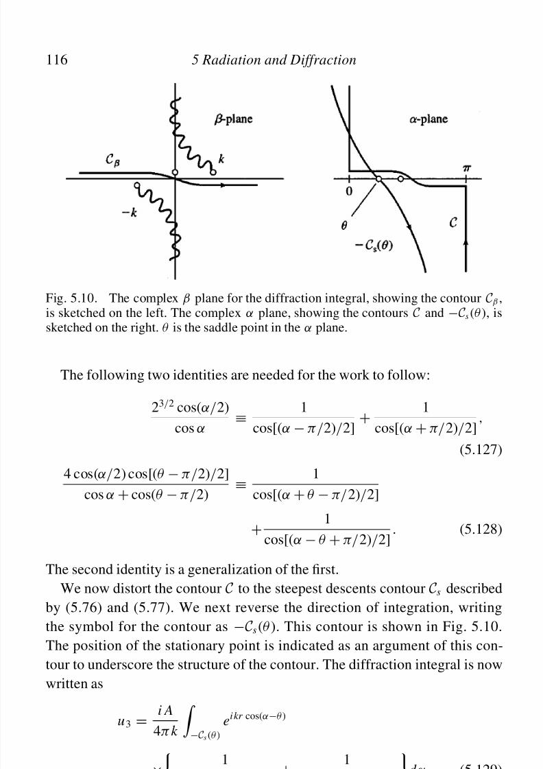
8/4/2019 Linear Elastic Waves (Cambridge Texts in Applied Mathematics) (John G. Harris) 0521643686
http://slidepdf.com/reader/full/linear-elastic-waves-cambridge-texts-in-applied-mathematics-john-g-harris 134/180
116 5 Radiation and Diffraction
Fig. 5.10. The complex β plane for the diffraction integral, showing the contour Cβ ,is sketched on the left. The complex α plane, showing the contours C and − Cs (θ ), issketched on the right. θ is the saddle point in the α plane.
The following two identities are needed for the work to follow:
23/ 2 cos( α/ 2)cos α
≡1
cos[( α − π/ 2) / 2]+
1cos[( α + π/ 2)/ 2]
,
(5.127)
4 cos( α/ 2) cos[( θ − π/ 2) / 2]cos α + cos( θ − π/ 2)
≡1
cos[( α + θ − π/ 2)/ 2]
+1
cos[( α − θ + π/ 2) / 2]. (5.128)
The second identity is a generalization of the rst.We now distort the contour C to the steepest descents contour Cs described
by (5.76) and (5.77). We next reverse the direction of integration, writingthe symbol for the contour as − Cs (θ ). This contour is shown in Fig. 5.10.The position of the stationary point is indicated as an argument of this con-tour to underscore the structure of the contour. The diffraction integral is nowwritten as
u 3 =i A
4π k − Cs (θ )e ikr cos( α − θ )
×1
cos[( α − π/ 2) / 2]+
1cos[( α + π/ 2) / 2]
d α, (5.129)
where (5.127) has been used.Setting aside the i A/ (4π k ), we consider the rst of the two integrals, which
we label I . We note that the calculation of the second is not different from that

8/4/2019 Linear Elastic Waves (Cambridge Texts in Applied Mathematics) (John G. Harris) 0521643686
http://slidepdf.com/reader/full/linear-elastic-waves-cambridge-texts-in-applied-mathematics-john-g-harris 135/180
Appendix: The Fresnel Integral 117
of the rst. We next change variables, giving
I =
1
2 − C s (0) ei kr cos α
×1
cos[( α + θ − π/ 2) / 2]+
1cos[( α − θ + π/ 2) / 2]
d α. (5.130)
Using (5.128), we can collapse this integral into the more symmetric form
I = 2
− C s (0)
cos( α/ 2) cos[( θ − π/ 2) / 2]
cos α + cos( θ − π/ 2)e ikr cos α d α. (5.131)
We now introduce yet another change of variables with the relation τ =21/ 2e i π/ 4 sin( α/ 2) (recall Problem 5.3 ). Thus the integral I becomes
I = − 2e i π/ 4e ikr η ∞
−∞
e− kr τ 2
τ 2 − i η2 d τ, (5.132)
where η = 21/ 2 cos[( θ − π/ 2) / 2].A third identity, namely
∞
kr e i η2ζ
∞
−∞e− ζ τ 2 d τ d ζ ≡ π 1/ 2
∞
kr ζ − 1/ 2e i η2ζ d ζ, (5.133)
is needed. Using this (interchange the order of integration on the left-hand side),we nd that
η ∞
−∞e
− kr τ 2
τ 2 − i η2 d τ = 2π1/ 2
η| η |
e− ikr η2
∞
| η | (kr )1/ 2e i µ 2 d µ
=2π 1/ 2η
| η |e− ikr η2
F | η | (kr )1/ 2 , (5.134)
where the Fresnel function F ( z), repeating the denition (5.103), is
F ( z) :=
∞
ze i ξ 2
d ξ. (5.135)
We now return to (5.129). Note that this integral contains both a pole contri-bution and a part composed of Fresnel integrals. Let u 3np represent the particledisplacement that does not include the pole contribution and u 3 p the pole con-tribution itself. Now u 3np is given by
u 3np =e− i π/ 4 A
π (1/ 2) k e− ikr cos( θ − π/ 2) F (2kr )1/ 2 cos
θ − π/ 2
2
± e− ikr cos( θ+ π/ 2) F ± (2kr )1/ 2 cosθ + π/ 2
2, (5.136)

8/4/2019 Linear Elastic Waves (Cambridge Texts in Applied Mathematics) (John G. Harris) 0521643686
http://slidepdf.com/reader/full/linear-elastic-waves-cambridge-texts-in-applied-mathematics-john-g-harris 136/180
118 5 Radiation and Diffraction
where the plus sign is used for θ ∈ (0 , π/ 2) and the minus sign for θ ∈ (π/ 2, π ).Here u 3 p is given by
u 3 p = − ( A/ k )e− ikr cos( θ − π/ 2) H (π/ 2 − θ ). (5.137)
Recalling (5.105),
F ( z) + F (− z) = π 1/ 2e i π/ 4 , (5.138)
we use it to combine (5.137) with the second term of (5.136) to give (5.104).
Problem 5.7 Asymptotic Approximations to the Fresnel Integral
Consider the Fresnel integral (5.135) for z = x, where x is real.
Problem 1. Find the rst term of an asymptotic expansion of the Fresnelintegral for both positive and negative x .
(a) Assume x > 0 and consider the integral
G ( x) = e− i x 2 ∞
xe i ζ 2
d ζ. (5.139)
Show that
G ( x) ∼i
2 x+ O ( x− 3), x → ∞ . (5.140)
One way to do this is to deform the contour to one such that Watson’s lemmacan be used.
(b) Assume x < 0. The approach of part (a) must be modied. Why? Write theintegral in (5.139) as one from x to −∞ and one from −∞ to ∞ . Do not
use (5.138). Hence show that
G ( x) ∼ π 1/ 2e i π/ 4e− i x 2+
i2 x
+ O ( x− 3), x → −∞ . (5.141)
That the two approximations differ for x that is positive or negative is anexample of the Stokes’ phenomena .
Problem 2. Find the rst term of an asymptotic expansion of the Fresnelintegral for | x| 1. Write the integral as the difference between one from zero

8/4/2019 Linear Elastic Waves (Cambridge Texts in Applied Mathematics) (John G. Harris) 0521643686
http://slidepdf.com/reader/full/linear-elastic-waves-cambridge-texts-in-applied-mathematics-john-g-harris 137/180
References 119
to ∞ and one from zero to x . Expand the integrand of the second integral in aTaylor expansion. Hence show that
F ( x) ∼ π 1/ 2e i π/ 4 / 2 − x + O ( x3), x → 0. (5.142)
References
Ablowitz, M.J. and Fokas, A.S. 1997. Complex Variables , pp. 411–513. New York:Cambridge.
Achenbach, J.D., Gautesen, A.K., and McMaken, H. 1982. Ray Methods for Waves in Elastic Solids . Boston: Pitman.
Babi c, V.M. and Buldyrev, V.S. 1991. Short-Wavelength Diffraction Theory . Berlin:Springer.
Born, M. and Wolf, E. 1986. Principles of Optics , 6th (corrected) ed., pp. 565–578.Oxford: Pergamon.
Cagniard, L. 1962. Reection and Refraction of Progressive Seismic Waves . Translatedand revised by E.A. Flinn and C.H. Dix. New York: McGraw-Hill.
Carrier, G.F., Krook, M., and Pearson, C.E. 1983. Functions of a Complex Variable ,pp. 249–283. Ithaca, NY: Hod Books.
Copson, E.T. 1935. An Introduction to the Theory of Functions of a Complex Variable ,pp. 121–125. Oxford: Clarendon Press.
Copson, E.T. 1971. Asymptotic Expansions , pp. 13–14 and 48–62. Cambridge:University Press.
Courant, R. and John, F. 1989. Introduction to Calculus and Analysis , Vol. II,pp. 345–350. New York: Springer
deHoop, A.T. 1960. A modication of Cagniard’s method for solving the seismic pulseproblem. Appl. Sc. Res. , B 8 : 349–356.
Doetsch, G. 1974. Introduction to the Theory and Application of the Laplace
Transform , pp. 218–230. New York: Springer.Ewing, W.M., Jardetzky, W.S., and Press, F. 1957. Elastic Waves in Layered Media .
New York: McGraw-Hill.Felsen, L.B. and Marcuvitz, N. 1994. Radiation and Scattering of Waves , pp. 370–441.
New York: IEEE and Oxford University Presses.Gautesen, A.K. 1979. On matched asymptotic expansions for two dimensional
elastodynamic diffraction by cracks. Wave Motion 1 : 127–140.Harris, J.G. 1980a. Diffraction by a crack of a cylindrical longitudinal pulse. Z. Angew.
Math. Phys. 31 : 367–383. Errata, Z. Angew. Math. Phys. 34 .
Harris, J.G. 1980b. Uniform approximations to pulses diffracted by a crack. Z. Angew. Math. Phys. 31 : 771–775.Harris, J.G. 1987. Edge diffraction of a compressional beam. J. Acoust. Soc. Am. 82 :
635–646.Harris, J.G. and Pott, J. 1985. Further studies of scattering of a Gaussian beam from a
uid-solid interface. J. Acoust. Soc. Am. 78 : 1072–1080.Hinch, E.J. 1991. Perturbation Methods , pp. 52–101. Cambridge: University Press.Holmes, M.H. 1995. Introduction to Perturbation Methods , pp. 47–104. New York:
Springer.
Jones, D.S. 1952. A simplifying technique in the solution of a class of diffractionproblems. Quart. J. Math. 3 : 189–196.Jull, E.V. 1981. Aperture Antennas and Diffraction Theory . London: Peter Peregrinus.

8/4/2019 Linear Elastic Waves (Cambridge Texts in Applied Mathematics) (John G. Harris) 0521643686
http://slidepdf.com/reader/full/linear-elastic-waves-cambridge-texts-in-applied-mathematics-john-g-harris 138/180
120 5 Radiation and Diffraction
Knopoff, L. and Gilbert, F. 1959. First motion methods in theoretical seismology. J. Acoust. Soc. Am. 31 : 1161–1168.
Noble, B. 1988. Methods Based on the Wiener-Hopf Technique , pp. 11–27 and 48–97.
New York: Chelsea.Titchmarsh, E.C. 1939. The Theory of Functions , 2nd ed., pp. 85–86 and 99–101.
Oxford: Clarendon Press.Titchmarsh, E.C. 1948. Introduction to the Theory of Fourier Integrals , 2nd ed.
Oxford: Clarendon Press.van der Pol, B. and Bremmer, H. 1950. Operational Calculus , pp. 122–132 and
elsewhere. Cambridge: University Press.Wong, R. 1989. Asymptotic Approximations of Integrals , pp. 20–31 and elsewhere.
Boston: Academic.
Zauderer, E. 1983. Partial Differential Equations of Applied Mathematics ,pp. 653–658 and 403–405. New York: Wiley-Interscience.

8/4/2019 Linear Elastic Waves (Cambridge Texts in Applied Mathematics) (John G. Harris) 0521643686
http://slidepdf.com/reader/full/linear-elastic-waves-cambridge-texts-in-applied-mathematics-john-g-harris 139/180
6
Guided Waves and Dispersion
Synopsis
Chapter 6 discusses guided waves and the dispersion they experience. Only theantiplane shear problem is treated. The guided waves are constructed by usingpartial waves and their dispersion calculated by using the transverse resonance
principle. Both harmonic and transient excitations of a closed waveguide arestudied by using an expansion of modes. The harmonic excitation of an openwaveguide by a line source is also studied, though in this case by using bothray and mode representations. As a last example, we examine propagation in aclosed waveguide with a slowly varying thickness, using an asymptotic expan-sion that combines features of both rays and modes. We close by examininghow information and energy propagate at the group velocity.
6.1 Harmonic Waves in a Closed Waveguide
We consider a layer of innite extent in the x1 direction and of nite thick-ness in the x2 direction. Within the layer, the coordinate x2 ∈ (− h , h ) and theplane x2 = 0 is a plane of reection symmetry. This structure is a waveguide orguide because the waves are forced to propagate in the x1 direction and theguide is closed because waves are completely trapped within the structure.We are interested in learning what kinds of antiplane waves propagate in theguide without, at present, seeking to know how they are excited. Accordingly,we seek possible solutions to the following antiplane problem. In the layer, u 3
must satisfy (2.20), which, rewritten here, is
∂a ∂a u 3 + k 2u 3 = 0, (6.1)
and at the surfacesµ∂ 2u 3( x1 , ± h ) = 0. (6.2)
121

8/4/2019 Linear Elastic Waves (Cambridge Texts in Applied Mathematics) (John G. Harris) 0521643686
http://slidepdf.com/reader/full/linear-elastic-waves-cambridge-texts-in-applied-mathematics-john-g-harris 140/180
122 6 Guided Waves and Dispersion
As in previous chapters the subscript T has been dropped. Problem 6.1 indicateshow solutions to this problem can be found by reducing it to an eigenvalue
problem in the transverse coordinate. When this is done we nd that the possiblewaveelds are described by
u 3m = Amcossin
(γ m x2)e iβ m x1 , m = 0, 1, 2, . . . , (6.3)
where u 3m is the m th (waveguide) mode for this guide. Cosine is used for meven and sine for m odd. This wave stands in the x2 direction, but it propagatesin the x1 direction. Here β m is the lateral wavenumber for the m th mode. Thetransverse wavenumbers for this mode are ± γ m . β m = ω/ cm , where cm is thephase velocity of the mode. β m is given by
β m = [k 2 − (mπ )2 / (2h )2]1/ 2 , (6.4)
where (β m ) ≥ 0 or (β m ) ≥ 0 for x1 > 0. In this particular case β m is either
real or imaginary, but not complex. For β m that is real, the wavenumber andphase velocity in the propagation direction depend on ω (through k = ω/ c).Thus (6.4) is a dispersion relation and is similar to that found previously forpropagation in periodic structures (there we used κ to represent the effectivewavenumber). The square root is dened so that, for imaginary values, the modedecays in its direction of propagation ( x1 > 0).
Introducing the term 1 e iβ x1 will reduce a linear partial differential equation,
or system of such equations, in ( x1 , x2) to an eigenvalue problem in x2 for β ,though that problem may not be easy to solve, or its solution may not be partic-ularly informative. However, by examining the solution, (6.3), we can learn toreconstruct it in a way that uses only the kinematical features of reection andtransmission of a plane wave at a boundary. Thereafter this method of solutioncan be used to solve other guided wave problems without directly consideringthe underlying eigenvalue problem.
Problem 6.1 An Eigenvalue Problem: A Closed Waveguide
Equation (6.1), with boundary condition (6.2), can be reduced to an ordinarydifferential equation in x2 by seeking solutions of the form
u 3 = f ( x2)e iβ x1 . (6.5)
1 This is equivalent to taking the spatial Fourier transform, transform variable β ,inthe x1 direction.

8/4/2019 Linear Elastic Waves (Cambridge Texts in Applied Mathematics) (John G. Harris) 0521643686
http://slidepdf.com/reader/full/linear-elastic-waves-cambridge-texts-in-applied-mathematics-john-g-harris 141/180
6.1 Harmonic Waves in a Closed Waveguide 123
Show that the differential equation in x2 leads to an eigenvalue problem for β 2 .Usually the β is linked with γ , where
γ = (k 2 − β 2)1/ 2 , (6.6)
and γ 2 or − γ 2 is considered the eigenvalue. In this book β 2 is considered theeigenvalue. Show that solutions symmetric with respect to the reection planeare
f 2n ( x2) = A2n cos γ 2n x2 , γ 2n = nπ/ h , (6.7)
and that those antisymmetric to this plane are
f 2n + 1( x2) = A2n+ 1 sin γ 2n+ 1 x2 , γ 2n+ 1 = (2n + 1)π/ (2h ), (6.8)
where n = 0, 1, 2, . . . . The Am are constants.
6.1.1 Partial Waves and the Transverse Resonance Principle
The central feature of a waveguide is that the waves phase match in the propa-gation direction and stand in the transverse direction. Equivalently stated, as thewaves reect back and forth within the guide, they must interfere constructivelyto reconstruct themselves and form a sustained waveeld. There are two sets of plane waves in a guide, as indicated in Fig. 6.1 – one propagating downward
and one upward. The members of each set are referred to as partial waves, justas were the individual plane waves in each cell of the periodic structure exam-ined in Section 1.4. Those that propagate downward are indicated by the solidlines and those that propagate upward by the dashed ones. The downward and
Fig. 6.1. The dashed lines indicate the upward propagating set of plane waves, whilethe solid lines indicate the downward propagating set. These rays are shown in theslowness diagram to the right. Note that phase matching must occur in the x1 direction.

8/4/2019 Linear Elastic Waves (Cambridge Texts in Applied Mathematics) (John G. Harris) 0521643686
http://slidepdf.com/reader/full/linear-elastic-waves-cambridge-texts-in-applied-mathematics-john-g-harris 142/180
124 6 Guided Waves and Dispersion
upward propagating sets are
u 3 = Ae i (β x1 − γ x2 ) , (6.9)
u 3 = Be i (β x1 + γ x2 ) , (6.10)
respectively. The term γ is given by (6.6). We have, at this stage, assumedonly that (γ ) ≥ 0. From our previous work, given in Section 3.2, we can,by a slight modication of that calculation, show that the reection coefcientat x2 = ± h is one. Each upward propagating wave must be reected into adownward propagating one and vice versa. Therefore, at the upper and lowerboundaries,
Ae− i γ h
Bei γ h= 1, (6.11)
Be− i γ h
Ae i γ h= 1, (6.12)
respectively. The terms A and B are constants. For these two equations to holdsimultaneously, the following must be true:
γ h = mπ/ 2, (6.13)
and
A = B for m = 2n , n = 0, 1, 2, . . . (6.14)
or
A = − B for m = 2n + 1, n = 0, 1, 2, . . . . (6.15)
Therefore
u 3m = Amcossin
(γ m x2)e iβ m x1 , m = 0, 1, 2, . . . , (6.16)
where β m is given by (6.4), γ m = mπ/ 2h , and Am is 2 A or 2 i A. This method of nding the dispersion relation, (6.4), wherein partial waves are made to standor resonate in the transverse direction, is referred to as the transverse resonance principle .
6.1.2 Dispersion Relation: A Closed Waveguide
The most intriguing feature of guided waves is that the lateral wavenumber β m
is a function of ω , or, alternatively ω is a function of β m . The dispersion relation

8/4/2019 Linear Elastic Waves (Cambridge Texts in Applied Mathematics) (John G. Harris) 0521643686
http://slidepdf.com/reader/full/linear-elastic-waves-cambridge-texts-in-applied-mathematics-john-g-harris 143/180
6.1 Harmonic Waves in a Closed Waveguide 125
Fig. 6.2. A sketch of the dispersion relation for antiplane shear modes in a closedwaveguide. The normalized angular frequency is plotted as a function of the normalizedlateral wavenumber.
can be written as
2hβ m = [(2hω/ c)2 − (mπ )2]1/ 2 . (6.17)
A sketch of this relation is shown in Fig. 6.2. While the β m may be thought of asa function of ω , when the frequency is a free variable, it is usual to consider ω asa function of β m . For the m th mode, there is no propagation for (2 hω/ c) ≤ mπand the frequency ωm = mπ c/ 2h is called the cut-off frequency. The phasevelocity cm for the m th mode is
cm = ω/β m . (6.18)
The velocity of real interest, however, is the group velocity Cm . Unlike cm , Cm
for the m th mode is given by the slope of the m th branch of the dispersionrelation, namely
Cm = d ω/ d β m . (6.19)
The group velocity is both the velocity of energy propagation and the velocitywith which information propagates. Here we demonstrate the rst assertionand leave to Section 6.6 the demonstration of the second. The time average of awaveeld quantity Gm (β m x1 − ω t , x2)forthe m th waveguide mode is dened as
Gm = 1T t + T
t h
− hGm (β m x1 − ωτ, x2)dx2d τ. (6.20)

8/4/2019 Linear Elastic Waves (Cambridge Texts in Applied Mathematics) (John G. Harris) 0521643686
http://slidepdf.com/reader/full/linear-elastic-waves-cambridge-texts-in-applied-mathematics-john-g-harris 144/180
126 6 Guided Waves and Dispersion
The average Gm does not depend upon x1 or t because at a given x1 , theargument β m x1 − ωτ is simply a translation of the argument ωτ , a fact notedpreviously when deriving (2.18).
The instantaneous energy density E m ( x1 , x2 , t ) in the m th mode is
E m = 12 ρ ∂ t u 3m ∂t u 3m + 1
2 µ ∂ a u 3m ∂a u 3m , (6.21)
and, using (6.20) with (2.18), we nd that its average is
E m = 12 ρ c2
m hβ 2m Am A∗m . (6.22)
For propagation β m is real. The instantaneous ux of energy densityF m ( x1 , x2 , t ) in the m th mode is
F m = − µ∂ 1u 3m ∂t u 3m , (6.23)
and the average ux is
F m = 12 µ cm hβ 2
m Am A∗m . (6.24)
The velocity of energy propagation along the axis of the waveguide for the m thmode is, therefore, the ratio F m / E m . Direct calculation shows that
F m / E m = c2 / cm = Cm . (6.25)
The average (6.20) can also be used to demonstrate the equipartition of energy. Using this principle whencalculating the average energy density, insteadof proceeding directly as we just did, usually reduces the amount of calculationneeded, though care is required because not all equations describing waveeldsexhibit equipartition. The Lagrangian density L for antiplane shear motion isgiven by
L = 12 ρ (∂t u 3)2 − 1
2 µ [(∂1u 3)2 + (∂2u 3)2]. (6.26)
Using (6.20) we readily nd that L = 0, for the m th mode. It follows thenthat K = U , where the kinetic and internal energy densities, K and U , wererst dened by (1.25). Clearly, the converse is also true.
Dispersion need not arise from a geometrical constraint, as it does witha waveguide, but can arise from the structure of the equation itself, as thefollowing problem demonstrates.

8/4/2019 Linear Elastic Waves (Cambridge Texts in Applied Mathematics) (John G. Harris) 0521643686
http://slidepdf.com/reader/full/linear-elastic-waves-cambridge-texts-in-applied-mathematics-john-g-harris 145/180
6.1 Harmonic Waves in a Closed Waveguide 127
Problem 6.2 Dispersion 1
Problem 1. Consider the following two differential equations, the Klein–Gordon equation,
∂ 2t ϕ − a 2∂ 2
xϕ + b2ϕ = 0, (6.27)
and the equation for exural motion in a rod,
∂ 2t ϕ + a 2∂ 4
xϕ = 0. (6.28)
The terms a and b are constants. In both cases nd a dispersion relation in theform ω = ω(k ) by seeking a wave solution of the form
ϕ = Aei (kx− ω t ) , (6.29)
where A is a constant. Assume that the wave propagates to the right. Calculatethe phase and group velocities c and C , where c = ω/ k and C = d ω/ dk .
Demonstrate that the group velocity is the velocity of time-averaged energytransport. To do so you will need to know both the instantaneous energy densityand instantaneous ux, so that you can calculate their average values. One wayto nd these is to construct conservation laws directly from (6.27) and (6.28).Such laws have the form
∂t + ∂ x = − . (6.30)
The rst box is the instantaneous energy density, the second the instantaneousux, and the third, on the right-hand side, a dissipative term. For the equa-tions being studied here, the right-hand side is zero. To nd a conservationlaw, multiply each of (6.27) and (6.28) by ∂t ϕ and congure the result to co-incide with (6.30). Thus, show that the instantaneous energy density for theKlein–Gordon equation is
E = (∂t ϕ)2 / 2 + a 2(∂ xϕ)2 / 2 + b2ϕ2 / 2 (6.31)
and the instantaneous ux is
F = − a 2(∂t ϕ)(∂ xϕ). (6.32)
Also, show that the instantaneous energy density for the equation for exuralmotion is
E = (∂t ϕ)2 / 2 + a 2 ∂ 2 xϕ
22 (6.33)

8/4/2019 Linear Elastic Waves (Cambridge Texts in Applied Mathematics) (John G. Harris) 0521643686
http://slidepdf.com/reader/full/linear-elastic-waves-cambridge-texts-in-applied-mathematics-john-g-harris 146/180
128 6 Guided Waves and Dispersion
and the instantaneous ux is
F = a 2(∂t ϕ) ∂ 3 xϕ − a 2(∂t ∂ xϕ) ∂ 2
xϕ . (6.34)
Using (2.18), complete the demonstration.
Problem 2. The equation describing acoustic waves in a wind having speedU (< c , where c is the speed of sound) in the x1 direction is given by
(∂t + U ∂1)2ϕ = c2
∇2ϕ, (6.35)
where ( x , t ) is a xed coordinate system. Using a solution of the form
ϕ = Aei ( k · x − ω t ) , (6.36)
nd the dispersion relation. The vector k is needed because the propagationenvironment is anisotropic.
6.2 Harmonic Waves in an Open Waveguide
We continue to consider an antiplane problem having the governing equation,(6.1). We now consider a layer on a half-space. Figure 6.3 indicates the geome-try. Note that the positive x2 direction points into the interior. The interior of the
Fig. 6.3. A slow-on-fast structure can support trapped waves in the layer. Drawing
slowness diagrams for the layer and half-space indicates the condition for waves to betrapped in the layer, namely that the vertical dashed line in the diagram to the right notintersect the lower slowness circle.

8/4/2019 Linear Elastic Waves (Cambridge Texts in Applied Mathematics) (John G. Harris) 0521643686
http://slidepdf.com/reader/full/linear-elastic-waves-cambridge-texts-in-applied-mathematics-john-g-harris 147/180
6.2 Harmonic Waves in an Open Waveguide 129
layer occupies x2 ∈ (− h , 0) and its wavespeed is c (k = ω/ c). The equation of motion in the layer is (6.1). The interior of the half-space occupies x2 ∈ (0 , ∞ ).
The equation of motion in the half-space is also given by (6.1) with a differentwavenumber. The equation, rewriting it once again, is
∂α ∂α u 3 + k 2u 3 = 0, (6.37)
where k = ω/ c and c is the wavespeed in the half-space. At x2 = − h ,
µ∂ 2u 3( x1 , − h ) = 0, (6.38)
and at x2 = 0,
u 3( x10− ) = u 3( x10+ ), µ∂ 2u 3( x1 , 0− ) = µ∂ 2u 3( x1 , 0+ ), (6.39)
where µ and µ are the elastic constants for the layer and half-space, respectively.The layer is called an open waveguide because there is now the possibility
that waves may not remain trapped, but may radiate into the half-space. How-ever, waves will remain trapped provided the wavespeed in the layer is lessthan that in the half-space. This conguration is sometimes referred to as aslow-on-fast guiding structure. To understand why waves are trapped, considerthe slowness diagrams sketched in Fig. 6.3. The wavespeed in the layer is cand that in the underlying half-space c, so that the corresponding slownessesare s and s , respectively. A slow-on-fast structure is one for which s > s . If thewaves are to phase match at x2 = 0, s1 must be the same in both the layer andhalf-space. If the waves are to remain trapped in the layer, unable to radiateaway, s 2 must be imaginary, with the sign of s 2 selected so that decay takesplace with depth. Therefore, the waves in the layer able to phase match to wavesdecaying into the half-space are those for which s1 = s1 > s . When s1 ≤ s < s ,waves launched in the layer phase match to waves in the half-space for whichs 2 is real and are therefore not trapped. The slow-on-fast structure is analyzednext by using partial waves and the transverse resonance principle. In Problem6.3 the problem is reduced to solving an eigenvalue problem in the x2 direction.A fast-on-slow structure ( s < s ) does not guide waves so that, except inProblem 6.4 , we do not consider it.
6.2.1 Partial Wave Analysis
In the layer, the upward and downward propagating sets of waves are
u 3 = Bei (β x1 − γ x2 )
, (6.40)u 3 = Aei (β x1 + γ x2 ) . (6.41)

8/4/2019 Linear Elastic Waves (Cambridge Texts in Applied Mathematics) (John G. Harris) 0521643686
http://slidepdf.com/reader/full/linear-elastic-waves-cambridge-texts-in-applied-mathematics-john-g-harris 148/180
130 6 Guided Waves and Dispersion
In the half-space the set of waves is
u 3 = ¯ Ae i (β x1 + γ x2 ) . (6.42)
The waves in the half-space decay or propagate downward. This statement isconsistent with the principle of limiting absorption, given in Section 4.4. Tosatisfy the equations of motion,
γ = (k 2 − β 2)1/ 2 , γ = (k 2 − β 2)1/ 2 , (6.43)
where (γ ) ≥ 0 and ( γ ) ≥ 0. We discuss the branches of these radicals morecarefully in Section 6.4. The reection and transmission coefcients at x2 = 0are, respectively,
R(γ ) = (µγ − µ γ )/ (µγ + µ γ ), (6.44)
T (γ ) = (2µγ )/ (µγ + µ γ ). (6.45)
The R(γ ) and T (γ ) are gotten from (3.21) and (3.22) by noting that β =
k sin θ0 = k sin θ2 , γ = k cos θ0 , and γ = k cos θ2 . Exactly as in the case of theclosed guide, at x2 = − h ,
Ae− i γ h / Bei γ h = 1, (6.46)
and at x2 = 0,
B/ A = (µγ − µ γ )/ (µγ + µ γ ). (6.47)
Moreover, in the case of the open guide, we also have
¯ A/ A = (2µγ )/ (µγ + µ γ ). (6.48)
These last two equations indicate that plane waves incident on the lower bound-ary must, in addition to being reected, be transmitted into those that decay orpropagate away from the boundary. From (6.46) and (6.47) we nd that fornontrivial solutions,
e− 2i γ h = (µγ − µ γ )/ (µγ + µ γ ). (6.49)
The case of interest is s < s1 ≤ s , where β = ωs1 , so that γ = i α , where α ≥ 0.In this case (6.49) reduces to
tan γ h = µ α/µγ. (6.50)
Recalling (6.43), we see that (6.49) or (6.50) is the dispersion relation for thestructure. It gives ω = ω (β ) or β = β (ω), albeit indirectly. The antiplane waves

8/4/2019 Linear Elastic Waves (Cambridge Texts in Applied Mathematics) (John G. Harris) 0521643686
http://slidepdf.com/reader/full/linear-elastic-waves-cambridge-texts-in-applied-mathematics-john-g-harris 149/180
6.2 Harmonic Waves in an Open Waveguide 131
guided by the layer are called Love waves . Knowing the dispersion relation,we can nd B and ¯ A in terms of A, and thus construct the waveelds in the
layer and half-space. Note that the absence of a plane of reection symmetrymeans that the modes do not divide into symmetric and antisymmetric ones.
Problem 6.3 A Second Eigenvalue Problem: An Open Waveguide
Note that (6.29) and (6.30), with boundary conditions (6.31) and (6.32), canbe reduced to a singular eigenvalue problem (Friedman, 1956) in x2 by lookingfor solutions of the form
u 3 = f ( x2)e iβ x1 , x2 ∈ (− h , 0) , (6.51)
u 3 = g( x2)e iβ x1 , x2 ∈ (0 , ∞ ). (6.52)
Note that the form of the function in x1 has been chosen to give a wave prop-agating in the positive x1 direction and ensure phase matching at x2 = 0. Usethe condition that g( x2) → 0 as x2 → ∞ . Show that solutions to the differentialequation in x2 and its boundary conditions can be expressed as
f ( x2) = C cos[ γ ( x2 + h )], g( x2) = De − α x2 , (6.53)
where γ = i α , α ≥ 0. The transverse wavenumbers γ and γ are given by (6.36).Find the constant D in terms of C . Can you recover the dispersion relationship,(6.50)?
The problem just discussed is called a singular eigenvalue problem because ithas a continuous spectrum as well as a discrete one. The preceding analysis givesthe discrete eigenvalues and eigenfunctions, but gives one little informationabout the continuous spectrum, unless the reader is quite perceptive. Friedman(1956), mentioned previously, will help the reader understand the underlyingmathematics of singular eigenvalue problems; Tolstoy and Clay (1987) willgive the reader a reasoned physical explanation for the continuous spectrum.
What condition stated previously in this problem must be modied to nd thecontinuous eigenvalues and eigenfunctions?
6.2.2 Dispersion Relation: An Open Waveguide
The transcendental equation, (6.50), in combination with (6.43), gives eitherω = ω (β ) or β = β (ω ). To examine this dispersion relation, we begin witha diagram such as that shown in Fig. 6.4, where three distinct regions are
identied. First we identify the boundaries between which β is real (assumingthat c < c). These boundaries are denoted by c and c, though the slopes are 1and c/ c.

8/4/2019 Linear Elastic Waves (Cambridge Texts in Applied Mathematics) (John G. Harris) 0521643686
http://slidepdf.com/reader/full/linear-elastic-waves-cambridge-texts-in-applied-mathematics-john-g-harris 150/180
132 6 Guided Waves and Dispersion
Fig. 6.4. A sketch of the dispersion relation for Love waves. The normalized angularfrequency is plotted as a function of the normalized lateral wavenumber. There are threeregions whose boundaries are formed by the two wavespeeds c < c.
In region 1, γ = ± i α and γ = i α , where α and α are real and positive. Itis readily seen that no solution for real β is possible and therefore no trappedwave propagates in the x1 direction. In region 3 both γ and γ are real. In thiscase (6.43) becomes
tan( γ h ) = − i µ γ/µγ. (6.54)
Again it is clear that there is no solution for β that is real, though there aresolutions for complex β . We shallbriey discuss this possibility in Section 6.4.3.The absence of roots for β real tells us that there are no trapped waves, exactlywhat we would expect for γ and γ both real.
Solutions for real β are possible in region 2, as can be seen from examining(6.50). Consider the following limits. First, let β h → ∞ within region 2. Write(6.50) as
tan β h [(k 2 /β 2) − 1]1/ 2 =µ [1 − (k 2 /β 2)]1/ 2
µ [(k 2 /β 2) − 1]1/ 2 . (6.55)
The argument of the tangent in (6.55) approaches a nite limit or zero becausethe right side remains positive, and approaches zero or +∞ . There is only onepossibility, namely k /β → 1. In other words, by allowing the layer to becomean innite number of wavelengths thick, its response is no longer inuencedby the presence of the half-space. Second, let β h move toward zero throughregion 2 and reason as before. For the lowest mode k /β → 1 as β h → 0 and

8/4/2019 Linear Elastic Waves (Cambridge Texts in Applied Mathematics) (John G. Harris) 0521643686
http://slidepdf.com/reader/full/linear-elastic-waves-cambridge-texts-in-applied-mathematics-john-g-harris 151/180
6.2 Harmonic Waves in an Open Waveguide 133
ωh → 0. However, for the higher modes k /β → 1, while β h and ωh remainnite. In this case, for some ω = ωn , α = 0 and
[(ωn h /β hc )2 − 1]1/ 2β h = nπ, (6.56)
where n is a positive integer. The frequency ωn is that at which the wavesmove from being trapped to radiating into the half-space. This frequency is alsocalled a cut-off frequency, though the term transition frequency might be moreappropriate. Unlike the case of a closed waveguide, the group velocity does not
vanish at this point. Keep in mind that we have, so far, restricted β to positivereal values and have not dened the branches of γ and γ carefully.The outcomes of the problem just described should be compared with those
of the reection problem that follows. The viewpoint there is rather different.In the reection problem the layer is viewed from the half-space, and we are nolonger as concerned as we were here with whether the structure is a slow-on-fastor fast-on-slow one.
Problem 6.4 Reection From a Layer
Referring to the geometry of Fig. 6.3, let the plane wave
u 30 = A0e i (β x1 − γ x2 ) (6.57)
be incident to the layer from the half-space. Make no assumption at present asto the relative magnitudes of c and c. If A1 is the unknown amplitude of thereected wave, calculate the reection coefcient of the layer, namely R(θ0) =
A1 / A0 . Show that R(θ0) = A− (θ0)/ A+ (θ0), where
A∓ = cos θ0 cos( kh cos θ ) ∓ iµ cµ c
cos θ sin( kh cos θ ), (6.58)
and
sin θ/ c = sin θ0 / c. (6.59)
The wavenumbers β = k sin θ0 and γ = k cos θ0 .The reader should contrast the two possible cases, fast-on-slow and slow-on-
fast. In particular, how might a trapped wave be excited by using a disturbanceincident from the half-space when the structure is slow on fast? Note that thisreection coefcient is frequency dependent.
8/4/2019 Linear Elastic Waves (Cambridge Texts in Applied Mathematics) (John G. Harris) 0521643686
http://slidepdf.com/reader/full/linear-elastic-waves-cambridge-texts-in-applied-mathematics-john-g-harris 152/180
134 6 Guided Waves and Dispersion
6.3 Excitation of a Closed Waveguide
6.3.1 Harmonic Excitation
We start by considering a closed waveguide that is harmonically excited byapplying an antiplane traction at one end, while the other extends to innity.One common way to solve such problems is to expand the waveeld in the guidein terms of its modes. To do so requires that a mathematical framework be inplace. As a minimum we need a means of calculating the coefcients of theexpansion – an orthogonality relation – and some assurance that the expansionis complete. While these questions have still not been satisfactorily answeredfor inplane elastic waves in a guide with an end (Miklowitz, 1978; Folgueraand Harris, 1999), the antiplane modes are simply the terms of a Fourier series,so that in this case these questions are settled.
Problem 6.5 A Waveguide Mode Expansion
In part, (6.1) and (6.2) specify the problem. The geometry of the problem isnow described by a layer similar to that shown in Fig. 6.1, but starting at x1 = 0and extending through positive values of x1 to innity. At x1 = 0 the waveguideis excited with a traction T ( x2) symmetric in x2 so that
µ∂ 1u 3 = − T ( x2), T ( x2) = T (− x2). (6.60)
What condition should be imposed upon the forced disturbance as x1 → ∞ ?
Noting the symmetry of the excitation, how might the forced waveeld beexpanded? Show that a representation of the solution is
u 3( x1 , x2) = N − 1
n= 0
(− An )iβ n
cosnπh
x2 e iβ n x1 +∞
n= N
An
α ncos
nπn
x2 e− α n x1 ,
(6.61)
where N is the smallest n for which the inequality
nπ/ h < ω/ c (6.62)
is reversed. The frequency of excitation is ω , β n is given by (6.4), and, forn ≥ N , β n = i α n . Using the orthogonality of the modes (eigenfunctions), writedown explicit expressions for the coefcients An .
Note that the modes in the rst sum of (6.61) propagate, while those in thesecond are evanescent. Far from the source, only those that propagate make asignicant contribution.

8/4/2019 Linear Elastic Waves (Cambridge Texts in Applied Mathematics) (John G. Harris) 0521643686
http://slidepdf.com/reader/full/linear-elastic-waves-cambridge-texts-in-applied-mathematics-john-g-harris 153/180
6.3 Excitation of a Closed Waveguide 135
6.3.2 Transient Excitation
We next consider a transient excitation. In Problem 6.5 , we replace (6.60) with
µ∂ 1u 3 = − T ( x2)δ(t ). (6.63)
Moreover, we assume that the waveguide is quiescent until the excitation isapplied. That is,
u 3 = ∂t u 3 = 0, t < 0. (6.64)
Using (1.36), we synthesize the transient response as
u 3( x1 , x2 , t ) =∞
n= 0
(− An )π
cosnπh
x2 ∞
0
e i t (β n x1 / t − ω )
iβ nd ω. (6.65)
Using the principle of limiting absorption, replace ω with ω + i , where > 0.The n = 0 term is easily inverted, giving
∞
0
e i (ω+ i )( x1 / c− t )
i (ω + i )/ cd ω = − π c H (t − x1 / c). (6.66)
The n > 0 terms are less straightforward. The integral to be evaluated is
∞
0
e i x1 (β n − ω t / x1 )
iβ nd ω. (6.67)
The left half of Fig. 6.5 shows the complex ω plane and the branch cuts forn > 0. Following the arguments in Section 3.4.4, we have cut the plane so that
(β n ) ≥ 0 for all ω . Using the principle of limiting absorption for ω > 0, wend the branch point is at c n π/ h − i . By symmetry, for ω < 0, the branchpoint is at − cn π/ h + i . The integration contour in the ω plane must pass abovethe branch point cn π/ h − i . Note that c n π/ h is a cut-off frequency so thatpropagation has ceased when ω < cn π/ h . Note, as well, that (β n ) > 0 in therst and third quadrants. Once the contour has been determined, the in (6.67)can be set to zero.
Integrals of the form of (6.67), even when they can be evaluated in closedform, give the clearest description of the waveeld at points far from the source.Accordingly, we approximate (6.67) by using the method of stationary phasedescribed in Section 5.3.3. We x t / x1 and let x1 be the large parameter. For a

8/4/2019 Linear Elastic Waves (Cambridge Texts in Applied Mathematics) (John G. Harris) 0521643686
http://slidepdf.com/reader/full/linear-elastic-waves-cambridge-texts-in-applied-mathematics-john-g-harris 154/180
136 6 Guided Waves and Dispersion
Fig. 6.5. The left-hand gure shows the complex ω plane. The contour extends fromω = 0 along the real axis. (β n ) ≥ 0 ∀ω, (β n ) > 0 in the upper right quadrant of theω plane. The right-hand gure shows the dispersion curve for the n th mode with thestationary point indicated by ( β ns , ω ns ).
given point in ( x1 , t ), the stationary point is given by
d β n / d ω = t / x1 . (6.68)
Solving this equation gives the stationary point ( β ns , ω ns ) as a function of ( x1 , t )(more precisely x1 / t ), namely
ωns
c= nπ/ h
[1 − ( x1/ ct )2]1/ 2 , x1 / ct < 1, (6.69)
and
β ns =nπh
x1 / ct [1 − ( x1 / ct )2]1/ 2 , x1 / ct < 1. (6.70)
No signal can travel faster than c (Problem 6.6 ). Therefore, x1 / ct < 1 for prop-agating waves and ( β ns , ω ns ) are real.
The integral, (6.67), is then approximated as
∞
0
e i x1 (β n − ω t / x1 )
iβ nd ω ∼
c (2π )1/ 2
(nπ/ h )(β ns x1)1/ 2e i x1 (β ns − ωns t / x1 )e− i π/ 4 ,
(6.71)
as x1 → ∞ , while t / x1 is held xed. After some simplication, the particle

8/4/2019 Linear Elastic Waves (Cambridge Texts in Applied Mathematics) (John G. Harris) 0521643686
http://slidepdf.com/reader/full/linear-elastic-waves-cambridge-texts-in-applied-mathematics-john-g-harris 155/180
6.3 Excitation of a Closed Waveguide 137
displacement of the n th mode is approximated as
u 3n ( x1 , x2 , t ) ∼ (− An )π
c cos nπh
x2 (2h / n) x1[(ct / x1)2 − 1]1/ 2
1/ 2
× cos (nπ/ h ) x1[(ct / x1)2 − 1)] 1/ 2 + π/ 4 , (6.72)
and the total particle displacement can be written as
u 3( x1 , x2 , t ) ∼ A0c H (t − x1 / c) +
∞
n= 1u 3n ( x1 , x2 , t ). (6.73)
Examining (6.72) shows that the n th mode is O( n − 1/ 2). The higher-order modestherefore make a weaker contribution than do the lower-order ones.
Note that the stationary phase approximation breaks down for x1 / t near c.Dai and Wong (1994) give a correction for this case. Further, note that as x1 / t sweeps through its values from zero to c, ωs takes on all its values from cn π/ h
to innity. In fact, for xed x1 , (6.68) provides a one-to-one mapping from thet plane to the ω plane.
At ( x1 , t ) the n th mode is approximated by an expression of the form
An ( x1 , x2 , t )e i (β ns x1 − ωns t ) . (6.74)
This is a group in the sense that it arises from a cluster or group of wavenum-
bers and frequencies in the neighborhood of ( β ns , ω ns ). Note that (6.68) canbe viewed as x1 / t = Cn (ωns ), where Cn is the group velocity d ω/ d β n . We havealready noted in (6.25) that Cn is the velocity of time-averaged energy trans-mission. Now we also note that it is the velocity with which the frequency ωns
propagates to the point ( x1 , t ). This is not the velocity with which the phaseθ ( x1 , t ) = (β ns x1 − ωns t ) propagates outward. Rather, a constant phase θ prop-agates at a rate cns = ωns /β ns .
Problem 6.6 No Signal Travels Faster than the Velocity c
Using the problem just discussed, show that no signal travels faster than c.Write each integral over ω as
π
∞
0
e− i ω (t − x1 / c) e i (β n x1 − ω x1 / c)
iβn
d ω (6.75)
and note that, in the upper right quadrant of Fig. 6.5, with the ω plane cut as

8/4/2019 Linear Elastic Waves (Cambridge Texts in Applied Mathematics) (John G. Harris) 0521643686
http://slidepdf.com/reader/full/linear-elastic-waves-cambridge-texts-in-applied-mathematics-john-g-harris 156/180
138 6 Guided Waves and Dispersion
indicated,
lim| ω |→∞
e i (β n x1− ω x1 / c)
iβ n= 0. (6.76)
Therefore, for t < x1 / c , show that the integration contour may be distorted fromone along the real ω axis to the one along the imaginary axis. Lastly, show thatthe integral can be written as
π ∞
0 i e p(t − x1 / c) e− (αn x1− px1 / c)
(− α n ) dp . (6.77)
This integral must be zero (why?), indicating that no signal is present for t < x1 / c .
While this result is the outcome of the analysis of a specic problem, it istrue generally. Moreover, it indicates that the group velocity does not exceedthe wavespeed of the medium, 2 a result that is also generally true.
For separable problems, such as the one discussed in Problem 6.5 , an expan-sion of the solution in the eigenfunctions of the transverse eigenvalue problemresults, after invoking the orthogonality of the eigenfunctions, in reducing thepartial differential equation to an ordinary one in x1 , involving each modeseparately. The domain of the transverse eigenvalue problem is nite and there-fore the eigenvalues are discrete. Expanding the source in these eigenfunctions
causes the equation in x1 to be forced by a coefcient of this expansion. This ismore or less what we did in solving Problem 6.5 , though the modal expansionalready contained the solution to the differential equation in x1 , so that that stepwas leaped over. In Problem 6.7 the reader is asked to solve much the sameproblem by using a continuous eigenfunction expansion in x1 ∈ (0 , ∞ ), thusreducing the partial differential equation to an ordinary one in x2 . Moreover,rather than use a Fourier synthesis to construct the transient solution, the reader
is asked to use a Laplace transform.
2 The dispersion is said to be anomalous when the group velocity exceeds the velocity of propa-gation of a harmonic plane wave in the medium (Sommerfeld, 1964a; Brillouin, 1960). In thiscase the group velocity is no longer a measure of the speed at which information or energypropagates. In such cases a specic signaling problem must be worked through, and veloc-ities that characterize the speed at which information is propagated and at which energy ispropagated must be dened as best one can. Moreover, the anomalous dispersion may only beapparent and not real. One must take care to distinguish between anomalous dispersion caused
by some approximate derivation of the equation being studied and that caused by the underly-ing physical situation. The presence of frequency-dependent attenuation confuses the issue evenfurther.

8/4/2019 Linear Elastic Waves (Cambridge Texts in Applied Mathematics) (John G. Harris) 0521643686
http://slidepdf.com/reader/full/linear-elastic-waves-cambridge-texts-in-applied-mathematics-john-g-harris 157/180
6.4 Harmonically Excited Waves in an Open Waveguide 139
Problem 6.7 A Continuous Eigenfunction Expansion
Continue to consider the problem just solved, with the excitation (6.63). Use
the cosine transform
∗u 3(ξ, x2 , t ) = ∞
0u 3( x1 , x2 , t ) cos( ξ x1)dx1 , (6.78)
followed by the Laplace transform
∗u 3(ξ, x2 , p) = ∞
0
∗u 3(ξ, x2 , t )e pt dt , (6.79)
to nd an ordinary differential equation in x2 . Find ∗u 3 and begin to invert thetransforms. It is perhaps easier to set ∗v3(ξ, x2 , p) = p∗u 3(ξ, x2 , p) where v3
is the particle velocity. Find
∗v3(ξ, x2 , t ) =1
2π i + i ∞
− i ∞
∗v3(ξ, x2 , p)e pt dp (6.80)
and then approximate
v3( x1 , x2 , t ) =2π
∞
0
∗v3(ξ, x2 , t ) cos( ξ, x1)d ξ (6.81)
for large x1 , with x1 / t held xed, using the method of stationary phase. Thisintegral can also be inverted exactly.
The reader may be surprised to nd that his or her expression for v3 containsboth forward and backward propagating waves. This is because we have chosento work with a cosine transform.Why would one not work with a sine transform?At what point has the reader imposed the condition that waves be outgoing fromthe source? Can the reader express (6.81) as a sum of waves propagating solelyin the positive x1 direction?
6.4 Harmonically Excited Waves in an Open Waveguide
We next return to the layered antiplane structure, sketched on the left in Fig. 6.3,to calculate the waveeld radiated by a harmonic line source placed at (0 , x20 ),where x20 < 0. Except for the absence of a source, the equations of motionand the boundary conditions are given by (6.38) and (6.39). This problemmay be solved by constructing the solution by using eigenfunction expansions.However, as we have done previously, we shall construct the radiated waveeldby superposing collections of partial waves. This method of construction will
show how ray representations and modal expansions are related to one another.Our discussion follows a very similar one in Brekhovskikh (1980).

8/4/2019 Linear Elastic Waves (Cambridge Texts in Applied Mathematics) (John G. Harris) 0521643686
http://slidepdf.com/reader/full/linear-elastic-waves-cambridge-texts-in-applied-mathematics-john-g-harris 158/180
140 6 Guided Waves and Dispersion
6.4.1 The Waveeld in the Layer
We begin by representing the waveeld radiated by a line source asa spectrum of
plane waves, using the result of Problem 4.1 . Equation (4.19), with α replacingξ , is here rewritten by expanding cos( θ − α ) to give
u i3 = −
i F 04π C
e ik ( x1 cos α +| x2 − x20 | sin α )d α. (6.82)
F 0 = A/ k , where A is a dimensionless constant. The expression (6.82) givesthe free space, particle displacement u i
3 excited by a line source at (0 , x20 ). The
contour C begins near π − i ∞ and ends near i ∞ . How then does each planewave in the integral, (6.82), behave in the layered environment?
Consider an arbitrary observation point ( x1 , x2) in the layer, where x1 > 0and x2 > x20 . Given that the x1 dependence must be of the form e ik cos α x1 , in boththe layer and half-space, to ensure phase matching, we ask what partial wavescan reach the point ( x1 , x2) and, when added together, satisfy the boundaryconditions. By sketching rays and wavefronts, as suggested in Fig. 6.6, we
nd that there are four distinct partial waves that reach ( x1 , x2) and that all thesubsequent partial waves can be constructed from these four by successivelyreecting them in the planes x2 = 0 and x2 = − h .
e ik [ x1 cos α + sin α ( x2 − x20 )] , R(α )e ik [ x1 cos α − sin α ( x2 + x20 )] ,
e ik [ x1 cos α + sin α ( x2+ 2h + x20 )] , R(α )e ik [ x1 cos α − sin α ( x2− 2h − x20 )] . (6.83)
The rst partial wave reaches ( x1 , x2) without reection, the second after being
Fig. 6.6. A sketch showing the rst four partial waves reaching the observation point( x1 , x2). The dashed lines indicate the propagation paths and the solid ones indicate thewavefronts passing through ( x1 , x2).

8/4/2019 Linear Elastic Waves (Cambridge Texts in Applied Mathematics) (John G. Harris) 0521643686
http://slidepdf.com/reader/full/linear-elastic-waves-cambridge-texts-in-applied-mathematics-john-g-harris 159/180
6.4 Harmonically Excited Waves in an Open Waveguide 141
reected once at the x2 = 0 boundary, the third after being reected from the x2 = − h boundary, and the last after being reected rst from the x2 = − h
boundary and second from the x2=
0 boundary. All subsequent reected partialwaves can be constructed from these four. The reection coefcient at x2 = − his 1 and at x2 = 0 is R(α ), where R(α ) is given by (6.44), with γ = k sin αand γ = k sin α . Or it can be gotten from (3.21) and (3.23) by noting thatα = π/ 2 − θ0 . The angles α and α are related by the phase-matching condition,namely k cos α = k cos α . Note that the argument of the function R is nowgiven as α (rather than as γ or θ0) in keeping with the structure of the presentcalculation.
By adding these four partial waves and all the subsequent reections andinvoking superposition, we construct the response of the layer to the excitation.It is given by
u 3 = −i F 04π C
e ik cos α x1 e ik sin α ( x2 − x20 ) + R(α )e− ik sin α ( x2 + x20 )
+e
ik sin α ( x2 + 2h + x20 ) + R(α )e
− ik sin α ( x2 − 2h − x20 )
×
∞
m= 0
[ R(α )]m e ik sin α (2mh )d α (6.84)
To understand this representation further, we approximate one of the termsby the method of steepest descents. We consider m = 0, the fourth term,namely
u 043 = −
i F 04π C
R(α )e i k [cos α x1 − sin α ( x2 − 2h − x20 )] d α. (6.85)
The geometry is shown in Fig. 6.7. By setting x1 = r 04 cos θ04 and x2 − 2h −
x20 = − r 04 sin θ04 , we put (6.85) in a form previously studied in Section 5.4.Its asymptotic approximation is therefore
u 043 = −
i F 04π C
R(α )e ikr 04 cos( α − θ04 )d α ∼2πkr 04
1/ 2 F 04π
R(θ04 )e ikr 04 e i π/ 4 .
(6.86)
This term then appears as a cylindrical wave radiated by an image source at(0 , 2h + x20 ). The actual path of the ray is indicate by the dashed line withinthe layer in Fig. 6.7. Approximating each term in (6.84) by the method of steepest descents gives an innite sum of terms such as (6.86). This is a rayrepresentation of the waveeld in the layer.

8/4/2019 Linear Elastic Waves (Cambridge Texts in Applied Mathematics) (John G. Harris) 0521643686
http://slidepdf.com/reader/full/linear-elastic-waves-cambridge-texts-in-applied-mathematics-john-g-harris 160/180

8/4/2019 Linear Elastic Waves (Cambridge Texts in Applied Mathematics) (John G. Harris) 0521643686
http://slidepdf.com/reader/full/linear-elastic-waves-cambridge-texts-in-applied-mathematics-john-g-harris 161/180
6.4 Harmonically Excited Waves in an Open Waveguide 143
Fig. 6.8. A sketch of the complex β plane, showing the branch cuts and poles that haveemerged onto the physical sheet. The physical sheet is the one for which (γ ) ≥ 0 and
( γ ) ≥ 0 ∀ β . In the various quadrants the real parts take values as follows: quadrants
1 and 2, (γ ) > 0 and ( γ ) > 0; quadrants 3 and 4, (γ ) < 0 and ( γ ) < 0. Thesequadrants correspond to their primed counterparts in the α plane in Fig. 6.11.
This is the Riemann sheet, as we have seen in Sections 3.4.4 and 5.4, thatensures that the waves radiate or decay away from their source (satisfy theprinciple of limiting absorption). We call this the physical sheet and the othersthe unphysical ones. Figure 6.9 shows the α plane and the contour C . The branch
points are now given by ¯α and π − α , where α is dened by k = k cos α .
Fig. 6.9. The α plane.The poles to the left are α 1 and α 2 ;thosetotherightare π − α 1 andπ − α 2 . The two branch points are ¯α and π − α . Poles on the lower sheet progressivelymove to the physical sheet, popping through the branch points as ¯ ω is increased.

8/4/2019 Linear Elastic Waves (Cambridge Texts in Applied Mathematics) (John G. Harris) 0521643686
http://slidepdf.com/reader/full/linear-elastic-waves-cambridge-texts-in-applied-mathematics-john-g-harris 162/180
144 6 Guided Waves and Dispersion
Fig. 6.10. The dispersion relation and the points on it that correspond to the polesshown in Figs. 6.8 and 6.9.
Noting that γ = k sin α , we see that the poles of the integrand in (6.88) aregiven by the dispersion relation
e− 2i γ h = R(α ), (6.89)
which is a restatement of (6.49). The poles of the integrand therefore give usthe trapped modes of the waveguide. For a given ω = ω , there is a pair of poleson the physical sheet of the β or α plane corresponding to each guided modethat is trapped in the layer. In Figs. 6.8 and 6.9, there are two pairs, ± β 1 and± β 2 or (α 1 , π − α 1)and( α 2 , π − α 2). These points are shown on the dispersioncurves in Fig. 6.10. The modes that could radiate into the interior correspondto poles that lie on an unphysical sheet. These are indicated by the crosses inFig. 6.8. As ω is increased, these poles move from the unphysical sheet to thephysical one, popping up through the branch point ¯ α in the α plane. The nextproblem indicates how the residues from the poles on the physical sheet, in theintegrand of (6.88), become part of a modal sum, similar to that for a closedwaveguide.
Problem 6.9 Modal Representation
Show that the residue contributions of (6.88) give the Love waves of (6.51)through (6.53). Do this by deforming the contour C to that shown in Fig. 6.11.Note that there will be a branch cut integral as indicated in the gure. The sumof residues gives the waves trapped in the layer or the sum over the discrete

8/4/2019 Linear Elastic Waves (Cambridge Texts in Applied Mathematics) (John G. Harris) 0521643686
http://slidepdf.com/reader/full/linear-elastic-waves-cambridge-texts-in-applied-mathematics-john-g-harris 163/180
6.4 Harmonically Excited Waves in an Open Waveguide 145
Fig. 6.11. The deformed contour for Problem 6.9 . Propagation to the right is beingconsidered. The quadrants 1 , 2 , and 4 correspond to quadrants 1, 2, and 4 in the β
plane in Fig. 6.8.
eigenfunctions, whereas the branch cut integral gives the waveeld that can ra-diate into the lower half-space or the sum over the continuous eigenfunctions.The combination is the modal expansion of the waveeld in the layer.
Ray representations are useful for observation points near the source, whereas
modal representations are most descriptive a considerable distance from it, atpoints where the waveeld has lost some sense of how it was excited andhas adapted to its propagation environment. The modal representation can bederived directly from (6.84) by using the Poisson sum formula, discussed inSection 1.3. This is true even when we cannot sum the series (6.84).
6.4.2 The Waveeld in the Half-Space
The waveeld in the half-space is constructed in much the same way as wasthat in the layer. The two fundamental partial waves reaching ( x1 , x2) are
T (α )e ik cos α x1 e− ik sin α x20 e i k sin α x2 , T (α )e ik cos α x1 e ik sin α ( x20 + 2h )e i k sin α x2 .
(6.90)
The remainder can be constructed from these two. Integrating over all the partialwaves gives
u 3 = −i F 04π C
T (α )e ik cos α x1 e i k sin α x2 e− ik sin α x20 + e ik sin α (2h + x20 )
×
∞
m= 0
[ R(α )]m e ik sin α (2mh )d α. (6.91)
If each term were approximated by the method of steepest descents, then thisrepresentation would give a ray series for the waveeld in the half-space. By

8/4/2019 Linear Elastic Waves (Cambridge Texts in Applied Mathematics) (John G. Harris) 0521643686
http://slidepdf.com/reader/full/linear-elastic-waves-cambridge-texts-in-applied-mathematics-john-g-harris 164/180

8/4/2019 Linear Elastic Waves (Cambridge Texts in Applied Mathematics) (John G. Harris) 0521643686
http://slidepdf.com/reader/full/linear-elastic-waves-cambridge-texts-in-applied-mathematics-john-g-harris 165/180
6.5 A Laterally Inhomogeneous, Closed Waveguide 147
The equation of motion remains (6.1). To clarify the scales we introducescaled coordinates ¯ x1 = kx1 and ¯ x2 = kx2 . The slow variable y1 = δkx1 is in-
troduced to describe the slow lateral variation. Also we set u 3=
ku 3 . Havingscaled the problem, we omit the overbar and reintroduce the variables x2 andu 3 with the understanding that these are now scaled variables . The equation of motion becomes
δ2 ∂ 2u 3 /∂ y21 + ∂ 2u 3 /∂ x2
2 + u 3 = 0. (6.93)
The boundary conditions require the vanishing of the normal traction. This is
the second way in which the small parameter δ enters the problem. The top andbottom surfaces are given by
x2 = ± H ± ( x1) = ± h 0 + h ± ( y1). (6.94)
[ H ± ( x1 + 2π ) − H ± ( x1)]/ 2π ≈ δ[dh ± / dy1], where we assume that dh ± /dy1 = O(1); δ then measures the change in the thickness of the guide overa wavelength. The outward unit normal vectors are
n± = − δ
dh ±
dy1e 1 ± e 2 + O(δ2) . (6.95)
We now seek an asymptotic solution in the form
u 3 ∼ e i θ ( y1 )/δ
ν ≥ 0
Aν3 ( y1 , x2)δν , (6.96)
where
Aν3 ( y1 , x2) =
n≥ 0
a nν ( y1) u n
3 ( y1 , x2), (6.97)
and u n3 ( y1 , x2) is the n th mode for a waveguide whose thickness is determined
at y1 . This asymptotic construction is often called the JWKB technique. Notethat the expansion has the form of a modulated group such as we encountered in(6.74). For simplicity, assume from now on that the guide is symmetric so thath ± = h and H ± = H . Then the u n
3 ( x2 , y1) are the cosine or sine functions rstgiven in (6.3), with h replaced by H ( x1) and γ n replaced by k γ n , γ n = nπ/ 2 H .The boundary conditions at x2 = ± H become
µ − δ2 dhdy1
∂u 3
∂ y1±
∂u 3
∂ x2= 0. (6.98)
Note that the boundary conditions are homogeneous, so that this equation isexact.

8/4/2019 Linear Elastic Waves (Cambridge Texts in Applied Mathematics) (John G. Harris) 0521643686
http://slidepdf.com/reader/full/linear-elastic-waves-cambridge-texts-in-applied-mathematics-john-g-harris 166/180
148 6 Guided Waves and Dispersion
Now (6.96) is substituted into (6.93) and (6.98), and the coefcient of eachpower of δ set to zero. We are then led to the sequence of equations
L −d θdy1
2
Aν3 + i
d 2θ
dy 21
+ 2d θdy1
∂ Aν − 13
∂ y1+
∂ 2 Aν − 23
∂ y21
= 0, (6.99)
with their accompanying boundary conditions. We have introduced the opera-tor L , where L := ∂ 2 /∂ x2
2 + 1, to make the structure of the equations clearer.The terms for which the superscripts are negative are zero. The equation corre-sponding to ν = 0 is
L A03 = β 2
n A03 , (6.100)
with
∂ A03
∂ x2( y1 , ± H ) = 0. (6.101)
To arrive at (6.100) we have set
(d θ/ dy1)2 = β 2n . (6.102)
This is an eikonal equation, similar in some respects to (2.43).Equations (6.100) and (6.101) constitute an eigenvalue problem, identical to
that solved in Problem 6.1 . Note that β n of (6.4) has become k β n and that now
β n = 1 − γ 2n ( y1)
1/ 2, (6.103)
where γ n = nπ/ [2h 0 + 2h ( y1)]. Further,
u n3 ( y1 , x2) = N n
cossin
(γ n x2), (6.104)
where N n are constants, often determined by a normalization condition. Thesolution to (6.100) and (6.101) is then A0
3 = a n0 ( y1)u n
3 ( y1 , x2), with β 2n as the
corresponding eigenvalue. Note that y1 enters β n through h ( y1). The reader isasked to recall the earlier comments in Problem 6.1 as to what the eigenvalueof interest is. The eikonal equation, (6.102), is integrated to give θ ( y1).
To nd a n0 we need to go to the next order in δ. This equation is
− L A13 + β 2
n A13 = i d 2θ
dy 21
A03 + 2i d θ
dy1
∂ A03
∂ y1, (6.105)

8/4/2019 Linear Elastic Waves (Cambridge Texts in Applied Mathematics) (John G. Harris) 0521643686
http://slidepdf.com/reader/full/linear-elastic-waves-cambridge-texts-in-applied-mathematics-john-g-harris 167/180
6.5 A Laterally Inhomogeneous, Closed Waveguide 149
with boundary conditions, at x2 = ± H ,
±∂ A1
3
∂ x2 = idhdy1
d θdy1 A
03 . (6.106)
We shall not seek terms of order higher than ν = 0 here. Burridge and Weinberg(1977) indicate how higher-order terms are gotten.
Examining (6.105) and (6.106), we note that to have a bounded solution for A1
3 it must not resonate with the A03 forcing term. That is, it must be orthogonal
in some sense to u n3 . We use this fact to nd a n
0 . First we introduce the inner
product
[a , b] := H +
H −a ( x2) b∗( x2)dx2 (6.107)
and agree to normalize the eigenfunctions such that [ u n3 , u m
3 ] = δnm . The N n arethen given by
N n = { n [h 0 + h 1( y1)]}− 1/ 2 (6.108)
with n = 2 for n = 0, and n = 1, otherwise. Calculating the inner product[L ( A1
3), u n3 ] and using(6.105) and (6.106) gives the following transport equation
for a n0 , namely
d θdy1
da n0
dy1+
12
a n0
d 2θ
dy 21
+ a n0
d θdy1
∂u n3 /∂ y1 , u n
3 + 12
dhdy1
u n+3
2+ u n−
32
= 0, (6.109)
where the superscript plus and minus signs mean that these terms are evaluatedat x2 = ± H , respectively. Note that
u n3 ,
∂u n3
∂ y1= −
∂u n3
∂ y1, u n
3 −dhdy1
u n+3
2+ u n−
32
. (6.110)
Taking the complex conjugate of (6.109) and adding the two gives the muchsimpler equation
12
d dy1
lnd θdy1
d θ∗
dy1+
d dy1
a n0 a n∗
0 = 0. (6.111)
From this it follows immediately that
d θdy1
a n0
2= constant . (6.112)

8/4/2019 Linear Elastic Waves (Cambridge Texts in Applied Mathematics) (John G. Harris) 0521643686
http://slidepdf.com/reader/full/linear-elastic-waves-cambridge-texts-in-applied-mathematics-john-g-harris 168/180
150 6 Guided Waves and Dispersion
Equation (6.112) is a statement of energy conservation. In other words, to lowestorder, no waves are reected by the slowly changing width. The unknownconstant would be determined from an initial condition at x
1= 0.
To determine the argument θ n0 of a n
0 = | a n0 | e i θ n
0 , substitute this into (6.109).It is readily determined that θ n
0 is a constant. Thus
a n0 = cn
0 e i θ n0 β 1/ 2
n , (6.113)
where cn0 is a real constant. Bringing thepieces together, we nd theapproximate
expression for the n th mode is
u 3 ∼ expiδ
y1
β n (s ) ds a n0 ( y1) N n ( y1)
cossin
(γ n x2). (6.114)
The β n is given by (6.103), N n by (6.108), and a n0 by (6.113).
This particular approach can be extended to inplane elastic waves (Folgueraand Harris, 1999). Among several newer features, arising when this is done is areformulation of the inplane eigenvalue problem and the use of an inner productfor the orthogonality condition that is not the norm of the space in which theproblem is set.
6.6 Dispersion and Group Velocity
6.6.1 Causes of DispersionWe rst encountered dispersion in the study of a periodic structure and thenlater in the study of guided waves. The periodic structure could be imagined tobe a rod possessing a periodic microstructure represented by the concentratedmasses. It is the microstructure, in combination with the additional length scaleintroduced by it, that causes the dispersion. In fact, we could have examinedthe periodic structure by beginning with the equation
∂ 21 u 1 = 1 +
M ρ
∞
−∞
δ( x1 − nL )1c2
b
∂ 2t u 1 . (6.115)
In the end we should have solved it much as we did, but writing the equationin this form exhibits exactly how the microstructure enters the equation.
For guided waves the dispersion is caused by the geometrical or kinematicalconstraint that the waves must reect from the boundaries in such a way thatthey reinforce one another to form a sustained waveeld. By considering only

8/4/2019 Linear Elastic Waves (Cambridge Texts in Applied Mathematics) (John G. Harris) 0521643686
http://slidepdf.com/reader/full/linear-elastic-waves-cambridge-texts-in-applied-mathematics-john-g-harris 169/180
6.6 Dispersion and Group Velocity 151
the n th waveguide mode for a closed waveguide, written as
u 3n=
An cos[( nπ/ h ) x2] Pn ( x1 , t ), (6.116)
we nd, by substituting this into the equation of motion, (6.1), that the propa-gating term Pn ( x1 , t ) satises
c− 2∂ 2t Pn − ∂ 2
1 Pn + (nπ/ h )2 Pn = 0. (6.117)
Note that (6.2) is automatically satised and that this equation captures thedispersive propagation.
The equation (6.117) is the Klein–Gordon equation, (6.27), and both (6.115)and (6.117) have the same form as do the Klein–Gordon equation and that forthe exural motion for a rod, (6.28). In Problem 6.2 the reader showed that boththese latter equations led to dispersive propagation.
Continuing, recall that in Section 6.1.2 we showed that the energy in then th mode propagates at the group velocity Cn , and that in Section 6.3.2, usingthe method of stationary phase, we showed that the group velocity is that withwhich each ωns propagated to a point ( x1 , t ). While it would be misleading toassert that the energy in all waveelds or that the information encoded in themalways propagates at the group velocity, this does occur for many waveelds.In this section, we study dispersion by focusing our attention on the meaningsgiven the group velocity in the context of one dimensional, dispersive equationshaving a form such as (6.115) or (6.117).
Dispersive propagation is an extraordinarily rich subject. In addition to thework of Lighthill (1965) and Whitham (1974), which we introduce here, thereader is referred to Sommerfeld (1964a) and Brillouin (1960) for extendeddiscussions of the dispersion of electromagnetic waves in dielectric materials.
6.6.2 The Propagation of Information
We consider a signaling problem. The wave, amplitude u ( x, t ), begins at x = 0as a square pulse modulating a harmonic carrier and propagates outward in thepositive x direction. It is described at x = 0 by
u (0 , t ) = (t )cos ω0t , (6.118)
with the modulation described by
(t ) = H (t + T ) − H (t − T ). (6.119)

8/4/2019 Linear Elastic Waves (Cambridge Texts in Applied Mathematics) (John G. Harris) 0521643686
http://slidepdf.com/reader/full/linear-elastic-waves-cambridge-texts-in-applied-mathematics-john-g-harris 170/180
152 6 Guided Waves and Dispersion
As in previous instances, H (t ) is the Heaviside function. The dispersion relationhas been found by seeking a solution in the form Ae i (kx− ω t ) and solving fork = k (ω ). We construct a solution to the signaling problem as
u ( x, t ) =π
∞
0
∗u (0 , ω )e i [k (ω ) x− ω t ] d ω, (6.120)
where the transform of u (0 , t ) is given by
∗u (0 , ω ) =sin[( ω − ω0)T ]
ω − ω0+
sin[( ω + ω0)T ]ω + ω0
. (6.121)
Note that (1.36) has been used to write (6.120). If ω0 T is large, ∗u (0 , ω ) isconcentrated within intervals near ± ω0 . In particular, the major contribution tothe integral, (6.120), comes from ω ∈ (ω0 − π/ T , ω 0 + π/ T ). In this intervalwe can approximate the dispersion relation as
k (ω) ≈ k (ω0) +dk d ω
(ω0)(ω − ω0), (6.122)
provided the derivative of k (ω) is well behaved and does not vanish. We canthus approximate (6.120) as
u ( x, t ) ≈π
e i (k 0 x− ω0 t ) M t − xC
, (6.123)
where
M t − xC
≈ ω0 + π/ T
ω0 − π/ T
∗u (0 , ω )e− i (ω− ω0 )(t − x/ C)d ω, (6.124)
provided ω0 T is large; k 0 = k (ω0) and C − 1 = dk / d ω (ω0). Using the change of variable = ω − ω0 , we can write (6.124) as
M (t − x/ C) ≈
π/ T
− π/ T
∗ ( )e− i (t − x/ C)d , (6.125)
where ∗ ( ) is the Fourier transform of (t ). Therefore, provided ∗u (0 , ω ) isconcentrated near ω0 , the modulation (t ) ≈ M (t ) propagates at the speed C ,the group velocity.
This is essentially the kinematic argument put forward by Stokes(Sommerfeld, 1964b) to demonstrate that information propagates at the groupvelocity. There are shortcomings to this argument. The principal one is that∗u (0 , ω ) must be concentrated in the neighborhood of the carrier frequencyω0 , in order that there be a well-dened modulation. This, however, may not

8/4/2019 Linear Elastic Waves (Cambridge Texts in Applied Mathematics) (John G. Harris) 0521643686
http://slidepdf.com/reader/full/linear-elastic-waves-cambridge-texts-in-applied-mathematics-john-g-harris 171/180
6.6 Dispersion and Group Velocity 153
always be the case, and that raises the question as to whether or not the conceptof group velocity has a more general signicance.
6.6.3 The Propagation of Angular Frequencies
Whitham (1974) and Lighthill (1965) give a more general meaning to groupvelocity that is motivated by the stationary phase condition. However, theyconsider an initial value problem rather than a signaling problem so that theirformulation is given in terms of a local wavenumber. Problem 6.10 suggests whythey take this approach. They propose both a kinematic theory describing thepropagation of a local wavenumbers as well as a kinetic theory describing theevolution of a group. Little more than a dispersion relation and the assumptionthat far from from the source a waveeld evolves into a form described byu ( x, t ) ∼ [ A( x, t )e i θ ( x, t )] is required.
Recall that following (6.74) we interpreted the group velocity as that withwhich a given local angular frequency, one that characterizes a group, propa-gates. We chose to describe the local angular frequency, rather than the localwavenumber, because we were working with a signaling problem and, therefore,it was natural to express the solution as a Fourier transform over the angularfrequency ω . Nevertheless, the ideas of Whitham and Lighthill prove just asadept at describing the evolution of the local angular frequency and the groupit characterizes.
A Signaling Problem
We again consider the signaling problem whose solution is given by (6.121).However, we now assume that ω0 T is such that ∗u (0 , ω ) is slowly varying. Weapproximate (6.120) for large x , assuming that t / x is xed, using the stationaryphase approximation (5.69). This gives
u ( x, t ) ∼π
(2π )1/ 2
[ x| d 2k / d ω 2 | ]1/ 2∗u (0 , ω )e i [k (ω ) x− ω t ± π/ 4] . (6.126)
The stationary phase condition is dk / d ω = t / x. The solution to this equation 3
gives ω = ω ( x, t ), and k = k ( x, t ) through the dispersion relation k = k (ω). Wenoted previously, following (6.73), that the stationary phase condition, writtenas
C (ω ) = x/ t , (6.127)
3 The argument is really x / t rather than the more general ( x, t ). However, this latter notation willpermit some generalizations in the subsection that follows.

8/4/2019 Linear Elastic Waves (Cambridge Texts in Applied Mathematics) (John G. Harris) 0521643686
http://slidepdf.com/reader/full/linear-elastic-waves-cambridge-texts-in-applied-mathematics-john-g-harris 172/180
154 6 Guided Waves and Dispersion
is a mapping, for propagating waves, from the t plane to the ω plane for xed x .In this calculation we emphasize this aspect of the stationary phase conditionand have dropped the subscript s that was used previously to designate an ωsatisfying this condition. The term d 2k / d ω2 is given by
d 2k d ω2 (ω ) = −
1C2(ω)
d C
d ω(ω). (6.128)
We assume that d C / d ω > 0 and take the minus sign in (6.126). If d C / d ω < 0,then the reasoning remains the same, though signs change here and there.Moreover, we are, throughout, assuming that d C / d ω = 0. Thus, u ( x, t ) ∼
[ A( x, t )e i θ ( x, t )], where
A( x, t ) =1π
(2π )1/ 2
[ x| d 2k / d ω 2 | ]1/ 2∗u (0 , ω )e− i π/ 4 (6.129)
and
θ ( x, t ) = k (ω) x − ω( x, t )t . (6.130)
A Kinematic Theory
Assuming that we know θ ( x, t ) and a dispersion relation k = k (ω), we candene a local angular frequency and a local wavenumber as
ω ( x, t ) = − ∂t θ, k ( x, t ) = ∂ xθ. (6.131)
If these denitions are to be consistent with one another,∂t k + ∂ xω = 0, (6.132)
or, by using the dispersion relation,
∂t ω + C(ω )∂ xω = 0, (6.133)
where C = d ω/ dk . This is a partial differential equation for the angular fre-quency ω . Note that (6.132) has the form, dened by (6.30), of a conservationequation, and that (6.133) captures the idea suggested by the stationary phasecondition that the frequency ω propagates at the group velocity C .
Equation (6.133) is solved by the method of characteristics (Whitham, 1974;Zauderer 1983). Provided the characteristics do not intersect, the solution canbe gotten quite simply.
1. Assume that there exists a curve S in the ( x, t ) plane such that along S ,dt / dx = C− 1 . Then (6.133) becomes d ω/ dt = 0 along this curve.

8/4/2019 Linear Elastic Waves (Cambridge Texts in Applied Mathematics) (John G. Harris) 0521643686
http://slidepdf.com/reader/full/linear-elastic-waves-cambridge-texts-in-applied-mathematics-john-g-harris 173/180
6.6 Dispersion and Group Velocity 155
2. ω( x, t ) is therefore constant along S and, because C is constant if ω is, S isgiven by t = x C − 1(ω) + t 0 , where t 0 is the intercept with the t axis. Hereafter
we writeS
(t 0) to identify that member of the family of curves with inter-cept t 0 .3. Assume that an initial distribution of frequencies ω(0 , t 0) = f (t 0) is given.
Along each S (t 0), ω(0 , t 0) = ω ( x, t ). It follows then that ω ( x, t ) = f [t −
x C − 1(ω)] along S (t 0). Variation of t 0 gives a solution throughout ( x, t ).
It is not an explicit solution for ω . Nevertheless, it indicates its evolution. Lastly,
if we assume that f (t 0) is localized near the origin so that t 0 / x 1 for x largeand t / x xed, we recover the stationary phase condition, (6.127).
We can also dene a local phase velocity. Assume θ ( x, t ) = θ0 , a constant.Implicit differentiation gives
c( x, t ) = − ∂t θ/∂ xθ, (6.134)
where the phase velocity c = dx / dt . Thus c = ω/ k where ω and k are the localfrequency and wavenumber dened by (6.126).
We call lines of constant angular frequency group lines and those of constantphase phase lines . Reverting to the notation of Section 6.3.2, we again considerthe stationary phase approximation to the transiently excited waves in a closedwaveguide. The local angular frequency determined by the stationary phasecondition is given by (6.129). That expression, rewritten here, is
ωn ( x1 , t ) = (cn π/ h )[1 − ( x1 / ct )2]1/ 2 . (6.135)
The phase, given by the argument of the cosine in (6.72), is
θn ( x1 , t ) = − x1nπ
hct x1
2
− 11/ 2
. (6.136)
For both expressions ωn ∈ (cn π/ h , ∞ ). The group lines or curves of constantlocal angular frequency ωn = ωn0 are given by
x1
ct = 1 −
cn πωn0h
2 1/ 2
. (6.137)
The curves of constant phase θn = θn0 are given by
c2 t 2 − x21 =
θn0hnπ
2. (6.138)

8/4/2019 Linear Elastic Waves (Cambridge Texts in Applied Mathematics) (John G. Harris) 0521643686
http://slidepdf.com/reader/full/linear-elastic-waves-cambridge-texts-in-applied-mathematics-john-g-harris 174/180
156 6 Guided Waves and Dispersion
These two families of curves are quite different so that, once again, we notethat a phase and a group evolve differently in a dispersive environment.
A Kinetic Theory
Previously, we explicitly showed that for a closed waveguide the averagedenergy of a particular mode propagates with the group velocity for that mode,(6.25). Auld (1990) uses a reciprocity relation to prove this result in somewhatgreater generality. Lighthill (1965) gives a general argument showing that, forany wave structure or environment that can be characterized by a Lagrangian
and for which equipartition of energy occurs, the group velocity is the velocitywith which the average energy propagates. Aki and Richards (1980) give arestricted version of this argument that is applicable to waveguide modes. Herewe continue to follow Whitham (1974) and Lighthill (1965) and advance anargument using the stationary phase condition.
We dene a quantity Q as follows.
Q ( x) = t 2
t 1 A( x, t ) A∗
( x, t )ω2
( x, t )dt , (6.139)
where t 2 > t 1 . This is reminiscent of an energy term. For a time harmonic, planewave and wave system for which equipartition of energy occurs, this term isproportional to the time-averaged energy density. Recalling our earlier commentthat (6.127) is a mapping from t to ω , we change the variable of integration in(6.138) to ω . Noting that
dt = − x
C2(ω)d C
d ω(ω)d ω, (6.140)
we see that (6.139) becomes
Q ( x) =2π
ω1
ω2
|∗u (0 , ω )| 2ω 2d ω (6.141)
For d C/ d ω > 0, ω1 > ω 2 . This is a remarkable result. It indicates that for a sig-nal, such as a fragment of speech, the energy contained within a given frequencyband is constant when the frequency band remains between the two group linesidentied by t i = x C− 1(ω i ), where i = 1, 2. This then is a generalization of theidea that time-averaged energy propagates at the group velocity.
While the kinematic and kinetic descriptions of group velocity put forward byWhitham (1974) and Lighthill (1965) appear quite complete, they assume thatattenuation is not present. When dispersion arises from material properties,it is very often accompanied by frequency-dependent attenuation. The same

8/4/2019 Linear Elastic Waves (Cambridge Texts in Applied Mathematics) (John G. Harris) 0521643686
http://slidepdf.com/reader/full/linear-elastic-waves-cambridge-texts-in-applied-mathematics-john-g-harris 175/180
References 157
physical mechanisms are responsible for both dispersion and attenuation so thatthey cannot be easily disentangled, unless the attenuation is quite weak. The
propagation of linearly viscoelastic waves (Hudson, 1980) is an example thatindicates the tangling of these two effects. In such cases, attributing a meaningto group velocity can become much more difcult. An ab initio calculation maybe the only guide (see also footnote 2).
Problem 6.10 Dispersion 2
As we indicated previously, Whitham (1974) and Lighthill (1965) use aninitial value problem to advance their ideas about group velocity. Thus theywrite that the wavenumber propagates at the group velocity and that the energyconned between two group lines dened by two xed k i is constant. Thefollowing two problems indicate why they develop their ideas in this way.
Problem 1. Consider once again the Klein–Gordon equation, (6.27). Solvethe initial value problem for this equation, given the initial conditions
ϕ( x, 0) = δ( x), ∂ t ϕ( x, 0) = 0. (6.142)
For t < 0− , ϕ and ∂t ϕ are identically zero. Thus show that the appropriatesolution is
ϕ =1π
∞
0cos( kx) cos[ ω(k )t ]dk , (6.143)
where ω = ω(k ) is the dispersion relation. Note that (6.143) is to be interpretedas a generalized function or distribution. Note that k , and not ω , is the transformvariable.
Using the method stationary phase, show that this solution for t → ∞ , with x/ t positive and xed, can be put into the form
ϕ ∼ A( x, t )e i θ ( x, t ) . (6.144)
Give explicit expressions for A( x, t ) and θ ( x, t ).
Problem 2. Repeat Problem 1 for the equation for exural motion in a rod,(6.28).
References
Aki, K. and Richards, P.G. 1980. Quantitative Seismology, Theory and Methods ,Vol. 1, pp. 286–292. San Francisco: Freeman.

8/4/2019 Linear Elastic Waves (Cambridge Texts in Applied Mathematics) (John G. Harris) 0521643686
http://slidepdf.com/reader/full/linear-elastic-waves-cambridge-texts-in-applied-mathematics-john-g-harris 176/180
158 6 Guided Waves and Dispersion
Auld, B.A. 1990. Acoustic Fields and Waves in Solids , 2nd ed., Vol. 2, pp. 203–206.Malabar, FL: Krieger.
Brekhovskikh, L.M. 1980. Waves in Layered Media , 2nd ed., pp. 299–325. New York:
Academic.Brillouin, L. 1960. Wave Propagation and Group Velocity , 2nd ed. New York:
Academic.Burridge, R. and Weinberg, H. 1977. Horizontal rays and vertical modes. In Wave
Propagation and Underwater Acoustics , pp. 86–152, ed. J.B. Keller andJ.S. Papadakis. New York: Springer.
Dai, H.-H. and Wong, R. 1994. A uniform asymptotic expansion for the shear-wavefront in a layer. Wave Motion 19 : 293–308.
deSanto, J.A. 1992. Scalar Wave Theory , pp. 162–179. New York: Springer.
Folguera, A. and Harris, J.G. 1999. Coupled Rayleigh surface waves in a slowlyvarying elastic waveguide. Proc. R. Soc. Lond. , A 455 : 917–931.Friedman, B. 1956. Principles and Techniques of Applied Mathematics . New York:
Wiley.Hudson, J.A. 1980. The Excitation and Propagation of Elastic Waves ,
pp. 188–222. Cambridge: University Press.Lighthill, M.J. 1965. Group velocity. J. Inst. Maths. Appl. , 1 : 1–28.Miklowitz, J. 1978. The Theory of Elastic Waves and Waveguides , pp. 178–200 and
409–466. New York: North-Holland.Sommerfeld, A. 1964a. Optics, Lectures on Theoretical Physics , Vol. IV,
pp. 273–289. Translated by O. LaPorte and P.A. Moldauer. New York: Academic.Sommerfeld, A. 1964b. Mechanics of Deformable Bodies, Lectures on Theoretical
Physics , Vol. II, pp. 184–191. Translated by G. Keurti. New York: Academic.Tolstoy, I. and Clay, C.S. 1987. Ocean Acoustics, Theory and Experiment in
Underwater Sound , pp. 76–80 and elsewhere. New York: American Institute of Physics.
Whitham, G.B. 1974. Linear and Nonlinear Waves , pp. 363–402. New York:Wiley-Interscience.
Zauderer, E. 1983. Partial Differential Equations of Applied Mathematics ,pp. 35–77. New York: Wiley-Interscience.

8/4/2019 Linear Elastic Waves (Cambridge Texts in Applied Mathematics) (John G. Harris) 0521643686
http://slidepdf.com/reader/full/linear-elastic-waves-cambridge-texts-in-applied-mathematics-john-g-harris 177/180
Index
κ , dened, 40κ r , dened, 55
Abelian theorem, 82, 90, 107allied function, 46
angular frequencydened, 9
angular-spectrum; see plane-wave, 24asymptotic approximation of integrals, 86–96
end point contribution, 95Fresnel integral, 119integration by parts, 87stationary phase, 94–95
contour, 92waveguide modes, 136
steepest descents, 90–94branch cut contribution, 99contour, 91, 98pole contribution, 99
Stokes’ phenomenon, 119uniform, 108Watson’s lemma, 82, 87–90wavefront approximation, 82, 95
asymptotic power series, 30asymptotic ray expansion, 28–34, 112
compressional, 29shear, 33
averagefor a closed waveguide mode, 126Lagrangian density, 126time average for a plane wave, 23
boundary layer; see matched asymptoticexpansion, 109
branch cuts, dening, 52–55buried harmonic line of compression, 82–86,
96–101
asymptotic approximation of the scatteredcompressional wave, 98
asymptotic approximation of the scatteredshear wave, 99
Cagniard–deHoop technique, 77–82contour, 81inversion, 79–82
caustic, 31, 85, 100center of compression
three-dimensional, 61two-dimensional, 62
complex unit vector, 23compressional wave, dened, 5critical angle
incidence, 43reection, 44refraction, 43
cut-off frequency, 125, 133cylindrical wave, 34
diffraction at an edge, 101–119diffracted wave, 108diffraction coefcient, 110diffraction integral, 108; see Fresnel
integralgeometrical theory, 110
dispersion; see velocity, group, 13and stationary phase, 136anisotropic medium, 128anomalous, 138causes of, 150closed waveguide, 122, 125from the poles of an integral
representation, 144geometrical, 150microstructure, 150
159
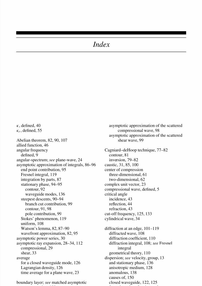
8/4/2019 Linear Elastic Waves (Cambridge Texts in Applied Mathematics) (John G. Harris) 0521643686
http://slidepdf.com/reader/full/linear-elastic-waves-cambridge-texts-in-applied-mathematics-john-g-harris 178/180
160 Index
dispersion ( cont. )open waveguide, 130, 131periodic structure, 18
eigenvalue problem, 122eigenfunction
continuous expansion, 139discrete or mode expansion, 134
eigenvalues, 123discrete and continuous, 145
eigenvalues and eigenfunctionsdiscrete, 122discrete and continuous, 131
eikonal equation, 30, 148energy relations, 5
kinetic energy density, dened, 6averaged for a closed waveguide mode, 126averaged for a plane wave, 23conservation law, 6, 127energy ux during critical refraction, 45energy ux during reection, 41energy ux, dened, 6energy in a band of frequencies, 156equipartition of energy, 126for a transient plane wave, 22for the exural motion equation, 128for the Klein–Gordon equation, 128internal energy density, dened, 6
equations of motion, 1–6boundary conditions, 2dilitational motion, 2one-dimensional, 3rotational motion, 2two-dimensional, 4
antiplane motion, 4inplane motion, 4
extinction theorem, 75
fareldcompact source, 61, 65of an edge, 114
Fermat’s principle, 101exural motion equation, 48, 127, 157Fourier transform
space, 10three-dimensional, 58time, 7
frequencydened, 9local, 155
Fresnel integral, 109, 116–119
gamma function, 87Gaussian beam; see plane-wave
representations, 25geometrical theory of diffraction;
see diffraction at an edge, 111
Green’s function, 60, 62method of images, 68
Green’s tensor, 58, 62
correct and incorrect, 66elastic uid, 74stress, 60three-dimensional, 58
guided waves; see waveguide, 121
Helmholtz theorem, 5
initial value problem, 157inner expansion; see matched asymptotic
expansion, 71integral equations, 67, 76integral representation
scattering problem, 65–67source problem, 64–65
JWKB asymptotic expansioneigenvalue problem, 148rays and modes, 147
Klein–Gordon equation, 127, 150, 157
Lagrangian density, 126Lamb’s problem; see buried harmonic line of
compression, 82Laplace transform
time, 7two-sided, 78
leaky wave; see waveguide, open, 146limiting absorption, principleof, 62–63, 65, 135
and the Wiener–Hopf method, 104–108
outgoing wave, 58, 59, 79line of compression; see center of compression,
83longitudinal wave; see compressional, 22Love wave; see waveguide, open, 131
matched asymptotic expansion, 112–116boundary layer, 109, 111, 113inner, outer coordinates, 71, 114inner, outer expansion, 71, 114
matching, 115Schrodinger equation, 114stretching transformation, 114
neareld of an edge, 72, 104, 110, 113
outer expansion; see matched asymptoticexpansion, 71
outgoing wave; see limiting absorption, 59
partial waves, 17, 123, 140, 145periodic structure, 15–18
effective wavenumber, 18

8/4/2019 Linear Elastic Waves (Cambridge Texts in Applied Mathematics) (John G. Harris) 0521643686
http://slidepdf.com/reader/full/linear-elastic-waves-cambridge-texts-in-applied-mathematics-john-g-harris 179/180
Index 161
phase matching, 39–40phase, its meaning, 29plane wave
homogeneous, 22inhomogeneous or evanescent, 22, 43, 96time-dependent, 20time-harmonic, 22
plane-wave representations, 24–28cylindrical wave, 28, 140Gaussian beam, 24in an open waveguide, 142, 146spherical wave, 27, 28waves scattered from a surface, 84
Poisson summation formula, 11polarization
change in a ray expansion, 33dened, 20
potentials, displacement, 5scalar potential, 5vector potential, 5
propagation matrix, 16
radiation conditions, 65; see limitingabsorption, 65
ray; see asymptotic ray expansion, 30dened, 30fan of diffracted rays, 110ray tube, 33rays and modes, 146
Rayleigh wave, 48–52, 96, 101Rayleigh function, 51Rayleigh equation, 49time-harmonic, 49transient, 50
two-sided wave, 51reciprocity, 57reection
antiplane shear coefcient, 44antiplane shear wave, 42compressional coefcient, 40compressional wave, 38from a layer, 133from a plate in a uid, 47inplane shear coefcient, 40
inplane shear wave, 38refractionantiplane shear coefcient, 44antiplane shear wave, 42interfacial wave, 45two-sided wave, 46
scalar potential; see potentials,displacement, 5
scatteringBragg, 17from a lumped mass, 13from a strip, 67
from an elastic inclusion, 72scattering matrix, 14
shear wave, dened, 5
signaling problem, 151–157dened, 24slowness
dened, 20surface, 39, 44vector, 20, 39
Sommerfeld transformation, 27, 59, 84, 96, 142spherical wave, 34standing wave, dened, 9stationary phase; see asymptotic approximation
of integrals, 94steepest descents; see asymptotic
approximation of integrals, 90strain tensor, dened, 2stress tensor, dened, 1surface wave; see Rayleigh wave, 51
guided by an impedance boundary, 51
Tauberian theorem; see Abelian theorem, 82traction, dened, 1transforms, Fourier and Laplace; see Fourier
transform, Laplace transform, 6dened, 6–10
transmission coefcient; see refraction, 44transmission matrix, 15transport equation, 30, 149transverse resonance principle, 124transverse wave; see shear, 22
uniqueness in an unbounded region, 63,68–72
edge conditions, 69, 104, 107no edges, 68
vector potential; see potentials, displacement, 5velocity
energy transport, 22, 24, 125fastest, 137group; see dispersion, 18
and stationary phase, 137group lines, 155
kinematic theory, 154kinetic theory, 156periodic structure, 18propagation of angular frequencies,
153–157propagation of information, 151propagation of wavenumbers, 153waveguide mode, 125
phaselocal, 155phase lines, 155waveguide mode, 125
vibration, not a wave, 11

8/4/2019 Linear Elastic Waves (Cambridge Texts in Applied Mathematics) (John G. Harris) 0521643686
http://slidepdf.com/reader/full/linear-elastic-waves-cambridge-texts-in-applied-mathematics-john-g-harris 180/180
162 Index
Watson’s lemma; see asymptoticapproximationof integrals, 87
wave kinematics, dened, 20
wavefrontcurvature, 32dened, 30plane, spherical, etc., 20
waveguideclosed, 121
evanescent mode, 135excitation, 134–139harmonic excitation, 134mode expansion, 134transient excitation, 135
laterally inhomogeneous, 146mode, 122open, 129
excitation, 139–146leaky modes, 146modal representation, 144
plane-wave representation, 142, 146ray representation, 141, 145wavelength, dened, 9wavenumber
complex, 22dened, 8effective, periodic structure, 18lateral, 122local, 155transverse, 122
wavevectordened, 22real and complex, 22
Wiener–Hopf method, 104–108