linear optimization of district heating systems · oppgraderte modulen er mer realistisk i forhold...

LINEAR OPTIMIZATION OF DISTRICT HEATING SYSTEMS

Description of an upgraded district heating module for eTransport

ZEN REPORT No. 9 – 2018

Karoline Kvalsvik and Hanne Kauko | Christian Michelsen Research / SINTEF Energy

ZEN REPORT No. 9 ZEN Research Centre 2018

2

ZEN Report No. 9

Karoline Kvalsvik (Christian Michelsen Research)

Hanne Kauko (SINTEF Energy)

Upgraded district heating module for eTransport

Keywords: district heating, modeling, planning tools, linear optimization

ISBN 978-82-536-1596-7

Norwegian University of Science and Technology (NTNU) | www.ntnu.no

SINTEF Building and Infrastructure | www.sintef.no

https://fmezen.no



3

Preface

Acknowledgements

This report has been written within the Research Centre on Zero Emission Neighbourhoods in Smart

Cities (FME ZEN). The authors gratefully acknowledge the support from the Research Council of

Norway, the Norwegian University of Science and Technology (NTNU), SINTEF, the municipalities

of Oslo, Bergen, Trondheim, Bodø, Bærum, Elverum and Steinkjer, Trøndelag county, Norwegian

Directorate for Public Construction and Property Management, Norwegian Water Resources and

Energy Directorate, Norwegian Building Authority, ByBo, Elverum Tomteselskap, TOBB, Snøhetta,

Tegn_3 , Asplan Viak, Multiconsult, Sweco, Civitas, FutureBuilt, Hunton, Moelven, Norcem,

Skanska, GK, Caverion, Nord-Trøndelag Elektrisitetsverk (NTE), Smart Grid Services Cluster,

Statkraft Varme, Energy Norway and Norsk Fjernvarme.

The Research Centre on Zero Emission Neighbourhoods (ZEN) in Smart Cities

The ZEN Research Centre develops solutions for future buildings and neighbourhoods with no

greenhouse gas emissions and thereby contributes to a low carbon society.

Researchers, municipalities, industry and governmental organizations work together in the ZEN

Research Centre in order to plan, develop and run neighbourhoods with zero greenhouse gas

emissions. The ZEN Centre has nine pilot projects spread over all of Norway that encompass an area

of more than 1 million m2 and more than 30 000 inhabitants in total.

In order to achieve its high ambitions, the Centre will, together with its partners:

• Develop neighbourhood design and planning instruments while integrating science-based

knowledge on greenhouse gas emissions;

• Create new business models, roles, and services that address the lack of flexibility towards

markets and catalyze the development of innovations for a broader public use; This

includes studies of political instruments and market design;

• Create cost effective and resource and energy efficient buildings by developing low

carbon technologies and construction systems based on lifecycle design strategies;

• Develop technologies and solutions for the design and operation of energy flexible

neighbourhoods;

• Develop a decision-support tool for optimizing local energy systems and their interaction

with the larger system;

• Create and manage a series of neighbourhood-scale living labs, which will act as

innovation hubs and a testing ground for the solutions developed in the ZEN Research

Centre. The pilot projects are Furuset in Oslo, Fornebu in Bærum, Sluppen and Campus

NTNU in Trondheim, an NRK-site in Steinkjer, Ydalir in Elverum, Campus Evenstad,

NyBy Bodø, and Zero Village Bergen.

The ZEN Research Centre will last eight years (2017-2024), and the budget is approximately NOK

380 million, funded by the Research Council of Norway, the research partners NTNU and SINTEF,

and the user partners from the private and public sector. The Norwegian University of Science and

Technology (NTNU) is the host and leads the Centre together with SINTEF.

https://fmezen.no

@ZENcentre

FME ZEN (page)


4

Abstract eTransport is a linear optimization tool for evaluating energy supply alternatives for building areas.

This report describes an improved, more realistic district heating (DH) module that has been

developed for eTransport. The new module includes several improvements as compared to the

previous module:

Varying mass flow that depends on the heat load, as opposed to constant mass flow.

Pressure included as a variable, with certain limits for minimum pressure and minimum pressure

drop at the loads.

Calculation of pumping power is included in the module, and pumping power due to pressure

losses in pipes and at loads is included in the objective function

A more realistic calculation of heat losses included, and the heat losses are included in the heat

load

The module allows supply flow to both directions in a pipe; a property which is relevant when

more heat sources are present in a DH grid. This feature is however yet to be tested properly.

The report presents the main equations required for mathematical description of a district heating

system are presented, followed by the approach taken for linear representation of these equations,

required for eTransport. The report includes a brief evaluation of the module using a simple test

network, and discusses the simplifications and limitations of the present module, giving suggestions

for further improvements.


5

Sammendrag Fjernvarme er en viktig muliggjørende teknologi i det grønne skiftet. Fjernvarme kan nyttiggjøre

energi som ellers ville gått til spille, slik som gjenvunnet varme fra avfallsforbrenning og

industriprosesser; eller mindre spillvarmekilder tilgjengelig i byer, slik som datasentre og store

matvarebutikker. Ved hjelp av et fjernvarmesystem kan slike kilder anvendes til oppvarming av

boliger og næringsbygg. Med et godt samspill med kraftnettet bidrar fjernvarme i tettbygde strøk til å

avlaste kraftnettet og tilgjengeliggjøring elektrisitet til andre formål enn til oppvarming.

Bygging av et fjernvarmesystem krever store investeringer i startfasen, og dermed er det viktig å vite

hvilke energikilder man bør velge til et gitt område for å minimere tilbakebetalingstiden. Det er derfor

vanlig å bruke planleggingsverktøy for sammenlikning av ulike energiforsyningsalternativer til

området. eTransport er et slikt verktøy, lagd av SINTEF Energi i 2006. Verktøyet skal oppgraderes og

videreutvikles i FME ZEN. eTransport omfatter flere energibærere, og finner den optimale måten til å

drifte energisystemet, samt en optimal ekspansjonsplan i et geografisk definert område. I mange

tilfeller vil det være konkurransen mellom ulike energibærere: behovet for oppvarming kan dekkes av

elektrisitet eller av et fjernvarmesystem og varme kan genereres fra kilder. eTransport beregner de

årlige driftskostnadene for ulike energisystemdesign, og sender disse til en investeringsmodell som

finner en optimal ekspansjonsplan.

Denne rapporten beskriver en oppgradering av fjernvarmemodulen i eTransport. I den tidligere

versjonen av eTransport var modulen for beskrivelse av et fjernvarmesystem svært forenklet. Den

oppgraderte modulen er mer realistisk i forhold til beregning av massestrøm, varmetap, trykktap og

pumpearbeid. Modulen tillater dessuten forsyning av varme i begge retninger i et rør, noe som kan

være aktuelt i et varmenett som utnytter flere, distribuerte varmekilder. eTransport et lineært

optimalisverktøy, og rapporten presenterer den valgte tilnærmingen for lineær formulering av de

viktigste likningene for beskrivelse av et fjernvarmesystem.


6

Contents

Preface .............................................................................................................................................3

Abstract .............................................................................................................................................4

Sammendrag .............................................................................................................................................5

1 Introduction ..........................................................................................................................7

1.1 A notion on the types of components in eTransport ............................................................7

2 Mathematical description of a DH system ...........................................................................8

2.1 Heat flow..............................................................................................................................8

2.2 Heat losses ...........................................................................................................................8

2.3 Pressure drop and pumping power .......................................................................................9

3 Linear representation of a DH system ...............................................................................12

3.1 Heat flow............................................................................................................................12

3.2 Heat losses .........................................................................................................................14

3.3 Pressure drop......................................................................................................................15

3.4 Pumping power ..................................................................................................................18

3.5 The objective function for the DH model ..........................................................................21

4 Evaluation of the new module ...........................................................................................22

5 Conclusions and future work .............................................................................................23

References 25

A1. Appendix 1: Parameters, variables and sets ....................................................................................26

A2. Appendix 2: Objective function and the constraints........................................................................29


7

1 Introduction eTransport is an economical tool for finding the most optimal energy supply alternative for a building

area, capable of evaluating several possible investments and energy flows for periods of several years

in only a few seconds. Being a linear optimization model, a global optimum is guaranteed. Several

types of energy carriers, as well as conversion possibilities between them, are included: electricity,

gas, district heating (DH) and hydrogen. Moreover, several primary energy sources, with penalties

depending on their costs and emissions are included: gas, biomass, municipal waste and oil, to

mention a few. The primary energy sources are converted into the desired energy carriers, in this case

heated DH water, through the use of for instance boilers or combined heat and power plants, in order

to supply energy for the building area in question.

This report describes the upgrading of the DH module in eTransport. The previous DH module had

several important weaknesses:

It had no variable for pressure, which is crucial for acceptable design and operation.

The mass flow was set to a constant.

It would allow any return temperature at a load.

The effect of pipe length on heat and pressure losses was not included

Calculation of heat loss was incorrect, in particular for the return line.

The goal for the development of the new DH module has been to address these drawbacks. This

document is organized as follows: Chapter 2 introduces the governing, physically correct equations

needed to describe a DH system. Chapter 3 presents the chosen approach for linear representation of

these equations, including suggestions for future improvements. Chapter 4 shows results from

evaluation of the implemented model, while Chapter 5 concludes the report and gives suggestion for

further work.

1.1 A notion on the types of components in eTransport

eTransport has been programmed using AMPL (A Mathematical Programming Language), which is a

programming language for mathematical programming, particularly suited for formulating

optimization problems (Fourer 2003). Being a mathematical programming language implies that the

syntax resembles to a large degree the actual mathematical formulations.

AMPL has the following fundamental components:

Sets are used for indexing, that is, a variable or a parameter may have different value for

different elements in a set. In a DH system, typical sets are e.g. the junction points (nodes), the

load points, and production (source) points.

Parameters are elements whose value is known or can be calculated at the start of a calculation.

A parameter may be defined as an integer.

Variables are elements whose value is not known beforehand and which may vary during the

simulation. Variables are often subject to a constraint or objective. A variable may be defined

as binary.

Constraints are the equations determining the behaviour of variables. These equations need to

be linear in terms of variables, however nonlinear equations may be applied for parameters.


8

Objectives or objective functions describe the function that the user wishes to minimize. This

function is generally a summation of different variables over certain sets, weighed with a certain

penalty. In eTransport, each submodel (e.g. the DH module, gas supply, electricity supply) has

one objective function, which will be passed on and minimized by the universal model.

The sets, parameters and variables included in the DH module are listed and explained in Appendix

A1. The objective function and the constraints are listed in Appendix A2.

2 Mathematical description of a DH system

A DH grid in any model is represented by a set of equations. This chapter describes the main variables

the DH model must be able to calculate at an appropriate accuracy – the transported heat, heat loss,

pressure drop and required pump work – and presents the exact equations representing these variables.

2.1 Heat flow

Transport of heat is the most important function of a DH system, and the simplest DH model one

could imagine would simply involve heat flowing from a source to one or several sinks. This is the

sole purpose of DH and this variable must thus be included in the model. Ideally, the heat flow at

sources and loads should be modelled as:

�̇� = �̇�𝑐𝑝(𝑇𝑖𝑛 − 𝑇𝑜𝑢𝑡) (1)

where �̇� is the heat flow (in [kW]); �̇� the volume flow of water (in [m3/s]); cp is the specific heat

capacity of water (here given in [kJ/(m3∙K)]); and Tin and Tout are the temperatures in and out (in [°C]),

respectively.

The total heat flowing in and out of a node should the equal:

∑ �̇�𝑖𝑖 = ∑ �̇�𝑖𝑐𝑝𝑇𝑖𝑖 = 0 (2)

Here, �̇�𝑖 is a heat flow in or out of the node, and �̇�𝑖 and 𝑇𝑖 are the volume flow and temperature level

of each stream in °C (minimum temperature in the system is set to be > 0). Volume flow and hence

heat flowing out of a node are considered negative. The summation is hence over all heat flows in and

out of a node.

Moreover, the sum of water flowing into each node should the zero, that is

∑ �̇�𝑖𝑖 = 0 (3)

where �̇�𝑖 is a mass of water flowing in or out of the node. Again, streams flowing out of the node are

considered negative. Assuming constant water density, which is very close to the truth, Equation (3)

can be formulated in terms of volume flow as

∑ �̇�𝑖𝑖 = 0 (4)

2.2 Heat losses

Heat losses is the second most important variable to consider. Heat losses may constitute 10-25 % of

the heat supplied to the grid, and have thus substantial impact on primary energy demand and

emissions seen from a supplier side. It will be very important to know whether 3 or 25 % losses are

expected, as the heat supply must be 3.1 or 33 % higher than the heat demand, respectively. Models


9

not including heat losses could thus be far off in estimating required heat supply and associated costs.

Estimating the losses as a constant percentage of the heat demand could also be a costly mistake to

make.

The actual amount of heat losses varies significantly from system to system, depending on the supply

temperature level, heat transport distance and level of insulation in pipes. In new areas with well-

insulated houses, high heat demand density (heat demand per unit area) and low supply temperature

level, the heat losses per metre may be low; however the relative heat losses may be high due to the

low heat demand. More detailed and physically correct model studies have shown losses of only 3-5 %

for a well-insulated low temperature grid (Kauko, 2018). Hence, the effect of insulation, temperature

level and distance between the loads must be included for correct estimation of the heat losses.

Heat losses depend on the geometry and insulation of the pipe, and for twin pipes often used for

smaller pipe diameters in DH systems, rather complex formulae are applied (see e.g. (Wallentèn,

1991)). The principle for calculating heat losses can be well understood by considering the simpler

equation for heat loss for a single, circular, concentric pipe:

�̇�𝑙𝑜𝑠𝑠 = 2𝜋𝐿𝑘𝑇𝑤𝑎𝑡𝑒𝑟−𝑇𝑎𝑚𝑏

ln(𝐷𝑜

𝐷𝑖⁄ )

(5)

In this equation, L is the pipe length, k the thermal conductivity of the insulation (also known as the λ-

value), Do and Di are the outer and inner diameters of the pipe and Twater and Tamb are the temperatures

of the water and the ambient, respectively.

2.3 Pressure drop and pumping power

Pressure drop in pipes and the associated pumping power are less important for the total energy

demand in a DH system as the pumping power is typically one order of magnitude lower than the heat

loss and two orders of magnitude lower than the heat demand. Nevertheless, pressure loss is the

determining factor for dimensioning of pipes and hence important considering investment costs. Pipes

and other hydraulic equipment are designed for a certain maximum pressure, which depends on the

pipe diameter and maximum mass flow. In the DH system in Trondheim, the pressure should never

exceed 10 bar. A model should preferably deliver a warning if the maximum pressure is exceeded (not

included in the present module). The pipe pressure can be reduced by increasing the diameter of the

pipes, however higher pipe diameter yields higher investment costs and heat losses. Hence the lowest

possible pipe diameter is generally chosen, still capable of delivering the required maximum mass

flow during peak heating demand periods.

The pressure drop dp in a circular pipe can be calculated using the Darcy-Weisbach equation

(Fredriksen & Werner, 2014):

𝑑𝑝 = 𝑓𝜌𝐿

2𝐷�̇�2 (6)

where f is a friction factor, L the pipe length, D the pipe diameter and ρ the fluid density. The pipes are

normally designed based on a maximum allowed pressure drop per metre at a given maximum water


10

flow, �̇�𝑚𝑎𝑥, known as the the R-value. Using the R-value, Equation (6) can be simplified to

(Fredriksen & Werner, 2014):

𝑑𝑝 = 𝑅𝐿 (�̇�

�̇�𝑚𝑎𝑥)

2

(7)

Here, a constant friction factor has been assumed, which is a valid assumption under normal

operational conditions. The main advantage of this equation is that it only contains parameters that the

industry is familiar with.

Pressure drop is what causes the demand for pumping water. The power demand P of a pump is given

by:

𝑃 =𝑑𝑝�̇�

𝜂=

𝑅𝐿

𝜂(

�̇�

�̇�𝑚𝑎𝑥)

2

�̇� ∝ �̇�3 (8)

where dp is the pressure lift of the pump (in [Pa]), �̇� the volume flow through the pump and η is the

pump efficiency. In reality, η is a function of the volume flow and the pressure lift. Modelling it as

constant has been tested to be a fair approximation, also in more complex models (Kauko, Kvalsvik et

al. 2017, Kauko, Kvalsvik et al. 2018). It is noted that the pump work represents an electricity demand

and should perhaps be converted to an electricity demand of the heating module, not unlike the heat

and electricity conversion in the already existing heat pump model.

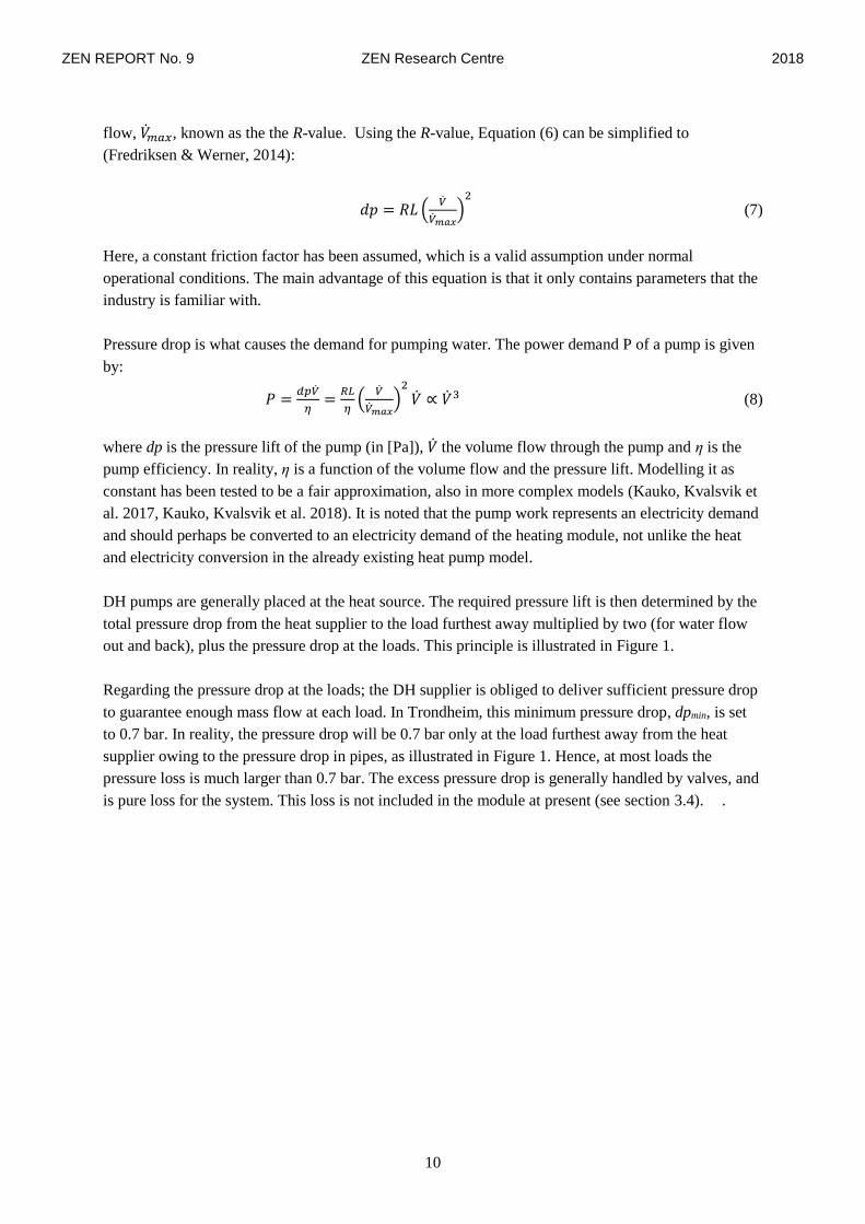
DH pumps are generally placed at the heat source. The required pressure lift is then determined by the

total pressure drop from the heat supplier to the load furthest away multiplied by two (for water flow

out and back), plus the pressure drop at the loads. This principle is illustrated in Figure 1.

Regarding the pressure drop at the loads; the DH supplier is obliged to deliver sufficient pressure drop

to guarantee enough mass flow at each load. In Trondheim, this minimum pressure drop, dpmin, is set

to 0.7 bar. In reality, the pressure drop will be 0.7 bar only at the load furthest away from the heat

supplier owing to the pressure drop in pipes, as illustrated in Figure 1. Hence, at most loads the

pressure loss is much larger than 0.7 bar. The excess pressure drop is generally handled by valves, and

is pure loss for the system. This loss is not included in the module at present (see section 3.4). .


11

Figure 1:

Illustration of the pressure drop as a function of distance from a heat central, and the pressure losses occurring at

loads


12

3 Linear representation of a DH system

As shown in Chapter 2, all the main equations representing a DH system are non-linear, apart from the

mass conservation and heat loss equations. The challenge then is to represent a DH system using only

linear equations; and the chosen solutions to describe heat flow, heat losses, pressure drop and

pumping power are presented in this chapter. Section 3.5 summarizes the chapter and introduces the

final objective function for the DH model, to be passed on to the universal model.

3.1 Heat flow

The mass balance (Equations (3) and (4)) is linear and used as it is, with one modification to be

outlined in section 3.3. To preserve energy while having varying conditions and linear equations,

Equation (2) for energy balance in each node, was changed into

∑ �̇�𝑙𝑒𝑠𝑠,𝑖𝑖 = 0 (9)

with the summation being again over all the in- and outgoing flows from a node, with negative sign

for outgoing flows. Now, �̇�𝑙𝑒𝑠𝑠 is a new variable defined as the heat removed from the water after it

left the heat central. That is,

�̇�𝑙𝑒𝑠𝑠 = �̇�𝑐𝑝(𝑇𝑠𝑢𝑝𝑝𝑙𝑦 − 𝑇𝑤𝑎𝑡𝑒𝑟) (10)

Where 𝑇𝑠𝑢𝑝𝑝𝑙𝑦 is the supply temperature at the production site, and 𝑇𝑤𝑎𝑡𝑒𝑟 is the water temperature at

the node in question. Neither of these is a variable, and hence the challenge with the nonlinear energy

balance equation is avoided. Notice that 𝑇𝑤𝑎𝑡𝑒𝑟 is actually never calculated in the model – equation

(10) is rather given as an exact definition for �̇�𝑙𝑒𝑠𝑠.

At the loads, with heat demand �̇�𝑙𝑜𝑎𝑑, we require

�̇�𝑙𝑒𝑠𝑠 + �̇�𝑙𝑜𝑎𝑑 + �̇�𝑑𝑒𝑓𝑖𝑐𝑖𝑡 ≤ �̇�𝑐𝑝(𝑇𝑠𝑢𝑝𝑝𝑙𝑦 − 𝑇𝑟𝑒𝑡𝑢𝑟𝑛) (11)

Where 𝑇𝑟𝑒𝑡𝑢𝑟𝑛 is the return temperature from the load, and �̇�𝑑𝑒𝑓𝑖𝑐𝑖𝑡 is the heat demand that could not

be delivered at the load with the given heat load, losses, temperature limits and flow. As seen from this

equation, the heat demand of the load, as well as the possible heat deficit, is added to the variable

�̇�𝑙𝑒𝑠𝑠. �̇�𝑙𝑒𝑠𝑠 is thus much higher in the return pipes than in the supply pipes. The heat demand at each

load point is a variable, received as an input from the universal model.

Based on Equation (11), the water flow must be so large that the demand is covered and the

temperature changing within a realistic interval. If these limits are parameters, this is a linear equation.

In the DH model, the return temperature was set to a constant value, making Equation (11) linear. In

reality, the return temperature depends on the inlet temperature, as well as the conditions for heat

exchange at the load. As the inlet (supply) temperature was set constant, it is a fair simplification to set

the return temperature to be constant. A more sophisticated approach could be to make the return

temperature a function of ambient and/or inlet temperature, which is quite realistic. The return

temperature could also be calculated differently for each load, time step and/or season as well, if

desirable.


13


14

3.2 Heat losses

Heat losses in DH systems are generally given as heat loss per metre pipe, and this value is available

from pipe producers for a water temperature of 50 °C for a certain type of pipe. The ambient

temperature was assumed to be equal to 10°C. With these simplifications, Equation (5) could be

written as:

�̇�𝑙𝑜𝑠𝑠 = 𝐾(𝑇𝑤𝑎𝑡𝑒𝑟 − 𝑇𝑎𝑚𝑏)𝐿 (12)

Where 𝑇𝑎𝑚𝑏 is the ambient temperature, 𝑇𝑤𝑎𝑡𝑒𝑟 is the momentary (unknown) DH water temperature

and the heat loss factor K (in [MW/(K*m]) is defined as

𝐾 =�̇�𝑙𝑜𝑠𝑠 𝑎𝑡 50°𝐶

(50−10)°𝐶 (13)

Equation (12) represents a straightforward approach for calculating heat losses, when assuming that

the water temperature does not change along the pipe. Keeping the temperature constant is the same as

assuming no heat loss; however, heat losses in the supply line do not, and should not, change the

temperature significantly. Hence the heat loss in the supply line can be modelled as proportional to a

constant 𝑇𝑠𝑢𝑝𝑝𝑙𝑦; i.e., setting 𝑇𝑤𝑎𝑡𝑒𝑟 = 𝑇𝑠𝑢𝑝𝑝𝑙𝑦, with only minor errors occurring.

As an example, assuming an ambient temperature of 25 °C, supply temperature of 65 °C, and a

temperature at the load of 63 °C, the ratio of the modelled and real heat losses should be about

�̇�𝑙𝑜𝑠𝑠,𝑀𝑜𝑑𝑒𝑙

�̇�𝑙𝑜𝑠𝑠,𝑅𝑒𝑎𝑙

∝𝑇𝑠𝑢𝑝𝑝𝑙𝑦 − 𝑇𝑎𝑚𝑏

𝑇𝑤𝑎𝑡𝑒𝑟 − 𝑇𝑎𝑚𝑏≈

65 − 25

64 − 25= 102.6%

In this estimate, 64 °C was used for 𝑇𝑤𝑎𝑡𝑒𝑟, representing the average temperature between the source

and the load. The resulting error was only 3 %, even though this example calculation represents one

of the highest errors that could occur. Most of the losses occur during the winter, thus, a more typical

situation would be 𝑇𝑠𝑢𝑝𝑝𝑙𝑦 of 100 °C, 𝑇𝑎𝑚𝑏 of 0 °C, and the supply water arriving at the load at 99°C.

This would give an error of only ~0.5 %.

In the model, there is no separate variable for heat loss, but the losses are included in the �̇�𝑙𝑒𝑠𝑠-

variable at the end of each pipe (i,j) in the supply line:

�̇�𝑙𝑒𝑠𝑠(𝑖, 𝑗, 𝑒𝑛𝑑) = �̇�𝑙𝑒𝑠𝑠(𝑖, 𝑗, 𝑠𝑡𝑎𝑟𝑡) + 𝐾(𝑇𝑠𝑢𝑝𝑝𝑙𝑦 − 𝑇𝑎𝑚𝑏)𝐿(𝑖,𝑗) (14)

Where �̇�𝑙𝑒𝑠𝑠(𝑖, 𝑗, 𝑠𝑡𝑎𝑟𝑡) and �̇�𝑙𝑒𝑠𝑠(𝑖, 𝑗, 𝑒𝑛𝑑) are the values for �̇�𝑙𝑒𝑠𝑠 at the start and end of pipe (i,j),

respectively, 𝐿(𝑖,𝑗) is the length of the pipe. A limitation in this approach is that heat losses are

calculated and allocated for a pipe even if there is no flow in the pipe. An improved model should

have an approach to prevent this.

Heat losses in the return line are very small, and in any case much smaller than the losses in the supply

pipes (Dalla Rosa, 2011). Losses in the return pipe can even be negative in twin pipes, as heat leaks

from the supply to the return line. Thus, it was decided that the model should have heat loss free return

lines. Even if this approach is somewhat wrong, recall that the approach to model heat losses is based


15

on using typical total heat losses in the grid per metre. Ergo the total heat loss will be correctly

calculated if, the heat loss in the return lines are zero, and the return losses are moved to the supply

line. The heat suppliers in the modelled grid receives the value �̇�𝑙𝑒𝑠𝑠 in the return line, which then

contains the total amount of heating required: heat demand at the load plus heat losses (see Equation

(11), without the need to multiply the temperature difference with the mass flow at the source. In this

way, another non-linear equation is avoided.

To ensure the temperature at the loads is sufficiently high, a minimum temperature for the water

arriving at the load, 𝑇𝑠𝑢𝑝𝑝𝑙𝑦,𝑚𝑖𝑛, was defined. The model must thus demand that

�̇�𝑙𝑒𝑠𝑠 ≤ �̇�𝑐𝑝(𝑇𝑠𝑢𝑝𝑝𝑙𝑦 − 𝑇𝑠𝑢𝑝𝑝𝑙𝑦,𝑚𝑖𝑛) (15)

This equation sets the temperature drop due to heat loss in pipes to be within an allowed range.

3.3 Pressure drop

The most important function of the pressure drop model is to provide a motivation to reduce the water

flow – remember that the pressure drop dp is proportional to the 2nd power and pumping power to the

3rd power of water flow, as shown by Equations (6) and (8). Apart from this, the maximum limits for

pressure is what determines the sizing of pipes and thereby investment costs of a system.

Pressure drop in pipes is a linear function of the pipe length and should have a value at each end of

every pipe. All pressures at one point (where more pipe ends are connected) must also be equal for

flow in the same direction (supply or return), but the absolute value for pressure in the supply and

return line differ significantly (remember Figure 1). Since the pipe length and water flow out and back

must be equal, i.e., the pressure drop in the supply and return line must be equal, it is sufficient to

calculate the pressure drop in the return line to find the entire pressure drop in a grid. The lowest

pressure value can be constant, whereas the highest value varies depending on the water flow in the

pipes.

The quadratic dependence of pressure drop on the water flow could be approximated by a piecewise

linear function; however, this would require different piecewise functions for all pipes. It was thus

decided to use dimensionless variables which will be in the range 0-1 (later this was changed to -1 to

+1, but this is a mere extension of what is described here). Using

�̇�∗ =�̇�

�̇�𝑚𝑎𝑥 and 𝑑𝑝∗ =

𝑑𝑝

𝑑𝑝𝑚𝑎𝑥=

𝑑𝑝

𝑅𝐿= (

�̇�

�̇�𝑚𝑎𝑥 )

2

= �̇�∗2 (16)

A piecewise linear pressure drop function for all pipes and water flows was obtained and is given by

𝑑𝑝∗ =

0.24 �̇�∗, �̇�∗ < 0.316

�̇�∗ − 0.24, 0.316 ≤ �̇�∗ ≤ 0.657

1.7�̇�∗ − 0.7, 0.657 < �̇�∗

(17)


16

which was modelled as

𝑑𝑝∗ ≥ { 0,24 �̇�∗

�̇�∗ − 0.241.7�̇�∗ − 0.7

} (18)

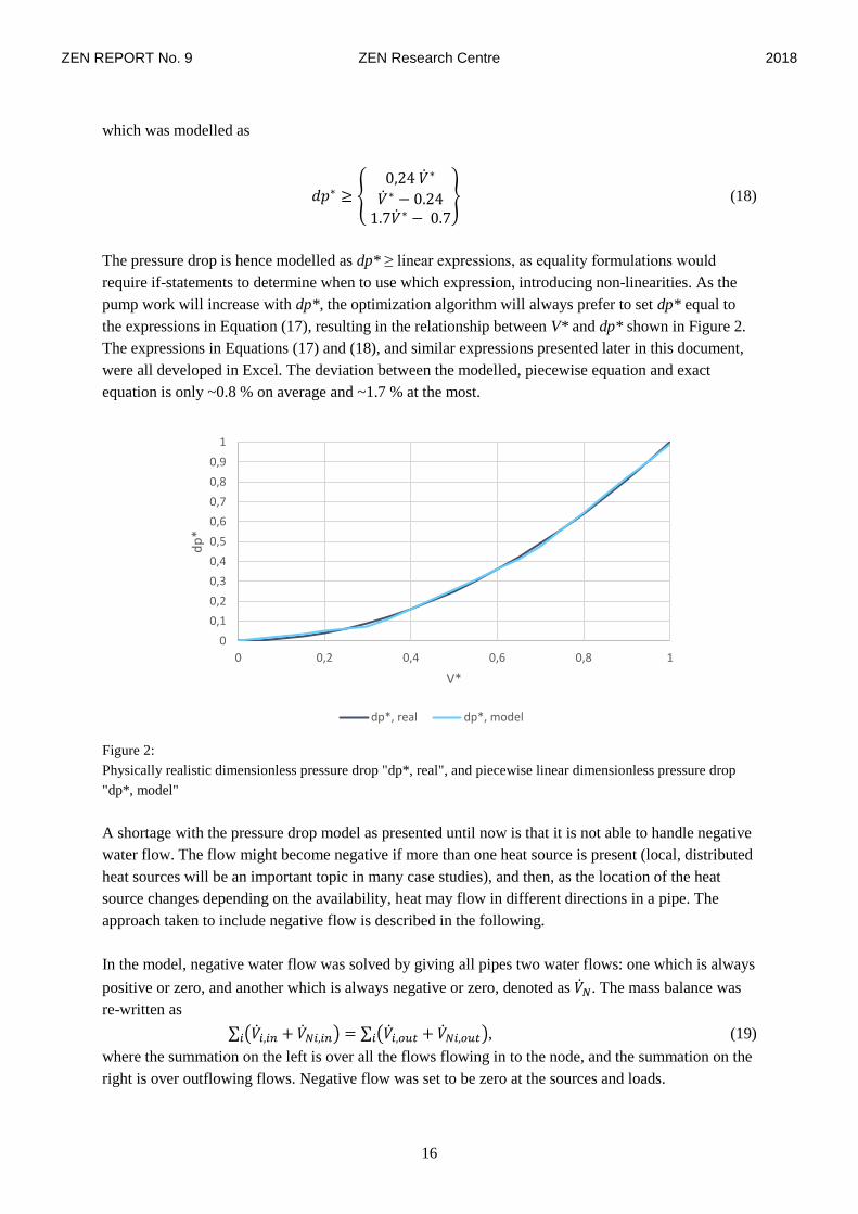
The pressure drop is hence modelled as dp* ≥ linear expressions, as equality formulations would

require if-statements to determine when to use which expression, introducing non-linearities. As the

pump work will increase with dp*, the optimization algorithm will always prefer to set dp* equal to

the expressions in Equation (17), resulting in the relationship between V* and dp* shown in Figure 2.

The expressions in Equations (17) and (18), and similar expressions presented later in this document,

were all developed in Excel. The deviation between the modelled, piecewise equation and exact

equation is only ~0.8 % on average and ~1.7 % at the most.

Figure 2:

Physically realistic dimensionless pressure drop "dp*, real", and piecewise linear dimensionless pressure drop

"dp*, model"

A shortage with the pressure drop model as presented until now is that it is not able to handle negative

water flow. The flow might become negative if more than one heat source is present (local, distributed

heat sources will be an important topic in many case studies), and then, as the location of the heat

source changes depending on the availability, heat may flow in different directions in a pipe. The

approach taken to include negative flow is described in the following.

In the model, negative water flow was solved by giving all pipes two water flows: one which is always

positive or zero, and another which is always negative or zero, denoted as �̇�𝑁. The mass balance was

re-written as

∑ (�̇�𝑖,𝑖𝑛 + �̇�𝑁𝑖,𝑖𝑛)𝑖 = ∑ (�̇�𝑖,𝑜𝑢𝑡 + �̇�𝑁𝑖,𝑜𝑢𝑡)𝑖 , (19)

where the summation on the left is over all the flows flowing in to the node, and the summation on the

right is over outflowing flows. Negative flow was set to be zero at the sources and loads.

0

0,1

0,2

0,3

0,4

0,5

0,6

0,7

0,8

0,9

1

0 0,2 0,4 0,6 0,8 1

dp

*

V*

dp*, real dp*, model


17

Energy balance is valid as it is. Heat losses depend on temperature and are not affected by negative

flow but might be added at the wrong end of the pipe, hence be wrongly allocated; this has however no

effect on the overall energy balance. Pressure drop on the other hand introduces a larger problem.

Depending on the direction of the flow, the model might not know whether the pressure drop should

be added to the inlet or the outlet of the pipe; that is, whether

𝑝𝑜𝑢𝑡 = 𝑝𝑖𝑛 + 𝑑𝑝 (20)

or

𝑝𝑖𝑛 = 𝑝𝑜𝑢𝑡 + 𝑑𝑝 (21)

For negative water flows, a negative pressure drop, dpN, was therefore defined. The positive pressure

drop was forced to be zero for negative flows and force dpN to be zero for positive flows. Then

𝑝𝑜𝑢𝑡 = 𝑝𝑖𝑛 + 𝑑𝑝 + 𝑑𝑝𝑁 (22)

will always be valid. Forcing dpN to be zero if the water flow is larger than zero and not otherwise

again could introduce nonlinearity. dp is then defined in terms of the positive water flow (Equation

(17)), and dpN in terms of the negative flow analogously to Equation (17):

𝑑𝑝𝑁∗ ≥ {

0,24 �̇�𝑁∗

�̇�𝑁∗

+ 0.24

1.7�̇�𝑁∗

+ 0.71

} (23)

where again the * denotes the dimensionless values.

Equation (23) will however allow the model to make the pressure difference between the ends of a

pipe equal to zero. For negative flows, equation (17) requires that dp* should be set to any value ≥0,

which means it could be set equal to -dpN*, and thus cancel the pressure drop entirely. This is seen by

inserting 𝑑𝑝∗ = −𝑑𝑝𝑁∗ into Equation (22). Similarly, for positive flow, the model can choose to set

𝑑𝑝𝑁∗ = −𝑑𝑝∗, yielding same pressure in both ends of the pipe. Hence, a way to prevent dp* from

taking a value when �̇�∗ is zero, and dpN* from taking a value when �̇�𝑁∗ is zero is necessary. Realizing

that in terms of dimensionless variables, dp* is always smaller than �̇�∗, except from when they are

both zero or both one, the problem is solved by demanding that

𝑑𝑝∗ ≤ �̇�∗ (24)

and

𝑑𝑝𝑁∗ ≥ �̇�𝑁

∗ (25)

Figure 3 visualizes the allowed range for dp* as described above. In the figure, the following

equations are included:

The green line represents the ideal dp*, as calculated from Equation (7);

The black line represents the piecewise linear representation of dp* based on Equations (18)

and (23)

The black dashed line represents the equality 𝑑𝑝∗ = �̇�∗


18

The blue solid line (c) represents the equality 𝑑𝑝∗ = 0.24 �̇�∗

The blue dashed line (b) represents the equality 𝑑𝑝∗ = �̇�∗ + 0.24

The blue dotted line (a) represents the equality 𝑑𝑝∗ = 1.7�̇�∗ + 0.71

The pressure drop must always be on or between the blue dashed lines, by inequality constraints. The

positive pressure drop must be in the region between the black dashed line and the blue lines in the

first quadrant for positive flow, and zero otherwise, whereas the negative pressure drop must be

between the black dashed line and the blue lines in the third quadrant for negative flows, and zero

otherwise. These areas are marked yellow.

Figure 3:

Modelling dimensionless pressure drop dp* based on dimensionless water flow V*, limiting dp* and dpN* to be

in the yellow areas.

3.4 Pumping power

Calculating the pressure drop in itself is only important for ensuring that the pressure does not exceed

the allowable values. What is more interesting from an energy-economic perspective is to estimate the

required pumping power. The calculation is divided into two parts: the required pumping power due to

pressure drop in pipes, and the required power due to pressure drop at loads.

Pumping power due to pressure losses in pipes

Pumping power is calculated as a product of the pressure drop and the volume flow, as shown by

Equation (8). There is no linear function to imitate the behaviour of the product of two variables;

however, it is possible to represent non-linear relationships in a linear model by combining several

equations. Therefore, a non-dimensional pumping power was defined in a similar manner as was done

for pressure:


19

𝑃∗ =𝑃

𝑃𝑚𝑎𝑥 = 𝑃

𝜂

𝑅𝐿�̇�𝑚𝑎𝑥=

𝑅𝐿�̇�3

𝜂 �̇�𝑚𝑎𝑥2 ∙

𝜂

𝑅𝐿�̇�𝑚𝑎𝑥=

�̇�3

�̇�𝑚𝑎𝑥3 (26)

That is,

𝑃∗ = �̇�∗3 (27)

which can be modelled by

𝑃∗ ≥ {

0.1075�̇� ∗

1.0045�̇� ∗ − 0.3749

2.3095�̇� ∗

− 1.3317

} (28)

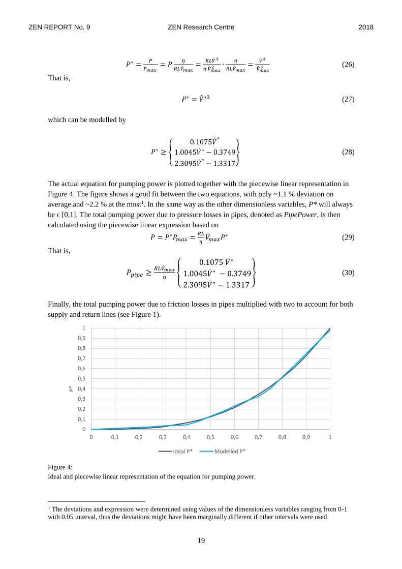
The actual equation for pumping power is plotted together with the piecewise linear representation in

Figure 4. The figure shows a good fit between the two equations, with only ~1.1 % deviation on

average and ~2.2 % at the most1. In the same way as the other dimensionless variables, P* will always

be ϵ [0,1]. The total pumping power due to pressure losses in pipes, denoted as PipePower, is then

calculated using the piecewise linear expression based on

𝑃 = 𝑃∗𝑃𝑚𝑎𝑥 =𝑅𝐿

𝜂�̇�𝑚𝑎𝑥𝑃∗ (29)

That is,

𝑃𝑝𝑖𝑝𝑒 ≥𝑅𝐿�̇�𝑚𝑎𝑥

𝜂{

0.1075 �̇�∗

1.0045�̇�∗ − 0.3749

2.3095�̇�∗ − 1.3317

} (30)

Finally, the total pumping power due to friction losses in pipes multiplied with two to account for both

supply and return lines (see Figure 1).

Figure 4:

Ideal and piecewise linear representation of the equation for pumping power.

1 The deviations and expression were determined using values of the dimensionless variables ranging from 0-1

with 0.05 interval, thus the deviations might have been marginally different if other intervals were used

0

0,1

0,2

0,3

0,4

0,5

0,6

0,7

0,8

0,9

1

0 0,1 0,2 0,3 0,4 0,5 0,6 0,7 0,8 0,9 1

P*

V*Ideal P* Modelled P*


20

The value of maximum flow �̇�𝑚𝑎𝑥, used in calculating the dimensionless variables �̇� , 𝑃∗ and 𝑑𝑝∗, is in

reality dependent on the maximum heat flow and temperature difference in each pipe according to

Equation (1). Obviously, these values are unknown in the model. At present, the default value of the

maximum volume flow in each pipe is calculated using an assumed maximum load for the entire

system:

�̇�𝑚𝑎𝑥 =�̇�𝑚𝑎𝑥

𝑐𝑝(𝑇𝑠𝑢𝑝𝑝𝑙𝑦,𝑚𝑖𝑛−𝑇𝑟𝑒𝑡𝑢𝑟𝑛) (31)

However; even the maximum load for the system is necessarily not known beforehand, and an

approach for defining this should be included in the module. Alternatively; maximum flow in each

pipe in a given network should be defined from a test run, and applied as input to following

simulations. The effect of using different values of �̇�𝑚𝑎𝑥 in calculating �̇�𝑚𝑎𝑥 on the final results is

evaluated in Chapter 4.

Pumping power due to pressure drop at loads

The pumping power at each load is calculated using Equation (8):

𝑃 =𝑑𝑝�̇�

𝜂

where the volume flow at the load is calculated from Equation (1):

�̇� =�̇�𝑙𝑜𝑎𝑑

𝑐𝑝(𝑇𝑖𝑛 − 𝑇𝑜𝑢𝑡)

Here, �̇�𝑙𝑜𝑎𝑑 is known from the �̇�𝑙𝑒𝑠𝑠 variable in the return line after the load, including the heat

demand at the load as well as heat losses in the supply line (see sections 3.1 and 3.2). 𝑇𝑖𝑛 and 𝑇𝑜𝑢𝑡 are

set equal to 𝑇𝑠𝑢𝑝𝑝𝑙𝑦 and 𝑇𝑟𝑒𝑡𝑢𝑟𝑛, respectively, in analogue to Equation (11).

The pressure drop dp is known for the load furthest away – this is the minimum pressure drop the DH

provider is obliged to deliver for their customers, set to 0.7 bar in Trondheim (see section 2.3). For

loads closer to the heat supplier however, the pressure drop will be larger than this (recall Figure 1).

The local pressure drop at loads closer to the supplier is dependent on the local pressure, which is a

variable; hence it cannot directly be used in Equation (8) for calculating the pumping power. For the

sake of simplicity, this extra pressure drop was hence omitted in the present model. The pumping

power due to pressure drop at each load point l, denoted as LoadPower in the model, was thus

calculated from

𝑃𝑙𝑜𝑎𝑑 =𝑑𝑝𝑚𝑖𝑛

𝜂

�̇�𝑙𝑒𝑠𝑠(𝑙,𝑗,𝑟𝑒𝑡𝑢𝑟𝑛)

𝑐𝑝(𝑇𝑠𝑢𝑝𝑝𝑙𝑦−𝑇𝑟𝑒𝑡𝑢𝑟𝑛) (32)

where 𝑑𝑝𝑚𝑖𝑛 is the guaranteed pressure drop at the loads, with a default value of 0.7 bar, and

�̇�𝑙𝑒𝑠𝑠(𝑙, 𝑗, 𝑟𝑒𝑡𝑢𝑟𝑛) is equal to the total heat flow resulting from each load, including both the actual

heat demand and heat losses from pipes leading to the load point as written above.

Omitting the extra pressure drop at load points closer to the heat supplier might result in the total

pumping power being somewhat underestimated. However, the pressure drop due to friction losses in

each pipe – including the pipes leading to each load point – is included in 𝑃𝑝𝑖𝑝𝑒. Thus the model will


21

penalize for extra costs due to pumping power resulting from pressure losses in each pipe line and

each load point, and favour shorter transport distances in choosing the heat source for each load when

multiple heat sources are present.

3.5 The objective function for the DH model

The DH model has the following objective function to be passed to the universal model:

−0.0001 ∑ �̇�𝑑𝑢𝑚𝑝(𝑠, 𝑡)

𝑠,𝑡

+ 𝛾 ∑ �̇�𝑑𝑒𝑓𝑖𝑐𝑖𝑡,1

𝑠,𝑡

(𝑠, 𝑡) + 𝛾 ∑ �̇�𝑑𝑒𝑓𝑖𝑐𝑖𝑡,2

𝑙,𝑡

(𝑙, 𝑡) + 2 𝑐𝑑𝑝 ∑ 𝑃𝑝𝑖𝑝𝑒

(𝑖,𝑗),𝑡

((𝑖, 𝑗), 𝑡)

+ 𝑐𝑑𝑝 ∑ 𝑃𝑙𝑜𝑎𝑑

𝑙,𝑡

(𝑙, 𝑡)

Where the index s is over source points, l over load points, t over time steps, (s,i) over pipes starting

from source points, and (i,j) over all pipes. The objective function has the following terms:

The 1st term is for the heat flow that is dumped, �̇�𝑑𝑢𝑚𝑝,𝑙𝑜𝑎𝑑

The 2nd term is for the heat deficit at sources, �̇�𝑑𝑒𝑓𝑖𝑐𝑖𝑡,1, weighed with penalty γ with a default

value of 100000000

The 3rd term is for the deficit heat at loads, �̇�𝑑𝑒𝑓𝑖𝑐𝑖𝑡,2, weighed with penalty γ

The 4th term is for the pumping power due to pressure losses in pipes, multiplied with the cost

for pressure lift, 𝑙𝑑𝑝 (default 500), and with two to account for both supply and return lines. If

pumping power demand is converted to electric demand, the cost for pressure lift could be

calculated as 𝑙𝑑𝑝 = 𝑐𝑒𝑙/𝜂, where 𝑐𝑒𝑙 is the electricity cost and 𝜂 is the pumping efficiency.

The 5th term is for the total pumping power due to the pressure drop at the loads, 𝑃𝑡𝑜𝑡, multiplied

with the cost for pressure lift.

Thus, the objective of the DH module is to satisfy the demand with minimum heat deficit and

minimum amount of pump work. For the module to cover the heat demand with a given set of heat

supplies, the calculated heat demand, included in the �̇�𝑙𝑒𝑠𝑠 variable in the return line, is passed to the

supply points, p, in the production constraint:

∑ 𝜀𝑠,𝑝�̇�𝑠𝑢𝑝𝑝𝑙𝑦(𝑠, 𝑝, 𝑡)

(𝑠,𝑝)𝑖𝑛 𝑆𝑢𝑝𝑝𝑙𝑦2𝑛𝑒𝑡

+ ∑ 𝜀𝑠,𝑝�̇�𝑛𝑒𝑡2𝑛𝑒𝑡(𝑠, 𝑝, 𝑡)

(𝑠,𝑝)𝑖𝑛 𝑛𝑒𝑡2𝑛𝑒𝑡

− �̇�𝑑𝑢𝑚𝑝,𝑙𝑜𝑎𝑑(𝑝, 𝑡)

+ �̇�𝑑𝑒𝑓𝑖𝑐𝑖𝑡,1(𝑝, 𝑡) = ∑ �̇�𝑙𝑒𝑠𝑠

(𝑝,𝑖)𝑖𝑛 𝑝𝑖𝑝𝑒𝑠

(𝑝, 𝑖, 𝑟𝑒𝑡𝑢𝑟𝑛)

Where

The 1st term on the left hand side is heat flow from the source/supply points to the DH net, with

𝜀𝑠,𝑝 as the connection loss factor

The 2nd term is heat flow from different networks to the DH net, with with 𝜀𝑠,𝑝 as the connection

loss factor

The 3rd term is the dumped heat flow, as defined above. If the heat supply from the given set of

sources exceeds the heat demand, this will result in dumping (rejection) of heat.

The 4th term is the heat deficit at sources. If the given set of heat sources is not able to cover the

heat demand, this results in heat deficit which will be penalized for.

The term on the right hand side is the total heat demand assigned to the source in question.


22

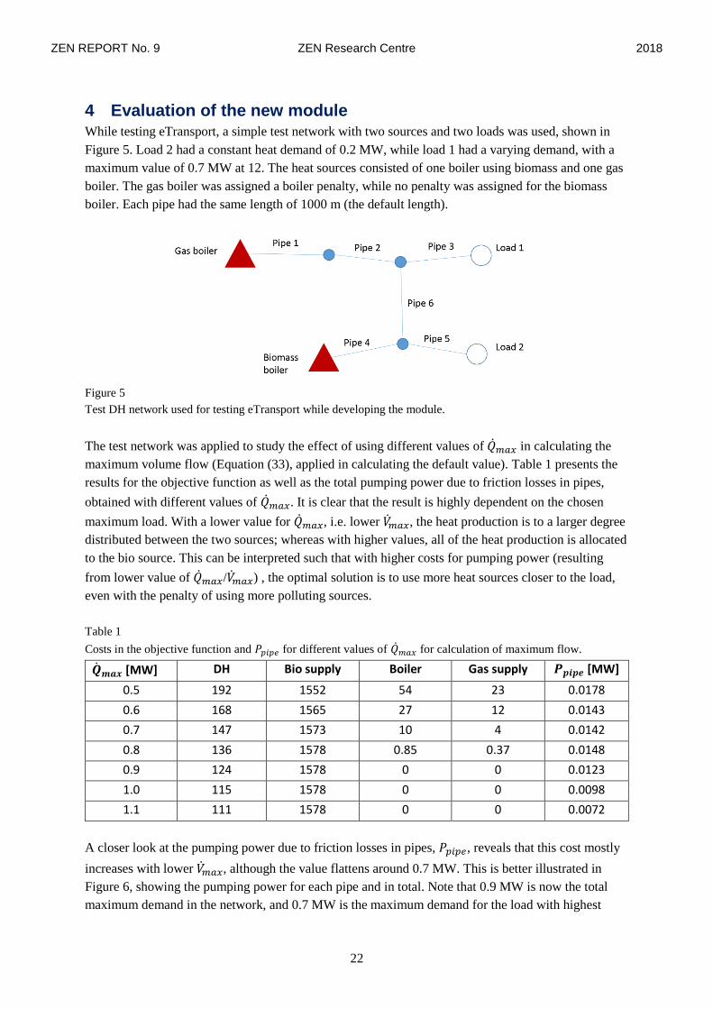
4 Evaluation of the new module While testing eTransport, a simple test network with two sources and two loads was used, shown in

Figure 5. Load 2 had a constant heat demand of 0.2 MW, while load 1 had a varying demand, with a

maximum value of 0.7 MW at 12. The heat sources consisted of one boiler using biomass and one gas

boiler. The gas boiler was assigned a boiler penalty, while no penalty was assigned for the biomass

boiler. Each pipe had the same length of 1000 m (the default length).

Figure 5

Test DH network used for testing eTransport while developing the module.

The test network was applied to study the effect of using different values of �̇�𝑚𝑎𝑥 in calculating the

maximum volume flow (Equation (33), applied in calculating the default value). Table 1 presents the

results for the objective function as well as the total pumping power due to friction losses in pipes,

obtained with different values of �̇�𝑚𝑎𝑥. It is clear that the result is highly dependent on the chosen

maximum load. With a lower value for �̇�𝑚𝑎𝑥, i.e. lower �̇�𝑚𝑎𝑥, the heat production is to a larger degree

distributed between the two sources; whereas with higher values, all of the heat production is allocated

to the bio source. This can be interpreted such that with higher costs for pumping power (resulting

from lower value of �̇�𝑚𝑎𝑥/�̇�𝑚𝑎𝑥) , the optimal solution is to use more heat sources closer to the load,

even with the penalty of using more polluting sources.

Table 1

Costs in the objective function and 𝑃𝑝𝑖𝑝𝑒 for different values of �̇�𝑚𝑎𝑥 for calculation of maximum flow.

�̇�𝒎𝒂𝒙 [MW] DH Bio supply Boiler Gas supply 𝑷𝒑𝒊𝒑𝒆 [MW]

0.5 192 1552 54 23 0.0178

0.6 168 1565 27 12 0.0143

0.7 147 1573 10 4 0.0142

0.8 136 1578 0.85 0.37 0.0148

0.9 124 1578 0 0 0.0123

1.0 115 1578 0 0 0.0098

1.1 111 1578 0 0 0.0072

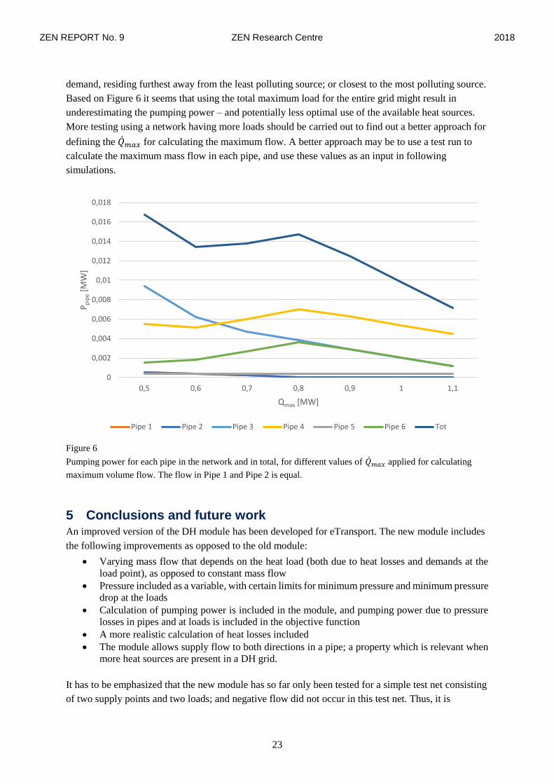
A closer look at the pumping power due to friction losses in pipes, 𝑃𝑝𝑖𝑝𝑒, reveals that this cost mostly

increases with lower �̇�𝑚𝑎𝑥, although the value flattens around 0.7 MW. This is better illustrated in

Figure 6, showing the pumping power for each pipe and in total. Note that 0.9 MW is now the total

maximum demand in the network, and 0.7 MW is the maximum demand for the load with highest


23

demand, residing furthest away from the least polluting source; or closest to the most polluting source.

Based on Figure 6 it seems that using the total maximum load for the entire grid might result in

underestimating the pumping power – and potentially less optimal use of the available heat sources.

More testing using a network having more loads should be carried out to find out a better approach for

defining the �̇�𝑚𝑎𝑥 for calculating the maximum flow. A better approach may be to use a test run to

calculate the maximum mass flow in each pipe, and use these values as an input in following

simulations.

Figure 6

Pumping power for each pipe in the network and in total, for different values of �̇�𝑚𝑎𝑥 applied for calculating

maximum volume flow. The flow in Pipe 1 and Pipe 2 is equal.

5 Conclusions and future work An improved version of the DH module has been developed for eTransport. The new module includes

the following improvements as opposed to the old module:

Varying mass flow that depends on the heat load (both due to heat losses and demands at the

load point), as opposed to constant mass flow

Pressure included as a variable, with certain limits for minimum pressure and minimum pressure

drop at the loads

Calculation of pumping power is included in the module, and pumping power due to pressure

losses in pipes and at loads is included in the objective function

A more realistic calculation of heat losses included

The module allows supply flow to both directions in a pipe; a property which is relevant when

more heat sources are present in a DH grid.

It has to be emphasized that the new module has so far only been tested for a simple test net consisting

of two supply points and two loads; and negative flow did not occur in this test net. Thus, it is

0

0,002

0,004

0,006

0,008

0,01

0,012

0,014

0,016

0,018

0,5 0,6 0,7 0,8 0,9 1 1,1

Pp

ipe

[MW

]

Qmax [MW]

Pipe 1 Pipe 2 Pipe 3 Pipe 4 Pipe 5 Pipe 6 Tot


24

important that the module is tested for more complex systems. It is possible and even probable that

there will be a need for improvements later on.

The new module has also a few limitations, to be regarded as suggestions for future work:

1. The value of maximum mass flow, applied for calculating pressure drops and pumping power

due to friction losses in the pipes, is currently constant in each pipe. Its default value is calculated

using a hypothetical value for maximum demand in the grid. A more sophisticated approach,

potentially considering the maximum demand of the load furthest away, or the maximum

demand of a single load in the network, should be applied, as discussed in section 4. A better

approach may be to carry out a test simulation to calculate the maximum mass flow in each

pipe, and use these values as an input in following simulations.

2. At present, both the supply and return temperatures are constant, with same values at each load

and time step. In conventional high-temperature DH systems the supply temperature is a

function of the outdoor temperature. In low-temperature systems, likely to become common in

the future, the supply temperature may be kept constant throughout the year. eTransport will

probably be applied to simulate both high- and low-temperature systems, and outdoor

temperature compensation of the supply temperature should thus be included in the module. To

be able to do this, the outdoor temperature at each time step as well as the desired maximum

and minimum supply temperature limits should be included as input parameters.

Return temperature is a function of the inlet temperature, and depends also strongly on the

heat exchange conditions at the loads. Dependency on the inlet temperature could be

implemented simply with a constant temperature drop over a load. A more realistic approach

would be to model heat exchange at the loads, which would increase the model complexity

significantly. We hence suggest to implement the simple approach for calculating the return

temperature: a constant temperature drop over a load.

3. The pumping power demand is presently included in the objective function of the DH module,

however it could be made a demand input for electricity. In this case a conversion unit is

required.

4. The original version of the DH module had some parameters that were omitted in the present

version, but which may be useful to re-introduce:

a. Time_Delay parameter, a delay for the water flowing from one end of a pipe to the other

by a given number of time steps. This parameter should be included if it is desirable to

include the thermal storage capacity of the network in the model.

b. The temperature requirement at loads, set DH_Load_req. The developer did not manage

this, and a new requirement for minimum temperature at loads, equal for all loads and

time steps, was introduced instead. This new parameter could however be made time-

dependent and different for different loads, if desirable. In real systems, the minimum

supply temperature at loads may be dependent on the ambient temperature, and different

types of customers (e.g. apartment buildings vs. commercial buildings) may also have

different temperature demands.

5. The extra pressure loss at loads closer to the heat supply was omitted, as discussed in section

3.4. This may lead into underestimation of the pumping power. An approach to include these

losses should be developed, if this shortcoming is regarded considerable.

6. The module should have a way to set heat losses to zero if mass flow is zero, as discussed in

section 3.2. Currently there is no such constraint.


25

References

Dalla Rosa, A. L. (2011). Method for optimal design of pipes for low-energy district heating, with focus

on heat losses. Energy, 2407-2418.

Fourer, R. G. (2003). AMPL: A Modeling Language for Mathematical Programming. Thomson.

Fredriksen, S.;& Werner, S. (2014). District heating and cooling. Studentlitteratur AB.

Kauko, H. K. (2018). Dynamic modeling of local district heating grids with prosumers: A case study for

Norway. Energy, 261-271.

Wallentèn, P. (1991). Steady-state heat loss from insulated pipes. LTH, Lunds Tekniska Högskola.


26

A1. Appendix 1: Parameters, variables and sets

Type Name Definition Default Restrictions Explanation

# Junction points and set of all points

set DH_Junction_points

{}

Set containing junction points

set DH_Points := DH_Load_points union

DH_Production_points

union

DH_Junction_points

Set containing all points; load,

junction and source/production

points

set DH_Directions := {"DH_OUT",

"DH_BACK"};

Supply and return denoted by out

and back: Out is water from the

heater to the load. Back is the

return water.

set DH_Ends := { "DH_THIS", "DH_FAR"

};

Ends of pipes, denoted by this and

far. This is the end listet first in the

ordered pair defining a pipeline, FAR

is the end listed last. The end closest

to the source should be listed first.

set DH_Pipe_lines within { DH_Points,

DH_Points }

Set of all DH pipelines

param DH_Water_flow DH_Water_flow{

DH_Pipe_lines }

1

Old water flow, kept constant, not in

use but cannot be removed without

error message (the program uses it

from outside the model).

param DH_Time_delay DH_Time_delay{DH_Pipe_

lines} integer

0

Transportation time in pipes,

currently not in use (how many time

steps water entering a pipe is

delayed before reaching exit)

param DH_max_delay :=max{(i,j) in

DH_Pipe_lines}

DH_Time_delay[i,j]

The longest transportation time in

the pipe lines

#Energy parameters

param DH_Water_heating_fa

ctor

4.2

Total water flow multiplied by

specific heat ( given in

MWh/(h*(m3/s)*K)): mdot*c_p

param Users_heat_loss_facto

r

Users_heat_loss_factor{D

H_Pipe_lines}

10

Heat loss factor for pipe lines

defined by the user, in [W/m]

param DH_Heat_loss_factor DH_Heat_loss_factor{(i,j)

in DH_Pipe_lines}

Users_heat_loss_fac

tor[i,j]/40000000;

Heat loss factor in correct units:

MW/m divided by temp. difference

at test conditions for pipes (50 °C in

pipe and assumed 10 °C for

ambient). New unit is then

[MW/(mK)]

param DH_max_demand DH_max_demand 0.7

Dimensioning load, applied for

calculating the default value for

maximum flow in the grid.

#Heat loss and delivered load

var Qless Qless{(i,j) in

DH_Pipe_lines, d in

DH_Directions, e in

Variable equal to the heat removed

from the water after it left the heat

central.


27


DH_Ends, t in

Time_steps};

#Temperature parameters

param DH_max_temp DH_max_temp{ (i,j) in

DH_Pipe_lines, d in

DH_Directions }

120

Requirement for max DH

temperature

param DH_min_temp DH_min_temp{ (i,j) in

DH_Pipe_lines, d in

DH_Directions }

15

Requirement for min DH

temperature

param T_supply

65

param T_min_supply

63

Minimum temperature requirement

at loads.

set DH_Load_req

{}

Load-dependent minimum

temperature reqiurement. Currently

unused

param DH_water_temp DH_water_temp{(i,j) in

DH_Pipe_lines, d in

DH_directions, e in

DH_Ends, t in Time_steps}

1

Currently unused, but the program

uses it from outside and an error

message occurs if removed

set DH_All_time_steps := -DH_max_delay+1 ..

n_time_step

Old variable for some unknown

purpose, not deleted

#Pressure parameters and variables (new from the previous

model)

param DH_min_pressure = 0.1

Minimum pressure in [MPa]

param DH_max_pressure = 0.5

Max pressure in [Mpa]. Max p is

actually 10 bar, however as only

return pressure is calculated, it is set

to 5 bar = 0.5 Mpa

var DH_pressure DH_pressure { (i,j) in

DH_Pipe_lines, e in

DH_Ends, t in Time_steps }

>=

DH_min_pressure

<=

DH_max_pressure

-0.035;

Pressure in return line in [MPa]

param cost_dp

500

To be deleted if power demand is

converted to electric demand. In this

case cost_dp= c_el/efficiency =500

kr/MWh *0.5^(-1)=1000

[kr/(MPa∙m^3/s∙h)]

var dp dp { (i,j) in DH_Pipe_lines,

t in Time_steps}

>=0 Pressure drop in pipes

var dpN dpN { (i,j) in

DH_Pipe_lines, t in

Time_steps}

<=0 Pressure drop in pipes for negative

water flow.

param dp_DH_Load

0.07

Guaranteed pressure drop across a

load, set to 0.7 bar=0.07 MPa=70

kPa

param Rvalue

150

Max allowed pressure drop per

metre pipe at a given max water

flow, set to 150 Pa/m

param DH_Pipe_Length DH_Pipe_Length {

DH_Pipe_lines }

1000

Pipe length in m


28


param max_water_flow max_water_flow {(i,j) in

DH_Pipe_lines}

DH_max_demand/(

DH_Water_heating_

factor*(T_min_suppl

y-DH_min_temp[i,j,

"DH_BACK"]))

Max flow in each pipe [m3/s]. The

default value calculated from

DH_max_demand/(DH_Water_heati

ng_factor*(T_min_supply-

DH_min_temp[i,j, "DH_BACK"]))

#Water flow

var DH_Waterflow DH_Waterflow{ (i,j) in

DH_Pipe_lines, t in

Time_steps }

>=0 Variable for positive flow in pipes

var DH_WaterflowN DH_WaterflowN{ (i,j) in

DH_Pipe_lines, t in

Time_steps }

<=0 Variable for water flow in opposite

direction.

#Pumping power

param pumpEff

0.5

Pump efficiency with a default value

of 50%

var PipePower PipePower{(i,j) in

DH_Pipe_lines, t in

Time_steps};

Pumping power due to friction

losses in pipes

var LoadPower LoadPower{l in

DH_Load_points, t in

Time_steps};

Pumping power due to throttling

losses at loads

# within Load_points (part of older code)

param DH_Input_temp_req DH_Input_temp_req{

DH_Load_req };

Requirement for supply

temperature at each load, currently

not in use.

param DH_deficit_penalty

100000000

Penalty for not covering demands

set DH_Const_time_steps := {};

It is possible to insist that the

outgoing temperature shall be fixed.

Const_time_steps define a set of

time steps for which the outgoing

temperature should be the same

# Dump load

var DH_dump_load DH_dump_load{

DH_Production_points,

Time_steps }

>=0 Amount of heat flow dumped at

production points

var DH_deficit1 DH_deficit1{

DH_Production_points,Ti

me_steps }

>=0 Amount of insufficient heat flow at

sources.

var DH_deficit2 DH_deficit2{

DH_Load_points,Time_ste

ps }

>=0 Amount of insufficient heat flow at

loads, currently not calculated


29

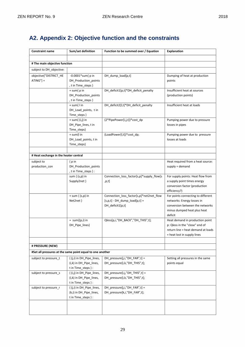
A2. Appendix 2: Objective function and the constraints

Constraint name Sum/set definition Function to be summed over / Equation Explanation

# The main objective function

subject to DH_objective:

objective["DISTRICT_HE

ATING"] =

-0.0001*sum{ p in


, t in Time_steps }

DH_dump_load[p,t] Dumping of heat at production

points

+ sum{ p in


, t in Time_steps }

DH_deficit1[p,t]*DH_deficit_penalty Insufficient heat at sources

(production points)

+ sum{ l in


Time_steps }

DH_deficit2[l,t]*DH_deficit_penalty Insufficient heat at loads

+ sum{ (i,j) in

DH_Pipe_lines, t in

Time_steps}

(2*PipePower[i,j,t])*cost_dp Pumping power due to pressure

losses in pipes

+ sum{l in


Time_steps}

(LoadPower[l,t])*cost_dp; Pumping power due to pressure

losses at loads

# Heat exchange in the heater central

subject to

production_con

{ p in


, t in Time_steps } :

Heat required from a heat source:

supply = demand

sum { (s,p) in

Supply2net }

Connection_loss_factor[s,p]*supply_flow[s

,p,t]

For supply points: Heat flow from

a supply point times energy

conversion factor (production

efficiency?)

+ sum { (s,p) in

Net2net }

Connection_loss_factor[s,p]*net2net_flow

[s,p,t] - DH_dump_load[p,t] +

DH_deficit1[p,t]

For points connecting to different

networks: Energy losses in

conversion between the networks

minus dumped heat plus heat

deficit

= sum{(p,i) in

DH_Pipe_lines}

Qless[p,i,"DH_BACK","DH_THIS",t]; Heat demand in production point

p: Qless in the "close" end of

return line = heat demand at loads

+ heat lost in supply lines

# PRESSURE (NEW)

#Set all pressures at the same point equal to one another

subject to pressure_t { (j,i) in DH_Pipe_lines,

(i,k) in DH_Pipe_lines,

t in Time_steps } :

DH_pressure[j,i,"DH_FAR",t] =

DH_pressure[i,k,"DH_THIS",t];

Setting all pressures in the same

points equal

subject to pressure_s { (i,j) in DH_Pipe_lines,

(i,k) in DH_Pipe_lines,

t in Time_steps } :

DH_pressure[i,j,"DH_THIS",t] =

DH_pressure[i,k,"DH_THIS",t];

subject to pressure_r { (j,i) in DH_Pipe_lines,

(k,i) in DH_Pipe_lines,

t in Time_steps } :

DH_pressure[j,i,"DH_FAR",t] =

DH_pressure[k,i,"DH_FAR",t];


30


#The lowest pressure in the system should always be DH_min_pressure

subject to

pressure_minimum

{s in


, t in Time_steps } :

min{(s,j) in

DH_Pipe_lines}(DH_pressure[s,j,"DH_THIS"

,t]) = DH_min_pressure;

Setting pressure in source points

equal to minimum pressure (1 bar)

#Calculating pressure losses, for positive water flows, that is, DH_Waterflow>0

subject to find_dp1 { i in DH_Points, (j,i) in

DH_Pipe_lines, t in

Time_steps }:

dp[j,i,t]>=Rvalue*10^(-

6)*DH_Pipe_Length[j,i]*

0.24*DH_Waterflow[j,i,t]

/max_water_flow[j,i];

Calculation of the pressure drop

using a piecewise linear equation

for dp


DH_Pipe_lines, t in

Time_steps }:


6)*DH_Pipe_Length[j,i]*(-

0.24+1*DH_Waterflow[j,i,t]/max_water_fl

ow[j,i]);


DH_Pipe_lines, t in

Time_steps }:



0.71+1.7*DH_Waterflow[j,i,t]/max_water_

flow[j,i]);


DH_Pipe_lines, t in

Time_steps }:

dpN[j,i,t]<=Rvalue*10^(-


0.24*DH_WaterflowN[j,i,t]

/max_water_flow[j,i];

Same eqations for negative flow


DH_Pipe_lines, t in

Time_steps }:



0.24+1*DH_WaterflowN[j,i,t]/max_water_

flow[j,i]);


DH_Pipe_lines, t in

Time_steps }:



0.71+1.7*DH_WaterflowN[j,i,t]/max_water

_flow[j,i]);

subject to NoFlowNodp { i in DH_Points, (j,i) in

DH_Pipe_lines, t in

Time_steps }:

dp[j,i,t]<=Rvalue*10^(-


(DH_Waterflow[j,i,t]/max_water_flow[j,i]);

Preventing positive and negative

flows at the same time.

subject to

NoFlowNodpN

{ i in DH_Points, (j,i) in

DH_Pipe_lines, t in

Time_steps }:

dpN[j,i,t]>=Rvalue*10^(-


(DH_WaterflowN[j,i,t]/max_water_flow[j,i]

);

Same for negative flow.

subject to pressure_loss { (j,i) in DH_Pipe_lines,

t in Time_steps } :

DH_pressure[j,i,"DH_THIS",t] +dp[j,i,t]

=DH_pressure[j,i,"DH_FAR", t];

Adding the calculated pressure

losses in the return pipe in the

case when only positive flow is

considered. Due to symmetry,

only the return is calculated.

subject to pressure_loss { (j,i) in DH_Pipe_lines,

t in Time_steps } :

DH_pressure[j,i,"DH_THIS",t] +dp[j,i,t]

=DH_pressure[j,i,"DH_FAR", t]-dpN[j,i,t];

Same for the case when negative

flow is included.

#MASS FLOW

subject to water_flow { p in

DH_Junction_points, t

in Time_steps}:

sum{ (l,p) in DH_Pipe_lines}

(DH_Waterflow[l,p,t]) = sum{(p,j) in

DH_Pipe_lines} (DH_Waterflow[p,j,t]);

Mass balance equation for all

points

subject to water_flow { p in


in Time_steps}:

sum{ (l,p) in DH_Pipe_lines}

(DH_Waterflow[l,p,t]+DH_WaterflowN[l,p,

t])= sum{(p,j) in DH_Pipe_lines}

(DH_Waterflow[p,j,t]+DH_WaterflowN[p,j,

t]);

Mass balance equation for the

two-way model. Works only if

everything is coupled to junctions.


31


subject to

NoExtraWaterFlowLoad{

{l in DH_Load_points,

(i,l) in DH_Pipe_lines, t

in Time_steps}:

DH_WaterflowN[i,l,t]=0; Ensuring that there is no negative

flow at loads

subject to

NoExtraWaterFlowSourc

e

{s in


, (s,i) in

DH_Pipe_lines, t in

Time_steps}:

DH_WaterflowN[s,i,t]=0; Ensuring that there is no negative

flow at sources

#MASS, HEAT AND TEMPERATURE DEMANDS

subject to

TempRequirement

{l in DH_Load_points,


in Time_steps}:

Qless[i,l,"DH_OUT","DH_FAR",t]<=DH_Wat

er_heating_factor* (T_supply-

T_min_supply)*DH_Waterflow[i,l,t];

Sets the temperature drop within

pipes due to heat loss to be within

allowed range. Not in use at

present.

subject to TempMass {l in DH_Load_points,

(i,l) in DH_Pipe_lines,

(l,j) in Net2load, t in

Time_steps}:

Qless[i,l,"DH_OUT","DH_FAR",t]+load_flow

[l,j,t]

<=DH_Water_heating_factor*(T_supply-

DH_min_temp[i,l,"DH_BACK"])

*DH_Waterflow[i,l,t];

Demand that the water flow

covers the demand in a realistic

temp range

subject to

TempMassSource

{p in


, (p,i) in

DH_Pipe_lines, t in

Time_steps}:

DH_Waterflow[p,i,t] <=

Qless[p,i,"DH_BACK","DH_THIS",t]/DH_Wa

ter_heating_factor;

For sources: ensures that

waterflow is zero if there is no

heat flow from the source; and

that heat flow is nonzero if

waterflow is nonzero.

#HEAT FLOW

subject to HeatCentral {s in


, t in Time_steps, (s,i)

in DH_Pipe_lines}:

Qless[s,i,"DH_OUT","DH_THIS",t]>=0; Requiring that lost heat is always

lost - for pipes out of production

points. Shall be equal to 0, but

better to allow inequality to avoid

errors.

subject to

HeatLossIsLoss

{t in Time_steps, l in

DH_Load_points, (i,l)

in DH_Pipe_lines}:

Qless[i,l,"DH_OUT","DH_THIS",t]>=0; Same for supply lines going in to

loads. Without this requirement,

the lost heat may be heat input to

the system.

subject to

HeatLossFromLoad

{t in Time_steps, l in

DH_Load_points, (i,l)

in DH_Pipe_lines}:

Qless[i,l,"DH_BACK","DH_FAR",t]>=0; Same for return lines going out

from a load.

subject to

HeatLossIsLossJunction

{t in Time_steps, j in

DH_Junction_points,

(j,i) in DH_Pipe_lines}:

Qless[j,i,"DH_OUT","DH_THIS",t]>=0; The same requirement for supply

lines going to junction points.

subject to PipeLosses {(i,j) in DH_Pipe_lines,

t in Time_steps}:

Qless[i,j,"DH_OUT","DH_FAR",t]=

Qless[i,j,"DH_OUT","DH_THIS",t]+DH_Pipe

_Length[i,j]*(T_supply-

Outdoor_temp[t])*DH_Heat_loss_factor[i,j

];

Calculating the heat losses and

adding them to the far end of the

supply lines. Uncertain if this will

work for negative flow

subject to NoPipeLosses {(i,j) in DH_Pipe_lines,

t in Time_steps}:

Qless[i,j,"DH_BACK","DH_FAR",t]=Qless[i,j,

"DH_BACK","DH_THIS",t];

Requirement that there are no

losses in the return line (realistic

approximation).

subject to

EnergyBalanceOut

{p in


in Time_steps}:

sum{(i,p) in DH_Pipe_lines} Qless[i,p,

d,"DH_OUT","DH_FAR",t]= sum{(p,j) in

DH_Pipe_lines}

Qless[p,j,d,"DH_OUT","DH_THIS",t];

Energy balance equation for the

junction points for supply lines


32


subject to

EnergyBalanceBack

{p in


in Time_steps}:

sum{(i,p) in DH_Pipe_lines} Qless[i,p,

d,"DH_BACK","DH_FAR",t]= sum{(p,j) in

DH_Pipe_lines}

Qless[p,j,d,"DH_BACK","DH_THIS",t];

Energy balance equation for the

junction points for return lines

subject to LoadHeat {l in DH_Load_points,

t in Time_steps}:

sum{(i,l) in DH_Pipe_lines}

Qless[i,l,"DH_OUT","DH_FAR",t]+ sum {

(l,p) in Net2load } load_flow[l,p,t]

=sum{(i,l) in DH_Pipe_lines}

Qless[i,l,"DH_BACK","DH_FAR",t];

Taking out heat at load=Adding

heat loads to the Qless-variable in

the return line

#POWER

#Calculation of the pumping power due to pressure losses in pipes using a piecewise linear equation

subject to

dpPowerPipe1

{(i,j) in DH_Pipe_lines,

t in Time_steps}:

PipePower[i,j,t]*pumpEff>=0.1075*(DH_W

aterflow[i,j,t]-

DH_WaterflowN[i,j,t])/max_water_flow[i,j]

* Rvalue*10^(-6)

*DH_Pipe_Length[i,j]*max_water_flow[i,j];

Calculation for the required

pumping power due to friction

losses in pipes.

subject to

dpPowerPipe2


t in Time_steps}:

PipePower[i,j,t]*pumpEff>=(-

0.3749+1.0044*(DH_Waterflow[i,j,t]-


) *Rvalue*10^(-6)


subject to

dpPowerPipe3


t in Time_steps}:

PipePower[i,j,t]*pumpEff>=(-

1.3317+2.3095*(DH_Waterflow[i,j,t]-


)* Rvalue*10^(-6)


#Calculate required power for pumping due to throttling losses at loads

subject to dpPowerLoad { l in DH_Load_points,


in Time_steps}:

LoadPower[l,t]*pumpEff=dp_DH_Load*Qle

ss[i,l,"DH_BACK", "DH_FAR",t]/(T_supply-

DH_min_temp[i,l,"DH_BACK"])/

DH_Water_heating_factor;


33


34


35

linear optimization of district heating systems · oppgraderte modulen er mer realistisk i forhold...

Documents