linear programming - universidad tecnológica de panamá · linear programming is a response to...

H. R. Alvarez A., Ph. D. 1

Linear Programming


Introduction

It is a mathematical technique that allows the selection of the best course of action defining a program of feasible actions.

The objective of LP is to assign resources that are scarce to different activities competing for them.

The model that describes the different relationships among variables is composed of linear functions.

George Dantzig is considered the father of LP


General formulation

The main statement of the problem can be as follows:

To optimize a dependent variable, expressed as linear function of n independent variables, subject to a series of constraints that are also linear function of the n independent variables.


The dependent variable is known as the Objective Function.

This function is related to economic concepts such as earnings, income, time, cost, distance, etc.

The independent variables are known as decision variables.

General formulation


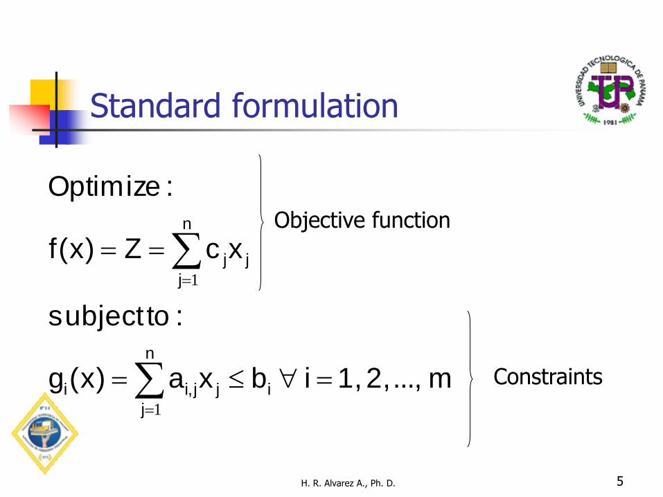
Standard formulation

m ..., 2, 1,i bxa)x(g

:to subject

xcZ)x(f

:Optimize

ij

n

j

j,ii

n

j

jj

1

1

Objective function

Constraints


Given that:

f(.): objective function

xj : decision variables

cj : coefficient of the jth decision variable in the objective function, for j = 1,…, n

a1,j: coefficient of the jth decision variable in the ith restriction, for i = 1,…, m

bi : constant or boundary of the ith constraint.


The constraints:

Linear programming is a response to situations that require the maximization or minimization of certain functions which are subject to limitations. These limitations are called constraints.

There are three types of constraints:

g(x) ≤ b

g(x) ≥ b, or

g(x) = b

Constraints type ≤ ensure that the use of resources do not exceed certain amount of it.

Constraints type ≥ ensure that the use of certain resources will satisfy a minimum amount of it.

Constraints type = ensure that the use of certain resource will be exactly as defined.


Model formulation: steps

Good understanding of the problem

Identify decision variables

Define the objective function

Define constraints

Identify lower and upper boundaries of the decision variables

One example from Hillier: The Wyndor Case

A window factory produces high quality glass products including doors and window panels.

The factory has three plants. Frames are assembled in Plant A, wood elements are produced in Plant B, and cutting of glass panels and final assembly are done in Plant C.


Example…

Management has decided to increase production through two additional products: a special type of door and a safety window.

They consider that there is enough capacity to produce both products without sacrificing the current production, although they might have to compete with the exceeding capacity in Plant C.

Additionally, no inventories will be allowed, that is, all production will be sold.



Problem Information

Plant

Resources used by unit

Availability of resources Product

Doors Windows

A 1 0 4

B 0 2 12

C 3 2 18

Earnings per unit

3 5


Example…

The organization is interested in determining the optimal product mix of doors and windows in order to maximize total earnings.


Formulation

What is the objective? To find how many doors and windows should

produce to maximize income.

Which are the decision variables? The amount of doors (x1) and windows (x2) to be

produced

What is the objective function? Total earnings

What are the constraints? Plant capacities


Standard formulation

Maximize:

Z= 3x1 + 5x2

Subject to:

x1 ≤ 4 2x2 ≤ 12 3x1 + 2x2 ≤ 18 x1, x2 ≥ 0


Solving the problem

By intuition

Complete enumeration

Graphic solution

Exact mathematical methods

Simplex

Other approaches

Heuristics


The Graphical Solution

A LP problem can be represented as a convex region.

The feasible region is formed by the set of values of the decision variable that simultaneously satisfy all the constraints

It is a convex region, so that, all the corners are a weighted combination of the points forming the feasible region.

Candidate solutions for global optima are located in the intersections of the constraints that form the different corners of the convex region.


The optimal solution

Thus, an optimal solution is located in a corner.

There is a finite number of corner points.

If a corner point provides a solution equal or better than any of the adjacent neighbors, then it is optima.

The Graphical Solution of Wyndor

x2

x1

(0,6)

(4,0)

(4,3)

(2,6)

Feasible region

Objective function

Corners x1 x2

x1 x2 3 5

0 6 30

2 6 36

4 3 27

4 0 12

Optima

The optimal solution

Meaning of the solution

The optimal production mix is:

2 doors and 6 safety windows

A total income of 36 monetary units

In Plant A there would be 2 units of resources available

No available resources in both Plant B and C ;(2*6 = 12 and 3*2 + 2*6 = 18)

Example


•

• Find the maximal and minimal value of

z = 3x + 4y subject to the following constraints,

for x, and y unrestricted:


(2, 6)

(6, 4)

(-1, -3)

Example 2

A school is preparing a trip for 400 students. The company who is providing the transportation has 10 buses of 50 seats each and 8 buses of 40 seats, but only has 9 drivers available. The rental cost for a large bus is $800 and $600 for the small bus. Calculate how many buses of each type should be used for the trip for the least possible cost.


Example 3 Two Crude Petroleum runs a small refinery on the Texas coast. The refinery distills crude petroleum from two sources, Saudi Arabia and Venezuela, into three main products: gasoline, jet fuel, and lubricants.

The crudes differ in chemical composition and thus yield different product mixes. Each barrel of Saudi crude yields 0.3 barrel of gasoline, 0.4 barrel of jet fuel, and 0.2 barrel of lubricants. On the other hand, each barrel of Venezuelan crude yields 0.4 barrel of gasoline, but only 0.2 barrel of jet fuel and 0.3 barrel of lubricants. The remaining 10% of each barrel is lost to refining.

The crudes also differ in cost and availability. Two Crude can purchase up to 9,000 barrels per day from Saudi Arabia at $68 per barrel. Up to 6,000 per day of Venezuelan petroleum are also available at the lower cost of $61 per barrel because of the transportation costs.

Two Crudes contracts with independent distributors require to produce 2,000 barrels per day of gasoline, 1500 barrels per day of jet fuel, and 500 barrels per day of lubricants. How can these requirements can be fulfilled most efficiently?

Example 4

A transport company has two types of trucks, Type A and Type B. Type A has a refrigerated capacity of 20 m3 and a non-refrigerated capacity of 40 m3 while Type B has the same overall volume with equal sections for refrigerated and non-refrigerated stock. A grocer needs to hire trucks for the transport of at least 3,000 m3 of refrigerated stock and 4 000 m3 of non-refrigerated stock. The cost per kilometer of a Type A is $30, and $40 for Type B. How many trucks of each type should the grocer rent to achieve the minimum total cost?


Example 5

A company makes two products (X and Y) using two machines (A and

B). Each unit of X that is produced requires 50 minutes processing time

on machine A and 30 minutes processing time on machine B. Each unit

of Y that is produced requires 24 minutes processing time on machine

A and 33 minutes processing time on machine B.

At the start of the current week there are 30 units of X and 90 units of Y

in stock. Available processing time on machine A is forecast to be 40

hours and on machine B is forecast to be 35 hours.

The demand for X in the current week is forecast to be 75 units and for

Y is forecast to be 95 units. Company policy is to maximise the

combined sum of the units of X and the units of Y in stock at the end of

the week.

Formulate the problem of deciding how much of each product to make

in the current week as a linear program.


Some special considerations

Alternate solutions: If there are more than one solution, at least two of them are adjacent.


Unbounded solution: the region of possible solutions is not bounded by a constraint, thus the solution has infinite possibilities. Normally this situation is due to a formulation error.


Unfeasible solution: when a set of solutions is an empty set, there are no possible points that satisfy all the constraints.

Region for constraints 1 and 2

Region for constraint 3


Redundant constraints: When there are constraints that do not affect the feasible region, they are redundant in the solution and do not affect it.

Redundant constraints


The Simplex Method

Developed in 1947 by George Dantzig as part of a project for the DoD

Is based on the corner solution property of L. P.

O(n) complexity


The Simplex Method …

It is an iterative process Takes advantage of the concept of the

corner point.

The initial solution requires a standard or augmented formulation.

It searches for a solution in all the corner points in n, beginning at the origin of the convex region.

It has an optimality test.

General description Assume a standard LP formulation:

Such that:

In the canonical form


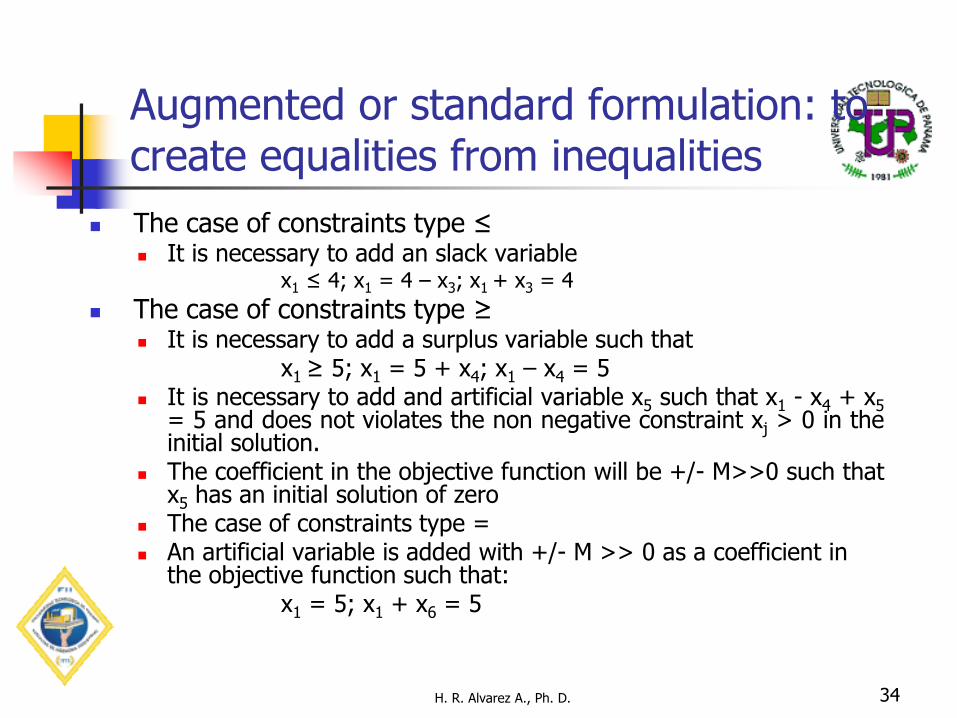
Augmented or standard formulation: to create equalities from inequalities

The case of constraints type ≤ It is necessary to add an slack variable

x1 ≤ 4; x1 = 4 – x3; x1 + x3 = 4

The case of constraints type ≥ It is necessary to add a surplus variable such that x1 ≥ 5; x1 = 5 + x4; x1 – x4 = 5 It is necessary to add and artificial variable x5 such that x1 - x4 + x5

= 5 and does not violates the non negative constraint xj > 0 in the initial solution.

The coefficient in the objective function will be +/- M>>0 such that x5 has an initial solution of zero

The case of constraints type = An artificial variable is added with +/- M >> 0 as a coefficient in

the objective function such that: x1 = 5; x1 + x6 = 5


The initial solution

Simplex assumes an initial solution at the origin, thus all the initial variables are set in zero.

Since this condition violates the main constraints in the formulation, Simplex needs to generate an augmented formulation.


The augmented solution

It is the solution of a linear programming problem originally formulated in the standard manner

It is an augmented corner point solution

A basic feasible solution is a feasible augmented corner point solution


Properties of a solution

Degrees of freedom: it is the difference between the number of variables, including the slack, surplus or artificial variables and the number of constraints, not including the nonnegative.

To solve the system it is necessary to assume arbitrary values, zero in this case.

The variables that are set to zero are known as non basic variables.

The variables included in the solution are known as basic variables.


The standard formulation:

The initial tableau

Slack variables

At the initial solution the decision variables x1,…, xn = 0, and are non basic variables in the solution

The set of variables in the solution are called basic variables, and the solution a basic feasible solution


The iterative process

In order to find a better adjacent solution, basic variable will become non basic and a non basic will enter the solution as a basic.

The entering variable will be the one that improves the objective solution faster.

The leaving variable will be the first one to become zero.

The optimal solution is found when there are no more improving non basic variables.

Moving within the n space

Let the set of basic variables, such that in the initial solution = {xn+i}i=1, m

Let be the set of non basic variables, such that in the initial solution ={xi}i=1,n

To replace xr by xs the ars element is called the pivot point and the operation becomes a Gaussian elimination such that:

Moving within the n space

The entering xs will be selected according to an optimality test, i. e., the most positive or negative variable.

One strategy would be to select whichever variable has the greatest reduced cost . In linear programming, reduced cost, or opportunity cost, is the amount by which an objective function coefficient would have to improve (so increase for maximization problem, decrease for minimization problem) before it would be possible for a corresponding variable to assume a positive value in the optimal solution.

The leaving xr must be selected as the basic variable corresponding to the smallest positive ration of the values of the current right hand side of the current positive constraint coefficient of the entering non-basic variable xs


The Wyndor case: the standard formulation

Minimize Z such that:

Z – 3x1 – 5x2 = 0

s.t.

x1 + x3 = 4

2x2 +x4 = 12

3x1 + 2x2 + x5 = 18

There are to decision variables and three slack variables. In addition there are three constraints. Thus, the degree of freedom is two.



The basic initial solution will be:

x1 = x2 = 0 and

x3 = 4

x4 = 12

x5 = 18

Since this solution is not an optima, the iteration process begins.

The Wyndor case: the standard formulation – initial tableau

X1 x2 x3 x4 x5 b

x3 1 0 1 0 0 4

x4 0 2 0 1 0 12

X5 3 2 0 0 1 18

z -3 -5 0 0 0 0

18/2

12/2

4/0

Enters

Leaves

Formulation and solution of the Wyndor Example with AMPL



Formulation and Solution of the sign unrestricted example

The Duality Every linear programming problem, referred to as a primal

problem, can be converted into a dual problem, which provides an upper bound to the optimal value of the primal problem

The primary problem and the dual problem are complementary. A solution to either one determines a solution to both.

In the primal problem, the objective function is a linear combination of n variables. There are m constraints, each of which places an upper bound on a linear combination of the n variables. The goal is to maximize the value of the objective function subject to the constraints. A solution is a vector (a list) of n values that achieves the maximum value for the objective function.

In the dual problem, the objective function is a linear combination of the m values that are the limits in the m constraints from the primal problem. There are n dual constraints, each of which places a lower bound on a linear combination of m dual variables.


The Dual

Every maximization (minimization) problem in L. P. has an equivalent dual minimization (maximization) problem.

0

j

n

1j

ijji,

n

1j

jj

x

m ..., 2, 1,i bxa

:t. .s

xcZ Max

imalPr

0

1

i

m

i

ij,i

m

1i

ii

y

n ..., 2, 1, j cjya

:.t .s

yb Y Min

:Dual


Relationship Primal - Dual

Primal problem

Dual

Problem

Coefficients of

yi

Coefficients of

x1 x2 … xn ≤ bi

Coefficients of the Objective

function

(Minimize)

Y1 a1,1 a1,2 … a1,n b1

y2 a2,1 a2,2 … a2,n b2

.

.

.

.

.

.

.

.

.

ym am,1 am,2 … am,n bm

≥ cj c1 c2 … cn

Primal solution

Dual solution


The solution of the dual

The solution of {yj}ji=1,m represents the contribution of the unit profit of resource j when the primal is solved.

The shadow price is the change in the objective value of the optimal solution of an optimization problem obtained by relaxing the constraint by one unit – it is the marginal utility of relaxing the constraint, or equivalently the marginal cost of strengthening the constraint.

Thus the solution of the dual defines the shadow prices of the resources.

Post-optimal or sensitivity analysis

It is one of the most important steps in LP

It consists of determining how sensible is the model’s optimal solution if certain parameters such as the Objective Function coefficients ot the independent terms of the los coeficientes deconstraints change.



Post-optimal or Sensitivity analysis

Studies the possibility of variations of the solution if different parameters vary.

It is used to determine the variation of a coefficient without varying the solution. Changes in the coefficients of a non basic variable: do

not affect the solution since they are not part of the solution.

Introduction of a new variable: An analysis of the results of adding a new constraint in the dual.

Changes in bj: they may change the problem and the shadow prices.

Changes in the coefficients of the basic variables: they affect the value of the objective function.

Analysis for the Objective Function coefficients

The objective is to find the range of values that keep the original solution optimal


All the red lines keep the solution optimal. The blue lines generate new optimal solutions.

Analysis for independent terms

The objective is to keep the original dual solution.



IOR Tutorial

Solver


Example A building supply has two locations in town. The office

receives orders from two customers, each requiring 3/4-inch

plywood. Customer A needs fifty sheets and Customer B

needs seventy sheets. The warehouse on the east side of

town has eighty sheets in stock; the west-side warehouse

has forty-five sheets in stock. Delivery costs per sheet are as

follows: $0.50 from the eastern warehouse to Customer A,

$0.60 from the eastern warehouse to Customer B, $0.40

from the western warehouse to Customer A, and $0.55 from

the western warehouse to Customer B.

Find the shipping arrangement which minimizes costs.


Production planning problem

A company manufactures four variants of the same product and in the final part of the manufacturing process there are assembly, polishing and packing operations. For each variant the time required for these operations is shown below (in minutes) as is the profit per unit sold.

Given the current state of the labor force the company estimate that, each year, they have 100000 minutes of assembly time, 50000 minutes of polishing time and 60000 minutes of packing time available. How many of each variant should the company make per year and what is the associated profit?

Suppose now that the company is free to decide how much time to devote to each of the three operations (assembly, polishing and packing) within the total allowable time of 210000 (= 100000 + 50000 + 60000) minutes. How many of each variant should the company make per year and what is the associated profit?


Some practice on MPL

Formulate and solve, using MPL all the examples previously seen.


linear programming - universidad tecnológica de panamá · linear programming is a response to...

Documents