linear programming - university of washingtonburke/crs/cvx15/... · what is linear programming?...
TRANSCRIPT

Linear Programming
Introduction to Linear Programming
April 23, 2015
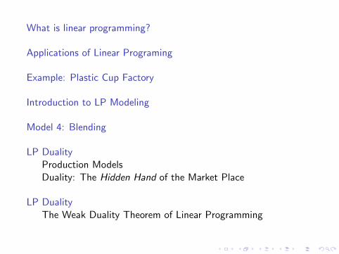
What is linear programming?
Applications of Linear Programing
Example: Plastic Cup Factory
Introduction to LP Modeling
Model 4: Blending
LP DualityProduction ModelsDuality: The Hidden Hand of the Market Place
LP DualityThe Weak Duality Theorem of Linear Programming

What is linear programming (LP)?
A linear program is an optimization problem in finitely manyvariables having a linear objective function and a constraintregion determined by a finite number of linear equality and/orinequality constraints.

What is linear programming (LP)?
A linear program is an optimization problem in finitely manyvariables having a linear objective function and a constraintregion determined by a finite number of linear equality and/orinequality constraints.

Compact Representation
minimize c1x1 + c2x2 + · · ·+ cnxn
subject to ai1xi + ai2x2 + · · ·+ ainxn ≤ αi i = 1, . . . , s
bi1xi + bi2x2 + · · ·+ binxn = βi i = 1, . . . , r .

Vector Inequalities: Componentwise
Let x , y ∈ Rn.
x =
x1x2...xn
y =
y1y2...yn
We write x ≤ y if and only if
xi ≤ yi , i = 1, 2, . . . , n .

Matrix Notation
c1x1 + c2x2 + · · ·+ cnxn = cT x
c =
c1c2...cn
x =
x1x2...xn

Matrix Notation
ai1xi + ai2x2 + · · ·+ ainxn ≤ αi i = 1, . . . , s
⇐⇒Ax ≤ a
A =
a11 a12 . . . a1na21 a22 . . . a2n
......
. . ....
as1 as2 . . . asn
a =
α1
α2...αs

Matrix Notation
bi1xi + bi2x2 + · · ·+ binxn = βi i = 1, . . . , r
⇐⇒Bx = b
B =
b11 b12 . . . b1nb21 b22 . . . b2n
......
. . ....
br1 br2 . . . brn
b =
β1β2...βr

LP’s Matrix Notation
minimize cT xsubject to Ax ≤ a and Bx = b
c =
c1...cn
, a =
α1...αs
, b =
β1...βr
.
A =
a11 . . . a1n. . .
as1 . . . asn
, B =
b11 . . . b1n. . .
br1 . . . brn

LP’s Matrix Notation
minimize cT xsubject to Ax ≤ a and Bx = b
c =
c1...cn
, a =
α1...αs
, b =
β1...βr
.
A =
a11 . . . a1n. . .
as1 . . . asn
, B =
b11 . . . b1n. . .
br1 . . . brn

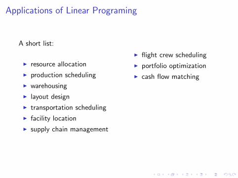
Applications of Linear Programing
A short list:
I resource allocation
I production scheduling
I warehousing
I layout design
I transportation scheduling
I facility location
I supply chain management
I flight crew scheduling
I portfolio optimization
I cash flow matching
I currency exchangearbitrage
I crop scheduling
I diet balancing
I parameter estimation
I . . .

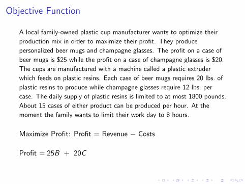
Example: Plastic Cup Factory
A local family-owned plastic cup manufacturer wants to optimizetheir production mix in order to maximize their profit. Theyproduce personalized beer mugs and champagne glasses. Theprofit on a case of beer mugs is $25 while the profit on a case ofchampagne glasses is $20. The cups are manufactured with amachine called a plastic extruder which feeds on plastic resins.Each case of beer mugs requires 20 lbs. of plastic resins to producewhile champagne glasses require 12 lbs. per case. The daily supplyof plastic resins is limited to at most 1800 pounds. About 15 casesof either product can be produced per hour. At the moment thefamily wants to limit their work day to 8 hours.
Model this problem as an LP.

LP Modeling
The four basic steps of LP modeling.
1. Identify and label the decision variables.
2. Determine the objective and use the decision variables towrite an expression for the objective function.
3. Determine the explicit constraints and write a functionalexpression for each of them.
4. Determine the implicit constraints.

Decision Variables
Determining the decision variables is the most difficult part ofmodeling.
To determining these variables it is helpful to put yourself in theshoes of the decision maker, then ask What must he or she knowto do their job.
In the real world, the modeler often follows the decision makeraround for days, weeks, even months at a time recording all of theactions and decisions this person must make.
In this phase of modeling, it is very important to resist thetemptation to make assumptions about the nature of the solution.This last point cannot be over emphasized. Even the mostexperienced modelers occasionally fall into this trap since suchassumptions can enter in very subtle ways.

Decision Variables
Determining the decision variables is the most difficult part ofmodeling.
To determining these variables it is helpful to put yourself in theshoes of the decision maker, then ask What must he or she knowto do their job.
In the real world, the modeler often follows the decision makeraround for days, weeks, even months at a time recording all of theactions and decisions this person must make.
In this phase of modeling, it is very important to resist thetemptation to make assumptions about the nature of the solution.
This last point cannot be over emphasized. Even the mostexperienced modelers occasionally fall into this trap since suchassumptions can enter in very subtle ways.

Decision Variables
Determining the decision variables is the most difficult part ofmodeling.
To determining these variables it is helpful to put yourself in theshoes of the decision maker, then ask What must he or she knowto do their job.
In the real world, the modeler often follows the decision makeraround for days, weeks, even months at a time recording all of theactions and decisions this person must make.
In this phase of modeling, it is very important to resist thetemptation to make assumptions about the nature of the solution.This last point cannot be over emphasized. Even the mostexperienced modelers occasionally fall into this trap since suchassumptions can enter in very subtle ways.

Decision Variables
A local family-owned plastic cup manufacturer wants to optimize their
production mix in order to maximize their profit. They produce
personalized beer mugs and champagne glasses. The profit on a case of
beer mugs is $25 while the profit on a case of champagne glasses is $20.
The cups are manufactured with a machine called a plastic extruder
which feeds on plastic resins. Each case of beer mugs requires 20 lbs. of
plastic resins to produce while champagne glasses require 12 lbs. per
case. The daily supply of plastic resins is limited to at most 1800 pounds.
About 15 cases of either product can be produced per hour. At the
moment the family wants to limit their work day to 8 hours.
B = number of cases of beer mugs produced dailyC = number of cases of champagne glasses produced daily

Decision Variables
A local family-owned plastic cup manufacturer wants to optimize their
production mix in order to maximize their profit. They produce
personalized beer mugs and champagne glasses. The profit on a case of
beer mugs is $25 while the profit on a case of champagne glasses is $20.
The cups are manufactured with a machine called a plastic extruder
which feeds on plastic resins. Each case of beer mugs requires 20 lbs. of
plastic resins to produce while champagne glasses require 12 lbs. per
case. The daily supply of plastic resins is limited to at most 1800 pounds.
About 15 cases of either product can be produced per hour. At the
moment the family wants to limit their work day to 8 hours.
B = number of cases of beer mugs produced daily
C = number of cases of champagne glasses produced daily

Decision Variables
A local family-owned plastic cup manufacturer wants to optimize their
production mix in order to maximize their profit. They produce
personalized beer mugs and champagne glasses. The profit on a case of
beer mugs is $25 while the profit on a case of champagne glasses is $20.
The cups are manufactured with a machine called a plastic extruder
which feeds on plastic resins. Each case of beer mugs requires 20 lbs. of
plastic resins to produce while champagne glasses require 12 lbs. per
case. The daily supply of plastic resins is limited to at most 1800 pounds.
About 15 cases of either product can be produced per hour. At the
moment the family wants to limit their work day to 8 hours.
B = number of cases of beer mugs produced dailyC = number of cases of champagne glasses produced daily

Objective Function
A local family-owned plastic cup manufacturer wants to optimize their
production mix in order to maximize their profit. They produce
personalized beer mugs and champagne glasses. The profit on a case of
beer mugs is $25 while the profit on a case of champagne glasses is $20.
The cups are manufactured with a machine called a plastic extruder
which feeds on plastic resins. Each case of beer mugs requires 20 lbs. of
plastic resins to produce while champagne glasses require 12 lbs. per
case. The daily supply of plastic resins is limited to at most 1800 pounds.
About 15 cases of either product can be produced per hour. At the
moment the family wants to limit their work day to 8 hours.
Maximize Profit: Profit = Revenue − Costs
Profit = 25B + 20C

Objective Function
A local family-owned plastic cup manufacturer wants to optimize their
production mix in order to maximize their profit. They produce
personalized beer mugs and champagne glasses. The profit on a case of
beer mugs is $25 while the profit on a case of champagne glasses is $20.
The cups are manufactured with a machine called a plastic extruder
which feeds on plastic resins. Each case of beer mugs requires 20 lbs. of
plastic resins to produce while champagne glasses require 12 lbs. per
case. The daily supply of plastic resins is limited to at most 1800 pounds.
About 15 cases of either product can be produced per hour. At the
moment the family wants to limit their work day to 8 hours.
Maximize Profit:
Profit = Revenue − Costs
Profit = 25B + 20C

Objective Function
A local family-owned plastic cup manufacturer wants to optimize their
production mix in order to maximize their profit. They produce
personalized beer mugs and champagne glasses. The profit on a case of
beer mugs is $25 while the profit on a case of champagne glasses is $20.
The cups are manufactured with a machine called a plastic extruder
which feeds on plastic resins. Each case of beer mugs requires 20 lbs. of
plastic resins to produce while champagne glasses require 12 lbs. per
case. The daily supply of plastic resins is limited to at most 1800 pounds.
About 15 cases of either product can be produced per hour. At the
moment the family wants to limit their work day to 8 hours.
Maximize Profit: Profit = Revenue − Costs
Profit = 25B + 20C

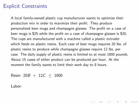
Explicit Constraints
A local family-owned plastic cup manufacturer wants to optimize their
production mix in order to maximize their profit. They produce
personalized beer mugs and champagne glasses. The profit on a case of
beer mugs is $25 while the profit on a case of champagne glasses is $20.
The cups are manufactured with a machine called a plastic extruder
which feeds on plastic resins. Each case of beer mugs requires 20 lbs. of
plastic resins to produce while champagne glasses require 12 lbs. per
case. The daily supply of plastic resins is limited to at most 1800 pounds.
About 15 cases of either product can be produced per hour. At the
moment the family wants to limit their work day to 8 hours.
Resin: 20B + 12C ≤ 1800
Labor: B/15 + C/15 ≤ 8

Explicit Constraints
A local family-owned plastic cup manufacturer wants to optimize their
production mix in order to maximize their profit. They produce
personalized beer mugs and champagne glasses. The profit on a case of
beer mugs is $25 while the profit on a case of champagne glasses is $20.
The cups are manufactured with a machine called a plastic extruder
which feeds on plastic resins. Each case of beer mugs requires 20 lbs. of
plastic resins to produce while champagne glasses require 12 lbs. per
case. The daily supply of plastic resins is limited to at most 1800 pounds.
About 15 cases of either product can be produced per hour. At the
moment the family wants to limit their work day to 8 hours.
Resin:
20B + 12C ≤ 1800
Labor: B/15 + C/15 ≤ 8

Explicit Constraints
A local family-owned plastic cup manufacturer wants to optimize their
production mix in order to maximize their profit. They produce
personalized beer mugs and champagne glasses. The profit on a case of
beer mugs is $25 while the profit on a case of champagne glasses is $20.
The cups are manufactured with a machine called a plastic extruder
which feeds on plastic resins. Each case of beer mugs requires 20 lbs. of
plastic resins to produce while champagne glasses require 12 lbs. per
case. The daily supply of plastic resins is limited to at most 1800 pounds.
About 15 cases of either product can be produced per hour. At the
moment the family wants to limit their work day to 8 hours.
Resin: 20B + 12C ≤ 1800
Labor: B/15 + C/15 ≤ 8
Explicit Constraints
A local family-owned plastic cup manufacturer wants to optimize their
production mix in order to maximize their profit. They produce
personalized beer mugs and champagne glasses. The profit on a case of
beer mugs is $25 while the profit on a case of champagne glasses is $20.
The cups are manufactured with a machine called a plastic extruder
which feeds on plastic resins. Each case of beer mugs requires 20 lbs. of
plastic resins to produce while champagne glasses require 12 lbs. per
case. The daily supply of plastic resins is limited to at most 1800 pounds.
About 15 cases of either product can be produced per hour. At the
moment the family wants to limit their work day to 8 hours.
Resin: 20B + 12C ≤ 1800
Labor:
B/15 + C/15 ≤ 8

Explicit Constraints
A local family-owned plastic cup manufacturer wants to optimize their
production mix in order to maximize their profit. They produce
personalized beer mugs and champagne glasses. The profit on a case of
beer mugs is $25 while the profit on a case of champagne glasses is $20.
The cups are manufactured with a machine called a plastic extruder
which feeds on plastic resins. Each case of beer mugs requires 20 lbs. of
plastic resins to produce while champagne glasses require 12 lbs. per
case. The daily supply of plastic resins is limited to at most 1800 pounds.
About 15 cases of either product can be produced per hour. At the
moment the family wants to limit their work day to 8 hours.
Resin: 20B + 12C ≤ 1800
Labor: B/15 + C/15 ≤ 8

Implicit Constraints
A local family-owned plastic cup manufacturer wants to optimize their
production mix in order to maximize their profit. They produce
personalized beer mugs and champagne glasses. The profit on a case of
beer mugs is $25 while the profit on a case of champagne glasses is $20.
The cups are manufactured with a machine called a plastic extruder
which feeds on plastic resins. Each case of beer mugs requires 20 lbs. of
plastic resins to produce while champagne glasses require 12 lbs. per
case. The daily supply of plastic resins is limited to at most 1800 pounds.
About 15 cases of either product can be produced per hour. At the
moment the family wants to limit their work day to 8 hours.
The decision variables are non-negative: 0 ≤ B, 0 ≤ C

Implicit Constraints
A local family-owned plastic cup manufacturer wants to optimize their
production mix in order to maximize their profit. They produce
personalized beer mugs and champagne glasses. The profit on a case of
beer mugs is $25 while the profit on a case of champagne glasses is $20.
The cups are manufactured with a machine called a plastic extruder
which feeds on plastic resins. Each case of beer mugs requires 20 lbs. of
plastic resins to produce while champagne glasses require 12 lbs. per
case. The daily supply of plastic resins is limited to at most 1800 pounds.
About 15 cases of either product can be produced per hour. At the
moment the family wants to limit their work day to 8 hours.
The decision variables are non-negative:
0 ≤ B, 0 ≤ C

Implicit Constraints
A local family-owned plastic cup manufacturer wants to optimize their
production mix in order to maximize their profit. They produce
personalized beer mugs and champagne glasses. The profit on a case of
beer mugs is $25 while the profit on a case of champagne glasses is $20.
The cups are manufactured with a machine called a plastic extruder
which feeds on plastic resins. Each case of beer mugs requires 20 lbs. of
plastic resins to produce while champagne glasses require 12 lbs. per
case. The daily supply of plastic resins is limited to at most 1800 pounds.
About 15 cases of either product can be produced per hour. At the
moment the family wants to limit their work day to 8 hours.
The decision variables are non-negative: 0 ≤ B, 0 ≤ C

The Plastic Cup Factory LP Model
maximize 25B + 20C
subject to 20B + 12C ≤ 1800
115B + 1
15C ≤ 8
0 ≤ B,C

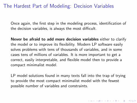
The Hardest Part of Modeling: Decision Variables
Once again, the first step in the modeling process, identification ofthe decision variables, is always the most difficult.
Never be afraid to add more decision variables either to clarifythe model or to improve its flexibility. Modern LP software easilysolves problems with tens of thousands of variables, and in somecases tens of millions of variables. It is more important to get acorrect, easily interpretable, and flexible model then to provide acompact minimalist model.
LP model solutions found in many texts fall into the trap of tryingto provide the most compact minimalist model with the fewestpossible number of variables and constraints.Do not repeat this error in developing your own models.
The Hardest Part of Modeling: Decision Variables
Once again, the first step in the modeling process, identification ofthe decision variables, is always the most difficult.
Never be afraid to add more decision variables either to clarifythe model or to improve its flexibility. Modern LP software easilysolves problems with tens of thousands of variables, and in somecases tens of millions of variables. It is more important to get acorrect, easily interpretable, and flexible model then to provide acompact minimalist model.
LP model solutions found in many texts fall into the trap of tryingto provide the most compact minimalist model with the fewestpossible number of variables and constraints.
Do not repeat this error in developing your own models.

The Hardest Part of Modeling: Decision Variables
Once again, the first step in the modeling process, identification ofthe decision variables, is always the most difficult.
Never be afraid to add more decision variables either to clarifythe model or to improve its flexibility. Modern LP software easilysolves problems with tens of thousands of variables, and in somecases tens of millions of variables. It is more important to get acorrect, easily interpretable, and flexible model then to provide acompact minimalist model.
LP model solutions found in many texts fall into the trap of tryingto provide the most compact minimalist model with the fewestpossible number of variables and constraints.Do not repeat this error in developing your own models.

Model 4: Blending
A company makes a blend consisting of two chemicals, 1 and 2, in the
ratio 5:2 by weight. These chemical can be manufactured by three
different processes using two different raw materials and a fuel.
Production data are given in the table below. For how much time should
each process be run in order to maximize the total amount of blend
manufactured?
Requirements per Unit Time Output per Unit TimeRaw Mat. 1 Raw Mat. 2 Fuel Chem. 1 Chem. 2
Process (units) (units) (units) (units) (units)
1 9 5 50 9 62 6 8 75 7 103 4 11 100 10 6
Amountavailable 200 400 1850

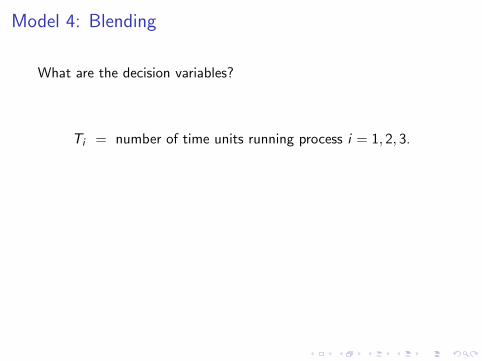
Model 4: Blending
What are the decision variables?
Ti = number of time units running process i = 1, 2, 3.
What is the objective functions?
maximize Blend = B
Model 4: Blending
What are the decision variables?
Ti = number of time units running process i = 1, 2, 3.
What is the objective functions?
maximize Blend = B
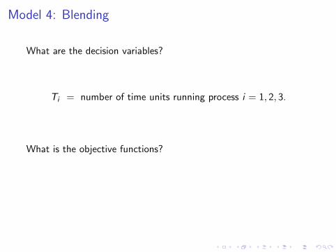
Model 4: Blending
What are the decision variables?
Ti = number of time units running process i = 1, 2, 3.
What is the objective functions?
maximize Blend = B

Model 4: Blending
What are the decision variables?
Ti = number of time units running process i = 1, 2, 3.
What is the objective functions?
maximize Blend = B

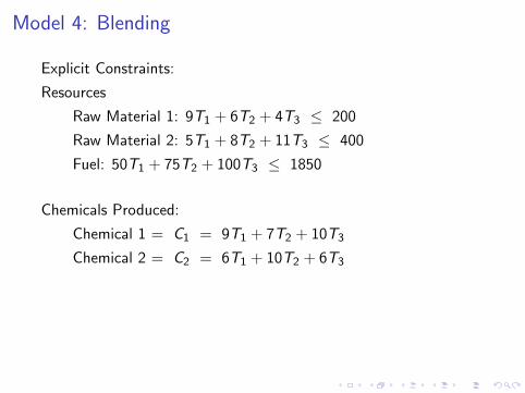
Model 4: Blending
Explicit Constraints:
Resources
Raw Material 1: 9T1 + 6T2 + 4T3 ≤ 200
Raw Material 2: 5T1 + 8T2 + 11T3 ≤ 400
Fuel: 50T1 + 75T2 + 100T3 ≤ 1850
Chemicals Produced:
Chemical 1 = C1 = 9T1 + 7T2 + 10T3
Chemical 2 = C2 = 6T1 + 10T2 + 6T3
Blend: 57B ≤ C1 and 2
7B ≤ C2
Implicit Constraints: 0 ≤ B, 0 ≤ Ti , i = 1, 2, 3, 0 ≤ Cj , j = 1, 2

Model 4: Blending
Explicit Constraints:
Resources
Raw Material 1: 9T1 + 6T2 + 4T3 ≤ 200
Raw Material 2: 5T1 + 8T2 + 11T3 ≤ 400
Fuel: 50T1 + 75T2 + 100T3 ≤ 1850
Chemicals Produced:
Chemical 1 = C1 = 9T1 + 7T2 + 10T3
Chemical 2 = C2 = 6T1 + 10T2 + 6T3
Blend:
57B ≤ C1 and 2
7B ≤ C2
Implicit Constraints: 0 ≤ B, 0 ≤ Ti , i = 1, 2, 3, 0 ≤ Cj , j = 1, 2

Model 4: Blending
Explicit Constraints:
Resources
Raw Material 1: 9T1 + 6T2 + 4T3 ≤ 200
Raw Material 2: 5T1 + 8T2 + 11T3 ≤ 400
Fuel: 50T1 + 75T2 + 100T3 ≤ 1850
Chemicals Produced:
Chemical 1 = C1 = 9T1 + 7T2 + 10T3
Chemical 2 = C2 = 6T1 + 10T2 + 6T3
Blend: 57B ≤ C1
and 27B ≤ C2
Implicit Constraints: 0 ≤ B, 0 ≤ Ti , i = 1, 2, 3, 0 ≤ Cj , j = 1, 2

Model 4: Blending
Explicit Constraints:
Resources
Raw Material 1: 9T1 + 6T2 + 4T3 ≤ 200
Raw Material 2: 5T1 + 8T2 + 11T3 ≤ 400
Fuel: 50T1 + 75T2 + 100T3 ≤ 1850
Chemicals Produced:
Chemical 1 = C1 = 9T1 + 7T2 + 10T3
Chemical 2 = C2 = 6T1 + 10T2 + 6T3
Blend: 57B ≤ C1 and 2
7B ≤ C2
Implicit Constraints: 0 ≤ B, 0 ≤ Ti , i = 1, 2, 3, 0 ≤ Cj , j = 1, 2

Model 4: Blending
Explicit Constraints:
Resources
Raw Material 1: 9T1 + 6T2 + 4T3 ≤ 200
Raw Material 2: 5T1 + 8T2 + 11T3 ≤ 400
Fuel: 50T1 + 75T2 + 100T3 ≤ 1850
Chemicals Produced:
Chemical 1 = C1 = 9T1 + 7T2 + 10T3
Chemical 2 = C2 = 6T1 + 10T2 + 6T3
Blend: 57B ≤ C1 and 2
7B ≤ C2
Implicit Constraints: 0 ≤ B, 0 ≤ Ti , i = 1, 2, 3, 0 ≤ Cj , j = 1, 2

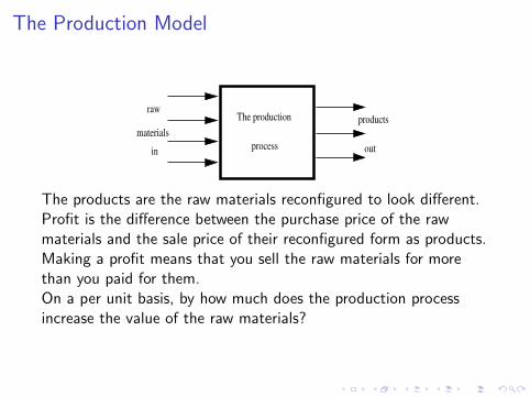
The Production Model
in
materials
rawproducts
out
The production
process
The products are the raw materials reconfigured to look different.Profit is the difference between the purchase price of the rawmaterials and the sale price of their reconfigured form as products.Making a profit means that you sell the raw materials for morethan you paid for them.On a per unit basis, by how much does the production processincrease the value of the raw materials?

The Production Model
in
materials
rawproducts
out
The production
process
The products are the raw materials reconfigured to look different.
Profit is the difference between the purchase price of the rawmaterials and the sale price of their reconfigured form as products.Making a profit means that you sell the raw materials for morethan you paid for them.On a per unit basis, by how much does the production processincrease the value of the raw materials?

The Production Model
in
materials
rawproducts
out
The production
process
The products are the raw materials reconfigured to look different.Profit is the difference between the purchase price of the rawmaterials and the sale price of their reconfigured form as products.
Making a profit means that you sell the raw materials for morethan you paid for them.On a per unit basis, by how much does the production processincrease the value of the raw materials?

The Production Model
in
materials
rawproducts
out
The production
process
The products are the raw materials reconfigured to look different.Profit is the difference between the purchase price of the rawmaterials and the sale price of their reconfigured form as products.Making a profit means that you sell the raw materials for morethan you paid for them.
On a per unit basis, by how much does the production processincrease the value of the raw materials?
The Production Model
in
materials
rawproducts
out
The production
process
The products are the raw materials reconfigured to look different.Profit is the difference between the purchase price of the rawmaterials and the sale price of their reconfigured form as products.Making a profit means that you sell the raw materials for morethan you paid for them.On a per unit basis, by how much does the production processincrease the value of the raw materials?

Hidden Hand of the Market Place: Duality
In the market place there is competition for raw materials, or theinputs to production. This collective competition is the hiddenhand that sets the price for goods in the market place.
Is there a mathematical model for how these prices are set?
Let us think of the market as a separate agent in the market place.It is the agent that owns and sells the raw materials of production.
The goal of the market is to make the most money possible fromits resources by setting the highest prices possible for them.
The market does not want to put the producers out of business, itjust wants to take all of their profit.
How can we model this mathematically?

Hidden Hand of the Market Place: Duality
We answer this question in the context of the Plastic Cup Factory.
A local family-owned plastic cup manufacturer wants to optimize their
production mix in order to maximize their profit. They produce
personalized beer mugs and champagne glasses. The profit on a case of
beer mugs is $25 while the profit on a case of champagne glasses is $20.
The cups are manufactured with a machine called a plastic extruder
which feeds on plastic resins. Each case of beer mugs requires 20 lbs. of
plastic resins to produce while champagne glasses require 12 lbs. per
case. The daily supply of plastic resins is limited to at most 1800 pounds.
About 15 cases of either product can be produced per hour. At the
moment the family wants to limit their work day to 8 hours.

Hidden Hand of the Market Place: Duality
By how much should the market increase the sale price of plasticresin and hourly labor in order to wipe out the profit for the PlasticCup Factory?
Define
0 ≤ y1 = price increase for a pound of resin
0 ≤ y2 = price increase for an hour of labor
These price increases should wipe out the per unit profitability forcases of both beer mugs and champagne glasses.

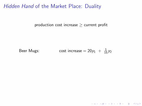
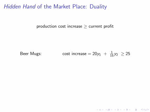
Hidden Hand of the Market Place: Duality
production cost increase ≥ current profit
Beer Mugs: cost increase = 20y1 + 115y2 ≥ 25
Champagne Glasses: cost increase = 12y1 + 115y2 ≥ 20

Hidden Hand of the Market Place: Duality
production cost increase ≥ current profit
Beer Mugs: cost increase =
20y1 + 115y2 ≥ 25
Champagne Glasses: cost increase = 12y1 + 115y2 ≥ 20
Hidden Hand of the Market Place: Duality
production cost increase ≥ current profit
Beer Mugs: cost increase = 20y1 + 115y2
≥ 25
Champagne Glasses: cost increase = 12y1 + 115y2 ≥ 20
Hidden Hand of the Market Place: Duality
production cost increase ≥ current profit
Beer Mugs: cost increase = 20y1 + 115y2 ≥ 25
Champagne Glasses: cost increase = 12y1 + 115y2 ≥ 20

Hidden Hand of the Market Place: Duality
production cost increase ≥ current profit
Beer Mugs: cost increase = 20y1 + 115y2 ≥ 25
Champagne Glasses:
cost increase = 12y1 + 115y2 ≥ 20

Hidden Hand of the Market Place: Duality
production cost increase ≥ current profit
Beer Mugs: cost increase = 20y1 + 115y2 ≥ 25
Champagne Glasses: cost increase =
12y1 + 115y2 ≥ 20

Hidden Hand of the Market Place: Duality
production cost increase ≥ current profit
Beer Mugs: cost increase = 20y1 + 115y2 ≥ 25
Champagne Glasses: cost increase = 12y1 + 115y2
≥ 20

Hidden Hand of the Market Place: Duality
production cost increase ≥ current profit
Beer Mugs: cost increase = 20y1 + 115y2 ≥ 25
Champagne Glasses: cost increase = 12y1 + 115y2 ≥ 20

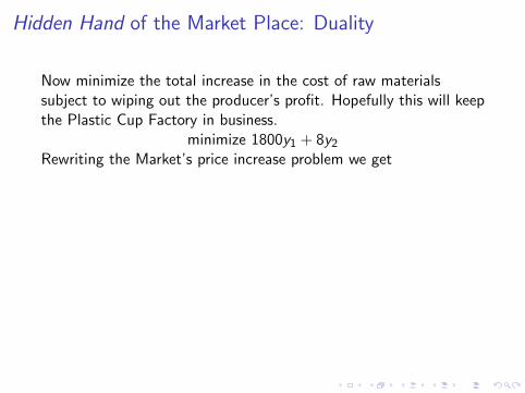
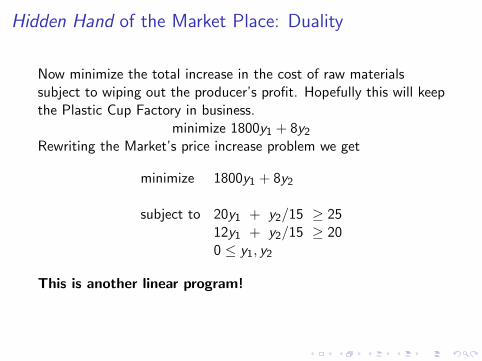
Hidden Hand of the Market Place: Duality
Now minimize the total increase in the cost of raw materialssubject to wiping out the producer’s profit. Hopefully this will keepthe Plastic Cup Factory in business.
minimize 1800y1 + 8y2Rewriting the Market’s price increase problem we get
minimize 1800y1 + 8y2
subject to 20y1 + y2/15 ≥ 2512y1 + y2/15 ≥ 200 ≤ y1, y2
This is another linear program!Let us compare this LP with the original LP.

Hidden Hand of the Market Place: Duality
Now minimize the total increase in the cost of raw materialssubject to wiping out the producer’s profit. Hopefully this will keepthe Plastic Cup Factory in business.
minimize 1800y1 + 8y2
Rewriting the Market’s price increase problem we get
minimize 1800y1 + 8y2
subject to 20y1 + y2/15 ≥ 2512y1 + y2/15 ≥ 200 ≤ y1, y2
This is another linear program!Let us compare this LP with the original LP.
Hidden Hand of the Market Place: Duality
Now minimize the total increase in the cost of raw materialssubject to wiping out the producer’s profit. Hopefully this will keepthe Plastic Cup Factory in business.
minimize 1800y1 + 8y2Rewriting the Market’s price increase problem we get
minimize 1800y1 + 8y2
subject to 20y1 + y2/15 ≥ 2512y1 + y2/15 ≥ 200 ≤ y1, y2
This is another linear program!Let us compare this LP with the original LP.

Hidden Hand of the Market Place: Duality
Now minimize the total increase in the cost of raw materialssubject to wiping out the producer’s profit. Hopefully this will keepthe Plastic Cup Factory in business.
minimize 1800y1 + 8y2Rewriting the Market’s price increase problem we get
minimize 1800y1 + 8y2
subject to 20y1 + y2/15 ≥ 2512y1 + y2/15 ≥ 200 ≤ y1, y2
This is another linear program!Let us compare this LP with the original LP.
Hidden Hand of the Market Place: Duality
Now minimize the total increase in the cost of raw materialssubject to wiping out the producer’s profit. Hopefully this will keepthe Plastic Cup Factory in business.
minimize 1800y1 + 8y2Rewriting the Market’s price increase problem we get
minimize 1800y1 + 8y2
subject to 20y1 + y2/15 ≥ 2512y1 + y2/15 ≥ 200 ≤ y1, y2
This is another linear program!
Let us compare this LP with the original LP.

Hidden Hand of the Market Place: Duality
Now minimize the total increase in the cost of raw materialssubject to wiping out the producer’s profit. Hopefully this will keepthe Plastic Cup Factory in business.
minimize 1800y1 + 8y2Rewriting the Market’s price increase problem we get
minimize 1800y1 + 8y2
subject to 20y1 + y2/15 ≥ 2512y1 + y2/15 ≥ 200 ≤ y1, y2
This is another linear program!Let us compare this LP with the original LP.

Linear Programming Duality
Primal: max 25B + 20C
s.t. 20B + 12C ≤ 1800
115B + 1
15C ≤ 8
0 ≤ B,C
Dual: min 1800y1 + 8y2
s.t. 20y1 + 115y2 ≥ 25
12y1 + 115y2 ≥ 20
0 ≤ y1, y2

Linear Programming Duality
Primal:
max 25B + 20C
s.t. 20B + 12C ≤ 1800
115B + 1
15C ≤ 8
0 ≤ B,C
Dual: min 1800y1 + 8y2
s.t. 20y1 + 115y2 ≥ 25
12y1 + 115y2 ≥ 20
0 ≤ y1, y2

Linear Programming Duality
Primal: max 25B + 20C
s.t. 20B + 12C ≤ 1800
115B + 1
15C ≤ 8
0 ≤ B,C
Dual: min 1800y1 + 8y2
s.t. 20y1 + 115y2 ≥ 25
12y1 + 115y2 ≥ 20
0 ≤ y1, y2

Linear Programming Duality
Primal: max 25B + 20C
s.t. 20B + 12C ≤ 1800
115B + 1
15C ≤ 8
0 ≤ B,C
Dual:
min 1800y1 + 8y2
s.t. 20y1 + 115y2 ≥ 25
12y1 + 115y2 ≥ 20
0 ≤ y1, y2

Linear Programming Duality
Primal: max 25B + 20C
s.t. 20B + 12C ≤ 1800
115B + 1
15C ≤ 8
0 ≤ B,C
Dual: min 1800y1 + 8y2
s.t. 20y1 + 115y2 ≥ 25
12y1 + 115y2 ≥ 20
0 ≤ y1, y2

Linear Programming Duality: Matrix Notation
P
Primal: max cT x
s.t. Ax ≤ b
0 ≤ x
D
Dual: min bT y
s.t. AT y ≥ c
0 ≤ y

The Weak Duality Theorem of Linear Programming
Theorem: [Weak Duality Theorem]
If x ∈ Rn is feasible for P and y ∈ Rm is feasible for D, then
cT x ≤ yTAx ≤ bT y .
Thus, if P is unbounded, then D is necessarily infeasible, and if Dis unbounded, then P is necessarily infeasible.
Moreover, if cT x = bT y with x feasible for P and y feasible for D,then x must solve P and y must solve D.

The Weak Duality Theorem of Linear Programming
Theorem: [Weak Duality Theorem]If x ∈ Rn is feasible for P and y ∈ Rm is feasible for D, then
cT x ≤ yTAx ≤ bT y .
Thus, if P is unbounded, then D is necessarily infeasible, and if Dis unbounded, then P is necessarily infeasible.
Moreover, if cT x = bT y with x feasible for P and y feasible for D,then x must solve P and y must solve D.

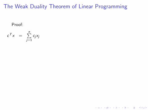
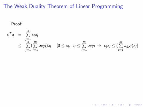
The Weak Duality Theorem of Linear Programming
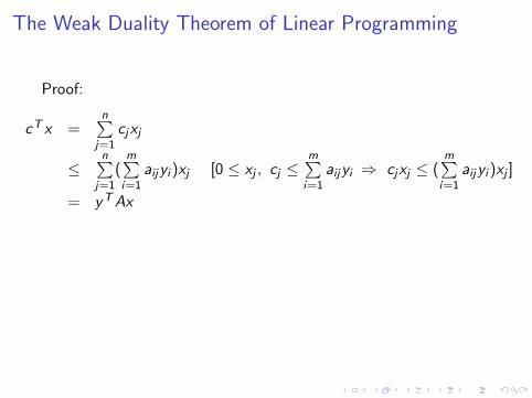
Proof:
cT x =n∑
j=1cjxj
≤n∑
j=1(m∑i=1
aijyi )xj [0 ≤ xj , cj ≤m∑i=1
aijyi ⇒ cjxj ≤ (m∑i=1
aijyi )xj ]
= yTAx
=m∑i=1
(n∑
j=1aijxj)yi
≤m∑i=1
biyi [0 ≤ yi ,n∑
j=1aijxj ≤ bi ⇒ (
n∑j=1
aijxj)yi ≤ biyi ]
= bT y
The Weak Duality Theorem of Linear Programming
Proof:
cT x =n∑
j=1cjxj
≤n∑
j=1(m∑i=1
aijyi )xj [0 ≤ xj , cj ≤m∑i=1
aijyi ⇒ cjxj ≤ (m∑i=1
aijyi )xj ]
= yTAx
=m∑i=1
(n∑
j=1aijxj)yi
≤m∑i=1
biyi [0 ≤ yi ,n∑
j=1aijxj ≤ bi ⇒ (
n∑j=1
aijxj)yi ≤ biyi ]
= bT y
The Weak Duality Theorem of Linear Programming
Proof:
cT x =n∑
j=1cjxj
≤n∑
j=1(m∑i=1
aijyi )xj [0 ≤ xj , cj ≤m∑i=1
aijyi ⇒ cjxj ≤ (m∑i=1
aijyi )xj ]
= yTAx
=m∑i=1
(n∑
j=1aijxj)yi
≤m∑i=1
biyi [0 ≤ yi ,n∑
j=1aijxj ≤ bi ⇒ (
n∑j=1
aijxj)yi ≤ biyi ]
= bT y
The Weak Duality Theorem of Linear Programming
Proof:
cT x =n∑
j=1cjxj
≤n∑
j=1(m∑i=1
aijyi )xj [0 ≤ xj , cj ≤m∑i=1
aijyi ⇒ cjxj ≤ (m∑i=1
aijyi )xj ]
= yTAx
=m∑i=1
(n∑
j=1aijxj)yi
≤m∑i=1
biyi [0 ≤ yi ,n∑
j=1aijxj ≤ bi ⇒ (
n∑j=1
aijxj)yi ≤ biyi ]
= bT y

The Weak Duality Theorem of Linear Programming
Proof:
cT x =n∑
j=1cjxj
≤n∑
j=1(m∑i=1
aijyi )xj [0 ≤ xj , cj ≤m∑i=1
aijyi ⇒ cjxj ≤ (m∑i=1
aijyi )xj ]
= yTAx
=m∑i=1
(n∑
j=1aijxj)yi
≤m∑i=1
biyi [0 ≤ yi ,n∑
j=1aijxj ≤ bi ⇒ (
n∑j=1
aijxj)yi ≤ biyi ]
= bT y

The Weak Duality Theorem of Linear Programming
Proof:
cT x =n∑
j=1cjxj
≤n∑
j=1(m∑i=1
aijyi )xj [0 ≤ xj , cj ≤m∑i=1
aijyi ⇒ cjxj ≤ (m∑i=1
aijyi )xj ]
= yTAx
=m∑i=1
(n∑
j=1aijxj)yi
≤m∑i=1
biyi [0 ≤ yi ,n∑
j=1aijxj ≤ bi ⇒ (
n∑j=1
aijxj)yi ≤ biyi ]
= bT y

The Weak Duality Theorem of Linear Programming
Proof:
cT x =n∑
j=1cjxj
≤n∑
j=1(m∑i=1
aijyi )xj [0 ≤ xj , cj ≤m∑i=1
aijyi ⇒ cjxj ≤ (m∑i=1
aijyi )xj ]
= yTAx
=m∑i=1
(n∑
j=1aijxj)yi
≤m∑i=1
biyi [0 ≤ yi ,n∑
j=1aijxj ≤ bi ⇒ (
n∑j=1
aijxj)yi ≤ biyi ]
= bT y

Test the WDT on the Plastic Cup Factory
Optimal Solution =
[4575
]Marginal Values =
[5/8
375/2
]Dual: min 1800y1 + 8y2
s.t. 20y1 + 115y2 ≥ 25
12y1 + 115y2 ≥ 20
0 ≤ y1, y2Dual feasibility of the marginal values:
0 ≤ 5
8
,
0 ≤ 375
2, 20 · 5
8+
1
15· 375
2≥ 25, 12 · 5
8+
1
15· 375
2≥ 20
Equivalence of primal-dual objectives (WDT):
cT x = 25 · 45 + 20 · 75 = 2625 = 1800 · 5
8+ 8 · 375
2= bT y

Test the WDT on the Plastic Cup Factory
Optimal Solution =
[4575
]Marginal Values =
[5/8
375/2
]
Dual: min 1800y1 + 8y2s.t. 20y1 + 1
15y2 ≥ 2512y1 + 1
15y2 ≥ 200 ≤ y1, y2
Dual feasibility of the marginal values:
0 ≤ 5
8
,
0 ≤ 375
2, 20 · 5
8+
1
15· 375
2≥ 25, 12 · 5
8+
1
15· 375
2≥ 20
Equivalence of primal-dual objectives (WDT):
cT x = 25 · 45 + 20 · 75 = 2625 = 1800 · 5
8+ 8 · 375
2= bT y

Test the WDT on the Plastic Cup Factory
Optimal Solution =
[4575
]Marginal Values =
[5/8
375/2
]Dual: min 1800y1 + 8y2
s.t. 20y1 + 115y2 ≥ 25
12y1 + 115y2 ≥ 20
0 ≤ y1, y2
Dual feasibility of the marginal values:
0 ≤ 5
8
,
0 ≤ 375
2, 20 · 5
8+
1
15· 375
2≥ 25, 12 · 5
8+
1
15· 375
2≥ 20
Equivalence of primal-dual objectives (WDT):
cT x = 25 · 45 + 20 · 75 = 2625 = 1800 · 5
8+ 8 · 375
2= bT y

Test the WDT on the Plastic Cup Factory
Optimal Solution =
[4575
]Marginal Values =
[5/8
375/2
]Dual: min 1800y1 + 8y2
s.t. 20y1 + 115y2 ≥ 25
12y1 + 115y2 ≥ 20
0 ≤ y1, y2Dual feasibility of the marginal values:
0 ≤ 5
8
,
0 ≤ 375
2, 20 · 5
8+
1
15· 375
2≥ 25, 12 · 5
8+
1
15· 375
2≥ 20
Equivalence of primal-dual objectives (WDT):
cT x = 25 · 45 + 20 · 75 = 2625 = 1800 · 5
8+ 8 · 375
2= bT y

Test the WDT on the Plastic Cup Factory
Optimal Solution =
[4575
]Marginal Values =
[5/8
375/2
]Dual: min 1800y1 + 8y2
s.t. 20y1 + 115y2 ≥ 25
12y1 + 115y2 ≥ 20
0 ≤ y1, y2Dual feasibility of the marginal values:
0 ≤ 5
8,
0 ≤ 375
2, 20 · 5
8+
1
15· 375
2≥ 25, 12 · 5
8+
1
15· 375
2≥ 20
Equivalence of primal-dual objectives (WDT):
cT x = 25 · 45 + 20 · 75 = 2625 = 1800 · 5
8+ 8 · 375
2= bT y

Test the WDT on the Plastic Cup Factory
Optimal Solution =
[4575
]Marginal Values =
[5/8
375/2
]Dual: min 1800y1 + 8y2
s.t. 20y1 + 115y2 ≥ 25
12y1 + 115y2 ≥ 20
0 ≤ y1, y2Dual feasibility of the marginal values:
0 ≤ 5
8, 0 ≤ 375
2,
20 · 58
+1
15· 375
2≥ 25, 12 · 5
8+
1
15· 375
2≥ 20
Equivalence of primal-dual objectives (WDT):
cT x = 25 · 45 + 20 · 75 = 2625 = 1800 · 5
8+ 8 · 375
2= bT y

Test the WDT on the Plastic Cup Factory
Optimal Solution =
[4575
]Marginal Values =
[5/8
375/2
]Dual: min 1800y1 + 8y2
s.t. 20y1 + 115y2 ≥ 25
12y1 + 115y2 ≥ 20
0 ≤ y1, y2Dual feasibility of the marginal values:
0 ≤ 5
8, 0 ≤ 375
2, 20 · 5
8+
1
15· 375
2≥ 25,
12 · 58
+1
15· 375
2≥ 20
Equivalence of primal-dual objectives (WDT):
cT x = 25 · 45 + 20 · 75 = 2625 = 1800 · 5
8+ 8 · 375
2= bT y

Test the WDT on the Plastic Cup Factory
Optimal Solution =
[4575
]Marginal Values =
[5/8
375/2
]Dual: min 1800y1 + 8y2
s.t. 20y1 + 115y2 ≥ 25
12y1 + 115y2 ≥ 20
0 ≤ y1, y2Dual feasibility of the marginal values:
0 ≤ 5
8, 0 ≤ 375
2, 20 · 5
8+
1
15· 375
2≥ 25, 12 · 5
8+
1
15· 375
2≥ 20
Equivalence of primal-dual objectives (WDT):
cT x = 25 · 45 + 20 · 75 = 2625 = 1800 · 5
8+ 8 · 375
2= bT y

Test the WDT on the Plastic Cup Factory
Optimal Solution =
[4575
]Marginal Values =
[5/8
375/2
]Dual: min 1800y1 + 8y2
s.t. 20y1 + 115y2 ≥ 25
12y1 + 115y2 ≥ 20
0 ≤ y1, y2Dual feasibility of the marginal values:
0 ≤ 5
8, 0 ≤ 375
2, 20 · 5
8+
1
15· 375
2≥ 25, 12 · 5
8+
1
15· 375
2≥ 20
Equivalence of primal-dual objectives (WDT):
cT x = 25 · 45 + 20 · 75 = 2625
= 1800 · 5
8+ 8 · 375
2= bT y

Test the WDT on the Plastic Cup Factory
Optimal Solution =
[4575
]Marginal Values =
[5/8
375/2
]Dual: min 1800y1 + 8y2
s.t. 20y1 + 115y2 ≥ 25
12y1 + 115y2 ≥ 20
0 ≤ y1, y2Dual feasibility of the marginal values:
0 ≤ 5
8, 0 ≤ 375
2, 20 · 5
8+
1
15· 375
2≥ 25, 12 · 5
8+
1
15· 375
2≥ 20
Equivalence of primal-dual objectives (WDT):
cT x = 25 · 45 + 20 · 75 = 2625 = 1800 · 5
8+ 8 · 375
2= bT y

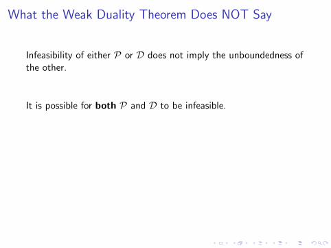
What the Weak Duality Theorem Does NOT Say
Infeasibility of either P or D does not imply the unboundedness ofthe other.
It is possible for both P and D to be infeasible.
Example:maximize 2x1 − x2
x1 − x2 ≤ 1−x1 + x2 ≤ −2
0 ≤ x1, x2

What the Weak Duality Theorem Does NOT Say
Infeasibility of either P or D does not imply the unboundedness ofthe other.
It is possible for both P and D to be infeasible.
Example:maximize 2x1 − x2
x1 − x2 ≤ 1−x1 + x2 ≤ −2
0 ≤ x1, x2
What the Weak Duality Theorem Does NOT Say
Infeasibility of either P or D does not imply the unboundedness ofthe other.
It is possible for both P and D to be infeasible.
Example:maximize 2x1 − x2
x1 − x2 ≤ 1−x1 + x2 ≤ −2
0 ≤ x1, x2

What the Weak Duality Theorem Does NOT Say
Infeasibility of either P or D does not imply the unboundedness ofthe other.
It is possible for both P and D to be infeasible.
Example:maximize 2x1 − x2
x1 − x2 ≤ 1−x1 + x2 ≤ −2
0 ≤ x1, x2