linear regression models cgfm

Chaohui Guo & Friederike Meyer

PATTERN RECOGNITION AND MACHINE LEARNINGCHAPTER 3: LINEAR MODELS FOR REGRESSION

Purposes of linear regression

• Specifying relationship between independent variables (input vector x) and dependent variables (target values t)

• Assumption: Targets are noisy realization of an underlying functional relationship

• Goal: model the predictive distribution p(t|x)

• A general linear model (GLM) explains this relationship in terms of a linear combination of the IV + error: tn = y(xn,β) + εn

GLM: Illustration of matrix form

=

e+y X

N

1

N N

1 1p

p

eXy eXy

),0(~ 2INe ),0(~ 2INe

N: number of scansp: number of regressors

Parameter estimation

eXy

= +

e

2

1

Ordinary least squares estimation

(OLS) (assuming i.i.d. error):

yXXX TT 1)(ˆ

Objective:estimate β tominimize

N

tte

1

2

y X

ye

Design space defined by X

x1

x2

GLM: A geometric perspective

PIRRye

PIR

Rye

ˆ Xy

yXXX TT 1)(ˆ yXXX TT 1)(ˆ

TT XXXXPPyy

1)(

ˆ

TT XXXXP

Pyy1)(

ˆ

Residual forming matrix

R

Projection matrix P

OLS estimates

LS es mate of the data ∟ projec on of data vector onto design matrix space

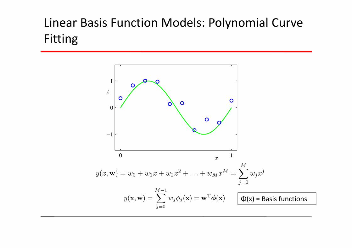
Linear Basis Function Models: Polynomial Curve Fitting

Φ(x) = Basis functions

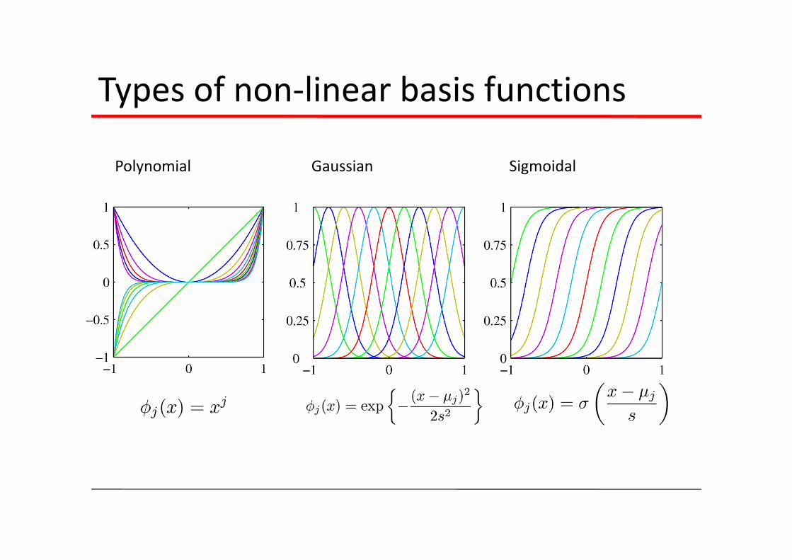
Types of non‐linear basis functions

Polynomial Gaussian Sigmoidal

Estimation of ω: Classical (frequentist) techniques

• Using an “estimator” to determine specific value for parameter vector ω e.g. Sum‐of‐squares error function (SSQ):

• Minimizing function in respect to ω: ω*• t = y(x, ω*)

Reducing over‐fitting: Regularized Least Squares

Control of over‐fitting: Regularization of error function

which is minimized by

Data‐dependent error + Regularization term

λ : regularization coefficient.

OLS‐solution + extension

(λ/2)ωTω

Regularized Least Squares

Applying more general regularizer:

How to choose appropriate λ‐value?

Classical techniques: Maximum Likelihood and Least Squares

• Assume observations from a deterministic function with added Gaussian noise:

which implies a Gaussian conditional distribution:

• Given observed inputs, (independently drawn), and targets, , we obtain the likelihood function

where

Classical techniques: Maximum Likelihood and Least Squares

Taking the logarithm, we get

Computing the gradient and setting it to zero yields

Solving for w , we get

OLS estimate

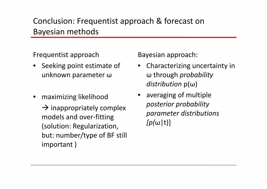
Conclusion: Frequentist approach & forecast on Bayesian methods

Frequentist approach • Seeking point estimate of

unknown parameter ω

• maximizing likelihood inappropriately complex models and over‐fitting (solution: Regularization, but: number/type of BF still important )

Bayesian approach: • Characterizing uncertainty in

ω through probabilitydistribution p(ω)

• averaging of multiple posterior probability parameter distributions [p(ω|t)]

Bayesian linear regression: Parameter distribution

• β: assumed known constant

• Likelihood function: p(t|ω) with Gaussian noise exponential of quadratic function of ω

• Gaussian prior: p(ω) = N(ω|m0,S0)

• Gaussian posterior: p(ω|t) = [p(D|ω)*p(ω)]/p(D) p(ω|t) = N(ω|mN,SN) mN= SN (S0‐1m0 + βΦTt) SN = S0‐1 + βΦTΦ

Bayesian Linear Regression: Common cases

• A common choice for the prior is a zero‐mean isotropic Gaussian:

for which

•Maximization of posterior distribution = minimization ofSSQ with addition of quadratic error term (λ = α/β)

Bayesian Linear Regression: An Example of sequential learning

• Linear model: y(x,w) = ω0 + ω1x (straight‐line fitting)

• Generation of synthetic data: f(y,a) = a0 + a1x a0 = ‐0.3, a1 = 0.5 Gaussian noise(std, β‐1) = 0.2 β = (1/0.2)2 = 25 α = 2.0 U(x|‐1,1)


Likelihoodp(t|x,ω)

Prior[p(ω)] (+p(t|x,ω) gives)/Posterior p(ω|t)

Data Space (6 samples y(x,w) drawn from posterior distribution of ω)


Likelihood Prior/Posterior Data Space

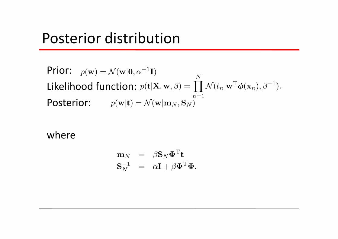
Posterior distribution

Prior: Likelihood function: Posterior:

where

Predictive Distribution (1)

Predict t for new values x:

where

Sum rule

Product rule

Predictive Distribution (2)Example: Sinusoidal data, 9 Gaussian basis functions

Predictive Distribution (3)Example: Sinusoidal data, 9 Gaussian basis functions

25 data points

Bayesian Model Comparison (1)

How do we choose the ‘right’ model? L models

Bayes Factor: ratio of evidence for two models

Posterior Prior Model evidence


Simple situation:For a given model with a single parameter, , consider the approximation

where the posterior is assumed to be sharply peaked, and prioris flat.


Taking logarithms, we obtain

With M parameters, all assumed to have the same ratio , we get

Negative

Negative and linear in M.


data fit and model complexity, favour intermediate complexity:

D1 D2

Practical use

‐How good are these assumptions?‐What other functions to be use?‐Bayesian framework avoids the problem of over‐fitting and allows models to be

compared on the basis of the training data alone. However, due to the dependence on the priors, a practical application is to keep an independent test set of data.

Predictive distribution

Predictive distribution

A simpler approximation, known as model selection, is to use the model with the highest evidence.

The Evidence Approximation (1)

The fully Bayesian predictive distribution is given by

but this integral is intractable. Approximate with

where is the mode of , which is assumed to be sharply peaked; a.k.a. evidence approximation.


From Bayes’ theorem we have

and if we assume prior to be flat we see that

Final evidence function:


To maximise , first derivative respect to

Derivative Respect to

Iterative procedure: Initial choice for and , calculate for mN and r. these values are re‐estimate and , until convergence.


In the limit , and we can consider using the easy‐to‐compute approximation


Example: sinusoidal data,

Discussion

‐ Are they always consistent?‐ Bayesian vs. Frequencist

‐ Sequential learning‐ Model selection‐ How they different with a flat prior?

Model Selection(1.3)

Cross‐Validation

Akaike information criterion (AIC) :

Sequential Learning

Data items considered one at a time (a.k.a. online learning); use stochastic (sequential) gradient descent:

This is known as the least‐mean‐squares (LMS) algorithm. Issue: how to choose ?

linear regression models cgfm

Documents