Linear regression, part I

1 Introduction

We introduce M-estimates for regression in the same way as for location.

In this lecture we deal with �xed (nonrandom) predictors.

Recall that our estimates of choice for location were redescending M-estimatesusing the median as starting point and the MAD as dispersion.

Redescending estimates will also be our choice for regression.

When the predictors are �xed and ful�ll certain conditions, monotone M-estimates � which are easy to compute� are robust, and can be used as startingpoints to compute a redescending estimate.

When the predictors are random, or when they are �xed but in some sense�unbalanced�, monotone estimates cease to be reliable, and the starting pointsfor redescending estimates must be computed otherwise.

The second situation is treated in the next lecture.

We start with an example that shows the weakness of the LSE.

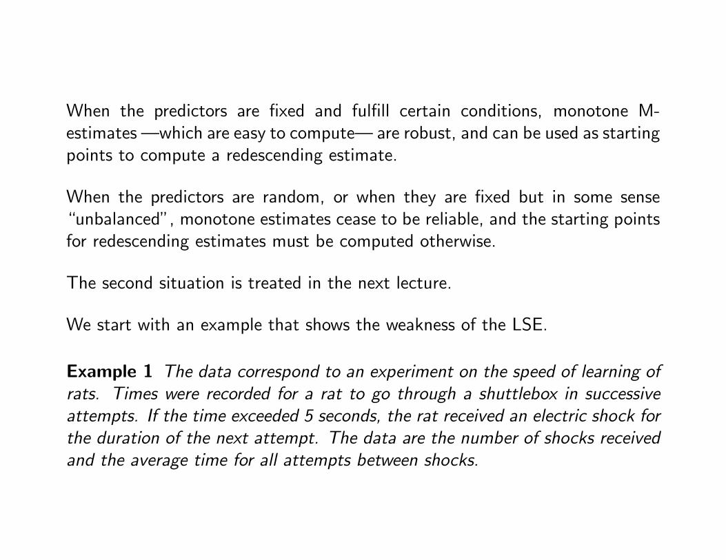
Example 1 The data correspond to an experiment on the speed of learning ofrats. Times were recorded for a rat to go through a shuttlebox in successiveattempts. If the time exceeded 5 seconds, the rat received an electric shock forthe duration of the next attempt. The data are the number of shocks receivedand the average time for all attempts between shocks.

number of shocks

aver

age 

time

0 5 10 15

24

68

1012

14

12

4

LS

LS ­

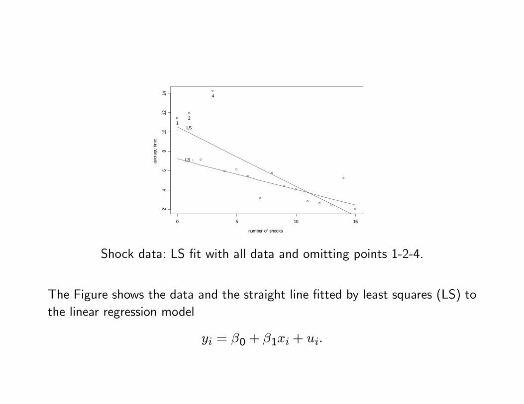
Shock data: LS �t with all data and omitting points 1-2-4.

The Figure shows the data and the straight line �tted by least squares (LS) tothe linear regression model

yi = �0 + �1xi + ui:

The relationship between the variables is seen to be roughly linear except forthe three upper left points.

The LS line does not �t the bulk of the data, being a compromise betweenthose three points and the rest.

The LS �t computed without using the three points gives a better representationof the majority of the data, while pointing out the exceptional character ofpoints 1-2-4.

We aim at developing procedures that give a good �t to the bulk of the datawithout being perturbed by a small proportion of outliers.

The Table gives the estimated parameters for LS with the complete data andwith the three atypical points deleted, and also for two robust estimates (L1and bisquare) to be de�ned later.

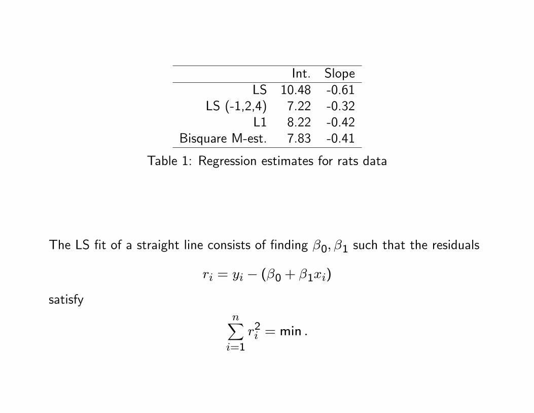
Int. SlopeLS 10.48 -0.61

LS (-1,2,4) 7.22 -0.32L1 8.22 -0.42

Bisquare M-est. 7.83 -0.41

Table 1: Regression estimates for rats data

The LS �t of a straight line consists of �nding �0; �1 such that the residuals

ri = yi � (�0 + �1xi)

satisfynXi=1

r2i = min :

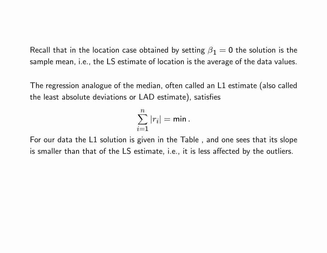
Recall that in the location case obtained by setting �1 = 0 the solution is thesample mean, i.e., the LS estimate of location is the average of the data values.

The regression analogue of the median, often called an L1 estimate (also calledthe least absolute deviations or LAD estimate), satis�es

nXi=1

jrij = min :

For our data the L1 solution is given in the Table , and one sees that its slopeis smaller than that of the LS estimate, i.e., it is less a¤ected by the outliers.

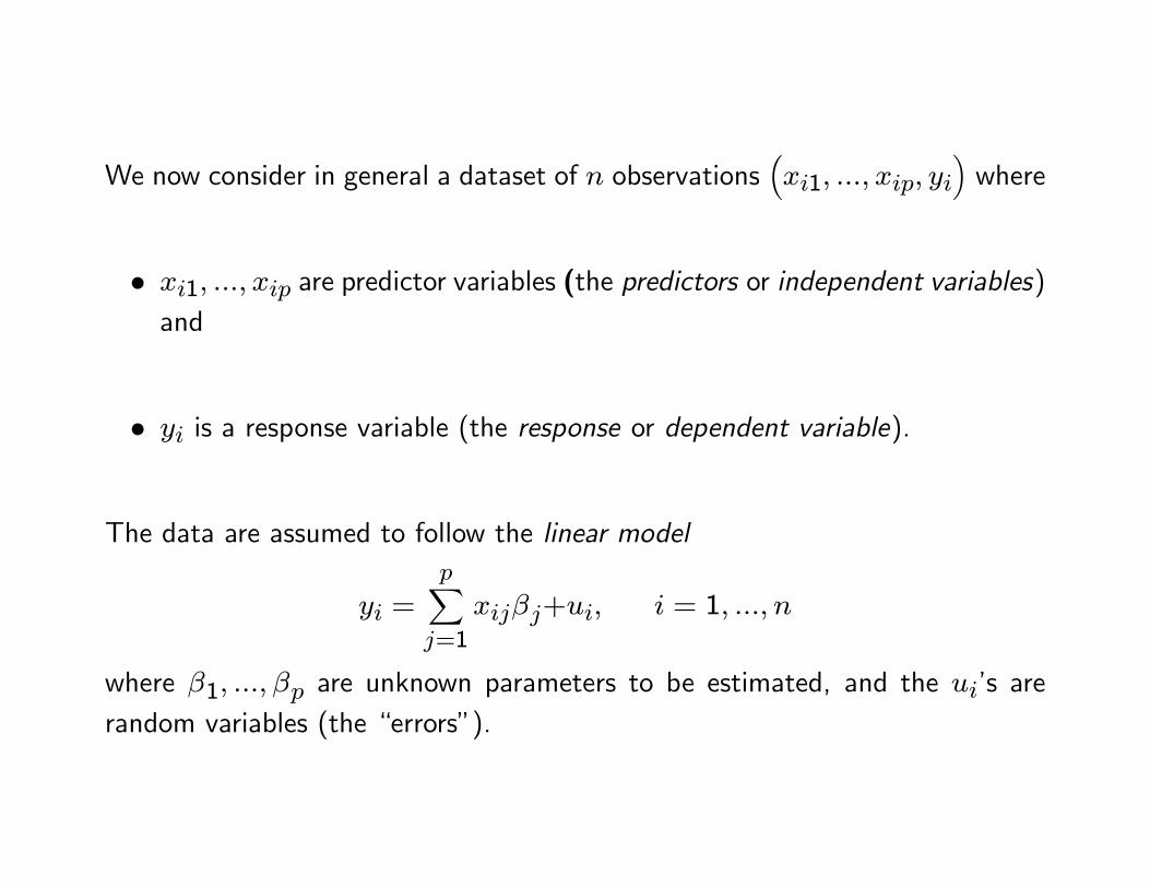
We now consider in general a dataset of n observations�xi1; :::; xip; yi

�where

� xi1; :::; xip are predictor variables (the predictors or independent variables)and

� yi is a response variable (the response or dependent variable).

The data are assumed to follow the linear model

yi =pXj=1

xij�j+ui; i = 1; :::; n

where �1; :::; �p are unknown parameters to be estimated, and the ui�s arerandom variables (the �errors�).

In a designed experiment, the xij�s are nonrandom (or �xed), i.e., determinedbefore the experiment.

When the data is observational the xij are random variables.

We sometimes have also mixed situations with both �xed and random predictors(Analysis of Covariance models).

Putting

xi = (xi1; :::; xip)0; � =

��1; :::; �p

�0;

the model can be more compactly written as

yi = x0i�+ui

where x0 is the transpose of x.

When the model has a constant term, the �rst coordinate of each xi is 1 andthe model may be written as

yi = �0 + x0i�1+ui

where xi and �1 are in Rp�1 and

xi =

1xi

!; � =

�0�1

!:

Here �0 is called the intercept and the elements of �1 are the slopes.

Call X the n � p-matrix with elements xij and let y and u the vectors withelements yi and ui respectively (i = 1; :::; n).

Then the linear model may be written

y = X� + u:

The �tted values byi and the residuals ri corresponding to a vector � are de�nedrespectively as

byi(�) = x0i� and ri(�)=yi � byi(�):The dependence of the �tted values and residuals on � will be dropped whenthis does not cause confusion.

We shall discuss regression M-estimates b� de�ned as solutions of equations ofthe form

nXi=1

�

ri(b�)b�!= min :

Here � is a �-function and b� is an auxiliary scale estimate that is required tomake b� scale equivariant.

The LSE and the L1 estimate correspond respectively to

�(t) = t2 and �(t) = jtj :

In these two cases b� becomes a constant factor and therefore neither the LSnor the L1 estimates require a scale estimate.

In a designed experiment, the predictors xij are �xed.

An important special case of �xed predictors is when they represent categoricalpredictors with values of either 0 or 1.

The simplest situation is the comparison of several treatments, usually called aone-way analysis of variance (or �one-way ANOVA�).

Here we have p samples yik (i = 1; :::; nk; k = 1; :::; p) and the model

yik = �k + uik

where the uik�s are i.i.d.

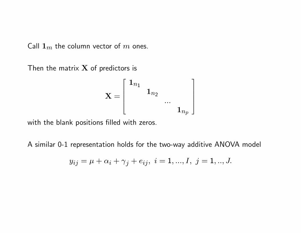
Call 1m the column vector of m ones.

Then the matrix X of predictors is

X =

266641n1

1n2:::

1np

37775with the blank positions �lled with zeros.

A similar 0-1 representation holds for the two-way additive ANOVA model

yij = �+ �i + j + eij; i = 1; :::; I; j = 1; ::; J:

2 Review of the least squares method

The method of least squares was proposed in 1805 by Legendre (for a fascinatingaccount, see (Stigler, 1986).

The main reason for its immediate and lasting success was that it was the onlymethod of estimation that could be e¤ectively computed before the advent ofelectronic computers.

The LS estimate of � is the b� such thatnXi=1

r2i (b�) = min :

Di¤erentiating with respect to � yields

nXi=1

ri(b�)xi = 0;

which is equivalent to the linear equations

X0Xb� = X0y;The above equations are usually called the �normal equations�.

If the model contains a constant term, it follows that the residuals have zeroaverage.

The matrix of predictors X is said to have full rank if its columns are linearlyindependent.

This is equivalent to

Xa 6= 0 8 a 6= 0

and also equivalent to the nonsingularity of X0X:

If X has full rank then the solution is unique and is given by

b�LS = b�LS(X;y) = �X0X��1X0y:If the model contains a constant term, then the �rst column of X is identicallyone, and the full rank condition implies that no other column is constant.

If X is not of full rank, for example in two-way ANOVA designs, then we havewhat is called collinearity.

When there is collinearity the parameters are not identi�able in the sense thatthere exist �1 6= �2 such that X�1 = X�2:

Collinearity implies that the normal equations have in�nite solutions, all yieldingthe same �tted values and hence the same residuals.

The LS estimate satis�es

b�LS(X;y +X ) =b�LS(X;y) + for all 2Rp

b�LS(X;�y) =�b�LS(X;y) for all � 2 R

and for all nonsingular p� p-matrices A

b�LS(XA;y) = A�1 b�LS(X;y):

These properties are called respectively regression, scale and a¢ ne equivariance.

These are desirable properties, since they allow us to know how the estimatechanges under these transformations of the data.

(But they are not a dogma: equivariance may be sacri�ced to gain predic-tive accuracy, as with Ridge Regression and Least Angle Regression for nearlycollinear data!).

Assume now that the ui�s are i.i.d. with

Eui = 0 and Var(ui) = �2

and that X is �xed, i.e., nonrandom, and of full rank.

Under the linear model with X of full rank b�LS is unbiased and its mean andcovariance matrix are given by

Eb�LS = �; Var(b�LS) = �2�X0X

��1where henceforth Var(y) will denote the covariance matrix of the randomvector y.

If Eui 6= 0; then b�LS will be biased.However if the model contains an intercept, the bias will only a¤ect the interceptand not the slopes.

Let p� be the rank of X:

Then an unbiased estimate of �2 is well de�ned by

s2 =1

n� p�

nXi=1

r2i :

whether or not X is of full rank.

If the ui�s are normal and X is of full rank, then b�LS is multivariate normalb�LS � Np(�; �2 �X0X��1);

where Np(�;�) denotes the p-variate normal distribution with mean vector �and covariance matrix �:

If the ui�s are not normal but have a �nite variance, then it can be shown usingthe Central Limit Theorem that for large nb�LS is approximately normal,provided that a so-called �Lindeberg condition� holds, which loosely speakingmeans that

none of the xi is �much larger� than the rest.

Let now be a linear combination of the parameters: = �0a with a aconstant vector.

Then the natural estimate of is b = b�0a; which is N( ; �2 ) with�2 = �2a0

�X0X

��1a:

An unbiased estimate of �2 is

b�2 = s2a0�X0X

��1a:

Con�dence intervals and tests for may be obtained from the fact that undernormality the �t statistic�

T =b � b�

has a t distribution with n� p� degrees of freedom, where p� = rank(X):

3 Classical methods for outlier detection

The most popular way to deal with regression outliers is to use LS and try to�nd the in�uential observations.

After they are identi�ed, some decision must be taken such as modifying ordeleting them and applying LS to the modi�ed data.

Many numerical and/or graphical procedures called regression diagnostics areavailable for detecting in�uential observations based on an initial LS �t.

The simplest are graphical:

� the normal quantile-quantile (QQ) plot of residuals (it should be approxi-mately linear)

� the plot of residuals vs. �tted values (it should show no structure).

The in�uence of one observation zi = (xi; yi) on the LS estimate dependsboth on yi being too large or too small compared to y�s from similar x�s andon how �large�xi is, i.e., how much leverage xi has.

Most popular diagnostics for measuring the in�uence of zi = (xi; yi) are basedon comparing the LS estimate based on the full data with LS based on omittingzi:

Call b� and b�(i) the LS estimates based on the full data and on the data withoutzi, and let by = Xb�; by(i) = Xb�(i)where ri = ri(

b�):

Note that if p� < p; then b�(i) is not unique, but by(i) is unique.Then the Cook distance of zi is

Di =1

p�s2

by(i) � by 2where p� = rank (X) and b� is the residual standard deviation estimate

s2 =1

n� p�

nXi=1

r2i :

Call H the matrix of the orthogonal projection on the image of X; that is, onthe subspace fX� : � 2Rpg :

The matrixH is the so-called �hat matrix�and its diagonal elements h1; :::; hnare the leverages of x1; :::;xn:

If p� = p; then H ful�lls

H = X�X0X

��1X0 and hi = x

0i

�X0X

��1xi:

The his satisfynXi=1

hi = p�; hi 2 [0; 1] :

It can be shown that the Cook distance is easily computed in terms of the hi :

Di =r2is2

hi

p� (1� hi)2:

While Di can detect outliers in simple situations, it fails for more complexcon�gurations and may even fail to recognize a single outlier.

The reason is that ri; hi and s may be largely in�uenced by the outlier.

It is safer to use statistics based on the �leave one out�approach, as follows.

The �leave one out� residual r(i) = yi � b�0(i)xi is known to be expressible asr(i) =

ri1� hi

:

and it is shown that

Var(r(i)) =�2

1� hi:

An estimate of �2 which is free of the in�uence of xi is the quantity s2(i) that

is de�ned like s2; but deleting the i-th observation from the sample.

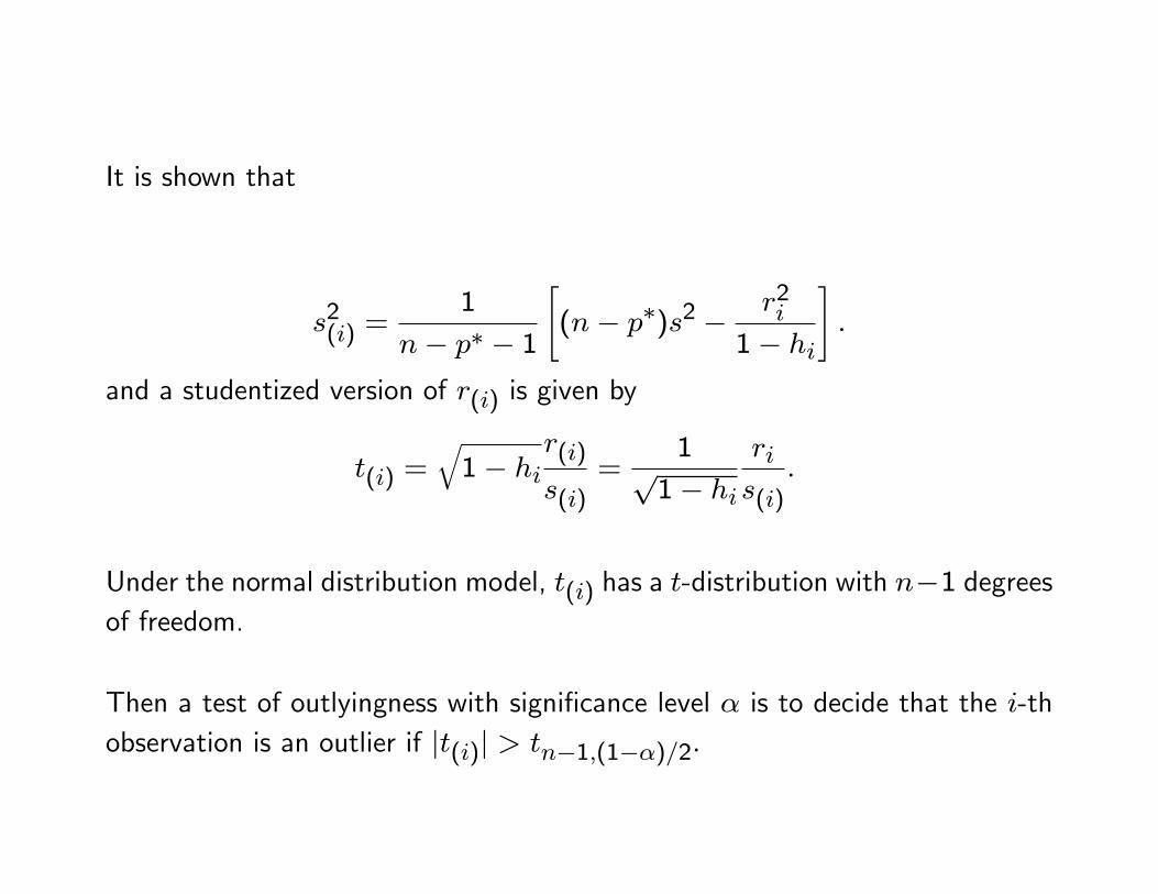
It is shown that

s2(i) =1

n� p� � 1

"(n� p�)s2 �

r2i1� hi

#:

and a studentized version of r(i) is given by

t(i) =q1� hi

r(i)

s(i)=

1p1� hi

ris(i)

:

Under the normal distribution model, t(i) has a t-distribution with n�1 degreesof freedom.

Then a test of outlyingness with signi�cance level � is to decide that the i-thobservation is an outlier if jt(i)j > tn�1;(1��)=2:

A graphical analysis is provided by the normal Q-Q plot of the t(i).

While the above "complete" leave-one-out approach ensures the detection of anisolated outlier, it can still be fooled by the combined action of several outliers,an e¤ect that is called masking.

Example 2 The data (Sche¤é 1959, p. 138) are the yield of grain for eightvarieties of oats in �ve replications of a randomized-block experiment.

The LS residuals have no noticeable structure, and the usual F-tests for rowand column e¤ects have highly signi�cant p-values of 0.00002 and 0.001, re-spectively.

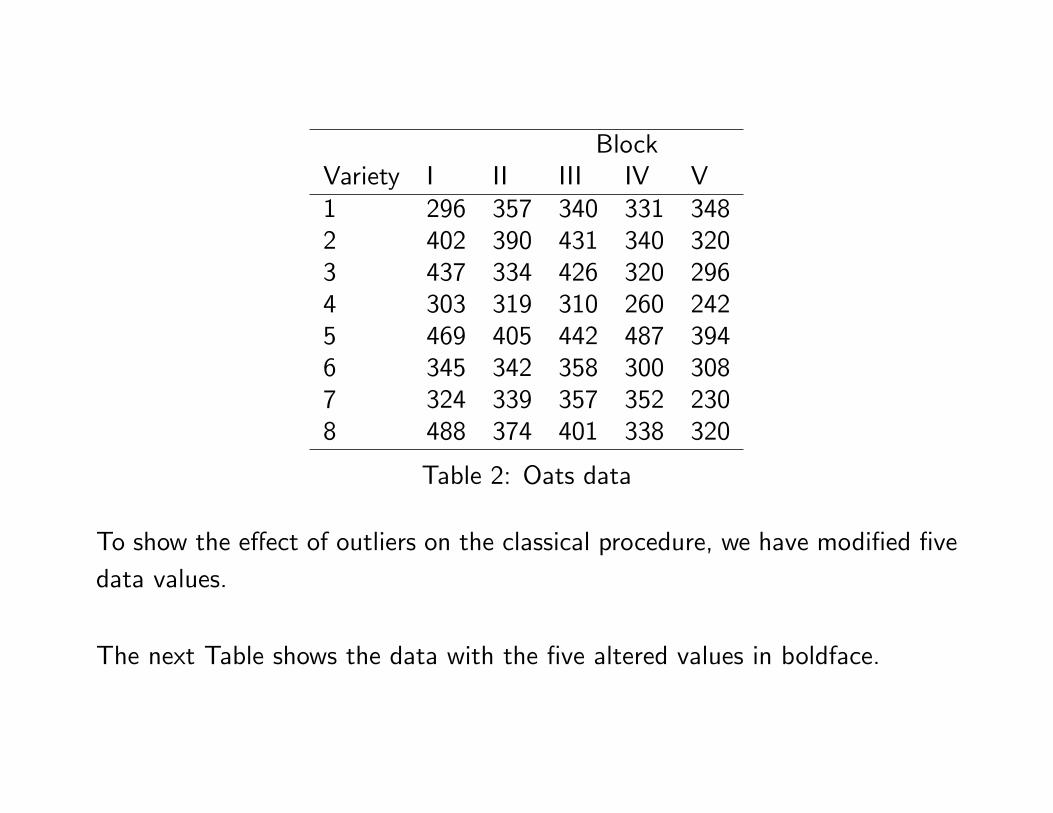
BlockVariety I II III IV V1 296 357 340 331 3482 402 390 431 340 3203 437 334 426 320 2964 303 319 310 260 2425 469 405 442 487 3946 345 342 358 300 3087 324 339 357 352 2308 488 374 401 338 320

Table 2: Oats data

To show the e¤ect of outliers on the classical procedure, we have modi�ed �vedata values.

The next Table shows the data with the �ve altered values in boldface.

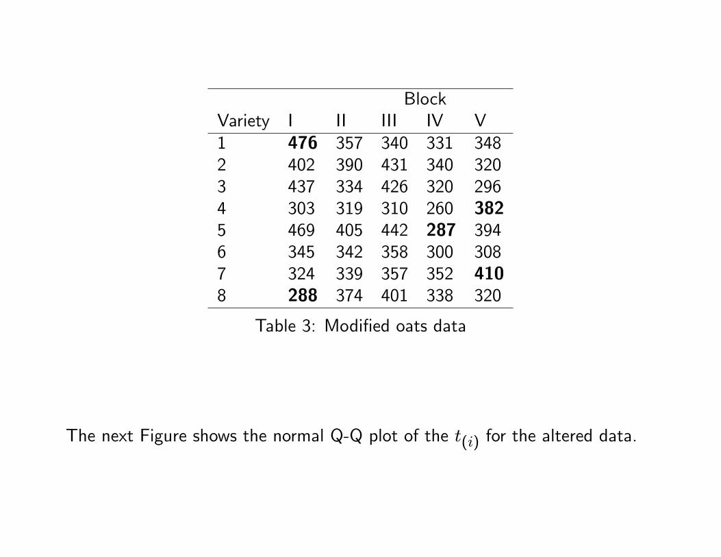
BlockVariety I II III IV V1 476 357 340 331 3482 402 390 431 340 3203 437 334 426 320 2964 303 319 310 260 3825 469 405 442 287 3946 345 342 358 300 3087 324 339 357 352 4108 288 374 401 338 320

Table 3: Modi�ed oats data

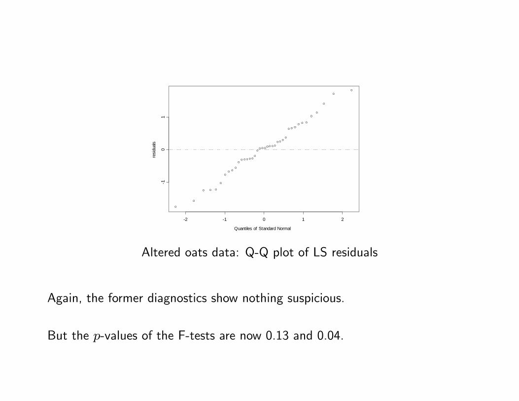
The next Figure shows the normal Q-Q plot of the t(i) for the altered data.

Quantiles of Standard Normal

resid

uals

­2 ­1 0 1 2

­10

1

Altered oats data: Q-Q plot of LS residuals

Again, the former diagnostics show nothing suspicious.

But the p-values of the F-tests are now 0.13 and 0.04.

The diagnostics have thus failed to point out a departure from the model, withserious consequences.

There exist much more sophisticated diagnostics in the literature.

All these procedures are fast, and are much better than naively �tting LSwithout further care.

But they are inferior to robust methods in several senses:

� they may fail in the presence of masking

� the distribution of the resulting estimate is unknown

� the variability may be underestimated

� once an outlier is found further ones may appear, and it is not clear whenone should stop.

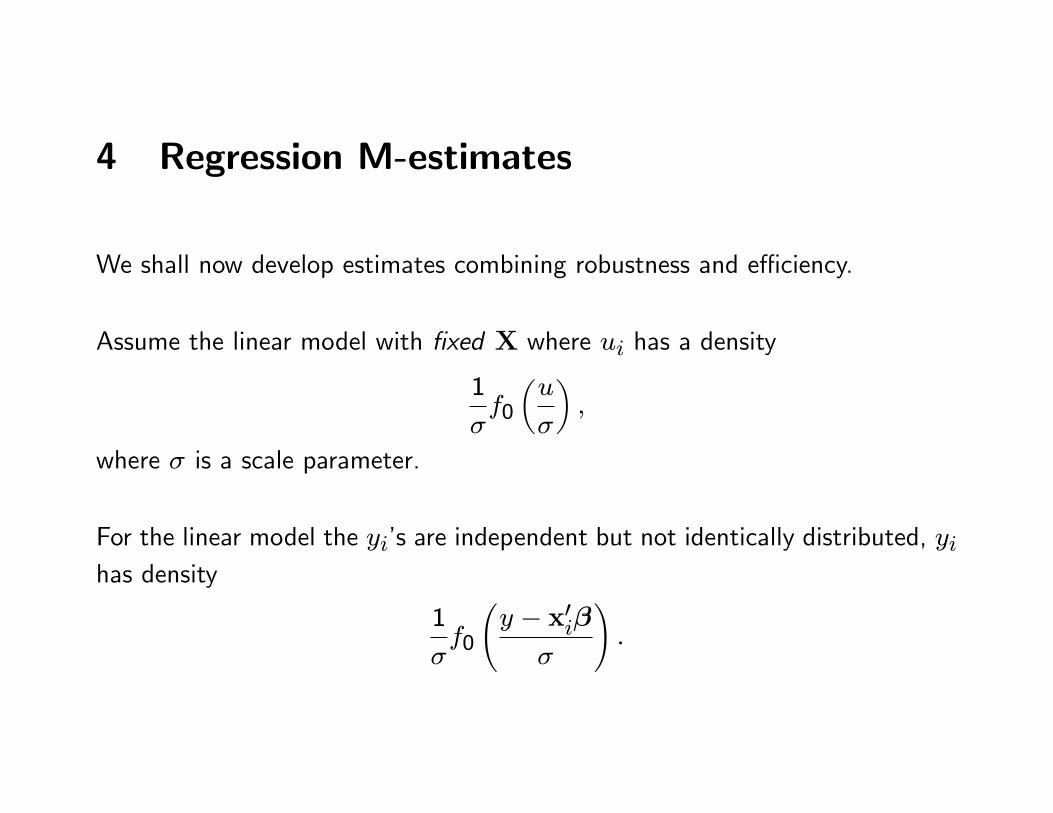
4 Regression M-estimates

We shall now develop estimates combining robustness and e¢ ciency.

Assume the linear model with �xed X where ui has a density

1

�f0

�u

�

�;

where � is a scale parameter.

For the linear model the yi�s are independent but not identically distributed, yihas density

1

�f0

y � x0i�

�

!:

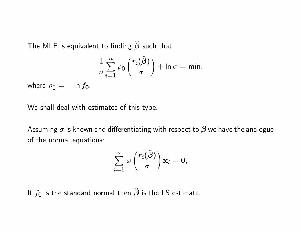
The MLE is equivalent to �nding b� such that1

n

nXi=1

�0

ri(b�)�

!+ ln� = min;

where �0 = � ln f0.

We shall deal with estimates of this type.

Assuming � is known and di¤erentiating with respect to � we have the analogueof the normal equations:

nXi=1

ri(b�)�

!xi = 0;

If f0 is the standard normal then b� is the LS estimate.

If f0 is the double exponential density then b� satis�esnXi=1

���ri(b�)��� = minand b� is called an L1 estimate, which is the regression equivalent of the median.The L1 estimate was studied before LS (by Boscovich in 1757 and Laplace in1799).

Unlike LS there are in general no explicit expressions for an L1 estimate.

However there exist very fast algorithms to compute it.

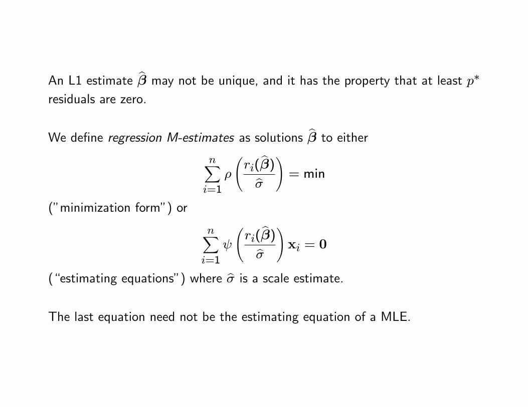
An L1 estimate b� may not be unique, and it has the property that at least p�residuals are zero.

We de�ne regression M-estimates as solutions b� to eithernXi=1

�

ri(b�)b�!= min

(�minimization form�) or

nXi=1

ri(b�)b�!xi = 0

(�estimating equations�) where b� is a scale estimate.The last equation need not be the estimating equation of a MLE.

In most situations considered here, b� is computed previously, but it can also becomputed simultaneously through a scale M-estimating equation.

It will henceforth be assumed that � and are respectively a �- and a -function in the sense of the De�nition.

The matrix X will be assumed to have full rank.

These estimates are regression, a¢ ne and scale equivariant

Solutions to the estimating equations with monotone (resp. redescending) are called monotone (resp. redescending) regression M-estimates.

The main advantage of monotone estimates is that all solutions of the estimat-ing equations are solutions of the minimization form.

Furthermore if is strictly increasing then the solution is unique.

We had seen that in the case of redescending location estimates, the estimatingequation may have �bad� roots.

This cannot happen with monotone estimates.

On the other hand, we have seen that redescending M-estimates of locationyield a better trade-o¤ between robustness and e¢ ciency,and the same can be shown to hold in the regression context.

Computing redescending estimates requires a starting point, and this will bethe main role of monotone estimates.

4.1 M-estimates with known scale

Assume the linear model with errors u such that

E �u

�

�= 0

which holds in particular if u is symmetric and odd.

Then under certain conditions on X; b� is consistent for � in the sense thatb� !p �

when n!1; and furthermore for large n

D(b�) � Np(�; v �X0X��1)

where v is the same as for location:

v = �2E (u=�)2�E 0 (u=�)

�2:Thus the approximate covariance matrix of an M-estimate di¤ers only by aconstant factor from that of the LS estimate.

Hence its e¢ ciency for normal u�s does not depend on X:

If we have a model with intercept and

E �u

�

�= 0

does not hold, then the intercept is asymptotically biased, but the slope esti-mates are none-the-less consistent :b�1 !p �1:

4.2 M-estimates with preliminary scale

For estimating location with an M-estimate, we estimated � using the MAD.

Here the equivalent procedure is to �rst compute the L1 �t and from it obtainthe analogue of the normalized MAD by taking the median of the nonnullabsolute residuals:

b� = 1

0:675Medi(jrij j ri 6= 0):

The reason for using only nonnull residuals is that since at least p residuals arenull, when p is large including all residuals could lead to underestimating �:

Recall that the L1 estimate does not require estimating a scale.

Write b� as b�(X;y): Then since the L1 estimate is regression, scale and a¢ neequivariant, it is easy to show that

b�(X;y +X ) = b�(X;y);b�(XA;y) = b�(X;y);b�(X;�y) = j�j b�(X;y)for all 2Rp; nonsingular A 2 Rp�p and � 2 R.

We say that b� is regression and a¢ ne invariant and scale equivariant.We then obtain a regression M-estimate by solving the optimization form orthe estimating equations with b� instead of �:

Then the properties of b� imply that b� is regression, a¢ ne and scale equivariant.Assume that b� !p �. Then for large n the distribution of b� is approximatelynormal with covariance matrix v

�X0X

�=1 where

v = �2E (u=�)2�E 0 (u=�)

�2i.e., that b� can be replaced by �.Thus the e¢ ciency of the estimate does not depend on X:

If the model contains an intercept the approximate distribution result holds forthe slopes without any requirement on ui.

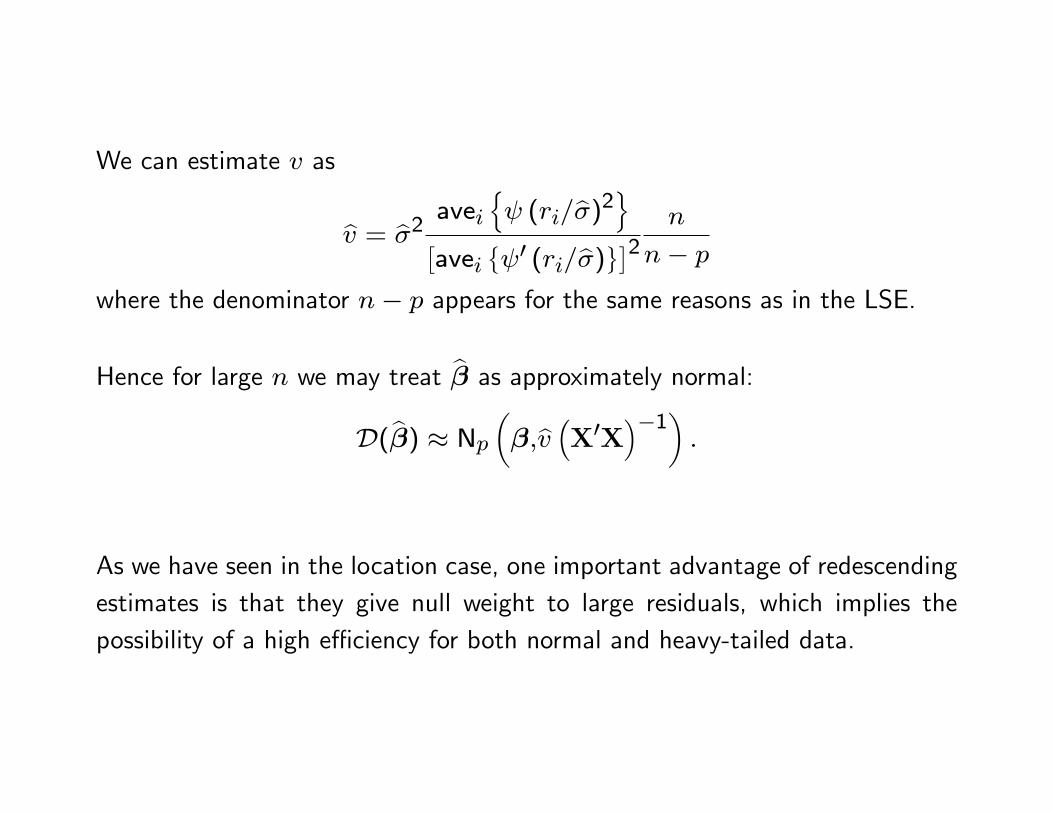
We can estimate v as

bv = b�2 avein (ri=b�)2o�

avei� 0 (ri=b�)�2

n

n� p

where the denominator n� p appears for the same reasons as in the LSE.

Hence for large n we may treat b� as approximately normal:D(b�) � Np ��;bv �X0X��1� :

As we have seen in the location case, one important advantage of redescendingestimates is that they give null weight to large residuals, which implies thepossibility of a high e¢ ciency for both normal and heavy-tailed data.

This is valid also for regression since the e¢ ciency depends only on v which isthe same as for location.

Therefore our recommended procedure is to use L1 as a basis for computing b�and as a starting point for the iterative computing of a bisquare M-estimate.

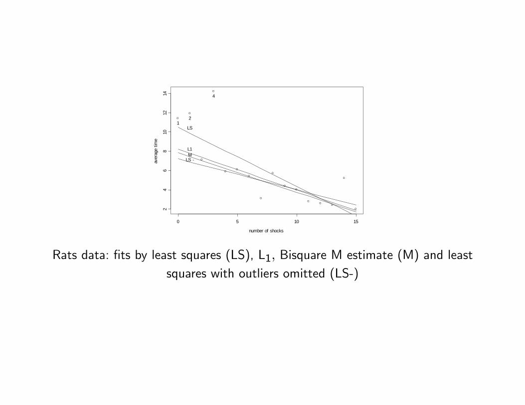
Example 1 (continuation) The Figure shows the �tted lines for the bisquareM-estimate with 0.85 e¢ ciency, the LS estimate using the full data, the LSestimate computed without the points labeled 1, 2, 4, and the L1 estimate.

The results are very similar to the LS estimate computed without the threeatypical points.

number of shocks

aver

age 

time

0 5 10 15

24

68

1012

14

12

4

LS

L1M

LS ­

Rats data: �ts by least squares (LS), L1; Bisquare M estimate (M) and leastsquares with outliers omitted (LS-)

The estimated standard deviations of the slope are 0.122 for LS and 0.050 forthe bisquare M-estimate, and the respective con�dence intervals with level 0.95are (-0.849, -0.371) and (-0.580, -0.384).

It is seen that the outliers in�ate the con�dence interval based on the LSestimate relative to that based on the bisquare M-estimate.

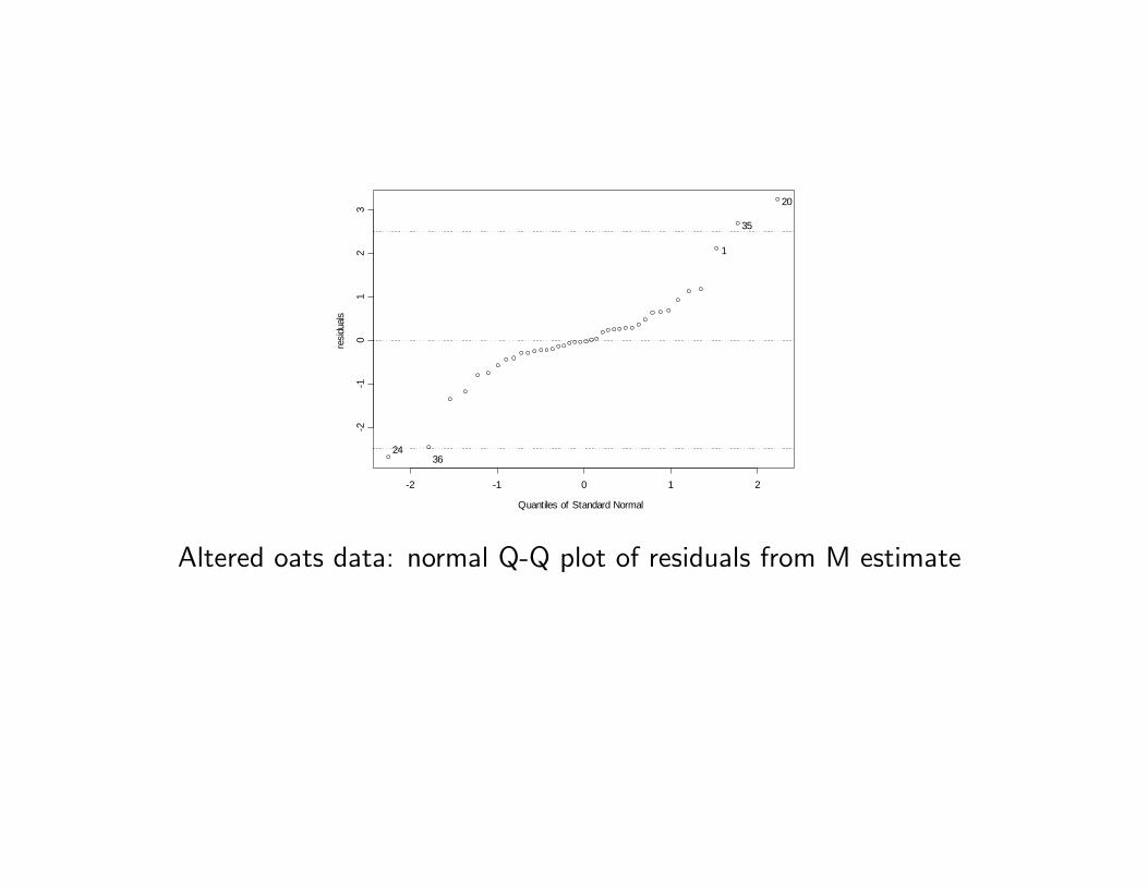
Example 2 (continuation) The Figure shows the residual Q-Q plot based onthe bisquare M-estimate, and it is seen that the �ve modi�ed values stand outfrom the rest.

Quantiles of Standard Normal

resid

uals

­2 ­1 0 1 2

­2­1

01

23

2436

1

35

20

Altered oats data: normal Q-Q plot of residuals from M estimate

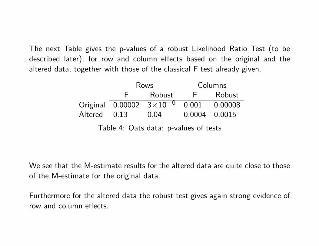
The next Table gives the p-values of a robust Likelihood Ratio Test (to bedescribed later), for row and column e¤ects based on the original and thealtered data, together with those of the classical F test already given.

Rows ColumnsF Robust F Robust

Original 0.00002 3�10�6 0.001 0.00008Altered 0.13 0.04 0.0004 0.0015

Table 4: Oats data: p-values of tests

We see that the M-estimate results for the altered data are quite close to thoseof the M-estimate for the original data.

Furthermore for the altered data the robust test gives again strong evidence ofrow and column e¤ects.

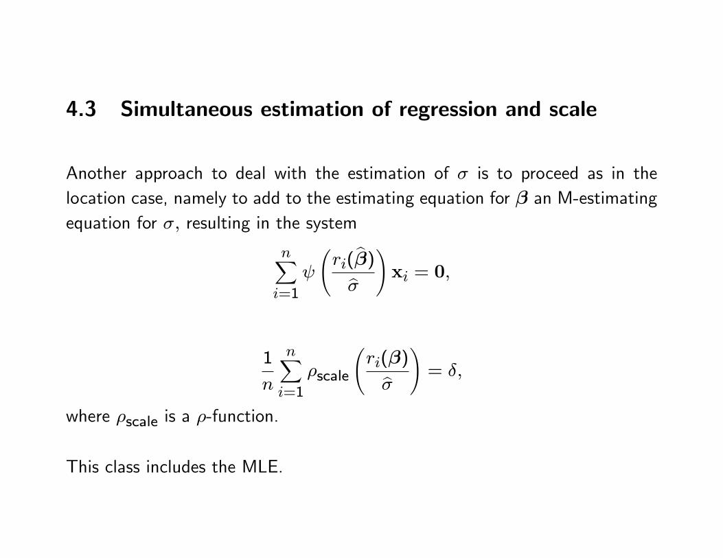
4.3 Simultaneous estimation of regression and scale

Another approach to deal with the estimation of � is to proceed as in thelocation case, namely to add to the estimating equation for � an M-estimatingequation for �; resulting in the system

nXi=1

ri(b�)b�!xi = 0;

1

n

nXi=1

�scale

ri(�)b�

!= �;

where �scale is a �-function.

This class includes the MLE.

Simultaneous estimates with monotonic are less robust than those of theformer section , but they will be used with redescending in another contextin the next lecture.

5 Numerical computing of monotone M-estimates

5.1 The L1 estimate

As was mentioned above, computing the L1 estimate requires sophisticatedalgorithms like the one due to Barrodale and Roberts (1973).

There are however some cases in which this estimate can be computed explicitly.For regression through the origin (yi = �xi + ui);

b� is a �weighted median�For one-way ANOVA it is immediate that the L1 estimates are the samplemedians b�k = Medi (yik) :And for two-way ANOVA with one observation per cell there is a simple methodcalled �median polish� (Tukey 1977).

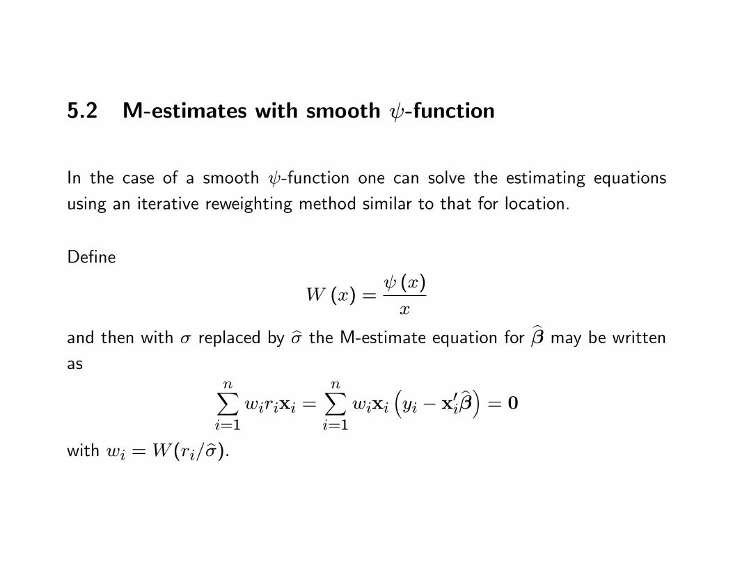
5.2 M-estimates with smooth -function

In the case of a smooth -function one can solve the estimating equationsusing an iterative reweighting method similar to that for location.

De�ne

W (x) = (x)

x

and then with � replaced by b� the M-estimate equation for b� may be writtenas

nXi=1

wirixi =nXi=1

wixi�yi � x0i b�� = 0

with wi =W (ri=b�):

These are �weighted normal equations�, and if the wi were known, the equa-tions could be solved by applying LS to the �weighted data�

pwiyi and

pwixi:

But the wi are not known and depend upon the data.

So the procedure, which depends on a tolerance parameter "; is as follows

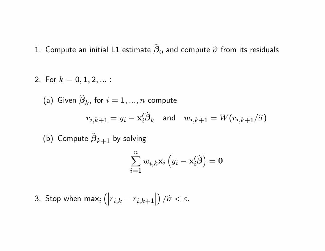
1. Compute an initial L1 estimate b�0 and compute b� from its residuals

2. For k = 0; 1; 2; ::: :

(a) Given b�k; for i = 1; :::; n computeri;k+1 = yi � x0i b�k and wi;k+1 =W (ri;k+1=b�)

(b) Compute b�k+1 by solvingnXi=1

wi;kxi�yi � x0i b�� = 0

3. Stop when maxi����ri;k � ri;k+1

���� =b� < ":

This algorithm converges if W (x) is nonincreasing for x > 0.

If is monotone, since the solution is essentially unique, the choice of thestarting point in�uences the number of iterations but not the �nal result.

This procedure is called �iteratively reweighted least squares� (IRWLS).

For simultaneous estimation of � and � the procedure is the same, except thatat each iteration b� is also updated at each step.

6 Breakdown point of monotone regression esti-

mates

Assume for simplicity X of full rank so that the estimates are well de�ned.

Since X is �xed only y can be changed, and this requires a modi�cation of thede�nition of the breakdown point.

The FBP for regression with �xed predictors is de�ned as

"� =m�

n;

with

m� = maxnm � 0 : b�(X;ym) bounded 8 ym 2 Ym

o:

where Ym is the set of n�vectors with at least n �m elements in commonwith y:

It is clear that the LS estimate has "� = 0:

Let k� = k�(X) be the maximum number of xi lying on the same subspace:

k�(X) =maxn#��0xi = 0

�: � 2Rp; � 6= 0

owhere a subspace of dimension zero is the set f0g.

In the case of simple straight-line regression k� is the maximum number ofrepeated xi�s.

We have always k� � p� 1:

If k� = p� 1 then X is said to be in general position.

In the case of a model with intercept, X is in general position i¤ no more thanp� 1 of the xi lie on a hyperplane.

It is shown that for all regression equivariant estimates

"� � "�max :=m�maxn

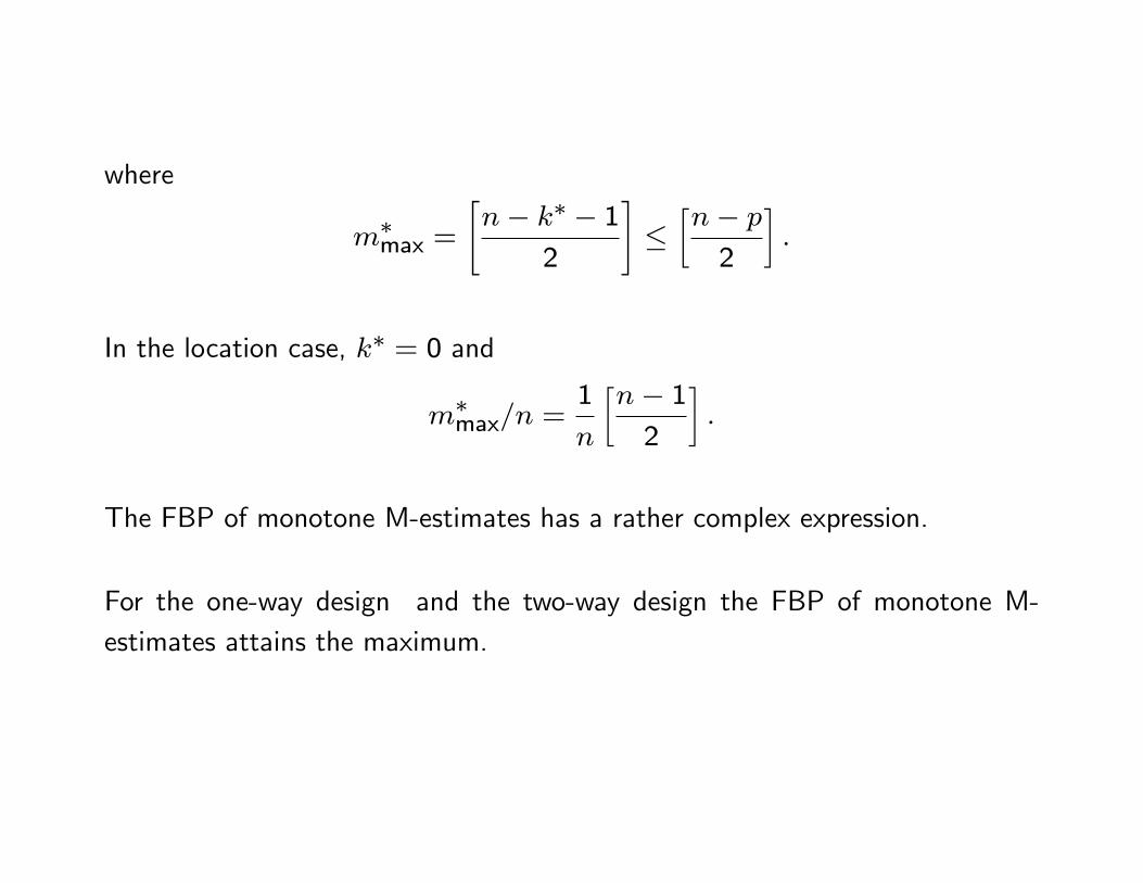
where

m�max =

"n� k� � 1

2

#��n� p

2

�:

In the location case, k� = 0 and

m�max=n =1

n

�n� 12

�:

The FBP of monotone M-estimates has a rather complex expression.

For the one-way design and the two-way design the FBP of monotone M-estimates attains the maximum.

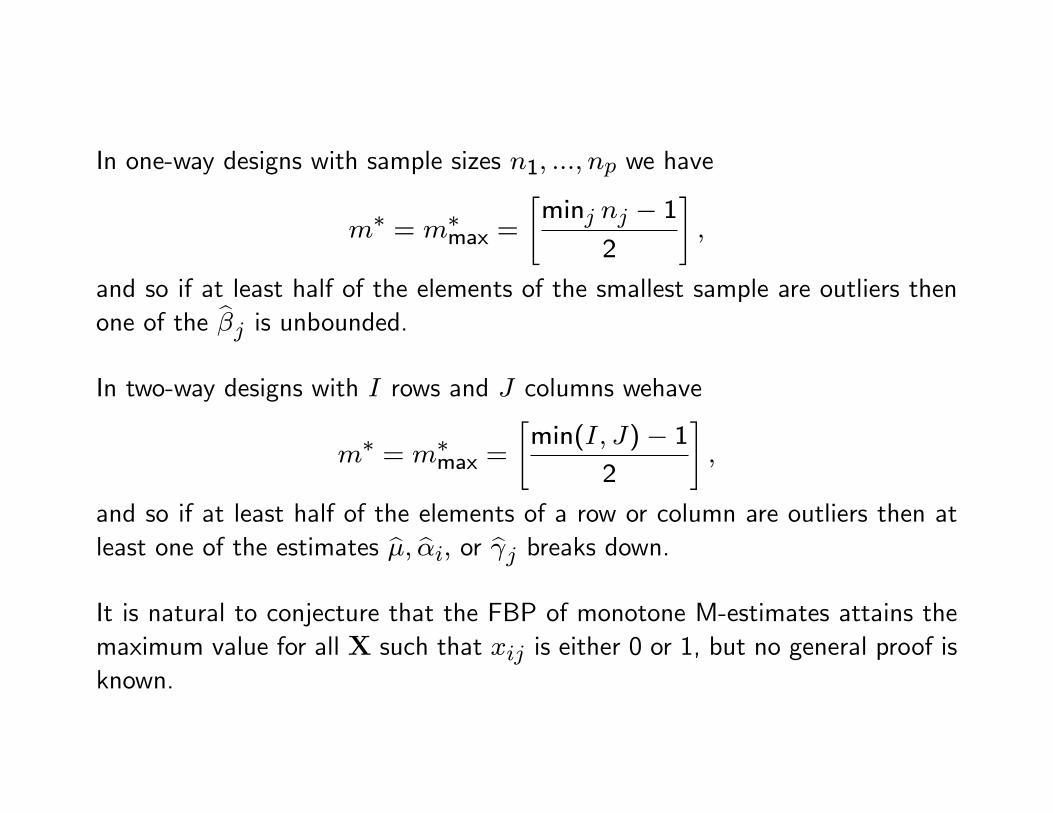
In one-way designs with sample sizes n1; :::; np we have

m� = m�max =

"minj nj � 1

2

#;

and so if at least half of the elements of the smallest sample are outliers thenone of the b�j is unbounded.In two-way designs with I rows and J columns wehave

m� = m�max =

"min(I; J)� 1

2

#;

and so if at least half of the elements of a row or column are outliers then atleast one of the estimates b�; b�i; or b j breaks down.It is natural to conjecture that the FBP of monotone M-estimates attains themaximum value for all X such that xij is either 0 or 1, but no general proof isknown.

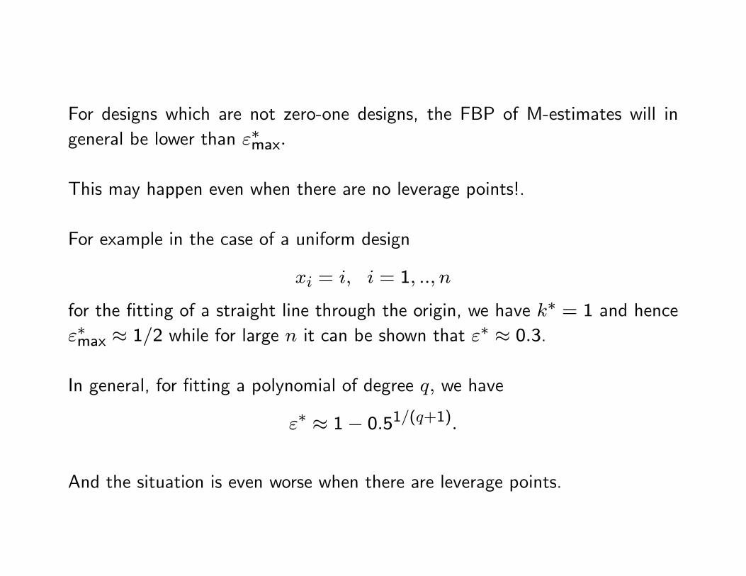
For designs which are not zero-one designs, the FBP of M-estimates will ingeneral be lower than "�max:

This may happen even when there are no leverage points!.

For example in the case of a uniform design

xi = i; i = 1; ::; n

for the �tting of a straight line through the origin, we have k� = 1 and hence"�max � 1=2 while for large n it can be shown that "� � 0:3.

In general, for �tting a polynomial of degree q; we have

"� � 1� 0:51=(q+1):

And the situation is even worse when there are leverage points.

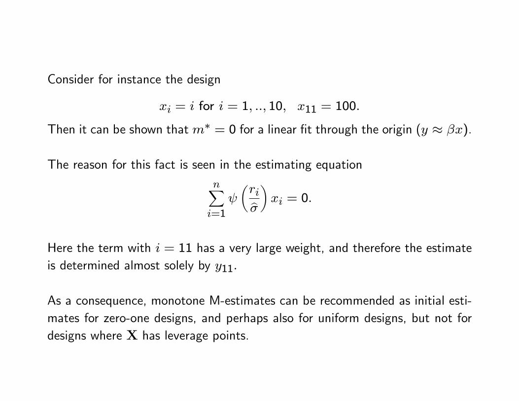
Consider for instance the design

xi = i for i = 1; ::; 10; x11 = 100:

Then it can be shown thatm� = 0 for a linear �t through the origin (y � �x).

The reason for this fact is seen in the estimating equation

nXi=1

�rib��xi = 0:

Here the term with i = 11 has a very large weight, and therefore the estimateis determined almost solely by y11:

As a consequence, monotone M-estimates can be recommended as initial esti-mates for zero-one designs, and perhaps also for uniform designs, but not fordesigns where X has leverage points.

The case of random X will be treated in the next lecture.

The techniques discussed there will be also applicable to �xed designs withleverage points.

7 Robust tests for linear hypothesis

Regression M-estimates can be used to obtain robust approximate con�denceintervals and tests for a single linear combination of the parameters.

For general linear hypothesis, a robust version of the Likelihood Ratio Test hasbeen developed.

Its derivation is like that of the F-test but with a �-function of the residualsinstead of their squares.

Details are complex and are omitted for reasons of time.