linear relations among double zeta values in positive...

LINEAR RELATIONS AMONG DOUBLE ZETA VALUES INPOSITIVE CHARACTERISTIC

CHIEH-YU CHANG

Dedicated to the memory of my father

Abstract. For each integer n ≥ 2, we study linear relations among weight n double zetavalues and the nth power of the Carlitz period over the rational function field Fq(θ). Weshow that all the Fq(θ)-linear relations are induced from the Fq[t]-linear relations amongcertain explicitly constructed special points in the nth tensor power of the Carlitz module.We then establish a principle of Siegel’s lemma for computing and determining the Fq[t]-linear relations mentioned above, and thus obtain an effective criterion for computing thedimension of weight n double zeta values space.

1. Introduction

1.1. Classical theory. Classical multiple zeta values (abbreviated as MZV’s) are definedby the series: for s = (s1, . . . , sr) ∈Nr with s1 ≥ 2,

ζ(s) := ∑n1>···>nr≥1

1ns1

1 · · · nsrr∈ R×.

Here wt(s) := ∑ri=1 si is called the weight and r is called the depth of the presenta-

tion ζA(s). MZV’s have many connections with various research topics. For example,see [Z93, Z94, Cart02, Andre04, B12, Zh16].

Let Z0 := Q, Z1 := 0 and Zn be the Q-vector space spanned by the weight n MZV’sfor integers n ≥ 2. Putting Z := ∑n≥0 Zn. It is well known that ZmZn ⊆ Zm+n, and so Zhas a Q-algebra structure. The Goncharov’s direct sum conjecture [Gon97] asserts thatZ is a graded algebra (graded by weights). Therefore, understanding the Q-algebraicrelations among MZV’s boils down to understanding the Q-linear relations among thesame weight MZV’s. However, to date computing the dimension of Zn for each n is outof reach. Note that Zagier’s dimension conjecture predicts that dn := dimQ Zn satisfiesthe recursive relation

dn = dn−2 + dn−3 for n ≥ 3,

and one knows by Goncharov and Terasoma that dimQ Zn ≤ dn for each n (see [Te02,DG05]).

Date: July 6, 2016.2010 Mathematics Subject Classification. Primary 11R58, 11J93; Secondary 11G09, 11M32, 11M38.Key words and phrases. Double zeta values, t-motives, Carlitz tensor powers, periods, logarithms, Siegel’s

lemma.The author was partially supported by a Golden-Jade fellowship of the Kenda Foundation and MOST

Grant 102-2115-M-007-013-MY5. He thanks NCTS for offering a center scientist position, which is veryhelpful to research.

1

2 CHIEH-YU CHANG

Now, we focus on depth two MZV’s, which are called double zeta values. It is anatural question to ask how to compute the dimension of the Q-vector space

DZn := SpanQ

(2π√−1)n, ζ(2, n− 2), ζ(3, n− 3), · · · , ζ(n− 1, 1)

for n ≥ 3. This is still a very difficult problem in the classical theory as dimQ DZn is onlyknown for n = 3, 4. Zagier (cf. [Z94]) gave a conjectural formula for dn in terms of thedimension of weight n cusp forms.

Conjecture 1.1.1. (Zagier) For n ≥ 3, we put

sn :=

n2 − 1− dimC Sn(SL2(Z)) if n is even,n+1

2 if n is odd,

where Sn(SL2(Z)) is space of weight n cusp forms for SL2(Z). Then we have

dimQ DZn = sn.

The best known result toward this conjecture is due to Gangl, Kaneko and Zagier [GKZ06],who showed that dimQ DZn ≤ sn for each n ≥ 3. One of their approaches is to introduceand study the double Eisenstein series to explain the relation between double zeta val-ues and cusp forms for SL2(Z). The main result of this paper is to establish an effectivecriterion for computing the analogue of dimQ DZn in the positive characteristic functionfield setting.

1.2. The main result. Let A := Fq[θ] be the polynomial ring in the variable θ over thefinite field Fq of q elements with characteristic p, and k be its quotient field. Denote by∞ the infinite place of k. Let k∞ := Fq((

1θ )) be the ∞-adic completion of k, and k∞ be a

fixed algebraic closure of k∞. Denote by C∞ the ∞-adic completion of k∞. Finally, we letA+ be the set of all monic polynomials in A. We then have the following comparisons:

A+ ↔N, A↔ Z, k↔ Q, k∞ ↔ R, C∞ ↔ C.

For any r-tuple of positive integers s = (s1, . . . , sr) ∈ Nr, Thakur [T04] introduced themultiple series

ζA(s) := ∑1

as11 · · · a

srr∈ k∞,

where the sum is taken over r-tuples (a1, . . . , ar) ∈ Ar+ satisfying the strict inequalities

degθ a1 > · · · > degθ ar. In analogy with the classical MZV’s, r is called the depthand wt(s) := s1 + · · ·+ sr is called the weight of the presentation ζA(s). These specialvalues ζA(s) are called multizeta values (abbreviated as MZV’s too) and each of them isnon-vanishing by [T09a]. Moreover, these MZV’s have a t-motivic interpretation in thesense that they occur as periods of certain mixed Carlitz-Tate t-motives by the work ofAnderson and Thakur [AT09].

In [T10], Thakur showed that the product of two MZV’s can be expressed as an Fp-linear combination of some MZV’s with the same weight, which is regarded as a kind ofshuffle product relation (cf. (1.2.2)), and so the Fp-vector space spanned by MZV’s has aring structure. Further, an analogue of Goncharov’s direct sum conjecture was shown bythe author [C14], that the k-algebra generated by all MZV’s is a graded algebra (gradedby weights). In other words, all k-linear relations among MZV’s are generated by thosek-linear relations among the same weight MZV’s.

LINEAR RELATIONS AMONG DOUBLE ZETA VALUES 3

In the classical theory of MZV’s, (regularized) double shuffle relations give rise to richQ-linear relations among the same weight MZV’s (see [IKZ06]). Unlike the classical sit-uation, there is no natural total order on A+ and so far a nice analogue of the iteratedintegral expression for MZV’s is not developed yet. To date there is no different expres-sion for the product of two MZV’s other than Thakur’s relation mentioned above, andhence we do not have the analogue of double shuffle relations to produce k-linear rela-tions among MZV’s naturally. In his Ph.D. thesis, Todd [To15] tried to produce k-linearrelations among the same weight MZV’s using power sums and used lattice reductionmethods to give a conjecture on the dimensions in question.

Let π be a fixed fundamental period of the Carlitz Fq[t]-module C, which plays theanalogous role of 2π

√−1, and let C⊗n be the nth tensor power of the Carlitz module

C for a positive integer n (see §§ 2.2 for the definitions). The main result of this papergives a new point of view to completely determine the k-linear relations among weightn double zeta values together with πn. It is stated as follows and its proof is given inCorollary 5.2.1 and Theorem 6.1.1.

Theorem 1.2.1. Let n ≥ 2 be a positive integer. Put

V :=(s1, s2) ∈N2; s1 + s2 = n and (q− 1)|s2

.

(1) For each s ∈ V , we explicitly construct a special point Ξs ∈ C⊗n(A) so that

dimk Spank πn, ζA(1, n− 1), ζA(2, n− 2), · · · , ζA(n− 1, 1)

= n− bn−1q−1 c+ rankFq[t] SpanFq[t] Ξss∈V .

(2) We establish an effective algorithm for computing the rank

rankFq[t] SpanFq[t] Ξss∈V .

In other words, we relate the k-linear relations among double zeta values to the Fq[t]-linear relations among the special points Ξss∈V , and which can be effectively com-puted and determined.

We mention that although Todd [To15] provided some ways of producing k-linearrelations among the same weight MZV’s, it is not clear how to derive k-linear relationsamong weight n double zeta values together with πn from Todd’s relation. When thegiven weight n ≥ 2 is A-even, ie., (q− 1)|n (as q− 1 is the cardinality of the unit groupA×), one can use the following formula to produce linear relations. For two positiveA-even integers r and s with r + s = n, one has

(1.2.2)

ζA(r)ζA(s) = ζA(r, s) + ζA(s, r) + ζA(r + s)

+ ∑i+j=n(q−1)|j

[(−1)s−1

(j− 1s− 1

)+ (−1)r−1

(j− 1r− 1

)]ζA(i, j)

(see [T10] for the existence of such relations and [Chen15] for the explicit formula). Bywork of Carlitz [Ca35], we know that

ζA(r)/πr ∈ k, ζA(s)/πs ∈ k, ζA(n)/πn ∈ k,

and so (1.2.2) gives rise to a nontrivial linear relation among πn and weight n doublezeta values. As all the coefficients of the double zeta values are in Fp, Thakur call itan “Fp-linear reation”. Our effective algorithm based on Theorem 1.2.1 is able to find

4 CHIEH-YU CHANG

all the independent k-linear relations in question. As observed by Thakur [T09b], thoseFp-linear relations produced by (1.2.2) can not generate all the k-linear relations, and ourcomputational data can capture the difference precisely. We refer the reader to the endof this paper.

We mention that there is a difference between Conjecture 1.1.1 and our results, andrefer the reader to Remark 3.1.12 about the detailed comparison. We further mentionthat in [Chen16], Drinfeld double Eisenstein series are introduced. Since double zetavalues occur as the constant terms of Drinfeld double Eisenstein series, one naturallyexpects that Drinfeld cusps forms [Go80, Ge88] can have connections with double zetavalues if they can be shown to be a subspace of the space of Drinfeld double Eisensteinseries (cf. [GKZ06]).

1.3. Methods of proof. Let notation and hypothesis be given as in Theorem 1.2.1. Weoutline the major steps in the proof of Theorem 1.2.1.

(I) A necessary condition. We show that all the k-linear relations among the set

πn ∪ ζA(1, n− 1), . . . , ζA(n− 1, 1)are those coming from the k-linear relations among πn ∪ ζA(s)s∈V , and sowe are reduced to studying the k-linear relations among πn ∪ ζA(s)s∈V . Thisresult is Corollary 3.1.10.

(II) Logarithmic interpretion. Let r ≥ 2. For any s = (s1, . . . , sr) ∈Nr with ζA(s2, . . . , sr)Eulerian, ie.,

ζA(s2, . . . , sr)/πs2+···+sr ∈ k,

we relate ζA(s) to the last coordinate of the logarithm of C⊗(s1+···+sr) at an explicitintegral point. This result is Theorem 4.1.1.

(III) The identity. Using the results in (I) and (II), we establish the equality in Theo-rem 1.2.1 (1) by appealing to Yu’s transcendence theory [Yu91] for the last coor-dinate of the logarithm of C⊗n at algebraic points. This result is Corollary 5.2.1.

(IV) A Siegel’s Lemma. We establish a principle of Siegel’s lemma for integral pointsin C⊗n to achieve Theorem 1.2.1 (2). This result is Theorem 6.1.1.

The four steps laid out above give an approach toward producing k-linear relationsamong the same weight MZV’s of arbitrary depths. Actually, for weight n ≥ 2 combiningthe ideas of (II), (III) and (IV) above one determine all the k-linear relations among theset

ζA(n) ∪ ζA(s); s ∈ En ,where En is the set consisting of all s ∈ Nr with r ≥ 2 and wt(s) = n satisfying thatζA(s

′) is Eulerian, where s′ = (s2, . . . , sr) for s = (s1, . . . , sr). This result is Corollary 5.1.3together with Theorem 6.1.1. In [CPY14] an effective criterion for Eulerian MZV’s isestablished, and conjecturally one can describe the set En precisely (see [CPY14, § 6.2]).We note that assuming Todd’s dimension conjecture [To15], for weight n ≥ 2 the k-linearrelations among the set ζA(n) ∪ ζA(s); s ∈ En are not enough to generate all thek-linear relations among weight n MZV’s.

The idea of proving (I) above is to construct a suitable system of Frobenius differenceequations for each k-linear relation among the double zeta values and πn, and thenuse ABP-criterion [ABP04, Thm. 3.1.1] in the study of certain Ext1-modules. For theproof of (II) above, we need an explicit formula for the bottom row of each coefficientmatrix of the logarithm of C⊗n due to Papanikolas [P14]. Combining with the period


interpretation of MZV’s given by Anderson-Thakur [AT09], one is able to relate ζA(s)for those s ∈ V in Theorem 1.2.1 to the last coordinate of the logarithm of C⊗n. Theproof of (III) is to use the functional equation of the exponential function of C⊗n andapply Yu’s theory [Yu91]. To achieve (IV), we translate the effectiveness question to aquestion of the type of Siegel’s lemma for certain difference equations, and we prove itdirectly.

1.4. Outline of this paper. In order to let the present paper be self-contained, in §§ 2

we give some preliminaries about some major results in [AT90, Yu91, CPY14]. We thengive proofs of (I)-(IV) above in §§ 3-6 respectively. The proof of Theorem 1.2.1 is givenin Corollary 5.2.1 and Theorem 6.1.1. In §§ 6.2, we give an effective algorithm for im-plementing Theorem 1.2.1, and at the end of this paper we provide some data of thiscomputation using Magma.

Acknowledgements. I am very grateful to M. Kaneko and J. Yu for their helpful con-versations that inspire this project, and to M. Papanikolas for sharing his formula withme, and to Y.-H. Lin for writing the Magma code to compute the dimensions, and toW. D. Brownawell, D. Goss and D. Thakur for helpful comments. I further thank H.-J. Chen, H. Furusho, Y.-L. Kuan, Y. Mishiba, K. Tasaka, A. Tamagawa, S. Yasuda andJ. Zhao for many useful discussions and comments. Part of this work was carried outwhen I visited Beijing Tsing Hua University. I particularly thank Prof. L. Yin for his kindinvitation and support during his lifetime. Finally, I would like to express my gratitudeto the referee for providing many helpful comments that greatly improve the expositionof this paper.

2. Preliminaries

2.1. Notation. We adopt the following notation.

Fq = the finite field with q elements, for q a power of a prime number p.θ, t = independent variables.A = Fq[θ], the polynomial ring in the variable θ over Fq.A+ = set of monic polynomials in A.k = Fq(θ), the fraction field of A.k∞ = Fq((1/θ)), the completion of k with respect to the infinite place ∞.k∞ = a fixed algebraic closure of k∞.k = the algebraic closure of k in k∞.C∞ = the completion of k∞ with respect to the canonical extension of ∞.| · |∞ = a fixed absolute value for the completed field C∞ so that |θ|∞ = q.C∞[[t]] = ring of formal power series in t over C∞.C∞((t)) = field of Laurent series in t over C∞.T = the ring of power series in C∞[[t]] convergent on the closed unit disc.π = a fixed fundamental period of the Carlitz module C.Ga = the additive group scheme over A.

2.2. Anderson t-modules revisited. We let τ := (x 7→ xq) be the qth power endomor-phism of C∞, and define C∞τ to be the twisted polynomial ring in the variable τ overC∞ subject to the relation

τα = αqτ for α ∈ C∞.

6 CHIEH-YU CHANG

It follows that we have the matrix ring Matn (C∞τ) with entries in C∞τ and anyelement in this ring can be expressed as

ϕ = ∑i≥0

aiτi

with ai ∈ Matn(C∞) and ai = 0 for i 0. We denote by ∂ϕ := a0, the constant matrix ofϕ. For convenience, we still denote by τ the operator on Cn

∞ which raises each componentto the qth power. We denote by Gn

a the n-dimensional additive group scheme over A andnote that Matn(C∞τ) can be identified with EndFq (G

na (C∞)), the ring of Fq-linear

endomorphisms of the algebraic group Gna (C∞) = Cn

∞. Via this identification ∂ϕ is thetangent map of the morphism ϕ : Gn

a (C∞)→ Gna (C∞) at the identity.

By an n-dimensional t-module we mean a pair E = (Gna , φ), where the underlying space

of E is Gna (C∞), which is equipped with an Fq[t]-module structure via the Fq-linear ring

homomorphismφ : Fq[t]→ Matn (C∞τ)

so that (∂φt − θ In) is a nilpotent matrix. For such a t-module, Anderson [A86] showedthat there is a unique n-variable power series expE defined on the whole Cn

∞, called theexponential of the t-module E, for which:

• expE : Lie (Gna (C∞)) = Cn

∞ → E(C∞) is Fq-linear.• expE is of the form In + ∑∞

i=1 αiτi with αi ∈ Matn(C∞).

• expE satisfies the functional identity: for all a ∈ Fq[t],

expE ∂φa = φa expE .

One typical example of a nontrivial t-module is the nth tensor power of the Carlitz moduledenoted by C⊗n = (Gn

a , [·]n) for n ∈ N (see [AT90]). Here [·]n is the Fq-linear ringhomomorphism [·]n : Fq[t]→ Matn(C∞[τ]) determined by

[t]n =

θ 1 · · · 0

θ. . . .... . . 1

θ

+

0 0 · · · 0...

...0 0 · · · 01 0 · · · 0

τ.

When n = 1, C := C⊗1 is called the Carlitz Fq[t]-module.We denote by expn := expC⊗n the exponential of C⊗n. We define logn := logC⊗n to be

the unique power series of n variables, called the logarithm of C⊗n, for which:• logn is of the form logn = In + ∑∞

i=1 Piτi with Pi ∈ Matn(k).

• logn satisfies the functional identity: for any a ∈ Fq[t],

logn [a]n = ∂[a]n logn .

As formal power series we note that expn and logn are inverses of each other:

expn logn = identity = logn expn .

In the case of n = 1, expC and logC are called the Carlitz exponential and Carlitz log-arithm respectively, and these two functions can be written down explicitly as follows.Putting D0 = 1 and Di := ∏i−1

j=0(θqi − θqj

) for i ∈N, then

expC =∞

∑i=0

1Di

τi.


We further put L0 := 1 and Li := (θ − θq) · · · (θ − θqi) for i ∈N, and then

logC =∞

∑i=0

1Li

τi.

For the details, see [Go96, T04].

2.3. Review of the theories of Anderson-Thakur and Yu.

2.3.1. Theory of Anderson-Thakur. In their seminal paper [AT90], Anderson and Thakurfirst showed that for each n ∈N, expn : Cn

∞ → C⊗n(C∞) is surjective and its kernel is ofrank one over A in the sense that

Ker expn = ∂[Fq[t]]nλn,

where λn ∈ Cn∞ is of the form

λn =

∗...

πn

.

The π above is a fundamental period of the Carlitz module C in the sense that Ker expC =Aπ, and it is fixed throughout this paper.

For a non-negative integer n, we express n as

n =∞

∑i=0

niqi (0 ≤ ni ≤ q− 1, ni = 0 for i 0).

Then the Carlitz factorial is defined by

Γn+1 :=∞

∏i=0

Dnii ∈ A.

One of the major results in [AT90] is to relate ζA(n) to the last coordinate of the logarithmof C⊗n. It is stated as follows.

Theorem 2.3.1. (Anderson-Thakur [AT90, Thm. 3.8.3]) For each positive integer n, one ex-plicitly constructs an integral point vn ∈ C⊗n(A) so that there exists a vector Yn ∈ Cn

∞ of theform

Yn =

∗...

ΓnζA(n)

satisfying

expn(Yn) = vn.

For an integer m, we define m-fold Frobenius twisting by

C∞((t)) → C∞((t)),f := ∑i aiti 7→ f (m) := ∑i ai

qmti.

We extend this to matrices with entries in C∞((t)) by twisting entry-wise.We put G0(y) := 1 and define polynomials Gn(y) ∈ Fq[t, y] for n ∈N by the product

Gn(y) =n

∏i=1

(tqn − yqi

).

8 CHIEH-YU CHANG

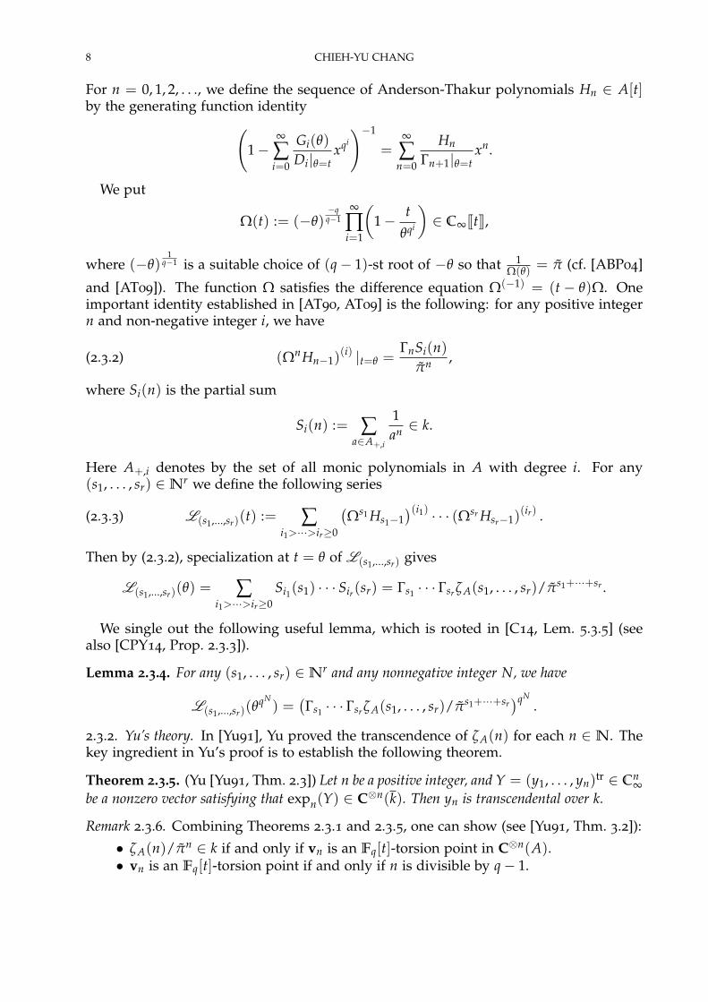
For n = 0, 1, 2, . . ., we define the sequence of Anderson-Thakur polynomials Hn ∈ A[t]by the generating function identity(

1−∞

∑i=0

Gi(θ)

Di|θ=txqi

)−1

=∞

∑n=0

Hn

Γn+1|θ=txn.

We put

Ω(t) := (−θ)−q

q−1∞

∏i=1

(1− t

θqi

)∈ C∞[[t]],

where (−θ)1

q−1 is a suitable choice of (q− 1)-st root of −θ so that 1Ω(θ)

= π (cf. [ABP04]

and [AT09]). The function Ω satisfies the difference equation Ω(−1) = (t − θ)Ω. Oneimportant identity established in [AT90, AT09] is the following: for any positive integern and non-negative integer i, we have

(2.3.2) (ΩnHn−1)(i) |t=θ =

ΓnSi(n)πn ,

where Si(n) is the partial sum

Si(n) := ∑a∈A+,i

1an ∈ k.

Here A+,i denotes by the set of all monic polynomials in A with degree i. For any(s1, . . . , sr) ∈Nr we define the following series

(2.3.3) L(s1,...,sr)(t) := ∑i1>···>ir≥0

(Ωs1 Hs1−1

)(i1) · · · (Ωsr Hsr−1)(ir) .

Then by (2.3.2), specialization at t = θ of L(s1,...,sr) gives

L(s1,...,sr)(θ) = ∑i1>···>ir≥0

Si1(s1) · · · Sir(sr) = Γs1 · · · Γsr ζA(s1, . . . , sr)/πs1+···+sr .

We single out the following useful lemma, which is rooted in [C14, Lem. 5.3.5] (seealso [CPY14, Prop. 2.3.3]).

Lemma 2.3.4. For any (s1, . . . , sr) ∈Nr and any nonnegative integer N, we have

L(s1,...,sr)(θqN) =

(Γs1 · · · Γsr ζA(s1, . . . , sr)/πs1+···+sr

)qN.

2.3.2. Yu’s theory. In [Yu91], Yu proved the transcendence of ζA(n) for each n ∈ N. Thekey ingredient in Yu’s proof is to establish the following theorem.

Theorem 2.3.5. (Yu [Yu91, Thm. 2.3]) Let n be a positive integer, and Y = (y1, . . . , yn)tr ∈ Cn∞

be a nonzero vector satisfying that expn(Y) ∈ C⊗n(k). Then yn is transcendental over k.

Remark 2.3.6. Combining Theorems 2.3.1 and 2.3.5, one can show (see [Yu91, Thm. 3.2]):

• ζA(n)/πn ∈ k if and only if vn is an Fq[t]-torsion point in C⊗n(A).• vn is an Fq[t]-torsion point if and only if n is divisible by q− 1.


2.4. Review of the CPY criterion for Eulerian MZV’s. In what follows, by a Frobeniusmodule we mean a left k[t, σ]-module that is free of finite rank over k[t], where k[t, σ] :=k[t][σ] is the twisted polynomial ring generated by σ over k[t] subject to the relationσ f = f (−1)σ for f ∈ k[t]. Morphisms of Frobenius modules are defined to be left k[t, σ]-module homomorphisms and we denote by F the category of Frobenius modules.

In what follows, an object M in F is said to be defined by a matrix Φ ∈ Matr(k[t]) ifM is free of rank r over k[t] and the σ-action on a given k[t]-basis of M is represented bythe matrix Φ. We denote by 1 the trivial object in F , where the underlying space of 1is k[t] and on which σ acts as σ f = f (−1) for f ∈ 1. We further denote by C⊗n the nthtensor power of the Carlitz motive for n ∈ N. The underlying space of C⊗n is k[t], andon which σ acts by σ f := (t− θ)n f (−1) for f ∈ C⊗n.

By an Anderson t-motive we mean an object M′ ∈ F that possesses the followingproperties.

• M′ is also a free left k[σ]-module of finite rank.• σM′ ⊆ (t− θ)nM′ for all sufficiently large integers n.

Here we follow the terminology of Anderson t-motives in [P08] (cf. [A86, ABP04]).For a fixed Anderson t-motive M′ of rank d over k[σ], we are interested in Ext1

F (1, M′),the set of equivalence classes of Frobenius modules M fitting into a short exact sequenceof Frobenius modules

0→ M′ → M 1→ 0,

and we denote by [M] the equivalence class of M in Ext1F (1, M′). Since Fq[t] is con-

tained inside the center of k[t, σ], left multiplication by any element of Fq[t] on M′ isa morphism and hence Ext1

F (1, M′) has a natural Fq[t]-module structure coming fromBaer sum and pushout of morphisms of M′. The following is a review of the Fq[t]-module isomorphisms established by Anderson

Ext1F (1, M′) ∼= M′/(σ− 1)M′ ∼= E′(k),

where

(2.4.1) E′ = (Gda , ρ)

is the t-module over k associated to M′ in the sense that the k-valued points of E′ isisomorphic to M′/(σ − 1)M′ as Fq-vector spaces and the Fq[t]-module structure on E′

via ρ is induced by the Fq[t]-action on M′/(σ− 1)M′. For a detailed description of theisomorphisms above, see [CPY14, § 5.2]. We also refer the reader to [S97, PR03, HP04,Ta10, BP, CP12, HJ16] for related discussions.

For example, let n be a positive integer. Then the nth tensor power of Carlitz motiveC⊗n has a k[σ]-basis

(t− θ)n−1, . . . , (t− θ), 1

and every f ∈ C⊗n/(σ − 1)C⊗n has a

unique representative polynomial (with degree ≤ n− 1) of the form u1(t− θ)n−1 + · · ·+un ∈ k[t]. Then the maps above can be characterized as

(2.4.2) Ext1F (1, C⊗n) ∼= C⊗n/(σ− 1)C⊗n ∼= C⊗n(k)[

M f]

7→ f 7→ (u1, . . . , un)tr,

where M f ∈ F is defined by the matrix

10 CHIEH-YU CHANG

(2.4.3) Φ f :=(

(t− θ)n 0f (−1)(t− θ)n 1

)∈ Mat2(k[t]).

Remark 2.4.4. For n ∈ N, we note that H(−1)n−1 (t− θ)n = Hn−1 + (σ− 1)Hn−1 in C⊗n and

soH(−1)

n−1 (t− θ)n ≡ Hn−1 ∈ C⊗n/(σ− 1)C⊗n.

The special point vn given in Theorem 2.3.1 is defined to be the image of H(−1)n−1 (t− θ)n

under the isomorphism C⊗n/(σ− 1)C⊗n ∼= C⊗n(k). For the details, see [CPY14, p. 26].

Let Z be an MZV of weight w. Following [T04], we say that Z is Eulerian if the ratioZ/πw is in k. In [CPY14], an effective criterion for Eulerian MZV’s is established and wedescribe it as follows. Let r be a positive integer and fix an r-tuple s = (s1, . . . , sr) ∈ Nr.We define the matrix Φs ∈ Matr+1(k[t]),

(2.4.5) Φs :=

(t− θ)s1+···+sr 0 0 · · · 0H(−1)

s1−1(t− θ)s1+···+sr (t− θ)s2+···+sr 0 · · · 0

0 H(−1)s2−1(t− θ)s2+···+sr . . . ...

... . . . (t− θ)sr 00 · · · 0 H(−1)

sr−1 (t− θ)sr 1

.

Define Φ′s ∈ Matr(k[t]) to be the square matrix of size r cut off from the upper left squareof Φs:

(2.4.6) Φ′s :=

(t− θ)s1+···+sr

H(−1)s1−1(t− θ)s1+···+sr (t− θ)s2+···+sr

. . . . . .

H(−1)sr−1−1(t− θ)sr−1+sr (t− θ)sr

.

Define(2.4.7)

Ψs :=

Ωs1+···+sr

Ωs2+···+srLs1 Ωs2+···+sr

Ωs3+···+srL(s1,s2) Ωs3+···+srLs2. . .

...... . . . Ωsr−1+sr

ΩsrL(s1,...,sr−1)ΩsrL(s2,...,sr−1)

ΩsrLsr−1 Ωsr

L(s1,...,sr) L(s2,...,sr) · · · L(sr−1,sr) Lsr 1

∈ GLr+1(T)

and let

(2.4.8) Ψ′s :=

Ωs1+···+sr

Ωs2+···+srLs1 Ωs2+···+sr

Ωs3+···+srL(s1,s2) Ωs3+···+srLs2. . .

...... . . . Ωsr−1+sr

ΩsrL(s1,...,sr−1)ΩsrL(s2,...,sr−1)

ΩsrLsr−1 Ωsr

∈ GLr(T)


be the square matrix cut off from the upper left square of Ψs. Then we have that

(2.4.9) Ψ′(−1)s = Φ′sΨ

′s and Ψ(−1)

s = ΦsΨs

(see [AT09, C14, CPY14]).We let Ms (resp. M′s) be the Frobenius module defined by the matrix Φs (resp. Φ′s).

Then Ms represents a class in Ext1F (1, M′s) ∼= M′s/(σ − 1)M′s ∼= E′s(k) and we define

vs ∈ E′s(k) to be the image of [Ms] under the composition of the isomorphisms above.Note that it is shown in [CPY14, Thm. 5.3.4] that actually E′s is defined over A and vs isan integral point in E′s(A).

The criterion of Chang-Papanikolas-Yu for Eulerian MZV’s is as follows.

Theorem 2.4.10. [CPY14, Thms. 5.3.5 and 6.1.1] For each r-tuple s = (s1, . . . , sr) ∈ Nr, letE′s and vs be defined as above. Then we explicitly construct a polynomial as ∈ Fq[t] so thatζA(s) is Eulerian if and only if vs is an as-torsion point in E′s(A).

3. Step I: A necessary condition

3.1. The formulation. In this section, our main goal is to show the following necessarycondition, which will be applied to compute the dimension of double zeta values.

Theorem 3.1.1. Let n ≥ 2 be an integer and for i = 1, . . . , m, let si = (si1, si2) ∈N2 be chosenwith si1 + si2 = n. Suppose that we have

(3.1.2) c0ζA(n) +m

∑i=1

ciζA(si) = 0 for some c0, c1, . . . , cm ∈ k.

If the coefficient cj is nonzero for some 1 ≤ j ≤ m, then we have that (q− 1)|sj2. In other words,all k-linear relations among ζA(n), ζA(s1), . . . , ζA(sm) are those coming from the k-linearrelations among ζA(n) ∪

ζA(sj); (q− 1)|sj2

.

Proof. Note that each double zeta value ζA(si) is associated to the system of Frobeniusdifference equations

(3.1.3) Ψ(−1)i = ΦiΨi,

where

Φi :=

(t− θ)n 0 0H(−1)

si1−1(t− θ)n (t− θ)si2 0

0 H(−1)si2−1(t− θ)si2 1

and

Ψi :=

Ωn 0 0Ωsi2L

[i]21 Ωsi2 0

L[i]

31 L[i]

32 1

.

Here for each 1 ≤ i ≤ m,

L[i]

21 := Lsi1 =∞

∑`=0

(Ωsi1 Hsi1−1

)(`) ∈ T

andL

[i]31 := L(si1,si2)

:= ∑`1>`2≥0

(Ωsi2 Hsi2−1

)(`2)(Ωsi1 Hsi1−1

)(`1) ∈ T,

12 CHIEH-YU CHANG

which satisfy for any integer N ∈ Z≥0,(3.1.4)

L[i]

21 (θqN) = (ζA(si1)/πn)qN

and L[i]

31 (θqN) = (ζA(si1, si2)/πn)qN

(see Lemma 2.3.4).

Moreover, ζA(n) is associated to the system of Frobenius difference equations

(3.1.5)(

Ωn

Ln

)(−1)

=

((t− θ)n 0

H(−1)n−1 (t− θ)n 1

)(Ωn

Ln

),

where

Ln :=∞

∑i=0

(ΩnHn−1)(i) ∈ T

has the property that for N ∈ Z≥0,

Ln(θqN) = (ΓnζA(n)/πn)qN

(see Lemma 2.3.4).

To prove this theorem, without loss of generality we assume that each coefficient ci 6= 0for i = 1, . . . , m. Multiplying the equation (3.1.2) by a suitable element in Fq[θ], withoutloss of generality we may assume that ai := ci

Γsi1 Γsi2|θ=t and a0 := c0

Γn|θ=t are in Fq[t] for

i = 1, . . . , m. Note that a1 6= 0, . . . , am 6= 0. So we have that

a0(θ)ΓnζA(n) +m

∑i=1

ai(θ)Γsi1Γsi2ζ(si) = 0.

Define

Φ :=

(t− θ)n

H(−1)s11−1(t− θ)n (t− θ)s12

... . . .

H(−1)sm1−1(t− θ)n (t− θ)sm2

a0H(−1)n−1 (t− θ)n a1H(−1)

s12−1(t− θ)s12 · · · amH(−1)sm2−1(t− θ)sm2 1

∈ Matm+2(k[t])

and

ψ :=

Ωn

Ωs12L[1]

21...

Ωsm2L[m]

21a0Ln + ∑m

i=1 aiL[i]

31

∈ Mat(m+2)×1(T).

Using (3.1.3) and (3.1.5) one has ψ(−1) = Φψ.By hypothesis we have(

a0Ln +m

∑i=1

aiL[i]

31

)(θ) =

c0ζA(n) + ∑mi=1 ciζA(si)

πn = 0.

It follows from the ABP-criterion [ABP04, Thm. 3.1.1] that there exists f = ( f0, f1, . . . , fm, fm+1) ∈Mat1×(m+2)(k[t]) so that

fψ = 0 and f(θ) = (0, . . . , 0, 1).


Put f := 1fm+1

f and note that fψ = 0. We take the (−1)-fold Frobenius twist of the

equation fψ = 0 and then subtract it from itself, and then we have that

(f− f(−1)Φ)ψ = 0.

Note that the last coordinate of the vector f− f(−1)Φ is zero. Define

(R0, R1, . . . , Rm, 0) := f− f(−1)Φ

and note that

(3.1.6)

R0 := f0 − f0(−1)

(t− θ)n −∑mi=1 fi

(−1)H(−1)si1−1(t− θ)n − a0H(−1)

n−1 (t− θ)n

R1 := f1 − f1(−1)

(t− θ)s12 − a1H(−1)s12 (t− θ)s12

...

Rm := ˜fm − ˜fm(−1)

(t− θ)sm2 − amH(−1)sm2−1(t− θ)sm2 ,

where ( f1, · · · , ˜fm, 0) := f. We claim that R0 = R1 = · · · = Rm = 0.Assume this claim first. Put

γ :=

1

1. . .

1f0 f1 . . . ˜fm 1

and note that the claim above implies the following difference equations

γ(−1)Φ =

(Φ′

1

)γ,

where Φ′ is the square matrix of size m + 1 cut off from the upper left square of Φ.By [CPY14, Prop. 2.2.1] the rational functions f0, . . . , ˜fm have a (nonzero) common

denominator b ∈ Fq[t] so that b fi ∈ k[t] for i = 0, 1, . . . , m. Since b(−1) = b, multiplicationby b on the both sides of (3.1.6) shows that if we put

δ :=

1

1. . .

1b f0 b f1 . . . b ˜fm 1

and ν := (ba0H(−1)

n−1 (t− θ)n, ba1H(−1)s12−1(t− θ)s12 , . . . , bamH(−1)

sm2−1(t− θ)sm2) ∈ Mat(m+1)×1(k[t]),then we have

(3.1.7) δ(−1)(

Φ′ν 1

)=

(Φ′

1

)δ.

Let M′ (resp. M) be the Frobenius module defined by Φ′ (resp. Φ) and note that[M] ∈ Ext1

F (1, M′). One checks directly that M′ is an Anderson t-motive (cf. the proofs

14 CHIEH-YU CHANG

of [P08, Prop. 6.1.3] and [CY07, Lem. A.1]). So the action of b on M denoted by b ∗M ∈F , is defined by the matrix

b ∗Φ :=(

Φ′ν 1

)(see [CPY14, §§ 2.4]). So the system of difference equations (3.1.7) implies that b ∗ Mrepresents the trivial class in Ext1

F (1, M′). Furthermore, if we let x0, x1, . . . , xm be ak[t]-basis of M′ on which the action of σ is represented by Φ′, then we have the isomor-phism of Fq[t]-modules (see [CPY14, Thm. 5.2.1]):

Ext1F (1, M′) ∼= M′/(σ− 1)M′

[b ∗M] 7→ b ∗M := ba0H(−1)n−1 (t− θ)nx0 + ∑m

i=1 baiH(−1)si2−1(t− θ)si2 xi + (σ− 1)M′.

Note that M′ fits into the short exact sequence of Frobenius modules

0→ C⊗n → M′ ⊕mi=1C⊗si2 → 0,

where the projection map π : M′ ⊕mi=1C⊗si2 is given by π := (∑m

i=0 gixi 7→ (g1, . . . , gm)).However, since the Fq[t]-linear map (σ − 1) : ⊕m

i=1C⊗si2 → ⊕mi=1C⊗si2 is injective, the

snake lemma shows that we have the following short exact sequence of Fq[t]-modules:

0 → C⊗n/(σ− 1)C⊗n → M′/(σ− 1)M′ ⊕mi=1 (C

⊗si2/(σ− 1)C⊗si2) → 0.b ∗M 7→

(baiH

(−1)si2−1(t− θ)si2

)i

For any s ∈N we recall the identification C⊗s/(σ− 1)C⊗s ∼= C⊗s(k), which is an Fq[t]-

module isomorphism and under which H(−1)s−1 (t− θ)s is mapped to the special point vs ∈

C⊗s(A) (by Remark 2.4.4), itself associated to ζA(s). It follows that (baiH(−1)si2−1(t− θ)si2)i

is mapped to ([bai]si2vsi2)i ∈ ⊕mi=1C⊗si2(A). Since b ∗ M represents the trivial class in

Ext1F (1, M′), b ∗M is also trivial in M′/(σ − 1)M′ and hence [bai]vsi2 = 0 ∈ C⊗si2(A)

for each 1 ≤ i ≤ m. That is, each vsi2 is bai-torsion as bai is nonzero. It follows byRemark 2.3.6 that si2 must be divisible by q− 1 for each 1 ≤ i ≤ m.

To finish the proof, it suffices to prove the claim above. Since si1 + si2 = n for each1 ≤ i ≤ m, without loss of generality we may assume that s12 > s22 > · · · > sm2. Fromthe equation (f− f(−1)Φ)ψ = 0 we have that

(3.1.8) R0Ωn + R1Ωs12L[1]

21 + · · ·+ RmΩsm2L[m]

21 = 0.

Dividing the equation above by Ωsm2 one has

(3.1.9) R0Ωsm1 + R1Ωs12−sm2L[1]

21 + · · ·+ RmL[m]

21 = 0.

Note that Ω has simple zero at each t = θqNfor each N ∈ N. Since each Ri is a rational

function having only finitely many poles, we can pick a sufficiently large integer N sothat Ri is regular at t = θqN

for i = 1, . . . , m. Specializing both sides of the equation(3.1.9) at t = θqN

and using the formula (3.1.4) show that

Rm(θqN) (ζA(sm2)/πsm2)qN

= 0.

Since each MZV is non-vanishing by [T09a] and the equality above is valid for N 0,Rm has to be zero as it has only finitely many zeros.


We turn back to the equation (3.1.8) and repeat the arguments above. We then even-tually have Rm = · · · = R2 = 0 and so obtain

R0Ωn + R1Ωs12L[1]

21 = 0.

Again, by dividing Ωs12 , the arguments above show that R1 = 0 and hence R0 = 0.

Corollary 3.1.10. Let n ≥ 2 be an integer and for i = 1, . . . , m, let si = (si1, si2) ∈ N2 bechosen with si1 + si2 = n. Suppose that we have

c0πn +m

∑i=1

ciζA(si) = 0 for some c0, c1, . . . , cm ∈ k.

If the coefficient cj is nonzero for some 1 ≤ j ≤ m, then we have that (q − 1)|sj2. In otherwords, all k-linear relations among πn, ζA(s1), . . . , ζA(sm) are those coming from the k-linearrelations among πn ∪

ζA(sj); (q− 1)|sj2

.

Proof. If n is A-even, then ζA(n)/πn ∈ k by Carlitz [Ca35]. So the result follows fromTheorem 3.1.1. If n is A-odd (ie., n is not divisible by q− 1), then πn /∈ k∞ and hence πn

is k-linearly independent from all MZV’s as each MZV is in k∞. Therefore, we can putc0 = 0 in Theorem 3.1.1 and the desired result follows.

Remark 3.1.11. The result above shows that the set πn∪

ζA(sj); (q− 1) - sj2

is linearlyindependent over k. It verifies the parity conjecture of Thakur [T09b] in this depth twosetting.

Remark 3.1.12. For an even integer n > 2, Gangl, Kaneko and Zagier [GKZ06, Thms. 1

and 2] showed that

O := (2π√−1)n ∪ ζ(3, n− 3), ζ(5, n− 5), . . . , ζ(n− 3, 3)

is a set of generators for the vector space DZn. Our point of view is that the set Ois generated by (2π

√−1)n and weight n double zeta values ζ(odd, odd), but excluding

ζ(n − 1, 1) (ζ is not defined at 1 and so the odd 1 is special). Note that n2 − 1 is the

cardinality of O and hence Conjecture 1.1.1 in the case of even n > 2 is equivalent to thatthere are dimC Sn(SL2(Z)) independent Q-linear relations among the set O .

When the given weight n ≥ 2 is A-even, we consider the set

OA := πn ∪ ζA(s1, s2)|s1 + s2 = n and (q− 1) - s2 ,

which is the analogue of the set O since each ζA(s1, s2) ∈ OA has the property that s1and s2 are both A-odd. So it is not analogous to Conjecture 1.1.1 as OA is k-linearlyindependent by Corollary 3.1.10.

4. Step II: Logarithmic Interpretation

4.1. The formulation. In this section, our goal is to establish the following result.

Theorem 4.1.1. Let r ≥ 2 be an integer and let s := (s1, . . . , sr) ∈ Nr with n := ∑ri=1 si. Put

s′ := (s2, . . . , sr) and suppose that ζA(s′) is Eulerian, ie., ζA(s2, . . . , sr)/πs2+···+sr ∈ k. Let

16 CHIEH-YU CHANG

αs := as′ ∈ Fq[t] be given in Theorem 2.4.10. Then we explicitly construct an integral pointΞs ∈ C⊗n(A) so that there exists a vector Ys ∈ Cn

∞ of the form

Ys =

∗...

αs(θ)Γs1 · · · Γsr ζA(s1, . . . , sr)

satisfying

expn(Ys) = Ξs.

We divide the proof into the following steps.

4.2. Difference equations arising from algebraic points of C⊗n. For each positive inte-ger n, we denote by logn the logarithm of C⊗n. We first recall the convergence domainDn of logn (see [AT90, Prop. 2.4.3]):

Dn :=

z := (z1, . . . , zn)tr ∈ C⊗n(C∞); |zi|∞ < |θ|

i−n+ nqq−1

∞ for i = 1, . . . , n.

For a fixed nonzero point u = (u1, . . . , un)tr ∈ C⊗n(k) ∩Dn, we define the followingpolynomial associated to u:

(4.2.1) f := fu := u1(t− θ)n−1 + · · ·+ un−1(t− θ) + un ∈ k[t].

We let M f be the Frobenius module defined by the matrix Φ f in (2.4.3) and note that[M f ] ∈ Ext1

F (1, C⊗n).Now we define the series

(4.2.2) L f := f +∞

∑i=1

f (i)

(t− θq)n . . . (t− θqi)n∈ k[[t]],

and note that this kind of series was introduced by Papanikolas [P08] and later on stud-ied in [CY07, C14, M14, CPY14].

Proposition 4.2.3. Let notation and assumptions be as above. Then there exists Ψ f ∈ GL2(T)

so that Ψ(−1)f = Φ f Ψ f . So M f is a t-motive in the sense of [P08].

Proof. Note that by the definition of L f we have

L(−1)f = f (−1) +

∞

∑i=0

f (i)

(t− θ)n · · · (t− θqi)n

= f (−1) +L f

(t− θ)n ,

and hence

(4.2.4)(ΩnL f

)(−1)= f (−1)(t− θ)nΩn + ΩnL f .

It follows that if we put

(4.2.5) Ψ f :=(

Ωn 0ΩnL f 1

),

then we haveΨ(−1)

f = Φ f Ψ f .


The hypotheses of u imply that ΩnL f satisfies the condition of [C14, Lemma 5.3.1],whence ΩnL f is an entire function and therefore M f is a t-motive ( cf. [P08, Prop. 6.1.3]and [CY07, §§ 3.2]).

4.3. Some Lemmas.

Lemma 4.3.1. Let u be a nonzero point in C⊗n(k) ∩Dn, and let y be the last coordinate oflogn(u). Let f ∈ k[t] be the polynomial associated to u given in (4.2.1) and Ψ f be defined in(4.2.5). Then we have

Ψ f (θ) =

(1/πn 0y/πn 1

).

To prove Lemma 4.3.1, we need the following formula due to Papanikolas.

Proposition 4.3.2. (Papanikolas [P14]) We write logn = ∑∞i=0 Piτ

i, where P0 = In and Pi ∈Matn(k). For each positive integer i, the bottom row vector of Pi is given by(

(−1)n−1(θqi − θ)n−1

Lni

, . . . ,(−1)n−`(θqi−` − θ)n−`

Lni

, . . . ,1

Lni

).

Proof of Lemma 4.3.1. As we know that Ωn(θ) = 1/πn, by (4.2.5) it suffices to show that

L f (θ) = y.

We interpret L f as

L f =(

u1(t− θ)n−1 + · · ·+ un−1(t− θ) + un

)+

∞

∑i=1

(t− θqi)n−1uqi

1 + · · ·+ (t− θqi)uqi

n−1 + uqi

n

(t− θq)n . . . (t− θqi)n

.

By specializing at t = θ we have

L f (θ) = un +∞

∑i=1

(−1)n−1(θqi − θ)n−1uqi

1 + · · ·+ (−1)(θqi − θ)uqi

n−1 + uqi

n

Lni

.

Hence by Proposition 4.3.2 we obtain that y = L f (θ).

Lemma 4.3.3. Let n be a positive integer and let Ξ ∈ C⊗n(k) be an algebraic point. Then thereexists a positive integer m and an algebraic point u ∈ C⊗n(k) (depending on m) satisfying

• [tm]n(u) = Ξ (ie., u is a tm-division point of Ξ),• logn(u) converges.

Proof. We recall that expn is an entire function on Cn∞ and is of the form expn = In +

∑∞i=1 Qiτ

i. By the inverse function theorem, there exists open subsets U, V ⊂ Cn∞ so that

expn : U → V is one to one and its inverse is also continuous. Note that as formal powerseries logn is inverse to expn and so logn is defined on V. Since expn is surjective, thereexists a vector X ∈ Cn

∞ for which expn (X) = Ξ.For each positive integer m, ∂[tm]n is an upper triangular matrix with θm down to the

diagonals, and the other nonzero entries off the diagonals have degrees in θ strictly lessthan m. It follows that if we define ‖ ∂[tm]−1

n ‖ to be the maximum of the absolute valuesof entries of ∂[tm]−1

n , then we have

‖ ∂[tm]−1n ‖< |θ|−m

∞ .

18 CHIEH-YU CHANG

Hence, we can pick a sufficiently large integer m for which

∂[tm]−1n (X) ∈ U.

Put u := expn(∂[tm]−1

n (X))∈ V, at which logn converges. By the functional equation of

expn, we observe that

[tm]n (u) = [tm]n(

expn

(∂[tm]−1

n (X)))

= expn (X) = Ξ.

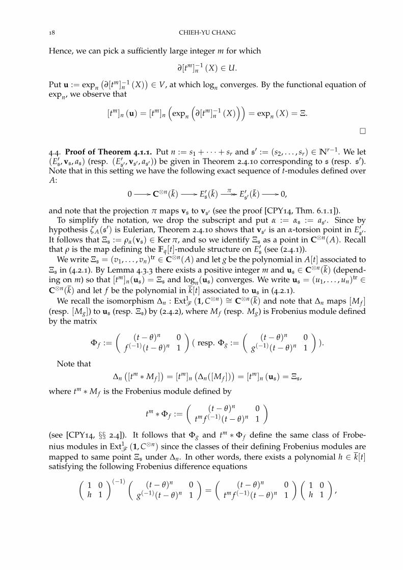
4.4. Proof of Theorem 4.1.1. Put n := s1 + · · ·+ sr and s′ := (s2, . . . , sr) ∈ Nr−1. We let(E′s, vs, as) (resp. (E′s′ , vs′ , as′)) be given in Theorem 2.4.10 corresponding to s (resp. s′).Note that in this setting we have the following exact sequence of t-modules defined overA:

0 // C⊗n(k) // E′s(k)π // // E′s′(k) // 0,

and note that the projection π maps vs to vs′ (see the proof [CPY14, Thm. 6.1.1]).To simplify the notation, we drop the subscript and put α := αs := as′ . Since by

hypothesis ζA(s′) is Eulerian, Theorem 2.4.10 shows that vs′ is an α-torsion point in E′s′ .

It follows that Ξs := ρα(vs) ∈ Ker π, and so we identify Ξs as a point in C⊗n(A). Recallthat ρ is the map defining the Fq[t]-module structure on E′s (see (2.4.1)).

We write Ξs = (v1, . . . , vn)tr ∈ C⊗n(A) and let g be the polynomial in A[t] associated toΞs in (4.2.1). By Lemma 4.3.3 there exists a positive integer m and us ∈ C⊗n(k) (depend-ing on m) so that [tm]n(us) = Ξs and logn(us) converges. We write us = (u1, . . . , un)tr ∈C⊗n(k) and let f be the polynomial in k[t] associated to us in (4.2.1).

We recall the isomorphism ∆n : Ext1F (1, C⊗n) ∼= C⊗n(k) and note that ∆n maps [M f ]

(resp. [Mg]) to us (resp. Ξs) by (2.4.2), where M f (resp. Mg) is Frobenius module definedby the matrix

Φ f :=(

(t− θ)n 0f (−1)(t− θ)n 1

)( resp. Φg :=

((t− θ)n 0

g(−1)(t− θ)n 1

)).

Note that

∆n([tm ∗M f ]

)= [tm]n

(∆n([M f ])

)= [tm]n (us) = Ξs,

where tm ∗M f is the Frobenius module defined by

tm ∗Φ f :=(

(t− θ)n 0tm f (−1)(t− θ)n 1

)(see [CPY14, §§ 2.4]). It follows that Φg and tm ∗ Φ f define the same class of Frobe-nius modules in Ext1

F (1, C⊗n) since the classes of their defining Frobenius modules aremapped to same point Ξs under ∆n. In other words, there exists a polynomial h ∈ k[t]satisfying the following Frobenius difference equations(

1 0h 1

)(−1) ( (t− θ)n 0g(−1)(t− θ)n 1

)=

((t− θ)n 0

tm f (−1)(t− θ)n 1

)(1 0h 1

),


from which we derive the following identity

(4.4.1)

(Ir

h(−1), 0, . . . , 0 1

)(Φ′

g(−1)(t− θ)n, 0, . . . , 0 1

)=

(Φ′

tm f (−1)(t− θ)n, 0, . . . , 0 1

)(Ir

h, 0, . . . , 0 1

),

where Φ′ := Φ′s is given in (2.4.6).We define the following two matrices

Φg :=(

Φ′

g(−1)(t− θ)n, 0, . . . , 0 1

)and Φtm f :=

(Φ′

tm f (−1)(t− θ)n, 0, . . . , 0 1

).

Let Ψ′ := Ψ′s ∈ GLr(T) (resp. Ψ := Ψs ∈ GLr+1(T)) be given in (2.4.8) (resp. (2.4.7)) andnote that Ψ is of the form

Ψ =

(Ψ′µ 1

),

whereµ =

(L(s1,...,sr), . . . , Lsr

).

We further put

Ψtm f :=(

Ψ′tmΩnL f , 0, . . . , 0 1

)and note that using (2.4.9) we have

Ψ(−1)tm f = Φtm f Ψtm f .

Claim: There exists a matrix ν of the form

ν =

(Ir

ν1, . . . , νr 1

)∈ GLr+1(k[t])

so thatν(−1) (α ∗Φ) = Φtm f · ν,

where

Φ := Φs :=(

Φ′ϕ 1

)given in (2.4.5),

and

α ∗Φ :=(

Φ′αϕ 1

).

We first assume the claim above to finish the proof. Define

α ∗Ψ :=(

Ψ′αµ 1

)∈ GLm+1(T).

Since α ∈ Fq[t], using (2.4.9) we have

(α ∗Ψ)(−1) = α ∗Φ · α ∗Ψ.

Note that the claim above implies

(ν · α ∗Ψ)(−1) = ν(−1) · α ∗Φ · α ∗Ψ = Φtm f (ν · α ∗Ψ) .

20 CHIEH-YU CHANG

In other words, ν · α ∗Ψ is also a fundamental matrix for Φtm f in the sense of [P08, §§ 4.1.6]and hence by [P08, § 4.1.6] that there exists a matrix γ ∈ GLr+1(Fq(t)) of the form

γ =

(Ir

γ1, . . . , γr 1

)so that

ν · α ∗Ψ = Ψtm f · γ.

By comparing with the (r + 1, 1)-entries of both sides of the equation above we obtainthe following identity

(4.4.2) ν1Ωn + ν2Ωs2+···+srLs1 + · · ·+ νrΩsrL(s1,...,sr−1)+ αL(s1,...,sr) = tmΩnL f + γ1.

By Lemma 2.3.4 we have that for each N ∈ Z≥0

L(s1,...,sr)(θqN) = L(s1,...,sr)(θ)

qN= (Γs1 · · · Γsr ζA(s1, . . . , sr)/πn)qN

,

and by Lemma 4.3.1 and [CPY14, Prop. 2.3.3] we have that for each N ∈ Z≥0,(ΩnL f

)(θqN

) =(ΩnL f

)(θ)qN

= (y/πn)qN,

where y is the last coordinate of logn(us) as f is the polynomial associated to us. Wemention that γ1 must be in Fq[t] since all other terms of (4.4.2) are in the Tate algebra T.Note that Ω has a simple zero at t = θqN

for each N ∈N and hence by Lemma 2.3.4

Ωs2+···+srL(s1)(θqN

) = · · · = ΩsrL(s1,...,sr−1)(θqN

) = 0.

It follows that specializing (4.4.2) at t = θqNfor a positive integer N and taking the qN-th

root we obtain the following identity

α(θ)Γs1 · · · Γsr ζA(s) = θmy + γ1(θ)πn.

Now we putYs := ∂[tm]n · logn(us) + ∂[γ1]nλn

and note that the last coordinate of Ys is θmy + γ1(θ)πn = α(θ)Γs1 · · · Γsr ζA(s). Since

∂[γ1]nλn ∈ Λn, by the functional equation of expn we see that expn(Ys) = [tm]n (us) = Ξs,whence completing the proof of Theorem 4.1.1.

The rest task is to prove the claim above. We recall that M′ is the Frobenius moduledefined by the matrix Φ′ with respect to a k[t]-basis m1, . . . , mr of M′, and we have thefollowing isomorphism as Fq[t]-modules

Ext1F

(1, M′

) ∼= E′s(k)

and note that [M] is mapped to vs. Hence [α ∗M] is mapped to

Ξs := ρα(vs) ∈ C⊗n(A) → E′s(A).

We note that M′ is a free left k[σ]-module with a natural k[σ]-basis:

(4.4.3)(t− θ)s1+···+sr−1m1, · · · , (t− θ)m1, m1, . . . , (t− θ)sr−1mr, . . . , (t− θ)mr, mr

(see [CPY14, Proof of Thm. 5.2.1]). We recall that g ∈ A[t] is the polynomial associatedto Ξs and hence via the isomorphism Ext1

F (1, M′) ∼= E′s(k), the class of the Frobenius


module defined by the matrix Φg is mapped to Ξs ∈ C⊗n(A) → E′s(A) via the basis(4.4.3) (see [CPY14, (5.2.2)]). In other words, the two matrices Φg and

α ∗Φ =

(Φ′ 0

0, . . . , αH(−1)sr−1 (t− θ)sr 1

)define the same class of Frobenius modules in Ext1

F (1, M′). Therefore there exists amatrix

δ =

(Ir

δ1, . . . , δr 1

)∈ GLr+1(k[t])

so that

(4.4.4) δ(−1) · α ∗Φ = Φg · δ.

Put

η :=(

Ir 0h, 0, . . . , 0 1

)∈ GLr+1(k[t])

and note that by (4.4.1) we have η(−1) · Φg = Φtm f · η. Putting ν := ηδ ∈ GLr+1(k[t]) andusing (4.4.4) and (4.4.1) we have the desired identity

ν(−1) · α ∗Φ = η(−1)δ(−1) · α ∗Φ = η(−1) · Φg · δ = Φtm f · ηδ = Φtm f · ν.

From the explicit forms of δ and η we see that ν has the desired form, whence provingthe claim above.

5. Step III: The Identity

5.1. The dimension formula. In this section, we will give a proof of Theorem 1.2.1 (1).Combining Theorems 4.1.1 and 2.3.5, we first prove the following.

Theorem 5.1.1. Let n ≥ 2 be an integer and let vn ∈ C⊗n(A) be the special point given inTheorem 2.3.1. For s = (s1, . . . , sr) ∈Nr with r ≥ 2, we denote by s′ := (s2, . . . , sr). Put

En :=s = (s1, . . . , sr) ∈Nr; r ≥ 2, wt(s) = n and ζA(s

′) is Eulerian

.

For each s ∈ En, let Ξs ∈ C⊗n(A) be given in Theorem 4.1.1. Then we have

dimk Spank πn, ζA(n), ζA(s); s ∈ En = 1 + rankFq[t]SpanFq[t] vn ∪s∈En Ξs .

Proof. To prove the theorem, it suffices to prove the following equivalent statements:

πn, ζA(n), ζA(s); s ∈ En are linearly dependent over k

⇔ vn ∪s∈En Ξs are linearly dependent over Fq[t].

Proof of (⇒). Suppose that there exist polynomials (not all zero) η∪ηss∈En⊆ Fq[t]

for which[η]n(vn) + ∑

s∈En

[ηs]n (Ξs) = 0.

By Theorem 2.3.1, there exists a vector Yn of the form

Yn =

∗...

ΓnζA(n)

∈ Cn∞

22 CHIEH-YU CHANG

for which expn(Yn) = vn. For each s ∈ En, by Theorem 4.1.1 there exists vectors Ys ∈ Cn∞

satisfying the property in Theorem 4.1.1. We define the vector

Y := ∂[η]nYn + ∑s∈En

∂[ηs]nYs

and note that

expn(Y) = [η]n (expn(Yn)) + ∑s∈En

[ηs]n (expn(Ys)) = [η]n(vn) + ∑s∈En

[ηs]n (Ξs) = 0,

whenceY ∈ Ker expn = ∂[Fq[t]]nλn.

Note that the last coordinate of λn is πn and that for each a ∈ Fq[t], ∂[a]n is an uppertriangular matrix with a(θ) down the diagonals. Taking the last coordinates from bothsides of the equality above gives the desired result.

Proof of (⇐). We suppose that there exist polynomials δ0, δ, δs; s ∈ En ∈ A (not allzero) so that

δ0πn + δζA(n) + ∑s∈En

δsζA(s) = 0,

which can be also written as

δ0πn +δ

ΓnΓnζA(n) + ∑

s∈En

δsαs(θ)Γs

αs(θ)ΓsζA(s) = 0,

where Γs := Γs1 . . . Γsr for s = (s1, . . . , sr) and αs ∈ Fq[t] is given in Theorem 4.1.1.Multiplying a common denominator of the coefficients of the equation above shows thatthere exist polynomials η0, η, ζs; s ∈ En ⊆ Fq[t] (not all zero) so that

η0(θ)πn + η(θ)ΓnζA(n) + ∑

s∈En

ηs(θ)αsΓsζA(s) = 0.

For each s ∈ En, let Ys ∈ Cn∞ be given in Theorem 4.1.1 and note that its last coordinate

is αs(θ)ΓsζA(s). So the last coordinate of

Y := ∂[η0]nλn + ∂[η]nYn + ∑s∈En

∂[ηs]nYs

is zero by the equation above. Since

expn(Y) = expn

(∂[η0]nλn + ∂[η]nYn + ∑

s∈En

∂[ηs]nYs

)= [η]n (vn)+ ∑

s∈En

[ηs]n (Ξs) ∈ C⊗n(A),

Theorem 2.3.5 implies that Y has to be zero, and hence

[η]n (vn) + ∑s∈En

[ηs]n (Ξs) = 0.

Remark 5.1.2. For a positive integer n, we recall that ζA(n)/πn ∈ k for A-even n by [Ca35]and in which case vn is an Fq[t]-torsion point by Remark 2.3.6. When n is A-odd, wehave πn /∈ k∞ and so πn is k-linearly independent from MZV’s, whence from the proofabove we derive that

[η]n(vn) + ∑s∈En

[ηs]n(Ξs) = 0


if and only if

η(θ)ΓnζA(n) + ∑s∈En

ηs(θ)ΓsζA(s) = 0

for η ∪s∈En ηs ⊆ Fq[t].

By this remark, we immediately obtain the following two consequences.

Corollary 5.1.3. For an integer n ≥ 2, we continue with the notation in Theorem 5.1.1. Thenwe have

dimk Spank ζA(n), ζA(s); s ∈ En

=

1 + rankFq[t]SpanFq[t] Ξs; s ∈ En if n is A-even,

rankFq[t]SpanFq[t] vn, Ξs; s ∈ En if n is A-odd.

Corollary 5.1.4. Let n ≥ 2 be a positive integer. Put

V :=(s1, s2) ∈N2; s1 + s2 = n and (q− 1)|s2

.

For each s ∈ V , let Ξs be given in Theorem 4.1.1. Then we have

dimk Spank πn, ζA(s); s ∈ V = 1 + rankFq[t]SpanFq[t] Ξss∈V .

5.2. Proof of Theorem 1.2.1 (1). Here we give a proof for part (1) of Theorem 1.2.1,which is addressed as the following result.

Corollary 5.2.1. Let n ≥ 2 be an integer. Put

S := πn, ζA(1, n− 1), ζA(2, n− 2), . . . , ζA(n− 1, 1) ,

and

V :=(s1, s2) ∈N2; s1 + s2 = n and (q− 1)|s2

.

For each s ∈ V , let Ξs be given in Theorem 4.1.1. Then we have

dimk SpankS = n− bn− 1q− 1

c+ rankFq[t] SpanFq[t] Ξss∈V .

Proof. Note that we have the following equalities

dimk SpankS = |S \ πn, ζA(s); s ∈ V |+ dimk Spank πn, ζA(s); s ∈ V =

(n− 1− bn−1

q−1 c)+(

1 + rankFq[t] SpanFq[t] Ξss∈V

)= n− bn−1

q−1 c+ rankFq[t] SpanFq[t] Ξss∈V ,

where the first equality comes from Corollary 3.1.10, and the second equality comesfrom Corollary 5.1.4.

Remark 5.2.2. Recently, some algebraic independence results of certain MZV’s are ob-tained by Mishiba [M14], but the coordinates of those MZV’s are restricted to be A-oddwith other hypotheses. Concerning this issue, we refer the reader to [M14].

24 CHIEH-YU CHANG

6. Step IV: A Siegel’s Lemma

6.1. The main result. The primary result in this section is the following theorem, whichimplies Theorem 1.2.1 (2) and so allows us to compute the exact quantity in Theo-rem 1.2.1 (1).

Theorem 6.1.1. Let n be a positive integer and v1, . . . , vm ∈ C⊗n(A). Then we have an effectivealgorithm to compute the following rank

rm := rankFq[t]SpanFq[t] v1, . . . , vm .

Proof. We let vi := (vi1, . . . , vin)tr ∈ C⊗n(A), and let fi := vi1(t− θ)n−1 + · · ·+ vin ∈ A[t]

be its associated polynomial. Note that the class [Mi] ∈ Ext1F (1, C⊗n) ∼= C⊗n(k) is

mapped to vi, where Mi ∈ F is defined by the matrix((t− θ)n 0

f (−1)i (t− θ)n 1

).

Fix m polynomials a1, . . . , am ∈ Fq[t] and put F := ∑mi=1 ai fi. Then the class [MF] ∈

Ext1F (1, C⊗n) is mapped to the integral point ∑m

i=1[ai]nvi (see [CPY14, §§ 2.4]), whereMF ∈ F is defined by the matrix(

(t− θ)n 0F(−1)(t− θ)n 1

).

It follows that ∑mi=1[ai]nvi = 0 if and only if MF presents the trivial class in Ext1

F (1, C⊗n).Therefore, we have the following equivalence:

• ∑mi=1[ai]nvi = 0 ∈ C⊗n(A).

• there exists a polynomial δ ∈ k[t] for which(1 0δ 1

)(−1) ( (t− θ)n 0F(−1)(t− θ)n 1

)=

((t− θ)n 0

0 1

)(1 0δ 1

),

which is equivalent to

(6.1.2) δ(−1)(t− θ)n + F(−1)(t− θ)n = δ.

Step I. Assume that there exist a1, . . . , am ∈ Fq[t] for which ∑mi=1[ai]nvi = 0, ie., the

equation (6.1.2) holds. Then the δ in (6.1.2) must be in A[t].Proof of Step I. Note that the equation (6.1.2) is equivalent to δ(t− θq)n + F(t− θq)n =

δ(1). Then the result follows from H.-J. Chen’s formulation in the proof of [KL15,Thm. 2 (a)].

For a polynomial h = ∑i uiti ∈ A[t], we define its sup-norm by ‖ h ‖:= maxi |ui|∞.Note that for h1, h2 ∈ A[t] we have:

• ‖ h1h2 ‖=‖ h1 ‖ · ‖ h2 ‖.• ‖ h1 + h2 ‖≤ max ‖ h1 ‖, ‖ h2 ‖.

For each vi, we define ‖ vi ‖:= max1≤j≤n|vij|∞

, and note that

‖ fi ‖≤‖ vi ‖ ·|θ|n−1∞ .

PutD := max1≤i≤m ‖ vi ‖ · |θ|n−1

∞


and so‖ F ‖≤ D.

Step II. Let hypotheses be given as in Step I. Define

` := max

log|θ|∞ D + 1,nq

q− 1+ 1

.

Then degθ δ < ` when we regard δ as a polynomial in the variable θ over Fq[t].Proof of Step II. Suppose on the contrary that degθ δ ≥ `, ie., ‖ δ ‖≥ |θ|`∞. Note that

by the definition of ` we have

(6.1.3) ‖ F(t− θq)n ‖< |θ|`∞ · |θ|qn∞ ≤‖ δ(t− θq)n ‖ .

Therefore, (6.1.3) and the equality

δ(t− θq)n + F(t− θq)n = δ(1)

imply that‖ δ(t− θq)n ‖=‖ δ(1) ‖ .

In other words, we have that

degθ δ + nq = q degθ δ,

whencedegθ δ =

nqq− 1

< `,

a contradiction.Step III: End of proof. Now we write

(6.1.4) δ := c1θ`−1 + · · ·+ c` ∈ Fq[t][θ] and F = d1θ`−1 + · · ·+ d` ∈ Fq[t][θ]

and note that the coefficients d1, . . . , d` are Fq[t]-linear combinations of a1, . . . , am. Werecall that solving a1, . . . , am in the equation

m

∑i=1

[ai]n(vi) = 0

is equivalent to solving for δ and a1, . . . , am satisfying

δ(t− θq)n + F(t− θq)n = δ(1).

However, putting the forms of δ and F (6.1.4) into the equation above and compar-ing the coefficients of each θi for i = 0, . . . , ` − 1 we obtain a system of linear equa-tions in c1, . . . , c`, a1, . . . , am over Fq[t]. Using Gauss elimination we can solve for so-lutions c1, . . . , c`, a1, . . . , am effectively, and particularly obtain the rank of the solutionsa1, . . . , am, whence establishing the desired result.

Remark 6.1.5. We mention that in [De91, De92] Denis studied the question of Siegel’slemma type for t-modules. For integral points v1, . . . , vm ∈ C⊗n(A), Denis showedthat there exists a constant c (depending on n and v1, . . . , vm) so that the degrees of thecoefficients of any Fq[t]-linear relations among v1, . . . , vm can be bounded by c. However,the value of c is not explicit in Denis’ results, and our approach is entirely different fromhis.

26 CHIEH-YU CHANG

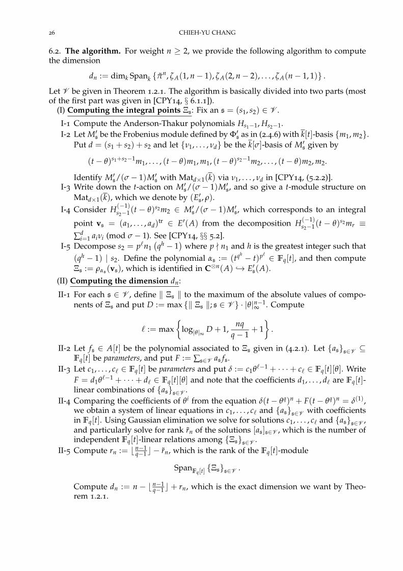
6.2. The algorithm. For weight n ≥ 2, we provide the following algorithm to computethe dimension

dn := dimk Spank πn, ζA(1, n− 1), ζA(2, n− 2), . . . , ζA(n− 1, 1) .

Let V be given in Theorem 1.2.1. The algorithm is basically divided into two parts (mostof the first part was given in [CPY14, § 6.1.1]).

(I) Computing the integral points Ξs: Fix an s = (s1, s2) ∈ V .

I-1 Compute the Anderson-Thakur polynomials Hs1−1, Hs2−1.I-2 Let M′s be the Frobenius module defined by Φ′s as in (2.4.6) with k[t]-basis m1, m2.

Put d = (s1 + s2) + s2 and let ν1, . . . , νd be the k[σ]-basis of M′s given by

(t− θ)s1+s2−1m1, . . . , (t− θ)m1, m1, (t− θ)s2−1m2, . . . , (t− θ)m2, m2.

Identify M′s/(σ− 1)M′s with Matd×1(k) via ν1, . . . , νd in [CPY14, (5.2.2)].I-3 Write down the t-action on M′s/(σ− 1)M′s, and so give a t-module structure on

Matd×1(k), which we denote by (E′s, ρ).I-4 Consider H(−1)

s2−1(t − θ)s2m2 ∈ M′s/(σ − 1)M′s, which corresponds to an integral

point vs = (a1, . . . , ad)tr ∈ E′(A) from the decomposition H(−1)

s2−1(t − θ)s2mr ≡∑d

i=1 aiνi (mod σ− 1). See [CPY14, §§ 5.2].I-5 Decompose s2 = p`n1

(qh − 1

)where p - n1 and h is the greatest integer such that

(qh − 1) | s2. Define the polynomial αs := (tqh − t)p` ∈ Fq[t], and then computeΞs := ραs(vs), which is identified in C⊗n(A) → E′s(A).

(II) Computing the dimension dn:

II-1 For each s ∈ V , define ‖ Ξs ‖ to the maximum of the absolute values of compo-nents of Ξs and put D := max ‖ Ξs ‖; s ∈ V · |θ|n−1

∞ . Compute

` := max

log|θ|∞ D + 1,nq

q− 1+ 1

.

II-2 Let fs ∈ A[t] be the polynomial associated to Ξs given in (4.2.1). Let ass∈V ⊆Fq[t] be parameters, and put F := ∑s∈V as fs.

II-3 Let c1, . . . , c` ∈ Fq[t] be parameters and put δ := c1θ`−1 + · · ·+ c` ∈ Fq[t][θ]. WriteF = d1θ`−1 + · · ·+ d` ∈ Fq[t][θ] and note that the coefficients d1, . . . , d` are Fq[t]-linear combinations of ass∈V .

II-4 Comparing the coefficients of θi from the equation δ(t− θq)n + F(t− θq)n = δ(1),we obtain a system of linear equations in c1, . . . , c` and ass∈V with coefficientsin Fq[t]. Using Gaussian elimination we solve for solutions c1, . . . , c` and ass∈V ,and particularly solve for rank rn of the solutions [as]s∈V , which is the number ofindependent Fq[t]-linear relations among Ξss∈V .

II-5 Compute rn := bn−1q−1 c − rn, which is the rank of the Fq[t]-module

SpanFq[t] Ξss∈V .

Compute dn := n− bn−1q−1 c+ rn, which is the exact dimension we want by Theo-

rem 1.2.1.


6.3. Computational data. In this section, we list some data of implementing the algo-rithm above using Magma. We thank Yi-Hsuan Lin for providing the code. In whatfollows, “Weight‘’ means the weight n, and “Dimension” means dn above, and “Fp-linear” means the number of independent linear relations arising from (1.2.2). When theweight n is A-odd (ie., (q− 1) - n) the author does not know whether (1.2.2) can producea linear relation as ζA(r)ζA(s) is a “monomial” for one at least of r, s being A-odd. Sowe let the position of A-odd weight be blank. “Zeta-like” means the number of weightn double zeta values ζA(s) for which ζA(s)/ζA(n) ∈ k. We list the computation databelow only for q = 2 and q = 3, although we have run the program for other q up to 11with weight up to 150.

For q = 2, we have:

Weight 2 3 4 5 6 7 8 9 10 11 12 13 14 15

Dimension 1 2 2 3 3 3 3 4 4 4 4 5 5 5

Fp-linear 0 1 1 1 2 2 2 3 3 3 4 4 4 5

Zeta-like 1 1 1 0 0 2 1 0 0 0 0 0 0 2

16 17 18 19 20 21 22 23 24 25 26 27 28 29 30

5 6 6 6 6 7 7 7 7 8 8 8 8 8 8

5 5 6 6 6 7 7 7 8 8 8 9 9 9 10

0 0 0 0 0 0 0 0 0 0 0 0 0 0 0

31 32 33 34 35 36 37 38 39 40 41 42 43 44 45

8 8 9 9 9 9 10 10 10 10 11 11 11 11 11

10 10 11 11 11 12 12 12 13 13 13 14 14 14 15

2 0 0 0 0 0 0 0 0 0 0 0 0 0 0

46 47 48 49 50 51 52 53 54 55 56 57 58 59 60

11 11 11 12 12 12 12 12 12 12 12 13 13 13 13

15 15 16 16 16 17 17 17 18 18 18 19 19 19 20

0 0 0 0 0 0 0 0 0 0 0 0 0 0 0

61 62 63 64 65 66 67 68 69 70 71 72 73 74 75

13 13 13 13 14 14 14 14 15 15 15 15 16 16 16

20 20 21 21 21 22 22 22 23 23 23 24 24 24 25

0 0 2 0 0 0 0 0 0 0 0 0 0 0 0

76 77 78 79 80 81 82 83 84 85 86 87 88 89 90

16 16 16 16 16 17 17 17 17 17 17 17 17 18 18

25 25 26 26 26 27 27 27 28 28 28 29 29 29 30

0 0 0 0 0 0 0 0 0 0 0 0 0 0 0

91 92 93 94 95 96 97 98 99 100 101 102 103 104 105

18 18 18 18 18 18 19 19 19 19 19 19 19 19 20

30 30 31 31 31 32 32 32 33 33 33 34 34 34 35

0 0 0 0 0 0 0 0 0 0 0 0 0 0 0

106 107 108 109 110 111 112 113 114 115 116 117 118 119 120

20 20 20 20 20 20 20 21 21 21 21 21 21 21 21

35 35 36 36 36 37 37 37 38 38 38 39 39 39 40

0 0 0 0 0 0 0 0 0 0 0 0 0 0 0

28 CHIEH-YU CHANG

For q = 3, we have:

Weight 3 4 5 6 7 8 9 10 11 12 13 14 15 16

Dimension 3 4 5 5 7 7 8 9 10 10 12 12 13 13

Fp-linear 0 0 1 1 1 1 2

Zeta-like 1 0 1 1 1 1 1 0 0 0 0 0 0 0

17 18 19 20 21 22 23 24 25 26 27 28 29 30 31

14 14 16 16 17 17 18 18 19 19 20 21 22 22 24

2 2 2 3 3 3 3

2 0 0 0 0 0 2 0 3 2 2 0 0 0 0

32 33 34 35 36 37 38 39 40 41 42 43 44 45 46

24 25 25 26 26 28 28 29 29 30 30 31 31 32 33

4 4 4 4 5 5 5 5

0 0 0 0 0 0 0 0 0 0 0 0 0 0 0

47 48 49 50 51 52 53 54 55 56 57 58 59 60 61

34 34 35 35 36 36 37 37 39 39 40 40 41 41 42

6 6 6 6 7 7 7

0 0 0 0 0 0 2 0 0 0 0 0 0 0 0

62 63 64 65 66 67 68 69 70 71 72 73 74 75 76

42 43 44 45 45 46 46 47 47 48 48 50 50 51 51

7 8 8 8 8 9 9 9

0 0 0 0 0 0 0 0 0 2 0 0 0 0 0

77 78 79 80 81 82 83 84 85 86 87 88 89 90 91

52 52 53 53 54 55 56 56 58 58 59 59 60 60 62

9 10 10 10 10 11 11

4 0 3 2 0 0 0 0 0 0 0 0 0 0 0

92 93 94 95 96 97 98 99 100 101 102 103 104 105 106

62 63 63 64 64 65 65 66 67 68 68 69 69 70 70

11 11 12 12 12 12 13 13

0 0 0 0 0 0 0 0 0 0 0 0 0 0 0

107 108 109 110 111 112 113 114 115 116 117 118 119 120 121

71 71 73 73 74 74 75 75 76 76 77 78 79 79 80

13 13 14 14 14 14 15

0 0 0 0 0 0 0 0 0 0 0 0 0 0 0

122 123 124 125 126 127 128 129 130 131 132 133 134 135 136

80 81 81 82 82 84 84 85 85 86 86 87 87 88 89

15 15 15 16 16 16 16 17

0 0 0 0 0 0 0 0 0 0 0 0 0 0 0

137 138 139 140 141 142 143 144 145 146 147 148 149 150

90 90 91 91 92 92 93 93 95 95 96 96 97 97

17 17 17 18 18 18 18

0 0 0 0 0 0 0 0 0 0 0 0 0 0


References

[A86] G. W. Anderson, t-motives, Duke Math. J. 53 (1986), no. 2, 457–502.[ABP04] G. W. Anderson, W. D. Brownawell and M. A. Papanikolas, Determination of the algebraic relations

among special Γ-values in positive characteristic, Ann. of Math. (2) 160 (2004), no. 1, 237–313.[AT90] G. W. Anderson and D. S. Thakur, Tensor powers of the Carlitz module and zeta values, Ann. of Math.

(2) 132 (1990), no. 1, 159–191.[AT09] G. W. Anderson and D. S. Thakur, Multizeta values for Fq[t], their period interpretation, and relations

between them, Int. Math. Res. Not. IMRN (2009), no. 11, 2038–2055.[Andre04] Y. Andre, Une introduction aux motifs (motifs purs, motifs mixtes, periodes), Panoramas et

Syntheses, 17. Societe Mathematique de France, Paris, 2004.[B12] F. Brown, Mixed Tate motives over Z, Ann. of Math. (2) 175 (2012), no. 2, 949–976.[BP] W. D. Brownawell and M. A. Papanikolas, A rapid introduction to Drinfeld modules, t-modules, and

t-motives, available at http://www.math.tamu.edu/∼map/BanffSurvey.pdf, 2011.[Ca35] L. Carlitz, On certain functions connected with polynomials in a Galois field, Duke Math. J. 1 (1935),

no. 2, 137-168.[Cart02] P. Cartier, Fonctions polylogarithmes, nombres polyzetas et groupes pro-unipotents, Seminaire Bourbaki,

Vol. 2000/2001. Asterisque No. 282 (2002), Exp. No. 885, viii, 137-173.[C14] C.-Y. Chang, Linear independence of monomials of multizeta values in positive characteristic, Compos.

Math. 150 (2014), no. 11, 1789-1808.[CP12] C.-Y. Chang and M. A. Papanikolas, Algebraic independence of periods and logarithms of Drinfeld

modules. With an appendix by Brian Conrad. J. Amer. Math. Soc. 25 (2012), no. 1, 123–150.[CPY14] C.-Y. Chang, M. A. Papanikolas and J. Yu, An effective criterion for Eulerian multizeta values in

positive characteristic, arXiv:1411.0124.[CY07] C.-Y. Chang and J. Yu, Determination of algebraic relations among special zeta values in positive char-

acteristic, Adv. Math. 216 (2007), no. 1, 321-345.[Chen15] H.-J. Chen, On shuffle of double zeta values for Fq[t], J. Number Theory, 148 (2015), 153-163.[Chen16] H.-J. Chen, On shuffle of double Eisenstein series in positive characteristic, in preparation.[DG05] P. Deligne, A. B. Goncharov, Groupes fondamentaux motiviques de Tate mixte, Ann. Sci. Ecole Norm.

Sup. (4) 38 (2005), no. 1, 1-56.[De91] L. Denis, Geometrie diophantienne sur les modules de Drinfel’d, The arithmetic of function fields

(Columbus, OH, 1991), 285-302, Ohio State Univ. Math. Res. Inst. Publ., 2, de Gruyter, Berlin,1992.

[De92] L. Denis, Hauteurs canoniques et modules de Drinfeld, Math. Ann. 294, 213-223 (1992).[GKZ06] H. Gangl, M. Kazeko and D. Zagier, Double zeta values and modular forms, Automorphic forms

and zeta functions, 71-106, World Sci. Publ., Hackensack, NJ, 2006.[Ge88] E.U. Gekeler, On the coefficients of Drinfeld modular forms, Invent. Math. 93 (1988), no. 3, 667-700.[Gon97] A. B. Goncharov, The double logarithm and Manin’s complex for modular curves, Math. Res. Lett., 4

(1997), 617-636.[Go80] D. Goss, Modular forms for Fr[T], J. Reine Angew. Math. 317 (1980), 16-39.[Go96] D. Goss, Basic structures of function field arithmetic, Springer-Verlag, Berlin, 1996.[HJ16] U. Hartl and A.-K. Juschka, Pink’s theory of Hodge structures over function fields, available at

www.math.uni-muenster.de/u/urs.hartl/Publikat/Hodge2.pdf, 2016.[HP04] U. Hartl and R. Pink, Vector bundles with a Frobenius structure on the punctured unit disc, Compos.

Math. 140 (2004), no. 3, 689–716.[IKZ06] L. Ihara, M. Kaneko and D. Zagier, Derivation and double shuffle relations for multiple zeta values,

Compos. Math.142 (2006), no. 2, 307-338.[KL15] Y.-L. Kuan and Y.-H. Lin, Criterion for deciding zeta-like multizeta values in positive characteristic,

Exp. Math. 25 (2016), no. 3, 246–256.[LRT14] J. A. Lara Rodrıguez and D. S. Thakur, Zeta-like multizeta values for Fq[t], Indian J. Pure Appl.

Math. 45 (5), 785-798 (2014).[M14] Y. Mishiba, On algebraic independence of certain multizeta values in characteristic p, arXiv:1401.3628.[P08] M. A. Papanikolas, Tannakian duality for Anderson-Drinfeld motives and algebraic independence of

Carlitz logarithms, Invent. Math. 171 (2008), no. 1, 123–174.[P14] M. A. Papanikolas, Log-algebraicity on tensor powers of the Carlitz module and special values of Goss

L-function, in preparation.

30 CHIEH-YU CHANG

[PR03] M. A. Papanikolas and N. Ramachandran, A Weil-Barsotti formula for Drinfeld modules, J. NumberTheory 98 (2003), no. 2, 407–431.

[S97] S. K. Sinha, Periods of t-motives and transcendence, Duke Math. J. 88 (1997), no. 3, 465–535.[Ta10] L. Taelman, 1-t-motifs, arXiv:0908.1503, 2010.[Te02] T. Terasoma, Mixed Tate motives and multiple zeta values, Invent. Math. 149 (2002), no. 2, 339-369.[T04] D. S. Thakur, Function field arithmetic, World Scientific Publishing, River Edge NJ, 2004.[T09a] D. S. Thakur, Power sums with applications to multizeta and zeta zero distribution for Fq[t], Finite

Fields Appl. 15 (2009), no. 4, 534-552.[T09b] D. S. Thakur, Relations between multizeta values for Fq[T], Int. Math. Res. Notices IMRN (2009),

no. 12, 2318–2346

[T10] D. S. Thakur, Shuffle relations for function field multizeta values, Int. Math. Res. Not. IMRN (2010),no. 11, 1973-1980.

[To15] G. Todd, Linear relations between multizeta values, Ph.D. Thesis, University of Arizona (2015).[Yu91] J. Yu, Transcendence and special zeta values in characteristic p, Ann. of Math. (2) 134 (1991), no. 1,

1–23.[Z93] D. Zagier, Periods of modular forms, traces of Hecke operators, and multiple zeta values, Research into

automorphic forms and L functions (Japanese) (Kyoto, 1992). Srikaisekikenkysho Kkyroku No.843 (1993), 162170.

[Z94] D. Zagier, Values of zeta functions and their applications, First European Congress of Mathematics,Vol. II (Paris, 1992), Progress in Math. 120, Birkhuser-Verlag, Basel, (1994) 497-512.

[Zh16] J. Zhao, Multiple zeta functions, multiple polylogarithms and their special values, Series on NumberTheory and its Applications, 12. World Scientific Publishing Co. Pte. Ltd., Hackensack, NJ, 2016.

Department of Mathematics, National Tsing Hua University, Hsinchu City 30042, Taiwan R.O.C.E-mail address: [email protected]

linear relations among double zeta values in positive...

Documents