linkage, crossing over, & chromosome mapping in...
TRANSCRIPT

Chapter 7. Linkage, Crossing Over, & Chromosome Mapping in Eukaryotes 1. Linkage, Recombination, and Crossing over 2. Chromosome Mapping 3. Cytogenetic Mapping
1
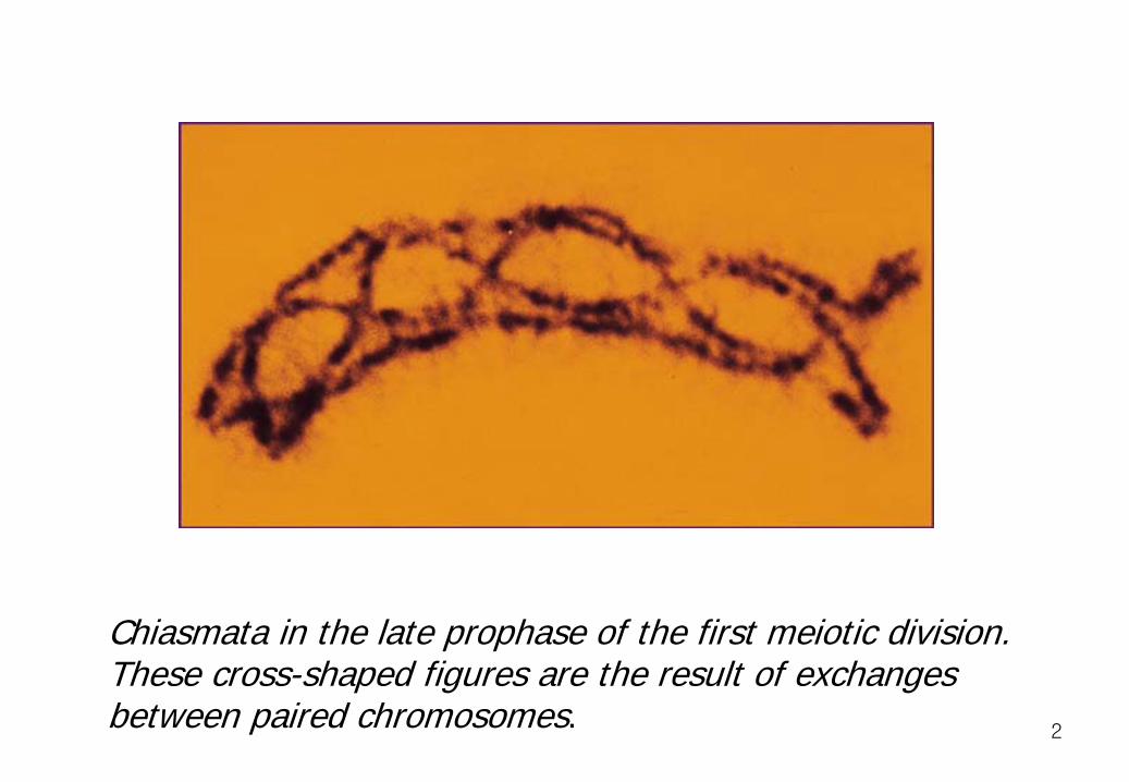
Chiasmata in the late prophase of the first meiotic division. These cross-shaped figures are the result of exchanges between paired chromosomes.
2

The World's First Chromosome Map chromosome organization emerged from a combination of genetic and cytological studies. T. H. Morgan laid the foundation for these studies when he demonstrated that the gene for white eyes in Drosophila was located on the X chromosome. The map was a straight line, and each gene was situated at a particular point, or locus, on it Locus: A fixed position on a chromosome that is occupied by a given gene or one of its alleles.
3

One night in 1911 Sturtevant, undergraduate working in Morgan's laboratory put aside his algebra homework in order to evaluate some experimental data. Before the sun rose the next day, he had constructed the world's first chromosome map.
4

No microscope was powerful enough to see genes, nor was any measuring device accurate enough to obtain the distances between them. In fact, Sturtevant did not use any sophisticated instruments in his work. Instead, he relied completely on the analysis of data from experimental crosses with Drosophila.
5

1. Linkage, Recombination, and Crossing Over Sturtevant based his mapping procedure on the principle that genes on the same chromosome should be inherited together. Because such genes are physically attached to the same structure, they should travel as a unit through meiosis. This phenomenon is called linkage. Linkage: A relationship among genes in the same chromosome. Such genes tend to be inherited together.
6
The early geneticists also knew that linkage was not absolute. Their experimental data demonstrated that genes on the same chromosome could be separated as they went through meiosis and that new combinations of genes could be formed. However, this phenomenon, called recombination, was difficult to explain by simple genetic theory.
7

One hypothesis was that during meiosis, when homologous chromosomes paired, a physical exchange of material separated and recombined genes. cytological observation
A crossover point was called a chiasma (plural, chiasmata), from the Greek word meaning “cross.” 8
Exceptions to the Mendelian principle of independent assortment
Bateson and Punett sweet peas two traits, flower color and pollen length Red flower, long pollen grain are dominant. 9:3:3:1 ???
9
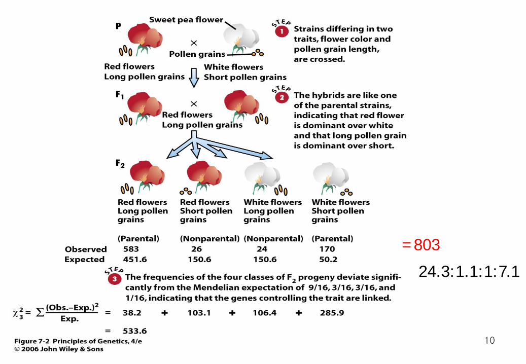
24.3:1.1:1:7.1 =803
10
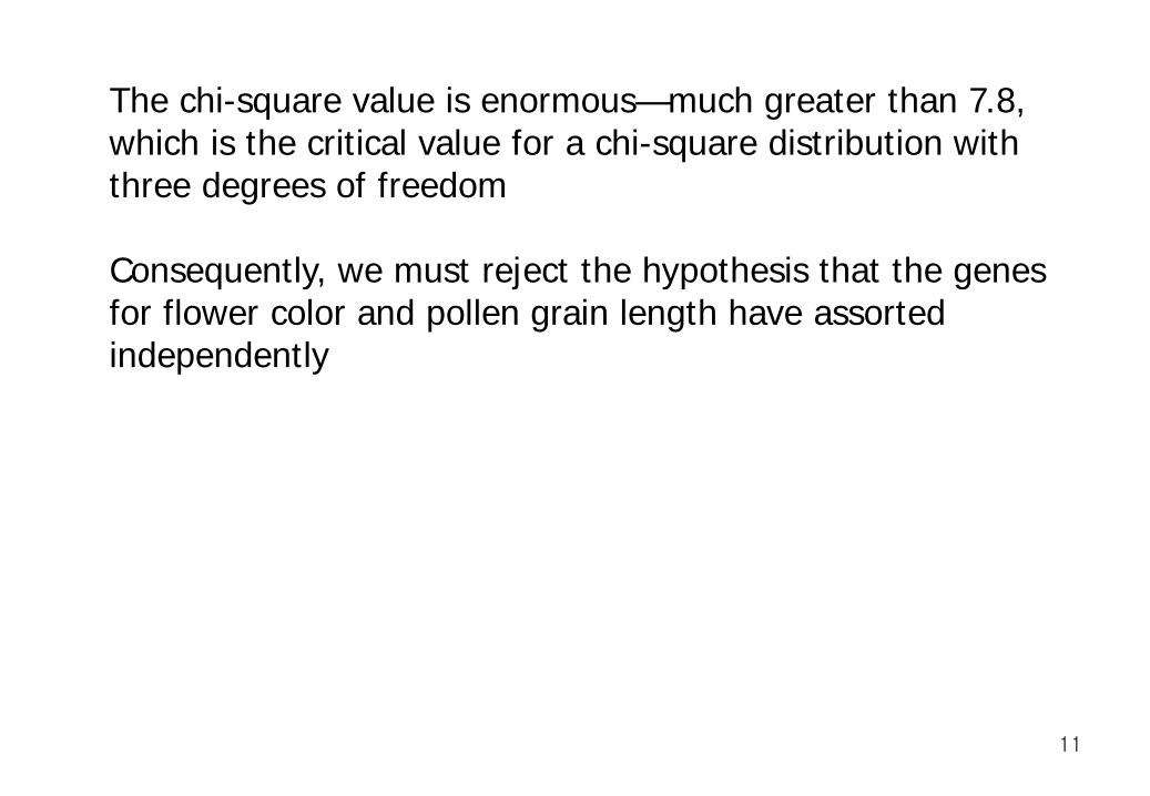
The chi-square value is enormous—much greater than 7.8, which is the critical value for a chi-square distribution with three degrees of freedom Consequently, we must reject the hypothesis that the genes for flower color and pollen grain length have assorted independently
11

Some nonparental progeny do appear, although at low frequency. Because these progeny indicate that the alleles of the two genes were recombined in the F1, they are called recombinants.
12

Frequency of recombination as a measure of linkage intensity
We can use the frequency of recombination to measure the intensity of linkage between genes. Genes that are tightly linked seldom recombine, whereas genes that are loosely linked recombine often.
13

Each phenotype is highlighted by a different color in the Punnett square. These phenotypes do not appear in a 9:3:3:1 ratio because the genes for flower color and pollen length are located on the same chromosome.
14

Frequency of recombination as a measure of linkage intensity
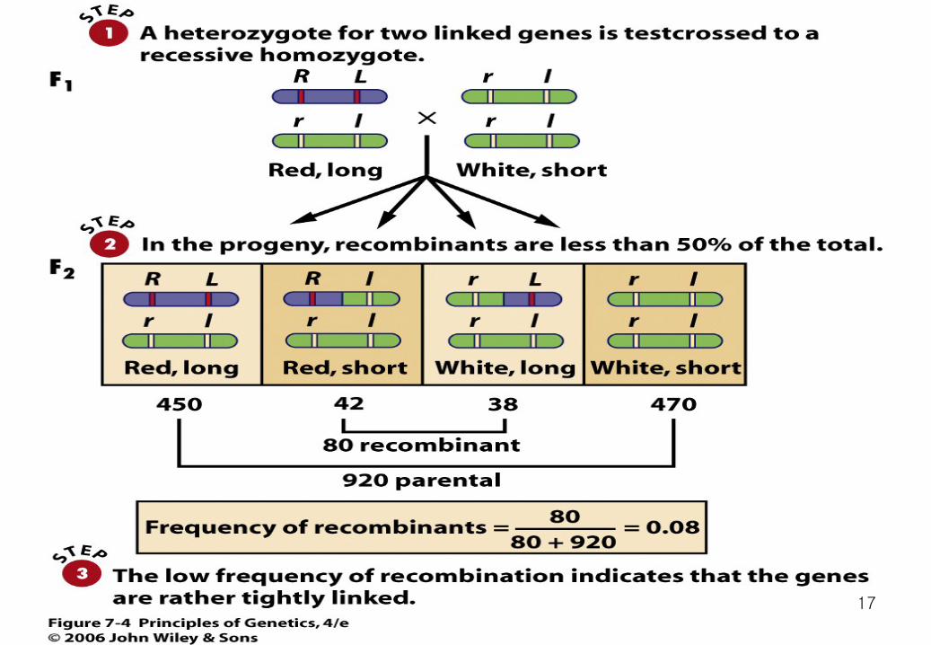
The most direct way of estimating the frequency of recombination is to use a testcross, in which the individual to be analyzed genetically is crossed to a homozygote carrying the recessive alleles.
15

AA BB individual is crossed to an aa bb individual. From this cross, the Aa Bb offspring are then testcrossed to the double recessive parent. Because the A and B genes assort independently, the F2 will consist of two classes (Aa Bb and aa bb) that are phenotypically like the parents in the original cross, and two classes (Aa bb and aa Bb) that are phenotypically recombinant. Furthermore, each F2 class will occur with a frequency of 25 percent.
16
17

For any two genes, the frequency of recombinant gametes never exceeds 50 percent. This upper limit is reached when genes are very far apart, perhaps at opposite ends of a chromosome. It is also reached when genes are on different chromosomes; 50 percent recombination is, in fact, what is meant when it is said that the genes assort independently.
18
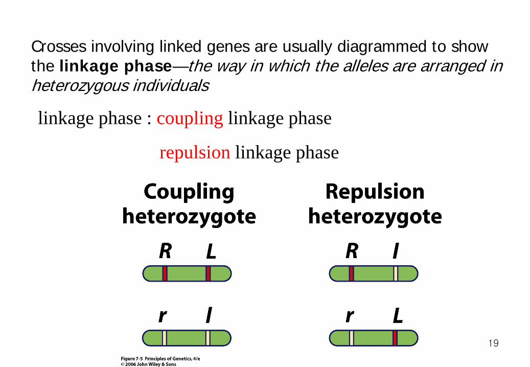
Crosses involving linked genes are usually diagrammed to show the linkage phase—the way in which the alleles are arranged in heterozygous individuals
linkage phase : coupling linkage phase
repulsion linkage phase
19

Crossing Over as the Physical Basis of Recombination Recombinant gametes are produced as a result of crossing over between homologous chromosomes. The exchange event occurs during the prophase of the first meiotic division, when duplicated chromosomes have paired. Although four homologous chromatids are present, forming what is called a tetrad, only two chromatids cross over at any one point.
20
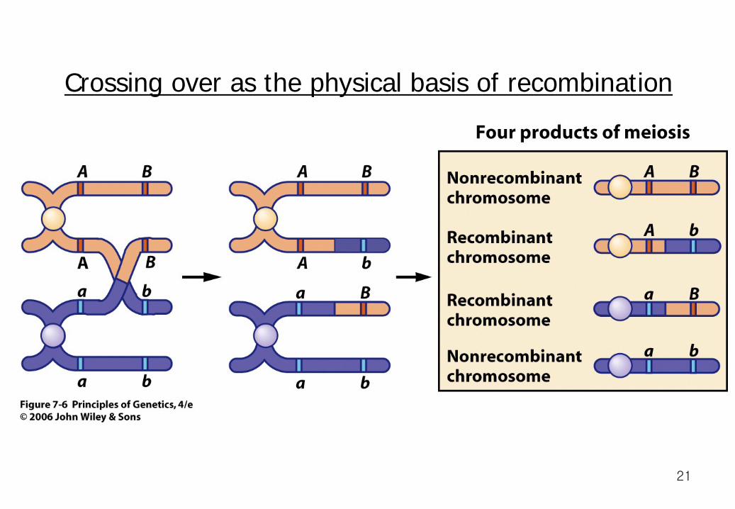
Crossing over as the physical basis of recombination
21
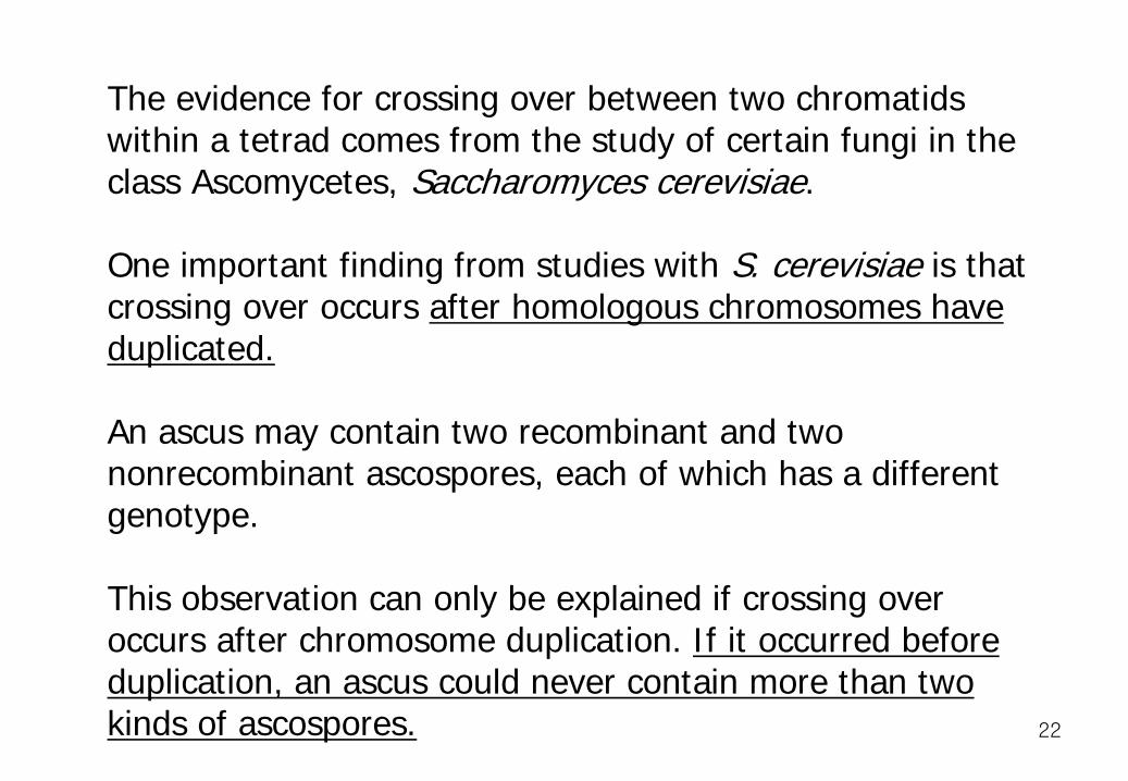
The evidence for crossing over between two chromatids within a tetrad comes from the study of certain fungi in the class Ascomycetes, Saccharomyces cerevisiae. One important finding from studies with S. cerevisiae is that crossing over occurs after homologous chromosomes have duplicated. An ascus may contain two recombinant and two nonrecombinant ascospores, each of which has a different genotype. This observation can only be explained if crossing over occurs after chromosome duplication. If it occurred before duplication, an ascus could never contain more than two kinds of ascospores. 22

A second finding is that only two chromatids are involved in an exchange at any one point. However, the other two chromatids may cross over at a different point. Thus, there is a possibility for multiple exchanges in a tetrad of chromatids
23

24

25

Evidence That Crossing Over Causes Recombination In 1931 Harriet Creighton and Barbara McClintock obtained evidence that genetic recombination was associated with a material exchange between chromosomes. Creighton and McClintock studied homologous chromosomes in maize that were morphologically distinguishable. The goal was to determine whether physical exchange between these homologues was correlated with recombination between some of the genes they carried.
26
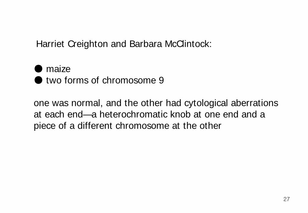
Harriet Creighton and Barbara McClintock: ● maize ● two forms of chromosome 9 one was normal, and the other had cytological aberrations at each end—a heterochromatic knob at one end and a piece of a different chromosome at the other
27

Evidence that crossing over causes recombination
● Kernel color ( C, colored ; c, colorless ) ● Kernel texture (Wx, starchy ; wx, waxy )
28

Evidence that crossing over causes recombination
29

x
Chiasmata and the Time of Crossing Over The cytological evidence for crossing over can be seen during late prophase of the first meiotic division when the chiasmata become clearly visible.
30

Diplonema of male meiosis in the grasshopper Chorthippus parallelus
x
As we might expect, large chromosomes typically have more chiasmata than small chromosomes. Thus, the number of chiasmata is roughly proportional to chromosome length. When the heat shocks were administered late in prophase, there was little effect, but when they were given earlier, the recombination frequency was changed.
31
x
Although almost all the DNA is synthesized during the interphase that precedes the onset of meiosis, a small amount is made during the first meiotic prophase. This limited DNA synthesis has been interpreted as part of a process to repair broken chromatids, which, as we have discussed, is thought to be associated with crossing over.
32

x
33

2. Chromosome Mapping 1) Crossing over as a measure of genetic distance Sturtevant's fundamental insight was to estimate the distance between points on a chromosome by counting the number of crossovers between them. Points that are far apart should have more crossovers between them than points that are close together.
In a statistical sense. The distance between two points on the genetic map of a chromosome is the average number of crossovers between them. 34
35
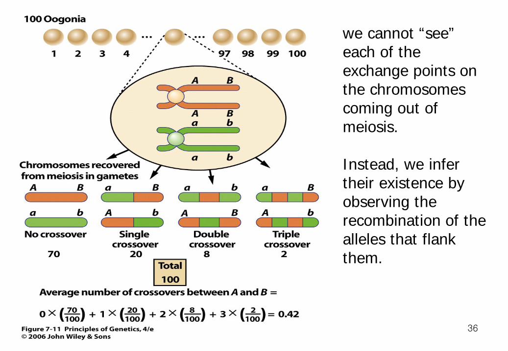
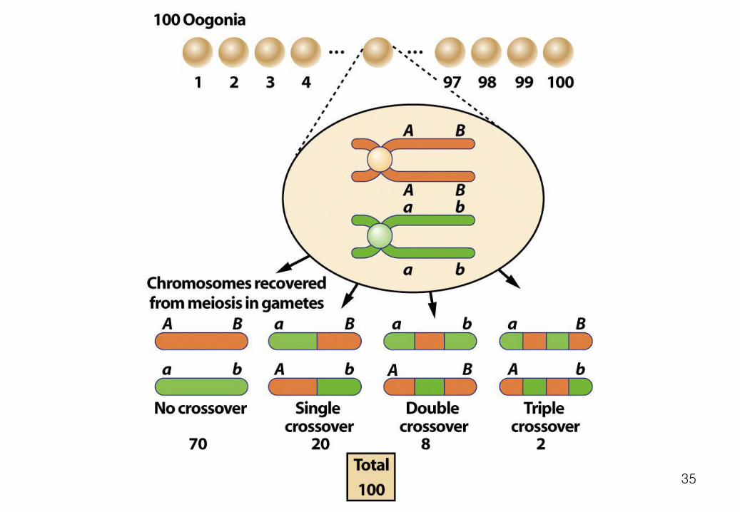
we cannot “see” each of the exchange points on the chromosomes coming out of meiosis. Instead, we infer their existence by observing the recombination of the alleles that flank them.
36
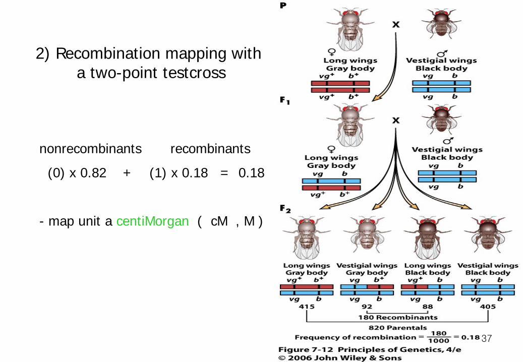
nonrecombinants recombinants (0) x 0.82 + (1) x 0.18 = 0.18 - map unit a centiMorgan ( cM , M )
2) Recombination mapping with a two-point testcross
37

3) Recombination mapping with a three-point testcross Determination of the gene order Three possible gene orders: (i) sc ec cv (ii) ec sc cv (iii) ec cv sc cv ec sc
38

39
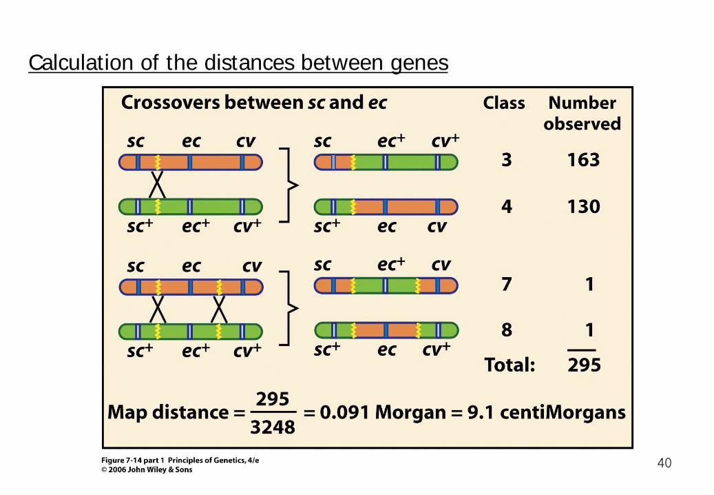
Calculation of the distances between genes
40

Calculation of the distances between genes
41
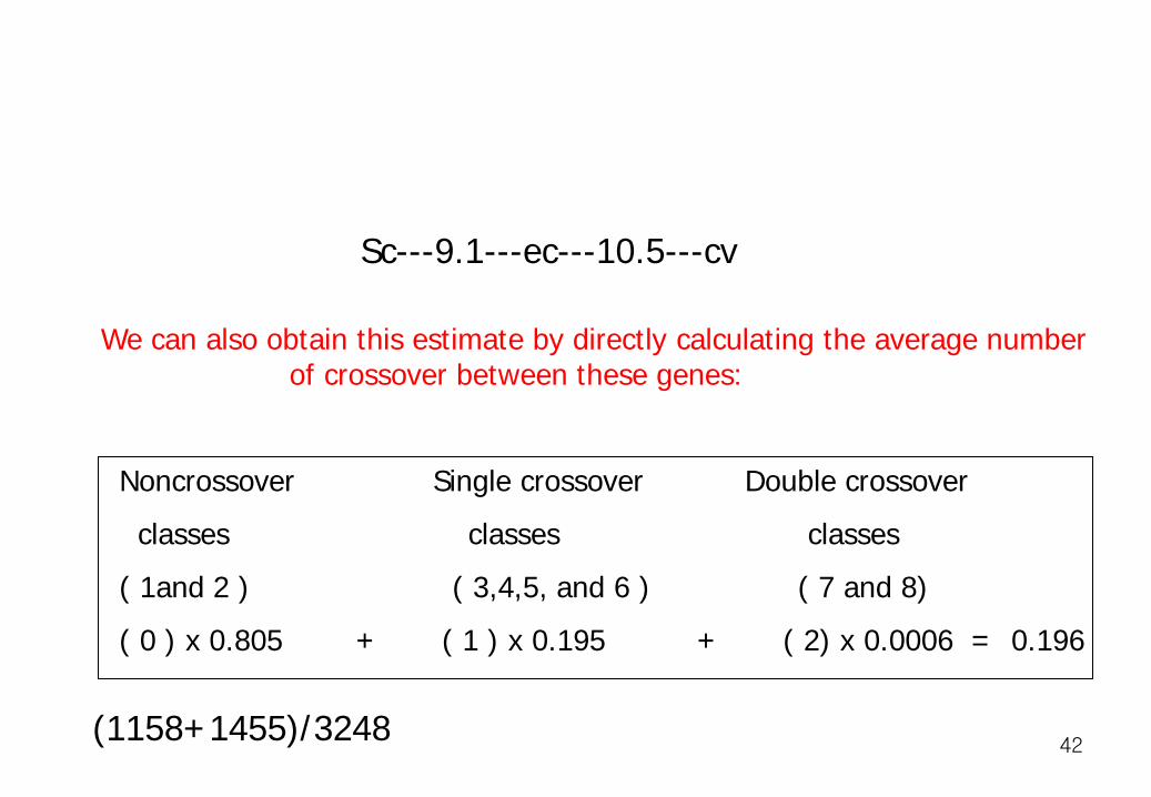
We can also obtain this estimate by directly calculating the average number of crossover between these genes:
Noncrossover Single crossover Double crossover classes classes classes ( 1and 2 ) ( 3,4,5, and 6 ) ( 7 and 8) ( 0 ) x 0.805 + ( 1 ) x 0.195 + ( 2) x 0.0006 = 0.196
Sc---9.1---ec---10.5---cv
(1158+1455)/3248 42

4) Interference and the coefficient of coincidence A three-point cross has an important advantage over a two-point cross: it allows the detection of double crossovers, permitting us to determine if exchanges in adjacent regions are independent of each other. Does a crossover in the region between sc and ec (region I on the map of the X chromosome) occur independently of a crossover in the region between ec and cv (region II)? Or does one crossover inhibit the occurrence of another nearby?
43

one crossover inhibited the occurrence of another nearby, a phenomenon called interference. The extent of the interference is customarily measured by the coefficient of coincidence, c, which is the ratio of the observed frequency of double crossovers to the expected frequency:
44
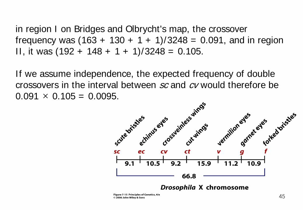
in region I on Bridges and Olbrycht's map, the crossover frequency was (163 + 130 + 1 + 1)/3248 = 0.091, and in region II, it was (192 + 148 + 1 + 1)/3248 = 0.105. If we assume independence, the expected frequency of double crossovers in the interval between sc and cv would therefore be 0.091 × 0.105 = 0.0095.
45
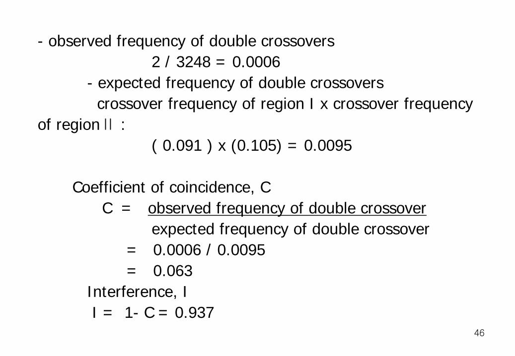
- observed frequency of double crossovers 2 / 3248 = 0.0006 - expected frequency of double crossovers crossover frequency of region I x crossover frequency of regionⅡ : ( 0.091 ) x (0.105) = 0.0095 Coefficient of coincidence, C C = observed frequency of double crossover expected frequency of double crossover = 0.0006 / 0.0095 = 0.063 Interference, I I = 1- C = 0.937
46

5) Recombination frequency and genetic map distance A discrepancy between map distance and percent recombination.
47

As an example, let us consider the genes at the ends of Bridges and Olbrycht's map of the X chromosome; sc, at the left end, was 66.8 cM away from f, at the right end. However, the frequency of recombination between sc and f was 50 percent—the maximum possible value. Using this frequency to estimate map distance, we would conclude that sc and f were 50 map units apart.
48

49

Multiple crossovers may occur between widely separated genes, and some of these crossovers may not produce genetically recombinant chromosomes
50
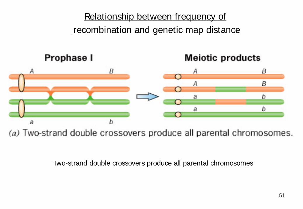
Relationship between frequency of recombination and genetic map distance
Two-strand double crossovers produce all parental chromosomes
51

Relationship between frequency of recombination and genetic map distance
52
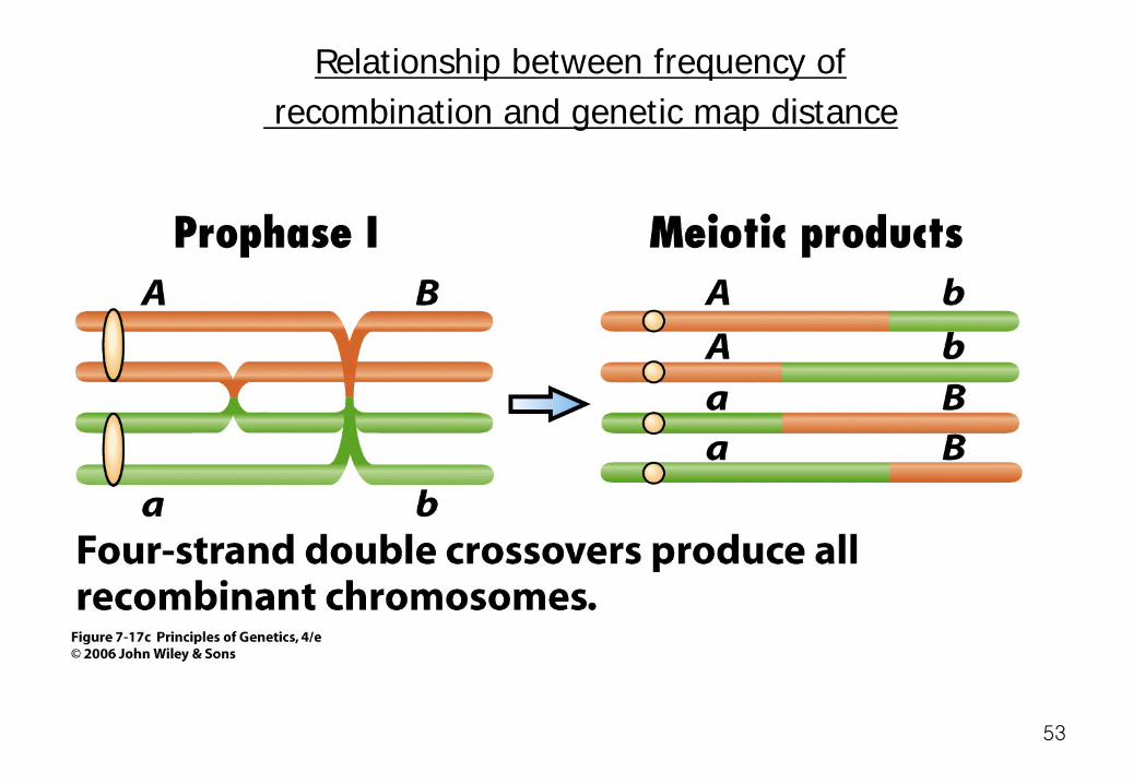
Relationship between frequency of recombination and genetic map distance
53

This second example shows that a double crossover may not contribute to the frequency of recombination, even though it contributes to the average number of exchanges on a chromosome. A quadruple crossover would have the same effect. These and other multiple exchanges are responsible for the discrepancy between recombination frequency and genetic map distance.
54
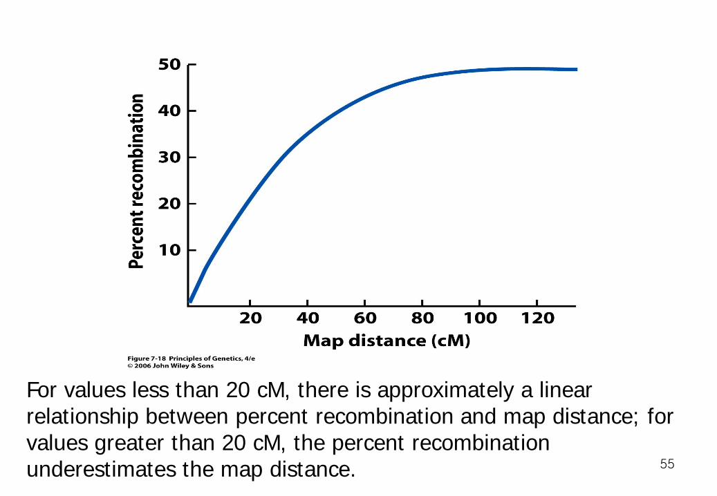
For values less than 20 cM, there is approximately a linear relationship between percent recombination and map distance; for values greater than 20 cM, the percent recombination underestimates the map distance. 55

6) Chiasma frequency and genetic map distance
Each chiasma is thought to represent the resolution of a crossover that occurred earlier in prophase. Thus, by counting chiasmata, we should be able to estimate the average number of crossovers occurring on a chromosome, which we can then use as an estimate of genetic map length. Let's suppose, for example, that in a group of 100 cells going through meiosis, 5 cells show five chiasmata in a particular pair of chromosomes, 15 show four chiasmata in this pair, 15 show three, 30 show two, 25 show one, and 10 show none
56

This translates into an average of 1.07 chiasmata per chromatid because each chiasma affects only two of the four chromatids in the chromosome pair
57

3. Cytogenetic Mapping Recombination mapping allows us to determine the relative positions of genes by using the frequency of crossing over as a measure of distance. However, it does not allow us to localize genes with respect to cytological landmarks, such as bands, on chromosomes. This kind of localization requires a different procedure that involves studying the phenotypic effects of chromosome rearrangements, such as deletions and duplications. The map positions of those genes can be tied to locations on the cytological map of a chromosome. This process, called cytogenetic mapping 58

cytologically defined deletion (or deficiency, usually symbolized Df) 59

60

We can also use duplications to determine the cytological locations of genes. We look for a duplication that masks the phenotype of a recessive mutation.
61

62

The basic principle in deletion mapping is that a deletion that uncovers a recessive mutation must lack a wild-type copy of the mutant gene. This fact localizes that gene within the boundaries of the deletion. The basic principle in duplication mapping is that a duplication that covers a recessive mutation must contain a wild-type copy of the mutant gene. This fact localizes that gene within the boundaries of the duplication.
63
We expect that long chromosomes should have more crossovers than short ones and that this relationship will be reflected in the lengths of their genetic maps. For the most part, our assumption is true; however, within a chromosome some regions are more prone to crossing over than others. Thus, distances on the genetic map do not correspond exactly to physical distances along the chromosome's cytological map
4. Genetic Distance and Physical Distance
64
Crossing over is less likely to occur near the ends of a chromosome and also around the centromere; consequently, these regions are condensed on the genetic map. Other regions, in which crossovers occur more frequently, are expanded.
65

1) Genetic distance and physical distance
66

Even though there is not a uniform relationship between genetic and physical distance, the genetic and cytological maps of a chromosome are colinear; that is, particular sites have the same order. Recombination mapping therefore reveals the true order of the genes along a chromosome. However, it does not tell us the actual physical distances between them.
67

2) Detecting linked loci by pedigree analysis To detect and analyze linkage in humans, geneticists must collect data from pedigrees. Often these data are limited or incomplete, or the information they provide is ambiguous. Challenge Today, modern molecular methods permit researchers to analyze the inheritance of dozens of different markers in the same set of pedigrees.
68
In addition, breakthroughs in cytogenetics and cell culture techniques have allowed geneticists to tie these maps to individual chromosomes and to localize genes to specific regions within them.
The linkage relationships that are easiest to study in human beings are those between genes on the X chromosome. Determining linkage between autosomal genes is much more difficult. The human genome has 22 different autosomes, and a gene that does not show X-linkage could be on any one of them.
69
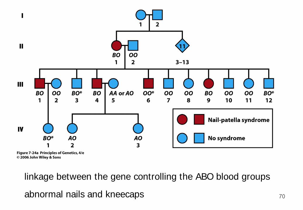
linkage between the gene controlling the ABO blood groups
abnormal nails and kneecaps 70

The woman in generation II must represent a new occurrence of the NPS1 mutation. Neither of her parents nor any of her 11 siblings showed the nail-patella phenotype. Among the five individuals who showed the nail-patella syndrome in this pedigree, all but one (III-6) of them had blood type B. NPS1 is linked to the B allele 71

If we assume this inference to be correct, then the woman in generation II must have the genotype NPS1 B/ + O;. Her husband's genotype is clearly + O/ + O.
72

The mating is a testcross. However, only 3 (III-3, III-6, III-12) of their 10 children were recombinants; the other 7 were nonrecombinants. Thus, we can estimate the frequency of recombination, 3/10 = 30 percent. 73

However, this estimate does not use all the information in the pedigree. the information from the couples' three grandchildren, only one (IV-1) of whom was a recombinant. Altogether, then, 3 + 1 = 4 of the 10 + 3 = 13 offspring in the pedigree were recombinants. Thus, we conclude that the frequency of recombination between the NPS1 and ABO loci is 4/13 = 31 percent. 31cM (later, more data 10cM) 74

The first localization of a gene to a specific human autosome came in 1968, when R. P. Donahue and coworkers demonstrated that the Duffy blood group locus, denoted FY, is on chromosome 1. This demonstration hinged on the discovery of a variant of chromosome 1 that was longer than normal. Pedigree analysis showed that in a particular family, this long chromosome segregated with specific FY alleles.
75

Somatic-Cell Techniques for assigning genes to chromosomes Until the 1970s, assigning linkage maps—and individual genes—to human chromosomes was an exceedingly difficult task. Two technical advances made this task much easier. First, new dyes allowed individual chromosomes to be distinguished inside cells. Second, researchers discovered ways of culturing somatic cells that had been formed by fusing cells from different species.
76

hybrid cells are formed by mixing human cells with the cells of another animal, usually a rodent such as a mouse or a hamster. The cells are mixed in culture in the presence of polyethylene glycol, a chemical that induces the fusion of cell membranes. If a human cell fuses with a rodent cell, the resulting cell will have the chromosomes of both species. However, when such a cell divides, the human chromosomes are randomly lost. After many cycles of division, the chromosome content of the cultured cells stabilizes
77

One problem with this procedure is that fusion takes place between cells of the same species as well as between cells of different species. To select for interspecific hybrid cells, researchers grow the mixed cultures on a medium in which only such hybrid cells survive.
78

In addition to nutritive materials, the preferred medium contains three chemicals—hypoxanthine, aminopterin, and thymidine (HAT medium). Cells deficient for either of two enzymes, thymidine kinase (TK) or hypoxanthine phosphoribosyl transferase (HPRT), cannot grow in HAT medium. Thus, if human cells that are TK− (that is, deficient in thymidine kinase) and mouse cells that are HPRT− (that is, deficient in hypoxanthine phosphoribosyl transferase) are placed in HAT medium, neither type will grow. If the two types of cells (TK+, HPRT+) fuse, hybrids will grow in HAT medium because the fused cells compensate for each other's defects.
79

80

Recombination and Evolution Evolutionary Significance of Recombination -In the sexual organism, the two mutations can be recombined to produce a strain that is better than either of the single mutants by itself.
81

Suppression of Recombination by Inversions -Crossing over is usually inhibited near the breakpoints of a rearrangement in heterozygous condition, probably because the rearrangement disrupts chromosome pairing.
82
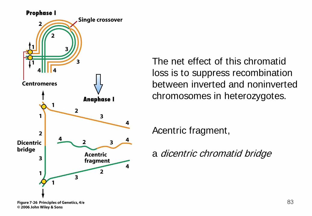
The net effect of this chromatid loss is to suppress recombination between inverted and noninverted chromosomes in heterozygotes. Acentric fragment, a dicentric chromatid bridge
83
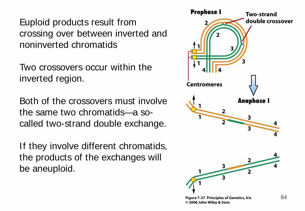
Euploid products result from crossing over between inverted and noninverted chromatids Two crossovers occur within the inverted region. Both of the crossovers must involve the same two chromatids—a so-called two-strand double exchange. If they involve different chromatids, the products of the exchanges will be aneuploid.
84

Geneticists have exploited the recombination-suppressing properties of inversions to keep alleles of different genes together on the same chromosome. Balancers: marked inversion chromosomes they allow a mutant chromosome to be kept in heterozygous condition over the inversion.
85
Genetic Control of Recombination Studies with several organisms, including yeast and Drosophila, have demonstrated that recombination involves the products of many genes. One curious phenomenon, which no one has yet explained, is that there is no crossing over in Drosophila males.
86