linking local extremes to atmospheric circulations › ~panja002 › acpd-7-14433-2007.pdf ·...

ACPD7, 14433–14460, 2007

Linking localextremes toatmosphericcirculations

D. Panja and F. M. Selten

Title Page

Abstract Introduction

Conclusions References

Tables Figures

J I

J I

Back Close

Full Screen / Esc

Printer-friendly Version

Interactive Discussion

EGU

Atmos. Chem. Phys. Discuss., 7, 14433–14460, 2007www.atmos-chem-phys-discuss.net/7/14433/2007/© Author(s) 2007. This work is licensedunder a Creative Commons License.

AtmosphericChemistry

and PhysicsDiscussions

Extreme associated functions: optimallylinking local extremes to large-scaleatmospheric circulation structuresD. Panja and F. M. Selten

Royal Netherlands Meteorological Institute (KNMI), Postbus 201, 3730 AE De Bilt, TheNetherlands

Received: 28 August 2007 – Accepted: 23 September 2007 – Published: 10 October 2007

Correspondence to: D. Panja ([email protected])

14433

http://www.atmos-chem-phys-discuss.net

http://www.atmos-chem-phys-discuss.net/7/14433/2007/acpd-7-14433-2007-print.pdf

http://www.atmos-chem-phys-discuss.net/7/14433/2007/acpd-7-14433-2007-discussion.html

http://www.egu.eu

ACPD7, 14433–14460, 2007



Title Page



Tables Figures

J I

J I

Back Close

Full Screen / Esc



EGU

Abstract

We present a new statistical method to optimally link local weather extremes to large-scale atmospheric circulation structures. The method is illustrated using July–Augustdaily mean temperature at 2 m height (T2m) time-series over the Netherlands and500 hPa geopotential height (Z500) time-series over the Euroatlantic region of the5

ECMWF reanalysis dataset (ERA40). The method identifies patterns in the Z500 time-series that optimally describe, in a precise mathematical sense, the relationship withlocal warm extremes in the Netherlands. Two patterns are identified; the most impor-tant one corresponds to a blocking high pressure system leading to subsidence andcalm, dry and sunny conditions over the Netherlands. The second one corresponds to10

a rare, easterly flow regime bringing warm, dry air into the region. The patterns arerobust; they are also identified in shorter subsamples of the total dataset. The methodis generally applicable and might prove useful in evaluating the performance of climatemodels in simulating local weather extremes.

1 Introduction15

Weather extremes such as extreme wind speeds, extreme precipitation or extremewarm or cold conditions are experienced locally. They are usually connected to circu-lation structures of much larger scale in the atmosphere. For example, if we restrictourselves to the Netherlands, a well-known circulation structure that often leads toextreme hot summer days is a high pressure system that blocks the inflow of cooler20

maritime air masses. Moreover, the subsidence of air in its interior leads to clear skiesand an abundance of sunshine that leads to high temperatures. If the blocking highpersists and depletes the soil moisture due to lack of precipitation and increased evap-oration, temperatures tend to soar, as it did in the European summer of 2003 Scharet al. (2004). Speculations about a positive feedback of dry soil on the persistence of25

the blocking high can also be found in the literature Ferranti and Viterbo (2006).

14434




http://www.egu.eu

ACPD7, 14433–14460, 2007



Title Page



Tables Figures

J I

J I

Back Close

Full Screen / Esc



EGU

In order for climate models to correctly simulate the probability of extreme hot sum-mer days, a crucial ingredient is the correct simulation of the probability of the occur-rence of blocking. This is a well-known difficult feature of the atmospheric circulationto simulate realistically Pelly and Hoskins (2003). The verification of models w.r.t. thisaspect is, in practice, difficult as well, since idealized model experiments suggest a5

high degree of internal variability of blocking frequencies even on decadal timescalesLiu and Opsteegh (1995).

In a world with increasing concentrations of greenhouse gases, not only thetemperature increases, also the large-scale circulation adjusts to achieve a new(thermo)dynamical balance. Models disagree on the magnitude and even the direc-10

tion of this change locally van Ulden and van Oldenborgh (2006). For instance, achange in the probability of European blocking conditions in summer immediately im-pacts the future probability of European heat waves. This makes probability estimatesof future European heat waves very uncertain. To address the questions concerningthe probability of future extreme weather events, and the evaluation of climate model15

simulations in this respect, it is necessary to have a descriptive method that links localweather extremes to large-scale circulation features. To the best of our knowledge, anoptimal method to do so does not exist in the literature.

We identified two approaches in the literature to link local weather extremes to large-scale circulation features. In the first one, the circulation anomalies are classified first,20

the connection with local extremes is analyzed in second instance. The “Grosswet-terlagen” developed by synoptic meteorologists for instance is one such classificationKysely (2002). All kinds of clustering algorithms are another example Plaut and Simon-net (2001); Cassou et al. (2005). In our opinion, this approach is not optimal since inthe definition of the patterns, information about the extreme is not taken into account.25

In the second approach, a measure of the local extreme does enter the definition ofthe large-scale circulation patterns. For instance, only atmospheric states are consid-ered for which the local extreme occurs. Next a simple averaging operator is applied(“composite method” as in Schaeffer et al., 2005) or a clustering analysis is performed

14435




http://www.egu.eu

ACPD7, 14433–14460, 2007



Title Page



Tables Figures

J I

J I

Back Close

Full Screen / Esc



EGU

Sanchez-Gomez and Terray (2005) . The composite method falls short since it finds bydefinition only one typical circulation anomaly and from synoptic experience we knowthat often different kind of circulation anomalies lead to a similar local weather extreme.The clustering analysis is debatable since the data record is often too short to identifyclusters with enough statistical confidence Hsu and Zwiers (2001).5

The purpose of this paper is to report a new optimal method to relate local weatherextremes to characteristic circulation patterns. This method objectively identifies, ina robust manner, the different circulation patterns that favor the occurrence of localweather extremes. The method is inspired by the Optimal Autocorrelation Functionsof Selten et al. (1999). It is based on considering linear combinations of the dominant10

Empirical Orthogonal Functions that maximize a suitable statistical quantity. We illus-trate our method by analyzing the statistical relation between extreme high daily meantemperatures at two meter height (T2m) in July and August in the Netherlands and thestructure of the large-scale circulation as measured by the 500 hPa geopotential heightfield (Z500).15

This paper is divided into five sections. Section 2 is focused on the data, wherewe explain the method to obtain the daily Z500 and T2m anomalies in Europe, andreport the results of the EOF analysis of the Z500 anomaly data. In Sect. 3 we outlinethe procedure to optimize the quantity that describes the statistical relation betweenthe Z500 and the extreme T2m anomalies, supported by the additional details in the20

Appendix. In Sect. 4 we identify the large-scale Z500 anomaly patterns that are as-sociated with hot summer days in the Netherlands, demonstrate the robustness of ourmethod and compare the patterns with patterns earlier reported in the literature. Finallywe conclude this report in Sect. 5 with a discussion on the possible applications of ourmethod.25

14436




http://www.egu.eu

ACPD7, 14433–14460, 2007



Title Page



Tables Figures

J I

J I

Back Close

Full Screen / Esc



EGU

2 The T2m and Z500 datasets, and EOF analysis of the Z500 data

Our data have been obtained from the ERA-40 reanalysis dataset, for the timespanSept. method to obtain the daily Z500 and 1957 to Aug. 2002, at 6 hourly intervals ona 2.5◦×2.5◦ latitude-longitude grid. These data are publicly available at the ECMWFwebsite http://data.ecmwf.int/data/d/era40 daily/. The T2m data over entire Europe,5

defined by 37.5◦ N–70◦ N and 10◦W–40◦ E, and the Z500 data over 20◦N–90◦ N and60◦ W–60◦ E were downloaded. From these, the daily averages for T2m and Z500fields for the years 1958–2000 (all together 43 years in total) were computed. Thisformed our full raw dataset.

In order to remove possible effects of global warming in the last decades of 20th10

century, detrending these fields prior to performing further calculations would be nec-essary. However, an analysis of the Z500 daily averaged field revealed no significantlinear trend over these 43 years. Therefore the Z500 daily anomaly field was obtainedby simply removing the seasonal cycle defined by an average over the entire periodof 43 years. Greatbatch and Rong (2006) showed that over Europe, the trends in the15

ERA-40 reanalysis and NCEP-NCAR reanalysis are indeed small and similar.A warming trend, however, is clearly present in the T2m field. For detrending the

T2m field, the monthly averages for July and August were calculated from the dailyaverages at each gridpoint. Next, 11-year running means were computed for thesemonthly averaged T2m fields (for July and August separately), and that formed our20

baseline for calculating daily T2m anomaly field. This procedure does not yield thebaseline for the first and the last 5 years (1958–1962 and 1996–2000); these werecomputed by extrapolating the baseline trend for the years 1963–1964 and 1995–1996respectively.

For the EOF analysis of the Z500 anomaly field, note that most of the variance25

of atmospheric variability resides in the low-frequency part (10–90 day range Maloneet al., 1984). Indeed, the dominant EOFs of Z500 anomaly fields proved insensitive tothe application of 3-day, 5-day, 7-day, 9-day and 15-day running mean filters. For the

14437




http://www.egu.eu

http://data.ecmwf.int/data/d/era40_daily/

ACPD7, 14433–14460, 2007



Title Page



Tables Figures

J I

J I

Back Close

Full Screen / Esc



EGU

sake of simplicity, therefore, we decided to only consider EOFs based on daily Z500anomaly fields. The EOF analysis was performed on the regular lat-lon grid data witheach grid point weighted by the cosine of its latitude to account for the different sizesof the grid cells. Using these weights, the EOFs ek are orthogonal in space (note herethat we use the same definition of vector dot product in space all throughout this paper.)5

ek · el≡1∑N

i=1 cos(φi )

N∑i=1

ek(λi , φi )el (λi , φi ) cos(φi )=δkl , (1)

where φ denotes latitude, λ longitude and N the total number of grid points, and δkl isthe Kronecker delta. Each Z500 anomaly field can be expressed in terms of the EOFsas

Z500(t)=N∑

k=1

ak(t)ek , (2)10

where the amplitudes ak are found by a projection of the Z500 anomaly on to the EOFs

ak(t)=Z500(t) · ek . (3)

A nice property of the EOFs is that their amplitude time-series are uncorrelated in timeat zero lag

〈ak(t)al (t)〉=σ2k δkl , (4)15

where the angular brackets 〈.〉 denote a time average and σ2k denotes the eigenvalue of

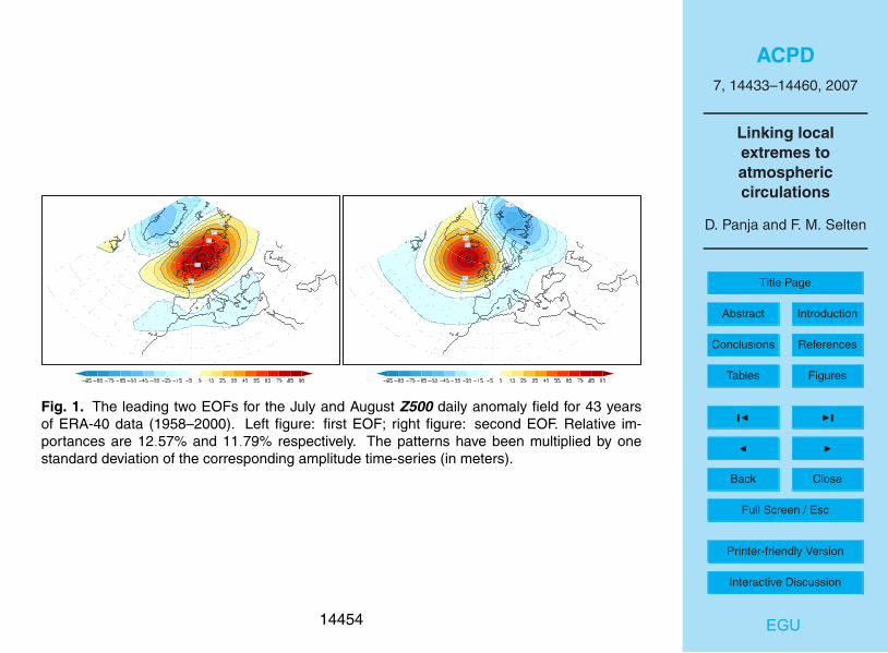
the k-th EOF which is equal to the variance of the corresponding amplitude time-series.We found that July and August months produced very similar EOFs, while June

and September EOFs were significantly different. We therefore decided to restrict thesummer months to July and August. The leading two EOFs for the corresponding20

daily Z500 anomaly for 1958–2000 are shown in Fig. 1. The values correspond toone standard deviation of the corresponding amplitude. The two EOFs are not well

14438




http://www.egu.eu

ACPD7, 14433–14460, 2007



Title Page



Tables Figures

J I

J I

Back Close

Full Screen / Esc



EGU

separated (the eigenvalues are close together) and therefore we expect some mixingbetween the two patterns North et al. (1982). A linear combination of the two EOFsshifts the longitudinal position of the strong anomaly over Southern Scandinavia whichis present in the first EOF. It resembles the summer NAO pattern as diagnosed byGreatbatch and Rong Greatbatch and Rong (2006) (their Fig. 8).5

3 Optimization procedure to establish the connection between Z500 anomaliesand local extreme T2m

One of the first approaches we considered to establish the connection between Z500daily anomaly fields and extreme daily T2m is the so-called “clustering method”, whichidentifies clusters of points in the vector space spanned by the dominant EOFs.10

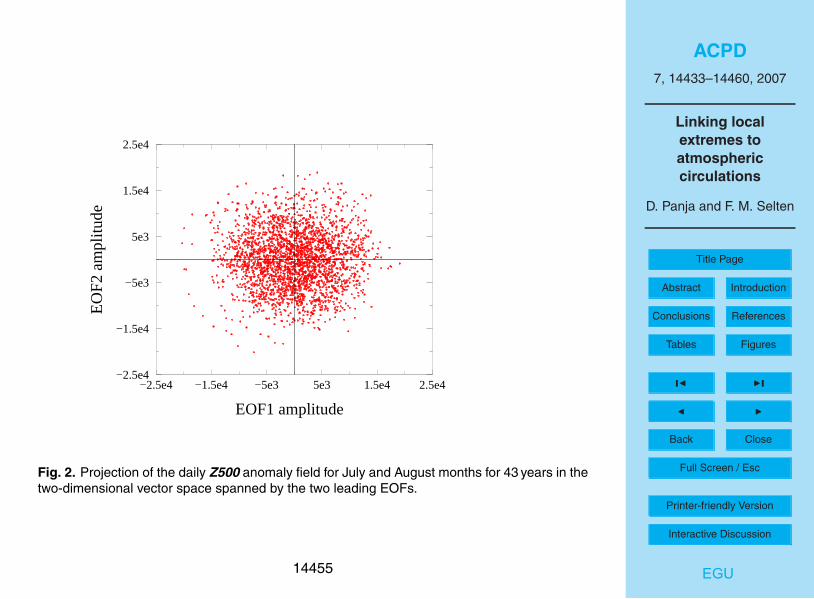
The daily Z500 anomaly field for July and August over 43 years yields us precisely2666 datapoints in this vector space. A projection of these daily anomalies on thetwo-dimensional vector space of the two leading EOFs (EOF1 and EOF2) is shown inFig. 2. No clear clusters are apparent by simple visual inspection. One can imaginethat defining clusters using existing cluster algorithms to identify clusters of points that15

correspond to specific large-scale circulation patterns that occur significantly more fre-quently than others is not a trivial undertaking. Often it turns out that using 40 years ofdata or so, the clusters identified are the result of sampling errors, due to too few datapoints Hsu and Zwiers (2001); Berner and Branstator (2007); Stephenson and O’Neill(2004).20

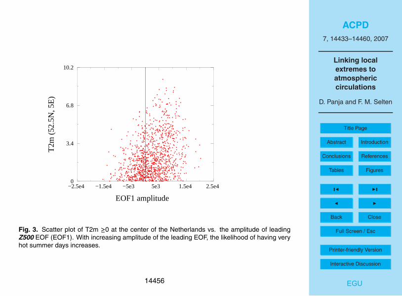
Nevertheless, when we plot the T2m positive anomaly values at the center of theNetherlands (52.5◦ N, 5◦ E) in a scatter plot with the amplitude of EOF1, a distinct “tilt”in the scatter plot emerges: i.e., with increasing amplitude of the leading EOF, thelikelihood of having very hot summer days increases. Having inspected the same plotsfor the other EOFs we found a similar tilt for some of the other EOFs as well. From25

this point of view, finding the statistical relationship between T2m at a given place andthe state of the large-scale atmospheric circulation can be reduced to a mathematical

14439




http://www.egu.eu

ACPD7, 14433–14460, 2007



Title Page



Tables Figures

J I

J I

Back Close

Full Screen / Esc



EGU

exercise that finds those linear combinations of EOFs that optimally bring out this tilt.In the remainder of this section, supported by the Appendix, we present a general,rigorous and robust procedure to achieve this.

To represent this statistical relationship, we start by defining the following dimension-less quantity5

r (L)k =

〈b(L)k (t) [T (t)]n〉p

〈[b(L)k (t)

]2〉

12p 〈[T (t)]n〉p

. (5)

Here the angular brackets 〈.〉p denotes a time average taken only over those days forwhich T2m(t)≥0, and n is a positive number >1. The idea behind choosing n>1 is thatfor higher T (t) it gives larger contribution to r (L)

k : we are interested in high-temperature

days at gridpoint G, we choose n=2 for this study. The variable b(L)k (t) is the amplitude10

on day t of a pattern, defined as a linear combination of the first L EOFs. Since L linearcombinations can be defined that form a new complete basis in the subspace of thefirst L EOFs we use the subscript k to denote these different linear combinations.

We first concentrate on the calculation of the first pattern. Using c(L)j1 to denote the

coefficients of this first linear combination then15

b(L)1 (t)=

L∑j=1

c(L)j1 aj (t) . (6)

Notice that since the time averages are taken only over those days for whichT2m(t) ≥ 0, 〈b(L)

1 (t)〉p 6= 0, although 〈b(L)1 (t)〉=0 since 〈aj (t)〉=0.

Equations (5–6) imply that given the time-series of T2m and Z500 anomalies, thenumerical value of r (L)

1 depends only on L and on the coefficients c(L)j1 . For a given20

value of L, c(L)j1 are found by maximizing the square of r (L)

1 within the vector space of

the first L EOFs (the square is taken since r (L)1 can take on negative values as well).

14440




http://www.egu.eu

ACPD7, 14433–14460, 2007



Title Page



Tables Figures

J I

J I

Back Close

Full Screen / Esc



EGU

If we define for T (t) ≥ 0,

Tp(t)=[T (t)]n

〈[T (t)]n〉p(7)

then Eq. (5) can be rewritten for k=1 as

r (L)1 =

〈b(L)1 (t) Tp(t)〉p

〈[b(L)

1 (t)]2〉

12p

. (8)

In words, maximizing[r (L)1

]2defines a pattern that for a change of one standard de-5

viation in its amplitude b1 brings about the largest change in the normalized positivetemperature anomaly Tp or put differently the local temperature responds most sensi-tively to changes in the normalized amplitude of this pattern. In this sense, the patternis optimally linked to the local warm temperature extremes.

It is shown in the Appendix that maximizing[r (L)1

]2corresponds to the linear least10

squares fit of the EOF amplitude timeseries to Tp(t)

T (L)p (t)=

L∑j=1

r (L)1 c(L)

j1 aj (t). (9)

with the coefficients cj1 given by

r (L)1 c(L)

j1 =L∑i=1

〈ai (t)aj (t)〉−1p 〈Tp(t)ai (t)〉p (10)

This result makes sense since the linear least squares fit optimally combines the15

EOF amplitude timeseries to minimize the mean squared error between the actual tem-perature anomaly and the temperature anomaly estimated from the circulation anomalyat that day.

14441




http://www.egu.eu

ACPD7, 14433–14460, 2007



Title Page



Tables Figures

J I

J I

Back Close

Full Screen / Esc



EGU

The procedure to find the remaining (L−1) linear combinations is as follows. Wefirst reduce the Z500 anomaly fields to the (L−1) dimensional subspace Z500(L−1) thatis orthogonal to the first linear combination. In this subspace we again determine thelinear combination that optimizes r (L)

2 . By construction, this value is lower than r (L)1 . This

procedure is repeated to determine all L linear combinations with decreasing order of5

optimized values r (L)k .

There is no unique way to define the subspaces and how this is done affects theproperties of the linear combinations. The linear combinations can either (a) be con-structed to form an orthonormal basis in space, in which case their amplitudes aretemporally correlated; or (b) they can be constructed so that the corresponding ampli-10

tudes are temporally uncorrelated, but in that case they are not orthonormal in space.In both cases, they form a complete basis in the space of the first L EOFs

Z500(L)(t)=L∑

k=1

b(L)k (t) f (L)

k . (11)

We will call the patterns f(L)k Extreme Associated Functions (EAFs). The mathemati-

cal details on how to obtain b(L)k (t) for both options can be found in the Appendix.15

4 Statistical relationship between high summer temperature in the Netherlandsand large-scale atmospheric circulation structures

We now need a criterion to determine the optimal number of EOFs in the linear com-binations. The reason for limiting the number of EOFs in the linear combinations isapparent from Eq. (10). Here the inverse of the covariance matrix of the EOF ampli-20

tudes appears. This matrix becomes close to singular when low-variance EOFs areincluded in the linear combination. This makes the solution for the coefficients c(L)

jkill-determined [see the general linear least squares section in Press et al. (1986) for a

14442




http://www.egu.eu

ACPD7, 14433–14460, 2007



Title Page



Tables Figures

J I

J I

Back Close

Full Screen / Esc



EGU

detailed discussion on this issue]. Typically what is observed is that the inclusion ofmany more low-variance EOFs only marginally improves the r (L)

k values, but that thecorresponding patterns describe less variance and become “noisier” i.e. project ontoZ500 variations at progressively smaller wavelengths. The optimal value of L in a sta-tistical procedure like this, denoted by Lc, is subjective, but nevertheless can be found5

from a tradeoff between the amount of variance that the patterns describe and theirr-values.

The procedure to determine Lc for the daily summer (July and August) temperaturein the Netherlands [represented by T2m at (52.5◦N,5◦E)] and Z500 daily anomaly fieldover the region 20◦N–90◦N and 60◦ W–60◦ E for 43 years (1958–2000) is as follows. As10

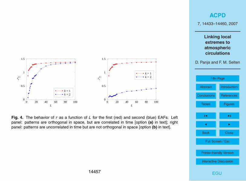
can be expected, both r (L)1 and r (L)

2 are increasing functions with L (Fig. 4 left) and thevariance associated with the corresponding EAFs tends to decrease with increasing L(not shown here). For option (a), both r (L)

1 and r (L)2 improve significantly when including

EOF12 in the linear combination; at the same time the variance of EAF1 decreases andthe variance of EAF2 increases. Also the corresponding patterns change markedly.15

Between L=12 and L=15 the patterns, r-values and variances remain relatively un-changed. Beyond L=15 the r-values steadily increase, the variance decreases andthe patterns become “noisier”. Simultaneously, the temporal correlation between thedominant two EAF patterns steadily increases with L. For large L, as Fig. 4(left) shows,both r (L)

1 and r (L)2 values saturate to values very close to each other, and the solution20

tends to become degenerate. Our interpretation of this is that the information that iscontained in the Z500 anomaly fields about the local temperatures in the Netherlandsis shared among increasingly more patterns, which is an undesirable characteristic.For example, for L=12, the temporal correlation between EAF1 and EAF2 is 0.58, forL=50 it is 0.93. Based on these findings, we consider Lc to be equal to 12.25

A similar graph for EAFs calculated following option (b) are also displayed inFig. 4(right). By construction, the value of r (L)

1 is the same. In this case, the variancedecreases as well with increasing L, but much less so. The corresponding patterns arequite stable beyond L=19. It is only beyond L=200 or so that the second EAF more

14443




http://www.egu.eu

ACPD7, 14433–14460, 2007



Title Page



Tables Figures

J I

J I

Back Close

Full Screen / Esc



EGU

and more resembles the first EAF; for L=19 the spatial correlation between EAF1 andEAF2 is only 0.2 (they are almost orthogonal), for L=200 it is 0.4 and for L=500 it is0.8. By construction, the temporal correlation between EAF1 and EAF2 remains zero.In this case, the choice of L is not so critical and we simply choose Lc=50.

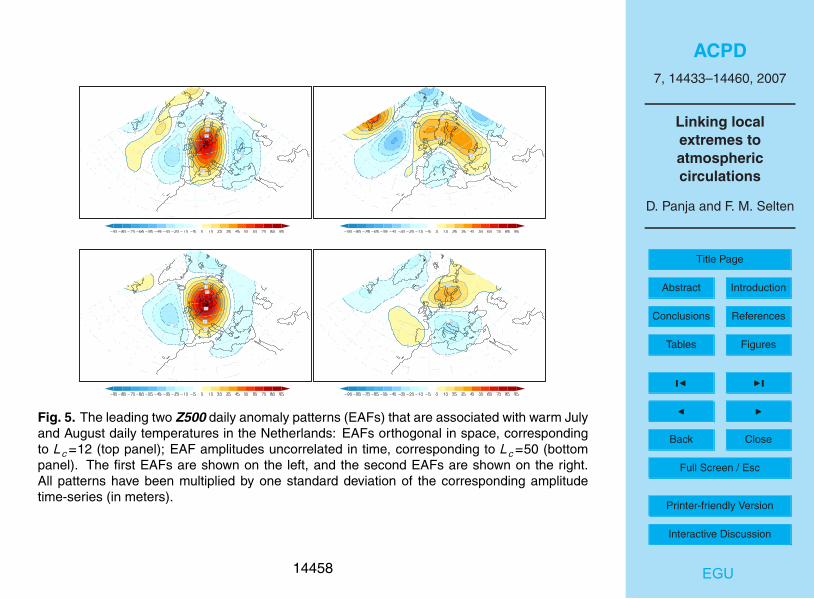
The results for the spatially orthogonal EAFs corresponding to Lc=12 and that for5

EAFs uncorrelated in time corresponding to Lc=50 are shown in Fig. 5. The first EAFsobtained from options (a) and (b) are very similar; the differences in the second arebigger. The first corresponds to a high pressure system, leading to clear skies over theNetherlands, an abundance of sunshine and a warm southeasterly flow. In addition tothis circulation anomaly, the method finds another pattern that occurs less often; EAF210

corresponds to an easterly flow regime bringing warm dry continental air masses to theNetherlands. Option (b) gives a more localized Z500 anomaly pattern, with a warm,easterly flow into the Netherlands. Option (a) also captures the warm, easterly flow,but is less localized and is less well defined as a function of L. The r (L)

2 value islarger for option (a), but it is temporally correlated to the first EAF. This implies that15

part of the information about the local warm temperatures in the Netherlands that iscontained in the amplitude timeseries of EAF2 is already captured by EAF1; they arenot independent. The r (L)

2 value is smaller for option (b), but at least the informationit contains about the local warm temperatures in the Netherlands is independent fromEAF1. Given these considerations, we conclude option (b), constructing EAFs that are20

temporally uncorrelated is the best option.

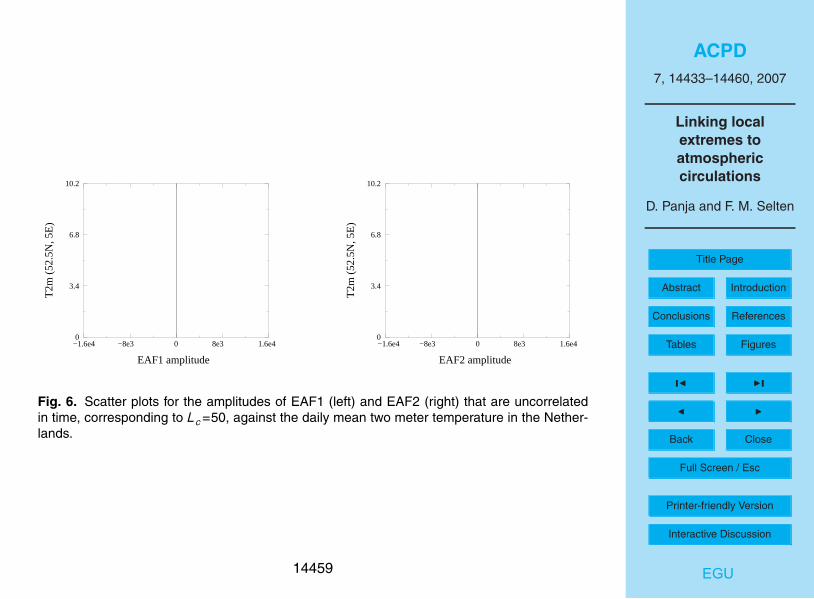
The scatterplots of b(Lc=50)1 and b

(Lc=50)2 against the positive temperature anomalies

in the Netherlands for EAF1 and EAF2 that are uncorrelated in time are shown in Fig. 6.Compared to the EOF with the largest r value (EOF1, see Fig. 3), the relationship of

b(Lc=50)1 to temperature is much stronger. The r value of the first EAF is almost a factor25

of 2 larger. The main contribution to the first EAF is from the first EOF, but also EOFs3,4 and 6 contribute substantially. Only two EAFs are found with a clear connection(i.e., a tilt in the scatterplot) to warm extremes in the Netherlands. This informationwas spread mainly between EOFs 1, 3, 4 and 6. Regressing Z500 anomalies upon the

14444




http://www.egu.eu

ACPD7, 14433–14460, 2007



Title Page



Tables Figures

J I

J I

Back Close

Full Screen / Esc



EGU

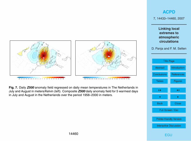
temperature time-series in the Bilt gives a pattern that resembles EAF1 (Fig. 7). Also asimple compositing (averaging the 5 percent hottest days) yields a pattern very similarto EAF1 (Fig. 7). In addition to this, the EAF method is able to identify another, lessdominant, flow configuration that leads to warm weather in the Netherlands throughadvection of warm airmasses from eastern Europe. Comparing EAF1 to the clusters5

of summer Z500 anomalies published in Cassou et al. (2005), we note that EAF1 is acombination of their “blocking” and “Atlantic low” regimes that favour warm conditionsin all of France and Belgium (temperatures in the Netherlands were not analyzed). Theeasterly flow regime is not present in their clusters.

In order to check that this method to identify the relevant large-scale atmospheric10

circulation patterns for warm days in the Netherlands is robust, we have also performedthe same analysis for the first 21 years (1958–1978) of daily summertime data and thelast 21 years (1980–2000). In both cases we found very similar EAF1 patterns andcorresponding scatter plots as for the full period. EAF2 however is only recovered inthe second period. One interpretation of this is that EAF2 is less frequently present in15

the first period. As argued by Liu and Opsteegh (1995) this variation could be entirelydue to the chaotic nature of the atmospheric circulation and need not be caused bya factor external to the atmosphere (as for instance increasing levels of greenhousegases, changes in sea surface temperatures or solar activity to name a few).

Instead of taking all positive temperature anomalies, a threshold could be introduced20

to Analise only the more extreme warm days. However, limiting the analysis to the30% warmest positive temperature anomalies did not qualitatively change the first twoEAFs. Also varying the value of the power applied to the temperature anomaly from1 to 3, only quantitatively modified the resulting EAFs, but not qualitatively. A finaltest of robustness was that we limited the analysis to a smaller domain. Again we25

found the same two EAF patterns on a much smaller domain from 20 degrees eastto 32.5 degrees west and 35 to 70 degrees north. The method thus produces robustpatterns.

14445




http://www.egu.eu

ACPD7, 14433–14460, 2007



Title Page



Tables Figures

J I

J I

Back Close

Full Screen / Esc



EGU

5 Discussion: applicability of the extreme associated functions

The Extreme Associated Function method developed in this study to establish the con-nection between local weather extremes and large-scale atmospheric circulation struc-tures has several potentially useful applications.

First of all, since this method proved to satisfy several tests of rigor and robustness5

for the temperature extremes in the Netherlands, it can be applied for local temperatureextremes at any other place, or for that matter for other forms of extreme local weatherconditions as well, like precipitation or wind. In this sense the method is quite general.

EAFs can be used to evaluate the performance of climate models with respect tothe occurrence of local weather extremes. The EAF method helps to answer the ques-10

tion whether the climate model is able to generate the same patterns that are foundin nature to be responsible for local weather extremes with a similar probability of oc-currence in an objective manner. In addition, to evaluate the impact of climate changeon local weather extremes, the EAF method helps to answer the question whether theprobability of certain local weather extremes changes in future scenario simulations15

due to a change in the probability of occurrence of the EAFs.It might be found that some climate models are able to simulate the EAFs, but do

not reproduce the local extremes well. Lenderink et al. (2007) for instance found thatregional climate models forced with the right large-scale circulation structures at thedomain boundaries nevertheless tended to overestimate the summer temperature vari-20

ability in Europe due to deficiencies in the description of the hydrological cycle. TheEAFs can be used to correct the model output for this discrepancy by applying the ob-served statistical relationship between the EAFs and the local extremes to the modelgenerated EAFs.

By choosing the particular form of r in Eq. (5) as the quantity to be optimized, the25

EAF method turns out to be equivalent to multiple linear regression. Other measures todescribe the statistical relationship between circulation and temperature present in thescatterplot of Fig. 3 could be designed that would make the EAF method different from

14446




http://www.egu.eu

ACPD7, 14433–14460, 2007



Title Page



Tables Figures

J I

J I

Back Close

Full Screen / Esc



EGU

a multiple linear regression technique. In this sense, the EAF method is more generaland potentially can be improved by designing a more apt measure.

Appendix A

Calculation of the EAFs by a repetitive maximization procedure5

Since the entire appendix describes the procedure to calculate b(L)k , i.e., the bk-values

for a given L, we drop all superscripts involving L for the sake of notational simplicity.

A1 Calculation of the first EAF

To calculate which set of coefficients cj1 maximize the value of r21 as expressed in

Eq. (8) we take the variation of r21 w.r.t. variations δcj1, and using Eq. (6), obtain10

δr21 =2×

L∑l=1

{〈T (t)ak(t)〉p〈T (t)al (t)〉p−[rmax

1 ]2〈ak(t)al (t)〉p}cl1δck1

〈[b(t)]2〉pfor k=1, . . . , L (A1)

This means that with the l.h.s. of Eq. (A1) set to zero at the maximum of r21 for

any choice of δck1, we obtain a generalized eigenvalue equation: if we denote〈T (t)ak(t)〉p〈T (t)al (t)〉p by ak al , and

[〈ak(t)al (t)〉p

]by v2

kl then Eq. (A1) leads to15

L∑l=1

{ak al − [rmax

1 ]2 v2kl

}cl1 =0 . (A2)

Equation (A2) can be written as a matrix equation

Ac1 =[rmax1 ]2 V2 c1, (A3)

14447




http://www.egu.eu

ACPD7, 14433–14460, 2007



Title Page



Tables Figures

J I

J I

Back Close

Full Screen / Esc



EGU

where the (k, l )-th element of matrices A and V2 are given by ak al and v2kl respectively,

and the l -th element of the column vector c1 is given by cl1. Note that in Eq. (A2)v2kl 6∝ δkl , since the time-average is defined only over the days for which T2m(t) ≥ 0.

Since matrix A is a tensor product of two column vectors A=aaT, where the superscript‘T’ indicates transpose, the matrix Eq. (A3) has only one eigenvector with non-zero5

eigenvalue, given by

c1 ∝ V−2a. (A4)

or equivalently

cj1 ∝L∑i=1

〈ai (t)aj (t)〉−1p 〈Tp(t)ai (t)〉p. (A5)

The corresponding optimized value r1 is determined from Eq. (A3).10

The equivalence between the maximization of r21 and the multiple linear regression

of Tp(t) on the timeseries of the EOF amplitudes ak(t)’s (see Eq. 9) is apparent bynoticing that the above solution for c1 is the same as the solution of the multiple linearregression problem given in Eq. (10).

How the EAFs are determined from the coefficients cjk is shown in the next section15

in which we explain the calculation of the remaining (L−1) EAFs.

A2 Calculation of the remaining (L−1) EAFs

As explained in the text, the calculation of the remaining (L−1) linear combinationsrequires a choice between two options. (a) The patterns are orthogonal in space, or,(b) the amplitude timeseries are uncorrelated in time. We will show the implementation20

of both options.We first discuss option (a).

14448




http://www.egu.eu

ACPD7, 14433–14460, 2007



Title Page



Tables Figures

J I

J I

Back Close

Full Screen / Esc



EGU

Combining the expansion of Z500(t) into EOFs as in Eq. (2) and into EAFs as inEq. (11) gives the following relation between the EOFs and EAFs

ei=L∑

k=1

cik fk for i=1, . . . , L (A6)

Option (a) demands the EAFs to be orthonormal in space which leads to the followingcondition for the corresponding coefficients cjk where we start from the orthonormality5

condition of the EOFs

ei · ej=L∑

k,l=1

cik cj l fk · f l=L∑

k=1

cik cjk=δi j . (A7)

Additionally, it can be easily shown thatL∑i=1

cik ci l=δkl . (A8)

Using Eq. (A8), it is now straightforward to show from Eq. (A6) that the EAFs can be10

calculated from the EOFs as

fk=L∑i=1

cik ei for k=1, . . . , L. (A9)

Using this definition for the EAFs, the corresponding amplitudes bk(t) are found by

bk(t)=fk · Z500(t). (A10)

We now discuss option (b).15

For option (b), Eqs. (11) and (A10) cannot hold simultaneously. To obtain the coeffi-cients ci j for this option, we start with Eq. (11) and define

bk(t)=L∑i=1

cik ai (t)=L∑i=1

cik ek · Z500(t)≡gk · Z500(t) (A11)

14449




http://www.egu.eu

ACPD7, 14433–14460, 2007



Title Page



Tables Figures

J I

J I

Back Close

Full Screen / Esc



EGU

Then the conditions that bk(t) and bl (t) are uncorrelated in time, i.e.,

〈bk(t)bl (t)〉=δkl (A12)

yields, using the fact that the EOF amplitudes are uncorrelated in time,

L∑i ,j

cik〈ai (t)aj (t)〉cj l=L∑i

cik σ2i ci l=δkl . (A13)

We then define5

fk=L∑i=1

cik σ2i ei for k=1, . . . , L (A14)

in terms of which Eq. (A12) can be re-expressed as

fk · gl=δkl . (A15)

Note here that for option (a) the patterns fk are automatically normalized to unity.For option (b), the patterns fk can be normalized to one, but the normalization of gk10

should be adjusted as well in order for Eq. (A15) to remain valid.To obtain the rest of the (L−1) EAFs, the procedure described in Appendix A1 needs

to be repeated L−1 times, but certain care needs to be taken because of the orthonor-mality condition imposed by the definition of the set of EAFs. When these subtle issuesare taken into account, the procedure becomes a repetition of the following three steps.15

(i) Construct Z500′(t), the Z500 daily anomaly field that lies within the vector sub-space of the first L EOFs but orthogonal to the first EAF. This is achieved in thefollowing manner.

First define

e′j=ej − (ej · f1) f1=ej − cj1 f1 (A16)20

14450




http://www.egu.eu

ACPD7, 14433–14460, 2007



Title Page



Tables Figures

J I

J I

Back Close

Full Screen / Esc



EGU

for j=2, . . . , L. The dot product of both sides of Eq. (A16) with Z500(t) then yields

a′j (t)=aj (t) − cj1 b1(t) for j=2, . . . , L (A17)

for option (a). For option (b), the corresponding expression is

a′j (t)=aj (t) − cj1 σ2j b1(t) for j=2, . . . , L. (A18)

(ii) Calculate the coefficients c′j2 for j=2, . . . , L that maximize r2.5

r2c′j2=

L∑i=1

〈a′i (t)a′j (t)〉

−1p 〈Tp(t)a′i (t)〉p (A19)

with

b2(t)=L∑

j=2

c′j2 a

′j (t) ≡

L∑j=1

cj2 a2(t). (A20)

(iii) Next the coefficients cj2 are calculated from the coefficients c′j2. For option (a)

substitution of Eq. (A17) into Eq. (A20) leads to10

cj2=c′j2 − cj1

L∑i=1

c′i2 ci1 for j=2, . . . , L, (A21)

with the convention that c′12=0. For option (b) substitution of Eq. (A18) into

Eq. (A20) leads to

cj2=c′j2 − cj1

L∑i=1

c′i2 σ

2i ci1 for j=2, . . . , L, (A22)

14451




http://www.egu.eu

ACPD7, 14433–14460, 2007



Title Page



Tables Figures

J I

J I

Back Close

Full Screen / Esc



EGU

with the convention that c′12=0.

These steps are to be repeated until all L coefficient vectors have been deter-mined. For option (a) the EAFs are then determined from Eq. (A9), for option (b)from Eq. (A14).

Acknowledgements. We thank ECMWF for making the Z500 data publicly available. We also5

acknowledge the ENSEMBLES project, funded by the European Commission’s 6th FrameworkProgramme through contract GOCE-CT-2003-505539.

References

Berner, J. and Branstator, G.: Linear and nonlinear signatures in the planetary wave dynamicsof an agcm: probability densitiy functions, J. Atmos. Sci., 64, 117–136, 2007. 1443910

Cassou, C., Terray, L., and Phillips, A.: Tropical Atlantic influence on European heat waves, J.Climate, 18, 2805–2811, 2005. 14435, 14445

D. Stephenson, A. H. and O’Neill, A.: On the existence of multiple climate regimes, Quart. J.Roy. Meteor. Soc., 130, 583–605, 2004. 14439

Ferranti, L. and Viterbo, P.: The European summer of 2003: sensitivity to soil water initial15

conditions, J. Climate, 19, 3659–3680, 2006. 14434Greatbatch, R. and Rong, P. P.: Discrepancies between different northern hemisphere summer

atmospheric data products, J. Climate, 19, 1261–1273, 2006. 14439Hsu, C. J. and Zwiers, F.: Climate change in recurrent regimes and modes of northern hemi-

sphere atmospheric variability, J. Geophys. Res., 106, 20 145–20 159, 2001. 14436, 1443920

Kysely, J.: Temporal fluctuations in heat waves at Prague-Klementinum, the Czech Republic,from 1901–97, and their realationships to atmospheric circulation, Int. J. Climatol., 22, 33–50,2002. 14435

Lenderink, G., van Ulden A., van den Hurk B., et al.: Summertime inter-annual temperaturevariability in an ensemble of regional model simulations: analysis of the surface energy25

budget, Climatic Change, 81, 233–247, 2007. 14446Liu, Q. and Opsteegh, J.: Interannual and decadal varations of blocking activity in a quasi-

geostrophic model, Tellus, 47A, 941–954, 1995. 14435, 14445

14452




http://www.egu.eu

ACPD7, 14433–14460, 2007



Title Page



Tables Figures

J I

J I

Back Close

Full Screen / Esc



EGU

Malone, R., Pitcher E. J., Blackmon, M. L., et al.: The simulation of stationary and transientgeopotential-height eddies in January and July with a spectral general circulation model, J.Atmos. Sci., 41, 1394–1419, 1984. 14437

North, G., Bell, T. L., Calahan, R. F., et al.: Sampling errors in the estimation of empiricalorthogonal functions, Mon. Weather Rev., 110, 699–706, 1982. 144395

Pelly, J. L. and Hoskins, B. J.: How well does the ECMWF ensemble prediction system predictblocking?, Q. J. R. Meteorol. Soc., 129, 1683–1702, 2003. 14435

Plaut, G. and Simonnet, E.: Large-scale circulation classification weather regimes, and locallcimate over France, the Alps and Western Europe, Clim. Res., 17, 303–324, 2001. 14435

Press, W. H., Flannery, B. P., Teukolsky, S. A. and Vetterling, W. T.: Numerical Recipes, Cam-10

bridge University Press, isbn 0521308119, 818pp, 1986. 14442Sanchez-Gomez, E. and Terray, L.: Large-scale atmospheric dynamics and local intense pre-

cipitation episodes, Geophys. Res. Lett., 32, L2471, 2005. 14436Schaeffer, M., Selten, F. M., and Opsteegh, J. D.: Shifts of means are not a proxy for changes

in extreme winter temperatures in climate projections, Clim. Dyn., 25, 51–63, 2005. 1443515

Schar, C., Vidale, P. L., Luthi, D., et al.: The role of increasing temperature variability in Euro-pean summer heat waves, Nature, 427, 332–336, 2004. 14434

Selten, F., Haarsma, R., and Opsteegh, J.: On the mechanism of north Atlantic decadal vari-ability, J. Climate, 12, 1256–1973, 1999. 14436

van Ulden, A. and van Oldenborgh, G.: Large-scale atmospheric circulation biases and20

changes in global climate model simulations and their importance for climate change in Cen-tral Europe, Atmos. Chem. Phys., 6, 863–881, 2006,http://www.atmos-chem-phys.net/6/863/2006/. 14435

14453




http://www.egu.eu

http://www.atmos-chem-phys.net/6/863/2006/

ACPD7, 14433–14460, 2007



Title Page



Tables Figures

J I

J I

Back Close

Full Screen / Esc



EGU

Fig. 1. The leading two EOFs for the July and August Z500 daily anomaly field for 43 yearsof ERA-40 data (1958–2000). Left figure: first EOF; right figure: second EOF. Relative im-portances are 12.57% and 11.79% respectively. The patterns have been multiplied by onestandard deviation of the corresponding amplitude time-series (in meters).

14454




http://www.egu.eu

ACPD7, 14433–14460, 2007



Title Page



Tables Figures

J I

J I

Back Close

Full Screen / Esc



EGU

−2.5e4 −1.5e4 −5e3 5e3 1.5e4 2.5e4

EOF1 amplitude

−2.5e4

−1.5e4

−5e3

5e3

1.5e4

2.5e4

EO

F2 a

mpl

itude

Fig. 2. Projection of the daily Z500 anomaly field for July and August months for 43 years in thetwo-dimensional vector space spanned by the two leading EOFs.

14455




http://www.egu.eu

ACPD7, 14433–14460, 2007



Title Page



Tables Figures

J I

J I

Back Close

Full Screen / Esc



EGU

−2.5e4 −1.5e4 −5e3 5e3 1.5e4 2.5e4

EOF1 amplitude

0

3.4

6.8

10.2

T2m

(52

.5N

, 5E

)

Fig. 3. Scatter plot of T2m ≥0 at the center of the Netherlands vs. the amplitude of leadingZ500 EOF (EOF1). With increasing amplitude of the leading EOF, the likelihood of having veryhot summer days increases.

14456




http://www.egu.eu

ACPD7, 14433–14460, 2007



Title Page



Tables Figures

J I

J I

Back Close

Full Screen / Esc



EGU

0 20 40 60 80 100L

0

0.5

1

1.5

r(L)

k

k = 1k = 2

0 20 40 60 80 100L

0

0.5

1

1.5

r(L)

k

k = 1k = 2

Fig. 4. The behavior of r as a function of L for the first (red) and second (blue) EAFs. Leftpanel: patterns are orthogonal in space, but are correlated in time [option (a) in text]; rightpanel: patterns are uncorrelated in time but are not orthogonal in space [option (b) in text].

14457




http://www.egu.eu

ACPD7, 14433–14460, 2007



Title Page



Tables Figures

J I

J I

Back Close

Full Screen / Esc



EGU

Fig. 5. The leading two Z500 daily anomaly patterns (EAFs) that are associated with warm Julyand August daily temperatures in the Netherlands: EAFs orthogonal in space, correspondingto Lc=12 (top panel); EAF amplitudes uncorrelated in time, corresponding to Lc=50 (bottompanel). The first EAFs are shown on the left, and the second EAFs are shown on the right.All patterns have been multiplied by one standard deviation of the corresponding amplitudetime-series (in meters).

14458




http://www.egu.eu

ACPD7, 14433–14460, 2007



Title Page



Tables Figures

J I

J I

Back Close

Full Screen / Esc



EGU

−1.6e4 −8e3 0 8e3 1.6e4

EAF1 amplitude

0

3.4

6.8

10.2

T2m

(52

.5N

, 5E

)

−1.6e4 −8e3 0 8e3 1.6e4

EAF2 amplitude

0

3.4

6.8

10.2

T2m

(52

.5N

, 5E

)

Fig. 6. Scatter plots for the amplitudes of EAF1 (left) and EAF2 (right) that are uncorrelatedin time, corresponding to Lc=50, against the daily mean two meter temperature in the Nether-lands.

14459




http://www.egu.eu

ACPD7, 14433–14460, 2007



Title Page



Tables Figures

J I

J I

Back Close

Full Screen / Esc



EGU

Fig. 7. Daily Z500 anomaly field regressed on daily mean temperatures in The Netherlands inJuly and August in meters/Kelvin (left). Composite Z500 daily anomaly field for 5 warmest daysin July and August in the Netherlands over the period 1958–2000 in meters.

14460




http://www.egu.eu

linking local extremes to atmospheric circulations › ~panja002 › acpd-7-14433-2007.pdf ·...

Documents