lin/operations/supply chain mgt1 supply chain management module u managing the supply chain »key to...

Lin/Operations/Supply Chain Mgt 1

Supply Chain Management Module Managing the Supply Chain

» Key to matching demand with supply» Cost and Benefits of inventory

Economies of Scale» Palu Gear: Inventory management of a retailer: EOQ + ROP » Levers for improvement

Safety Stock» Hedging against uncertainty» Role of leadtime

Improving Performance» Centralization & Pooling efficiencies» Postponement» Optimal Service Level


What is a Supply Chain?

What makes for a “good” SC?

Raw Materialsupply points

Movement/Transport

Raw MaterialStorage Movement/

TransportMovement/Transport

PLANT 1

PLANT 2

PLANT 3

WAREHOUSES(DCs)

Movement/Transport

MARKETS

Manufacturing

Finished GoodsStorage

A

B

C

1. Procurementor supply system

2. OperatingSystem 3. Distribution System

4. Salesor demand system


US Vehicle Inventory


Corporate Finance

Inventories represent about 34% of current assets for a typical US company; 90% of working capital.

For each dollar of GNP in the trade and manufacturing sector, about 40% worth of inventory was held.

Average logistics cost = 21¢/sales dollar = 10.5% of GDP

Cisco SolectronCurrent Assets 7/30/95 8/25/95Cash & Equivalents 204,846 21% 89,959 12%Short-term Investments 234,681 58,643 AR 384,242 254,898 Inventories 71,160 7% 298,809 41%Deferred income taxes 75,297other 25,743 24,049 Total current assets 995,969 100% 726,358 100%

Investments 576,958PPE 136,653 203,609 other 47747 10,888 Total assets 1,757,327 940,855


Costs of not Matching Supply and Demand

Cost of overstocking – liquidation, obsolescence, holding

Cost of under-stocking – lost sales and resulting lost margin


We never Talk anymore!

In Style

People

Vanity Fair

Vogue

The New Yorker

GQ

New York

Esquire

Rolling Stone

Us

Talk

64.7%

54.5%

45.6%

42.1%

39.9%

39.4%

35.1%

31.0%

28.0%

23.9%

18.0%

Data for Oct. 1999 – Oct. 2000

Magazine sales at newsstands as % of copies shipped to newsstands


The Current Environment:The Grocery Industry 1985-1992

Number of products in average supermarket

1985 11,036

1990 16,486

1992 20,000

2004 ??

1975 1992 2002

2,000

20,000


A Key to Matching Supply and Demand

When would you rather place your bet?

A B C D

A: A month before start of DerbyB: The Monday before start of DerbyC: The morning of start of DerbyD: The winner is an inch from the finish line


Where is the Flow Time?

Buffer Operation

Waiting Processing


Operational Flows

Throughput R

Inventory I

I = R T Flow time T = Inventory I / Throughput R

FLOW TIME T


Why do Buffers Build?Why hold Inventory?

Economies of scale– Fixed costs associated with batches

– Quantity discounts

– Trade Promotions

Uncertainty– Information Uncertainty

– Supply/demand uncertainty

Seasonal Variability Strategic

– Flooding, availability

Cycle/Batch stock

Safety stock

Seasonal stock

Strategic stock


Annual jacket revenues at a Palü Gear retail store are roughly $1M. Palü jackets sell at an average retail price of $325, which represents a mark-up of 30% above what Palü Gear paid its manufacturer. Being a profit center, each store made its own inventory decisions and was supplied directly from the manufacturer by truck. A shipment up to a full truck load, which was about 3000 jackets, was charged a flat fee of $2,200. Typically, stores placed roughly two orders per year, each of about 1500 jackets. (Palü’s cost of capital is approximately 20%.)

What order size would you recommend for a Palü store in current supply network?

retailermanufacturer

Palü Gear: Retail Inventory Management & Economies of Scale


Economies of Scale: Inventory Build-Up Diagram

R: Annual demand rate,

Q: Number of jackets per replenishment order

Number of orders per year = R/Q.

Average number of jackets in inventory = Q/2 .

Q

Time t

Inventory Profile:# of wind breakers in inventory over time.

R = Demand rate

Inventory


Palü Gear: evaluation of current policy of ordering Q = 1500 units each time1. What is average inventory I?

I = Q/2 = Annual cost to hold one unit H = Annual cost to hold I = Holding cost × Inventory

2. How often do we order? Annual throughput R = # of orders per year = Throughput / Batch size Annual order cost = Order cost × # of orders

3. What is total cost? TC = Annual holding cost + Annual order cost =

4. What happens if order size changes?


Find most economical order quantity: Spreadsheet for a Palü Gear retailer

Number of units Number ofper order/batch Batches per Annual Annual Annual

Q Year: R/Q Setup Cost Holding Cost Total Cost50 62 135,385$ 1,250$ 136,635$ 100 31 67,692$ 2,500$ 70,192$ 150 21 45,128$ 3,750$ 48,878$ 200 15 33,846$ 5,000$ 38,846$ 250 12 27,077$ 6,250$ 33,327$ 300 10 22,564$ 7,500$ 30,064$ 350 9 19,341$ 8,750$ 28,091$ 400 8 16,923$ 10,000$ 26,923$ 450 7 15,043$ 11,250$ 26,293$ 500 6 13,538$ 12,500$ 26,038$ 510 6 13,273$ 12,750$ 26,023$ 520 6 13,018$ 13,000$ 26,018$ 530 6 12,772$ 13,250$ 26,022$ 540 6 12,536$ 13,500$ 26,036$ 550 6 12,308$ 13,750$ 26,058$ 600 5 11,282$ 15,000$ 26,282$ 650 5 10,414$ 16,250$ 26,664$ 700 4 9,670$ 17,500$ 27,170$ 750 4 9,026$ 18,750$ 27,776$ 800 4 8,462$ 20,000$ 28,462$ 850 4 7,964$ 21,250$ 29,214$ 900 3 7,521$ 22,500$ 30,021$

1000 3 6,769$ 25,000$ 31,769$

$-

$20,000

$40,000

$60,000

$80,000

$100,000

$120,000

$140,000

$160,000

0 100 200 300 400 500 600 700 800 900 1000

Order (batch) size Q

Setup Cost

Holding Cost

Total Cost


Economies of Scale: Economic Order Quantity EOQ

R : Demand per year,

S : Setup or Order Cost ($/setup; $/order),

H : Marginal annual holding cost ($ per unit per year),

Q : Order quantity.

C : Cost per unit ($/unit),

r : Cost of capital (%/yr),

H = r C.

H

SRQEOQ

2

Batch Size Q

Total annual costs

H Q/2: Annual holding cost

S R /Q:Annual setup cost

EOQ

SRH2


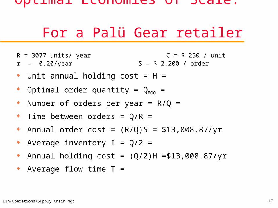
Optimal Economies of Scale: For a Palü Gear retailer

R = 3077 units/ year C = $ 250 / unitr = 0.20/year S = $ 2,200 / order

Unit annual holding cost = H =

Optimal order quantity = QEOQ =

Number of orders per year = R/Q =

Time between orders = Q/R =

Annual order cost = (R/Q)S = $13,008.87/yr

Average inventory I = Q/2 =

Annual holding cost = (Q/2)H =$13,008.87/yr

Average flow time T =


Role of Leadtime L: Palü Gear cont.

The lead time from when a Palü Gear retailer places an order to when the order is received is two weeks. If demand is stable as before, when should the retailer place an order?

I-Diagram:

The two key decisions in inventory management are:– How much to order?– When to order?


Learning Objectives: Batching & Economies of Scale

Increasing batch size of production (or purchase) increases average inventories (and thus cycle times).

Average inventory for a batch size of Q is Q/2. The optimal batch size trades off setup cost and holding cost. To reduce batch size, one has to reduce setup cost (time). Square-root relationship between Q and (R, S):

– If demand increases by a factor of 4, it is optimal to increase batch size by a factor of 2 and produce (order) twice as often.

– If demand increases by a factor of 4, the flow time decreases by a factor of 2.

An inventory policy must specify when to order (the ROP) and how much to order (the batch size).


Demand uncertainty and forecasting

Year Demand1992 194

1993 251

1994 320

1995 267

1995 233

1997 223

1998 266

1999 252

2000 251

2001 331


Demand uncertainty and forecasting

Forecasts depend on (a) historical data and (b) “market intelligence.”

Forecasts are usually (always?) wrong. A good forecast has at least 2 numbers (includes a

measure of forecast error, e.g., standard deviation). The forecast horizon must at least be as large as the

lead time. The longer the forecast horizon, the less accurate the forecast.

Aggregate forecasts tend to be more accurate.


Palü Gear:Service levels & inventory management

In reality, a Palü Gear store’s demand fluctuates from week to week. In fact, weekly demand at each store had a standard deviation of about 30 jackets assume roughly normally distributed. Recall that average weekly demand was about 59 jackets; the order lead time is two weeks; fixed order costs are $2,200/order and it costs $50 to hold one jacket in inventory during one year.

Questions: 1. If the retailer uses the ordering policy discussed before, what will the probability

of running out of stock in a given cycle be?

2. The Palü retailer would like the stock-out probability to be smaller. How can she accomplish this?

3. Specifically, how does it get the service level up to 95%?


Applications: – Demand over the leadtime L has standard deviation = RL – Pooled demand over N regions or products has standard deviation = RN

R R R…

Sum of N independent random variables, each with identical standard deviation Rhas

standard deviation =

How find of lead time demand?


Example: say we increase ROP to 140 (and keep order size at Q = 520)1. On average, what is the stock level when the replenishment arrives? 2. On average, what is the inventory profile?

3. What is the probability that we run out of stock?

4. How do we get that stock-out probability down to 5%?

0

100

200

300

400

500


Safety Stocks

Q

Time t

ROP

L

R

L

order order order

mean demand during supply lead time:

= R L

safety stock Is

Inventory on hand

I(t)

Q

Is

0

L


Safety Stocks & Service Levels: The relationship

Raise ROP until we reach appropriate SL

To do numbers, we need: Mean and stdev of demand during lead time Either Excel or tables with z - value such that CSL = F(z)

mean ROP

F(z)

demand during supply lead time

Stock-out probability

Cycle Service Level (CSL)

Is = z


1. How to find service level (given ROP)?2. How to find re-order point (given SL)?

L = Supply lead time, D =N(RR) = Demand per unit time is normally distributed

with mean R and standard deviation R ,

DL =N(LL) = Demand during the lead time

where L = RL and LRL

1. Given ROP, find SL = Cycle service level = P(no stock out)

= P(demand during lead time < ROP)

= F(z*= (ROP- L)/L) [use table]

= NORMDIST(ROP, L, L, True) [or Excel]

2. Given SL, find ROP = L + Is

= L + z*L[use table to get z* ]

= NORMINV(SL, L, L) [or Excel]

Safety stock Is = z*L Reorder point ROP = L + Is


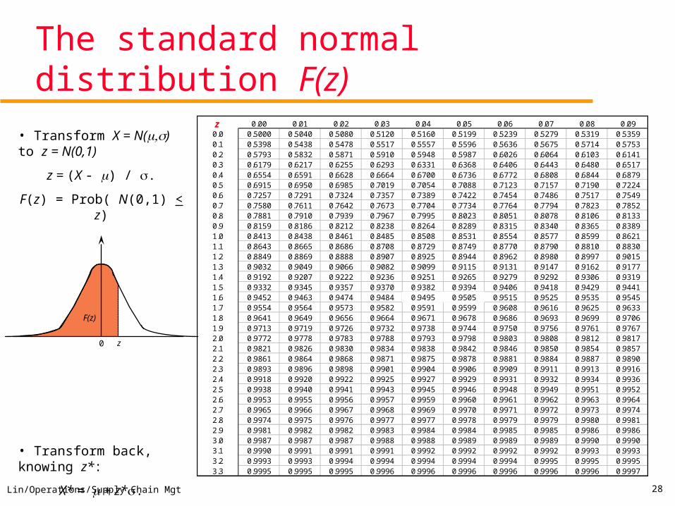
The standard normal distribution F(z)z 0.00 0.01 0.02 0.03 0.04 0.05 0.06 0.07 0.08 0.09

0.0 0.5000 0.5040 0.5080 0.5120 0.5160 0.5199 0.5239 0.5279 0.5319 0.53590.1 0.5398 0.5438 0.5478 0.5517 0.5557 0.5596 0.5636 0.5675 0.5714 0.57530.2 0.5793 0.5832 0.5871 0.5910 0.5948 0.5987 0.6026 0.6064 0.6103 0.61410.3 0.6179 0.6217 0.6255 0.6293 0.6331 0.6368 0.6406 0.6443 0.6480 0.65170.4 0.6554 0.6591 0.6628 0.6664 0.6700 0.6736 0.6772 0.6808 0.6844 0.68790.5 0.6915 0.6950 0.6985 0.7019 0.7054 0.7088 0.7123 0.7157 0.7190 0.72240.6 0.7257 0.7291 0.7324 0.7357 0.7389 0.7422 0.7454 0.7486 0.7517 0.75490.7 0.7580 0.7611 0.7642 0.7673 0.7704 0.7734 0.7764 0.7794 0.7823 0.78520.8 0.7881 0.7910 0.7939 0.7967 0.7995 0.8023 0.8051 0.8078 0.8106 0.81330.9 0.8159 0.8186 0.8212 0.8238 0.8264 0.8289 0.8315 0.8340 0.8365 0.83891.0 0.8413 0.8438 0.8461 0.8485 0.8508 0.8531 0.8554 0.8577 0.8599 0.86211.1 0.8643 0.8665 0.8686 0.8708 0.8729 0.8749 0.8770 0.8790 0.8810 0.88301.2 0.8849 0.8869 0.8888 0.8907 0.8925 0.8944 0.8962 0.8980 0.8997 0.90151.3 0.9032 0.9049 0.9066 0.9082 0.9099 0.9115 0.9131 0.9147 0.9162 0.91771.4 0.9192 0.9207 0.9222 0.9236 0.9251 0.9265 0.9279 0.9292 0.9306 0.93191.5 0.9332 0.9345 0.9357 0.9370 0.9382 0.9394 0.9406 0.9418 0.9429 0.94411.6 0.9452 0.9463 0.9474 0.9484 0.9495 0.9505 0.9515 0.9525 0.9535 0.95451.7 0.9554 0.9564 0.9573 0.9582 0.9591 0.9599 0.9608 0.9616 0.9625 0.96331.8 0.9641 0.9649 0.9656 0.9664 0.9671 0.9678 0.9686 0.9693 0.9699 0.97061.9 0.9713 0.9719 0.9726 0.9732 0.9738 0.9744 0.9750 0.9756 0.9761 0.97672.0 0.9772 0.9778 0.9783 0.9788 0.9793 0.9798 0.9803 0.9808 0.9812 0.98172.1 0.9821 0.9826 0.9830 0.9834 0.9838 0.9842 0.9846 0.9850 0.9854 0.98572.2 0.9861 0.9864 0.9868 0.9871 0.9875 0.9878 0.9881 0.9884 0.9887 0.98902.3 0.9893 0.9896 0.9898 0.9901 0.9904 0.9906 0.9909 0.9911 0.9913 0.99162.4 0.9918 0.9920 0.9922 0.9925 0.9927 0.9929 0.9931 0.9932 0.9934 0.99362.5 0.9938 0.9940 0.9941 0.9943 0.9945 0.9946 0.9948 0.9949 0.9951 0.99522.6 0.9953 0.9955 0.9956 0.9957 0.9959 0.9960 0.9961 0.9962 0.9963 0.99642.7 0.9965 0.9966 0.9967 0.9968 0.9969 0.9970 0.9971 0.9972 0.9973 0.99742.8 0.9974 0.9975 0.9976 0.9977 0.9977 0.9978 0.9979 0.9979 0.9980 0.99812.9 0.9981 0.9982 0.9982 0.9983 0.9984 0.9984 0.9985 0.9985 0.9986 0.99863.0 0.9987 0.9987 0.9987 0.9988 0.9988 0.9989 0.9989 0.9989 0.9990 0.99903.1 0.9990 0.9991 0.9991 0.9991 0.9992 0.9992 0.9992 0.9992 0.9993 0.99933.2 0.9993 0.9993 0.9994 0.9994 0.9994 0.9994 0.9994 0.9995 0.9995 0.99953.3 0.9995 0.9995 0.9995 0.9996 0.9996 0.9996 0.9996 0.9996 0.9996 0.9997

F(z)

z0

• Transform X = N() to z = N(0,1)

z = (X - ) / .

F(z) = Prob( N(0,1) < z)

• Transform back, knowing z*:

X* = + z*.


Palü Gear: Determining the required Safety Stock for 95% serviceDATA:

R = 59 jackets/ week R = 30 jackets/ week

H = $50 / jacket, year

S = $ 2,200 / order L = 2 weeks

QUESTION: What should safety stock be to insure a desired cycle service level of 95%?

ANSWER:

1. Required # of standard deviations z* for SL of 95% =

2. Determine lead time demand =

3. Answer: Safety stock Is =


Comprehensive Financial Evaluation:Inventory Costs of Palü Gear

Cycle Stock (Economies of Scale)

1.1 Optimal order quantity = 520

1.2 # of orders/year = 5.9

1.3 Annual ordering cost per store = $13,009

1.4 Annual cycle stock holding cost. = $13,009

2. Safety Stock (Uncertainty hedge)

2.1 Safety stock per store = 70

2.2 Annual safety stock holding cost = $3,500.

3. Total Costs for 5 stores = 5 (13,009 + 13,009 + 3,500)

= 5 x $29,500 = $147.5K.


Learning Objectives safety stocks

Safety stock increases (decreases) with an increase (decrease) in:

demand variability or forecast error,

delivery lead time for the same level of service,

delivery lead time variability for the same level of service.

LzI Rs *


Is=400

Centralization Distribution

Improving Supply Chain Performance:1. The Effect of Pooling/Centralization

Is=100Is=100

Is=100Is=100

Decentralized Distribution

Is= 400


Palü Gear’s Internet restructuring:Centralized inventory management

Weekly demand per store = 59 jackets/ week with standard deviation = 30 / week

H = $ 50 / jacket, yearS = $ 2,200 / orderSupply lead time L = 2 weeksDesired cycle service level F(z*) = 95%.

Palü Gear now is considering restructuring to an Internet store. – Assuming Internet store is sum of the five stores and demands are

independent.R = 5 59 = 295 jackets/week average total demand over lead time

L = 2 295 = 590.R = 5 30 = 67.1 STD of total demand over lead time

L = 2 67.1 = 94.9.


Palü Gear’s Internet restructuring: comprehensive financial inventory evaluation

1. Cycle Stock (Economies of Scale)1.1 Optimal order quantity = x 520 = 11631.2 # of orders/year = 5 x 5.9 = 13

1.3 Annual ordering cost of e-store = $29,0891.4 Annual cycle stock holding cost= $29,089

2. Safety Stock (Uncertainty hedge)

2.1 Safety stock for e-store = 1562.2 Annual safety stock holding cost = $7,800

3. Total Costs for consolidated e-store = 29,089 + 29,089 + 7,800

= $65,980 = 147.5/ 5

Note: This is 5 3500 -- cost of safety inventory at one store.


Learning Objectives: centralization/pooling

Different methods to achieve pooling efficiencies:– Physical centralization

– Information centralization

– Specialization

– Raw material commonality (postponement/late customization)

Cost savings are sqrt(# of locations pooled).


Improving Supply Chain Performance: 2. Postponement & Commonality (HP Laserjet)

Generic PowerProduction

Unique PowerProduction

Process I: UniquePower Supply

Europe

N. America

Europe

N. America

Transportation

Process II: UniversalPower Supply

Make-to-Stock Push-Pull Boundary Make-to-Order


Variety and Marketing/Operations:Be smart with product differentiation

• Braking system

• Transmission

• Electrical design

• Chassis design

• Exterior body panels

• Engine block

• Front & rear seats

• Floor mats

• Airbags & antilock system

• Rear-view mirrors

• Dashboard layout

• Headlights

• Cup holders

• Remote keyless entry

Consumer Hierarchy Score

Tec

hn

ical

Hie

rarc

hy

Sco

re

Low

High

High

Low

Source: Mohan Sawhney


Learning Objectives:Supply Chain Performance

Pooling of stock reduces the amount of inventory

– physical

– information

– specialization

– substitution

– commonality/postponement

Tailored response (e.g., partial postponement) can be used to better match supply and demand

The entire supply chain must plan to customer demand

Single product

Multi product

Finding the optimal service level: The newsvendor problem


Palü Gear’s is planning to offer a special line of winter jackets, especially designed as gifts for the Christmas season. Each Christmas-jacket costs the company $250 and sells for $450. Any stock left over after Christmas would be disposed of at a deep discount of $195. Marketing had forecasted a demand of 2000 Christmas-jackets with a forecast error (standard deviation) of 500

How many jackets should Palü Gear’s order?

Optimal Service Level when you can order only once: Palü Gear

0.5%0.9%

2.2%

4.5%

7.8%

11.6%

14.6%

15.9%

14.6%

11.6%

7.8%

4.5%

2.2%

0.9%0.5%

0%

2%

4%

6%

8%

10%

12%

14%

16%

18%

600 800 1000 1200 1400 1600 1800 2000 2200 2400 2600 2800 3000 3200 3400

Demand Forecast for Christmas jackets


In reality, you do not know demand for sure…Impact of uncertainty if you order the expected Q = 2000

IF:

THEN:

Order/Stock Q = 2000

DemandProbability of Demand

units sold

units overstock

units understock

Profit ($000)

600 0.5% 600 1400 0 43$ 800 0.9% 800 1200 0 94$ 1000 2.2% 1000 1000 0 145$ 1200 4.5% 1200 800 0 196$ 1400 7.8% 1400 600 0 247$ 1600 11.6% 1600 400 0 298$ 1800 14.6% 1800 200 0 349$ 2000 15.9% 2000 0 0 400$ 2200 14.6% 2000 0 200 400$ 2400 11.6% 2000 0 400 400$ 2600 7.8% 2000 0 600 400$ 2800 4.5% 2000 0 800 400$ 3000 2.2% 2000 0 1000 400$ 3200 0.9% 2000 0 1200 400$ 3400 0.5% 2000 0 1400 400$

Expected values: 1802 198 198 350$

What happens if you change your order level to hedge against uncertainty? Performance for all possible Q using Excel:

Order Probability Expected Expected Expected Expected

size Q Demand = Q units sold units overstock units understock Profit

600 0.5% 600 0 1400 120$ 800 0.9% 799 1 1201 160$

1000 2.2% 996 4 1004 199$ 1200 4.5% 1189 11 811 237$ 1400 7.8% 1373 27 627 273$ 1600 11.6% 1541 59 459 305$ 1800 14.6% 1686 114 314 331$ 2000 15.9% 1802 198 198 350$ 2200 14.6% 1886 314 114 360$ 2400 11.6% 1941 459 59 363$ 2600 7.8% 1973 627 27 360$ 2800 4.5% 1989 811 11 353$ 3000 2.2% 1996 1004 4 344$ 3200 0.9% 1999 1201 1 334$ 3400 0.5% 2000 1400 0 323$

Expected Profit

$120

$160

$200

$240

$280

$320

$360

$400

600 800 1000 1200 1400 1600 1800 2000 2200 2400 2600 2800 3000 3200 3400

Order/Stock Quantity Q

- Co = - 55

+ 200 = Cu


What happens if I order one more unit (on top of Q = 2000)?

Sell the extra unit withprobability …

= …..

Do not sell the extra unit with probability …

= …..

Expected profit from additional unit E() = So? ... Order more?

Towards the newsboy model Suppose you placed an order of 2000 units but you are not sure if you should order more.


• In general: raise service level (i.e., order an additional unit) if and only if

E() = (1-SL)Cu – SLCo > 0 Sell Do not sell

Thus, optimal service level SL* (= Newsvendor formula)

• Example: use formula for Palu-Gear Christmas order

1. SL* = 2. So how much should Palu order then?

How does this compare to forecasted demand of 2000?

The Value-maximizing Service Level The newsvendor formula

Demand Prob. Cum. Prob.800 1% 1%

1,000 1% 2%1,200 3% 5%1,400 6% 12%1,600 10% 21%1,800 13% 34%2,000 16% 50%2,200 16% 66%2,400 13% 79%2,600 10% 88%2,800 6% 95%3,000 3% 98%3,200 1% 99%

21

1

pp

cp

CC

C

ou

u


= smallest Q such that service level F(Q) > critical fractile Cu / (Co + Cu)

Accurate response:Find optimal Q from newsboy model

Cost of overstocking by one unit = Co

– the out-of-pocket cost per unit stocked but not demanded – “Say demand is one unit below my stock level. How much did the one unit

overstocking cost me?” E.g.: purchase price - salvage price.

Cost of understocking by one unit = Cu – The opportunity cost per unit demanded in excess of the stock level provided– “Say demand is one unit above my stock level. How much could I have saved

(or gained) if I had stocked one unit more?” E.g.: retail price - purchase price.

Given an order quantity Q, increase it by one unit if and only if the expected benefit of being able to sell it exceeds the expected cost of having that unit left over.

Marginal Analysis: Order more as long as F(Q) < Cu / (Co + Cu)


Where else do you find newsvendors?

Deciding on economic service level Benefits: Flexible Spending Account decision

Capacity Mgt


Whistler Blackcomb Ski & Snowboard School

Has over 1,200 instructors (including part timers).– Organized into 36 pods.

Manager of a pod must determine today the number of instructors to call in for tomorrow’s lessons.– A master schedule is generated on a monthly basis but

adjusted daily. Skiers can pre-book (i.e., reserve) a lesson or can

walk in.– Total demand depends on a number of factors: Day of the

week, point in the season, US/Canadian exchange rate etc.


Whistler Blackcomb Economics of Individual Lessons

If unable to staff a lesson, lose $320 in revenue. Instructors are paid $40 per hour for lessons.

– An instructor who gives a lesson is paid for three hours.

– An instructor on stand by who does not give lesson is paid for two hours.

Tomorrow Today

Pre-bookings made for today

3:00pm

Finish lessons for day

5:00pm

Determine forecast demand and instructor requirements for tomorrow

Begin morning lessons (demand realized)

9:00pm

Call instructors to fill in or to call off

12:00pm

Afternoon lessons begin

8:00am 8:00am


Whistler Blackcomb Staffing Decision

A forecasting model predicts that demand for individual lessons tomorrow is 56.– Error in forecast (i.e., standard deviation) is 3.12.

If demand is normally distributed, how many instructors should be called in?– Assume each instructors teaches just one individual lesson.


Whistler Blackcomb Analysis

If one too many instructors, must pay for two hours.– Co = 2 × 40 = $80.

If one too few instructors, lose margin on a lesson.– Cu = 320 – (3 × 40 ) = 320 – 120 = $200.

Critical fractile = Cu/(Co+Cu)=200/(200+80) = 71.4%.

z71.4 = Normsinv(0.714) = 0.5659.

Optimal decision for normal distribution:

Q = μ + z71.4 × σ = 56 + 0.5659 × 3.12 = 57.7 ≈ 58

Goal of a Supply ChainMatch Demand with Supply

It is hard … Why?

Hard to Anticipate DemandForecasts are wrong… why?

There is lead time… why there is lead time?

Lead time (flow time) = Activity time+ Waiting Time

Because there is waiting time..Why there is waiting time? There is inventory in the SC

(Little’s Law)

Why there is Inventory?

Economies of ScaleThere are fixed costs

of ordering/production

Q*=

UncertaintyForecast Error

Safety Stock Is= zR

Seasonality

H

SR2

Implications:

How fast cycle inventory grows if demand grows.

How much to invest in fixed cost reduction to reduce batch size.

L

Implications:

Is z (service level appropriate)

Reduce Lead time

Reduce R

Implications:

Is z (service level appropriate)

Reduce Lead time

Reduce R

Where does R come from?

Customer Demand UncertaintyNormal Variations…

How do we deal with it?

Aggregation•Physical•Information•Specialization•Component Commonality•Postponement

How do we deal with it?

•Make the SC more visible•Align Incentives

Balance overstocking and understockingNewsboy Problem … Critical Fractile = 1- P(stockout)

Bullwhip EffectCauses•Demand Signaling•Rationing•Batching•Promotions

lin/operations/supply chain mgt1 supply chain management module u managing the supply chain »key to...

Documents