liquefaction potential of coastal slopes induced by ...web.stanford.edu/~borja/pub/ag2009(1).pdf ·...

RESEARCH PAPER

Liquefaction potential of coastal slopes induced by solitary waves

Yin L. Young Æ Joshua A. White Æ Heng Xiao ÆRonaldo I. Borja

Received: 10 September 2008 / Accepted: 7 January 2009 / Published online: 11 February 2009

� Springer-Verlag 2009

Abstract Tsunami runup and drawdown can cause liq-

uefaction failure of coastal fine sand slopes due to the

generation of high excess pore pressure and the reduction

of the effective over burden pressure during the drawdown.

The region immediately seaward of the initial shoreline is

the most susceptible to tsunami-induced liquefaction fail-

ure because the water level drops significantly below the

still water level during the set down phase of the draw-

down. The objective of this work is to develop and validate

a numerical model to assess the potential for tsunami-

induced liquefaction failure of coastal sandy slopes. The

transient pressure distribution acting on the slope due to

wave runup and drawdown is computed by solving for the

hybrid Boussinesq—nonlinear shallow water equations

using a finite volume method. The subsurface pore water

pressure and deformation fields are solved simultaneously

using a finite element method. Two different soil consti-

tutive models have been examined: a linear elastic model

and a non-associative Mohr–Coulomb model. The numer-

ical methods are validated by comparing the results with

analytical models, and with experimental measurements

from a large-scale laboratory study of breaking solitary

waves over a planar fine sand beach. Good comparisons

were observed from both the analytical and experimental

validation studies. Numerical case studies are shown for a

full-scale simulation of a 10-m solitary wave over a 1:15

and 1:5 sloped fine sand beach. The results show that the

soil near the bed surface, particularly along the seepage

face, is at risk to liquefaction failure. The depth of the

seepage face increases and the width of the seepage face

decreases with increasing bed slope. The rate of bed sur-

face loading and unloading due to wave runup and

drawdown, respectively, also increases with increasing bed

slope. Consequently, the case with the steeper slope is

more susceptible to liquefaction failure due to the higher

hydraulic gradient. The analysis also suggests that the

results are strongly influenced by the soil permeability and

relative compressibility between the pore fluid and solid

skeleton, and that a coupled solid/fluid formulation is

needed for the soil solver. Finally, the results show the

drawdown pore pressure response is strongly influenced by

nonlinear material behavior for the full-scale simulation.

Keywords Coastal slopes � Liquefaction � Tsunami �Wave–seabed interaction

1 Introduction

As demonstrated by the 2004 Indian Ocean Tsunami, high

intensity wave runup and drawdown can lead to significant

loss of lives, as well as costly damages to coastlines and

coastal structures. Although there exist many studies of

tsunami wave propagation and inundation modeling, few

studies considered the effect of the mobile bed, and even

fewer studies examined the effect of wave–seabed inter-

actions in the near-shore region. During wave shoaling,

Y. L. Young (&) � J. A. White � R. I. Borja

Department of Civil and Environmental Engineering,

Stanford University, Stanford, CA, USA

e-mail: [email protected]

J. A. White


R. I. Borja


Y. L. Young � H. Xiao

Department of Civil and Environmental Engineering,

Princeton University, Princeton, NJ, USA


123

Acta Geotechnica (2009) 4:17–34

DOI 10.1007/s11440-009-0083-6

breaking and runup processes, excess pore water pressure

develops in the nearly saturated phreatic zone (region

below the subsurface water table) due to the much faster

rise time of the surface water pressure compared to the

drainage time of the excess pore pressure. During the tsu-

nami drawdown process, the shallow water tongue rapidly

retreats toward the sea, followed by a drop in water level

exposing potentially a large portion of beach face that was

initially submerged. Consequently, a seepage face is cre-

ated along the bed surface between the initial shoreline and

maximum drawdown location due to inability of the sub-

surface water table to respond to the rapid surface water

changes. In regions where the excess pore water pressure

approaches the suddenly reduced effective overburden

pressure, the sand will liquefy. If the liquefied layer is

confined to a localized, thin layer near the bed surface,

there may be enhanced erosion of the beach face caused by

the exfiltration and reduction in soil shear strength [27].

However, if the liquefaction zone is deep and broad, it may

quickly spread in all directions, leading to a liquefaction

flow slide. Hence, the objective of this work is to assess the

liquefaction potential of coastal fine sand slopes subject to

rapid tsunami runup and drawdown. Tsunamis are char-

acterized by long wavelengths. To simplify the dynamics,

we employ the typical approach of modeling a tsunami as a

solitary wave, which theoretically has infinite wavelength.

The effects of leading depression, wave–wave interactions,

wave–bathymetry–structure interactions, and 3D effects

are subjects of future research.

1.1 Previous work on wave–seabed interactions

In the past few decades, much work focused on the study of

wave–seabed interaction related to short-crested waves

over a flat soil bed. An excellent review of work related to

seafloor dynamics reported in the past 50 years has been

presented in Jeng [16]. A brief summary of the notable field

and experimental works given in Jeng [16] and recent

experimental studies in this area are highlighted below.

Field measurements of wave induced pore water pres-

sure fluctuations have been conducted for silty clay in the

Mississippi Delta [2, 3], for silty sand in Shimizu Harbor,

Japan [24–26], and other coastal locations in Japan [20,

52]. They concluded that pore water pressure fluctuations

in the seabed due to short period waves are significant and

are affected by the soil permeability and deformability, and

wave-induced liquefaction is related to the upward seepage

flow induced in the sea bed during the passage of wave

troughs [16]. To understand the soil behavior in a con-

trolled setting, wave tank experiments [14, 19, 33, 39, 41,

42, 47], compressive tests [12, 51], and centrifugal wave

tank studies [29, 30, 32] have also been conducted. Wave

tank experiments have the advantage that they can provide

the spatial and temporal distribution of the wave-induced

pressures at the structure and at the bed surface. Recent

large-scale wave tank experiments include the study of

tsunami-induced scour around a vertical cylinder by

Yeh et al. [47] and Tonkin et al. [39]. Nevertheless, the

diffusion time of the soil response in the wave tank cannot

be scaled properly due to the Froude scaling for one-

gravity acceleration (1g) environments. Compared to wave

tank studies, compressibility tests can provide better esti-

mates of the soil characteristics and allow a deeper soil

column (e.g., [12]), but they are also limited to the 1g

environment, and the setup cannot simulate the dynamic

spatial distribution of the wave loads. To overcome the 1g

limitation and to provide spatial distribution of the wave

loads, Sekiguchi and Phillips [32] and Phillips and Sekig-

uchi [29] developed a novel setup to conduct wave

experiments in a centrifuge. Viscous scaling was used to

satisfy the time-scaling laws for fluid wave propagation

and the consolidation of the soil [30]. However, the study

was limited to short period progressive or standing waves

with an equivalent field period of 4.5 s over a flat bottom.

The effects of long-period wave runup and drawdown over

coastal slopes were not considered.

Under the project LIMAS (Liquefaction around Marine

Structures), various experimental and numerical studies

have been conducted to study the liquefaction around

marine structures, induced by earthquakes or wave loads.

Sumer et al. [35] summarized the state-of-the-art of

physical and numerical modeling of seismic-induced

liquefactions, with special reference to marine structures.

De Groot et al. [13] analyzed the possible contributions of

liquefaction phenomena on structure failure under regular

waves, and they concluded that ‘‘liquefaction flow failure’’

is only possible with the combination of loose soil and poor

drainage conditions. Kudella et al. [19] conducted large-

scale experiments in a wave flume to study pore pressure

generation under a caisson breakwater under pulsating and

breaking waves. Even under unfavorable conditions (loose

sand and poor drainage conditions), total liquefaction was

not observed in the study. However, the residual soil

deformation due to pore pressure generation led to the

failure of the breakwater. Sumer et al. [34] presented

experimental results on liquefaction around a buried pipe-

line under progressive wave loading. The presence of the

pipeline was found to have significant influence on the pore

pressure buildup, particularly on the bottom of the pipe.

Dunn et al. [15] presented a numerical study on the same

process, which answered some questions raised in the

physical simulations of Sumer et al. [34]. In summary,

recent studies have contributed to advancing the under-

standing of liquefaction around marine structures, but more

research is needed, particularly in the near-shore region,

where critical structures and ports are located.

18 Acta Geotechnica (2009) 4:17–34

123

1.2 Research needs and objectives

As summarized above, although much work has been done

related to wave-induced liquefaction caused by wind or

tidal waves over a flat bed, very little work (if any) has

been done related to tsunami-induced liquefaction of

coastal slopes. It should be emphasize that tsunamis are

very different from wind or tidal waves because:

1. Tsunami wave loading is characterized by a single

cycle or a few cycles spaced relatively far apart in

time. The wave periods are approximately 500–1,000 s

for tsunamis compared to 5–10 s for storm waves.

2. Tsunami waves are in general higher than storm

waves, inducing larger pore pressure changes on the

seabed. These differences may produce loading and

failure scenarios in the seabed that are fundamentally

different from the well-studied phenomena of (wind or

tidal) wave-induced pore pressure buildup.

3. Tsunami runup can reach miles onshore, where the top

soil could be initially unsaturated.

4. Tsunami drawdown can cause the water level to drop

significantly below the initial water surface, exposing a

large portion of the beach face that was previously

submerged.

Currently, there are not enough quantitative laboratory

or field data to examine the transient response of coastal

slopes subject to tsunami runup and drawdown. This is due,

in part, to the difficulty in obtaining real-time data on site.

On the other hand, it is difficult to distinguish the various

modes of soil failure (e.g., erosion, liquefaction, or local-

ization induced slope instability), particularly in situations

with multiple wave runups and drawdowns. Moreover,

reconnaissance surveys can only provide very limited

information about the sequence of events and actual failure

mechanisms. Laboratory studies are also difficult to con-

duct and interpret due to scaling conflicts between the fluid

and the porous media. As a result, numerical modeling is a

valuable tool to study the response and failure mechanisms

of coastal slopes subject to tsunami runup and drawdown.

The objective of this work is to develop and validate a

numerical model to assess the potential for tsunami-

induced liquefaction failure of coastal sandy slopes.

2 Numerical model

2.1 Surface wave simulator

To model the tsunami runup and drawdown, we solved the

depth-averaged nonlinear shallow water equations (SWE)

and Boussinesq equations. The nonlinear SWE have been

used by many authors [18, 44, 53] to investigate the

propagation, runup, and drawdown of long-period waves.

Since dispersion effects are believed to be important before

the wave breaks, Boussinesq equations are solved during

the pre-breaking phase, while the SWEs are solved post

breaking. The breaking criterion is defined as when the

water surface slope is greater than 20�, or equivalently

dg/dx [ 0.36 where g is the local wave height [21, 31].

The switch to SWE after wave breaking avoids numerical

instabilities caused by the higher order terms in the

Boussinesq equations. The governing equations are pre-

sented below, formulated after [9]:

oU�

otþ oF

ox¼ S ð1Þ

where U� is the vector of conservative variable

U� ¼ Uþ 0

Bþ 13

� �d2ðhuÞxx þ 1

3ddxðhuÞx

� �and

U ¼ hhu

� � ð2Þ

and F is the vector of flux

F ¼ uhu2hþ gh2=2

� �ð3Þ

where h is the depth of the water column, u is the depth-

averaged velocity, and S is the source term:

S ¼ 0

�gh S0 þ Sf

� �þ Bgd3gxxx þ 2Bgd2gxx

� �ð4Þ

where S0 and Sf represent the bed slope and friction slope,

respectively. g is the wave elevation, and d ¼ h� g is the

still water level. The coefficient B is a linear dispersion

coefficient, and is set to be equal to 1/15 to give the closest

fit to exact linear dispersion [21].

The following bed friction relationship is used to close

the equations:

Sf ¼n2u uj jh4=3

ð5Þ

where n is the Manning’s roughness coefficient, and is

taken to be 0.03 to account for the increase in effective

roughness caused by the mobile bed.

It should be cautioned that both the nonlinear SWE and

the Boussinesq equations are not suitable for modeling

wave propagation over very large bottom slopes due to

inappropriateness of the depth-averaged approximations

and due to numerical difficulties associated with treating

the source terms. To accurately model wave propagation

over very large bottom slopes, a Reynolds Averaged

Navier Stokes solver or Large Eddy Simulation solver

with free surface tracking capabilities (e.g., volume of

fluid techniques) is needed, which is outside the scope of

this paper.

Acta Geotechnica (2009) 4:17–34 19

123

The system of equations is solved by using a Gudunov-

type finite volume method (FVM). Specifically, it is solved

by total variation diminishing version of the weight aver-

aged flux method, with extended Harten-Leer-Lax Riemann

solver [40, 54]. As explained in the references above, the

shoreline is captured by solving exact Riemann problem on

the dry/wet interface. A threshold value of e = 0.001 9 D

(where D is the maximum depth of the still water) is set as

the dry bottom limit; for h \ e, the cell is regarded to be dry.

To simulate the far-field boundary where the wave is

transmitted outside the computation without reflection, an

absorption boundary condition is implemented and used in

the computation. To ensure stability in a wave-propagation

problem, the CFL condition is set to be between 0.7 and 0.9.

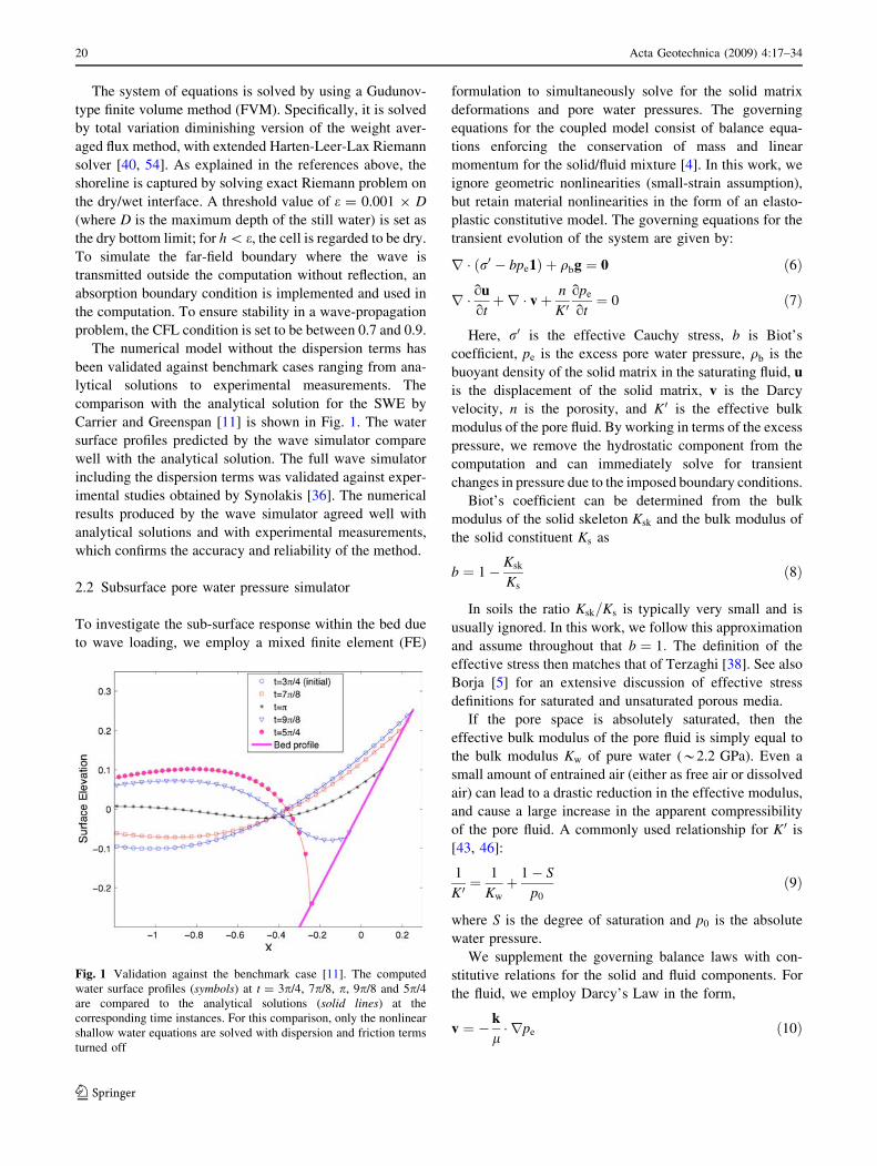
The numerical model without the dispersion terms has

been validated against benchmark cases ranging from ana-

lytical solutions to experimental measurements. The

comparison with the analytical solution for the SWE by

Carrier and Greenspan [11] is shown in Fig. 1. The water

surface profiles predicted by the wave simulator compare

well with the analytical solution. The full wave simulator

including the dispersion terms was validated against exper-

imental studies obtained by Synolakis [36]. The numerical

results produced by the wave simulator agreed well with

analytical solutions and with experimental measurements,

which confirms the accuracy and reliability of the method.

2.2 Subsurface pore water pressure simulator

To investigate the sub-surface response within the bed due

to wave loading, we employ a mixed finite element (FE)

formulation to simultaneously solve for the solid matrix

deformations and pore water pressures. The governing

equations for the coupled model consist of balance equa-

tions enforcing the conservation of mass and linear

momentum for the solid/fluid mixture [4]. In this work, we

ignore geometric nonlinearities (small-strain assumption),

but retain material nonlinearities in the form of an elasto-

plastic constitutive model. The governing equations for the

transient evolution of the system are given by:

r � r0 � bpe1ð Þ þ qbg ¼ 0 ð6Þ

r � ou

otþr � vþ n

K 0ope

ot¼ 0 ð7Þ

Here, r0 is the effective Cauchy stress, b is Biot’s

coefficient, pe is the excess pore water pressure, qb is the

buoyant density of the solid matrix in the saturating fluid, u

is the displacement of the solid matrix, v is the Darcy

velocity, n is the porosity, and K 0 is the effective bulk

modulus of the pore fluid. By working in terms of the excess

pressure, we remove the hydrostatic component from the

computation and can immediately solve for transient

changes in pressure due to the imposed boundary conditions.

Biot’s coefficient can be determined from the bulk

modulus of the solid skeleton Ksk and the bulk modulus of

the solid constituent Ks as

b ¼ 1� Ksk

Ks

ð8Þ

In soils the ratio Ksk=Ks is typically very small and is

usually ignored. In this work, we follow this approximation

and assume throughout that b ¼ 1: The definition of the

effective stress then matches that of Terzaghi [38]. See also

Borja [5] for an extensive discussion of effective stress

definitions for saturated and unsaturated porous media.

If the pore space is absolutely saturated, then the

effective bulk modulus of the pore fluid is simply equal to

the bulk modulus Kw of pure water (*2.2 GPa). Even a

small amount of entrained air (either as free air or dissolved

air) can lead to a drastic reduction in the effective modulus,

and cause a large increase in the apparent compressibility

of the pore fluid. A commonly used relationship for K 0 is

[43, 46]:

1

K 0¼ 1

Kw

þ 1� S

p0

ð9Þ

where S is the degree of saturation and p0 is the absolute

water pressure.

We supplement the governing balance laws with con-

stitutive relations for the solid and fluid components. For

the fluid, we employ Darcy’s Law in the form,

v ¼ � k

l� rpe ð10Þ

Fig. 1 Validation against the benchmark case [11]. The computed

water surface profiles (symbols) at t = 3p/4, 7p/8, p, 9p/8 and 5p/4

are compared to the analytical solutions (solid lines) at the

corresponding time instances. For this comparison, only the nonlinear

shallow water equations are solved with dispersion and friction terms

turned off


123

where k is a tensor of intrinsic permeabilities (with typical

units of m2) and l is the dynamic viscosity of the fluid. An

isotropic medium can be represented with a single scalar

permeability k such that k ¼ k1; where 1 is the second-

order unit tensor. In this work we assume that all perme-

ability fields are isotropic.

An elastoplastic constitutive model for the effective

stress can be written in general incremental form as,

Dr0e ¼ Cep : De; e ¼ 1

2ðruþrtuÞ ð11Þ

where Cep is a non-constant, fourth-order tensor of tangent

moduli relating strain increments ðDeÞ to effective stress

increments ðDr0eÞ: This tensor accounts for the drained

behavior of the soil skeleton. In the elastic regime, we adopt

a linear model for the sand behavior. In this case the tangent

moduli are constant and can be defined by any two elastic

parameters describing the response of the porous skeleton,

e.g., the drained bulk modulus Kd and Poisson ratio m: Note

that this linear-elastic model is a simplified assumption. In

most sands, some degree of pressure-dependence on the

bulk and shear moduli is commonly observed.

In order to define the plastic behavior, we adopt a non-

associative Mohr–Coulomb (MC) model. Under plane-

strain conditions, let the in-plane principal stresses be given

by r01 and r03: The out-of-plane principal stress r02 is

assumed to remain intermediate and has no effect on plastic

yielding. Using the solid mechanics convention, tensile

stresses are positive. Let the mean normal effective stress

and mean shear effective stress be given by,

rm ¼r01 þ r03

2and sm ¼

r01 � r032

ð12Þ

The MC yield surface is implicitly defined as

F ¼ smj j þ rm sinð/Þ � c cosð/Þ ¼ 0 ð13Þ

where / is the friction angle for the sand, and c is the

cohesion. Sands typically display little to no cohesion, and

so c � 0: The plastic potential is similarly defined as,

G ¼ smj j þ rm sinðwÞ � c cosðwÞ ð14Þ

where the friction angle is now replaced with the dilatancy

angle w: Choosing w ¼ / results in an associative model,

while allowing the dilatancy angle to be less than the

friction angle results in a non-associative model. In gen-

eral, w�/ is required to ensure non-negative plastic

dissipation. Non-associative models are typically preferred

for modeling geomaterial behavior, as associative models

tend to overpredict plastic volumetric deformations.

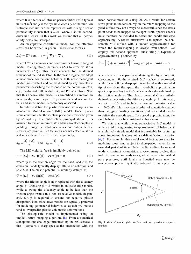
The elastoplastic model is implemented using an

implicit return-mapping algorithm [8]. From a numerical

standpoint, one challenge introduced by the MC surface is

that it contains a sharp apex at the intersection with the

mean normal stress axis (Fig. 2). As a result, for certain

stress paths in the tension region the return mapping to the

yield surface may not always be successful, since the stress

point needs to be mapped to the apex itself. Special checks

must therefore be included to detect and handle this case

appropriately. A robust alternative is to replace the non-

smooth MC surface with a smooth approximation for

which the return-mapping is always well-defined. We

employ this second approach, substituting a hyperbolic

approximation [1] defined by

�F ¼ s2m þ ½ac cosð/Þ�2

h i1=2

þrm sinð/Þ � c cosð/Þ ¼ 0

ð15Þ

where a is a shape parameter defining the hyperbolic fit.

Choosing a ¼ 0; the original MC surface is recovered,

while for a [ 0 the sharp apex is replaced with a rounded

tip. Away from the apex, the hyperbolic approximation

quickly approaches the MC surface, with a slope defined by

the friction angle /: The plastic potential �G is similarly

defined, except using the dilatancy angle w: In this work,

we set a ¼ 0:5; and included a nominal cohesion value

c ¼ 0:05 kPa: This cohesion is orders of magnitude smaller

than the typical loading conditions, and is included merely

to define the smooth apex. To a good approximation, the

sand behavior can be considered cohesionless.

We note that while the non-associative MC model is

widely used in engineering to approximate soil behavior, it

is a relatively simple model that is unsuitable for capturing

some important features of sand-liquefaction behavior

[6, 7]. For example, this model would be inappropriate for

modeling loose sand subject to short-period waves for an

extended period of time. Under cyclic loading, loose sand

tends to contract volumetrically. Over many cycles, this

inelastic contraction leads to a gradual increase in residual

pore pressures, until finally a liquefied state may be

reached—a process typically referred to as cyclic or

τ m

σm

Mohr-Coulomb (a = 0)

Hyperbolic MC (a = 0.5)

c cos(φ)

sin(φ)1

Fig. 2 Mohr–Coulomb yield surface and its hyperbolic approx-

imation


123

residual liquefaction. The MC model cannot capture the

necessary volumetric compaction in order to model this

process. See, for example, Sassa and Sekiguchi [30], Dunn

et al. [15], and Ou et al. [28] for the numerical studies of

this cyclic liquefaction behavior using more sophisticated

elastoplastic models. In the current study, however, the

primary liquefaction mechanism is instantaneous rather

than cyclic. A sudden drawdown of the water level occurs

as the wave retreats from the shoreline, leading to a sudden

change in the vertical hydraulic gradient profile. In regions

where the excess pore water pressure approaches the sud-

denly reduced effective overburden pressure, the sand may

liquefy. In this case, there is no periodic behavior or cyclic

inelastic deformations. For modeling plastic deformation

induced by the sudden change in loading, the non-asso-

ciative MC model was deemed sufficient.

The FE formulation is supplemented with appropriate

boundary conditions in the form of prescribed pressures,

fluxes, displacements, and tractions (described below). In

summary, the key assumptions used in developing the

above model are that (1) the system remains isothermal, (2)

geometric nonlinearities may be ignored, (3) the com-

pressibility of the solid skeleton is much greater than the

intrinsic compressibility of the solid grains, (4) the porosity

and permeability remain constant and are strain-indepen-

dent, and (5) the domain of interest is close to full

saturation.

The numerical implementation is based on the discrete

variational form of the equations, in which the solid dis-

placements and pore pressures are introduced as primitive

variables (u=p form). The spatial discretization is based on

mixed quadrilateral elements with linear interpolation for

both displacements and pressures. In such mixed formula-

tions, the interpolation spaces must be carefully chosen to

avoid spurious pressure oscillations and sub-optimal con-

vergence behavior [10]. For example, a Lagrangian bilinear-

pressure/bilinear-displacement element is typically unstable

and produces poor results. In this work, we employ the

procedure described by White and Borja [45] to stabilize this

otherwise unstable linear/linear combination. The resulting

stabilized formulation has a variety of advantages, particu-

larly in terms of computational efficiency, in comparison to

standard stable elements. The time-integration is based on a

single-step backward-implicit scheme.

The numerical implementation has been validated

against benchmark analytical and experimental solutions

for coupled consolidation problems [45]. Figure 3 presents

one such study, in which the FE result is compared to the

analytical solution for Terzaghi’s 1D consolidation prob-

lem [38]. The problem examines a 1-m thick soil layer atop

a rigid, impermeable base. At t = 0, the saturated soil layer

is suddenly subjected to a uniform strip load of 1 kPa,

while the surface pressure is maintained at atmospheric

conditions. Figure 3 presents the excess pressure profile

with depth at several time instances, illustrating the gradual

dissipation of pressure as drainage proceeds.

3 Validation studies

3.1 Overview of experimental study

To validate the numerical models, the results are compared

with experimental measurements collected from a large-

scale laboratory study of tsunami propagation and sediment

transport over a fine sand beach. The experiments were

conducted at the Tsunami Wave Basin at the Oregon State

University O.H. Hinsdale Wave Research Laboratory in

2007 [48–50]. A 2D flume with dimensions 48.8 m 9

2.16 m wide 9 2.1 m deep was especially built for this

experiment inside the 3D tsunami wave basin.

Natural fine sand from Oregon was used to construct the

mobile bed for this experiment. The sand had a median

diameter D50 = 0.21 mm, and a uniformity coefficient

Cu = D50/D10 = 1.67. The particle fall velocity, specific

gravity, and porosity of a reconstituted laboratory sample

were estimated to be 2.9 cm/s, 2.65, and 0.39, respectively.

The fall velocity was estimated according to the method of

Jimenez and Madsen [17].

In the experiment, numerous sensors were deployed to

measure the water surface elevation, flow velocity, sedi-

ment concentration, pore water pressure, and bed profile,

along with many above water and underwater video

recordings [48–50]. Details about the facilities, instruments,

bed configurations, wave conditions, and experimental

procedures were presented in Young and Xiao [48, 49] and

Young et al. [50].

-1.0

-0.8

-0.6

-0.4

-0.2

0.0

0.0 0.2 0.4 0.6 0.8 1.0

Dep

th (

m)

Pressure (kPa)

FEMExact

5s

20s

50s

100s

200s

Fig. 3 Benchmark comparison of analytical (solid line) and finite

element (dashed line with open circles) solutions to Terzaghi’s 1D

consolidation problem at several time instances


123

In this paper, we will focus our attention to com-

parisons with experimental data obtained near the initial

shoreline for the case of a 60-cm solitary wave propa-

gating over a fine sand beach with a nominal 1:15 slope.

The initial water depth was 1 m. Although numerous

sensors were deployed in the experimental study, we

will only present the measured time-histories from the

wave gauges and pore water pressure sensors at the

initial shoreline, x = 27 m. The locations of the sensors

where comparisons with numerical predictions are

shown in the schematic drawing of the wave flume in

Fig. 4. The waves were generated by a piston wave

maker at x = 0 m and propagated toward the slope on

the right. It should be noted that the region near the

coastline is the area of focus because of its importance

to coastal structure and coastal ecology, and because

that is the region most susceptible to liquefaction

failure.

The setup of the numerical models is shown in Fig. 5.

As explained in the previous section, the wave simula-

tion is carried out using the FVM described in Sect. 2.1,

and the pore water pressure simulation is carried out

using the FE analysis described in Sect. 2.2. As shown

in Fig. 5, the initial bed profile for the 60 cm solitary

waves exhibited a slight S-shape, which is the result of

many previous solitary waves of smaller amplitude. The

grid used for the FE analysis, and the location of the

assumed subsurface water table separating the saturated

and unsaturated portions of the sand bed are also

depicted in Fig. 5. The FVM model simulated the full

cross-shore extent of the flume, from 0 to 41.5 m, to

capture the wave runup and drawdown. The FE model

only simulated the saturated portion of the sand bed, i.e.,

the unsaturated portion above the subsurface water table

was not modeled. The FVM and FE models are not

coupled since the time scale is more than an order of

magnitude different between the surface and subsurface

hydrodynamics for nearly saturated fine sand beach

subject to rapid breaking solitary wave runup and

drawdown.

3.2 Predicted vs. measured wave and pore pressure

time histories

Comparison of the predicted and measured surface water

elevation at WG1 (x = 10 m) and WG12 (x = 27 m) is

shown in Figs. 6 and 7, respectively. Also shown in Fig. 6 is

the theoretical profile according to Munk [22], validating the

accuracy of the wave maker. For the 60 cm solitary wave, a

plunging breaker initiated immediately after x = *22 m at

t * 7.5 s, which impinged on the shallow water near the

shore at x = *24 m. The broken wave formed a turbulent

bore with a height of *20 cm at x = *26 m, which then

climbed onshore. The wave reached its maximum runup at

x = *38.5 m at t = *13 s, followed immediately by

wave drawdown. The drawdown wave reached the position

of the initial shoreline at around t = *15 s, leading to a

hydraulic jump at x = 24 m due to transition from super-

critical to subcritical flow caused by the sudden deceleration

as a result of the collision between the rapidly retreating

water tongue and the relatively still massive body of water.

The drawdown wave continued to travel offshore and

reached WG1 at x = 10 m at t * 20 s. Considering the

complex wave breaking, bore formation and collapse pro-

cesses, the agreement between the numerical predictions

and experimental measurements is satisfactory. It is

important to note that at t [ 20 s, wave–wave interactions

became important, and the flow is complicated by a

hydraulic jump and a large re-circulating flow immediately

seaward of the hydraulic jump. The depth-averaged model

cannot represent these interactions accurately. Therefore,

the agreement after t = 20 s begins to deteriorate. However,

the overall agreement of the numerical predictions and

experimental measurements is relatively good for WG1 and

WG12. Similar good comparisons were also observed at the

14 other locations where different wave gauges and ultra-

sonic sensors were deployed, but they are not shown in this

paper due to space limitations.

The hydrostatic pressure distribution at the bed surface

is applied as a dynamic boundary condition for the FE

analysis of the soil deformation fields and pore pressure

10m 21m 25m 27m23m19m17m15m12m 29m 32m0m 41.5m

Legend: = Wave gauges= Pore pressure sensors

z

x1m

79cm

1:15

PPS8

34cmPPS6

PPS7

PPS5

Still water lineWG1 WG12

Fig. 4 Elevation view of the experimental setup. The triangular area between 12 and 41.5 m is the mobile (sand) bed, which sits on the concrete

bottom of the flume. The circles and squares indicate the locations where the experimental results are compared with numerical predictions


123

distributions. Figure 5 illustrates the geometry and mesh

used for this analysis. The water table was assumed to be

flat and in line with the still waterline, i.e., at z = 0 m. The

assumption of a flat water table seems reasonable in this

case given the idealized experimental setup. A preliminary

analysis of boundary sensitivities indicated that the vadose

zone (the unsaturated portion of beach above the subsur-

face water table) had only minor influence on the pore

pressure distributions on the phreatic zone (the nearly

saturated region below the subsurface water table).

Therefore, for the purposes of this analysis, only the

phreatic zone was modeled. Note, however, that this

implies a fixed phreatic surface which does not move with

the wave-motion. In reality, water table fluctuations are

observed, especially near the intersection of the water table

line with the bed boundary. Given that the inundation

process is very rapid in comparison to the permeability of

the sand, these fluctuations are expected to be quite small

and should not change the results significantly. Further

exploration of this aspect, however, can be found in Niel-

sen [23] and Teo et al. [37].

Constitutive parameters used for the FE analysis are

given in Table 1. These values are consistent with typical

dense fine sand, and were calibrated to provide a good match

with the experimental measurements. The permeability field

unsaturated region (not modeled)

water table

water surface

sand bed

0 m

-1 m

42 m27 m12 mconcrete base

Fig. 5 Schematic of the setup for the numerical model, including the FE mesh configuration used for the subsurface pore water pressure analysis

Fig. 6 Comparison of the theoretical and measured wave elevation

time history at x = 10 m

Fig. 7 Comparison of the predicted and measured wave elevation

time history at x = 27 m

Table 1 Parameter values used in the subsurface finite element

analysis

Permeability k 1.5 9 10-12 m2

Porosity n 0.39

Pore fluid bulk modulus K 0 4 MPa

Drained bulk modulus Kd 85 MPa

Poisson ratio m 0.4

Friction angle / 35�Dilatancy angle w 20�Cohesion c 0.05 kPa

Hyperbolic shape parameter a 0.5


123

was assumed to be isotropic and homogenous. Also, obser-

vations during the wave tank experiments indicated that the

sand had not reached complete saturation despite the many

days of soaking before the 60 cm wave runs. The effective

modulus for the pore fluid was taken to be K 0 ¼ 4 MPa;

corresponding to 97% saturation. We hypothesize that the

presence of residual air accounts for the apparent increase in

compressibility of the pore fluid in comparison to that of

pure water.

The lower boundary representing the concrete base was

considered a zero-flux, zero-displacement boundary. The

right boundary representing the concrete wall was also

considered a zero-flux, zero-displacement boundary. The

upper boundary is broken into two sections, one repre-

senting the exposed bed surface, and one representing the

flat water table line. The pressure at the bed surface was

assigned based on the excess hydrostatic pressure caused

by the wave motion, �pwave: The excess pressure on the

water table surface was set to 0 (gauge atmospheric). By

definition, the traction at these boundaries is given by

t ¼ r � n ¼ r0 � n� pen ð16Þ

where n is the unit normal to the surface. Since the sand

bed boundary is in contact with water only, the effective

stress should be 0 there. To enforce this condition, it is

therefore necessary to apply a traction such that

twave ¼ ��pwaven ð17Þ

On the water table boundary, the excess pressure is zero,

but the effective stress is not zero as a result of two

components: the weight of the unsaturated soil above the

water table, and the weight of the passing wave. For the

wave component we can again use Eq. (17). This implies

that the traction given by Eq. (17) should be applied at both

the bed surface boundary and the water table boundary,

though the resulting effective stress states are quite

different.

Figure 8 presents the predicted and measured time his-

tories of the evolution of the change in pore pressure from

the initial hydrostatic state at the four pore pressure sensors

(PPS5–8) deployed at the initial shoreline (x = 27 m). The

location of the pore pressure sensors is shown in Fig. 4.

They are spaced 0.15 m apart vertically. PPS8 is on the

top, and it is located 0.16 m from the bed surface. The pore

pressure distribution at PPS8 corresponded well with the

variations in water surface elevations shown in Fig. 7,

confirming the validity of the hydrostatic pressure

assumption. The simulation was performed using both a

linear-elastic model and the elastoplastic model described

earlier. Both models produced essentially identical results.

Plastic deformations therefore do not play a significant role

in this case due to the rapid loading and unloading of the

0

0.5

1

0 5 10 15 20

Pre

ssur

e (k

Pa)

Time (s)

PPS 5

z = -0.66 m

0

0.5

1

Pre

ssur

e (k

Pa)

PPS 6

z = -0.51 m

0

0.5

1

Pre

ssur

e (k

Pa)

PPS 7

z = -0.36 m

0

0.5

1

Pre

ssur

e (k

Pa)

PPS 8z = -0.21 m

MeasuredElastic ModelPlastic Model

Fig. 8 Comparison of the predicted and measured pore water pressure at x = 27 m. The z-values indicated in the graphs are measured from the

bed surface at x = 27 m


123

model-scale experiment. The sudden rise in pore pressure

at PPS5–7 around the 4 s is attributed to the compression

of the solid skeleton due to the arrival of the wave at the

bed surface. A pure diffusion model does not capture this

sudden rise—a key advantage of the coupled solid/fluid

formulation. The first and second peaks observed in PPS5–

8 corresponded to the passing of the water column asso-

ciated with wave runup and drawdown, respectively. In

both the experimental measurements and numerical pre-

dictions, the diffusive behavior of the pressure waves can

be discerned by the increases in time lags in peak arrivals,

decreases in peak magnitude, and increases in blurring of

the peaks and troughs. As shown in Fig. 8, the agreement

between numerical predictions and experimental mea-

surements is quite good for t \ 13 s. The agreement begins

to deteriorate for t [ 13 s due to small errors in the sim-

ulated wave profile caused by wave–wave interactions,

hydraulic jump, and large re-circulating flow that occurred

at the end of the drawdown. It is important that to note that

since the pore pressure is governed primarily by diffusion,

small changes in the boundary condition (e.g., bed surface

pressure distribution) can lead to much larger change in the

pore pressure distributions. Nevertheless, considering the

complexity of the experiment, and the spatial variation of

the porosity, saturation, and grain size caused by repeated

wave actions, the overall agreement between the numerical

predictions and experimental measurements is satisfactory.

4 Results

4.1 Overview of model setup

Numerical case studies are presented for a full-scale prob-

lem: a solitary wave with an initial height 10 m propagating

over an initial water depth of 20 m. The slope of the fine

sand beach is selected to be 1:15 and 1:5 to represent a mild

slope and a steep slope beach, respectively. The depth of the

sand layer to impervious bedrock is assumed to be 20 m.

The properties of the sand are the same as given in Table 1.

The top and bottom boundary conditions are the same as

those used in Sect. 3. The left (landward) and right (sea-

ward) boundaries are approximated as zero-flux, zero

horizontal displacement boundaries. Although some flux is

expected across the left and right boundaries as the wave

passes, the vertical flux is assumed to dominate. This

approximation is used because there is no a priori estimate

of the pressure or flux profile with depth. Hence, the left and

right boundaries are purposely placed far enough away such

that the error introduced by the zero-flux boundary condi-

tions has negligible impact in the region of interest, the

near-shore region. The model setup for the 1:5 case is

shown in Fig. 9. The water table profile is again assumed to

be flat and stationary, though we note that for most natural

beaches the water table shows some vertical variation. The

wave profiles during the runup and drawdown, as well as the

bed responses for the two different slopes are studied and

compared.

The objectives of the case studies are to assess and

compare the time, extent, and location of zones with a high

potential for liquefaction. There are a variety of criteria we

could use to assess liquefaction potential. In this work, we

use one based on the mean normal effective stress rm:

When the normal stress is negative (compression), the sand

has some shear capacity and is assumed to be in an un-

liquefied state. Pore pressure increases, however, can cause

the mean normal effective stress to exceed the limited

tensile strength of the sand. In the process, the local shear

capacity decreases until no residual strength is left. The

stress point then lies at the apex of the MC yield surface.

Since sands are typically cohesionless, the liquefaction

threshold used in this work is simply rm ¼ 0: We note that

in defining the smoothed MC model, we have added a

nominal cohesion value (0.05 kPa) that allows the mean

normal stress to rise slightly above 0, but this slight

cohesion is ignored in assessing liquefaction potential.

water surface

bed surface

watertable

unsaturated zone(not modeled)

impermeable, rigid bed

51

0 m

-20 m

-20 m 0 m

100 m

-40 m

-20 m

Fig. 9 Model setup for the numerical simulation of a 10-m solitary wave running onto a 1:5 bed slope


123

Another issue that must be addressed is the time-varia-

tion of the liquefied zone. As the wave evolves, the mean

normal effective stress at a point in the sand may increase

to 0, but then later drop below the liquefaction threshold. In

this work we make no attempt to model post-liquefaction

or solidification behavior, during which the sand has an

entirely different constitutive behavior. In assessing liq-

uefaction potential, our primary concern is whether a point

in the soil ever liquefies, and base the liquefaction criterion

on the cumulative maximum mean normal stress a point

encounters over the course of the wave loading.

4.2 Wave propagation—1:15 slope

The runup and drawdown wave profiles of a 10-m solitary

wave over a 1:15 sandy slope is shown in Fig. 10. The wave

is centered at x = 340 m at t = 0 s. The wave profiles

during the runup and drawdown are shown in the left and the

right plots, respectively. The time stamps corresponding to

the profiles are indicated in the legend, with units of seconds.

The wave shoaling on the slope is discernable by the fact that

the wave height at t = 12.79 s is slightly greater than the

initial height of 10 m. The wave breaking can be observed

from the decrease in wave height between t = 12.79 and

t = 19.18 s. The maximum runup occurred at t = 49.4 s

with the maximum horizontal excursion at x = -233 m.

After which, drawdown begins. The drawdown caused the

water level to drop *4 m below the still waterline, which

exposed a 50-m wide by 4 m deep area immediately below

the initial shoreline. During the drawdown, a hydraulic jump

formed at x = 45 m, which lasted for *30 s.

The time-histories of the wave surface profile at x = 0

(shoreline), 25, and 40 m are shown in Fig. 11. Notice that

the wave broke more than 50 m offshore, and hence the

maximum wave height at x = 40 m is only *7.5 m. The

wave height continues to decrease as it propagates onshore

due to energy dissipation via friction. At the shoreline

(x = 0 m), the maximum wave height is only slightly higher

than 5 m. At x = 40 m, the rate of bed surface pressure drop

is approximately 70 kPa in 25 s, which can be considered as

sudden since the drainage time of the pore pressure for 20 m

of nearly saturated fine sand is estimated to be approximately

1,500 s based on the soil properties assumed in Table 1.

4.3 Pore pressure responses—1:15 slope

The left plots on Fig. 12 presents the time-histories of the

predicted excess pore pressures for the 1:15 bed at

x = 40 m during the wave runup and drawdown processes.

The results are sampled at six points at increasing depths,

in 30 cm increments. The cross-shore location of the

sampled section, x = 40 m, is chosen because it is in close

Fig. 10 Selected wave profiles for a 10-m solitary wave propagating onto a 1:15 slope. Left wave profiles during runup. Right wave profiles

during drawdown. The maximum runup occurred at t = 49.4 s with the maximum horizontal excursion at x = -233 m. The time (t) stamps are

in units of seconds

Fig. 11 Time series of wave elevation at three different locations:

40 m offshore, 25 m offshore, and at the shoreline, recorded from the

numerical simulation of a 10-m wave running onto a 1:15 slope bed


123

proximity to the hydraulic jump that formed during the

wave drawdown. At this point, the maximum drop in water

level is observed, and this cross-section is thus considered

critical in terms of liquefaction potential.

The simulation was again performed with two material

models, a linear-elastic model and the elastoplastic model.

In this case, significant differences are observed in the two

models. The time-history of the excess pore pressure at the

bed surface, z = 0 m, is equivalent to the transient varia-

tions in water surface elevation. During the runup phase,

the soil is subject to compression due to increase in bed

surface traction caused by the passing of the wave, which

-40

-20

0

20

0 20 40 60 80 100 120

Pre

ssur

e (k

Pa)

Time (s)

z = -1.50 m, elasticplastic

-40

-20

0

20

Pre

ssur

e (k

Pa)


-40

-20

0

20

Pre

ssur

e (k

Pa)


-40

-20

0

20

Pre

ssur

e (k

Pa)


-50

-25

0

25

50

Pre

ssur

e (k

Pa)


-50

0

50

100

Pre

ssur

e (k

Pa)

1:15 Slope, x = 40m

z = 0.00 m, elasticplastic

-40

-20

0

20

0 20 40 60 80 100 120

Pre

ssur

e (k

Pa)

Time (s)


-40

-20

0

20

Pre

ssur

e (k

Pa)


-40

-20

0

20

Pre

ssur

e (k

Pa)


-40

-20

0

20

Pre

ssur

e (k

Pa)


-50

-25

0

25

50

Pre

ssur

e (k

Pa)


-50

0

50

100

Pre

ssur

e (k

Pa)

1:5 Slope, x = 25m

z = 0.00 m, elasticplastic

Fig. 12 Time histories of excess pore pressure for the 1:15 slope at x = 40 m (left) and the 1:5 slope at x = 25 m (right). The z locations are

measured from the bed surface at the respective locations


123

Fig. 13 Snapshots of the wave motion and contours of the cumulative maximum mean normal stress (rm) in the 1:15 slope at several time

instants. The high liquefaction potential zone (rm = 0) corresponds to the black region


123

leads to buildup of excess pore pressure, particularly in the

top soil layer. For soil at or deeper than 60 cm beneath the

surface, an instantaneous rise in pore pressures at

t = *18 s can be observed, and it is a result of the

immediate compression of the solid skeleton due to the

sudden increase in overburden stress caused by arrival of

the wave. During the drawdown phase, the soil is subject to

decompression. The bed surface pressure drops to the

atmospheric pressure as the surface water level drops to 0.

However, the excess pore pressure beneath the bed surface

cannot dissipate as fast, which leads to negative (upward)

vertical pore pressure gradients that may cause liquefaction

failure of the soil near the bed surface.

Both the elastic and elastoplastic models are able to

capture the classic diffusive nature of the excess pore water

pressure, which is evident via the increases in time lag in

the arrival of the peaks, the decreases in the magnitude of

the peaks, and the blurring of the peaks. The pore pressure

responses predicted by the two models are essentially

identical during the loading phase. However, significant

differences can be observed during the unloading phase;

the elastoplastic model predicts significantly larger nega-

tive pressures, with much less dissipation with depth than

the elastic model. The predominant deformation mecha-

nism in these simulations is volumetric, rather than

deviatoric, and hence the loading and unloading is close to

the hydrostatic axis. When the soil is subject to compres-

sion during the runup, the elastic and MC models should

produce identical results. On the other hand, when the soil

is subject to decompression during the drawdown, the

elastic and MC models should produce different results.

The elastic model can maintain large tensile stresses, and

therefore accommodate high local pressures (and thus

higher local pressure gradients). The MC model deforms

plastically under large decompression, and so the pressure

difference induced by the wave loading must be accom-

modated over a much larger depth. As a result, the

hydraulic gradient for the elastic model is higher, but

penetrates to a shallower depth, than the MC model.

To assess the liquefaction potential, we use the cumu-

lative maximum mean normal effective stress criterion

described earlier. If the pore pressure conditions are such

that rm ever equals 0, the sand is assumed to have lique-

fied. Figure 13 presents a spatial picture of the growth of

the liquefaction zone based on the elastoplastic material

model. The maximum depth of the liquefaction zone is

predicted to be 2.8 m.

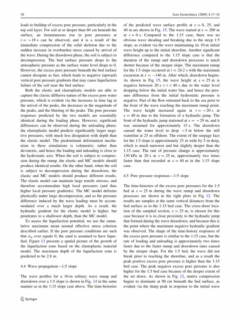
4.4 Wave propagation—1:5 slope

The wave profiles for a 10-m solitary wave runup and

drawdown over a 1:5 slope is shown in Fig. 14 in the same

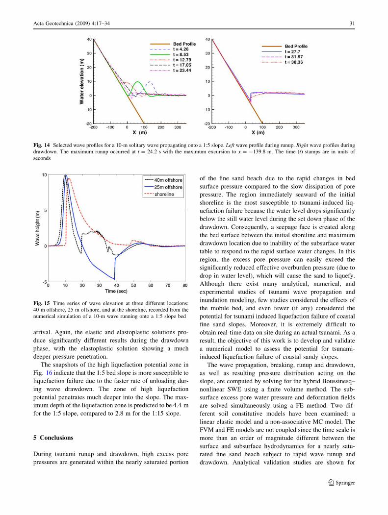
manner as in the 1:15 slope case above. The time-histories

of the predicted wave surface profile at x = 0, 25, and

40 m are shown in Fig. 15. The wave started at x = 200 m

at t = 0 s. Compared to the 1:15 case, there was no

obvious wave shoaling and breaking due to the steep 1:5

slope, as evident via the wave maintaining its 10-m initial

wave height up to the initial shoreline. Another significant

difference compared to the 1:15 slope case is that the

duration of the runup and drawdown processes is much

shorter because of the steeper slope. The maximum runup

for the 1:5 slope occurred at t = 24.2 s with the maximum

excursion at x = -140 m. After which, drawdown begins.

As shown in Fig. 15, the wave height at x = 25 m is

negative between 20 s \ t \ 40 s due to the water level

dropping below the initial water line, and hence the pres-

sure difference from the initial hydrostatic pressure is

negative. Part of the flow retreated back to the sea prior to

the front of the wave reaching the maximum runup point.

The wave height increased again at t = *20 s at

x = 40 m due to the formation of a hydraulic jump. The

front of the hydraulic jump stationed at x = *29 m, and it

was sustained for approximately 15 s. The drawdown

caused the water level to drop *5 m below the still

waterline at 25 m offshore. The extent of the seepage face

for the 1:5 slope is approximately 25 m wide by 5 m deep,

which is much narrower and but slightly deeper than the

1:15 case. The rate of pressure change is approximately

130 kPa in 20 s at x = 25 m, approximately two times

faster than that recorded at x = 40 m in the 1:15 slope

case.

4.5 Pore pressure responses—1:5 slope

The time-histories of the excess pore pressures for the 1:5

bed at x = 25 m during the wave runup and drawdown

processes are shown in the right plots in Fig. 12. The

results are samples at the same vertical distances from the

bed surface as in the 1:15 bed case. The cross-shore loca-

tion of the sampled section, x = 25 m, is chosen for this

case because it is in close proximity to the hydraulic jump

that formed during the wave drawdown, and because this is

the point where the maximum negative hydraulic gradient

was observed. The shape of the time-history responses of

the excess pore pressure is similar to the 1:15 case, but the

rate of loading and unloading is approximately two times

faster due to the faster runup and drawdown rates caused

by the steeper slope. For the 1:5 bed, the wave did not

break prior to reaching the shoreline, and as a result the

peak positive excess pore pressure is higher than the 1:15

bed case. The peak negative excess pore pressure is also

higher for the 1:5 bed case because of the deeper extent of

the set down. As shown in Fig. 12, matrix compression

begins to dominate at 90 cm beneath the bed surface, as

evident via the sharp peak in response to the initial wave


123

arrival. Again, the elastic and elastoplastic solutions pro-

duce significantly different results during the drawdown

phase, with the elastoplastic solution showing a much

deeper pressure penetration.

The snapshots of the high liquefaction potential zone in

Fig. 16 indicate that the 1:5 bed slope is more susceptible to

liquefaction failure due to the faster rate of unloading dur-

ing wave drawdown. The zone of high liquefaction

potential penetrates much deeper into the slope. The max-

imum depth of the liquefaction zone is predicted to be 4.4 m

for the 1:5 slope, compared to 2.8 m for the 1:15 slope.

5 Conclusions

During tsunami runup and drawdown, high excess pore

pressures are generated within the nearly saturated portion

of the fine sand beach due to the rapid changes in bed

surface pressure compared to the slow dissipation of pore

pressure. The region immediately seaward of the initial

shoreline is the most susceptible to tsunami-induced liq-

uefaction failure because the water level drops significantly

below the still water level during the set down phase of the

drawdown. Consequently, a seepage face is created along

the bed surface between the initial shoreline and maximum

drawdown location due to inability of the subsurface water

table to respond to the rapid surface water changes. In this

region, the excess pore pressure can easily exceed the

significantly reduced effective overburden pressure (due to

drop in water level), which will cause the sand to liquefy.

Although there exist many analytical, numerical, and

experimental studies of tsunami wave propagation and

inundation modeling, few studies considered the effects of

the mobile bed, and even fewer (if any) considered the

potential for tsunami induced liquefaction failure of coastal

fine sand slopes. Moreover, it is extremely difficult to

obtain real-time data on site during an actual tsunami. As a

result, the objective of this work is to develop and validate

a numerical model to assess the potential for tsunami-

induced liquefaction failure of coastal sandy slopes.

The wave propagation, breaking, runup and drawdown,

as well as resulting pressure distribution acting on the

slope, are computed by solving for the hybrid Boussinesq–

nonlinear SWE using a finite volume method. The sub-

surface excess pore water pressure and deformation fields

are solved simultaneously using a FE method. Two dif-

ferent soil constitutive models have been examined: a

linear elastic model and a non-associative MC model. The

FVM and FE models are not coupled since the time scale is

more than an order of magnitude different between the

surface and subsurface hydrodynamics for a nearly satu-

rated fine sand beach subject to rapid wave runup and

drawdown. Analytical validation studies are shown for

Fig. 14 Selected wave profiles for a 10-m solitary wave propagating onto a 1:5 slope. Left wave profile during runup. Right wave profiles during

drawdown. The maximum runup occurred at t = 24.2 s with the maximum excursion to x = -139.8 m. The time (t) stamps are in units of

seconds

Fig. 15 Time series of wave elevation at three different locations:

40 m offshore, 25 m offshore, and at the shoreline, recorded from the

numerical simulation of a 10-m wave running onto a 1:5 slope bed


123

Fig. 16 Snapshots of the wave motion and contours of the cumulative maximum mean normal stress in the 1:5 slope at several time instants. The

high liquefaction potential zone corresponds to the black region


123

both the wave simulation model and the soil pore water

pressure model. Experimental validation studies are also

shown using results from a large-scale laboratory study of

breaking solitary wave runup and drawdown over a fine

sand beach. Good comparisons were observed from both

the analytical and experimental validation studies.

Numerical case studies are shown for a full-scale sim-

ulation of a 10-m solitary wave over a 1:15 and 1:5 sloped

fine sand beach. The results show that the soil near the bed

surface is subject to liquefaction failure, with the deepest

liquefaction zone near the seepage face. The depth of the

seepage face increases and the width of the seepage face

decreases with increasing bed slope. The rate of loading

and unloading also increases with increasing bed slope.

Consequently, the hydraulic gradient increases with

increasing bed slope. As a result, the case with the steeper

slope is more susceptible to liquefaction failure. The results

show that the cross-shore extent of the zone of high liq-

uefaction potential is narrower for the 1:5 bed due to the

smaller width of the seepage face, but the depth is

approximately the same between the two different slopes.

The analysis also suggests that the results are highly

influenced by the soil permeability and relative compress-

ibility between the pore fluid and solid skeleton, and that a

coupled solid/fluid formulation is needed for the soil sol-

ver. The results suggest that the influence of nonlinear

material behavior is negligible for the model-scale labo-

ratory simulation due to the rapid loading and unloading.

However, for the full-scale case studies with 10-m solitary

waves, significant differences can be observed between the

elastic and elastoplastic models during the drawdown

phase. The MC elastoplastic model predicted significantly

larger negative pressures, with much less dissipation with

depth than the elastic model because the soil behaves

plastically under decompression. Consequently, the

hydraulic gradient for the elastic model is higher, but

penetrates to a shallower depth, than the MC model.

Nevertheless, the current MC model is relatively simple,

and cannot capture important features such as increase in

residual pore pressure due to volumetric compression.

Therefore, additional work is needed to investigate the

influence of nonlinear material behavior and material

instability. Further work is also necessary to determine the

effect of wave shape, wave–wave interaction, bathymetry,

and soil properties on the bed responses.

Acknowledgments The authors would like to acknowledge funding

by the National Science Foundation through the NSF George E.

Brown, Jr Network for Earthquake Engineering Simulation (grant no.

0530759) and through the NSF CMMI grant no. 0653772. The first

author would also like to acknowledge the financial support through

the UPS visiting professor program at Stanford, and the second author

would like to acknowledge the support through the NSF Graduate

Research Fellowship Program.

References

1. Abbo AJ, Sloan SW (1995) A smooth hyperbolic approximation

to the Mohr-Coulomb yield criterion. Comput Struct 54(3):427–

441

2. Bennett RH (1978) Pore-water pressure measurements: Missis-

sippi Delta submarine sediments. Mar Geotechnol 2:177–189

3. Bennett RH, Faris JR (1979) Ambient and dynamic pore pres-

sures in fine-grained submarine sediments: Mississippi. Appl

Ocean Res 1(3):115–123. doi:10.1016/0141-1187(79)90011-7

4. Biot MA (1941) General theory of three-dimensional consolida-

tion. J Appl Phys 12(2):155–164

5. Borja RI (2006) On the mechanical energy and effective stress in

saturated and unsaturated porous continua. Int J Solids Struct

43(6):1764–1786

6. Borja RI (2006) Conditions for instabilities in collapsible solids

including volume implosion and compaction banding. Acta

Geotech 1:107–122. doi:10.1007/s11440-006-0012-x

7. Borja RI (2006) Condition for liquefaction instability in fluid-

saturated granular soils. Acta Geotech 1:211–224. doi:10.1007/

s11440-006-0017-5

8. Borja RI, Sama KM, Sanz PF (2003) On the numerical integra-

tion of three-invariant elastoplastic constitutive models. Comp

Methods Appl Mech Engrg 192:1227–1258

9. Borthwick AGL, Ford M, Weston BP, Taylor PH, Stansby PK

(2006) Proceedings of the Institution of Civil Engineers. J Marit

Eng 159(MA3):97–105. doi:10.1680/maen.2006.159.3.97

10. Brezzi F (1990) A discourse on the stability conditions for mixed

finite element formulations. Comput Methods Appl Mech Eng

82:1–3, 27–57

11. Carrier F, Greenspan HP (1958) Water waves of finite amplitude

on a sloping beach. J Fluid Mech 4:97–109. doi:10.1017/

S0022112058000331

12. Chowdhury B, Dasari GR, Nogami T (2006) Laboratory study of

liquefaction due to wave–seabed interaction. J Geotech Geoen-

viron Eng 132(7):842–851. doi:10.1061/(ASCE)1090-0241

(2006)132:7(842)

13. De Groot MB, Kudella M, Meijers P, Oumeraci H (2006) Lique-

faction phenomena underneath marine gravity structures subjected

to wave loads. J Waterw Port Coast Ocean Eng 132(4):325–335.

doi:10.1061/(ASCE)0733-950X(2006)132:4(325)

14. Demars KR, Vanover EA (1985) Measurements of wave-induced

pressures and stresses in a sand bed. Mar Geotechnol 6(1):29–59

15. Dunn SL, Vun PL, Chan AHC, Damgaard JS (2006) Numerical

modeling of wave-induced liquefaction around pipelines. J

Waterw Port Coast Ocean Eng 132(4):276–288. doi:10.1061/

(ASCE)0733-950X(2006)132:4(276)

16. Jeng DS (2003) Wave-induced sea floor dynamics. Appl Mech

Rev 56(4):407–429. doi:10.1115/1.1577359

17. Jimenez JA, Madsen OS (2003) A simple formula to estimate

settling velocity of natural sediments. J Waterw Port Coast Ocean

Eng 129(2):70–78. doi:10.1061/(ASCE)0733-950X(2003)129:

2(70)

18. Kim DH, Cho YS, Kim WG (2004) Weighted averaged flux-type

scheme for shallow water equations with fractional step method. J

Eng Mech 130(2):152–160. doi:10.1061/(ASCE)0733-9399

(2004)130:2(152)

19. Kudella M, Oumeraci H, de Groot MB, Meijers P (2006)

Large-scale experiments on pore pressure generation under-

neath a Caisson Breakwater. J Waterw Port Coast Ocean

Eng 132(4):310–324. doi:10.1061/(ASCE)0733-950X(2006)132:4

(310)

20. Maeno YH, Hasegawa T (1987) In-situ measurements of wave-

induced pore pressure for predicting properties of seabed

deposits. Coast Eng Japan 30(1):99–115


123

http://dx.doi.org/10.1016/0141-1187(79)90011-7

http://dx.doi.org/10.1007/s11440-006-0012-x

http://dx.doi.org/10.1007/s11440-006-0017-5

http://dx.doi.org/10.1007/s11440-006-0017-5

http://dx.doi.org/10.1680/maen.2006.159.3.97

http://dx.doi.org/10.1017/S0022112058000331

http://dx.doi.org/10.1017/S0022112058000331

http://dx.doi.org/10.1061/(ASCE)1090-0241(2006)132:7(842)


http://dx.doi.org/10.1061/(ASCE)0733-950X(2006)132:4(325)



http://dx.doi.org/10.1115/1.1577359







21. Madsen PA, Murray R, Sørensen OR (1991) A new form of the

Boussinesq equations with improved linear dispersion character-

istics. Part I. Coast Eng 15(4):371–388. doi:10.1016/0378-3839

(91)90017-B

22. Munk W (1949) The solitary wave theory and its application to

surf problems. Ann NY Acad Sci 51:376–423. doi:10.1111/

j.1749-6632.1949.tb27281.x

23. Nielsen P (1990) Tidal dynamics of the water table in beaches.

Water Resour Res 26(9):2127–2134

24. Okusa S (1985) Measurements of wave-induced pore pressure in

submarine sediments under various marine conditions. Mar

Geotechnol 6(2):119–144

25. Okusa S, Uchida A (1980) Pore-water pressure change in sub-

marine sediments due to waves. Mar Geotechnol 4(2):145–161

26. Okusa S, Nakamura T, Fukue M (1983) Measurements of wave-

induced pore pressure and coefficients of permeability of sub-

marine sediments during reversing flow. In: Denness B (ed)

Seabed mechanics. Graham and Trotman Ltd, London, pp 113–

122

27. Onate E, Celigueta MA, Idelsohn SR (2006) Modeling bed ero-

sion in free surface flows by the particle finite element method.

Acta Geotech 1:237–252. doi:10.1007/s11440-006-0019-3

28. Ou J, Jeng DS, Chan AHC (2008) Three-dimensional poro-el-

astoplastic model for wave-induced pore pressure in a porous

seabed around breakwater heads. In: Papadrakakis M, Topping

BHV (eds) Proceedings of the sixth international conference on

engineering computational technology, Paper 1, Stirlingshire

29. Phillips R, Sekiguchi H (1992) Generation of water wave trains in

drum centrifuge. Proc Int Symp Technol Ocean Eng 1:29–34

30. Sassa S, Sekiguchi H (1999) Wave-induced liquefaction of beds

of sands in a centrifuge. Geotechnique 49(5):621–638

31. Schaffer HA, Madsen PA, Deigaard R (1993) A Boussinesq

model for waves breaking in shallow water. Coastal Eng

20(3/4):185–202

32. Sekiguchi H, Phillips R (1991) Generation of water waves in a

drum centrifuge. In: Proceedings of international conference on

centrifuge, Yokohama, pp 343–350

33. Sleath JFA (1970) Wave-induced pressures in beds of sand.

J Hydraul Div 96(2):367–378

34. Sumer BM, Truelsen C, Fredsøe J (2006) Liquefaction around

pipelines under waves. J Waterw Port Coast Ocean Eng 132(4):

266–275. doi:10.1061/(ASCE)0733-950X(2006)132:4(266)

35. Sumer BM, Ansal AK, Cetin KO, Damgaard J, Gunbak AR,

Hansen NEO, Sawicki A, Synolakis CE, Yalciner AC, Yuksel Y,

Zen K (2007) Earthquake-induced liquefaction around marine

structures. J Waterw Port Coast Ocean Eng 133(1):55–82. doi:

10.1061/(ASCE)0733-950X(2007)133:1(55)

36. Synolakis CE (1987) The runup of solitary waves. J Fluid Mech

185:523–545. doi:10.1017/S002211208700329X

37. Teo HT, Jeng DS, Seymour BR, Barry DA, Li L (2003) A new

analytical solution for water table fluctuations in coastal aquifers

with sloping beaches. Adv Water Resour 26:1239–1247. doi:

10.1016/j.advwatres.2003.08.004

38. Terzaghi K (1943) Theoretical soil mechanics. Wiley, New York

39. Tonkin S, Yeh H, Kato F, Sato S (2003) Tsunami scour

around a cylinder. J Fluid Mech 496:165–192. doi:10.1017/

S0022112003006402

40. Toro EF (2000) Shock-capturing methods for free-surface shal-

low flows. Wiley, New York

41. Tsui YT, Helfrich SC (1983) Wave-induced pore pressures in

submerged sand layer. J Geotech Eng Div ASCE 109(4):603–618

42. Tzang SY (1992) Water wave-induced soil fluidization in a

cohesionless fine-grained seabed. PhD Dissertation, University of

California, Berkeley

43. Verruijt A (1969) Elastic storage of aquifers. In: Dewiest RJM

(ed) Flow through porous media. Academic, New York

44. Wei Y, Mao XZ, Cheung KF (2006) Well-balanced finite-volume

model for long wave runup. J Waterw Port Coast Ocean Eng 132(2):

114–124. doi:10.1061/(ASCE)0733-950X(2006)132:2(114)

45. White J, Borja R (2008) Stabilized low-order finite elements for

coupled solid-deformation/fluid-diffusion and their application to

fault zone transients. Comput Methods Appl Mech Eng 197:49–

50, 4353–4366. doi:10.1016/j.cma.2008.05.01

46. Yamamoto T, Koning HL, Sellmeijer H, van Hijum E (1978) On

the response of a poro-elastic bed to water waves. J Fluid Mech

87(1):193–206. doi:10.1017/S0022112078003006

47. Yeh H, Kato F, Sato S (2001) Tsunami scour mechanisms around

a cylinder. In: Hebenstreit GT (ed) Tsunami research at the end of

a critical decade. Kluwer Academic Publishers, Dordrecht, pp

33–46

48. Young YL, Xiao H (2008) Erosion and deposition processes due

to solitary waves over a movable bed. Technical Report 0803,

Department of Civil and Environmental Engineering, Princeton

University, Princeton

49. Young YL, Xiao H (2008) Enhanced sediment transport due to

wave–soil interactions. In: Proceedings of 2008 NSF engineering

research and innovation conference, Knoxville, 8–10 January

2008

50. Young YL, Xiao H, Maddux T. Runup and drawdown of

breaking solitary waves over a fine sand beach. Part I: experi-

mental modeling. Mar Geol (under review)

51. Zen K, Yamazaki H (1990) Mechanism of wave-induced lique-

faction and densification in seabed. Soil Found 30(4):90–104

52. Zen K, Yamazaki H (1991) Field observation and analysis of

wave-induced liquefaction in seabed. Soil Found 31(4):161–179

53. Zhang JE (1996) Run-up of ocean waves on beaches. California

Institute of Technology, Pasadena

54. Zoppou C, Roberts S (2000) Numerical solution of the two-

dimensional unsteady dam break. Appl Math Model 24:457–475.

doi:10.1016/S0307-904X(99)00056-6


123

http://dx.doi.org/10.1016/0378-3839(91)90017-B

http://dx.doi.org/10.1016/0378-3839(91)90017-B

http://dx.doi.org/10.1111/j.1749-6632.1949.tb27281.x

http://dx.doi.org/10.1111/j.1749-6632.1949.tb27281.x

http://dx.doi.org/10.1007/s11440-006-0019-3



http://dx.doi.org/10.1017/S002211208700329X

http://dx.doi.org/10.1016/j.advwatres.2003.08.004

http://dx.doi.org/10.1017/S0022112003006402

http://dx.doi.org/10.1017/S0022112003006402


http://dx.doi.org/10.1016/j.cma.2008.05.01

http://dx.doi.org/10.1017/S0022112078003006

http://dx.doi.org/10.1016/S0307-904X(99)00056-6

liquefaction potential of coastal slopes induced by ...web.stanford.edu/~borja/pub/ag2009(1).pdf ·...

Documents