Liquidity Risk inSequential Trading Networks∗

Shachar Kariv† Maciej H. Kotowski‡ C. Matthew Leister§

October 9, 2017

Abstract

This paper studies a model of intermediated exchange with liquidity-constrainedtraders. Intermediaries are embedded in a trading network and their financial capac-ities are private information. We characterize our model’s monotone, pure-strategyequilibrium. Agents earn positive intermediation rents in equilibrium. An experimen-tal investigation supports the model’s baseline predictions concerning agents’ strate-gies, price dynamics, and the division of surplus. While private financial constraintsinject uncertainty into the trading environment, our experiment suggests they are alsoa behavioral speed-bump, preventing traders from experiencing excessive losses due tooverbidding.

Keywords: Experiment, economic networks, intermediation, liquidity, auctions, budgetconstraintsJEL: L14, C91, D85, D44, G10

∗We thank Douglas Gale for detailed comments and suggestions. We are also grateful to Larry Blume,Gary Charness, Syngjoo Choi, Andrea Galeotti, Edoardo Gallo, Sanjeev Goyal, Tom Palfrey, Brian Rogers,and Bill Zame for helpful discussions and comments. The paper has also benefited from suggestions by theparticipants of seminars at several universities. This research was supported by the UC Berkeley Experimen-tal Social Science Laboratory (Xlab), and the experiments were funded by the Multidisciplinary UniversityResearch Initiatives (MURI) Program—Multi-Layers and Multi-Resolution Networks of Interacting Agentsin Adversarial Environments.

†Department of Economics, University of California, Berkeley, 530 Evans Hall #3880, Berkeley, CA 94720,United States. E-mail: <kariv@berkeley.edu>

‡John F. Kennedy School of Government, Harvard University, 79 JFK Street, Cambridge MA 02138,United States. E-mail: <maciej_kotowski@hks.harvard.edu>

§Department of Economics, Monash University, 900 Dandenong Road, Caulfield East VIC 3145, Australia.E-mail: <matthew.leister@monash.edu>

1

1 IntroductionIn many decentralized markets, intermediary traders link producers and consumers. Twokey variables determine the effectiveness of market intermediaries. First, a trader needs tohave adequate financial resources—either in the form of cash on hand or credit—to pay forthe goods that he wishes to trade. And second, each intermediary depends on his network ofpotential counter-parties to source goods and to find buyers. The interaction between thesevariables raises several open questions:

1. How do intermediary traders account for others’ (possibly) limited financial capacity?

2. What price dynamics might we observe as goods are bought and resold in the market?

3. What are the distributional consequences of the economy’s network structure? Aresome traders systematically advantaged because of their relationships or position inthe market?

In this paper we are the first to investigate the interaction between an economy’s extentof decentralization and the private financial capacity of its participants. We pursue comple-mentary tracks involving theoretical and experimental analysis; we develop a tractable modelthat we test in the laboratory. Potential trading relationships and financial constraints areoften shrouded or deliberately concealed in real-world markets. In a lab setting, we candirectly control these key variables influencing behavior.

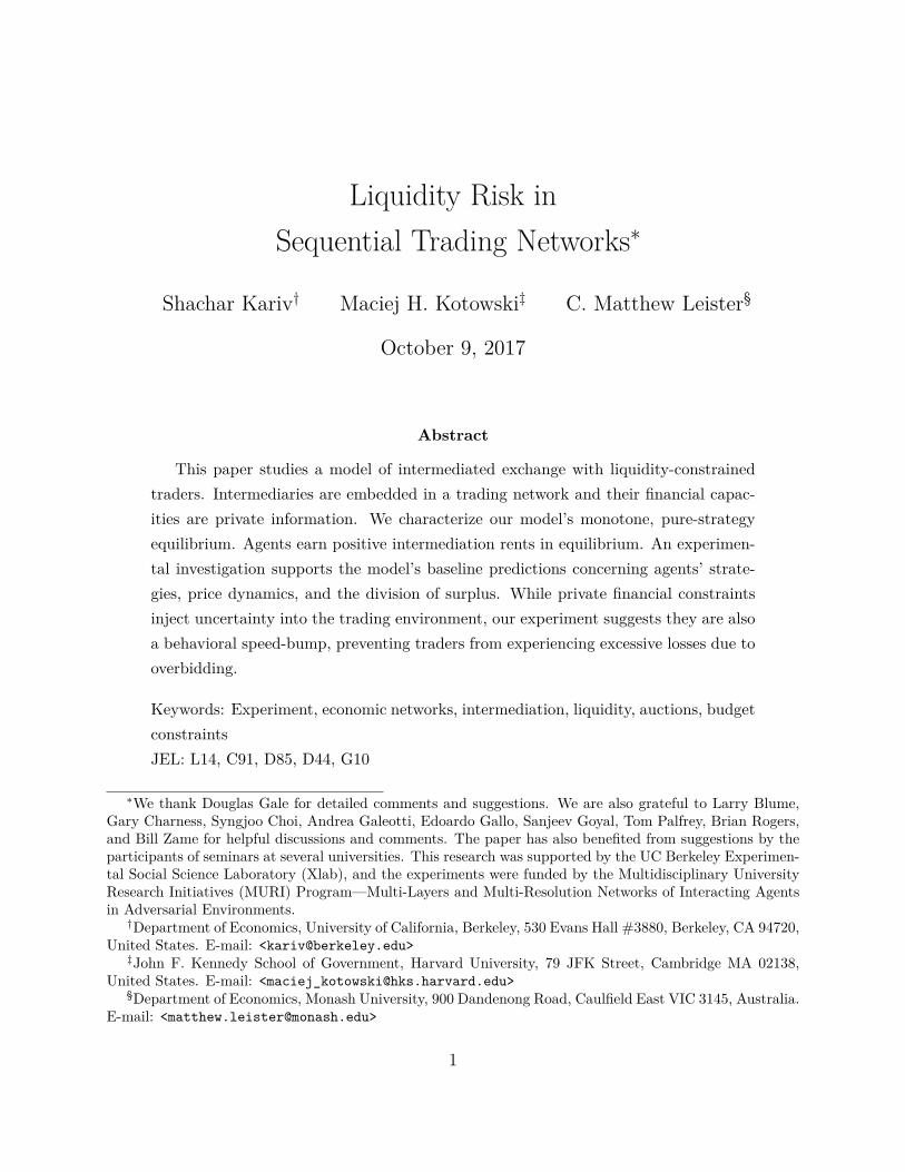
Our model, which builds on Gale and Kariv (2009), is simple, yet rich enough to ad-equately probe the above questions. There is a producer of a good or asset (the “seller”)and a final consumer (the “buyer”).1 We assume that the seller and the buyer cannot tradedirectly. Instead, the asset must pass through a sequence of intermediary traders en routefrom the seller to the buyer. An instance of such a situation is illustrated in Figure 1, withfour intermediary traders. A network specifies the relationships among the agents and deter-mines the feasible transactions among them. If agent i is linked to agent j, then these agentscan trade; otherwise, transactions between them cannot occur. Traders, whose motives arepurely speculative, buy and resell the asset facilitating its passage along links in the networkfrom the seller to the buyer.

The key feature of our model, and where we substantively depart from Gale and Kariv(2009), is that each trader is liquidity or budget constrained. He has limited funds to finance

1Following Gale and Kariv (2009), we call the traded good an “asset.” Depending on the application, itmay represent a financial product or a physical item.

2

Seller

Buyer

Traders

Figure 1: A trading network.

his trading activity. These constraints are private information and inject considerable riskinto the market. A successful trader must anticipate the funds available to his immediatecounter-parties and be mindful of similar constraints elsewhere in the economy. For sim-plicity, we assume that transaction prices are set by a first-price auction. In equilibrium,intermediaries in our economy adopt subtle bidding strategies accounting for the compound-ing financing risks. Average prices systematically rise as the asset nears the final buyer.Traders closer to the buyer benefit from the reduction of uncertainty. They manage togarner a relatively larger share of the surplus than traders further away.

Our model’s simplicity ensures that it can be readily tested empirically in a laboratorysetting. Our experiments confirm the key conclusions from our theoretical analysis. Agentswith ample funds shade their bid relative to their trading budget and intermediaries closerto the final buyer adopt uniformly more aggressive bidding strategies. Consequently, pricesrise and intermediaries closer to the buyer tend to earn higher trading profits. Interestingly,our experiment also identifies a practical disciplinary role played by financial frictions andbudget constraints. In the laboratory, we observe that traders who are flush with resourcestend to experience a mild decline in profits relative to the equilibrium benchmark and toothers. While a lax budget constraint allows a trader greater freedom to pursue his goals, italso allows him to err and overbid with greater frequency. The latter effect often dominates.

This paper is organized as follows. Section 2 briefly reviews the related literature. Welink our study to both theoretical and experimental studies of networked markets and auc-tions. Section 3 introduces our model. The model’s equilibrium analysis is presented inSection 4. We derive several implications concerning intermediary behavior, price dynamics,and welfare. Our experiment’s procedures are summarized in Section 5. Data analysis isperformed in Section 6. Section 7 provides a discussion of our results and our study’s broaderimplications. Section 8 concludes. All proofs are gathered in Section 9. An Online Appendixcontains supplementary material pertaining to our study and experiment.

3

2 Related LiteratureThis paper contributes to literatures on networked markets and auctions. From a theoret-ical point of view, our study is closely related to recent examinations of sequential tradewithin networked economies. This literature builds upon Kranton and Minehart (2001) byincorporating market intermediaries into the trading process. By assumption, buyers andsellers must interact through intermediaries, who facilitate trade while respecting their net-work of relationships. Recent contributions to this literature include Gale and Kariv (2007),Blume et al. (2009), Gale and Kariv (2009), Kotowski and Leister (2014), Choi et al. (2017),Manea (forthcoming), and Condorelli et al. (2017). Condorelli and Galeotti (2015) providea recent survey. Our study complements this growing literature by proposing a new modelof intermediated exchange in the presence of private information about trading ability.

As noted above, our analysis is closest to that of Gale and Kariv (2009), who studya similar class of trading economies. Assuming a complete information setting, Gale andKariv (2009) show that prices converge to the asset’s value and all intermediation rents arequickly competed away. Our study differs in two important ways. Most importantly, westudy an economy where intermediaries hold private information concerning their tradingability, which we model as a budget to bankroll transactions. Second, our price-settingmechanism, a standard first-price auction, is simpler than Gale and Kariv’s protocol, whichinvolves averaging bid and ask prices.2 These departures lead to predictions distinct fromthose advanced by Gale and Kariv (2009). Average prices in our economy rise with successivetransactions and traders enjoy positive intermediation rents.

Other network-based trading games are studied by Charness et al. (2007) and Judd andKearns (2008). The former considers bargaining while the latter considers a trading processwith continuously-updated limit-order books. Choi et al. (2017) examine intermediatedexchange theoretically and in the laboratory focusing on a posted-price mechanism. Theirexperiment highlights the importance of coordination among market intermediaries and therole of “critical traders.” Critical traders enjoy monopoly-like positions in a network allowingthem to extract considerable intermediation rents. Our economy does not feature criticaltraders; instead, we identify an alternative channel allowing intermediaries to earn sustainedprofits in equilibrium. Kosfeld (2004) provides a survey of other laboratory experimentsinvolving networked economies.

2Gale and Kariv (2009) report results from a control treatment where transaction prices equaled only thebid, as in our model. These results are similar to their baseline experiment with the more complex pricingrule. Mindful of this result, we have opted for a simpler pricing rule from the onset. See also Remark 2.

4

Though our focus is on trade in a networked economy, we also contribute to the ex-perimental auction literature. Our experiments incorporate a direct test of Che and Gale’s(1996) model of a first-price auction with private budget constraints. In this model, eachbidder has a one-dimensional type, a private budget constraint above which he cannot bid,and the item for purchase has a commonly-known and fixed value.3 To our knowledge, Cheand Gale’s (1996) model has not been tested in a laboratory before. Anticipating our results,data from our baseline treatment are consistent with the equilibrium that they character-ize. Other experimental investigations of auctions with budget constraints include Kotowski(2010) and Ausubel et al. (2017), albeit they consider environments different from ours.Pitchik and Schotter (1988) examine sequential auctions with budget constraints theoreti-cally and experimentally; however, they consider a setting where multiple goods are sold insequence. In our case, the same good is sold and resold among a sequence of distinct agents.Comprehensive surveys of the experimental auction literature are provided by Kagel (1995)and Kagel and Levin (2016).

3 The ModelIn this section we introduce the model that will inform our experimental analysis. Wecharacterize its equilibrium in the next section.

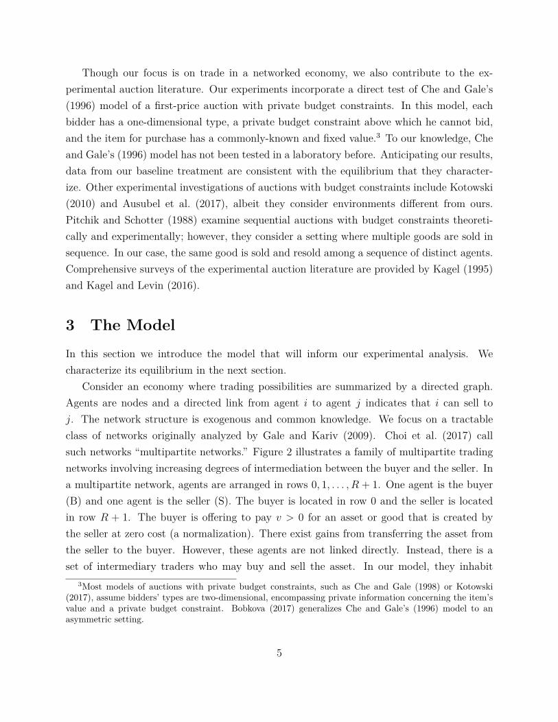
Consider an economy where trading possibilities are summarized by a directed graph.Agents are nodes and a directed link from agent i to agent j indicates that i can sell toj. The network structure is exogenous and common knowledge. We focus on a tractableclass of networks originally analyzed by Gale and Kariv (2009). Choi et al. (2017) callsuch networks “multipartite networks.” Figure 2 illustrates a family of multipartite tradingnetworks involving increasing degrees of intermediation between the buyer and the seller. Ina multipartite network, agents are arranged in rows 0, 1, . . . , R + 1. One agent is the buyer(B) and one agent is the seller (S). The buyer is located in row 0 and the seller is locatedin row R + 1. The buyer is offering to pay v > 0 for an asset or good that is created bythe seller at zero cost (a normalization). There exist gains from transferring the asset fromthe seller to the buyer. However, these agents are not linked directly. Instead, there is aset of intermediary traders who may buy and sell the asset. In our model, they inhabit

3Most models of auctions with private budget constraints, such as Che and Gale (1998) or Kotowski(2017), assume bidders’ types are two-dimensional, encompassing private information concerning the item’svalue and a private budget constraint. Bobkova (2017) generalizes Che and Gale’s (1996) model to anasymmetric setting.

5

S

B

1

(a) A 1× 3 network.

S

B

2

1

(b) A 2× 3 network.

S

B

3

2

1

(c) A 3× 3 network.

Figure 2: A family of multipartite trading networks.

rows 1, . . . , R. Rows are numbered according to their network distance from the buyer.4

Traders, who are risk neutral, do not value the asset per se. Rather they seek to earn profitsby facilitating trades in the network. The network constrains the set of feasible trades asfollows. An agent in row r can purchase the asset from an agent in row r + 1 and can sellthe asset to an agent in row r− 1, as illustrated in Figure 2 with the corresponding directedlinks. As usual, a trader earns profits if he can “buy low” and “(re)sell high.”

The particular trading networks illustrated in Figure 2 feature in our experimental in-vestigation and involve one, two, or three rows of intermediaries. Intuitively, as the distancebetween the buyer and the seller increases, the market’s operation involves a more complexchain of intermediary transactions. For simplicity, we assume that there is a common num-ber N ≥ 2 of intermediary traders in each row. Extending our results to allow for a differentnumber of intermediaries in each row is straightforward and does not change our qualitativeconclusions. In Figure 2, each row has three intermediaries.

All trade occurs via sequential auctions according to the following protocol. When anagent in row r + 1 holds the asset, he organizes a first-price, sealed-bid auction to sell it.Agents in row r participate in the auction by submitting bids. The highest bidder is awardedthe asset and makes a payment equal to his bid. Ties among highest bidders are resolvedwith a uniform randomization. This process continues until the asset reaches the buyer, who(by assumption) pays v for the good.

With the exception of the pricing rule, the model above broadly parallels that of Gale4Our numbering scheme simplifies our equilibrium characterization. Gale and Kariv (2009) follow the

opposite numbering convention.

6

and Kariv (2009). Substantially departing from their setting, we additionally assume thatagents have private information, a common feature of many trading environments. As out-lined in the introduction, we assume that each intermediary trader faces a private budgetconstraint that represents his access to funds or liquidity to finance his trading activity.When attempting to acquire the asset, each trader is constrained to bid less than his privatebudget. This budget has no direct impact on an agent’s payoff; it only describes his feasibleactions.

To model this constraint, we assume that trading budgets are independently and iden-tically distributed according to the cumulative distribution function F . We assume that Fadmits a continuous density, f , with full support on the interval [0, w̄] where 0 < v ≤ w̄.Though straightforward to relax, for analytical brevity we assume that the ratio F (w)/f(w)

is non-decreasing in w. Many common distributions, including the uniform, satisfy this con-dition. As standard, this information structure is common knowledge among all agents inthe economy, though a trader’s realized budget (i.e., his type) is his private information.When there is one row of intermediary traders (R = 1), our model reduces to Che andGale’s (1996) model of a common-value, first-price, sealed-bid auction with private budgetconstraints.

4 Equilibrium Analysis and Model PredictionsWe start by characterizing an equilibrium in monotone, pure strategies. Monotone, purestrategy equilibria are focal in auction-like settings. Che and Gale (1996), whose modelour market generalizes, also focus on such equilibria. While the payment made by thebuyer is fixed by assumption, the value of the asset to traders in rows r ≥ 2 is determinedendogenously. The value of the asset to a row-2 trader, for example, depends on the expectedbids of row-1 traders. Likewise, the value of the asset to a row-3 trader depends directly onthe expected bids of row-2 traders and indirectly on the bids of row-1 traders; and so on.The result of this inductive reasoning is an equilibrium featuring a recursive structure.

To specify the resulting equilibrium strategy, we first define G(w) := F (w)N as thecumulative distribution function (c.d.f.) of the largest of N independent random variables,each with c.d.f. F (w). As usual, g := G′ is the corresponding density.

Theorem 1. Let U1(w) = maxb∈[0,w] F (b)N−1(v − b) and define

b∗1(w) = v − U1(w)

F (w)N−1.

7

For r ≥ 2, define inductively the following expressions:

ν∗r−1 =

∫ w̄

0

b∗r−1(w)g(w) dw (1)

Ur(w) = maxb∈[0,w]

F (b)N−1(ν∗r−1 − b

)(2)

b∗r(w) = ν∗r−1 −

Ur(w)

F (w)N−1(3)

The strategy profile where all traders in row r bid according to the strategy b∗r(w) is theunique, monotone, pure strategy equilibrium of the trading game.

The proof of Theorem 1 follows by induction from the analysis of Che and Gale (1996). Animmediate consequence of the equilibrium’s inductive structure is that the strategy definedin Theorem 1 is independent of the parameter R. That is, if b∗r is the equilibrium biddingstrategy of a row-r trader in a network with R ≥ r rows (and N traders per row), then b∗r

continues to be the equilibrium bidding strategy of a row-r trader in a network with R′ ≥ r

rows (and N traders per row).Before discussing the above equilibrium in greater detail, we present an example paral-

leling our experimental investigation to follow.

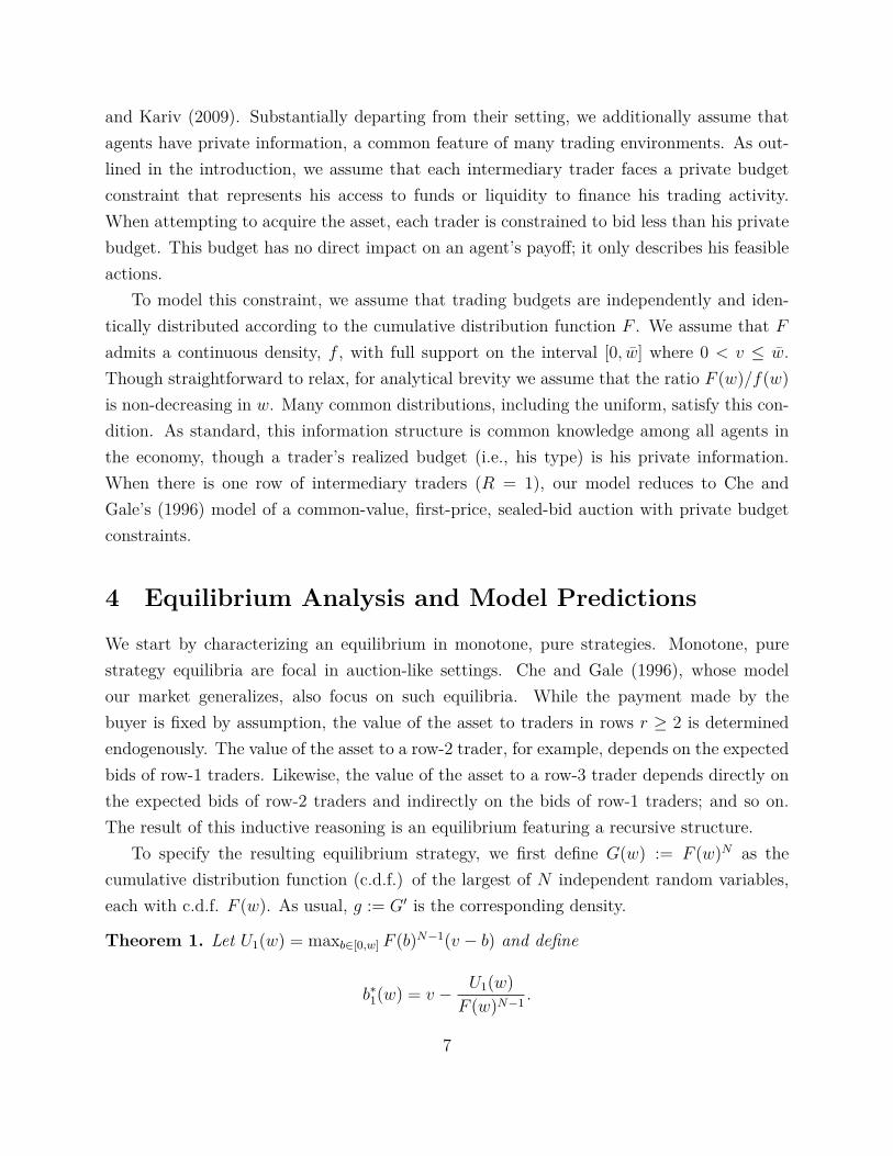
Example 1. Suppose the buyer offers to pay v = 100 for the asset and traders’ budgets areuniformly distributed between 0 and 100. Assume that N = R = 3, as in Figure 2(c). Theequilibrium bidding strategies are illustrated in Figure 3. These bidding strategies are:5

b∗1(w) =

w if w < 67

100− 145000w2 if 67 ≤ w

b∗2(w) =

w if w < 46

70− 50000w2 if 46 ≤ w

b∗3(w) =

w if w < 39

59− 30000w2 if 39 ≤ w

The equilibrium strategy of agents in each row is strictly increasing in w and concave. As agroup, equilibrium strategies are ordered with traders in row 1 submitting the highest bids.

This example nests equilibria from other trading networks as special cases. In particular,5When stating the strategy, we round several values for expositional ease.

8

w

b

20 40 60 80

20

40

60

80b∗1

b∗2

b∗3

100

100

Figure 3: Equilibrium bidding strategies in Example 1.

if R = 1 and N = 3, then the equilibrium strategy is composed only of b∗1. If R = 2 andN = 3, then b∗1 and b∗2 characterize the traders’ equilibrium bidding strategies.

Example 1 suggests several general characteristics of equilibrium behavior in our net-worked market. These conclusions touch on individual-level strategies, price dynamics, andwelfare implications. We summarize these features in three corollaries, which will inform ourexperimental investigation. The first corollary focuses on two striking features of individual-level bidding strategies.

Corollary 1 (Bidding). Consider the equilibrium characterized by Theorem 1.

1. There exists a critical value w∗r such that for all w ≤ w∗

r , b∗r(w) = w. For all w > w∗r ,

b∗r(w) is strictly increasing, concave, and strictly less than w.

9

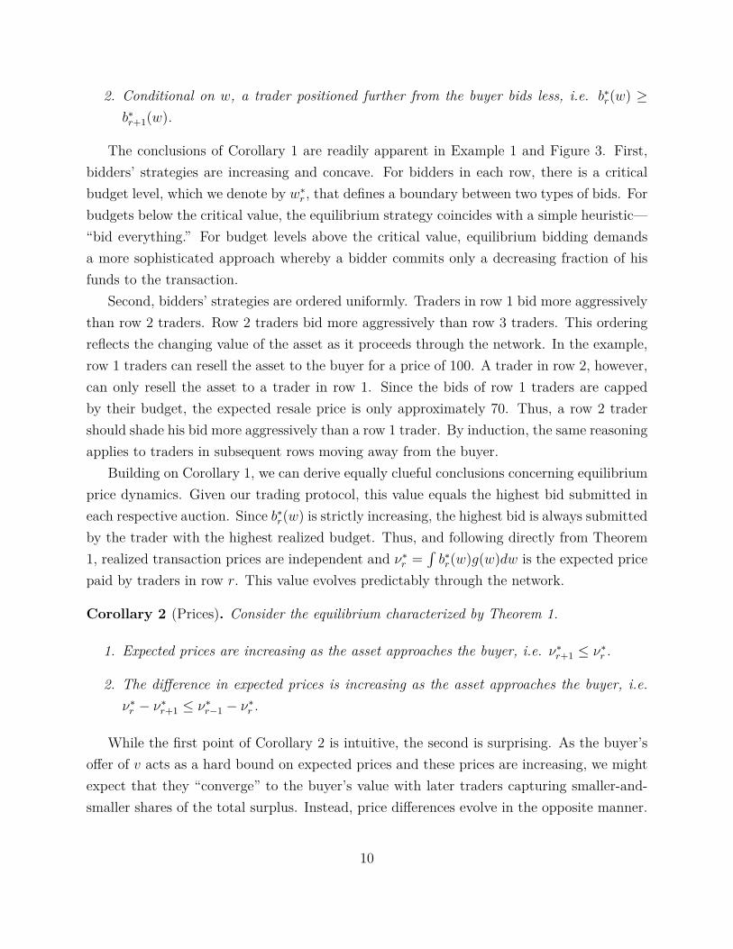
2. Conditional on w, a trader positioned further from the buyer bids less, i.e. b∗r(w) ≥b∗r+1(w).

The conclusions of Corollary 1 are readily apparent in Example 1 and Figure 3. First,bidders’ strategies are increasing and concave. For bidders in each row, there is a criticalbudget level, which we denote by w∗

r , that defines a boundary between two types of bids. Forbudgets below the critical value, the equilibrium strategy coincides with a simple heuristic—“bid everything.” For budget levels above the critical value, equilibrium bidding demandsa more sophisticated approach whereby a bidder commits only a decreasing fraction of hisfunds to the transaction.

Second, bidders’ strategies are ordered uniformly. Traders in row 1 bid more aggressivelythan row 2 traders. Row 2 traders bid more aggressively than row 3 traders. This orderingreflects the changing value of the asset as it proceeds through the network. In the example,row 1 traders can resell the asset to the buyer for a price of 100. A trader in row 2, however,can only resell the asset to a trader in row 1. Since the bids of row 1 traders are cappedby their budget, the expected resale price is only approximately 70. Thus, a row 2 tradershould shade his bid more aggressively than a row 1 trader. By induction, the same reasoningapplies to traders in subsequent rows moving away from the buyer.

Building on Corollary 1, we can derive equally clueful conclusions concerning equilibriumprice dynamics. Given our trading protocol, this value equals the highest bid submitted ineach respective auction. Since b∗r(w) is strictly increasing, the highest bid is always submittedby the trader with the highest realized budget. Thus, and following directly from Theorem1, realized transaction prices are independent and ν∗

r =∫b∗r(w)g(w)dw is the expected price

paid by traders in row r. This value evolves predictably through the network.

Corollary 2 (Prices). Consider the equilibrium characterized by Theorem 1.

1. Expected prices are increasing as the asset approaches the buyer, i.e. ν∗r+1 ≤ ν∗

r .

2. The difference in expected prices is increasing as the asset approaches the buyer, i.e.ν∗r − ν∗

r+1 ≤ ν∗r−1 − ν∗

r .

While the first point of Corollary 2 is intuitive, the second is surprising. As the buyer’soffer of v acts as a hard bound on expected prices and these prices are increasing, we mightexpect that they “converge” to the buyer’s value with later traders capturing smaller-and-smaller shares of the total surplus. Instead, price differences evolve in the opposite manner.

10

Among all intermediaries, traders closest to the buyer capture the greatest share of theexpected total surplus. Of course, part of the total surplus goes to the seller as well.

As expected prices evolve systematically through the trading network, it is natural thattraders’ payoffs behave equally predictably. From the bidding strategy defined in Theorem1, we can conclude that the equilibrium expected payoff of a row-r trader with a budget ofw equals Ur(w), as defined in (2). Indeed, if we rearrange (3), we see that

b∗r(w) = ν∗r−1 −

Ur(w)

F (w)N−1=⇒ Ur(w) = F (w)N−1(ν∗

r−1 − b∗r(w)).

Conditional on acquiring the asset, a trader earns an expected return of ν∗r−1 − b∗r(w), the

difference between the expected resale price and his bid. The probability with which heacquires the asset equals F (w)N−1, which is simply the probability that all others in his rowhave a budget less than w and bid less than b∗r(w) in equilibrium. With this description ofpayoffs, we can conclude the following.

Corollary 3 (Payoffs). Consider the equilibrium characterized by Theorem 1. Define Ur(w)

as in (2) and define w∗r as in Corollary 1.

1. Ur(w), is strictly increasing in w for all w ≤ w∗r . For all w > w∗

r , Ur(w) is constantand equal to Ur(w) = F (w∗

r)N−1(ν∗

r−1 − w∗r).

2. Conditional on w, expected payoffs are increasing as the distance to the buyer decreases,i.e. Ur+1(w) ≤ Ur(w).

Corollary 3 shows that traders’ type-contingent expected payoffs differ systematicallythrough the network. Greater expected payoffs are earned by traders closer to the buyer.As all traders are ex ante identical except for their position in the network, this impliesthat unconditional expected payoffs are also greatest for traders closer to the buyer. Despitethe analogous network topology, these observations contrast with the conclusions of Galeand Kariv (2009), who argue that intermediation rents are entirely competed away. In oursetting, the presence of private information ensures that intermediation rents remain positive.

Remark 1. Our analysis and experiment focus on the model’s symmetric, monotone, pure-strategy equilibrium, which is both intuitive and focal. Our model also admits many mixed-strategy and non-monotone equilibria. These equilibria replicate the bid distribution inducedby the strategies defined in Theorem 1. Intuitively, since traders with high budgets areindifferent among a range of bids (Corollary 3), their bidding strategies can be “rearranged”

11

without upsetting the equilibrium provided the overall bid distribution remains unchanged.We elaborate on this point in Online Appendix A. Importantly, many of our theoreticalconclusions depend only on the bid distribution; hence, they are robust across equilibria.

Remark 2. A further extension of our setup introduces reserve prices into the pricing protocol.Under this scheme, an agent currently selling the asset could specify a minimum acceptablebid. It is straightforward to extend the analysis of Che and Gale (1996), and thus Theorem1, to allow for reserve prices. Generally, the optimal (and equilibrium) reserve price dependson the economy’s parameters. In Example 1, which parallels our experimental study, therevenue-maximizing reserve price is zero for all traders. The supporting intuition is asfollows. Traders with low budgets “bid everything” in equilibrium and a small reserve priceonly screens them out from the auction. A large reserve price can potentially increase thesale price, but the reduction in sale probability dominates. Hence, expected payoffs decline.Given the optimality of a zero reserve price in our experiment, we have suppressed their rolein our analysis and model.

4.1 A Practical Extension: Limited Liability

Several practical considerations complicate the direct translation of the preceding model toa laboratory setting. One difficulty is that an intermediary trader may incur an ex post loss.With the exception of traders in row 1, it is possible that a trader pays more for the assetthan he subsequently receives from a downstream counter-party. Standard experimentalprotocols and laboratory rules (including ours) do not allow a subject to incur a financialpenalty in a study. Numerous methods have been employed in the literature to address thiscommon concern, sometimes with mixed effects.6 A simple method, which we follow in ourexperiment, involves introducing a limited-liability constraint. Specifically, a trader can beprotected from loss by computing his earnings as

Earnings = max

Resale Price− Purchase Price︸ ︷︷ ︸Trading Profits

, 0

. (4)

Gale and Kariv (2009) compute earnings in their experiment with the same formula. Theyargue that (4) can be interpreted as a compensation scheme for a professional trader whoenjoys bonuses when trading profits are positive, but earns constant wages otherwise.

6This concern also arises in studies of common-value auctions due to the winner’s curse. See Kagel (1995)for a survey.

12

When earnings are computed according to (4), traders’ incentives change relative to ouroriginal model. Since agents are protected from a loss, intuition suggests that equilibriumbidding ought to be more aggressive. In Online Appendix B we provide an equilibriumcharacterization in our economy, analogous to Theorem 1, when (4) defines traders’ payoffs.Though considerably less tractable than the baseline model, the equilibrium can again bedefined inductively. Equilibrium bidding strategies can no longer be expressed in closedform; however, they can be readily computed numerically in standard examples.

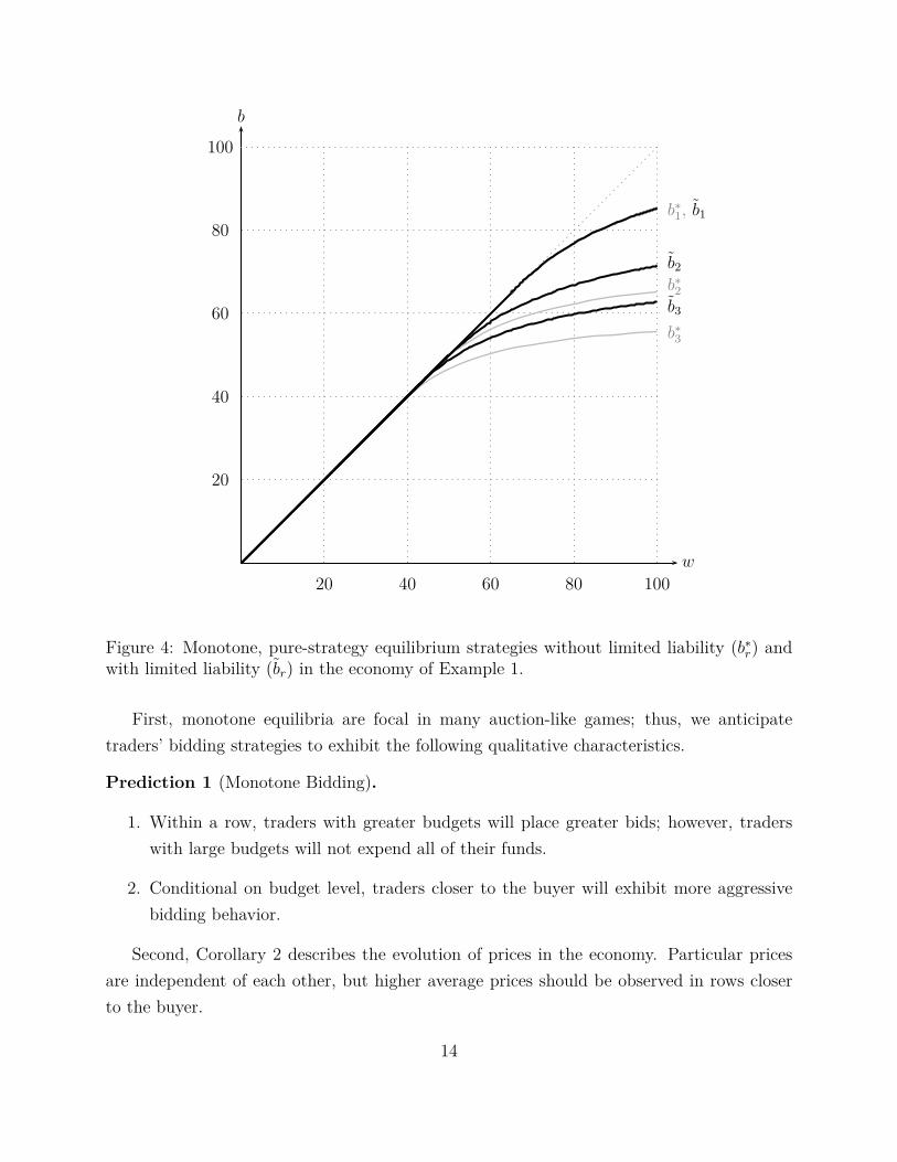
To gauge the impact of limited liability, in Figure 4 we illustrate the equilibrium strategiesfrom Example 1 when earnings are instead computed according to formula (4). Recallthat the example featured three rows of traders, with three traders per row. Budgets wereuniformly distributed between 0 and 100. The asset’s value to the final buyer was 100.(These parameters are identical to those employed in our experiment.) In the figure, weillustrate the equilibrium strategies in the presence of limited liability as dashed curves andlabel them as b̃r(·). For comparison, the figure also illustrates the equilibrium strategies fromour baseline model without limited liability, denoted by b∗r(·). The strategy of row 1 tradersis unaffected by the introduction of limited liability since the buyer always offers more forthe asset than the highest possible bid. Thus, b̃1(w) = b∗1(w). As expected, traders in rows2 and 3 adopt more aggressive postures. They are willing to bid more since the down-siderisk associated with overpaying is mitigated by formula (4). Consequently, b̃2(w) ≥ b∗2(w)

and b̃3(w) ≥ b∗3(w), as illustrated in Figure 4. Paralleling our baseline analysis, for each rowr we define w̃r as the critical budget level such that b̃r(w) = w for all w < w̃r and b̃r(w) < w

for all w > w̃r. With limited liability, the critical values (w̃r) are 43.5, 50.5, and 67. Underits original specification, the critical values (w∗

r) in Example 1 are 39, 46, and 67.Since limited liability affects bidding in a measured manner, the qualitative conclusions

outlined in Corollaries 1–3 continue to obtain. The continued applicability of Corollary 1 isapparent in Figure 4. Given the example’s parameterization, Corollaries 2–3 can be easilyverified, either analytically or numerically. Since many of our original conclusions continueto apply, the limited liability constraint provides a practical, minimally invasive compromisein implementing our experimental market.

4.2 Predictions

We conclude our theoretical analysis by translating our formal results into a set of empiricalpredictions that will form the basis of our experimental investigation. These predictionsdraw on Theorem 1, Corollaries 1–3, and our extension to the case of limited liability.

13

w

b

100

100

20 40 60 80

20

40

60

80

b∗2

b∗3

b∗1, b̃1

b̃2

b̃3

Figure 4: Monotone, pure-strategy equilibrium strategies without limited liability (b∗r) andwith limited liability (b̃r) in the economy of Example 1.

First, monotone equilibria are focal in many auction-like games; thus, we anticipatetraders’ bidding strategies to exhibit the following qualitative characteristics.

Prediction 1 (Monotone Bidding).

1. Within a row, traders with greater budgets will place greater bids; however, traderswith large budgets will not expend all of their funds.

2. Conditional on budget level, traders closer to the buyer will exhibit more aggressivebidding behavior.

Second, Corollary 2 describes the evolution of prices in the economy. Particular pricesare independent of each other, but higher average prices should be observed in rows closerto the buyer.

14

Table 1: Experimental sessions and treatments.

NetworkType

Number ofSessions

TotalSubjects

DecisionObservations

AverageEarnings ($)*

1× 3 1 30 1,500 26.042× 3 2 72 3,600 24.513× 3 3 90 4,500 24.03

* Reported earnings include the $5 show-up fee and the $10 participation fee paid atthe experiment’s conclusion.

Prediction 2 (Prices). Average prices paid by intermediary traders in different rows exhibitan upward trend as the asset approaches the buyer. The gap between purchase and resaleprices is increasing as the asset approaches the buyer.

Our final prediction recasts Corollary 3, establishing comparative statics on traders’welfare and payoffs within and across rows.

Prediction 3 (Payoffs).

1. Within a row, average intermediary profits are increasing when trading budgets arelow and constant when they are high.

2. Conditional on his budget, a trader closer to the buyer earns higher average payoffs.

While Prediction 1 directly builds on the monotone, pure-strategy equilibrium, Predic-tions 2 and 3 apply to the large family of (possibly asymmetric) equilibria, as noted inRemark 1 above. Finally, as explained above, these predictions continue to apply even ifearnings are subject to a limited liability constraint.

5 Experimental Design and ProceduresIn our experiment, we consider a family of networks to test our three main predictions. Table1 provides a summary. First, the 1×3 network allows us to examine the within row elementsof Predictions 1.1 and 3.1. This network, which corresponds to a test of Che and Gale’s(1996) model of a common-value, first-price auction with private budget constraints, allowsus to identify any dependencies in agents’ bids and payoffs on budgets without introducingthe confound of network depth. The 1 × 3 network is insufficient to probe the price andwelfare dynamics across rows. Thus, we also consider the 2 × 3 network and the 3 × 3

15

networks, having two and three layers of intermediaries, respectively, between the buyer andthe seller. These more complex networks also provide a forum to ascertain the robustnessof our within-row conclusions. The monotonicity, concavity, and welfare conclusions applyto these cases as well. To ensure comparability, we maintain the same level of competitionacross treatments. Thus, each row always has three intermediary traders.

Six experimental sessions were conducted at the Experimental Social Science Laboratory(Xlab) at the University of California, Berkeley. We employed the experimental computerprogram developed by Gale and Kariv (2009) and our experimental procedures follow their’sclosely. Subjects were recruited from the undergraduate and graduate student bodies at theuniversity. No subject participated in more than one session. At the start of each session,subjects were given ample time to silently read the experiment’s instructions. We reproducea sample of these instruction in Online Appendix B. The instructions were then read aloudby an administrator. Subjects’ questions, if any, were publicly addressed. Each session lastedroughly one hour and thirty minutes. Each subject received a payment of $5 for showingup at the experiment on time. At the experiment’s conclusion, each subject received anadditional payment of $10 for participating in and completing the experiment plus theirwithin-experiment earnings or trading profits. We describe the calculation of trading profitsbelow. Total compensation for participation in the experiment ranged from $15 (the subjectearned only the show-up and participation fees) to $87.90 (the subject earned the show-upand participation fees plus $72.90 in trading profit). Within the experiment, we refer tounits of currency using the neutral term “tokens.”

Each of six sessions consisted of 50 independent trading rounds. Subjects assumed therole of intermediaries and each round mimicked our model’s operation. The buyer and theseller were modeled by the computer. The network structure was held fixed throughout asession and was clearly explained to the subjects. Each subject was randomly assigned bythe computer to one row of the network. These assignments were privately observed by thesubjects, and were held constant throughout the experiment’s duration. At the beginningof each trading round, the computer randomly formed networks by assigning subjects totheir respective row in a network. Subjects faced the same probability of being placed toany network and to any node position within their preassigned row. Thus, subjects wereunaware of the identities of others in their network in each round.

Upon observing their position in the network and immediately prior to each round ofplay, each subject was informed of his trading budget for that round. This budget, calledthe “token endowment” within the experimental platform, was randomly and uniformly

16

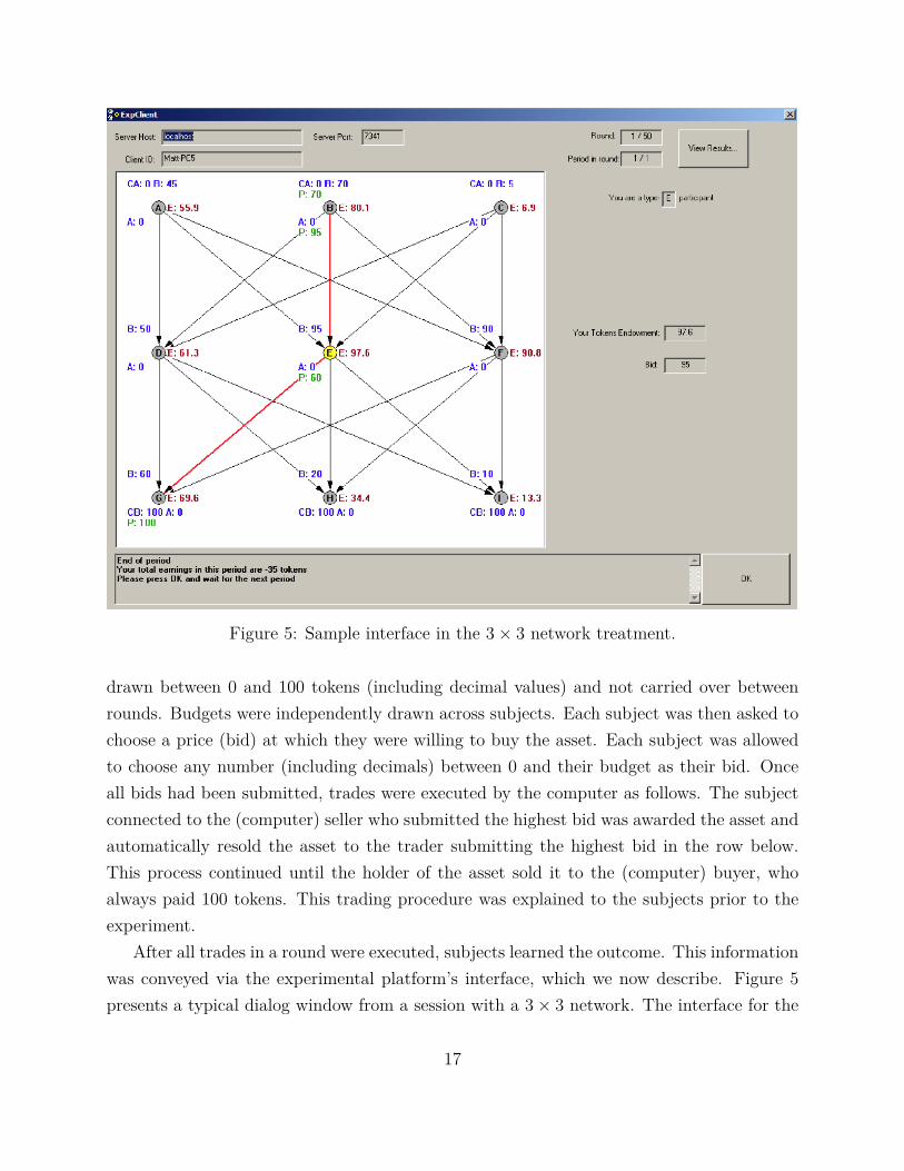
Figure 5: Sample interface in the 3× 3 network treatment.

drawn between 0 and 100 tokens (including decimal values) and not carried over betweenrounds. Budgets were independently drawn across subjects. Each subject was then asked tochoose a price (bid) at which they were willing to buy the asset. Each subject was allowedto choose any number (including decimals) between 0 and their budget as their bid. Onceall bids had been submitted, trades were executed by the computer as follows. The subjectconnected to the (computer) seller who submitted the highest bid was awarded the asset andautomatically resold the asset to the trader submitting the highest bid in the row below.This process continued until the holder of the asset sold it to the (computer) buyer, whoalways paid 100 tokens. This trading procedure was explained to the subjects prior to theexperiment.

After all trades in a round were executed, subjects learned the outcome. This informationwas conveyed via the experimental platform’s interface, which we now describe. Figure 5presents a typical dialog window from a session with a 3× 3 network. The interface for the

17

other network structures was similar. The subject’s position in their network is displayedin the large square window at the left of the screen. Upon completion of a given round,this window also displayed that round’s price and trading information. The “View Results”button in the screen’s top-right corner allowed the subject to view the price and tradinghistory from each previous trading round they participated in. The subject entered his orher bid in the Bid field at the right of the screen. The subject’s budget was displayed inthe Token Endowment field, immediately above the Bid field. After each round of bidding,each subject was informed of others’ bids and budgets. They were also shown the sequenceof executed trades and the associated prices, as illustrated in Figure 5. Provision of thisinformation ensured that subjects trusted and understood the trading protocol and pricingsystem. After each subject clicked “OK,” the next trading round began.

Earnings in the experiment were determined as follows. At the end of the session, thecomputer randomly selected one trading round. Each round had an equal probability ofbeing chosen. The subjects were then paid based on that round’s earnings. To compute finalpayments, tokens were converted into dollars at a 1-for-1 exchange rate. If a subject did nottrade in the selected round, his or her trading profits were zero. The subject received only the$5 show-up fee and $10 participation fee. If a subject did trade in the selected round, he orshe received the show-up and participation fees plus any earnings from the selected round.These earnings were computed according to formula (4), which incorporated the limitedliability constraint. As explained above, use of this payment scheme ensured subjects didnot incur a financial penalty; it was also used by Gale and Kariv (2009).7 Subjects wereinformed of the earnings formula as part of the experiment’s instructions.

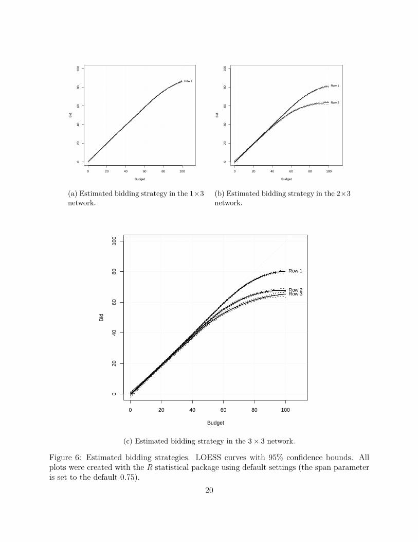
6 Data Analysis and ResultsAs a starting point for our data analysis, we examine bidder behavior. In Figure 6 weplot LOESS curves8 (and 95% confidence bounds) summarizing average bids submitted by

7An alternative experimental design could have endowed bidders with a “buffer” budget of tokens fromwhich trading losses could be deducted. The buffer could have been chosen to be sufficiently large to ensurethat ex post losses are extremely unlikely. We decided against such a design due to its added cost andcomplexity. There is a risk of confusion between the buffer budget and the particular budget constraintin a particular round. Furthermore, loss-aversion may become more salient as a behavioral confound. Webelieve the present design is more closely aligned with our original model and we can account for the payoffformula’s equilibrium consequences directly, as explained in Section 4.1.

8LOESS is a standard non-parametric regression procedure, which fits a local polynomial regression to(in our case) bivariate data. See Fox (2008) for a practical discussion of this and related methods.

18

traders in each row as a function of their budget.9 We group our estimates by network type,but we pool across sessions and bidders.10 In each successive panel, we consider increasinglycomplex networks, with the 3× 3 network presented in panel (c).

Two features of the fitted curves stand out. First, the estimates exhibit the anticipatedmonotonicity and concavity predicted by our theoretical analysis. Across networks, tradersbid their entire budget when it is low. High budget traders do not commit all of their fundsto the auction. Instead, they shade their bid resulting in a concave bidding function. Second,the fitted curves conform to the predicted ordering. Row 1 traders uniformly outbid theirrow 2 and row 3 counterparts. Moreover, in the 3×3 treatment, row 2 traders outbid tradersin row 3. The associated confidence bounds overlap only at extreme values where estimatesare necessarily less precise, due to fewer observations.

Result 1 (Bidding). Across networks, traders’ bids are increasing in their budget level,even when budgets are not a binding constraint. Traders with low budgets bid all of theiravailable funds to acquire the asset. Traders with ample funds reduce their bid relative tothe their budget. Across networks, intermediaries closer to the final buyer adopt uniformlymore aggressive bidding strategies.

As for price dynamics, in Table 2 we report descriptive statistics concerning the pricespaid by traders to acquire the asset. The table summarizes these values conditional on thenetwork structure and on the row, though the values are pooled across sessions and tradingrounds. For example, a trader in a 1 × 3 network who successfully acquired the asset fromthe seller, paid 70.71 tokens on average. The median price paid was higher, 75 tokens, andthe standard deviation was 17.16 tokens. Similar statistics are reported for other networkson a row-by-row basis.

A first-order feature apparent from Table 2 is the trend in average prices as the assetapproaches the buyer. In a 2 × 3 network, the price paid by a row 1 trader to acquire theasset (from a row 2 trader) is on average 10.5 tokens greater than the price paid by a row2 trader to acquire the asset (from the seller). In a 3 × 3 network, a row 1 trader paid onaverage 7.18 tokens more than a row 2 trader. A row 2 trader paid on average 2.57 tokens

9All of our estimates and data analysis use the full data sample. As a robustness check, we have repeatedour estimates dropping the first 10 and 25 rounds from each session to account for the possibility of learning.The results of this exercise were not substantively different from the estimates based on the full sample. Ourresults support Gale and Kariv’s (2009) conclusion that subjects appear to adapt quickly to this type oftrading environment.

10In Online Appendix D we estimate a parametric model controlling for subject-level effects. The conclu-sions are entirely analogous to those presented here. Pooling by session yields similar conclusions.

19

0 20 40 60 80 100

020

4060

8010

0

Budget

Bid

Row 1

(a) Estimated bidding strategy in the 1×3network.

0 20 40 60 80 100

020

4060

8010

0

Budget

Bid

Row 2

Row 1

(b) Estimated bidding strategy in the 2×3network.

0 20 40 60 80 100

020

4060

8010

0

Budget

Bid

Row 3Row 2

Row 1

(c) Estimated bidding strategy in the 3× 3 network.

Figure 6: Estimated bidding strategies. LOESS curves with 95% confidence bounds. Allplots were created with the R statistical package using default settings (the span parameteris set to the default 0.75).

20

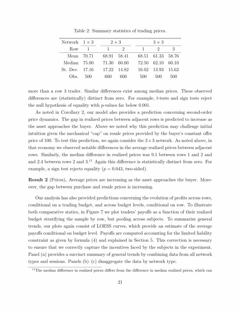
Table 2: Summary statistics of trading prices.

Network 1× 3 2× 3 3× 3

Row 1 1 2 1 2 3Mean 70.71 68.91 58.41 68.51 61.33 58.76

Median 75.00 71.30 60.00 72.50 62.10 60.10St. Dev. 17.16 17.22 14.82 16.02 13.93 15.62

Obs. 500 600 600 500 500 500

more than a row 3 trader. Similar differences exist among median prices. These observeddifferences are (statistically) distinct from zero. For example, t-tests and sign tests rejectthe null hypothesis of equality with p-values far below 0.001.

As noted in Corollary 2, our model also provides a prediction concerning second-orderprice dynamics. The gap in realized prices between adjacent rows is predicted to increase asthe asset approaches the buyer. Above we noted why this prediction may challenge initialintuition given the mechanical “cap” on resale prices provided by the buyer’s constant offerprice of 100. To test this prediction, we again consider the 3×3 network. As noted above, inthat economy we observed notable differences in the average realized prices between adjacentrows. Similarly, the median difference in realized prices was 9.1 between rows 1 and 2 andand 2.4 between rows 2 and 3.11 Again this difference is statistically distinct from zero. Forexample, a sign test rejects equality (p = 0.043, two-sided).

Result 2 (Prices). Average prices are increasing as the asset approaches the buyer. More-over, the gap between purchase and resale prices is increasing.

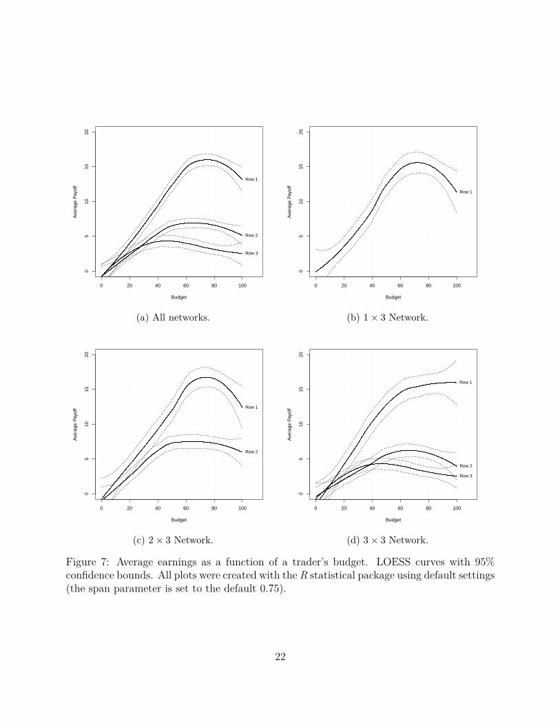
Our analysis has also provided predictions concerning the evolution of profits across rows,conditional on a trading budget, and across budget levels, conditional on row. To illustrateboth comparative statics, in Figure 7 we plot traders’ payoffs as a function of their realizedbudget stratifying the sample by row, but pooling across subjects. To summarize generaltrends, our plots again consist of LOESS curves, which provide an estimate of the averagepayoffs conditional on budget level. Payoffs are computed accounting for the limited liabilityconstraint as given by formula (4) and explained in Section 5. This correction is necessaryto ensure that we correctly capture the incentives faced by the subjects in the experiment.Panel (a) provides a succinct summary of general trends by combining data from all networktypes and sessions. Panels (b)–(c) disaggregate the data by network type.

11The median difference in realized prices differs from the difference in median realized prices, which can

21

0 20 40 60 80 100

05

1015

20

Budget

Ave

rage

Pay

off

Row 2

Row 1

Row 3

(a) All networks.

0 20 40 60 80 100

05

1015

20Budget

Ave

rage

Pay

off

Row 1

(b) 1× 3 Network.

0 20 40 60 80 100

05

1015

20

Budget

Ave

rage

Pay

off

Row 2

Row 1

(c) 2× 3 Network.

0 20 40 60 80 100

05

1015

20

Budget

Ave

rage

Pay

off

Row 3

Row 2

Row 1

(d) 3× 3 Network.

Figure 7: Average earnings as a function of a trader’s budget. LOESS curves with 95%confidence bounds. All plots were created with the R statistical package using default settings(the span parameter is set to the default 0.75).

22

Agreeing with Prediction 3, traders closer to the buyer enjoy higher average payoffsconditional on realized budget. Empirically, the sole exception to this general pattern occursat low budget levels. Traders with low budgets always have a small chance of successfullyacquiring the asset; hence, payoffs are (unsurprisingly) uniformly low. When budgets arehigh, however, the ordering of traders’ payoffs is evident and robust. It appears in theaggregate data and on a network-by-network basis.

Though the evolution of payoffs across rows provides a definite comparison, the evolutionof payoffs within a row is more subtle. Recalling Corollary 3 and Prediction 3, we anticipatethat average payoffs will be increasing when budgets are low and constant when budgets arehigh. The former effect is apparent in all panels of Figure 7. The latter effect, however,appears to not be a feature of the data. Curiously, average payoffs exhibit a mild downwardtrend at high budget level. This effect is evident in panel (a) and remains a persistent featureat finer scales.

To evaluate the significance of this apparent downward trend, we first draw on our theo-retical model to aid in sample selection. Restricting the sample to budget realizations abovew̃r, we regress trader’s earnings on their realized budget. (Recall that w̃r denotes the cut-offvalue after which traders bid less than their budget in equilibrium and expected payoffs are intheory constant.) By Corollary 3 and Prediction 3, the resulting regression estimates shouldbe zero. Tables 3 and 4 report the outcomes of these calculation controlling for subject fixedeffects. For comparison, Table 3 corresponds to Figure 7, panel (a), and Table 4 correspondsto Figure 7, panels (b)–(d).

In Table 3 we identify a mild, though statistically significant, negative correlation betweenrealized budgets and payoffs. Thus, beyond the w̃r threshold, an increase in a trader’s budgetis associated with a decline in average earnings. For example, increasing the budget of arow 1 trader from 67 to 100, thereby removing all constraints on his bid, reduces his averagepayoff by about 3 tokens (dollars). Similar declines affect row 2 and row 3 traders. This effectappears despite the limited liability constraint present in our experiment, which precludestrading losses from pulling-down realized payoffs further.12 Table 4 repeats the estimatesof Table 3, but on more disaggregated samples. Across all specifications, the consistentlynegative point estimates of the budget coefficient corroborate the presence of a downwardtrend, though some estimates lose statistical significance.

be computed directly from Table 2.12Neglecting the limited liability constraint maintains the payoff ordering but significantly reinforces the

downward trend in the payoffs of row 2 and row 3 traders with high budgets. Therefore, the correction forearnings formula (4) is important.

23

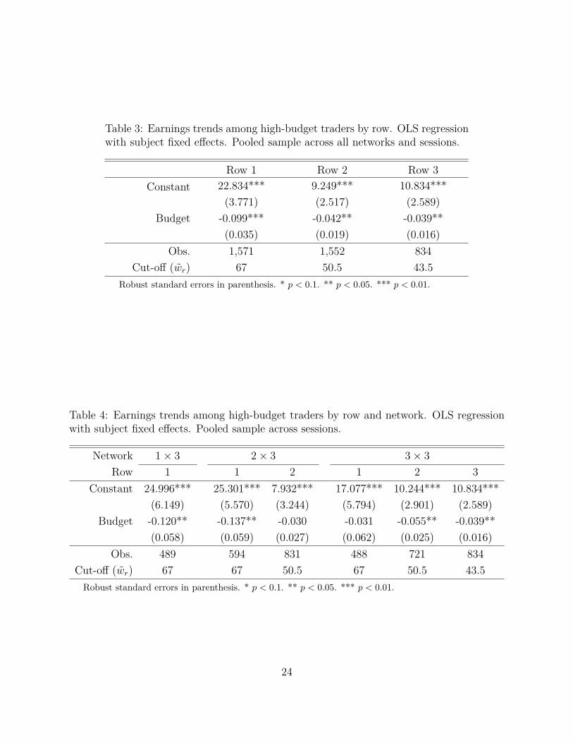
Table 3: Earnings trends among high-budget traders by row. OLS regressionwith subject fixed effects. Pooled sample across all networks and sessions.

Row 1 Row 2 Row 3Constant 22.834*** 9.249*** 10.834***

(3.771) (2.517) (2.589)Budget -0.099*** -0.042** -0.039**

(0.035) (0.019) (0.016)Obs. 1,571 1,552 834

Cut-off (w̃r) 67 50.5 43.5Robust standard errors in parenthesis. * p < 0.1. ** p < 0.05. *** p < 0.01.

Table 4: Earnings trends among high-budget traders by row and network. OLS regressionwith subject fixed effects. Pooled sample across sessions.

Network 1× 3 2× 3 3× 3

Row 1 1 2 1 2 3Constant 24.996*** 25.301*** 7.932*** 17.077*** 10.244*** 10.834***

(6.149) (5.570) (3.244) (5.794) (2.901) (2.589)Budget -0.120** -0.137** -0.030 -0.031 -0.055** -0.039**

(0.058) (0.059) (0.027) (0.062) (0.025) (0.016)Obs. 489 594 831 488 721 834

Cut-off (w̃r) 67 67 50.5 67 50.5 43.5Robust standard errors in parenthesis. * p < 0.1. ** p < 0.05. *** p < 0.01.

24

We can rationalize the observed downward trend in payoffs with a simple behavioral argu-ment. In our model, the blessing of a high budget comes with the curse of more opportunitiesfor error. An intermediary with a tight budget constraint faces a relatively straightforwardproblem in formulating his bid. With high probability the asset’s resale value will exceedhis budget. Bidding up to his budget constraint provides a simple, focal heuristic strategyguaranteeing considerable upside in the (admittedly, unlikely) event that he is the winner.Limited liability shields him from losses while the budget constraint provides protection fromoverbidding.

The problem faced by a high-budget trader is more complex. Agents with high budgetshave sufficient funds to compete for the asset. Hence, they must be more careful in balancingthe probability of winning the auction and the surplus derived from resale. This introducesadditional channels for error or misperception to enter into the bid-formulation process. Ahigh budget provides no mechanical backstop preventing overbidding, thereby allowing thesemiscalculations and temptations to filter into the trading game.

Result 3 (Trader Profits). On average, intermediaries closer to the buyer earn higher tradingprofits. Average profits are initially increasing in a trader’s budget. When a trader’s budget isrelatively large, a further increase in his budget is associated with a mild, though statisticallysignificant, decline in earnings.

7 Discussion and InterpretationAs with all market experiments, we build our analysis around a stripped-down theoreticalmodel that we subsequently test with a particular population. Neither the trading platformnor the university-student subject pool perfectly replicates the “real world.” Of course,concerns regarding an experiment’s external validity are not new; see Chapters 14–20 ofFréchette and Schotter (2015) for an extensive survey. Our analysis studies general principlesof market operation. Thus, echoing Kessler and Vesterlund (2015), we believe the qualitativeinsights of our study will generalize to related non-laboratory environments even though thequantitive estimates are specific to our model and experiment. Generalizable insights fromour analysis include (i) the coordination on an equilibrium that is monotone in financialcapacity,13 (ii) the payoff advantage enjoyed by intermediaries closer to a final buyer or

13We note, additionally, that equilibria are monotone within each transaction episode (i.e. auction) andacross transactions occurring within the same market.

25

consumer, and (iii) the disciplinary benefit of budget constraints observed in the laboratory,which we interpret as preventing behavioral errors.14

Below we explain how two elements of our model, the multipartite network structure andthe private budget constraints, relate to features beyond the laboratory environment.

Multipartite Trading Networks

A characteristic of our setting is the network structure. The number of rows—the parameterR—describes the prevailing depth of intermediation in the market. It counts the numberof intermediaries involved in moving assets from sellers to buyers. Different markets willexhibit different values of this parameter. In Kranton and Minehart (2001), for example,R = 0 as buyers and sellers are linked directly. Often, however, R may assume a relativelylarge value. For example, Li and Schürhoff (2014) have recently documented the presenceof long chains of successive intermediaries in over the counter (OTC) trades of municipalbonds. They note that approximately a quarter of transactions between buyers and sellersin this market involve multiple intermediaries. Describing these transactions, they write:

[L]onger chains start with a dealer purchasing a bond from a customer, followedby one or several interdealer trades that move the bond from the head dealerto the tail dealer, and end with the tail dealer selling the bond to one or morecustomers. (Li and Schürhoff, 2014, p. 14)

This process closely aligns with our framework.Beyond OTC markets, our network structure parallels some of the directed intermedia-

tion observed in financial systems and supply chains (Spulber, 1996). As large institutionssave and consumers borrower, for example, financial intermediaries, i.e. banks and dealers,facilitate the movement of funds between wholesale and retail markets. Similarly, buyerfinancing is a prominent concern in many export industries, which often depend on inter-mediaries to fund complex transactions and to facilitate the movement of physical goods.Though stylized, we believe our model provides some insight to the strategic dynamics atplay in these applications.

Multipartite networks also offer insights regarding more complex economies by focusingon local interactions among agents. They can be interpreted as a small neighborhood withina larger economy where a few agents enjoy a dense set of relationships among each other.

14This behavioral disciplinary effect complements the use of budget constraints to solve a principal-agentproblem in an auction environment (Burkett, 2016; Ausubel et al., 2017).

26

Under this paradigm, the non-strategic seller and the buyer can be interpreted as metaphorsfor (not modeled) upstream and downstream markets, respectively.

Private Budget Constraints

Private information plays a central role in our model and in our experimental study. In-troducing private information on top of an economic network, however, compounds theenvironment’s complexity. We focus on the case of private budget constraints because theyarise naturally in many markets and they capture, sometimes in reduced form, many types ofmarket uncertainty. Beyond its literal interpretation as a hard financial constraint, a budgetconstraint may also reflect an economic opportunity-cost of funds.

More abstractly, a reinterpreted private budget may capture behavioral constraints notdirectly related to financial capacity. For example, it may capture a trader’s relative statusin the network. A trader with perceptions of weak ties to resale markets—represented by alow realized “budget”—may be unwilling or unable to commit a large sum to a particularinteraction. In our economy, such low-budget traders tend to earn relatively large profitsconditional on trading successfully; however, they trade with relatively low frequency.

8 ConclusionWe study a decentralized market with financing risk and a multipartite network structure,focusing on intermediary behavior. In our economy, (average) transaction prices rise withsuccessive transactions and intermediaries positioned closer to the buyer enjoy greater ex-pected profits. We find strong evidence supporting these theoretical predictions in our labo-ratory experiments. In the lab, we also identify a mild negative correlation between expectedprofits and subjects’ trading budgets, conditional on budgets being relatively high. That is,liquidity-rich traders tend to overbid. This trend is observed across rows. Tighter budgetconstraints appear to mitigate this behavioral tendency. Thus, budgets have a disciplinaryrole in markets, preventing excessively costly “trembles” or “errors.”

While the implication of private liquidity risk has been well-studied in centralized ex-changes,15 the pricing and distributional implications of liquidity risk in decentralized mar-kets is much less understood. Our analysis provides clear predictions, substantiated byexperimental data, concerning the compounding of risk in a decentralized market. We alsodescribe the strategies adopted by market participants in response to its presence. Analyzing

15See Foucault et al. (2013) for a recent survey.

27

specific policy interventions, such as liquidity injections that target trading positions withinthe market, offers a promising avenue for future research.

9 ProofsProof of Theorem 1. The proof is by induction. The base case for b∗1 follows immediatelyfrom Che and Gale (1996). For r > 1, the expected resale value of the asset is ν∗

r−1. Applyingthe argument from Che and Gale (1996) to a first-price auction with a common value of ν∗

r−1

confirms that b∗r(w) is an equilibrium strategy for intermediaries in row r. Their argumentapplies as b∗r(w) is independent of the asset’s price history.

Proof of Corollary 1.

1. Since F (w)/f(w) is increasing, F (w)N−1(ν∗r−1 − w

)is concave and attains a maximum

at a unique value, which we call w∗r . Thus, when w < w∗

r , Ur(w) = F (w)N−1(ν∗r−1−w)

and (3) reduces to b∗r(w) = w. When w > w∗r , Ur(w) = F (w∗

r)N−1(ν∗

r−1 − w∗r). Hence,

b∗r(w) = ν∗r−1 −

F (w∗r)

N−1(ν∗r−1 − w∗

r)

F (w)N−1.

From the first-order conditions that define w∗r ,

F (w∗r )

f(w∗r )

= (N − 1)(ν∗r−1 − w∗

r). Thus,b∗

′r (w) = F (w∗

r)N−1(ν∗

r−1−w∗r)(N − 1)f(w)F (w)−N = F (w∗

r )N

f(w∗r )

· f(w)F (w)

· 1F (w)N−1 . Therefore

b∗′

r (w) is decreasing (i.e. b∗r is concave) in w and since b∗′

r (w∗r) = 1, it follows that for

all w > w∗r , b∗r(w) < w.

2. Let b̂w ∈ argmaxb∈[0,w] F (b)N−1(ν∗r−2 − b

). We next establish a useful bound:

Ur−1(w)− Ur(w)

F (w)N−1=

maxz∈[0,w] F (z)N−1(ν∗r−2 − z)−maxz∈[0,w] F (z)N−1(ν∗

r−1 − z)

F (w)N−1

≤F (b̂w)

N−1(ν∗r−2 − b̂w)− F (b̂w)

N−1(ν∗r−1 − b̂w)

F (w)N−1

=F (b̂w)

N−1

F (w)N−1

[ν∗r−2 − ν∗

r−1

]≤ ν∗

r−2 − ν∗r−1.

28

Using the preceding inequality,

ν∗r−2 − ν∗

r−1 ≥Ur−1(w)− Ur(w)

F (w)N−1

=F (w)N−1

(ν∗r−2 − b∗r−1(w)

)− F (w)N−1

(ν∗r−1 − b∗r(w)

)F (w)N−1

.

Rearranging terms, ν∗r−2− ν∗

r−1− b∗r−1(w)+ b∗r(w) ≤ ν∗r−2− ν∗

r−1 =⇒ b∗r(w) ≤ b∗r−1(w).

Proof of Corollary 2.

1. By definition, b∗r(w) = ν∗r−1 −

Ur(w)F (w)N−1 ≤ ν∗

r−1. Since νr−1 is a constant value, takingexpectations of both sides gives

∫ w̄

0b∗r(w)g(w)dw ≤ ν∗

r−1 =⇒ ν∗r ≤ ν∗

r−1.

2. First consider the difference

b∗r(w)− b∗r+1(w) = ν∗r−1 − ν∗

r −(Ur(w)− Ur+1(w)

F (w)N−1

).

To conclude that b∗r(w) − b∗r+1(w) ≤ ν∗r−1 − ν∗

r it is sufficient to verify that Ur(w) ≥Ur+1(w). To see this, recall that b∗r−1(w) ≥ b∗r(w). Hence, ν∗

r−1 ≥ ν∗r . And so,

Ur(w) = maxb∈[0,w] F (b)N−1(ν∗r−1 − b) ≥ maxb∈[0,w] F (b)N−1(ν∗

r − b) = Ur+1(w). There-fore, b∗r(w)− b∗r+1(w) ≤ ν∗

r−1 − ν∗r . Taking expectations gives ν∗

r − ν∗r+1 ≤ ν∗

r−1 − ν∗r as

required.

Proof of Corollary 3.

1. Follows directly from the proof of Corollary 1.

2. The expected payoff of a bidder of type w when following the strategy outline inTheorem 1 is

Ur(w) = maxb∈[0,w]

F (b)N−1(νr−1 − b).

This expression is increasing in νr−1. Since νr < νr−1, Ur+1(w) ≤ Ur(w).

29

ReferencesAusubel, L. M., Burkett, J. E., and Filiz-Ozbay, E. (2017). An experiment on auctions with

endogenous budget constraints. Experimental Economics.

Blume, L. E., Easley, D. A., Kleinberg, J., and Tardos, E. (2009). Trading networks withprice-setting agents. Games and Economic Behavior, 67(1):36–50.

Bobkova, N. (2017). Asymmetric budget constraints in a first price auction. Mimeo.

Burkett, J. (2016). Optimally constraining a bidder using a simple budget. TheoreticalEconomics, 11:133–155.

Charness, G., Corominas-Bosch, M., and Fréchette, G. R. (2007). Bargaining and networkstrucutre: An experiment. Jornal of Economic Theory, 136:28–65.

Che, Y.-K. and Gale, I. (1996). Expected revenue of all-pay auctions and first price sealed-bidauctions with budget constraints. Economics Letters, 50(3):373–379.

Che, Y.-K. and Gale, I. (1998). Standard auctions with financially constrained bidders.Review of Economic Studies, 65(1):1–21.

Choi, S., Galeotti, A., and Goyal, S. (2017). Trading in networks: Theory and experiments.Journal of the European Economic Association, 15(4):784–817.

Condorelli, D. and Galeotti, A. (2015). Strategic models of intermediation networks. Mimeo.

Condorelli, D., Galeotti, A., and Renou, L. (2017). Bilateral trading in networks. Review ofEconomic Studies, 84(1):82–105.

Foucault, T., Pagano, M., and Röell, A. (2013). Market Liquidity: Theory, Evidence, andPolicy. Oxford University Press, New York.

Fox, J. (2008). Applied regression analysis and generalized linear models. Sage, Los Angeles.

Fréchette, G. R. and Schotter, A., editors (2015). Handbook of Experimental EconomicMethodology. Oxford University Press.

Gale, D. M. and Kariv, S. (2007). Financial networks. American Economic Review: Papersand Proceedings, 97(2):99–103.

Gale, D. M. and Kariv, S. (2009). Trading in networks: A normal form game experiment.American Economic Journal: Microeconomics, 1(2):114–132.

Judd, J. S. and Kearns, M. (2008). Behavioral experiments in networked trade. In EC ’08:Proceedings of the 9th ACM Conference on Electronic Commerce.

30

Kagel, J. H. (1995). Auctions: A survey of experimental research. In Kagel, J. H. andRoth, A. E., editors, Handbook of Experimental Economics. Princeton University Press,Princeton, NJ.

Kagel, J. H. and Levin, D. (2016). Auctions: A survey of experimental research. In Kagel,J. H. and Roth, A. E., editors, The Handbook of Experimental Economics, volume 2,chapter 9, pages 563–637. Princeton University Press, Princeton, NJ.

Kessler, J. B. and Vesterlund, L. (2015). The external validity of laboratory experiments:The misleading emphasis on quantitative effects. In Fréchette, G. R. and Schotter, A.,editors, Handbook of Experimental Economic Methodology, chapter 18. Oxford UniversityPress.

Kosfeld, M. (2004). Economic networks in the laboratory. Review of Network Economics,3(1):20–41.

Kotowski, M. H. (2010). First-price auctions with budget constraints: An experiment.Mimeo.

Kotowski, M. H. (2017). First-price auctions with budget constraints. Mimeo.

Kotowski, M. H. and Leister, C. M. (2014). Trading networks and equilibrium intermediation.Mimeo.

Kranton, R. E. and Minehart, D. F. (2001). A theory of buyer-seller networks. AmericanEconomic Review, 91(3):485–508.

Li, D. and Schürhoff, N. (2014). Dealer networks. Mimeo.

Manea, M. (Forthcoming). Intermediation and resale in networks. Journal of PoliticalEconomy.

Pitchik, C. and Schotter, A. (1988). Perfect equilibria in budget-constrained sequentialauctions: An experimental study. RAND Journal of Economics, 19(3):363–388.

Spulber, D. F. (1996). Market microstructure and intermediation. Journal of EconomicPerspectives, 10(3):135–152.

31