list of abbreviations cw continuous-wave...

Automatic Radar Antenna Scan

Type Recognition in Electronic

Warfare

BILLUR BARSHAN

BAHAEDDIN ERAVCI

Bilkent University

We propose a novel and robust algorithm for antenna scan

type (AST) recognition in electronic warfare (EW). The stages

of the algorithm are scan period estimation, preprocessing

(normalization, resampling, averaging), feature extraction, and

classification. Naive Bayes (NB), decision-tree (DT), artificial

neural network (ANN), and support vector machine (SVM)

classifiers are used to classify five different ASTs in simulation

and real experiments. Classifiers are compared based on their

accuracy, noise robustness, and computational complexity. DT

classifiers are found to outperform the others.

Manuscript received August 20, 2010; revised May 1, 2011;

released for publication October 4, 2011.

IEEE Log No. T-AES/48/4/944181.

Refereeing of this contribution was handled by R. Narayanan.

Authors’ address: Department of Electrical and Electronics

Engineering, Bilkent University, Bilkent, Ankara, TR-06800,

Turkey, E-mail: [email protected]).

0018-9251/12/$26.00 c° 2012 IEEE

LIST OF ABBREVIATIONS

CW Continuous-wave

EW Electronic warfare

EM Electromagnetic

LFM Linear frequency modulation

DTW Dynamic time warping

PA Pulse amplitude

PW Pulsewidth

DoA Direction of arrival

ToA Time of arrival

PRI Pulse repetition interval

ASPS Antenna scan pattern simulator

AST Antenna scan type

ASP Antenna scan period

ASR Antenna scan rate

FFT Fast Fourier transform

DFT Discrete Fourier transform

DCT Discrete cosine transform

DWT Discrete wavelet transform

NB Naive Bayes

DT Decision tree

ANN Artificial neural networks

SVM Support vector machine

WEKA Waikato Environment for Knowledge

Analysis

CART Classification and regression trees

BFTree Best first tree

GUI Graphical user interface

SNR Signal-to-noise ratio

I. INTRODUCTION

Military operations are executed in an information

environment where the electromagnetic (EM)

spectrum is becoming increasingly more complex.

EM devices are being used in a stand-alone capacity

and in networks by both civilian and military

organizations and by individuals for intelligence,

communication, navigation, sensing, information

storage and processing, as well as for a variety of

other purposes [1]. Vulnerability in this relatively

new dimension of warfare could mean a battle may be

lost without even making physical contact with hostile

units.

Different technologies and military doctrines have

evolved as the use of the EM spectrum has expanded

vastly in many different bands. Electronic warfare

(EW) is an umbrella term used to define any activity

that can control the spectrum, attack an enemy, or

impede enemy assaults via the spectrum. The goal

of EW is to deny the opponent the advantage of, and

ensure friendly unimpeded access to, the EM spectrum

[2, 3]. Signal intelligence (SIGINT) missions are

employed on a daily basis in peace time to support

EW operations during war time. Such missions are

responsible for recording, analyzing, and forming

parameter databases of EM emissions of particular

importance.

2908 IEEE TRANSACTIONS ON AEROSPACE AND ELECTRONIC SYSTEMS VOL. 48, NO. 4 OCTOBER 2012

In this paper we address the problem of radar

antenna scan type (AST) recognition and propose an

algorithm to estimate the radar antenna scan period

(ASP) followed by AST classification. Both ASP and

AST are vital for EW systems in emitter classification

and for the timing of electronic counter measures [4].

A change of AST is also crucial in determining threat

levels from radar. Despite their importance, to the best

of our knowledge, there is a paucity of studies in the

open literature on automatic AST recognition because

of the classified nature of EW work. The conventional

solution to the problem in EW is to employ a human

operator who listens to the radar tone generated by

the received pulses. The operator guesses the AST and

estimates its period with a stopwatch. It is evident,

then, that this is an expensive solution and that its

robustness and accuracy depends on the experience

level of the operator. The main contribution of this

paper is the automation of this process through the

development of a novel ASP estimation and AST

classification technique based on signal warping

(resampling) and pattern recognition. Automating the

AST recognition process completely eliminates the

need for a human EW operator. It can be applied to

both modulated and unmodulated radar signals. The

algorithm is sufficiently general and robust that it can

also be employed effectively to classify signals with

varying periodicities in other application areas.

The only related works are two patents that have

been issued in the United States [5]. The first patent,

issued in 1980, describes a scan pattern generator

probably used in EW simulators. In 2004, another

patent was issued to a Lockheed Martin employee for

a system that automatically recognizes ASTs [6]. In

this patent, Laplace transform and the fast Fourier

transform (FFT) implementation of the discrete

Fourier transform (DFT) are used. The basic ASTs

are determined and sample data from each type are

saved in a database. The newly recorded signal is

transformed to the frequency domain and correlated

with the previously saved samples. The type that

results in the maximum correlation is determined to

be the AST of the radar. A closer look into this patent

shows that most parts of the process are vague and the

remaining transparent part is quite trivial. Changes in

the ASP and the variation of other parameters such

as antenna beamwidth are probably neglected and

the algorithm looks far from robust. The algorithm

proposed in this paper for AST classification is not

based on correlation techniques but, rather, based

on pattern recognition. It also takes into account and

handles the variability of the ASP for different radars

and warps (resamples) each signal so that each period

is represented by a fixed number of samples.

Despite the lack of work on AST recognition,

studies exist in the analysis of time series from

which valuable insights can be acquired. Time

series analysis finds many applications in science,

engineering, medicine, economics, and finance.

Most studies have compared time series based on

their Euclidean distance or its variations to detect

similarities. However, Euclidean distance is a very

brittle distance measure that can be highly sensitive

to outliers. A more robust distance or similarity

measure for time series is based on dynamic time

warping (DTW) that uses linear programming to find

the best possible match between time series even if

they are out of phase in the time axis [7]. Because

of its flexibility, DTW is widely used in many

applications. One example is vowel classification

in the speech processing area [8]. Everyone forms

vowels of similar shape but the length and frequency

vary from person to person. If both the shape of the

signal and its length change within the same class,

DTW fails to find a match. In our problem, both the

signal length (period) and its shape change (because

of the position of the radar and the EW receiver)

within one class of data, so that the use of DTW

becomes unsuitable. Other measures of similarity

are based on autocorrelation functions, characteristic

points, genetic algorithms, artificial neural networks

(ANNs), Markov models, etc. In [9] a survey on

time series data mining is provided and 11 similarity

measures are experimentally compared in terms

of their error rates. Similarities of time series are

sometimes measured by transforming the data to other

domains using transformations such as DFT, discrete

wavelet transform (DWT), Karhunen-Loeve transform,

singular value decomposition, or principal component

analysis [10—13].

Some recent works address the use of the ASP for

emitter localization. Scan-based emitter localization is

a passive geolocation technique for stationary pulsed

radars. It takes advantage of the geometric constraints

introduced by the uniform rotational motion of the

antenna main beam as it sweeps across a number

of separate receivers at different locations. The

interception times of the emitter are used to define

time difference of arrival-like equations that are solved

using a least-squares error estimator. Knowledge of

the radar scan rate (or sweep rate) and radar beam

intercept times are utilized to determine the subtended

angles of the radar location from receiver pairs.

A collection of subtended angles is then used to

estimate the radar location. The geolocation approach

greatly relaxes the precise synchronization need

between the receiver stations and makes geolocation

possible with parameters (pulse amplitude sequence)

that can be conveniently measured [14]. In [15] a

maximum likelihood scan-based localization algorithm

is presented and the Cramer-Rao lower bound is

derived for the emitter location estimate. Based

on maximization of the determinant of the Fisher

information matrix, online gradient-based receiver

trajectory optimization algorithms are developed. In

[16] a joint estimator for the scan rate and the position

BARSHAN & ERAVCI: AUTOMATIC RADAR ANTENNA SCAN TYPE RECOGNITION IN ELECTRONIC WARFARE 2909

of a scanning emitter is proposed based on nonlinear

least-squares estimation.

The rest of this paper is organized as follows.

Section II provides fundamental information about

pulsed radar systems and their distinctive parameters.

The primary focus is on AST and ASP. The basic

ASTs are overviewed in Section III. Section IV

briefly describes the antenna scan pattern simulator

coded to synthesize radar signals. Section V explains

the proposed algorithm in detail. The algorithm

is validated with synthetic and real data and a

comparison between four AST classifiers is presented.

Section VI concludes the paper and provides some

possible future research directions.

II. PULSED RADAR PARAMETERS AND ELECTRONICWARFARE

The type of radar considered in this study is

conventional pulsed radar widely used in military

applications for searching, detecting, and tracking

airborne targets [17—19]. Accurate tracking is crucial

for following a particular target (such as an aircraft)

or an unresolved cluster of targets (such as an

aircraft formation) as well as for efficient use of

weapons against the target. Over the years, different

types of volume search and target-tracking methods

have evolved. These methods, usually periodic,

are deployed in the various radar from different

manufacturers with widely varying parameters [4].

The parameters that characterize a pulsed radar are

its carrier frequency, bandwidth, pulsewidth (PW),

pulse amplitude (PA), time and direction of arrival

(ToA and DoA), pulse repetition interval (PRI), signal

power, lobe duration, AST, and ASP [20]. The types

of intrapulse modulation and PRI modulation used

(if any) are also very important in characterizing a

radar. The bandwidth of the radar depends on the PW

as well as the intrapulse modulation and determines

the range resolution of a radar. Modern radars usually

have multiple signal bandwidths. Radars utilize

different kinds of PRI patterns such as constant,

stagger, and agile PRI, for which the PRI is constant,

deterministic, and random, respectively [18].

In pulsed radar systems, the carrier is an RF

signal, typically of microwave frequencies, which

is usually (but not always) modulated. Most simple

ranging radars use pulse modulation, with or without

other supplementary modulation, where the carrier is

simply switched on and off in synchronization with

the pulses. Radar systems that use modulation within

the pulse (intrapulse modulation) are referred to as

pulse compression radar systems. Pulse compression

allows a radar to utilize a long pulse to achieve high

radiated energy, but at the same time benefit from

the fine range resolution of a short pulse. This is

accomplished by employing frequency or phase

modulation to widen the signal bandwidth. (Amplitude

modulation is also possible but is rarely used.) This

allows the long pulse to be compressed in the receiver

by an amount equal to the reciprocal of the signal

bandwidth. Linear frequency modulation (LFM)

and phase-coded pulse are the most widely applied

modulation types used in modern radars to obtain

fine range resolution. The LFM pulse (or chirp) with

a sweeping frequency has the advantage of greater

bandwidth while keeping the pulse duration short

and envelope constant. In phase coding, where the

phase of the carrier wave is altered according to some

specific pattern, binary codes (e.g., Barker codes),

random codes, or alternating codes can be used. Other

pulse-compression methods include nonlinear FM,

discrete frequency shift, polyphase codes, compound

Barker codes, code sequencing, complementary codes,

pulse burst, and stretch [18].

Antennas are the crucial and indispensable parts

of radar systems as they radiate and receive EM

waves. Radar systems use a wide variety of antenna

types, specialized for different applications and

functionalities [21]. Since the coverage of the antenna

beamwidth in azimuth and elevation is usually not

sufficient for the radar’s requirements, the antenna

is steered, either electronically or mechanically,

to the desired part of the space [4]. Considering a

hemispherical volume to be covered, the number of

distinct steering positions for a mechanically-steered

antenna is given by 2¼=¢μ¢Á, where ¢μ and ¢Á are

the azimuth and elevation beamwidths, respectively.

This formula is not valid for electronically-scanned

planar phased arrays since the beam broadens in angle

(although it remains invariant in sine space).

The EW receiver tries to acquire information

about radar in the environment (and possibly jam

them) to protect the platform on which it is located

while the platform performs its mission. In systems

that detect ToA, PA, and duration, many options for

antenna scan analysis are available. Time-domain

analysis techniques are more useful and are usually

based on heuristics rather than theory [4]. The

approach we have taken in this work for scan analysis

is based on measuring the PA and estimating the

ASP in the time domain in order to determine the

AST.

PA is the received signal power of the pulse at the

EW antenna and is given by

Pr(t) =PtGr¸

2

(4¼R)2LGt[μ(t),Á(t)] (1)

where Pt and Pr are the transmitted and the received

power, Gr is the receiver antenna gain, ¸ is the

wavelength, R is the range between the radar and the

EW receiver, and L is the loss factor. Atmospheric

propagation losses are proportional to range and

frequency and can be significant for low elevation

angles which are commonly encountered. Polarization


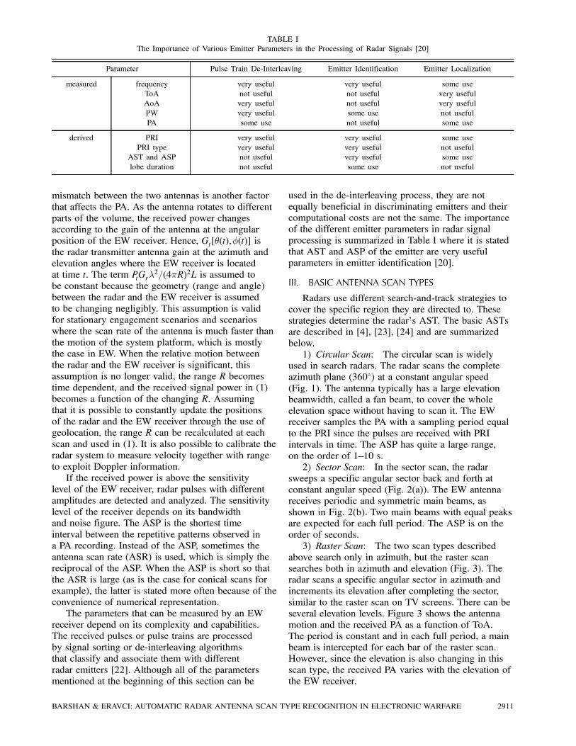
TABLE I

The Importance of Various Emitter Parameters in the Processing of Radar Signals [20]

Parameter Pulse Train De-Interleaving Emitter Identification Emitter Localization

measured frequency very useful very useful some use

ToA not useful not useful very useful

AoA very useful not useful very useful

PW very useful some use not useful

PA some use not useful some use

derived PRI very useful very useful some use

PRI type very useful very useful not useful

AST and ASP not useful very useful some use

lobe duration not useful some use not useful

mismatch between the two antennas is another factor

that affects the PA. As the antenna rotates to different

parts of the volume, the received power changes

according to the gain of the antenna at the angular

position of the EW receiver. Hence, Gt[μ(t),Á(t)] is

the radar transmitter antenna gain at the azimuth and

elevation angles where the EW receiver is located

at time t. The term PtGr¸2=(4¼R)2L is assumed to

be constant because the geometry (range and angle)

between the radar and the EW receiver is assumed

to be changing negligibly. This assumption is valid

for stationary engagement scenarios and scenarios

where the scan rate of the antenna is much faster than

the motion of the system platform, which is mostly

the case in EW. When the relative motion between

the radar and the EW receiver is significant, this

assumption is no longer valid, the range R becomes

time dependent, and the received signal power in (1)

becomes a function of the changing R. Assuming

that it is possible to constantly update the positions

of the radar and the EW receiver through the use of

geolocation, the range R can be recalculated at each

scan and used in (1). It is also possible to calibrate the

radar system to measure velocity together with range

to exploit Doppler information.

If the received power is above the sensitivity

level of the EW receiver, radar pulses with different

amplitudes are detected and analyzed. The sensitivity

level of the receiver depends on its bandwidth

and noise figure. The ASP is the shortest time

interval between the repetitive patterns observed in

a PA recording. Instead of the ASP, sometimes the

antenna scan rate (ASR) is used, which is simply the

reciprocal of the ASP. When the ASP is short so that

the ASR is large (as is the case for conical scans for

example), the latter is stated more often because of the

convenience of numerical representation.

The parameters that can be measured by an EW

receiver depend on its complexity and capabilities.

The received pulses or pulse trains are processed

by signal sorting or de-interleaving algorithms

that classify and associate them with different

radar emitters [22]. Although all of the parameters

mentioned at the beginning of this section can be

used in the de-interleaving process, they are not

equally beneficial in discriminating emitters and their

computational costs are not the same. The importance

of the different emitter parameters in radar signal

processing is summarized in Table I where it is stated

that AST and ASP of the emitter are very useful

parameters in emitter identification [20].

III. BASIC ANTENNA SCAN TYPES

Radars use different search-and-track strategies to

cover the specific region they are directed to. These

strategies determine the radar’s AST. The basic ASTs

are described in [4], [23], [24] and are summarized

below.

1) Circular Scan: The circular scan is widely

used in search radars. The radar scans the complete

azimuth plane (360±) at a constant angular speed(Fig. 1). The antenna typically has a large elevation

beamwidth, called a fan beam, to cover the whole

elevation space without having to scan it. The EW

receiver samples the PA with a sampling period equal

to the PRI since the pulses are received with PRI

intervals in time. The ASP has quite a large range,

on the order of 1—10 s.

2) Sector Scan: In the sector scan, the radar

sweeps a specific angular sector back and forth at

constant angular speed (Fig. 2(a)). The EW antenna

receives periodic and symmetric main beams, as

shown in Fig. 2(b). Two main beams with equal peaks

are expected for each full period. The ASP is on the

order of seconds.

3) Raster Scan: The two scan types described

above search only in azimuth, but the raster scan

searches both in azimuth and elevation (Fig. 3). The

radar scans a specific angular sector in azimuth and

increments its elevation after completing the sector,

similar to the raster scan on TV screens. There can be

several elevation levels. Figure 3 shows the antenna

motion and the received PA as a function of ToA.

The period is constant and in each full period, a main

beam is intercepted for each bar of the raster scan.

However, since the elevation is also changing in this

scan type, the received PA varies with the elevation of

the EW receiver.


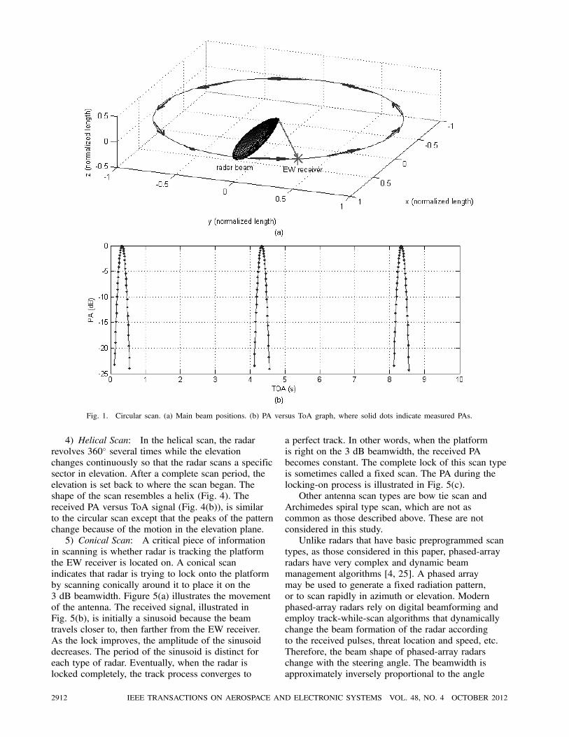
Fig. 1. Circular scan. (a) Main beam positions. (b) PA versus ToA graph, where solid dots indicate measured PAs.

4) Helical Scan: In the helical scan, the radar

revolves 360± several times while the elevationchanges continuously so that the radar scans a specific

sector in elevation. After a complete scan period, the

elevation is set back to where the scan began. The

shape of the scan resembles a helix (Fig. 4). The

received PA versus ToA signal (Fig. 4(b)), is similar

to the circular scan except that the peaks of the pattern

change because of the motion in the elevation plane.

5) Conical Scan: A critical piece of information

in scanning is whether radar is tracking the platform

the EW receiver is located on. A conical scan

indicates that radar is trying to lock onto the platform

by scanning conically around it to place it on the

3 dB beamwidth. Figure 5(a) illustrates the movement

of the antenna. The received signal, illustrated in

Fig. 5(b), is initially a sinusoid because the beam

travels closer to, then farther from the EW receiver.

As the lock improves, the amplitude of the sinusoid

decreases. The period of the sinusoid is distinct for

each type of radar. Eventually, when the radar is

locked completely, the track process converges to

a perfect track. In other words, when the platform

is right on the 3 dB beamwidth, the received PA

becomes constant. The complete lock of this scan type

is sometimes called a fixed scan. The PA during the

locking-on process is illustrated in Fig. 5(c).

Other antenna scan types are bow tie scan and

Archimedes spiral type scan, which are not as

common as those described above. These are not

considered in this study.

Unlike radars that have basic preprogrammed scan

types, as those considered in this paper, phased-array

radars have very complex and dynamic beam

management algorithms [4, 25]. A phased array

may be used to generate a fixed radiation pattern,

or to scan rapidly in azimuth or elevation. Modern

phased-array radars rely on digital beamforming and

employ track-while-scan algorithms that dynamically

change the beam formation of the radar according

to the received pulses, threat location and speed, etc.

Therefore, the beam shape of phased-array radars

change with the steering angle. The beamwidth is

approximately inversely proportional to the angle


Fig. 2. Sector scan. (a) Main beam positions. (b) PA versus ToA graph.

measured from the normal to the antenna [18]. In

addition to the changing shape of the main beam,

the sidelobes also change in appearance and position.

Consequently, the antenna scan pattern received at the

EW receiver keeps changing, complicating the ASP

estimation and AST recognition problem. Instead of

ASP and AST, one can use lobe duration (illumination

time) as a distinctive feature of phased-array radars.

However, one should consider that the lobe duration

may also vary (probably small variations) because of

the beam broadening nature of phased arrays when

looking off the boresight of the array.

IV. ANTENNA SCAN PATTERN SIMULATOR

Because of the scarcity of recorded EW receiver

data, an antenna scan pattern simulator (ASPS) with

a graphical user interface (GUI) is developed using

MATLAB [26]. An example screen of the ASPS is

illustrated in Fig. 6 where the different parts of the

GUI can be seen on the left, and a sample PA versus

ToA plot is shown on the right.

The transmitter antenna of the radar is modeled

as a linear antenna array, with optional weightings

(uniform, triangle, Hamming, Taylor, Poussin, and

Blackman) that determine the sidelobe level of the

antenna pattern. The simulator calculates the number

of elements needed to achieve the desired azimuth

and elevation beamwidths for a particular model and

synthesizes a pattern for them.

The ASTs described in Section III are simulated

by the ASPS. According to the AST selected by

the user, different edit boxes are enabled with

corresponding parameter names. The user inputs the

desired parameters for the particular scan type. Period

is the common parameter for all of the ASTs. Sector

scan requires the start-finish positions in the azimuth

and the elevation position of the beam. Raster scan

acquires the start-finish positions in azimuth and

elevation with the number of bars in the elevation.

Conical scan type needs the target azimuth and

elevation position and squint angle of the radar. All

of the above parameters are used to calculate the beam

position at a specific point in time corresponding to


Fig. 3. Raster scan. (a) Main beam positions. (b) PA versus ToA graph.

the ToA of the pulse. The user can input the ToAs of

the radar pulses that determine the sampling points of

the antenna scan pattern.

As the radar antenna rotates, the gain observed

by the EW receiver (that is the Gt(μ(t),Á(t)) factor

in the received power in (1)) changes with time.

The simulator calculates the beam positions for each

pulse according to the selected AST and ASP. The

properties and the position of the EW receiver with

respect to the radar are given as input. The simulator

then calculates the gain observed at the EW receiver

using the receiver’s azimuthal and elevational position

with respect to the radar. The radar is assumed to

be at the origin of the coordinate system. Then,

the received power at the EW receiver is calculated

for each pulse of the radar using its ToA and the

beam’s position using (1). PAs are normalized so that

the pulse with the maximum power corresponds to

0 dB.

The EW receiver antenna is modeled as isotropic

(i.e., constant Gr) and the propagation loss is assumed

to be constant. It is assumed that the EW receiver

remains stationary (or moves a negligible amount

compared with the radar) so that the range R is

approximately constant throughout the simulation

time. The noise level in the EW receiver is simulated

by the addition of zero-mean Gaussian noise with

the desired power to the signal. The sensitivity level

of the receiver can be adjusted as well. Signals with

amplitudes below the sensitivity level of the receiver

are not detected.

Unmodulated pulses as well as pulses with both

intrapulse and interpulse modulation have been

implemented. The resulting PA versus ToA graphs of

the simulated scenarios can be plotted and explored.

An example is provided in Fig. 6.

The simulator also illustrates how the beam scans

the volume in time. It divides the whole simulation

time into 10 intervals and illustrates the beam position

at these time points and also plots the position of the

EW receiver to see the effects of the rotation of the

beam.


Fig. 4. Helical scan. (a) Main beam positions. (b) PA versus ToA graph.

V. AST RECOGNITION ALGORITHM

The AST recognition problem can be summarized

as estimating the relative angular position of the

EW receiver with respect to the radar main beam as

time passes, and classifying the radar AST into one

of the most frequently encountered scan patterns.

Although it should be possible to infer the AST

based on the power received from the radar, the

problem is complicated in multiple ways: the location

of the radar antenna and its radiation pattern are

completely unknown to the EW receiver, and the

parameters of the ASTs vary vastly (ASP, number

of bars in raster, sector width, etc.). Trying to check

all possible received power outcomes and defining

a metric (e.g., Euclidean distance) to measure the

similarities would exhaust any computation power

feasible. This deficiency of vital information has led

the study to suboptimal solutions, in which several

characteristic features of the radar signal are used.

An overview of the proposed algorithm is given in

Fig. 7.

A. The Input Signal

The input PA versus the ToA data is either the

output of the ASPS or is real data acquired by the

EW receiver. Figure 8(a) shows an example PA versus

a ToA signal from a raster scan where three periods

are shown. Since the output from these sources

are in dBW (decibel relative to Watt), the signal is

first transformed from dBW to Volt (V) scale using

10(power=20).

Although uniform sampling is employed in many

applications, in some cases, nonuniformly sampled

signals can be encountered. Estimating the period of a

uniformly sampled signal is much simpler and usually

independent from the method used. If the signal is

nonuniformly sampled, it is better to resample it

uniformly. For example, signals with stagger-type

PRI result in nonuniform sampling. If this is the case,

the signal is resampled with the highest PRI in the

stagger levels. During the resampling process, if the

signal value is not available at a particular instant,

interpolation is performed using the two nearest


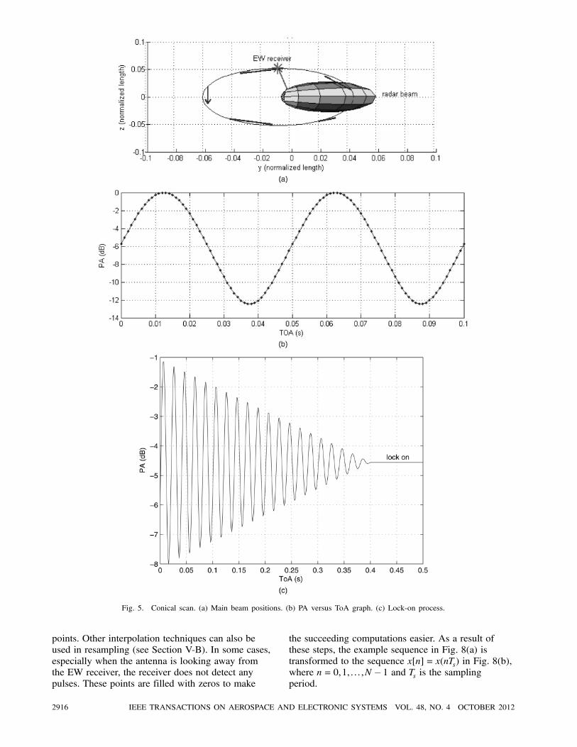
Fig. 5. Conical scan. (a) Main beam positions. (b) PA versus ToA graph. (c) Lock-on process.

points. Other interpolation techniques can also be

used in resampling (see Section V-B). In some cases,

especially when the antenna is looking away from

the EW receiver, the receiver does not detect any

pulses. These points are filled with zeros to make

the succeeding computations easier. As a result of

these steps, the example sequence in Fig. 8(a) is

transformed to the sequence x[n] = x(nTs) in Fig. 8(b),

where n= 0,1, : : : ,N ¡ 1 and Ts is the samplingperiod.


Fig. 6. ASPS GUI: Different parts of GUI can be seen on left, and sample PA versus ToA plot is shown on right.

The input signals are synthesized by using the

ASPS described in the previous section. Parameters of

the synthesized signals (e.g., the PRI, ASP, azimuth

and elevation beamwidths of the radar antenna,

number of bars in raster, sector width) are selected

realistically over a wide range, taking real radar

systems as examples. We used a classified database

for this purpose.

B. Period Estimation

A continuous-time signal x(t) is called periodic

if x(t) = x(t+T) 8t and some period value T. Thesmallest value of T that satisfies this equality is

called the fundamental period. Period estimation

has attracted considerable interest over the years,

especially in the speech processing area [27—31].

The problem is sometimes called (fundamental) tone

estimation or pitch estimation. There are solutions to

the problem in the time and the frequency domains.

Frequency-domain methods estimate the period by

detecting the peaks of the frequency spectrum. This

approach possesses some problems when the signal

is not a sinusoid, but has a wide bandwidth. In this

case, the peaks may be illusive when estimating the

fundamental frequency.

Time-domain methods are particularly useful for

period estimation of nonsinusoidal signals. These

methods define some kind of similarity metric and try

to maximize the similarity with the lagged versions

of the signal using this metric. For example, the

average magnitude difference or the autocorrelation

between the signal and its lagged versions can be

used as similarity metrics. The lag value where the

similarity is maximized corresponds to the period

estimate of the signal. The latter approach provides

the best performance when the noise for each of the

two signals is white Gaussian noise (which usually is

the case).

The backbone of our algorithm is the ASP

estimation, which affects the overall performance of

AST classification significantly. An ASP has a very

large range whose true value is usually acquired from

intelligence agencies. The ASP estimation method

should be chosen according to the properties of the

signal. In this study period estimation is performed by

using the normalized autocorrelation coefficients of


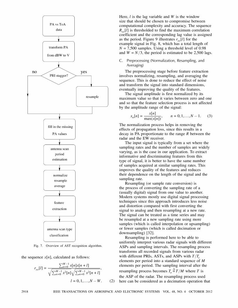
Fig. 7. Overview of AST recognition algorithm.

the sequence x[n], calculated as follows:

rxx[l] =

PW¡1n=0 x[n]x[n+ l]qPW¡1

n=0 x2[n]

qPW¡1n=0 x

2[n+ l]

,

l = 0,1, : : : ,N ¡W: (2)

Here, l is the lag variable and W is the windowsize that should be chosen to compromise betweencomputational complexity and accuracy. The sequenceRxx[l] is thresholded to find the maximum correlationcoefficient and the corresponding lag value is assignedas the period. Figure 9 illustrates rxx[l] for theexample signal in Fig. 8, which has a total length ofN = 7,500 samples. Using a threshold level of 0.98and W =N=3, the period is estimated to be 2,500 lags.

C. Preprocessing (Normalization, Resampling, andAveraging)

The preprocessing stage before feature extractioninvolves normalizing, resampling, and averaging thesequence. This is done to reduce the effect of noiseand transform the signal into standard dimensions,eventually improving the quality of the features.The signal amplitude is first normalized by its

maximum value so that it varies between zero and oneand so that the feature selection process is not affectedby the amplitude range of the signal:

xn[n] =x[n]

max(x[n]), n= 0,1, : : : ,N ¡ 1: (3)

The normalization process helps in removing theeffects of propagation loss, since this results in adecay in PA proportionate to the range R between theradar and the EW receiver.The input signal is typically from a set where the

sampling rates and the number of samples are widelyvarying, as is the case in our application. To extractinformative and discriminating features from thistype of signal, it is better to have the same numberof samples acquired at similar sampling rates. Thisimproves the quality of the features and reducestheir dependence on the length of the signal and thesampling rate.Resampling (or sample rate conversion) is

the process of converting the sampling rate of a(usually digital) signal from one value to another.Modern systems mostly use digital signal processingtechniques since this approach introduces less noiseand distortion compared with first converting thesignal to analog and then resampling at a new rate.The signal can be treated as a time series and maybe resampled at a new sampling rate using moresamples (which is called interpolation or upsampling)or fewer samples (which is called decimation ordownsampling) [32].

Resampling is performed here to be able to

uniformly interpret various radar signals with different

ASPs and sampling intervals. The resampling process

transforms all recorded signals from various radar

with different PRIs, ASTs, and ASPs with T=Tselements per period into a standard sequence of M

elements per period. The sampling interval after the

resampling process becomes To¢=T=M where T is

the ASP of the radar. The resampling process used

here can be considered as a decimation operation that


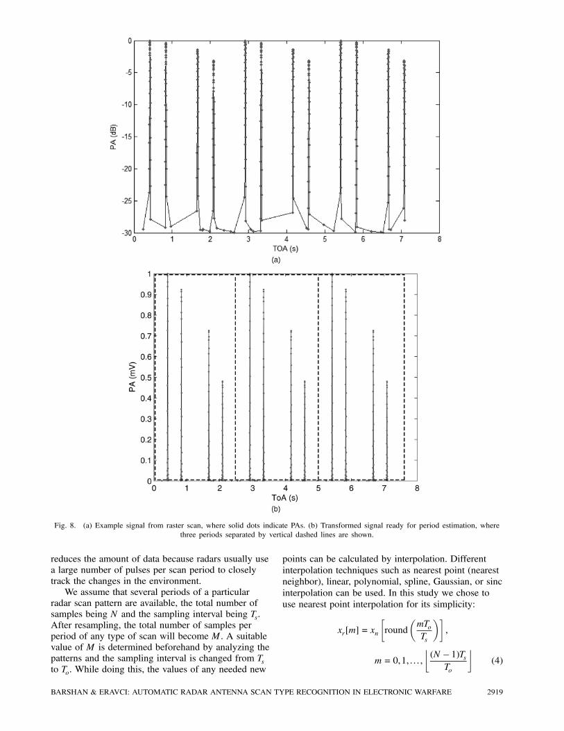
Fig. 8. (a) Example signal from raster scan, where solid dots indicate PAs. (b) Transformed signal ready for period estimation, where

three periods separated by vertical dashed lines are shown.

reduces the amount of data because radars usually use

a large number of pulses per scan period to closely

track the changes in the environment.

We assume that several periods of a particular

radar scan pattern are available, the total number of

samples being N and the sampling interval being Ts.

After resampling, the total number of samples per

period of any type of scan will become M. A suitable

value of M is determined beforehand by analyzing the

patterns and the sampling interval is changed from Tsto To. While doing this, the values of any needed new

points can be calculated by interpolation. Different

interpolation techniques such as nearest point (nearest

neighbor), linear, polynomial, spline, Gaussian, or sinc

interpolation can be used. In this study we chose to

use nearest point interpolation for its simplicity:

xr[m] = xn

·round

μmToTs

¶¸,

m= 0,1, : : : ,

¹(N ¡ 1)Ts

To

º(4)


Fig. 9. Normalized autocorrelation coefficients of example sequence.

where xr[m] denotes the resampled sequence and b:cindicates truncation. The nearest point interpolation

rounds off noninteger mTo=Ts values to the nearest

integer so that the resampled sequence at a specific

point m takes the value of its nearest neighbor in

the normalized sequence. The values of the other

neighboring points are not considered. This type of

interpolation has the advantage of being simple and

fast. Because a high sampling rate is available before

the resampling process, the nearest point interpolation

technique results in negligible distortion in the signal.

It is assumed that the input signal has at least two

cycles of the antenna scan. This is important because

the period estimation phase needs at least a few cycles

to reduce the effect of noise and to accurately estimate

the signal period. If at least K complete periods are

available for period estimation so that NTs ¸KT, thesecan be coherently averaged as

x[m] =1

K

K¡1Xk=0

xr[m+ kM], m= 0,1, : : : ,M ¡ 1:

(5)The example sequence after normalization,

resampling, and averaging over three periods is

depicted in Fig. 10 where an M value of 2,000 is

used. From this point on in the text, the word “signal”

refers to this averaged sequence.

D. Feature Extraction

Input to the feature extraction part is the

preprocessed sequence with M elements and sampling

interval To. A total of 100 data sequences is generated

by the ASPS, 20 from each of the following ASTs

in the given order: circular, sector, raster, helical, and

conical. While generating the simulated training data,

we have varied a number of different parameters so

that the training samples resemble the real data from

different realistic scenarios as much as possible. For

the four ASTs other than the conical, the ASP is

uniformly varied between 1—10 s (ASR: 0.1—1 Hz).

For the conical scan (whose scan rate is much faster

compared with the other scans), the ASP is uniformly

varied between 0.01—0.2 s (ASR: 5—100 Hz) in

generating the 20 training data samples.

The azimuth and elevation sector widths, EW

position with respect to the radar, and the squint angle

related to the radar-EW receiver engagement have also

been varied. For the circular antenna scan pattern, the

azimuth angle has a uniform random distribution in

[0,360±]. For the sector scan, different sector widthsin [0,180±] are used and the position of the EWreceiver within the sector is randomly selected with

uniform distribution. For the raster scan, the azimuth

is varied in [0,180±], whereas for the helical scan, thecorresponding interval is [0,360±]. In the latter twoASTs, the elevation is varied in [0,10±] and again, theposition of the EW receiver is randomly selected. For

the conical scan, random locations around the position

tracked by the radar are used for the EW receiver.

Features such as the minimum and the maximum

values, mean, standard deviation, skewness, kurtosis,

or higher order moments are commonly employed

to describe the probability density function of the

signal. Coefficients of various transforms such as FFT,


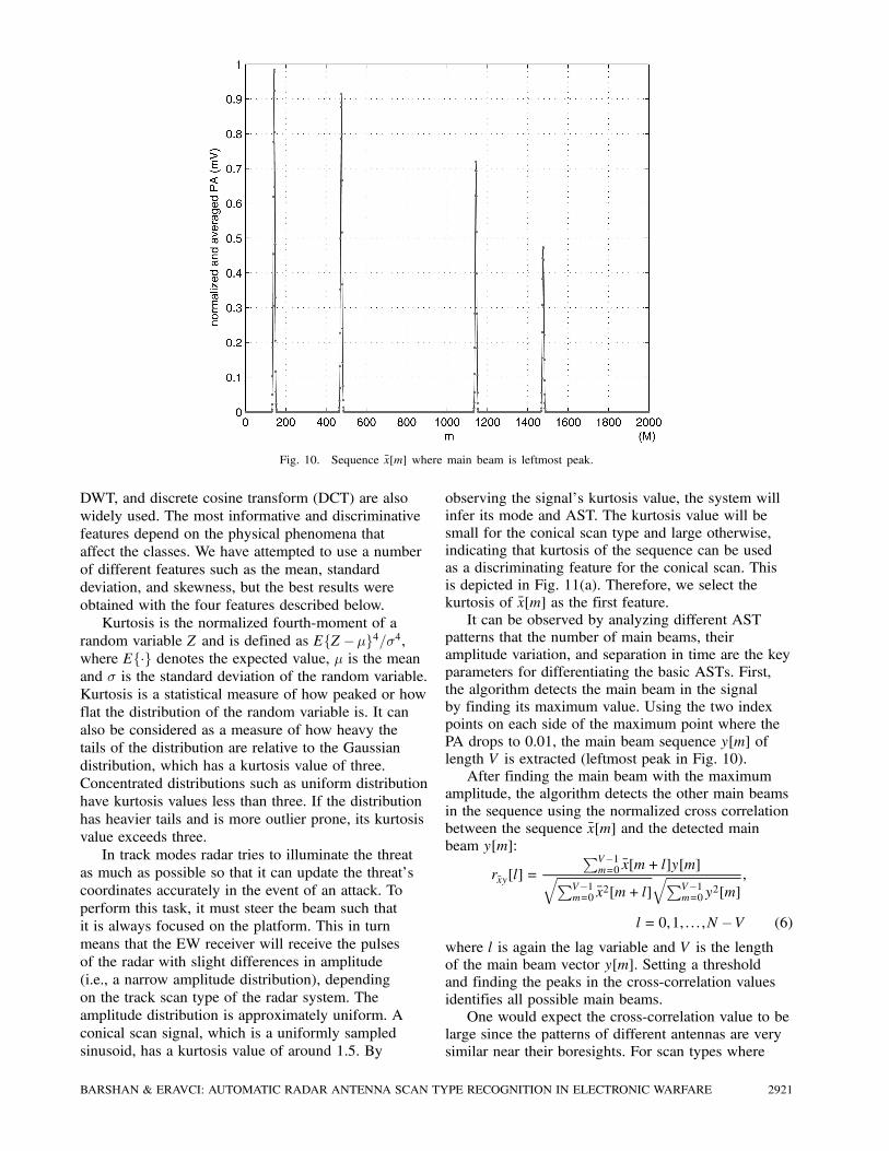
Fig. 10. Sequence x[m] where main beam is leftmost peak.

DWT, and discrete cosine transform (DCT) are also

widely used. The most informative and discriminative

features depend on the physical phenomena that

affect the classes. We have attempted to use a number

of different features such as the mean, standard

deviation, and skewness, but the best results were

obtained with the four features described below.

Kurtosis is the normalized fourth-moment of a

random variable Z and is defined as EfZ ¡¹g4=¾4,where Ef¢g denotes the expected value, ¹ is the meanand ¾ is the standard deviation of the random variable.

Kurtosis is a statistical measure of how peaked or how

flat the distribution of the random variable is. It can

also be considered as a measure of how heavy the

tails of the distribution are relative to the Gaussian

distribution, which has a kurtosis value of three.

Concentrated distributions such as uniform distribution

have kurtosis values less than three. If the distribution

has heavier tails and is more outlier prone, its kurtosis

value exceeds three.

In track modes radar tries to illuminate the threat

as much as possible so that it can update the threat’s

coordinates accurately in the event of an attack. To

perform this task, it must steer the beam such that

it is always focused on the platform. This in turn

means that the EW receiver will receive the pulses

of the radar with slight differences in amplitude

(i.e., a narrow amplitude distribution), depending

on the track scan type of the radar system. The

amplitude distribution is approximately uniform. A

conical scan signal, which is a uniformly sampled

sinusoid, has a kurtosis value of around 1.5. By

observing the signal’s kurtosis value, the system will

infer its mode and AST. The kurtosis value will be

small for the conical scan type and large otherwise,

indicating that kurtosis of the sequence can be used

as a discriminating feature for the conical scan. This

is depicted in Fig. 11(a). Therefore, we select the

kurtosis of x[m] as the first feature.

It can be observed by analyzing different AST

patterns that the number of main beams, their

amplitude variation, and separation in time are the key

parameters for differentiating the basic ASTs. First,

the algorithm detects the main beam in the signal

by finding its maximum value. Using the two index

points on each side of the maximum point where the

PA drops to 0.01, the main beam sequence y[m] of

length V is extracted (leftmost peak in Fig. 10).

After finding the main beam with the maximum

amplitude, the algorithm detects the other main beams

in the sequence using the normalized cross correlation

between the sequence x[m] and the detected main

beam y[m]:

rxy[l] =

PV¡1m=0 x[m+ l]y[m]qPV¡1

m=0 x2[m+ l]

qPV¡1m=0 y

2[m]

,

l = 0,1, : : : ,N ¡V (6)

where l is again the lag variable and V is the length

of the main beam vector y[m]. Setting a threshold

and finding the peaks in the cross-correlation values

identifies all possible main beams.

One would expect the cross-correlation value to be

large since the patterns of different antennas are very

similar near their boresights. For scan types where


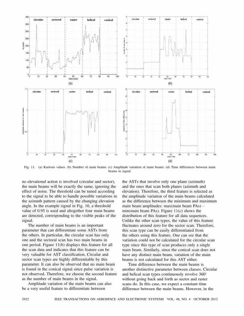
Fig. 11. (a) Kurtosis values. (b) Number of main beams. (c) Amplitude variation of main beams. (d) Time differences between main

beams in signal.

no elevational action is involved (circular and sector),

the main beams will be exactly the same, ignoring the

effect of noise. The threshold can be tuned according

to the signal to be able to handle possible variations in

the azimuth pattern caused by the changing elevation

angle. In the example signal in Fig. 10, a threshold

value of 0.95 is used and altogether four main beams

are detected, corresponding to the visible peaks of the

signal.

The number of main beams is an important

parameter that can differentiate some ASTs from

the others. In particular, the circular scan has only

one and the sectoral scan has two main beams in

one period. Figure 11(b) displays this feature for all

the scan data and indicates that this feature can be

very valuable for AST classification. Circular and

sector scan types are highly differentiable by this

parameter. It can also be observed that no main beam

is found in the conical signal since pulse variation is

not observed. Therefore, we choose the second feature

as the number of main beams in the signal.

Amplitude variation of the main beams can also

be a very useful feature to differentiate between

the ASTs that involve only one plane (azimuth)

and the ones that scan both planes (azimuth and

elevation). Therefore, the third feature is selected as

the amplitude variation of the main beams calculated

as the difference between the minimum and maximum

main beam amplitudes: max(main beam PAs)¡min(main beam PAs). Figure 11(c) shows the

distribution of this feature for all data sequences.

Unlike the other scan types, the value of this feature

fluctuates around zero for the sector scan. Therefore,

this scan type can be easily differentiated from

the others using this feature. One can see that the

variation could not be calculated for the circular scan

type since this type of scan produces only a single

main beam. Similarly, since the conical scan does not

have any distinct main beam, variation of the main

beams is not calculated for this AST either.

Time difference between the main beams is

another distinctive parameter between classes. Circular

and helical scan types continuously revolve 360±

without going back and forth as sector and raster

scans do. In this case, we expect a constant time

difference between the main beams. However, in the


raster scan, the time difference between the main

beams usually varies because of the nature of the

scan. The only case where the time difference will be

the same is when the EW receiver is in the middle of

the scanned sector, and this is unlikely. Therefore, the

ratio of the maximum of the time differences to the

minimum is calculated and used as the fourth feature.

Note that this feature is only calculable for helical and

raster scans since there should be at least three main

beams to calculate the variation of time differences

between the main beams (Fig. 11(d)). For features that

cannot be calculated for some of the ASTs, a value

of 10,000 is used as an indicator to the classification

stage.

E. Classification

We associate a class ci with each AST (i=

1, : : : ,Nc). An unknown AST is assigned to class

ci if its feature vector z= [z1, : : : ,zNF ]T falls in the

region −i. A rule that partitions the decision space into

regions −i, i= 1, : : : ,Nc is called a decision rule. Each

one of these regions corresponds to a different AST.

Boundaries between these regions are called decision

surfaces.

The training set, which consists of a total of Npsample feature vectors, is used to develop the decision

rule or to train the classifier. The test set is then used

to evaluate the performance of the classifier.

The four selected features are used in the

classification process with the naive Bayes (NB),

decision tree (DT), ANN, and support vector machine

(SVM) classifiers [33]:

1) Naive Bayes Classifier: In classification

problems, when there are more than a few features

and classes, usually a large number of observations

is needed to estimate the probabilities of a pattern

belonging to different classes. The NB classifier

is a simple probabilistic classifier that gets around

this problem by not requiring a large number of

observations for each possible combination of

the features [34]. It is one of the most efficient

and effective inductive learning algorithms for

machine learning and data mining that is particularly

suitable when the dimensionality of the features

is high. Parameters of the probabilistic model are

calculated under the assumption that the features

are independent of each other. In other words, an

NB classifier assumes that the presence (or absence)

of a particular feature of a class is unrelated to the

presence (or absence) of any other feature. The

features independently contribute to the probability of

a pattern belonging to different classes. Although this

assumption is rarely true in real-world applications, it

is made to simplify the computations and in this sense

considered to be naive.

NB classifiers can be trained very efficiently with

fewer observations in a supervised learning setting.

Despite their naive design, simplicity, and apparently

oversimplified assumptions, these classifiers work

surprisingly well in many complex real-world

situations and can often outperform more sophisticated

classification methods.

Given the classes c1,c2, : : : ,cNc , let p(ci) be the a

priori probability of an AST belonging to class ci. To

classify an AST with feature vector z, a posterioriprobabilities p(ci j z) are compared and the scanpattern is classified into class cj if p(cj j z)> p(ci j z)8i 6= j. This is known as Bayes minimum error rule.

However, since these a posteriori probabilities are

rarely known, they need to be estimated. A more

convenient formulation of this rule can be obtained

by using Bayes’ theorem: p(ci j z) = p(z j ci)p(ci)=p(z),where p(z) =

PNci=1p(z j ci)p(ci) is the total probability.

This results in p(z j cj)p(cj)> p(z j ci)p(ci) 8i 6= j) z 2−j where p(z j ci) are the class-conditionalprobability density functions that are also unknown

and need to be estimated in their turn based on the

training set. Probabilistic models for p(z j ci) aredeveloped first, using the available training data for

each class. As mentioned above, a major advantage

of the NB classifier is that it requires only a small

amount of training data to estimate the parameters

(means and variances of the features) necessary

for classification. Since features are assumed to be

independent, it is not necessary to estimate the entire

covariance matrix; only the variances of the features

for each class need to be determined. NB can be

modeled in several different ways including normal,

lognormal, gamma, and Poisson density functions.

In this study, the probability density functions are

modeled as normal distributions whose parameters

(mean and variance) are calculated by maximum

likelihood estimation. Then, the posterior probabilities

are calculated according to the probabilistic models

of each class by applying the Bayes’ theorem given

above. The class of the signal is chosen as the one

with the highest posterior probability according to

Bayes minimum error rule. Thus, the decision rule

for classification is merely picking the hypothesis

that is the most probable. This decision rule can be

generalized as qj(z)> qi(z) 8i 6= j) z 2 −j where the

function qi is called a discriminant function.

2) Decision-Tree Classifier: DT classifiers are one

of the most intuitive and natural classifiers and are

fast, comprehensible, and easy to visualize [33]. A DT

can be considered as a sequential procedure to classify

given input patterns. It follows predefined rules or test

conditions at each node of the tree and makes binary

decisions based on these conditions. Rules correspond

to conditions such as “is feature zi · ¿i?,” where ¿is the threshold value for a given feature and i=

1,2, : : : ,NF , with NF being the total number of features

used [34]. Features should be selected and calculated

before using them in the DT to make the algorithm

independent of the calculation cost of different


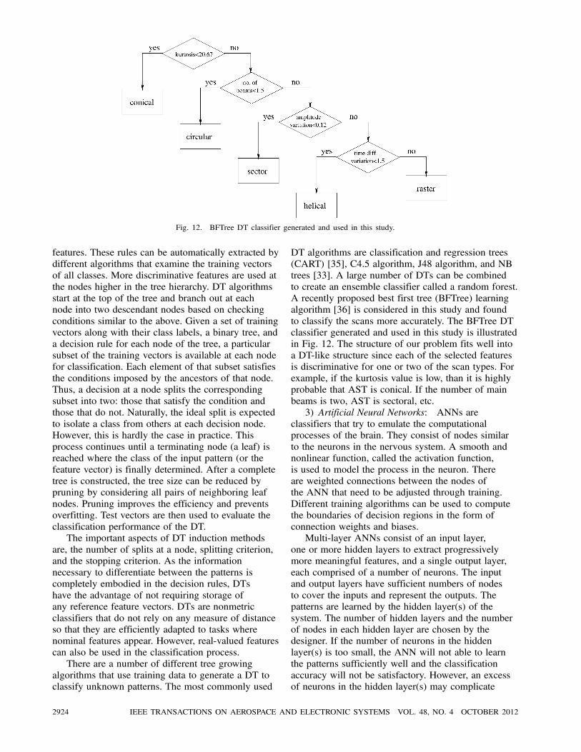
Fig. 12. BFTree DT classifier generated and used in this study.

features. These rules can be automatically extracted by

different algorithms that examine the training vectors

of all classes. More discriminative features are used at

the nodes higher in the tree hierarchy. DT algorithms

start at the top of the tree and branch out at each

node into two descendant nodes based on checking

conditions similar to the above. Given a set of training

vectors along with their class labels, a binary tree, and

a decision rule for each node of the tree, a particular

subset of the training vectors is available at each node

for classification. Each element of that subset satisfies

the conditions imposed by the ancestors of that node.

Thus, a decision at a node splits the corresponding

subset into two: those that satisfy the condition and

those that do not. Naturally, the ideal split is expected

to isolate a class from others at each decision node.

However, this is hardly the case in practice. This

process continues until a terminating node (a leaf) is

reached where the class of the input pattern (or the

feature vector) is finally determined. After a complete

tree is constructed, the tree size can be reduced by

pruning by considering all pairs of neighboring leaf

nodes. Pruning improves the efficiency and prevents

overfitting. Test vectors are then used to evaluate the

classification performance of the DT.

The important aspects of DT induction methods

are, the number of splits at a node, splitting criterion,

and the stopping criterion. As the information

necessary to differentiate between the patterns is

completely embodied in the decision rules, DTs

have the advantage of not requiring storage of

any reference feature vectors. DTs are nonmetric

classifiers that do not rely on any measure of distance

so that they are efficiently adapted to tasks where

nominal features appear. However, real-valued features

can also be used in the classification process.

There are a number of different tree growing

algorithms that use training data to generate a DT to

classify unknown patterns. The most commonly used

DT algorithms are classification and regression trees

(CART) [35], C4.5 algorithm, J48 algorithm, and NB

trees [33]. A large number of DTs can be combined

to create an ensemble classifier called a random forest.

A recently proposed best first tree (BFTree) learning

algorithm [36] is considered in this study and found

to classify the scans more accurately. The BFTree DT

classifier generated and used in this study is illustrated

in Fig. 12. The structure of our problem fits well into

a DT-like structure since each of the selected features

is discriminative for one or two of the scan types. For

example, if the kurtosis value is low, than it is highly

probable that AST is conical. If the number of main

beams is two, AST is sectoral, etc.

3) Artificial Neural Networks: ANNs are

classifiers that try to emulate the computational

processes of the brain. They consist of nodes similar

to the neurons in the nervous system. A smooth and

nonlinear function, called the activation function,

is used to model the process in the neuron. There

are weighted connections between the nodes of

the ANN that need to be adjusted through training.

Different training algorithms can be used to compute

the boundaries of decision regions in the form of

connection weights and biases.

Multi-layer ANNs consist of an input layer,

one or more hidden layers to extract progressively

more meaningful features, and a single output layer,

each comprised of a number of neurons. The input

and output layers have sufficient numbers of nodes

to cover the inputs and represent the outputs. The

patterns are learned by the hidden layer(s) of the

system. The number of hidden layers and the number

of nodes in each hidden layer are chosen by the

designer. If the number of neurons in the hidden

layer(s) is too small, the ANN will not able to learn

the patterns sufficiently well and the classification

accuracy will not be satisfactory. However, an excess

of neurons in the hidden layer(s) may complicate


the training process and may lead to memorizing

the signal instead of learning its dynamics. Due to

the presence of distributed nonlinearity and a high

degree of connectivity, theoretical analysis of ANNs is

difficult. The performance of ANNs is affected by the

choice of parameters related to the network structure,

training algorithm, and input signals, as well as by

parameter initialization [37].

There is a variety of network architectures, training

algorithms, and activation functions for different

applications [37]. In this study, the back-propagation

algorithm [37] is used for training, by presenting a set

of training patterns to the network. Back propagation

is a supervised method that uses a gradient-descent

procedure based on the error at the output. It tries to

minimize the error by feeding the error at the output

back to update the weights in each epoch. Different

initial conditions and different numbers of neurons

in the hidden layer have been considered. The aim is

to minimize the average of the sum of squared errors

over all training vectors:

Eav(w) =1

2Np

NpXi=1

NcXj=1

[dij ¡ oij(w)]2: (7)

Here, w is the weight vector, dij and oij are thedesired and actual output values for the ith training

pattern and the jth output neuron, and Np is the total

number of training patterns. When the entire training

set is covered, an epoch is completed. The error

between the desired and actual outputs is computed at

the end of each iteration and these errors are averaged

at the end of each epoch (see (7)). The training

process is terminated when a certain precision goal

on the average error is reached or if the specified

maximum number of epochs (5,000) is exceeded,

whichever occurs earlier. The latter case occurs very

rarely. The acceptable average error level is set to a

value of 5%. The weights are initialized randomly

with a uniform distribution in the interval [0,1], and

the learning rate is chosen as 0.05.

After the network is trained, classification is

performed. In the test phase, the test feature vectors

are fed forward to the ANN, with the already

converged weights, and the class of the signal is

determined according to the output. The output

neurons can take continuous values between 0 and 1.

The outputs are compared with the desired outputs,

and the error between them is calculated. The test

vector is said to be correctly classified if this error

is below a threshold value of 0.15.

In this work a fully connected three-layer ANN

is used for classifying radar scan patterns. The input

layer has as many neurons as the number of features

used (or NF , the dimension of the feature vectors),

which is four here. The hidden layer has 10 neurons,

and the output layer has five neurons, equal to the

number of classes Nc. In the input and hidden layers

each, there is an additional neuron with a bias value

of one. For an input feature vector z 2 <4, the desiredoutput is one for the class that the vector belongs to,

and zero for all other output neurons. The sigmoid

function used as the activation function in the hidden

and output layers is given by g(x) = (1+ e¡x)¡1.4) Support Vector Machines: SVMs are binary

classifiers that try to partition the feature space with

hyperplanes where each separated volume represents

a different class [38]. This machine learning technique

was first proposed early in the 1980s [39]. It has

been used in applications such as object, voice,

and handwritten character recognition, and text

classification.

Consider a binary classification problem where

Np training feature vectors zi in some vector space Zand their binary class labels ì 2 f¡1,1g are available,where ì = `(zi) and i = 1, : : : ,Np. The goal in trainingan SVM is to find the hyperplane that maximizes the

margin of separation between the classes so that the

generalization of the classifier is better. All vectors

lying on one side of the hyperplane (class 1) are

labeled as ì =+1, and all vectors lying on the other

side (class 2) are labeled as ì =¡1. The supportvectors are the training patterns that lie closest to the

hyperplane and are at equal distance from it. They

define the optimal separating hyperplane and are

the most difficult patterns to classify, yet the most

informative for the classification task.

If the feature vectors in the original feature space

are not linearly separable, SVMs preprocess and

represent them in a space of higher dimensionality

where they become linearly separable. With a

suitable nonlinear mapping '(:) to a sufficiently

high dimension, data from two different classes can

always be made linearly separable, and separated by

a hyperplane. The choice of the nonlinear mapping

depends on the prior information available to the

designer. If such information is not available, one

might choose to use polynomials, Gaussians, or other

types of basis functions. The dimensionality of the

transformed (mapped) space can sometimes be much

higher than the original feature space.

The projection of the original training data in

space Z to a higher dimensional feature space F is

performed by using a Mercer kernel operator or kernel

function K [40]. We consider a set of classifiers ofthe form q(z) =

PNpi=1¯iK(zi,z) where q(z) is a linear

discriminant function in the transformed space. When

q(z)¸ 0, we label z as +1, otherwise as ¡1. WhenK satisfies Mercer’s condition, K(zi,z) = '(zi) ¢'(z)where '(:) : Z !F is a nonlinear mapping mentioned

above and “¢” denotes the inner or dot product of twovectors. We can then rewrite q(z) in the transformed

space as q(z) = a ¢'(z), where a=PNpi=1¯i'(zi)

is a weight vector. The separating hyperplane is

a ¢'(z) = 0. (Here, both the weight vector a and thetransformed feature vector '(zi) have been augmented


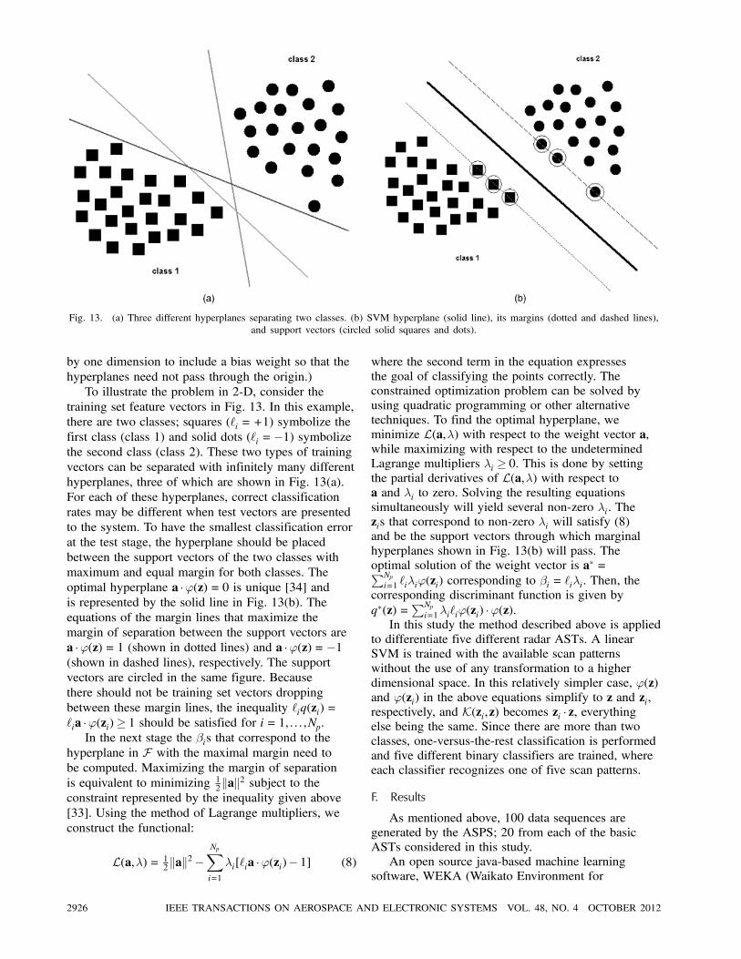
Fig. 13. (a) Three different hyperplanes separating two classes. (b) SVM hyperplane (solid line), its margins (dotted and dashed lines),

and support vectors (circled solid squares and dots).

by one dimension to include a bias weight so that the

hyperplanes need not pass through the origin.)

To illustrate the problem in 2-D, consider the

training set feature vectors in Fig. 13. In this example,

there are two classes; squares (ì =+1) symbolize the

first class (class 1) and solid dots (ì =¡1) symbolizethe second class (class 2). These two types of training

vectors can be separated with infinitely many different

hyperplanes, three of which are shown in Fig. 13(a).

For each of these hyperplanes, correct classification

rates may be different when test vectors are presented

to the system. To have the smallest classification error

at the test stage, the hyperplane should be placed

between the support vectors of the two classes with

maximum and equal margin for both classes. The

optimal hyperplane a ¢'(z) = 0 is unique [34] andis represented by the solid line in Fig. 13(b). The

equations of the margin lines that maximize the

margin of separation between the support vectors are

a ¢'(z) = 1 (shown in dotted lines) and a ¢'(z) =¡1(shown in dashed lines), respectively. The support

vectors are circled in the same figure. Because

there should not be training set vectors dropping

between these margin lines, the inequality ìq(zi) =

ìa ¢'(zi)¸ 1 should be satisfied for i= 1, : : : ,Np.In the next stage the ¯is that correspond to the

hyperplane in F with the maximal margin need to

be computed. Maximizing the margin of separation

is equivalent to minimizing 12kak2 subject to the

constraint represented by the inequality given above

[33]. Using the method of Lagrange multipliers, we

construct the functional:

L(a,¸) = 12kak2¡

NpXi=1

¸i[ìa ¢'(zi)¡ 1] (8)

where the second term in the equation expresses

the goal of classifying the points correctly. The

constrained optimization problem can be solved by

using quadratic programming or other alternative

techniques. To find the optimal hyperplane, we

minimize L(a,¸) with respect to the weight vector a,while maximizing with respect to the undetermined

Lagrange multipliers ¸i ¸ 0. This is done by settingthe partial derivatives of L(a,¸) with respect toa and ¸i to zero. Solving the resulting equations

simultaneously will yield several non-zero ¸i. The

zis that correspond to non-zero ¸i will satisfy (8)

and be the support vectors through which marginal

hyperplanes shown in Fig. 13(b) will pass. The

optimal solution of the weight vector is a¤ =PNpi=1 ì¸i'(zi) corresponding to ¯i = ì¸i. Then, the

corresponding discriminant function is given by

q¤(z) =PNp

i=1¸iì'(zi) ¢'(z).In this study the method described above is applied

to differentiate five different radar ASTs. A linear

SVM is trained with the available scan patterns

without the use of any transformation to a higher

dimensional space. In this relatively simpler case, '(z)

and '(zi) in the above equations simplify to z and zi,

respectively, and K(zi,z) becomes zi ¢ z, everythingelse being the same. Since there are more than two

classes, one-versus-the-rest classification is performed

and five different binary classifiers are trained, where

each classifier recognizes one of five scan patterns.

F. Results

As mentioned above, 100 data sequences are

generated by the ASPS; 20 from each of the basic

ASTs considered in this study.

An open source java-based machine learning

software, WEKA (Waikato Environment for


Fig. 14. Classification results of four classifiers as function of M.

Knowledge Analysis), developed by The University

of Waikato, New Zealand, is used in the classification

process [41]. We have used a four-fold cross-

validation technique for training and testing the

algorithm where the feature vectors from each class

are randomly partitioned into four. In each of the four

runs, one of the partitions is retained for testing and

the remaining three are used for training. This way, all

of the feature vectors are tested [42].

Figure 14 illustrates the classification results with

respect to different M values for all four classifiers

to see the effect of the number of samples per

period. It can be observed that for small values

of M, the signal is undersampled and the features

are not correctly extracted, causing errors in the

classification process. For SVM, the cases where

M < 1,000 did not converge. For M ¸ 1,000, theclassification percentage saturates around 99%. One

can conclude from the figure that M = 1,000 is a good

compromise between the classification accuracy and

computational complexity. The confusion matrices

of the classifiers for M = 1,000 are given in Table II

where the differentiation accuracy is equal or above

97%. The DT classifier results in greater classification

accuracy than the other classifiers.

The effect of noise is also considered and

analyzed. Added noise affects the detected signal

levels because of the thresholding process in the

detection of the pulses. A threshold level 10 dB

TABLE II

Confusion Matrices of the (a) NB, (b) DT, (c) ANN, (d) SVM

Classifiers: 98%, 100%, 97%, and 99% Correct Classification

Rates are Achieved, Respectively

Classified

Circular Sector Raster Helical Conical

(a) true class circular 19 1 0 0 0

sector 1 19 0 0 0

raster 0 0 20 0 0

helical 0 0 0 20 0

conical 0 0 0 0 20

(b) true class circular 20 0 0 0 0

sector 0 20 0 0 0

raster 0 0 20 0 0

helical 0 0 0 20 0

conical 0 0 0 0 20

(c) true class circular 20 0 0 0 0

sector 0 19 1 0 0

raster 0 2 18 0 0

helical 0 0 0 20 0

conical 0 0 0 0 20

(d) true class circular 20 0 0 0 0

sector 0 19 0 1 0

raster 0 0 20 0 0

helical 0 0 0 20 0

conical 0 0 0 0 20

above the noise power level is used in this analysis. A

similar threshold level is usually used in EW systems

as a good compromise between the probability of


Fig. 15. Classification results of four classifiers for different SNRs.

detection and the probability of false alarm [4].

Thresholding limits the range of the PA versus ToA

signal. This, of course, may result in the loss of the

mainlobes, especially in the raster and helical scans,

leading to classification errors. For example, because

of the limited amplitude range of the signal, only one

bar of the raster scan may be observed, which leads to

an erroneous circular scan classification. Classification

results with changing signal-to-noise ratios (SNRs) are

shown in Fig. 15; we used SNR values of 12, 15, 20,

25, 30, 35, and 40 dB. The breakdown in performance

around 25 dB SNR is caused by the limited amplitude

range of the signal, discussed earlier. This limited

range indicates a tendency towards sector and circular

scans both of which are azimuth-only scans and

relatively immune to the range of the received signal.

We have also observed that when the sinusoidal shape

in a conical scan is distorted by the loss of pulses,

the algorithm again has a tendency towards a circular

scan. The results also indicate that ANN is less robust

to noise compared with the other classifiers. The

confusion matrices of all four classifiers for the 20 dB

SNR case are given in Table III.

The analysis has also shown that the noise level

of the EW receiver greatly affects the classification

performance; the signal’s amplitude range decreases

with increasing noise level. The amplitude range of

the signal is very important, especially for ASTs

that scan both in azimuth and elevation (raster and

helical). The range limitation of the signal results in

information loss (main beams with different elevation

TABLE III

Confusion Matrices of the (a) NB, (b) DT, (c) ANN, (d) SVM

classifiers for 20 dB SNR: 77%, 77%, 70%, and 75% Correct

Classification Rates are Achieved, Respectively

Classified

Circular Sector Raster Helical Conical

(a) true class circular 19 1 0 0 0

sector 1 19 0 0 0

raster 6 0 4 10 0

helical 0 5 0 15 0

conical 2 0 0 0 18

(b) true class circular 20 0 0 0 0

sector 1 15 0 4 0

raster 7 0 8 5 0

helical 3 3 0 14 0

conical 0 0 0 0 20

(c) true class circular 20 0 0 0 0

sector 0 18 0 2 0

raster 8 1 6 5 0

helical 3 3 6 8 0

conical 2 0 0 0 18

(d) true class circular 20 0 0 0 0

sector 0 18 0 2 0

raster 7 3 6 4 0

helical 3 4 0 13 0

conical 2 0 0 0 18

levels are not sensed in the EW receiver); it cannot

be inferred in any other way because of the detection

schemes of the EW receivers. The classification

accuracy of raster and helical scans degrades

significantly with the signal’s range limitation.


TABLE IV

Time Needed for Training and Testing Each Classifier

classifier NB DT ANN SVM

time (s) 0.08 0.05 0.35 0.12

Circular, conical, and sector scans are more robust

to this effect. To make the algorithm more reliable,

a simple check of amplitude range can be included

before the algorithm is executed. A range greater than

15 dB (SNR¸ 25 dB) ensures classification accuraciesabove 90%.

1) Comparison of the Computational Time of

the Classifiers: To determine the computational

complexity of the classifiers considered in this study,

we analyzed the time it takes to train and test each

classifier. A computer with a 2.66 GHz processor and

3 GB of RAM was used for this purpose. The results,

obtained with WEKA and given in Table IV, indicate

that the DT classifier outperforms the other classifiers

in this aspect as well.

2) Validation with Real Signals: ASELSAN Inc.

[43] acquired real signals from different pulsed radar

with its own EW receivers configured on a moving

airborne platform. The recorded signals were PRI

modulated but intrapulse modulation was not used.

ASELSAN Inc. provided the data for validation

purposes only; its description and illustration were

strictly forbidden because of the classification level.

Since the EW platform was moving, the assumption

of stationarity of the EW receiver (Section II) was

not met, making the classification process even more

challenging. The signal also had some outliers caused

by the movement of and reflections from the platform.

These effects resulted in distortions in the main beam.

The algorithm had to be modified because of

the properties of the signal. The threshold level in

period estimation was decreased to 0.85 because of

the effect of non-Gaussian noise. It was not possible

to coherently average K periods of the signal because

the motion of the platform shifted the instant the

mainlobe was detected. Thus, instead of averaging

all the available periods in the signal, we chose the

largest main beam and the one-period interval around

it for feature extraction.

A total of 30 signal vectors were acquired where

the SNR varies between 20—35 dB. The real data is

comprised of circular, conical, and sector scans. The

DT classifier is used because of its high classification

accuracy and computational simplicity. The confusion

matrix for the real data is given in Table V. The

classification error rate of the algorithm is 1 in 30

data sequences in this case. The only error seen is

a sector-raster misclassification, which is expected

because of the similar nature of these scans. The

results indicate that the algorithm presented in this

study can handle real signals that have outlier-like

TABLE V

Confusion Matrix for Real Signals (97% Correct Classification)

Classified

True Class Circular Sector Raster Helical Conical

circular 10 0 0 0 0

sector 0 9 1 0 0

conical 0 0 0 0 10

shot noises and deformed main beams. The validation

phase of the algorithm ensured that it is robust against

probable complications encountered in the real world.

VI. CONCLUSIONS

We addressed the problem of radar ASP estimation

and AST classification in EW signal processing on

which no clear and accessible study is available in

the open literature. The research for an automatized

solution to the problem led to a sufficiently general

algorithm that uses the conventional parameters of

radar systems. The main contribution of this work

is the design of a novel and robust algorithm for

AST classification. Unlike the two patents that used

correlation-based techniques for AST recognition,

our approach is based on ASP estimation in the time

domain, preprocessing, feature extraction, and pattern

classification.

The algorithm is validated by both synthetic data

generated by the ASPS and a limited amount of

real data acquired and provided by ASELSAN Inc.

Classification accuracy above 97% is achieved in most

cases, with the DT classifier resulting in the highest

values. The robustness of this classifier to noise and

its low computational complexity make it very useful

for this particular application.

Although the algorithm in this study has been

developed and tested for conventional pulsed radar

systems with and without modulation, it is equally

applicable to continuous-wave (CW) radar systems

since the relevant parameters of CW radars can be

obtained by chopping up the CW signal into small

pulses. The proposed algorithm framework can be

used not only for the particular problem addressed

here, but also to analyze signals in applications

where uniformly or nonuniformly sampled periodic

signals need to be classified. One example is vowel

classification in speech recognition. The parameters of

the algorithm such as the threshold levels or the value

of M should be chosen according to the application at

hand.

Our future work involves modifying the algorithm

so that it can operate in real time as the radar signal

is acquired by an EW receiver. The main difficulty

here would be to differentiate the sidelobes from the

mainlobe when only partial data is observed instead

of the whole. Other possible research directions would

be handling the changing parameters of a particular


emitter (e.g., frequency hopping and frequency

agility), sudden transitions between different ASTs,

handling multiple radar signals from different emitters,

and antenna scan analysis of phased-array radars.

REFERENCES

[1] Joint Staff

Joint Publication 3-13.1 Electronic Warfare.

United States Army Joint Publication, Jan. 25, 2007.

[2] Neri, F.

Introduction to Electronic Defense Systems (2nd ed.).

Norwood, MA: Artech House, 2001.

[3] Wikipedia

http://en.wikpedia.org/wiki/Electronic warfare.

[4] Wiley, R. G.

ELINT: The Interception and Analysis of Radar Signals.


[5] Zaczek, T. E.

Antenna scan pattern generator.

U.S. Patent 4,327,417, 1980.

[6] Greer, T. H.

Automatic recognition of radar scan type.

U.S. Patent 6,697,007, 2004.

[7] Keogh, E. and Ratanamahatana, C. A.

Exact indexing of dynamic time warping.

Knowledge and Information Systems, 7, 3 (2005), 358-386.

[8] Deller, Jr., J. R., Hansen, J. H. L., and Proakis, J. G.

Discrete-Time Processing of Speech Signals.

Hoboken, NJ: Wiley-IEEE Press, 1999, ch.11, pp.

623-674.

[9] Keogh, E. and Kasetty, S.

On the need for time series data mining benchmarks: A

survey and empirical demonstration.

Data Mining and Knowledge Discovery, 7, 4 (2003), 349-

371.

[10] Agrawal, R., Faloutsos, C., and Swami, A.

Efficient similarity search in sequence databases.

Foundations of Data Organization and Algorithms, Lecture

Notes in Computer Science, vol. 730, 1993, pp. 69-84.

[11] Agrawal, R., et al.

Fast similarity search in the presence of noise, scaling,

and translation in time-series databases.

Proceedings of the 21st International Conference on Very

Large Data Bases, Zurich, Switzerland, Sept. 11-15, 1995.

[12] Chan, K. P. and Fu, A. W-C.

Efficient time series matching by wavelets.

In Proceedings of the 15th International Conference on

Data Engineering, Sydney, Australia, Mar. 23-26, 1999,

p. 126.

[13] Wu, Y-L., Agrawal, D., and El Abbadi, A.

A comparison of DFT and DWT based similarity search

in time-series databases.

In Proceedings of the Ninth International Conference on

Information and Knowledge Management, McLean, VA,

Nov. 6-11, 2000, pp. 488-495.

[14] Hmam, H.

Scan-based emitter passive localization.

IEEE Transactions on Aerospace and Electronic Systems,

43, 1 (Jan. 2007), 36-54.

[15] Do³gancay, K.

Online optimization of receiver trajectories for scan-based

emitter localization.


43, 3 (July 2007), 1117-1125.

[16] Hmam, H. and Do³gancay, K.

Passive localization of scanning emitters.


46, 2 (Apr. 2010), 944-951.

[17] Mahafza, B. R.

Radar Systems Analysis and Design Using MATLAB.

Boca Raton, FL: Chapman & Hall/CRC Press, 2000.

[18] Skolnik, M. I.

Introduction to Radar Systems (3rd ed.).

New York: McGraw-Hill, 2000.

[19] Skolnik, M. I. (Ed.)

Radar Handbook, (3rd ed.).

New York: McGraw-Hill, 2008.

[20] United States Navy

Electronic Warfare and Radar Systems Engineering

Handbook.

Naval Air Systems Command, Avionics Dept.,

Washington, D.C., 1999.

[21] Balanis, C. A.

Antenna Theory Analysis and Design (3rd ed.).

Hoboken, NJ: Wiley, 1997.

[22] Stimson, G. W.

Introduction to Airborne Radar (2nd ed.).

Raleigh, NC: SciTech Publishing, 1998.

[23] Adamy, D. L.

Introduction to Electronic Warfare: Modeling and

Simulation.

Raleigh, NC: SciTech Publishing Inc., 2006.

[24] Adamy, D.

EW 101: A First Course in Electronic Warfare.


[25] Nickel, U.

Fundamentals of signal processing for phased array radar.

In Advanced Radar Signal and Data Processing,

Educational Notes RTO-EN-SET-086, Paper 1, pp.

1-1—1-22. Neuilly-sur-Seine, France: NATO Research &

Technology Organisation (RTO), 2006.

[26] Eravcg, B.Automatic radar antenna scan analysis in electronic

warfare.

Master’s thesis, Bilkent University, Dept. of Electrical and

Electronics Engineering, Ankara, Turkey, Aug. 2010.

[27] Rabiner, L., et al.

A comparative performance study of several pitch

detection algorithms.

IEEE Transactions on Acoustics, Speech, and Signal

Processing, ASSP-24, 5 (Oct. 1976), 399-418.

[28] Cheng, Y. M. and O’Shaughnessy, D.

Automatic and reliable estimation of glottal closure

instant and period.

IEEE Transactions on Acoustics, Speech, and Signal

Processing, 37, 12 (Dec. 1989), 1805-1815.

[29] de Cheveign, A. and Kawahara, H.

Multiple period estimation and pitch perception model.

Speech Communication, 27, 3-4 (Apr. 1999), 175-185.

[30] de Cheveign, A. and Kawahara, H.

YIN, a fundamental frequency estimator for speech and

music.

Journal of the Acoustical Society of America, 111, 4 (Apr.

2002), 1917-1930.

[31] Resch, B., et al.

Estimation of the instantaneous pitch of speech.

IEEE Transactions on Audio, Speech, and Language

Processing, 15, 3 (Mar. 2007), 813-822.

[32] Crochiere, R. E. and Rabiner, L. R.

Multirate Digital Signal Processing.

Upper Saddle River, NJ: Prentice-Hall, 1983.

[33] Duda, R. O., Hart, P. E., and Stork, D. G.

Pattern Classification (2nd ed.).

Hoboken, NJ: Wiley, 2001.

[34] Theodoridis, S. and Koutroumbas, K.

Pattern Recognition (4th ed.).

Burlington, MA: Academic Press, 2009.


[35] Breiman, L., et al.

Classification and Regression Trees.

Boca Raton, FL: Chapman & Hall/CRC, 1998.

[36] Shi, H.

Best-first decision tree learning.

Master’s thesis, University of Waikato, Hamilton, New

Zealand, 2006.

[37] Haykin, S.

Neural Networks and Learning Machines (3rd ed.).

Upper Saddle River, NJ: Prentice-Hall, 2009.

[38] Shawe-Taylor, J. and Cristianini, N.

An Introduction to Support Vector Machines and Other

Kernel-Based Learning Methods.

New York: Cambridge University Press, 2000.

[39] Vapnik, V. N.

Estimation of Dependences Based on Empirical Data.

Moscow, Russia: Nauka, 1979 (in Russian), English

translation: New York: Springer-Verlag, 1982.

Billur Barshan received B.S. degrees in both electrical engineering and physicsfrom Bo³gazici University in Istanbul, Turkey in 1986 and her M.S. and Ph.D.

degrees in electrical engineering from Yale University, New Haven, CT, in 1988

and 1991, respectively.

She was a research assistant at Yale from 1987 to 1991 and a postdoctoral

researcher at the Robotics Research Group at the University of Oxford, from

1991 to 1993. In 1993, she joined the faculty of Bilkent University in Ankara,

Turkey, where she is a professor in the Department of Electrical and Electronics

Engineering. She is also the founder of the Robotics and Sensing Laboratory

in the same department. Her current research interests include sensor-based

robotics, intelligent sensing, ultrasonic, optical, and inertial sensing, sensor

signal processing, multi-sensor data fusion, and human activity recognition and

classification.

Dr. Barshan is the recipient of the 1994 Nakamura Prize for the most

outstanding paper at the 1993 IEEE/RSJ Intelligent Robots and Systems

International Conference, the 1998 TUB_ITAK Young Investigator Award, and the

1999 Mustafa N. Parlar Foundation Research Award.

Bahaeddin EravcI received his B.S. and M.S. degrees in electrical and electronicsengineering from Hacettepe University and Bilkent University, Ankara, Turkey in

2007 and 2010, respectively.

He is currently employed by ASELSAN Inc., in Ankara and is working

towards his Ph.D. degree in computer science at Bilkent University. Among his

research interests are signal processing, machine learning, and data mining.

[40] Tong, S. and Koller, D.

Support vector machine active learning with applications

to text classification.

Journal of Machine Learning Research, 2 (Nov. 2001),

45-66.

[41] Hall, M., et al.

The WEKA data mining software: An update.

ACM SIGKDD Explorations Newsletter, 11, 1 (June 2009),

10-18, http://www.cs.waikato.ac.nz/ml/weka/.

[42] Witten, I. H. and Frank, E.

Data Mining: Practical Machine Learning Tools and

Techniques (2nd ed.).

San Francisco, CA: Morgan Kaufmann, 2005.

[43] ASELSAN Inc.

Radar, Electronic Warfare, and Intelligence Systems

Division (REHIS), Yenimahalle, 06370, Ankara, Turkey,

http://www.aselsan.com.tr.


list of abbreviations cw continuous-wave...

Documents