Clemson UniversityTigerPrints

All Theses Theses

12-2013

Lithostratigraphic and Petrophysical Analysis of theMiddle Devonian Marcellus Shale at the MamontProspect, Westmoreland County, PennsylvaniaTy TaylorClemson University, tyt@g.clemson.edu

Follow this and additional works at: https://tigerprints.clemson.edu/all_theses

Part of the Geophysics and Seismology Commons

This Thesis is brought to you for free and open access by the Theses at TigerPrints. It has been accepted for inclusion in All Theses by an authorizedadministrator of TigerPrints. For more information, please contact kokeefe@clemson.edu.

Recommended CitationTaylor, Ty, "Lithostratigraphic and Petrophysical Analysis of the Middle Devonian Marcellus Shale at the Mamont Prospect,Westmoreland County, Pennsylvania" (2013). All Theses. 1775.https://tigerprints.clemson.edu/all_theses/1775

LITHOSTRATIGRAPHIC AND PETROPHYSICAL ANALYSIS OF THE MIDDLE

DEVONIAN MARCELLUS SHALE AT THE MAMONT PROSPECT,

WESTMORELAND COUNTY, PENNSYLVANIA

A Thesis

Presented to

the Graduate School of

Clemson University

In Partial Fulfillment

of the Requirements for the Degree

Master of Science

Hydrogeology

By

Ty M. Taylor

December 2013

Accepted by:

Dr. James W. Castle, Committee Chair

Dr. Ronald Falta

Dr. George M. Huddleston III

ii

ABSTRACT

The organic-rich Middle Devonian Marcellus Shale of the Appalachian basin is a

rapidly developing natural gas play. Stratigraphic boundaries of the Marcellus Shale in

Westmoreland County, Pennsylvania were identified using geophysical logs from 10

vertical gas-producing wells in a 23 sq. km area. Gamma-ray, bulk density, and resistivity

well logs were examined to assess hydrocarbon potential. Values of porosity, total

organic carbon (TOC), and water saturation (SW) were derived and mapped by

incorporating well-log data into Marcellus-specific formulas. Gamma-ray, penetration

(minutes per foot drilled), and mud-logging gas (total gas) from 12 horizontal wells from

within the study area were also examined. Total gas per unit volume of hole drilled was

evaluated as an indicator of shale-gas resource potential. Well design parameters, which

include lateral length, number of fracture stages, and sand per fracture stage, were

examined to assess their influence on cumulative production.

Geophysical log data from both vertical and horizontal wells indicate decreasing

organic content stratigraphically upward through 3 Marcellus Shale intervals (lower,

middle, and upper). From vertical well data, mean SW calculated from a modified Archie

formula ranges from 0.016 in the lower interval to 0.166 in the upper interval, compared

to 0.121 and 0.314, respectively, calculated from the standard Archie formula.

Calculations from the bulk-density log yield 0.114 mean porosity and 6.9% mean TOC in

the lower interval, compared to 0.082 and 4.9%, respectively, in the upper interval. High

gamma-ray values (>230 API) and low bulk densities (< 2.55 g/cc) indicate a trend of

increasing gas potential southwestward within the study area. For the horizontal wells,

total gas calibrated for gas trap performance (TGTRAP) and total gas calibrated for

iii

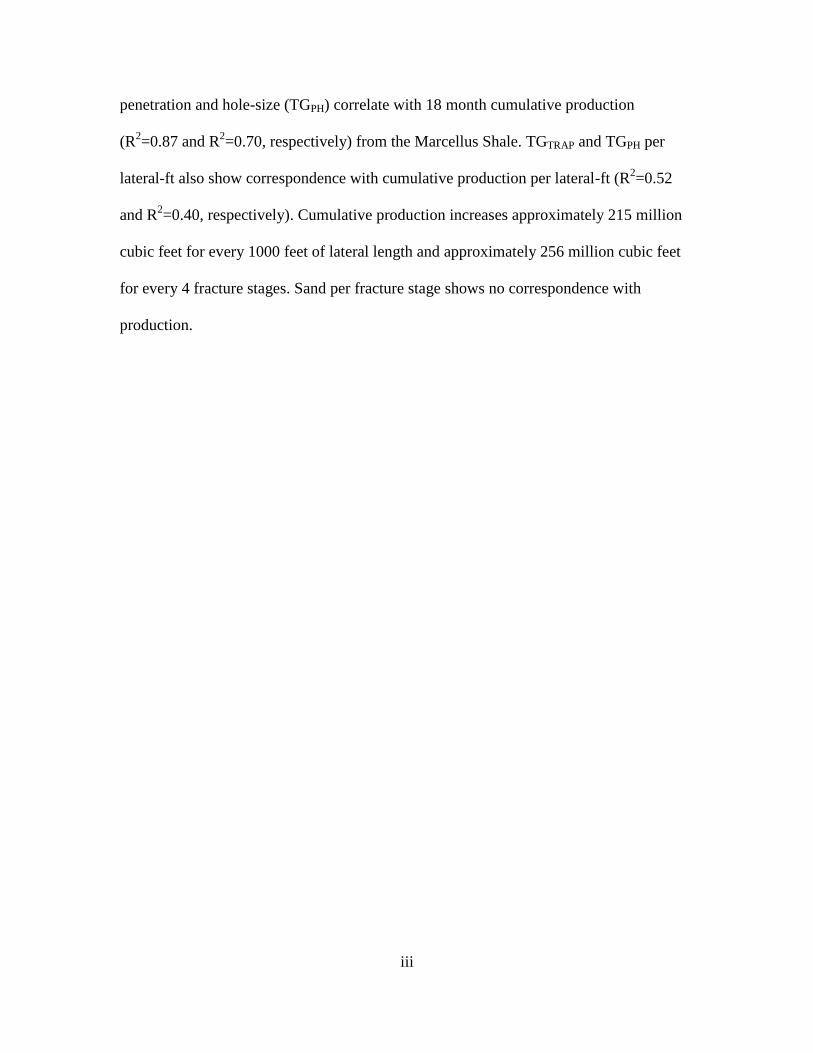
penetration and hole-size (TGPH) correlate with 18 month cumulative production

(R2=0.87 and R

2=0.70, respectively) from the Marcellus Shale. TGTRAP and TGPH per

lateral-ft also show correspondence with cumulative production per lateral-ft (R2=0.52

and R2=0.40, respectively). Cumulative production increases approximately 215 million

cubic feet for every 1000 feet of lateral length and approximately 256 million cubic feet

for every 4 fracture stages. Sand per fracture stage shows no correspondence with

production.

iv

ACKNOWLEDGEMENTS

Foremost, I would like to express my sincere gratitude to my advisor Dr. Castle

for his continuous support, guidance, motivation, and enthusiasm during this research. I

would also like to thank my committee members, Dr. Huddleston and Dr. Falta for their

insightful suggestions and willingness to help. My sincere thanks also go to Dr. Bridges

and Bill Donovan for their expertise and availability during this study.

I would also like to thank CONSOL Energy for kindly providing data and other

useful information needed to complete this study. Furthermore, I would like to thank the

Geology Team in Indiana, Pennsylvania for their encouragement, hard questions, and

graciousness in providing help.

Lastly and most importantly I would like to thank my parents and family for their

continuous, un-wavering support and love during my education. And to my wife, who

was patient, loving, encouraging, and vastly supportive.

v

TABLE OF CONTENTS

Page

ABSTRACT ........................................................................................................................ ii

ACKNOWLEDGEMENTS ............................................................................................... iv

LIST OF TABLES ............................................................................................................ vii

LIST OF FIGURES ......................................................................................................... viii

GLOSSARY ..................................................................................................................... xii

CHAPTER ONE: INTRODUCTION ................................................................................. 1

1.1 Background ............................................................................................................... 1

1.2 Research Significance and Objectives ...................................................................... 2

1.3 Organization of Thesis .............................................................................................. 3

1.4 References ................................................................................................................. 3

CHAPTER TWO: VERTICAL WELL INVESTIGATION: ASSESSING THE

MARCELLUS SHALE AT THE MAMONT PROSPECT USING CORE LAB

EQUATIONS AND THE SPECTRAL GAMMA-RAY LOG .......................................... 5

2.1 Abstract ..................................................................................................................... 5

2.2 Introduction ............................................................................................................... 5

2.3 Geologic Setting ........................................................................................................ 9

2.4 Methods ................................................................................................................... 11

2.5 Results ..................................................................................................................... 17

2.6 Discussion ............................................................................................................... 21

2.7 Conclusions ............................................................................................................. 24

2. 8 References .............................................................................................................. 25

CHAPTER THREE: CHAPTER THREE: HORIZONTAL WELL INVESTIGATION:

ASSESSMENT OF THE RELATIONSHIPS AMONG MUD-LOGGING GAS, WELL

DESIGN, AND PRODUCTION IN THE MARCELLUS SHALE ................................. 48

3.1 Abstract ................................................................................................................... 48

3.2 Introduction ............................................................................................................. 49

3.3 Geologic Setting ...................................................................................................... 53

3.4 Methods ................................................................................................................... 54

3.5 Results ..................................................................................................................... 61

vi

3.6 Discussion ............................................................................................................... 64

3.7 Conclusion ............................................................................................................... 67

3.8 References ............................................................................................................... 68

CHAPTER FOUR: CONCLUSIONS............................................................................... 86

APPENDICES .................................................................................................................. 89

vii

LIST OF TABLES

Page

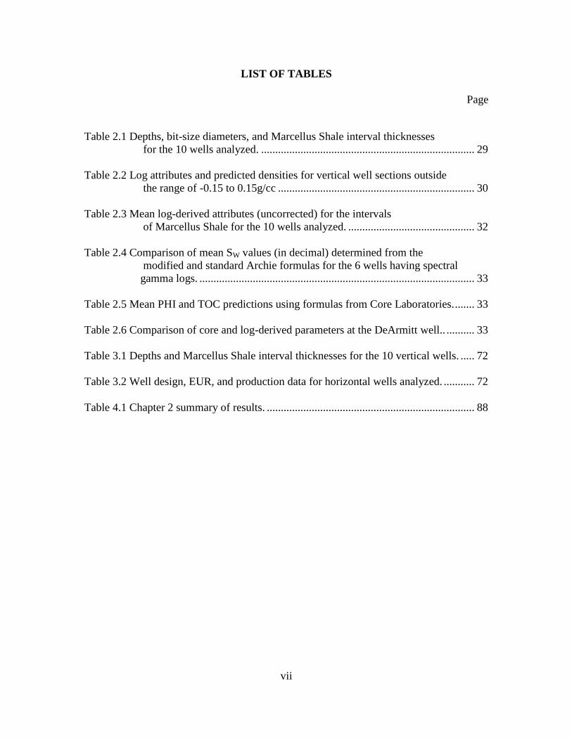
Table 2.1 Depths, bit-size diameters, and Marcellus Shale interval thicknesses

__________ for the 10 wells analyzed. ............................................................................ 29

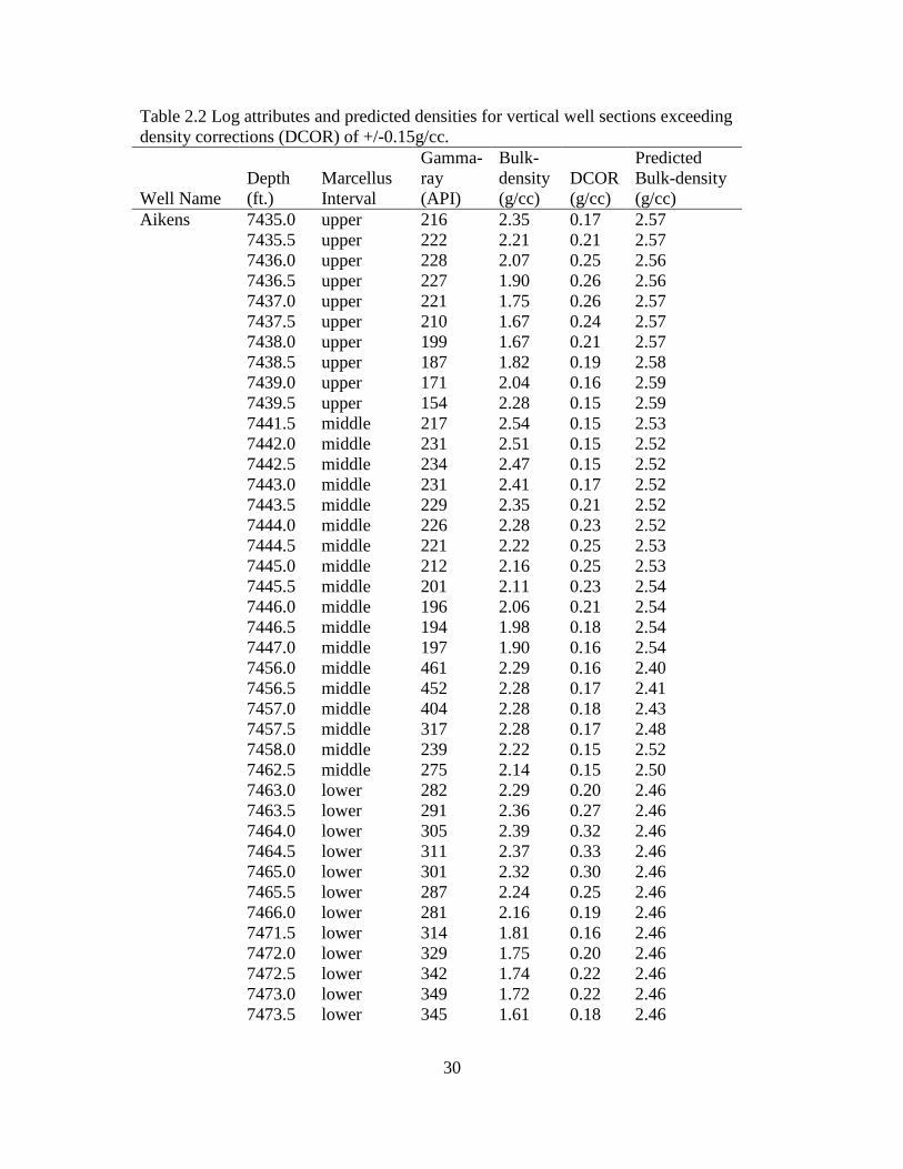
Table 2.2 Log attributes and predicted densities for vertical well sections outside

__________ the range of -0.15 to 0.15g/cc ...................................................................... 30

Table 2.3 Mean log-derived attributes (uncorrected) for the intervals

__________ of Marcellus Shale for the 10 wells analyzed. ............................................. 32

Table 2.4 Comparison of mean SW values (in decimal) determined from the

_ modified and standard Archie formulas for the 6 wells having spectral _

_ gamma logs. .................................................................................................. 33

Table 2.5 Mean PHI and TOC predictions using formulas from Core Laboratories. ....... 33

Table 2.6 Comparison of core and log-derived parameters at the DeArmitt well.. .......... 33

Table 3.1 Depths and Marcellus Shale interval thicknesses for the 10 vertical wells. ..... 72

Table 3.2 Well design, EUR, and production data for horizontal wells analyzed. ........... 72

Table 4.1 Chapter 2 summary of results. .......................................................................... 88

viii

LIST OF FIGURES

Page

Figure 2.1 Middle Devonian stratigraphy of southwestern Pennsylvania

_ (modified from Boyce, 2010). Upper, middle, and lower _ _ _

_ intervals of the Marcellus Shale are informal stratigraphic

_ units for the purpose of this study. .............................................................. 34

Figure 2.2 Vertical well type log of the Marcellus Shale at the Mamont

_ Prospect. Boundaries for the Marcellus Shale intervals were

_ picked using the gamma-ray log. The gamma-ray log is more

_ darkly shaded when 200 API is exceeded. The left side of the

_ log and the bold lines indicate the boundaries identified for

_ this study. The right side of the log and the dashed lines indicate

_ boundaries for the stratigraphic nomenclature of the type area for

_ the Marcellus Shale in New York. (Type log provided by

_ Energy) ........................................................................................................ 35

Figure 2.3 A= Regional map of study area location within Westmoreland

_ County, Pennsylvania. B= Local map of the Mamont Prospect

_ showing vertical well locations. .................................................................. 36

Figure 2.4 A= Linear regression model of bulk-density vs. gamma-ray. B= _

_ Logarithmic regression model of bulk-density vs. gamma-ray. ................. 37

Figure 2.5 Cross-section of the Bowman, Speer, and Hutchinson wells at the

_ Mamont Prospect. Stratigraphic boundaries of the Marcellus Shale _ _ _

_ intervals were picked using the gamma-ray log. MA= Mahantango

_ Shale UM= upper Marcellus; MM= middle Marcellus; LM= lower _

_ Marcellus; OL= Onondaga Limestone. Datum = Top Onondaga….……38

Figure 2.6 Marcellus Shale thickness map. An increase in thickness is observed

_ from the Germroth well in the west towards the Polahar and Kuhns

_ wells in the east-northeast. .......................................................................... 39

Figure 2.7 Top Marcellus Shale structure map. ................................................................ 39

Figure 2.8 Top Onondaga structure map. ......................................................................... 40

Figure 2.9 MLR model of bulk-density and gamma-ray. Data values were

_ obtained from non-rugose wells. Upper, middle, and lower are

_ references to the Marcellus intervals. ......................................................... 41

ix

Figure 2.10 Bulk-density vs. gamma-ray clusters separated into Marcellus

_ intervals. A= upper Marcellus interval; B= middle Marcellus

_ interval; C= lower Marcellus interval. Data values were obtained

_ from non-rugose wells. ............................................................................... 42

Figure 2.11 Isopach map of Marcellus Shale with gamma-ray > 230 API, which

_ has been recognized (Schmoker 1980) as the threshold between

_ organic-rich and organic-poor shale. .......................................................... 43

Figure 2.12 Isopach map of net productive Marcellus Shale, defined by gamma-

_ ray values >230 API and bulk-densities < 2.55 g/cc. ................................. 43

Figure 2.13 Iso SW (mod) map of net productive Marcellus Shale. Data points _

_ represent mean SW(mod) calculated for net productive Marcellus

_ Shale. ........................................................................................................... 44

Figure 2.14 Iso SW (std) map of net productive Marcellus Shale. Data points

_ represent mean SW(std) calculated for net productive Marcellus

_ Shale. ........................................................................................................... 44

Figure 2.15 Iso-porosity map of net productive Marcellus Shale. Data points

_ represent mean PHI calculated for net productive Marcellus

_ Shale. ........................................................................................................... 45

Figure 2.16 Isopach map of net productive Marcellus Shale with TOC greater

_ than 7%. ...................................................................................................... 45

Figure 2.17 Porosity-feet map of net productive Marcellus Shale, defined by

_ mean PHI of net productive Marcellus Shale * thickness of net

_ productive Marcellus Shale......................................................................... 46

Figure 2.18 Isopach map of Marcellus Shale with uranium content > 30 ppm. ............... 46

Figure 2.19 Uranium concentrations vs. gamma-ray (spectral) of the Marcellus

_ Shale at the Mamont Prospect for the 6 wells having spectral

_ gamma-ray logs. Uranium adsorbed by organic matter strongly _

_ influences shale radioactivity. ..................................................................... 47

Figure 3.1 Middle Devonian stratigraphy of southwestern Pennsylvania (modified

_ from Boyce, 2010). Uppe r, middle, and lower intervals of the

_ Marcellus Shale are informal stratigraphic units for the purpose

_ of this study……......................…………………………………………..73

x

Figure 3.2 A=Regional map showing study area location within _

_ Westmoreland County, Pennsylvania. B=Local map of the _

_ Mamont Prospect showing vertical and horizontal well locations. ........... 74

Figure 3.3 Vertical well type log of the Marcellus Shale at the Mamont _

_ Prospect (Hutchinson well, Figure 3.2 B). Boundaries for the _

_ Marcellus Shale intervals were picked using the gamma-ray log.

_ The gamma-ray log is more darkly shaded where 200 API is _

_ exceeded. The left side of the log and the bold lines indicate the _

_ boundaries identified for this study. The right side of the log and the

_ dashed lines indicate boundaries for the stratigraphic nomenclature

_ of the type area for the Marcellus Shale in New York. The basal

_ part of the Mahantango Shale is identified as the pronounced shelf

_ of gamma-radiation below 160 API overlying the upper Marcellus.

_ (Type log provided by CONSOL Energy) ................................................. 75

Figure 3.4 Complex depth shift performed on the Mountain vertical well and _

_ Hutchinson 4G horizontal well. LWD and wire-line gamma-ray

_ logs were stratigraphically aligned by adding tie lines to correlative

_ points from each log................................................................................... 76

Figure 3.5 TG calibrated on the basal part of the Mahantango Shale to 350 gas

_ units. Calibration was used to help disclaim inaccurate gas

_ response from mud-logging instrumentation (i.e., gas traps). TG

_ mean represents a mean TG value determined for each well’s LL.

_ TGTRAP mean represents a mean TG value after a zero adjustment

_ was performed. See Table 3.2 for well names and corresponding

_ well numbers. ............................................................................................. 77

Figure 3.6 A= Mean gamma-ray for Marcellus intervals. B= Mean penetration

_ for Marcellus intervals. .............................................................................. 78

Figure 3.7 Wire-line gamma-ray vs. LWD gamma-ray. A best-fit line yields

_ an R2

of 0.83. The resulting equation was used to determine

_ the threshold for shale of high gas content for LWD gamma-ray, a

_ boundary defined by Schmoker (1980) to be at 230 API (wireline).......... 79

Figure 3.8 A= Cumulative production vs. TG(TRAP) sum. B= Cumulative _

_ production per lateral-ft vs. TG(TRAP) per lateral-ft. ................................... 80

xi

Figure 3.9 A= Cumulative production vs. TG(PH) sum. B= Cumulative _

_ production per lateral-ft vs. TG(PH) per lateral-ft. ...................................... 81

Figure 3.10 A= Cumulative production vs. LL. B= Cumulative production vs.

_ number of fracture stages. .......................................................................... 82

Figure 3.11 Cumulative production per fracture stage vs. sand per fracture

_ stage. A weak correlation exists, thus no R2 was displayed. ..................... 83

Figure 3.12 A= Cumulative production vs. gamma-ray sum. B= Cumulative _

_ production per lateral-ft vs. gamma-ray per lateral-ft. ............................... 84

Figure 3.13 A= Cumulative production per lateral-ft vs. total feet (along LL) _

_ in middle interval divided by LL. B= Cumulative production

_ per lateral-ft vs. total feet in lower interval divided by LL. 9

_ of the 12 wells studied penetrated the lower interval. ............................... 85

xii

GLOSSARY

Bottom Lip – A feature of gas trap design that prevents drilling fluid from exiting the

trap bottom (Williams and Ewing, 1989).

Chromatography – Analytical process that entails the physical separation of gas

compounds from a gas mixture (e.g., drilling fluid) for identification and interpretation

(Whittaker, 2010). Before chromatographic analysis, the gas trap separates the gas

sample from the gas entrained in the drilling fluid.

Contamination Gas – Gas that has been artificially introduced into the drilling fluid, not

of formation rock origin (Mercer, 1974).

Estimated Ultimate Recovery (EUR) – Sum of all oil or gas that is forecast to have the

potential to be produced over the life of a well (Cook, 2003).

Fracture Stages – Sections of wellbore designated for hydraulic fracture treatment. Each

stage consists of multiple perforations that are treated at the same time. After treatment,

fracture connectivity is expected between stages.

Gas trap – Device used for the continual extraction of gases from the drilling fluid

(Whittaker, 2010). During sampling, gas traps do not capture all of the gas in the drilling

fluid and may capture certain gases at higher concentrations.

Lateral Length (LL) – Section of wellbore designated for hydraulic fracture treatment.

Includes all fracture stages and spaces between.

Liberated Gas – Mechanically liberated gas that enters the drilling fluid as the drill bit

penetrates and disaggregates the rock formation (Mercer, 1974). The gas in the drilled

volume consists of liberated gas and gas flushed ahead into the walls of the formation.

xiii

Measured Depth (MD) – Depth measured from the reference datum, typically the drill-

floor, along length of wellbore.

Mud-Logging – Standard practice for the evaluation of hydrocarbons returned to the

surface, entrained in the drilling fluid (Whittaker, 2010). Consisting of total gas,

chromatographic gas analysis, penetration, gamma-ray, and cutting description for both

lithologic characteristics and oil bound to cuttings.

Penetration – Time per unit depth of drill bit. Units are often given as inverse velocity in

min/ft. Recognized as an important indicator of rock strength and can be related to both

mineralogy and porosity (Whittaker, 2010).

Produced Gas – Gas produced into the drilling fluid as a result of formation pressure

exceeding opposing effective hydrostatic pressure (Mercer, 1974).

Recycled gas – Gas pumped down-hole that is brought to the surface a second time

(Mercer, 1974).

Total Depth (TD) – Total depth measured from the reference datum, typically the drill-

floor, along length of wellbore.

Total Gas (TG) – Sum of combustible gases determined from a total gas detector.

Detected components are typically of the low molecular-weight alkanes: methane [C1],

ethane [C2], propane [C3], butane [C4], and pentane [C5] (Whittaker, 1987).

Trip Gas – Gas that enters the borehole or drilling fluid by the swabbing action of the

drill string. As pipe is removed from the hole, well pressure can fall below formation

pressure causing an influx of gases (Adamson, 1998).

1

CHAPTER ONE: INTRODUCTION

1.1 Background

Shale gas reservoir development is an expanding source of natural gas reserves in

the United States (Arthur et al., 2008). The Marcellus Shale of the Appalachian Basin is

one shale gas play that is currently in the early phases of development (Arthur et al.,

2008). This unit is a low-permeability, organic-rich sedimentary rock that contains in

excess of 50 trillion cubic feet of natural gas (Engelder and Lash, 2008). The key to

economic extraction of natural gas from the Marcellus Shale is identifying locations of

the most producible hydrocarbons. Effective approaches in shale-gas reservoirs have

been to obtain in situ measurements by geophysical well-logging and to acquire

subsurface rock samples to reconstruct a lithological sequence (Serra, 1984). Parameters

related to porosity, lithology, hydrocarbons, and other rock properties can then be

obtained (Serra, 1984).

Geophysical well-logging can be defined as a record of rock characteristics

traversed by a measuring tool in the wellbore (Ellis and Singer, 2007). Measurements

may be of spontaneous phenomena, such as radioactivity. Or they may be induced, in

which a tool emits energy into the formation and measures the time it takes to reach a

receiver at a fixed distance along the tool (Rider and Kennedy, 2011). Since well logs are

available during drilling, logs are also used for geo-steering, such as keeping the bit

inside a thin reservoir, and evaluating down-hole conditions during and after drilling

(Rider and Kennedy, 2011). With the accessibility of well logs and the development of

numerous log analysis methods, shale-gas units such as the Marcellus Shale are being

2

evaluated extensively to further understand and interpret their potential to produce

hydrocarbons.

1.2 Research Significance and Objectives

At the Mamont Prospect in southwestern Pennsylvania, CONSOL Energy has

obtained mud logs and geophysical well logs from 10 vertical and 13 horizontal gas-

producing wells to aid in the extraction of natural gas from the Marcellus Shale. Study of

the relationships among these data and to production is important to understanding the

economic potential of current and future natural gas prospects in the Marcellus Shale. In

recent years, the renaissance in shale-gas production has required refinement of existing

methods and development of new techniques to predict reservoir properties that allow for

the evaluation of shale-gas units like the Marcellus Shale (Boyce, 2010). Boyce (2010)

characterized organic-rich shales using common well logs and the spectral gamma-ray

log from vertical wells. The relationship between gamma-ray and density-porosity was

evaluated and expanded to identify not only gas-rich zones of the Marcellus Shale, but

zones that may contain large volumes of producible gas. Boyce (2010) also re-evaluated

and modified the standard Archie formula to more accurately predict water and gas

saturations in the Marcellus Shale. Sexton (2011) integrated core data, geochemical

properties, and geophysical logs to create a predictive reservoir assessment of areas with

limited data control within the Marcellus Shale. Using data from unconventional CBM

wells in the Powder River Basin, Donovan (2003) related mud-logging gas content to

“back calculated” gas content from 2.5 years cumulative production. His study suggested

that mud-logging gas can be used as an indicator of well performance. The objectives of

this research were to 1) use existing log analysis methods to interpret Marcellus Shale

3

reservoir potential from vertical geophysical well-log data; and 2) assess relationships

among mud-logging gas, well design, and cumulative production data from horizontal

wells.

1.3 Organization of Thesis

This thesis is organized into four chapters including the Introduction (Chapter 1)

and Conclusions (Chapter 4). The two body chapters of this thesis are written and

formatted as independent manuscripts intended for submission to scientific journals for

publication:

Chapter 2: Vertical Well Investigation: Assessment of the Marcellus Shale at the

Mamont Prospect Using Equations from Core Laboratories and the Spectral

Gamma-ray Log

Chapter 3: Horizontal Well Investigation: Assessment of the Relationships

Among Mud-logging Gas, Well Design, and Production in the Marcellus

Shale

Chapter 2 concentrates on the most readily available geophysical well logs and the use of

formulas from Core Laboratories and those of previous studies to identify gas-rich

intervals of the Marcellus Shale. Chapter 3 is an evaluation of mud-logging gas data from

horizontal Marcellus wells. Cross-sections of the horizontally drilled wells are included

in the appendix.

1.4 References

Arthur, J. D., Bohm, B. & Layne, M. (2008). Hydraulic fracturing considerations for

natural gas wells of the Marcellus Shale. Ground Water Protection Council

Annual Forum.

4

Boyce, M. L. (2010). Sub-surface Stratigraphy and Petrophysical Analysis of the Middle

Devonian Interval of the Central Appalachian Basin; West Virginia and

Southwest Pennsylvania, PhD Dissertation, West Virginia University.

Donovan, W. (2007). Mudlogging Unconventional Gas Reservoirs. PowerPoint presented

at Unconventional Gas Technical Forum, Victoria, British Columbia, Canada,

Ministry of Energy, Mines and Petroleum Resources, 16 April.

Ellis, D.V. & Singer, J.M. (2007). Well logging for earth scientists. Netherlands:

Springer: Dordrecht, Netherlands.

Engelder, T. & Lash, G.G. (2008). Marcellus Shale play’s vast resource potential

creating stir in Appalachia. The American Oil and Gas Reporter, 7 pp., May.

Lee, D.S, Herman, J.D. & Elsworth, D.S. (2011). A Critical Evaluation of

Unconventional Gas Recovery From the Marcellus Shale, Northeastern United

States. Korean Society of Civil Engineers (KSCE) Journal of Civil Engineering

15(4): 679-687.

Rider, M. & Kennedy, M. (2011). The Geological Interpretation of Well Logs (3rd

ed.).

Scotland: Rider-French Consulting Ltd.

Serra, O. (1984). Fundamentals of Well-Log Interpretation: The Acquisition of Logging

Data, Amsterdam, Elsevier, Developments in Petroleum Science, vol. 1, 15 p.

Sexton, R. (2011). Sequence Stratigraphy, Distribution and Preservation of Organic

Carbon, and Reservoir Properties of the Middle Devonian Marcellus Shale of the

Central Appalachian Basin; Northern West Virginia and Southwestern

Pennsylvania, PhD Dissertation, West Virginia University.

5

CHAPTER TWO: VERTICAL WELL INVESTIGATION: ASSESSING THE

MARCELLUS SHALE AT THE MAMONT PROSPECT USING CORE LAB

EQUATIONS AND THE SPECTRAL GAMMA-RAY LOG

2.1 Abstract

The organic-rich interval of the Middle Devonian Marcellus Shale of the

Appalachian basin is a rapidly developing natural gas play. Using geophysical logs from

10 vertical gas-producing wells in Westmoreland County, Pennsylvania, stratigraphic

boundaries of the Marcellus Shale were identified. Gamma-ray, bulk density, and

resistivity well logs were examined to assess hydrocarbon potential at the Mamont

Prospect. Values of porosity, total organic carbon (TOC), and water saturation (SW) were

derived and mapped by incorporating well-log data into Marcellus-specific formulas.

The geophysical log data suggest increasing organic richness in 3 stratigraphically

descending Marcellus Shale intervals. Mean SW calculated from a modified Archie

formula range from 0.016 in the lower part of the Marcellus to 0.166 in the upper part,

compared to 0.121 and 0.314, respectively, calculated from the standard Archie formula.

Calculations from the bulk-density log yield 0.114 mean porosity and 6.9% mean TOC in

the lower part of the Marcellus. Coupling high gamma-ray values (>230 API) with low

bulk densities (< 2.55 g/cc) reveals a trend of increasing natural gas potential

southwestward within the Mamont Prospect.

2.2 Introduction

Unconventional resources comprise gas from tight sand, coal-bed methane, and

shale-gas (Bruner and Smosna, 2011) and oil from oil sands, heavy oil, and shale-oil

(Greene et al., 2004). In recent years, the resurgence in shale-gas production has required

fine-tuning of existing methodologies and development of new techniques to predict

6

reservoir attributes that allow for the evaluation of shale-gas reservoirs, such as the

Marcellus Shale of the Appalachian Basin (Boyce, 2010). While gas exploration and

production in the Marcellus Shale is fairly new, spanning just over 7 years (Bruner and

Smosna, 2011), relationships between well-log measurements and rock properties have

been identified. Where laboratory data are limited, log analyses for the evaluation of

organic-rich shales provide a practical interpretation of both location and quantity of

hydrocarbons present in shale-gas reservoirs. This study, an assessment of the Mamont

Prospect in Westmoreland County, Pennsylvania, focuses on interpreting the lateral

variability of log-derived parameters of the Marcellus Shale. The ultimate yield of natural

gas from the Marcellus Shale is estimated to be 489 trillion cubic feet (Engelder, 2009;

Pifer, 2010).

In Devonian shales, organic matter is the source of natural gas, and consequently

a measure of total gas generated (Schmoker, 1980). The quantity of organic matter is

usually expressed as total organic carbon (TOC) and can be measured directly via

laboratory analyses. TOC content of the Marcellus Shale in New York increases

westward from central to western New York where maximum values approach 6% (Hill

et al., 2004). A general decrease in TOC is observed from New York southward to West

Virginia (Milici and Swezey, 2006). A study by Repetski et al. (2002) determined TOC

content to be 3 to 6% in east-central Pennsylvania. In West Virginia the basal section of

the Marcellus Shale yields 8.8% maximum TOC and 5.2% mean TOC (Zielinski and

Nance, 1979). Regional variations in organic richness may reflect paleogeography of the

Acadian Delta where proximal parts (New York) show higher TOC content than distal

parts (West Virginia) (Milici and Swezey, 2006).

7

Although direct methods for determining source rock potential are more accurate

and preferred to indirect methods, well-logs offer continuous sampling of shale units

(Schmoker, 1980). The induction tool senses electrical conductivity to help differentiate

between conductive fluids (water or mud filtrate) and non-conductive fluids (oil or gas)

in a formation (Dewan, 1983). The density tool senses formation density by measuring

the attenuation of gamma-rays between a source and a detector (Dewan, 1983) and can be

useful for determining porosity. The gamma-ray tool measures natural radiation from

uranium, potassium, and thorium, which occur more abundantly in organic-rich shales,

such as the Marcellus Shale, than in higher permeability formations such as sandstones

and limestones (Dewan, 1983). Numerous studies have attempted to document the use of

well logs for recognizing and quantifying source rocks (Passey et al., 1990). A direct

relationship between gamma-ray intensity and organic matter content has been observed

in previous studies (Schmoker, 1980, 1981; Sondergeld et al., 2010). This relationship

provides a simple approach (i.e., by means of the gamma-ray log) for TOC

approximation. A better indicator of TOC, however, is bulk density because of the low

specific gravity of organic matter (Schmoker, 1979; Passey et al., 1990). It is from this

relationship that the bulk-density log is highly valued and commonly used for predicting

key reservoir parameters (i.e., porosity (PHI) and TOC) in organic-rich source rocks.

Core Laboratories Inc., a reservoir optimization company that provides patented

reservoir descriptions, among other services, has developed proprietary Marcellus-

specific formulas to predict PHI and TOC from the density log. These formulas were

derived by integrating sidewall-core and drill-cutting data with well-log data from

numerous Marcellus wells in three regions of the Appalachian Basin (i.e., northern,

8

central, and southern). They have been used and extended outside the cored interval

(within reason), and exported to other wells (Craig Hall, personal communication).

Conditions of the borehole environment (e.g., washout, rugosity, enlarged borehole),

however, can decrease accuracy of measurements made by the density tool. In rugose

boreholes, void space of collapsed formation material may influence bulk-density

measurement. To account for rugosity, the bulk-density log is usually accompanied by

the density-correction (DCOR) log, a recording of the absolute deviation of the log signal

(Benedictus, 2007). If this correction falls out-side of the range of -0.15 to 0.15 g/cc, the

bulk-density log is no longer trusted and measurements on these sections are ignored

(Dewan, 1983; Benedictus, 2007). Where density measurements are suspect, from

missing logs or borehole rugosity, the gamma-ray log can be converted to a pseudo-

density log, which can be used to calculate PHI and TOC (Schmoker, 1979, 1980, 1981;

Fertl and Chilingar, 1988). Soeder (1988) determined mean PHI values within the

Marcellus Shale to be near 10%.

Gamma-ray intensity has been attributed to uranium concentration associated with

organic matter (Russell, 1945; Swanson, 1960; Zelt, 1985; Passey et al., 1990; Lüning

and Kolonic, 2003; Boyce, 2010). This empirical observation has increased the viability

and use of the spectral gamma-ray tool, an instrument that determines the concentrations

of components (i.e., uranium, thorium, and potassium) contributing to gamma radiation.

In a previous study of Devonian shales, Boyce and Carr (2009) recognized a relationship

between increased uranium concentrations from spectral gamma-ray logs and increased

TOC, and related increased gas content to increased TOC, consequently providing a

relationship between uranium concentration and gas production potential. Boyce (2010)

9

and Yanni (2010) used these relationships to identify high gas potential zones of the

Middle Devonian interval, including the Marcellus Shale, at basin-wide scales. Boyce

(2010) also estimated regional water saturations (SW) by re-evaluating and modifying the

standard Archie formula to include concentrations of thorium and uranium. Without

thorium and uranium, the standard Archie formula, originally developed in a shale-free

lithology, yields an over-estimation of SW in the Marcellus Shale (Boyce, 2010). Clay-

bound water is suggested by Boyce (2010) as the chief contributor to this over-

estimation. Although SW is not of primary interest in the Marcellus Shale, it can be useful

in determining zones of increased hydrocarbon saturation (i.e., low SW) (Coughlin, 2009).

The approach of this study is to assess the lateral variability of key reservoir

parameters of the Marcellus Shale at the Mamont Prospect using data from geophysical

logs of vertical wells and formulas derived by Boyce (2010) and Core Laboratories. The

approach includes assessing applicability of basin-wide studies by Boyce (2010) and

Yanni (2010) to the Mamont Prospect. The objectives of this study were to 1) assess the

Marcellus Shale in the Mamont Prospect using gamma-ray, bulk density, and resistivity

well-log data; 2) calculate and map PHI, TOC, and SW by integrating log data with

recently developed Marcellus-specific formulas; 3) compare formula-derived PHI, TOC,

and SW to measured core data; and 4) assess applicability of the techniques described by

Boyce (2010) and Yanni (2010) to the Mamont Prospect.

2.3 Geologic Setting

The Appalachian Basin is a northeast-southwest trending foreland basin that was

formed during the Middle to Late Ordovician Taconic orogeny (Faill, 1997). During the

Acadian Orogeny (Middle Devonian), basin filling was dominated initially by organic-

10

rich black shale, a consequence of paleoclimatic and paleogeographic constraints

(Ettensohn, 1987). The author proposed that deposition of black shale occurred when

basins were deepest, most restricted, and received least sediment. Deep, anoxic

conditions represented by the shale and the sharp contact between basal units suggest the

basins were formed during periods of abrupt subsidence (Ettensohn, 1987). It has also

been proposed that black shale was deposited in an epeiric sea of a shallow basin,

allowing for the preservation of organic material through anaerobic conditions

(Schwietering, 1981).

Comprised of two black shale units separated by limestone, shale, and sandstone,

the Middle Devonian Marcellus Shale Formation occurs in the basal Hamilton Group, an

east to southeastward thickening succession of marine and non-marine shale, siltstone,

and sandstone (Lash and Engelder, 2011). The Marcellus Shale in New York (i.e., the

type area for the Marcellus Shale) comprises, in stratigraphically ascending order, the

Union Springs, Cherry Valley, and Oatka Creek members. The Union Springs Member is

a radioactive, low-density shale directly above the Onondaga Formation (Lash and

Engelder, 2011). The Cherry Valley Member consists of nodular limestone, shale, and

siltstone, and is recognized by low radioactivity (Lash and Engelder, 2011). The Oatka

Creek Member is recognized by a radioactive basal section and a less radioactive, higher

density upper section (Lash and Engelder, 2011). In southwestern Pennsylvania, the

Oatka Creek and Union Springs members are typically referred to as the Upper and

Lower Marcellus Shale members and are separated by the Purcell Limestone, a

correlative of the Cherry Valley Member (Lash and Engelder, 2011). For this

11

investigation, three informal stratigraphic intervals (i.e., upper, middle, and lower) of the

Marcellus Shale were defined (Figures 2.1 and 2.2).

Extending from Ohio to Pennsylvania, the Marcellus Shale varies from 50 to 200

feet in thickness and occurs 1,000 to 7,000 feet below the top of Devonian strata (Soeder,

2010). The Marcellus Shale is predominantly gray-black to black, thinly laminated, non-

calcareous, and fissile (Boyce, 2010). Analyses of core samples via x-ray diffraction

reveal high quartz content (60%), low clay content (30%), and pyrite (10%) (Boyce,

2010). Within the Mamont Prospect the Marcellus Shale underlies the Middle Devonian

Mahantango Shale, a variable mix of mudstone, sandstone, limestone, and conglomerate

(Bruner and Smosna, 2011), and occurs atop limestone of the Middle Devonian

Onondaga Formation. The Mamont Prospect contains 10 vertical gas-producing wells

within an area of 9 square miles (Figure 2.3; Table 2.1).

2.4 Methods

2.4.1 Assessing the Marcellus Shale Using Well Logs

The Marcellus Shale was assessed by 1) importing well-log LAS files into

GeoGraphix®; 2) identifying Marcellus Shale stratigraphic boundaries using the gamma-

ray log; 3) correcting bulk-density measurements in rugose boreholes using a relationship

between gamma-ray and bulk density; and 4) using gamma-ray, bulk-density, and

resistivity logs to identify high gas-potential zones.

2.4.1.1 Data Collection and Preparation

Drilling start dates for the 10 wells studied at the Mamont Prospect occurred

between May 2008 and November 2009. All wells were drilled on air. Digital and LAS

(Log ASCII Standard) files containing depths, geophysical logs, and other well

12

parameters were produced and updated during the drilling process by CONSOL Energy.

Schlumberger Inc. assisted CONSOL Energy in drilling and operations of the DeArmitt

well, and Weatherford Inc. assisted with the other wells. After drilling, CONSOL Energy

imported LAS files into GeoGraphix® software.

2.4.1.2 Identifying Stratigraphic Boundaries of the Marcellus Shale

In XSection, a GeoGraphix®

module, stratigraphic tops were ‘picked’ at gamma-

ray inflection points for the Onondaga Limestone and the 3 intervals (upper, middle, and

lower) of Marcellus Shale (Figure 2.2). A cross-section of the 10 wells studied was

created and used as reference to maintain consistency in picks from well-to-well. Each

Marcellus Shale interval is separated by a zone of low gamma radiation. The top of the

upper Marcellus interval was picked at the base of the Mahantango Shale beneath a

pronounced shelf of gamma radiation below 160 API. Similarly, the Onondaga

Limestone was picked at the top of a pronounced shelf of gamma radiation below 160

API. The middle and lower Marcellus intervals were each picked at the base of a

decreased API response directly below an API kick. Gamma-ray values peak at 320 to

360 API for the upper Marcellus, 440 to 480 API for the middle Marcellus, and 700 to

760 API for the lower Marcellus. Well positions were imported into Surfer® from

GeoGraphix® to generate a location map for the 10 wells studied. Structure contour maps

for the top Onondaga Limestone and top Marcellus Shale were contoured by hand using

ground elevations and formation thicknesses.

2.4.1.3 Bulk-density Corrections in Rugose Sections of Borehole

The caliper and bulk-density logs for the 10 wells studied were visually

examined. At equivalent depths, changes in borehole size were linked to deviations along

13

the bulk-density log. From this observation, the caliper log was used as the primary tool

for rugose borehole identification. Sections of borehole where the diameter from the

caliper log exceeded 10% of the bit-size (an arbitrary value selected for this study) were

considered rugose. Since gamma-ray is not sensitive to borehole conditions (e.g.,

washout, rugosity, enlarged borehole), and to delineate an acceptable prediction model

that uses gamma-ray as a proxy for bulk-density, regression analyses were performed.

Wells with 10 or more feet of rugose borehole (DeArmitt, Aikens, and Kuhns) were not

used in order to prevent effects of unrepresentative data. From the complete data set, the

simple linear regression model (Figure 2.4 A) and the logarithmic regression model

(Figure 2.4 B) yield weak-to-moderate correlation coefficients (R2=0.31 and R

2=0.41,

respectively), and do not adequately fit data values across the models. As observed from

the type log (Figure 2.2), the gamma-ray response peaks at higher API values in

stratigraphically descending Marcellus intervals. Therefore, under the assumption that

bulk-density decreases with increasing gamma-ray, JMP (statistical analysis software

developed by SAS) was used to create a multiple linear regression (MLR) model,

governed by the expression in Equation 1.

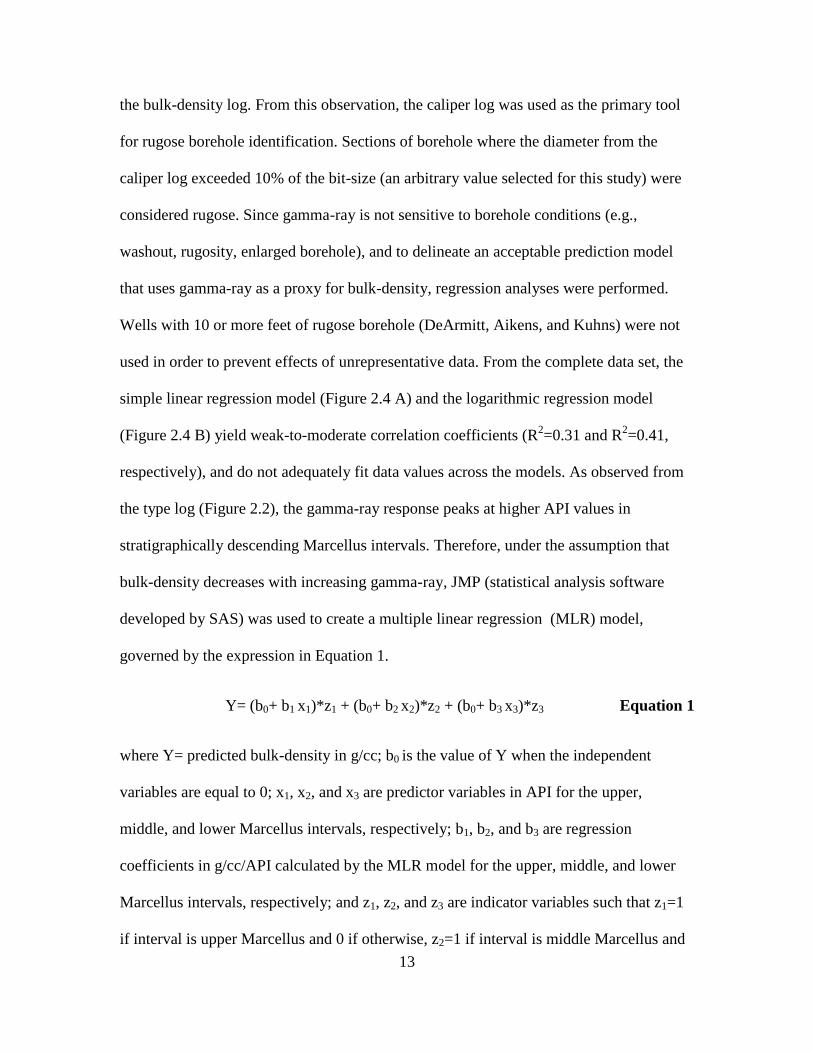
Y= (b0+ b1 x1)*z1 + (b0+ b2 x2)*z2 + (b0+ b3 x3)*z3 Equation 1

where Y= predicted bulk-density in g/cc; b0 is the value of Y when the independent

variables are equal to 0; x1, x2, and x3 are predictor variables in API for the upper,

middle, and lower Marcellus intervals, respectively; b1, b2, and b3 are regression

coefficients in g/cc/API calculated by the MLR model for the upper, middle, and lower

Marcellus intervals, respectively; and z1, z2, and z3 are indicator variables such that z1=1

if interval is upper Marcellus and 0 if otherwise, z2=1 if interval is middle Marcellus and

14

0 if otherwise, z3=1 if interval is lower Marcellus and 0 if otherwise. Where DCOR

values along rugose boreholes exceeded 0.15 or -0.15g/cc, new bulk-density values were

estimated using the predictor equation (Equation 1).

2.4.1.4 Identifying High Gas-Potential Zones

To assess variability with depth, mean values of gamma-ray, bulk density and

resistivity for each well were calculated for the upper, middle, and lower Marcellus Shale

intervals. Schmoker (1980) suggested a gamma-ray value of 230 API as a boundary

between organic-rich and organic-poor shale and a threshold value for shale of high gas

content. Therefore, an isopach map of Marcellus Shale with gamma-ray greater than 230

API was created. Schmoker (1981) noted, however, that quantitative interpretation of

organic-matter content from the gamma-ray log requires a covariance between gamma-

ray and bulk-density (i.e., where gamma-ray increases with decreasing bulk density). For

this study, gamma-ray greater than 230 API and bulk density less than 2.55 g/cc were

considered threshold values of Marcellus Shale that contribute to production. Therefore,

net productive Marcellus Shale thickness was determined by applying cut-offs of gamma-

ray (> 230 API) and bulk density (< 2.55 g/cc). An isopach map of net productive

Marcellus Shale was created. Values for isopach maps were calculated to the nearest 0.5

ft.

2.4.2 Calculating and Mapping SW, PHI, and TOC

SW was calculated using a modified Archie formula and the standard Archie

formula. PHI and TOC were calculated using formulas from Core Laboratories.

15

2.4.2.1 SW Calculation

The standard Archie formula, developed to predict water and gas saturations using

data from petrophysical measurements, was originally derived in a shale-free lithology.

This equation relates resistivity of a rock to its porosity, water resistivity of its saturated

pores, and fractional SW of pore space (Archie, 1942; Dewan, 1983). The use of this

equation in shale-gas reservoirs, however, can produce inaccurate estimation of SW, and

overestimation has been attributed to suppressed resistivity from clay-bound water in

shales (Boyce, 2010). Developed by Boyce (2010), a modified Archie formula (Equation

2) incorporates components of the spectral gamma-ray log (i.e., thorium and uranium) to

account for clay-bound water. For each of the 6 wells (Weister, Bowman, Germroth,

Speer, Polahar, Mountain) having spectral gamma-ray logs, Equation 2 was used to

calculate SW on a foot-by-foot basis. For comparison, SW was also calculated on a foot-

by-foot basis using the standard Archie formula (Equation 3).

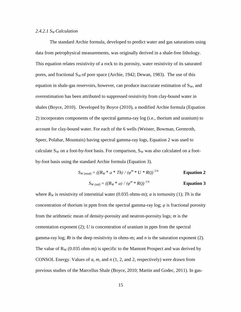
SW (mod) = ((RW * a * Th) / (φm

* U * Rt)) 1/n

Equation 2

SW (std) = ((RW * a) / (φm

* Rt)) 1/n

Equation 3

where RW is resistivity of interstitial water (0.035 ohms-m); a is tortuosity (1); Th is the

concentration of thorium in ppm from the spectral gamma-ray log; φ is fractional porosity

from the arithmetic mean of density-porosity and neutron-porosity logs; m is the

cementation exponent (2); U is concentration of uranium in ppm from the spectral

gamma-ray log; Rt is the deep resistivity in ohms-m; and n is the saturation exponent (2).

The value of RW (0.035 ohm-m) is specific to the Mamont Prospect and was derived by

CONSOL Energy. Values of a, m, and n (1, 2, and 2, respectively) were drawn from

previous studies of the Marcellus Shale (Boyce, 2010; Martin and Godec, 2011). In gas-

16

bearing formations, porosity measured from the bulk-density log is highly over-estimated

(i.e., high density-porosity) from gas present in pore space (Benedictus, 2007). In

contrast, neutron-porosity is highly under-estimated, as the hydrogen index of gas is

much lower than that of water (Rider, 1986; Benedictus, 2007). This anomaly has been

coined “the gas effect,” and can be corrected by averaging density-porosity and neutron-

porosity logs (Benedictus, 2007). For each of the 6 wells having spectral gamma-ray logs,

a mean SW (mod) and a mean SW (std) were calculated (expressed as a decimal) for the 3

intervals of Marcellus Shale and for net productive Marcellus Shale. Using these data, SW

(mod) and SW (std) iso-maps were created for net productive Marcellus Shale.

2.4.2.2 PHI and TOC Calculations

For three regions of the Appalachian Basin (i.e., northern, central, and southern),

X-ray diffraction (XRD), TOC, PHI, permeability, and SW data (i.e., from sidewall-core

and drill cuttings) were collected by Core Laboratories to compare with log response of

the Marcellus Shale. After applying a core-to-log depth-shift, Core Laboratories cross-

plotted the core data (i.e., data derived from sidewall-core and drill cuttings) with the log

data to generate proprietary algorithms to calculate PHI and TOC based on the best

correlation between any two parameters (Craig Hall, personal communication). Upon

approval by Core Laboratories, bulk-density log data from the 10 Mamont wells were

integrated into the central region formulas to calculate PHI and TOC on a foot-by-foot

basis. For each of the 10 wells, mean PHI (expressed as a decimal) and mean TOC

(expressed as a %) were calculated for the 3 Marcellus intervals. Mean PHI was

calculated for net productive Marcellus Shale to create an isoporosity map. An isopach

map of TOC greater than 7% was contoured for net productive Marcellus Shale. An

17

isovolume map of porosity-ft for net productive Marcellus Shale was created (i.e., net

productive Marcellus Shale thickness * mean PHI of net productive Marcellus Shale).

2.4.3 Comparing Core and Log-derived PHI, TOC and SW Data

PHI, TOC, and SW were measured in 3 plugs obtained from different depths in

conventional cores from the DeArmitt well by Terra Tek, a Schlumberger company. The

core measurements were compared to PHI, TOC, and SW values calculated using

formulas from Core Laboratories and Equation 3.

2.4.4 Assessing Applicability to the Mamont Prospect

To assess applicability of results to the Mamont Prospect, the isopach map of

Marcellus Shale with gamma-ray > 230 API and the isopach map of net productive

Marcellus Shale with TOC greater than 7% were compared to interpretations made by

Boyce (2010) and Yanni (2010). Boyce (2010) and Yanni (2010) identified gas-rich

intervals of the Marcellus Shale using relationships between gamma-ray intensity,

uranium concentrations, and TOC content. To aid in this comparison, an isopach map of

Marcellus Shale with uranium concentrations > 30 ppm was contoured from the 6 wells

having spectral gamma-ray logs.

2.5 Results

2.5.1 Hydrocarbon Potential of Marcellus Shale Using Common Well Logs

2.5.1.1 Data Collected

Total depths (TD), measurements in feet from ground level along length of

wellbores, ranged from 7,575 to 7,973 feet (Table 2.1). Measurements of gamma-ray,

bulk density, and resistivity were recorded at 0.5 foot increments.

18

2.5.1.2 Stratigraphic Boundaries of the Marcellus Shale

Stratigraphic boundaries, defined in cross-section using the gamma-ray log

(Figure 2.5), revealed that Marcellus Shale thickness ranges from 88.5 to 98 feet. The

Marcellus Shale thickens eastward from west Mamont (Figure 2.6). A structure map of

the Marcellus Shale reveals a northwest-southeast trend, with structurally deeper

Marcellus Shale in the southwest (Figure 2.7), coinciding with the structural trend of the

Onondaga Limestone (Figure 2.8).

2.5.1.3 Bulk-density Corrections in Rugose Sections of Borehole

For the 3 rugose wells (DeArmitt, Aikens, and Kuhns) DCOR measurements

applied to bulk-density logs indicated a total of 41 feet of borehole having suspect bulk-

density values (i.e., DCOR falling out of the range of -0.15 to 0.15g/cc). 20 feet of this

total were from sections located in the middle Marcellus interval of the Aikens well

(Table 2.2). The MLR model (Figure 2.9), governed by Equation 1, resulted in a

combined R2 that explains 67% (R

2=0.67) of the variability between bulk-density and

gamma-ray. The p-value (i.e., significance level) associated with this model is less than

0.0001. This indicates that the p-value is less than alpha (i.e., an arbitrary level of risk

assumed at 0.05), and consequently disproves the null hypothesis (i.e., a general position

that there is no relationship between two measured phenomena). Bulk-density values

predicted from the MLR model ranged from 2.40 to 2.59 g/cc (Table 2.2). Plots of bulk-

density vs. gamma-ray for each Marcellus interval are shown in Figure 2.10.

2.5.1.4 High Gas Potential Zones

Among the 10 wells studied, mean values for gamma-ray, bulk density, and

resistivity for the Marcellus Shale ranged from 284–325 API, 2.49–2.52 g/cc, and 72–127

19

ohms-m, respectively (Table 2.3). Among the 3 Marcellus Shale intervals, mean gamma-

ray and resistivity values were highest in the lower interval, ranging from 385–442 API

and 110–212 ohms-m, respectively. Values of mean bulk-density were lowest in the

lower interval and ranged from 2.42–2.48 g/cc. Marcellus Shale thickness with gamma-

ray > 230 API (Figure 2.11) is greatest in west-northwest Mamont in the vicinity of the

Mountain well (67 ft.). Thickness of net productive Marcellus Shale (Figure 2.12)

indicates a trend of increasing gas potential southwestward across the Mamont Prospect.

2.5.2 Mapping PHI, TOC, and SW

2.5.2.1 SW Calculation

Among the 6 wells having spectral gamma-ray logs, mean values of SW (mod) and

SW (std) for the Marcellus Shale ranged from 0.077–0.098 and 0.216–0.253, respectively

(Table 2.4). Among the 3 intervals of Marcellus Shale, mean values of SW (mod) and SW (std)

were lowest in the lower interval and ranged from 0.016–0.037 and 0.121–0.178,

respectively. Mean SW (mod) and SW (std) calculated for net productive Marcellus Shale, is

lowest (i.e., highest gas saturation) in south Mamont in the vicinity of the Bowman well

(0.036 and 0.136, respectively) and increases towards the Germroth well (0.055 and

0.179, respectively) in the west and the Polahar well (0.052 and 0.193, respectively) in

the east (Figures 2.13 and 2.14).

2.5.2.2 PHI and TOC Calculation

Among the 10 wells studied, mean values for PHI and TOC for the Marcellus

Shale ranged from 0.084-0.096 and 5.1-5.8% by weight, respectively (Table 2.5). Among

the 3 Marcellus Shale intervals, mean PHI and TOC values were highest in the lower

interval, ranging from 0.097-0.114 and 5.9-6.9% by weight, respectively. Mean PHI and

20

thickness with TOC greater than 7% for net productive Marcellus Shale (Figures 2.15 and

2.16) are greatest in north Mamont in the vicinity of the Aikens well (0.111 and 23.5 ft.,

respectively) and lowest in the vicinity of the Germroth well (0.097 and 4.5 ft.,

respectively) and Polahar well (0.097 and 4 ft., respectively). Figure 2.17 reveals a trend

of increasing porosity-ft for net productive Marcellus Shale from northeast Mamont

towards the southeast.

2.5.3 Comparison of Core and Log-derived PHI, TOC and SW Data

PHI and TOC values measured in cores from the DeArmitt well ranged from

0.056-0.073 and 5.2-8.0% by weight, respectively (Table 2.6). At the same depths as the

3 cores, PHI and TOC values calculated using proprietary formulas from Core

Laboratories ranged from 0.109-0.125 and 6.6-7.3% by weight, respectively. SW values

measured from core ranged from 0.230- 0.388, and SW values calculated from the

standard Archie formula (Equation 3) ranged from 0.090-0.154.

2.5.4 Applicability to the Mamont Prospect

Boyce (2010) and Yanni (2010) found that Marcellus Shale gross thickness does

not correlate strictly with Marcellus Shale thickness having high gamma radiation. At the

Mamont Prospect, Marcellus thickness with gamma radiation >230 API (Figure 2.11)

increases towards the west, opposite to the direction of increasing gross thickness (Figure

2.6). Boyce (2010) and Yanni (2010) also determined that net thickness of Marcellus

Shale having uranium concentrations >15 ppm correlates with net thickness of Marcellus

Shale having gamma-ray values >230 API. At the Mamont Prospect, from the 6 wells

having spectral gamma-ray logs, net Marcellus thickness with uranium concentrations >

30 ppm thickens from the Bowman well in the south (42.5 ft.) towards the Germroth well

21

in the west (55 ft.) (Figure 2.18), closely following the trend of thickening Marcellus

Shale with elevated gamma radiation (>230 API). A polynomial relationship between

TOC (core-measured) and uranium concentrations (spectral gamma-ray) were used by

Boyce (2010) and Yanni (2010) to identify TOC rich areas of the Appalachian basin.

2.6 Discussion

A well-established relationship between increased gamma-ray and increased TOC

has been defined in previous studies (Swanson, 1960; Schmoker, 1981; Fertl and

Chilingar, 1988). Correlation between organic matter content and gamma-ray within

Devonian shales reflects the association of uranium with organic matter (Schmoker,

1981), providing a link between uranium concentration and gamma ray. At the Mamont

Prospect, uranium adsorbed by organic matter strongly influences shale radioactivity

(Figure 2.19). This relationship likely exists because uranium is easily adsorbed by

carbonaceous material, predominantly in reducing environments where hexavalent

uranium (U+6

) reduces to U+4

(Fertl and Chilingar, 1988). Other factors include 1)

uranium concentration in seawater during deposition; 2) type of organic matter deposited;

3) water chemistry at the water-sediment boundary; and 4) sedimentation rate (Schmoker,

1981). For the 10 wells studied, mean gamma-ray values calculated for the Marcellus

Shale intervals increase in stratigraphically descending order (Table 2.3), indicating

increased uranium concentration and increased TOC with depth.

Due to its low specific gravity, organic matter content can have a profound

influence on bulk density calculated from well logs (Meyer and Nederlof, 1984). Boyce

(2010) identified an overall increase in well-log bulk-density with decreasing TOC

measured from core samples. The bulk-density log has been observed to have a well-

22

defined relationship with the gamma-ray log (Schmoker, 1979, 1980, 1981; Fertl and

Chilingar, 1988). In the western Appalachian Basin, Schmoker (1979) established a linear

relationship (R2=0.86) between gamma-ray and bulk-density values. Where bulk-density

logs were missing, Schmoker (1979) accurately estimated TOC measured from core

samples using pseudo-density values generated from the gamma-ray log. Similarly, at the

Mamont Prospect, the MLR model (Figure 2.9) produces a strong relationship (R2=0.67)

between bulk density and gamma-ray. The MLR model utilizes the relationships

observed in the models for the individual intervals (Figures 2.10 A, B, and C) to create a

model that is more accurate for calculating bulk-density from gamma-ray than the linear

and logarithmic regression models (Figures 2.4 A and B). Bulk-density values calculated

for the Marcellus Shale intervals decrease in stratigraphically descending order (Table

2.3), consistent with increased TOC with depth.

Organic carbon is electrically non-conductive, making the induction tool a viable

instrument in source rock evaluation. In any given formation where oil or gas (i.e., non-

conductive fluid) is present in sufficient quantities, water is displaced, resulting in higher

resistivity values (Passey et al., 2010). For the 10 wells studied, mean resistivity values

determined for each Marcellus Shale interval increase in stratigraphically descending

order (Table 2.3), indicating increased TOC with depth.

Boyce (2010) hypothesized that the modified Archie formula estimates a more

accurate SW than the standard Archie formula in formations where clay-bound water

causes underestimation of hydrocarbon saturation. To reduce this effect, Boyce (2010)

incorporated uranium and thorium into the standard Archie formula, supported by

relationships between uranium concentration and gas content, and thorium and resistivity.

23

SW calculated using the modified Archie formula (Equation 2) suggests that mean SW at

the Mamont Prospect for the Marcellus Shale intervals range from 0.016 in the lower

Marcellus to 0.166 in the upper Marcellus; compared to 0.121 and 0.314, respectively,

using the standard Archie formula (Equation 3).

Passey et al. (2010) explained that TOC content (%) by volume is nearly 2 times

TOC content (%) by weight in rocks. In some cases, 5% TOC by weight may correspond

to a volume % up to four times its weight % (Passey et al., 2010). At the Mamont

Prospect, +/-1.4% by weight (maximum deviation) is observed between core-measured (3

samples) and log-derived TOC (Table 2.6), which is consistent with a study by Passey et

al. (1990), in which a standard deviation of measured TOC and log-derived TOC was +/-

1.2% in gas-bearing formations.

Boyce (2010) and Yanni (2010) proposed that gas-rich intervals in the Marcellus

Shale are best identified by considering both thickness and gamma-ray (>230 API).

Structural highs and lows of the underlying Onondaga Limestone were hypothesized by

Boyce (2010) and Yanni (2010) to control regional distribution of TOC within the

Appalachian Basin. They observed that structural lows of the Onondaga Limestone

correspond to increased Marcellus Shale organic richness (TOC interpreted from

increased net uranium) and interpreted areas of highest TOC to be related to the

underlying structure during deposition. At the Mamont Prospect, Marcellus Shale with

gamma-ray >230 API (Figure 2.11) is thickest in west-northwest Mamont (67 ft.),

coinciding with Marcellus Shale thickness with uranium concentrations >30 ppm (Figure

2.18). Comparing gamma-ray >230 API and uranium concentration >30 ppm to the

Onondaga Limestone structure map (Figure 2.8), it appears that structural lows may

24

control distribution of Marcellus Shale organic richness in the Mamont Prospect. By

combining high gamma-ray values (> 230 API) and low bulk-densities (< 2.55 g/cc) (i.e.,

net productive Marcellus Shale), a trend of increased gas potential is observed from

northeast Mamont towards the southwest (Figure 2.12) and follows more closely

structural deepening of the Onondaga Limestone (Figure 2.8) than does stand-alone

gamma-ray (Figure 2.11).

Derived from the bulk-density log using formulas from Core Laboratories, mean

PHI and TOC iso-maps of net productive Marcellus Shale suggest that gas potential is

greater in the vicinity of the Aikens well than in other areas within the Mamont Prospect

(Figures 2.15 and 2.16). A porosity thickness map (i.e., mean phi of net productive

Marcellus Shale * thickness of net productive Marcellus Shale), however, reveals a trend

of increased gas potential from northeast to southwest Mamont (Figure 2.17); a trend that

follows dip-direction of the Marcellus Shale and Onondaga Limestone.

2.7 Conclusions

To improve accuracy in estimations of TOC within the Mamont Prospect, pseudo-

density values were estimated from gamma-ray logs to replace potentially inaccurate

bulk-density values in rugose sections of borehole. Calculated mean values of gamma-

ray, bulk density, and resistivity suggest increased organic richness in stratigraphically

descending Marcellus Shale intervals. This investigation is the first known study to

define 3 informal stratigraphic units of the Marcellus Shale (upper, middle, lower); a

methodology adopted from CONSOL Energy. The modified Archie formula from Boyce

(2010) yields a 0.016 mean SW in the lower Marcellus and 0.166 mean SW in the upper

Marcellus, compared to 0.121 and 0.314, respectively, calculated from the standard

25

Archie formula. Formulas from Core Laboratories yielded 0.114 mean PHI and 6.9%

mean TOC calculated from the bulk-density log in the lower Marcellus interval. A trend

of increased natural gas potential in the Mamont Prospect corresponds to structural

deepening of the underlying Onondaga Limestone. Within the Mamont Prospect,

increased natural gas potential does not correspond to gross Marcellus Shale thickness,

but to net productive Marcellus Shale thickness defined by gamma-ray >230 API and

bulk density < 2.55 g/cc. Mapping of porosity-ft was used in this study to evaluate the

areal distribution of gas reservoir. Porosity-ft of net productive Marcellus Shale is

greatest in the vicinity of the Weister and Speer wells and closely follows the

southwestward trend of structural deepening of the Onondaga Limestone.

2. 8 References

Archie, G. E. (1942). The electrical resistivity log as an aid in determining some reservoir

characteristics. Trans. AIMe, 146(1), 54-67.

Benedictus, T. (2007). Determination of petrophysical properties from well logs of the

offshore Terschelling Basin and southern Central North Sea Graben region (NCP-

2A) of the Netherlands. TNO Report 2007-U-R0169/A, TNO, 53 p.

Boyce, M. L. (2010). Sub-surface Stratigraphy and Petrophysical Analysis of the Middle

Devonian Interval of the Central Appalachian Basin; West Virginia and

Southwest Pennsylvania (Doctoral Dissertation). West Virginia University.

Boyce, M. L. & Carr, T. R. (2009). Lithostratigraphy and Petrophysics of the Devonian

Marcellus Interval in West Virginia and Southwestern Pennsylvania, in T. R. Carr

and N.C. Rosen, eds., Unconventional Resources: Making the Unconventional

Conventional, Gulf Coast Section SEPM, Publication that is the product of the

29th Bob F. Perkins Research Conference, December 6-8, 2009, Houston, Texas,

p. 254-281.

Bruner, K. R., & Smosna, R. (2011). A Comparative Study of the Mississippian Barnett

Shale, Fort Worth Basin, and Devonian Marcellus Shale, Appalachian Basin.

Technical report, U.S. Department of Energy, Washington D.C.

26

Coughlin, M. F. (2009). Subsurface Mapping and Reservoir Analysis of the Upper

Devonian Venango and Bradford Groups in Westmoreland County, Pennsylvania

(Master’s Thesis). West Virginia University.

Dewan, J. T. (1983). Essentials of modern open-hole log interpretation. PennWell Books.

Engelder, T. (2009). Marcellus 2008: Report card on the breakout year for gas production

in the Appalachian Basin. Fort Worth Basin Oil and Gas Magazine, 20, 18-22.

Ettensohn, F. R. (1987). Rates of relative plate motion during the Acadian orogeny based

on the spatial distribution of black shales. The Journal of Geology, 95(4), 572-

582.

Faill, R. T. (1997). A geologic history of the north-central Appalachians; Part 1,

Orogenesis from the Mesoproterozoic through the Taconic Orogeny. American

Journal of Science, 297(6), 551-619.

Fertl, W. & Chilingar, G. (1988). Total organic carbon content determined from well

logs. SPE Formation Evaluation, 3(2), 407-419.

Greene, D. L., Hopson, J. L. & Li, J. (2004). Running out of and into oil: analyzing

global oil depletion and transition through 2050. Transportation Research Record:

Journal of the Transportation Research Board, 1880(1), 1-9.

Hill, D.G., Lombardi, T.E. & Martin, J.P. (2004). Fractured Shale Gas Potential in New

York: Northeastern Geology and Environmental Science. 26, 49p.

Lash, G. G., & Engelder, T. (2011). Thickness trends and sequence stratigraphy of the

Middle Devonian Marcellus Formation, Appalachian Basin: Implications for

Acadian foreland basin evolution. AAPG Bulletin, 95(1), 61-103.

Lüning, S. & Kolonic, S. (2003). Uranium spectral gamma-ray response as a proxy for

organic richness in black shales: applicability and limitations. Journal of

Petroleum Geology, 26(2), 153-174.

Martin, J. & Godec, M. (2011). Geologic, Engineering, and Economic Evaluation of the

CO2 Sequestration Capacity of New York’s Gas Shales. Final Report, December,

2011 (No.12-02) New York State Energy Research and Development Authority.

Albany, New York.

Meyer, B. L. & Nederlof, M. H. (1984). Identification of source rocks on wireline logs

by density/resistivity and sonic transit time/resistivity cross-plots. AAPG Bulletin,

68(2), 121-129.

27

Milici, R. C. & Swezey, C. (2006). Assessment of Appalachian basin oil and gas

resources: Devonian shale - Middle and Upper Paleozoic total petroleum system.

US Geological Survey Open-File Report 2006-1237, Reston, Virginia.

Passey, Q. R., Creaney, S., Kulla, J. B., Moretti, F. J. & Stroud, J. D. (1990). A practical

model for organic richness from porosity and resistivity logs. AAPG Bulletin,

74(12), 1777-1794.

Passey, Q., Bohacs, K., Esch, W., Klimentidis, R. & Sinha, S. (2010). From Oil-prone

source rock to gas-producing shale reservoir-geologic and petrophysical

characterization of unconventional shale gas reservoirs. International Oil and Gas

Conference and Exhibition, Beijing, China, June 8-10, 2010, SPE 131350, 29p.

Pifer, R. H. (2010). What a short, strange trip it's been: moving forward after five years of

Marcellus Shale development. University of Pittsburgh Law Review, 72, 615.

Repetski, J.E., Ryder, R.T., Harper, J.A. & Trippi, M.H. (2002). Thermal maturity

patterns (CAI and %Ro) in the Ordovician and Devonian rocks of the

Appalachian basin in Pennsylvania: U.S. Geological Survey Open-File Report

02–302, 57 p.

Rider, M.H. (1986). The geological interpretation of well logs. John Wiley & Sons, New

York, 175 p. Revised Ed., 2002: Rider-French Consulting Ltd., Scotland, 280 p.

Russell, W. L. (1945). Relation of radioactivity, organic content, and sedimentation.

AAPG Bulletin, 29(10), 1470-1493.

Schmoker, J. W. (1979). Determination of Organic Content of Appalachian Devonian

Shales from Formation-Density Logs: GEOLOGIC NOTES. AAPG Bulletin,

63(9), 1504-1509.

Schmoker, J. W. (1980). Organic content of Devonian shale in western Appalachian

basin. AAPG Bulletin, 64(12), 2156-2165.

Schmoker, J. W. (1981). Determination of organic-matter content of Appalachian

Devonian shales from gamma-ray logs. AAPG Bulletin, 65(7), 1285-1298.

Schwietering, J. F. (1981). Occurrence of oil and gas in Devonian shales and equivalents

in West Virginia. Final report (No. DOE/ET/12130-T13). West Virginia

Geological and Economic Survey, Morgantown.

Soeder, D. J. (2010). The Marcellus shale: Resources and reservations. Eos, Transactions

American Geophysical Union, 91(32), 277-278.

28

Sondergeld, C., Newsham, K., Comisky, J., Rice, M., & Rai, C. (2010). Petrophysical

considerations in evaluating and producing shale gas resources, SPE 137168, SPE

Unconventional Gas Conference, Pittsburgh, Pennsylvania 23-25 February, 2010.

Swanson, V. E. (1960). Oil yield and uranium content of black shales: U.S. Geological

Survey Professional Paper 356-A, 44 p.

Yanni, A. (2010). Subsurface Stratigraphy and Petrophysical Analysis of the Middle

Devonian Interval, Including the Marcellus Shale, of the Central Appalachian

Basin; Northwestern Pennsylvania (Master’s Thesis). West Virginia University.

Zelt, F. B. (1985). Natural gamma-ray spectrometry, lithofacies, and depositional

environments of selected Upper Cretaceous marine mudrocks, western United

States, including Tropic Shale and Tununk Member of Mancos Shale (Doctoral

Dissertation). Princeton University.

Zielinski, R. E. & Nance, S. W. (1979). Physical and chemical characterization of

Devonian gas shale. Quarterly status report, January 1-March 31, 1980 (No.

MLM-ML-79-43-0004; MLM-EGSP-TPR-Q-009). Mound Facility, Miamisburg,

OH.

29

Table 2.1 Depths, bit-size diameters, and Marcellus Shale

interval thicknesses for the 10 wells analyzed.

Well TD1

Bit Size

Diameter

(in.) MS2 Up Mid Low

DeArmitt 7,575 7.875 94.0 40.4 24.0 29.6

Weister 7,660 6.375 90.7 37.4 22.9 30.4

Bowman 7,791 6.250 94.0 39.2 24.7 30.0

Germroth 7,815 6.375 88.5 37.1 20.2 31.2

Speer 7,652 6.375 92.8 38.4 23.2 31.2

Polahar 7,670 6.375 97.0 40.0 24.0 33.0

Mountain 7,973 6.375 90.2 40.4 19.8 30.0

Hutchinson 7,690 6.375 91.4 40.0 22.0 29.4

Kuhns 7,680 7.875 98.2 44.0 22.0 32.0

Aikens 7,690 7.875 92.0 39.0 22.0 31.0 1Total depth in feet from ground level along length of wellbore

2Marcellus Shale (i.e., comprises the upper, middle, and lower

intervals)

30

Table 2.2 Log attributes and predicted densities for vertical well sections exceeding

density corrections (DCOR) of +/-0.15g/cc.

Well Name

Depth

(ft.)

Marcellus

Interval

Gamma-

ray

(API)

Bulk-

density

(g/cc)

DCOR

(g/cc)

Predicted

Bulk-density

(g/cc)

Aikens 7435.0 upper 216 2.35 0.17 2.57

7435.5 upper 222 2.21 0.21 2.57

7436.0 upper 228 2.07 0.25 2.56

7436.5 upper 227 1.90 0.26 2.56

7437.0 upper 221 1.75 0.26 2.57

7437.5 upper 210 1.67 0.24 2.57

7438.0 upper 199 1.67 0.21 2.57

7438.5 upper 187 1.82 0.19 2.58

7439.0 upper 171 2.04 0.16 2.59

7439.5 upper 154 2.28 0.15 2.59

7441.5 middle 217 2.54 0.15 2.53

7442.0 middle 231 2.51 0.15 2.52

7442.5 middle 234 2.47 0.15 2.52

7443.0 middle 231 2.41 0.17 2.52

7443.5 middle 229 2.35 0.21 2.52

7444.0 middle 226 2.28 0.23 2.52

7444.5 middle 221 2.22 0.25 2.53

7445.0 middle 212 2.16 0.25 2.53

7445.5 middle 201 2.11 0.23 2.54

7446.0 middle 196 2.06 0.21 2.54

7446.5 middle 194 1.98 0.18 2.54

7447.0 middle 197 1.90 0.16 2.54

7456.0 middle 461 2.29 0.16 2.40

7456.5 middle 452 2.28 0.17 2.41

7457.0 middle 404 2.28 0.18 2.43

7457.5 middle 317 2.28 0.17 2.48

7458.0 middle 239 2.22 0.15 2.52

7462.5 middle 275 2.14 0.15 2.50

7463.0 lower 282 2.29 0.20 2.46

7463.5 lower 291 2.36 0.27 2.46

7464.0 lower 305 2.39 0.32 2.46

7464.5 lower 311 2.37 0.33 2.46

7465.0 lower 301 2.32 0.30 2.46

7465.5 lower 287 2.24 0.25 2.46

7466.0 lower 281 2.16 0.19 2.46

7471.5 lower 314 1.81 0.16 2.46

7472.0 lower 329 1.75 0.20 2.46

7472.5 lower 342 1.74 0.22 2.46

7473.0 lower 349 1.72 0.22 2.46

7473.5 lower 345 1.61 0.18 2.46

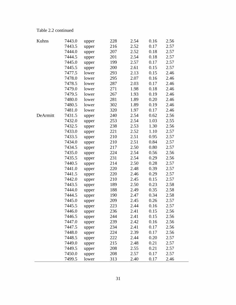
31

Table 2.2 continued

Kuhns 7443.0 upper 228 2.54 0.16 2.56

7443.5 upper 216 2.52 0.17 2.57

7444.0 upper 207 2.52 0.18 2.57

7444.5 upper 201 2.54 0.18 2.57

7445.0 upper 199 2.57 0.17 2.57

7445.5 upper 200 2.61 0.15 2.57

7477.5 lower 293 2.13 0.15 2.46

7478.0 lower 295 2.07 0.16 2.46

7478.5 lower 287 2.03 0.17 2.46

7479.0 lower 271 1.98 0.18 2.46

7479.5 lower 267 1.93 0.19 2.46

7480.0 lower 281 1.89 0.20 2.46

7480.5 lower 302 1.89 0.19 2.46

7481.0 lower 320 1.97 0.17 2.46

DeArmitt 7431.5 upper 240 2.54 0.62 2.56

7432.0 upper 253 2.54 1.03 2.55

7432.5 upper 238 2.53 1.30 2.56

7433.0 upper 221 2.52 1.10 2.57

7433.5 upper 210 2.51 0.95 2.57

7434.0 upper 210 2.51 0.84 2.57

7434.5 upper 217 2.50 0.80 2.57

7435.0 upper 224 2.54 0.56 2.56

7435.5 upper 231 2.54 0.29 2.56

7440.5 upper 214 2.50 0.28 2.57

7441.0 upper 220 2.48 0.39 2.57

7441.5 upper 220 2.46 0.29 2.57

7442.0 upper 210 2.45 0.15 2.57

7443.5 upper 189 2.50 0.23 2.58

7444.0 upper 188 2.49 0.35 2.58

7444.5 upper 190 2.47 0.34 2.58

7445.0 upper 209 2.45 0.26 2.57

7445.5 upper 223 2.44 0.16 2.57

7446.0 upper 236 2.41 0.15 2.56

7446.5 upper 244 2.41 0.15 2.56

7447.0 upper 239 2.42 0.16 2.56

7447.5 upper 234 2.41 0.17 2.56

7448.0 upper 224 2.39 0.17 2.56

7448.5 upper 222 2.44 0.20 2.57

7449.0 upper 215 2.48 0.21 2.57

7449.5 upper 208 2.55 0.21 2.57

7450.0 upper 208 2.57 0.17 2.57

7499.5 lower 313 2.40 0.17 2.46

32

Tab

le 2

.3 M

ean l

og-d

eriv

ed a

ttri

bu

tes

(unco

rrec

ted

) fo

r th

e in

terv

als

of

Mar

cell

us

Shal

e fo

r th

e 1

0

wel

ls a

nal

yze

d.

G

amm

a-ra

y (

AP

I)

B

ulk

-den

sity

(g/c

c)

R

esis

tivit

y (

ohm

-m)

.

Wel

l N

ame

1M

S

Up

Mid

L

ow

M

S

Up

Mid

L

ow

M

S

Up

Mid

L

ow

DeA

rmit

t 284

226

257

385

2.4

9

2.5

1

2.5

0

2.4

5

102

48

101

176

Wei

ster

313

238

278

430

2.4

9

2.5

6

2.4

6

2.4

2

88

42

85

148

Bow

man

300

229

258

427

2.5

1

2.5

7

2.5

1

2.4

2

127

60

132

212

Ger

mro

th

324

234

336

424

2.5

1

2.5

6

2.4

8

2.4

7

101

52

124

146

Spee

r 306

234

271

421

2.4

9

2.5

4

2.4

7

2.4

4

96

68

91

134

Pola

har

306

236

266

420

2.5

2

2.5

6

2.5

2

2.4

8

75

45

69

116

Mounta

in

325

229

344

442

2.4

9

2.5

5

2.4

2

2.4

4

98

54

115

145

Hutc

hin

son

296

235

264

403

2.5

1

2.5

5

2.5

0

2.4

7

84

50

82

130

Kuhns

291

227

264

399

2.5

1

2.5

9

2.5

1

2.3

9

72

40

82

110

Aik

ens

300

231

281

402

2.3

1

2.5

0

2.0

8

2.2

2

82

39

83

136

1M

arce

llus

Shal

e (c

om

pri

ses

the

upper

, m

iddle

, an

d l

ow

er i

nte

rval

s)

33

Table 2.4 Comparison of mean SW values (in decimal) determined from the

modified and standard Archie formulas for the 6 wells having spectral

gamma logs.

SW (mod) SW (std) .

Well Name MS Up Mid Low MS Up Mid Low

Bowman 0.086 0.146 0.076 0.016 0.216 0.283 0.187 0.121

Weister 0.085 0.140 0.074 0.023 0.230 0.317 0.210 0.135

Germroth 0.097 0.163 0.066 0.037 0.230 0.310 0.183 0.164

Speer 0.082 0.122 0.084 0.030 0.210 0.257 0.204 0.156

Polahar 0.098 0.143 0.113 0.031 0.253 0.314 0.251 0.178

Mountain 0.077 0.135 0.048 0.016 0.204 0.278 0.152 0.136

Table 2.5 Mean PHI and TOC predictions using formulas from Core

Laboratories.

PHI TOC (% by wt.) .

Well Name MS Up Mid Low MS Up Mid Low

DeArmitt 0.092 0.082 0.090 0.106 5.5 4.9 5.4 6.4

Weister 0.095 0.075 0.103 0.114 5.7 4.5 6.3 6.6

Bowman 0.089 0.070 0.090 0.114 5.4 4.2 5.4 6.9

Germroth 0.088 0.074 0.095 0.101 5.3 4.5 5.7 6.1

Speer 0.094 0.079 0.099 0.110 5.7 4.7 6.0 6.7

Polahar 0.084 0.073 0.084 0.097 5.1 4.4 5.1 5.9

Mountain 0.096 0.076 0.114 0.109 5.8 4.6 6.9 6.6

Hutchinson 0.088 0.078 0.090 0.099 5.3 4.7 5.5 6.0

Kuhns 0.084 0.066 0.087 0.106 5.1 3.9 5.3 6.5

Aikens 0.089 0.069 0.101 0.113 5.4 4.1 4.1 6.8

Table 2.6 Comparison of core and log-derived parameters at the DeArmitt well.

Core Core Laboratories Archie

Marcellus

Interval

Depth

(ft.) PHI

TOC

(% by wt.) SW PHI

TOC

(% by wt.) SW (std)

Middle 7486.5 0.073 8.0 0.230 0.125 7.6 0.084

Lower 7502.7 0.056 5.2 0.388 0.109 6.6 0.154

Lower 7521.5 0.067 6.3 0.261 0.119 7.3 0.091

34

Figure 2.1 Middle Devonian stratigraphy of southwestern Pennsylvania (modified from

Boyce, 2010). Upper, middle, and lower intervals of the Marcellus Shale are informal

stratigraphic units for the purpose of this study.

A

35

Figure 2.2 Vertical well type log of the Marcellus Shale at the Mamont Prospect.

Boundaries for the Marcellus Shale intervals were picked using the gamma-ray log. The

gamma-ray log is more darkly shaded when 200 API is exceeded. The left side of the log

and the bold lines indicate the boundaries identified for this study. The right side of the

log and the dashed lines indicate boundaries for the stratigraphic nomenclature of the

type area for the Marcellus Shale in New York. (Type log provided by CONSOL Energy)

36

B

Figure 2.3 A= Regional map of study area location within Westmoreland County,

Pennsylvania. B= Local map of the Mamont Prospect showing vertical well locations.

A B A B

A

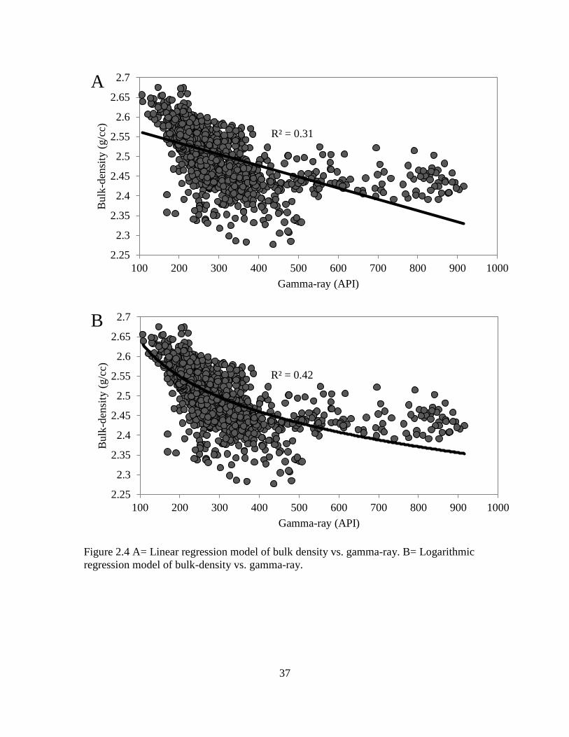
37

R² = 0.31

2.25

2.3

2.35

2.4

2.45

2.5

2.55

2.6

2.65

2.7

100 200 300 400 500 600 700 800 900 1000

Bulk

-den

sity

(g/c

c)

Gamma-ray (API)

R² = 0.42

2.25

2.3

2.35

2.4

2.45

2.5

2.55

2.6

2.65

2.7

100 200 300 400 500 600 700 800 900 1000

Bulk

-den

sity

(g/c

c)

Gamma-ray (API)

Figure 2.4 A= Linear regression model of bulk density vs. gamma-ray. B= Logarithmic

regression model of bulk-density vs. gamma-ray.

B

A

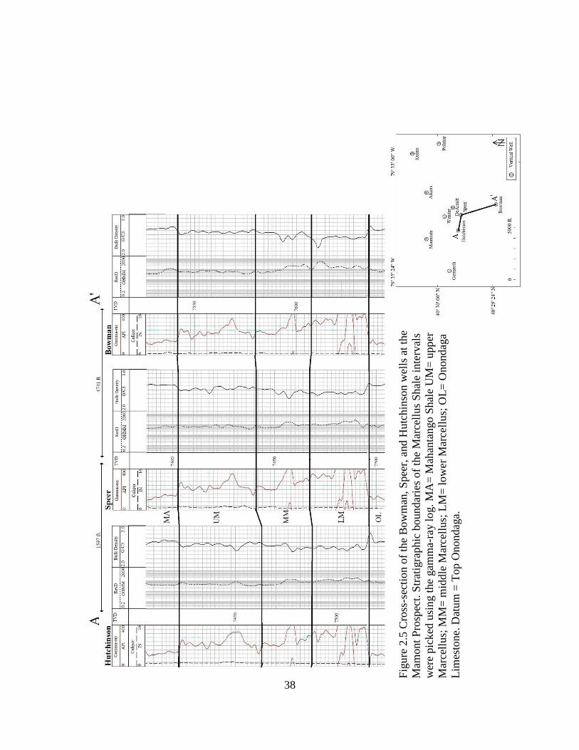
38

Fig

ure

2.5

Cro

ss-s

ecti

on o

f th

e B

ow

man

, S

pee

r, a

nd H

utc

hin

son w

ells

at

the

Mam

ont

Pro

spec

t. S

trat

igra

phic

boundar

ies

of

the

Mar

cell

us

Shal

e in

terv

als

wer

e pic

ked

usi

ng t

he

gam

ma-

ray l

og. M

A=

Mah

anta

ngo S

hal

e U

M=

upp

er

Mar

cell

us;

MM

= m

iddle

Mar

cell

us;

LM

= l

ow

er M

arce

llus;

OL

= O

nondag

a

Lim

esto

ne.

Dat

um

= T

op

Onondag

a.

39

Figure 2.6 Marcellus Shale thickness map. An increase in thickness is observed from the

Germroth well in the west towards the Polahar and Kuhns wells in the east-northeast.

Figure 2.7 Top Marcellus Shale structure map.

40

Figure 2.8 Top Onondaga structure map.

41

2.25

2.3

2.35

2.4

2.45

2.5

2.55

2.6

2.65

2.7

100 200 300 400 500 600 700 800 900 1000

Bulk

-den

sity

(g/c

c)

Gamma-ray (API)

upper middle lower

Linear (upper) Linear (middle) Linear (lower)

Figure 2.9 Regression model displaying the relationship between bulk-density and

gamma-ray for the Marcellus intervals. Data values were obtained from non-rugose

wells. Upper, middle, and lower are references to the Marcellus intervals.

R2

= 0.62

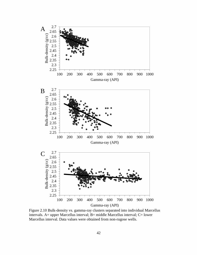
42

2.25

2.3

2.35

2.4

2.45

2.5

2.55

2.6

2.65

2.7

100 200 300 400 500 600 700 800 900 1000

Bulk

-den

sity

(g/c

c)

Gamma-ray (API)

Figure 2.10 Bulk-density vs. gamma-ray clusters separated into individual Marcellus

intervals. A= upper Marcellus interval; B= middle Marcellus interval; C= lower

Marcellus interval. Data values were obtained from non-rugose wells.

2.25

2.3

2.35

2.4

2.45

2.5

2.55

2.6

2.65

2.7

100 200 300 400 500 600 700 800 900 1000

Bulk

-den

sity

(g/c

c)

Gamma-ray (API)

2.25

2.3

2.35

2.4

2.45

2.5

2.55

2.6

2.65

2.7

100 200 300 400 500 600 700 800 900 1000

Bulk

-den

sity

(g/c

c)

Gamma-ray (API)

A

.

B

C

43

Figure 2.11 Isopach map of Marcellus Shale with gamma-ray > 230 API, which has been

recognized (Schmoker 1980) as the threshold between organic-rich and organic-poor

shale.

Figure 2.12 Isopach map of net productive Marcellus Shale, defined by gamma-ray

values >230 API and bulk densities < 2.55 g/cc.

44

Figure 2.13 Iso SW (mod) map of net productive Marcellus Shale. Data points represent

mean SW (mod) calculated for net productive Marcellus Shale.

Figure 2.14 Iso SW (std) map of net productive Marcellus Shale. Data points represent

mean SW (std) calculated for net productive Marcellus Shale.

45

Figure 2.15 Iso-porosity map of net productive Marcellus Shale. Data points represent

mean PHI calculated for net productive Marcellus Shale.

Figure 2.16 Isopach map of net productive Marcellus Shale with TOC greater than 7%.

46

Figure 2.17 Porosity-feet map of net productive Marcellus Shale, defined by mean PHI of

net productive Marcellus Shale * thickness of net productive Marcellus Shale.

Figure 2.18 Isopach map of Marcellus Shale with uranium content > 30 ppm.

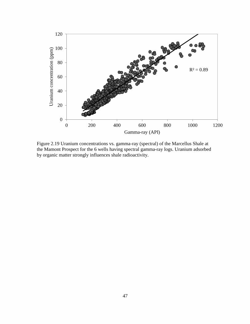
47

R² = 0.89

0

20

40

60

80

100

120

0 200 400 600 800 1000 1200

Ura

niu

m c

on

centr

atio

n (

pp

m)

Gamma-ray (API)

Figure 2.19 Uranium concentrations vs. gamma-ray (spectral) of the Marcellus Shale at

the Mamont Prospect for the 6 wells having spectral gamma-ray logs. Uranium adsorbed

by organic matter strongly influences shale radioactivity.

48

CHAPTER THREE: CHAPTER THREE: HORIZONTAL WELL

INVESTIGATION: ASSESSMENT OF THE RELATIONSHIPS AMONG

MUD-LOGGING GAS, WELL DESIGN, AND PRODUCTION IN THE

MARCELLUS SHALE

3.1 Abstract

To assess the resource potential of the Marcellus Shale within the Mamont

Prospect in Westmoreland County, Pennsylvania, gamma-ray, penetration (minutes per

foot drilled), and mud-logging gas (total gas) from 12 horizontal wells were examined.

Total gas was evaluated as a shale-gas resource per unit volume of hole drilled. Well

design parameters, which include lateral length, number of fracture stages, and sand per

fracture stage, were examined to understand their influence on cumulative production.

Values of mean gamma-ray and mean penetration for 3 intervals of Marcellus

Shale indicate increasing organic matter content in stratigraphically descending intervals.

Total gas calibrated for gas trap performance (TGTRAP) and total gas calibrated for

penetration and hole-size (TGPH) correlate with cumulative production (R2=0.87 and

R2=0.70, respectively). TGTRAP and TGPH per lateral-ft also show correspondence with

cumulative production per lateral-ft (R2=0.52 and R

2=0.40, respectively). Cumulative

production increases approximately 215 million cubic feet for every 1000 feet of lateral

length and approximately 256 million cubic feet for every 4 fracture stages. Sand per

fracture stage shows no correspondence with production. This investigation is unique in

using mud-logging gas as an indicator of well performance for horizontal wells

completed in a shale-gas reservoir.

49

3.2 Introduction

Although shale-gas reservoir development is a growing source of natural gas

reserves, great uncertainties exist regarding recovery of natural gas from unconventional

reservoirs. Challenges include effective methods of drilling, completions, and stimulation

(Lee et al., 2011). Over the last several years, increased interest in low-permeability

formations has required fine-tuning of existing methodologies to predict parameters that

are essential for evaluation of shale-gas reservoirs, such as the Marcellus Shale of the

Appalachian Basin (Boyce, 2010). A universal practice has been to relate well-log

measurements to rock properties, providing both qualitative and quantitative assessments

of reservoir potential. More recently, however, a number of studies have looked to well

planning, drilling operations, and production as a means to assess well performance. This

study, an assessment of the Mamont Prospect in Westmoreland County, Pennsylvania,

focuses on mud-logging gas and its efficacy as a predictor of well performance within the

Marcellus Shale. The ultimate yield of natural gas from the Marcellus Shale is estimated

to be 489 trillion cubic feet (Engelder, 2009; Pifer, 2010).

In Devonian shales, organic matter is the source of the large quantities of natural

gas (Schmoker, 1981). At a given location, the amount of organic matter correlates

approximately with the volume of producible gas in the shale matrix (Schmoker, 1981).

Laboratory analyses provide a means to directly quantify organic matter, a measurement

expressed as total organic carbon (TOC). In New York, TOC for the Marcellus Shale

increases westward from central to western New York, where maximum values approach

6% (Hill et al., 2004). From New York southward to West Virginia a general decrease in

TOC is observed (Milici and Swezey, 2006). Repetski et al. (2002) determined TOC to

50

be 3 to 6% in east-central Pennsylvania. The basal part of the Marcellus Shale in West

Virginia yields 8.8% maximum TOC and 5.2% mean TOC (Zielinski and Nance, 1979).

Efforts to produce natural gas currently involve both vertical and horizontal

drilling (Lee et al., 2011). Recent industry practices, however, favor horizontal drilling,

as the total drainage of traditional, vertical wells is much smaller than the total drainage

of horizontal wells in the same target zone (Larch, 2012). Measurement while drilling

(MWD) is standard procedure during horizontal drilling to record tool position, tool

orientation, and formation parameters along the wellbore. Tools implementing MWD are

referred to as logging while drilling (LWD) tools, and are used during the drilling of

horizontal wells to keep the drill-bit inside a thin reservoir (geo-steering). The

predominant method for geo-steering in shales is using natural gamma-ray LWD tools,

which measure naturally occurring gamma radiation (i.e., thorium, potassium, and

uranium) emitted from the formation (Pitcher and Jackson, 2012). Gamma-ray

measurement provides a qualitative view of the rock, such as shale or shaleyness, and

limestone or marl (Pitcher and Jackson, 2012). Gamma-ray is an effective tool because of

its relationship with organic matter (Schmoker, 1980; Schmoker, 1981; Sondergeld et al.,

2010), providing a simple approach for TOC approximation.

For decades, before the advent of LWD tools, indications of reservoir potential

were procured from the mud-log (Ablard et al., 2012). Mud-logging is standard

procedure during drilling and involves the collecting of both qualitative and semi-

quantitative data from hydrocarbon gas detectors (Crain, 2008). As the drill bit

disaggregates the rock, gas and other components present in the pore space enter the

drilling fluid (mud) (Erzinger et al., 2006). Hydrocarbons are then conveyed to the

51

surface in two forms: 1) produced into the mud; and 2) retained by cuttings (Mercer,

1974). Gas traps at the surface allow for the gas to be sampled for total gas (TG) and

chromatographic analysis. Detected components are typically within the alkane group:

methane, ethane, propane, butane, and pentane (Ablard et al., 2012). The sum of these

components is denoted as TG, and is generally used to determine if an oil or gas reservoir

has been penetrated (Crain, 2008). Results are typically expressed in parts per million

(ppm) of equivalent methane in air (EMA), where 1% methane is equivalent to 10,000

ppm (Ablard et al., 2012). Common practice has been to re-label these units as gas units,

where 1% EMA is equivalent to 50 gas units (Whittaker, 1987).

For safety purposes, mud-logging aims to detect over-pressured zones and lost

circulation. For reservoir evaluation, the purpose of mud-logging is to identify all

hydrocarbon indicators from the oil and gas trapped in the drilling fluid (Crain, 2008).

Mud-retained gases comprise 5 components: recycled gas, trip gas, produced gas,

contamination gas, and liberated gas (Mercer, 1974). Liberated gas, which is the gas

mechanically released into the drilling fluid as the drill-bit disaggregates the rock

formation (Mercer, 1974), is the only component indicative of a potential prospect

(Crain, 2008). Contributing to gas liberation are 3 factors: penetration (i.e., time per unit

depth of drill bit; min/ft), porosity, and formation pressure (Mercer, 1974). Williams and

Ewing (1989) noted variations in gas response from changes in gas trap design, which

include trap position, the presence or absence of a bottom lip, mud levels, and air

sparging. According to Donovan (2007), the primary, deterministic factors influencing

gas response are penetration, pump rate, and hole-size. Other factors include background

gas and surface losses (Donovan, 2007).

52

Due to the number of factors influencing gas measurement during drilling,

quantitative analyses of mud-logging gas have widely been rejected. Published studies

using mud-logging gas are scarce and have largely focused on coal-bed methane (CBM)

wells. In a study by Donovan (2003), that included 55 CBM wells in the Powder River

Basin, gas content was estimated from mud-logging gas and 2.5 years cumulative

production. It was concluded that mud-logging gas, when properly calibrated, can be

used as a predictive tool to assess future performance of wells completed in

unconventional reservoirs. Factors influencing the gas response of the mud-logging unit

were accounted for using a calibration method known as carbide lagging (Donovan,

2003). Carbide lags were not employed during drilling operations for wells in this study.

Relationships among well design, reservoir characteristics, and production have

been studied by numerous researchers to understand their influence on performance of

Devonian shale wells (Gatens et al., 1989; Schweitzer, 2009; Larch, 2012). From 26

horizontal Marcellus Shale wells scattered throughout Pennsylvania and West Virginia,

Larch (2012) found no correlation between the number or length of fracture stages and 2

years production. Schweitzer (2009) determined that as wellbore length increases, gas

production increases approximately 250 million cubic feet (MMCF) per 1000 feet of

wellbore. In a study of more than 800 eastern Devonian shale vertical wells, Gatens et al.

(1989) developed analytical tools to predict future production from permeability-

thickness product and estimations of gas-in-place. No studies were found, however, that

assessed relationships among mud-logging gas parameters and production for Marcellus

Shale horizontal wells. Therefore, the primary objectives of this research are: 1) assess

shale-gas resource potential of the Marcellus Shale using LWD and mud-logging

53

parameters; 2) determine if mud-logging gas can be used as an indicator for shale-gas

resource per unit volume of hole drilled; and 3) determine the influence of well design

parameters on cumulative production. Well design parameters include lateral length (LL),

number of fracture stages, and sand per fracture stage.

3.3 Geologic Setting

The Appalachian Basin is a northeast-southwest trending foreland basin that

formed during the Middle to Late Ordovician Taconic orogeny (Faill, 1997). During the

Acadian Orogeny (Middle Devonian), basin filling was dominated initially by organic-

rich black shale, a consequence of paleoclimatic and paleogeographic constraints

(Ettensohn, 1987). The author proposed that deposition of black shale occurred when

basins were deepest, most restricted, and received least sediment. Deep, anoxic

conditions represented by the shale and the sharp contact between basal units suggest the

basins were formed during periods of abrupt subsidence (Ettensohn, 1987). Schwietering

(1981) proposed that black shale was deposited in an epeiric sea of a shallow basin,

allowing for the preservation of organic material through anaerobic conditions.

Comprised of two black shale units separated by intercalated limestone, shale, and

sandstone, the Middle Devonian Marcellus Shale Formation occurs in the basal Hamilton

Group, an east to southeastward thickening succession of marine and non-marine shale,

siltstone, and sandstone (Lash and Engelder, 2011). The Marcellus Shale in New York

(i.e., the type area for the Marcellus Shale) comprises, in stratigraphically ascending

order, the Union Springs, Cherry Valley, and Oatka Creek members. The Union Springs

Member is a radioactive, low-density shale directly above the Onondaga Formation (Lash

and Engelder, 2011). The Cherry Valley Member consists of nodular limestone, shale,

54

and siltstone, and is recognized by low radioactivity (Lash and Engelder, 2011). The

Oatka Creek Member is recognized by a radioactive basal section and a less radioactive,

higher density upper section (Lash and Engelder, 2011). In southwestern Pennsylvania,

the Oatka Creek and Union Springs members are typically referred to as the Upper and

Lower Marcellus Shale members and are separated by the Purcell Limestone, a

correlative of the Cherry Valley Member (Lash and Engelder, 2011). For this

investigation, three informal stratigraphic intervals (i.e., upper, middle, and lower) of the

Marcellus Shale were defined (Figure 3.1).

Extending from Ohio to Pennsylvania, the Marcellus Shale varies from 50 to 200

feet in thickness and occurs 1,000 to 7,000 feet below the top of Devonian strata (Soeder,

2010). The Marcellus Shale is predominantly gray-black to black, thinly laminated, non-

calcareous, and fissile (Boyce, 2010). Analyses of core samples by x-ray diffraction

revealed high quartz content (60%), low clay content (30%), and pyrite (10%) (Boyce,

2010).

Within the Mamont Prospect the Marcellus Shale overlies limestone of the

Middle Devonian Onondaga Formation and underlies the Middle Devonian Mahantango

Shale, a mix of mudstone, sandstone, limestone, and conglomerate (Bruner and Smosna,

2011). The Mamont Prospect contains 10 vertical and 13 horizontal gas-producing wells

within an area of 9 square miles (Figure 3.2).

3.4 Methods

3.4.1 Shale Gas Resource Potential Using LWD and Mud-logging Parameters

Shale-gas resource potential was assessed using the following mud-logging

parameters: penetration and TG. LWD gamma-ray was also used. This assessment was

55

accomplished by: 1) obtaining mud-logs and completion reports from CONSOL Energy;

2) identifying stratigraphic boundaries for the Marcellus Shale intervals; 3) ensuring

accuracy of Marcellus Shale correlations; 4) generating histograms of mean gamma-ray

and mean penetration; and 5) assessing the relationship between LWD and wireline

gamma-ray logs.

3.4.1.1 Data Collection and Preparation

The drilling of 13 horizontal wells targeting the Marcellus Shale was directed by

CONSOL Energy. LAS (Log ASCII Standard) files containing depths, geophysical logs,

mud-gas logs, and other well parameters were produced and updated throughout drilling

operations. Measurements of gamma-ray, penetration, and mud-logging gas (i.e., TG, C1,

C2, C3, and C4) were recorded in 1-foot increments. After well drilling, LAS files were

imported into GeoGraphix® software. For calculation purposes, LAS files were imported

into Microsoft Excel. A mud-log LAS file for DeArmitt 1B was not available.

3.4.1.2 Stratigraphic Boundaries of the Marcellus Intervals

In XSection, a GeoGraphix®

module, stratigraphic tops were ‘picked’ at gamma-

ray inflection points for the Onondaga Limestone and the 3 intervals of Marcellus Shale

(Figure 3.3). From the 10 vertical wells at the Mamont Prospect, a 10 well cross-section

was created and used as reference to maintain consistency in picks from well-to-well. A

zone of low gamma radiation, ranging from 2 to 16 ft. in thickness, separates each

Marcellus Shale interval. Top of the upper Marcellus was picked at the base of the

Mahantango Shale beneath a pronounced shelf of gamma radiation below 160 API.

Similarly, the top of the Onondaga Limestone was picked at the top of a pronounced shelf

of gamma radiation below 160 API. Top of the middle and top of the lower Marcellus

56

intervals were each picked at the base of a decreased gamma-ray response directly below

a gamma-ray kick (i.e., a gamma-ray deflection to the right). Among the 10 vertical

wells, gamma-ray values peak at 320 to 360 API for the upper Marcellus, 440 to 480 API

for the middle Marcellus, and 700 to 760 API for the lower Marcellus.

3.4.1.3 Marcellus Shale Correlations

For the 12 wells studied, 3D models of the Onondaga Limestone and the 3

Marcellus intervals were built in GeoGraphix® by CONSOL Energy using geo-steering

techniques. While geo-steering, correlations were made along the wellbore path using the

LWD gamma-ray log. By assuming constant thickness of formation intervals,

correlations were added along the wellbore path by inserting tie lines from the gamma-

ray logs of neighboring vertical well picks, or recent inter-well picks, to correlative points

on the gamma-ray logs of current inter-well sections. As the inclinations of the wells

changed relative to the bedding dip angles, gamma-ray logs were stretched, compressed,

or flipped to make correlations.

Accuracy of the correlations displayed is a function of the number of data points

present in the model. For the 12 horizontal wells in this study, inter-well correlations

were added to each geo-steering model by inserting tie lines from the gamma-ray logs of

inter-well picks (i.e., correlations previously made by CONSOL Energy) to correlative

points on the gamma-ray logs of additional inter-well sections. By adding inter-well

correlations, tops for the Onondaga Limestone and the 3 Marcellus intervals were

projected more accurately across the geo-steering model. Single well diagrams displaying

wellbore path and interval tops for the Onondaga Limestone and the 3 Marcellus intervals

were produced (Figures A.6-A.17).

57

3.4.1.4 Histograms of Gamma Radiation and Penetration

For the 12 horizontal wells, gamma radiation and penetration were compared

among the 3 Marcellus intervals. Single well diagrams (Figures A.6-A.17) were used to

assign data values (i.e., measurements of gamma-ray and penetration) to Marcellus

intervals along each lateral length (LL) (i.e., wellbore section designated for hydraulic

fracture treatment). After assigning data values from LAS files to Marcellus intervals,

values of mean penetration and mean gamma-ray were calculated for each Marcellus

interval to produce histograms for each of the 12 wells. Histograms were used to assess

changes in gamma radiation and penetration with depth.

3.4.1.5 LWD and Wire-line Gamma-ray Relationship

Discrepancies between LWD and wire-line gamma-ray logging, which is done

after drilling, have been recognized in previous studies (e.g., Mendoza, 2006). To assess

the relationship between LWD gamma-ray and wire-line gamma-ray at the Mamont

Prospect, and to define a boundary for shale of high gas content for LWD gamma-ray, a

complex depth shift was performed using GeoGraphix®; a technique used to

stratigraphically align geophysical logs for comparison. Wells were selected using the

following criteria: 1) must have good representation of the Marcellus Shale (i.e.,

completely penetrate all Marcellus intervals); 2) vertical and horizontal wells must be

within a 1000 ft. radius of one another (to help disclaim lateral heterogeneity); and 3)

have a complete set of gamma-ray measurement. The Hutchinson 4G and DeArmitt 1A

horizontal wells and the Mountain and Speer vertical wells met these criteria. By

exporting and saving total-vertical-depth (TVD) values, LWD gamma-ray logs were

displayed vertically for the 2 horizontal wells. LWD and wire-line gamma-ray logs were

58

then stratigraphically aligned by adding tie lines to correlative points from each gamma-

ray log (Figure 3.4).

Schmoker (1980) proposed that a boundary (i.e., 2% organic content by volume)

between organic-rich and organic-poor shale exists at 230 API and that this value

represents a threshold for shale of high gas content. Furthermore, 2% organic content by

volume is a commonly accepted division between hydrocarbon source and non-source

rocks (Schmoker, 1980). This boundary is based entirely on interpretation from wireline

gamma-ray logs. To identify a best-fit equation to estimate LWD gamma-ray

corresponding to 230 API (wire-line gamma-ray), LWD and wire-line gamma-ray values

were cross-plotted in GeoGraphix®

. The LWD gamma-ray value corresponding to 230

API wire-line was used to define the boundary between organic-rich and organic-poor

shale based on LWD gamma-ray. This boundary was applied to interpreting if each of the

3 Marcellus intervals contained high gas content or low gas content.

3.4.2 Mud-Logging Gas as an Indicator of Shale-Gas Resource per Volume of Hole

Drilled

Mud-logging TG was assessed by 1) calibrating TG measurements to account for

changes in gas trap/mud-logging gas sampler performance; and 2) expressing TG as a

resource per unit volume of hole drilled. Production data are based on 18 months

cumulative and were obtained from CONSOL Energy. Cumulative production was used

in this investigation because the independent variable (production) in most statistical

studies is assumed to have no error. Estimated ultimate recovery (EUR) is a forecast, and

therefore has the potential of having indeterminate error. A correlation between

cumulative production and EUR was performed to demonstrate the uncertainty in

59

forecasting EUR (Figure A.18). EUR data obtained from CONSOL Energy were based

on 6 months production.

3.4.2.1 Calibrating TG to Account for Gas Sampler Performance

Large variations in performance exist among gas traps and sampling systems as a

result of operational and design factors (Williams and Ewing, 1989). In most instances,

the mud-logging unit gas, total gas sensors, and chromatograph are calibrated, but the

total mud-logging sampling system is not (William Donovan, personal communication).

Two types of calibrations are typically performed. One calibration is known as “zeroing,”

which is equivalent to adjusting the intercept of a y = mx + b linear equation, and the

second is span adjustment, which is equivalent to changing the slope of a linear equation

(William Donovan, personal communication). Two points were measured for each of the

12 horizontal wells. The first point was air, which assumed a zero reading. The second

point was mean TG in the basal part of the Mahantango Shale, a section having consistent

geophysical log readings (i.e., gamma-ray ranging from 120 to 125 API) across the study

area. Using TG measurements from LAS files, a mean TG was calculated for the basal

part of the Mahantango Shale (i.e., the 50 ft. measured depth (MD) up-section from the

Marcellus-Mahantango Shale contact). Additive (zeroing) factors, analogous to the

amount of deviation away from 350 gas units (i.e., Mahantango Shale mean TG from 350

gas units), were applied to Marcellus Shale TG measurements on a foot-by-foot basis.

350 gas units represent an arbitrary TG value assumed for typical gas trap/sampling

system performance in the Mahantango Shale. TG calibration on the Mahantango Shale

can be observed in Figure 3.5. TGTRAP measurements (i.e., TG calibrated for gas

trap/sampling performance) were summed along each well’s LL and cross-plotted against

60

cumulative production. TGTRAP was evaluated on a per lateral-ft basis by cross-plotting

TGTRAP per lateral-ft (i.e., sum of measurements along LL divided by LL) against

cumulative production per lateral-ft (i.e., cumulative production divided by LL) for each

of the 12 wells.

3.4.2.2 Total Gas as a Unit Volume

Penetration, mud pump rate, and hole size are the primary factors influencing

mud-logging gas response, according to Donovan (2007). With all other factors equal,

halving penetration (i.e., doubling drilling rate) doubles the gas show, doubling mud

pump rate halves the gas show, and doubling hole-diameter quadruples the gas show

(Donovan, 2007; Walsh and Donovan, 2007). For the 12 wells studied, pump rates were

recorded as daily averages, and are therefore insufficient to include in this investigation.

Average daily pump rates were consistent, however, ranging from 425 to 445 gallons per

minute (GPM). To account for variations in gas response due to penetration and hole-

size, a calibrated TG was computed using Equation 1 (William Donovan, personal

communication).

TGPH = P*(1/AWB)*TG Equation 1

where TGPH is TG calibrated for penetration and hole size (gas units x min/ft3); P is

penetration (min/ft); AWB is wellbore cross-sectional area (ft2) determined from tool bit-

size; and TG is total gas (gas units). TGPH represents the amount of gas liberated per

volume of hole drilled for a unit time. As gas liberation is attributed largely to penetration

(Mercer, 1974), the units of TGPH are appropriate. For each of the 12 wells, Equation 1

was applied on a foot-by-foot basis. To account for gas sampling system performance, as

similar to TGTRAP calibration, a zeroing adjustment was performed on the basal part of

61

the Mahantango Shale. TGPH measurements were calibrated to 1500 gas units x min/ft3, a

value assumed for typical gas sampling performance. TGPH measurements were summed

along each well’s LL and cross-plotted against cumulative production. TGPH per lateral-ft

was cross-plotted against cumulative production per lateral-ft.

3.4.3 Assessing Influence of Well Design Parameters on Formation Drainage

Volume

To assess the influence of well design on formation drainage volume, parameters

including LL, number of fracture stages, and total proppant (sand) were cross-plotted

against cumulative production for each of the 12 wells. To determine whether production

is interval-dependent or high-gamma-ray-dependent (i.e., regardless of interval), gamma-

ray sum (i.e., sum of gamma-ray along LL) was cross-plotted against cumulative

production. Gamma-ray per lateral-ft was cross-plotted against cumulative production per

lateral-ft. The number of lateral feet in the middle interval (i.e., along LL) was divided by

total LL and cross-plotted against cumulative production per lateral-ft. This step was

repeated for the lower interval.

3.5 Results

3.5.1 Shale Gas Resource Potential Using LWD and Mud-logging Parameters

3.5.1.1 Data Collection and Preparation

From drilling and completion reports, total depths (TD) for the 12 horizontal

wells range from 10,100 to 13,545ft (Table 3.1). LLs range from 2,154 to 5,324 ft (Table

3.2).

62

3.5.1.2 Stratigraphic Boundaries of the Marcellus Intervals

Stratigraphic boundaries, defined in cross-section using gamma-ray logs from 10

vertical wells, reveals that Marcellus Shale thickness ranges from 88.5 to 98 ft (Table

3.1). The upper Marcellus is the thickest interval ranging from 37.1 to 44 ft.

3.5.1.3 Marcellus Shale Correlations

Geo-steering efforts and the added inter-well correlations reveal that 46,778 total

feet of wellbore among the 12 wells studied traverse the Marcellus Shale. Of the total

feet, 5% are in the upper interval, 50% are in the middle interval, and 45% are in the

lower interval. All 12 wells penetrate completely through the upper interval and at least

half-way through the middle interval.

3.5.1.4 Histograms of Gamma Radiation and Penetration

Estimated from the 12 wells studied, mean gamma-ray and mean penetration for

the Marcellus intervals in stratigraphically descending order are 182, 217, and 242 API,

respectively; and 1.3, 0.78, and 0.63 min/ft., respectively. For the majority of wells (11 of

12), mean gamma-ray increases in stratigraphically descending Marcellus intervals

(Figure 3.6 A). For the majority of wells (9 of 12), mean penetration decreases in

stratigraphically descending Marcellus intervals (Figure 3.6 B).

3.5.1.5 LWD and Wire-line Gamma-ray Relationship

A trend-line was fit to LWD gamma-ray and wire-line gamma-ray data values

yielding an R2 of 0.83 (Figure 3.7). Wire-line gamma-ray and LWD gamma-ray values

range from 62 to 897 API and 62 to 562 API, respectively. From a power equation

(Equation 2), determined from the trend-line in Figure 3.7, the threshold for shale of high

63

gas content corresponding to 230 API wireline gamma-ray is 205 API for the LWD

gamma-ray:

y = 0.11046 x1.435

Equation 2

where y is wireline gamma-ray (API) and x is LWD gamma-ray (API). Mean gamma-ray

is above this threshold for the middle and lower Marcellus intervals (217 and 242 API,

respectively) and below for the upper Marcellus interval (187 API).

3.5.2 Mud-Logging Gas as an Indicator of Shale-Gas Resource per Volume of Hole

Drilled

3.5.2.1 Calibrating TG to Account for Gas Sampler Performance

The summation of TGTRAP along LL correlates with cumulative production

(R2=0.86) (Figure 3.8 A). TGTRAP per lateral-ft also correlates with cumulative

production per lateral-ft (R2=0.52) (Figure 3.8 B).

3.5.2.2 Total Gas as a Unit Volume

The summation of TGPH along LL shows correspondence with cumulative

production (R2=0.70) (Figure 3.9 A). TGPH per lateral-ft shows moderate correspondence

with cumulative production per lateral-ft (R2=0.40) (Figure 3.9 B).

3.5.3 Influence of Completion Variables on Formation Drainage Volume

LL and number of fracture stages correlate with cumulative production (R2=0.74

and R2=0.74) (Figures 3.10 A and B). Similar R

2 values for these design parameters were

anticipated as the number of fracture stages is typically dependent on LL. For every 1000

feet of wellbore cumulative production increases approximately 215,000 MCF (thousand

cubic feet). For every 4 fracture stages, cumulative production increases approximately

256,000 MCF. Cumulative production per fracture stage shows no correlation with sand

64

per fracture stage (Figures 3.11). Gamma-ray sum has as strong correlation with

cumulative production (Figure 3.12 A). Correlation between gamma-radiation per lateral-

ft and cumulative production per lateral-ft is weak (R2=0.24) (Figure 3.12 B). Cross-

plots of cumulative production per lateral-ft against total lateral feet in upper interval and

total lateral feet in lower interval reveal R2 values of 0.18 and 0.80, respectively (Figures

3.13 A and B). Cumulative production for wells with more than 80% of their total lateral

feet in the middle interval ranges from 177 to 385 MCF per lateral-ft (Figure 3.13 A).

Cumulative production for wells with more than 80% of their total lateral feet in the

lower interval ranges from 300 to 355 MCF per lateral-ft (Figure 3.13 B).

3.6 Discussion

Correlation between organic matter content and gamma-ray within Devonian

shales reflects the association of uranium with organic matter (Schmoker, 1981). This

relationship likely exists because uranium is easily adsorbed by carbonaceous material, a

result of hexavalent uranium (U+6

) reducing to U+4

(Fertl and Chilingar, 1988). For the

majority of wells (11 of 12), mean gamma-ray increases in stratigraphically descending

Marcellus intervals (Figure 3.6 A) indicating increased organic matter content with depth.

Calculated from all 12 wells, mean gamma-ray values in stratigraphically descending

Marcellus intervals are 182, 217, and 242 API, respectively.

During shale-gas resource assessment, particular emphasis has been placed on

identifying over-pressured areas (i.e., where pore pressure exceeds hydrostatic pressure).

Chaney (1950) postulated that over-pressure may be the result of oil or gas cracking

within the reservoir. The volume increase from gas generation can be very large where

organic matter is cracked to gas (Hedberg, 1974). Luo and Vasseur (1996) showed that

65

below a certain depth, oil to gas cracking can have a large influence on over-pressure

mechanisms, which becomes more important as organic matter content increases.

Moreover, Jorden and Shirley (1966) postulated that a plot of drilling rate (i.e., inverse of

penetration) versus depth should define an ever-decreasing trend in the normal pressure

section, and a trend reversal (i.e., increasing trend) in the over-pressured section. For the

majority of wells (9 of 12) mean drilling rates increase in stratigraphically descending

Marcellus intervals (Figure 3.6 B), indicating increasing organic matter content and

possibly greater overpressure with depth.

Donovan (2003) demonstrated that gas response obtained from the mud-logging

unit can be calibrated and used as an indicator of well performance for unconventional

CBM wells. He found that gas content estimated from mud-logging gas was more

predictive than gas content estimated from core desorption isotherm data. For the 12

wells in this study, calibrated mud-logging gas (TGPH) shows correspondence with

cumulative production (Figures 3.8 and 3.9). While Donovan (2003) used carbide lags to

calibrate the gas response and an intermediate step to calculate gas content this study

used the Mahantango Shale to calibrate the gas response and an intermediate step to

calculate the amount of gas liberated per volume of hole drilled per unit time. The results

from both studies reveal that mud-logging gas (i.e., when properly calibrated) can be used

as an indicator of well performance in unconventional reservoirs. This is the only known

study using mud-logging gas as an indicator of well performance in a shale-gas reservoir.

Total organic carbon (TOC) and its overall control on gas accumulation in shales

(Ding, 2011) is important in understanding the effectiveness of mud-logging gas in

indicating performance of horizontal wells completed in the Marcellus Shale. Where

66

contents of organic matter and quartz are high, increased brittleness, decreased tensile

strength, and increased proneness to fracturing has been observed; such properties favor

shale-gas desorption, free gas accumulation, and flow (Ding et al., 2012).

Ita (2011) modeled the impact of well design on cumulative production using

input parameters representative of numerous Devonian shale units (i.e., Barnett, Ohio,

Fayetteville, etc.) and found that cumulative production increases approximately 200,000

MCF for every 1000 feet of lateral well length. Using input parameters specific to the

Marcellus Shale, Schweitzer (2009) observed a 250,000 MCF increase in cumulative

production for every 1000 feet of lateral well length. Similarly, for the 12 horizontal

wells in this study, cumulative production increases approximately 215,000 MCF for

every 1000 feet of lateral well length (Figure 3.10 A).

Schweitzer (2009) and Larch (2012) observed an increase in production with an

increase in the number of fracture stages. Similarly, for the 12 wells in this study,

correlation between the number of fracture stages and cumulative production was

observed (R2 = 0.74) (Figure 3.10 B). Larch (2012) found no correlation between

proppant (sand) per fracture stage and cumulative production, and for the 12 wells in this

study, weight of sand per fracture stage did not correlate with cumulative production per

fracture stage (Figure 3.11).

Figures 3.12 and 3.13 indicate that production from the Marcellus Shale may be

largely zone-dependent, rather than high-gamma-ray-dependent. Cumulative production

per lateral-ft. versus gamma-ray per lateral-ft. yields an R2 of 0.24; with the most

productive well (Hutchinson 4J) having the second lowest gamma-ray per lateral-ft. (210

API). Completing horizontal wells in the lower Marcellus interval shows the best

67

correlation with production per lateral-ft (R2=80) (Figure 3.13 B) compared with

horizontal wells completed in the middle Marcellus interval (R2=0.18) (Figure 3.13 A).

Completing horizontal wells in the middle Marcellus interval may be risky, as production

per lateral-ft varies by nearly 200 MCF per lateral-ft (i.e., for LLs having 80% or more

total feet in the middle interval).

3.7 Conclusion

Mean values of gamma-ray and penetration measured along LL for the 3 intervals

of Marcellus Shale indicate increasing organic matter content in stratigraphically

descending intervals. A complex depth shift reveals an R2 of 0.83 between wireline

gamma-ray and LWD gamma-ray. The boundary between organic-poor and organic-rich

shale exists at 205 API for LWD gamma-ray, indicating that the upper Marcellus interval

(187 API mean) falls beneath the threshold for shale of high gas content. Calibrated TG

measurements (i.e., TGTRAP and TGPH) show correspondence with cumulative production

(R2=0.87 and R

2=0.70, respectively). Although weaker correlation coefficients were

observed, TGTRAP and TGPH measurements (i.e., on a per lateral-ft. basis) showed

correspondence with cumulative production per lateral-ft (R2=0.52 and R

2=0.40,

respectively). Well design parameters, which include LL and number of fracture stages,

correlate with cumulative production (R2=0.74 and R

2=0.74, respectively). For every

1000 feet of LL, production increases approximately 215,000 MCF. The correlation

between percent of LL in the lower Marcellus and cumulative production per lateral-ft

(R2=0.80) indicates that the lower Marcellus contributes more to cumulative production

than the middle Marcellus interval. This study provides a simple methodology (i.e.,

calibrating TG on the Mahantango Shale and expressing TG as a volume of liberated gas

68

per unit volume of hole drilled) to effectively use mud-logging gas as an indicator of

performance for horizontal wells completed in the Marcellus Shale. This method is

sufficiently straightforward to be used in real-time during drilling operations.

3.8 References

Ablard, P., Bell, C., Cook, D., Fornasier, I., Poyet, J., Sharma, S., Fielding, K., Lawton,

L., Haines, G., McCarthy, K., Radakovic, M. & Umar, L. (2012). The Expanding

Role of Mud Logging, Oilfield Review, 24(1), 24-41.

Adamson, K., Birch, G., Gao, E., Hand, S., Macdonald, C., Mack, D. & Quadri, A.

(1998). High Pressure, High Temperature Well Construction, Oilfield Review

10(2), 36-49.

Amen, R. M. (1994). Quantifying Hydrocarbon Shows Using On-Line Gas

Referencing. SPWLA 35th Annual Logging Symposium, Tulsa, Oklahoma, 19-22

June, 1994.

Boyce M. L. (2010). Sub-surface Stratigraphy and Petrophysical Analysis of the Middle

Devonian Interval of the Central Appalachian Basin; West Virginia and

Southwest Pennsylvania, PhD Dissertation, West Virginia University.

Chaney, P. E. (1950). Abnormal pressure and lost circulation: World Oil, 130, 122-

126.

Cook, T. (2003). Calculation of Estimated Ultimate Recovery (EUR) for Wells in

Continuous-Type Oil and Gas Accumulations of the Uinta-Piceance Province.

International Journal of Coal Geology 56, 39-44.

Crain, E. R. (2002). Crain’s petrophysical handbook. Available at:

http://www.spec2000.net. Sugar Land, Texas: Schlumberger.

Ding, W., Li, C., Li, C., Xu, C., Jiu, K., Zeng, W. & Wu, L. (2012). Fracture

development in shale and its relationship to gas accumulation. Geoscience

Frontiers, 3(1), 97-105.

Donovan, W. (2000). Mudlogging method calculates coalbed gas content. Oil & Gas

Journal, 98(7), 64.

Donovan, W. (2003). Mudlogging Gas Content Results Compared to Production

Performance. PowerPoint presented at Society of Petroleum Engineers (SPE)

Luncheon Program, Denver, Colorado, 17 December.

69

Donovan, W. (2007). Mudlogging Unconventional Gas Reservoirs. PowerPoint presented

at Unconventional Gas Technical Forum, Victoria, British Columbia, Canada,

Ministry of Energy, Mines and Petroleum Resources, 16 April.

Engelder, T. & Lash, G.G. (2008). Marcellus Shale play’s vast resource potential

creating stir in Appalachia. The American Oil and Gas Reporter, 7 pp., May.

Engelder, T. (2009). Marcellus 2008: Report card on the breakout year for gas production

in the Appalachian Basin. Fort Worth Basin Oil and Gas Magazine, 20, 18-22.

Erzinger, J., Wiersberg, T. & Zimmer, M. (2006). Real-time mud gas logging and

sampling during drilling, Geofluids, 6(3), 225-233.

Ettensohn, F. R. (1987). Rates of relative plate motion during the Acadian orogeny based

on the spatial distribution of black shales. The Journal of Geology, 95(4), 572-

582.

Faill, R. T. (1997). A geologic history of the north-central Appalachians; Part 1,

Orogenesis from the Mesoproterozoic through the Taconic Orogeny. American

Journal of Science, 297(6), 551-619.

Gatens III, J. M., Lee, W. J., Lane, H. S., Watson, A. T., Stanley, D. K. & Lancaster, D.

E. (1989). Analysis of eastern Devonian gas shales production data. Journal of

Petroleum Technology, 41(5), 519-525.

Hedberg, H. D. (1974). Relation of methane generation to undercompacted shales, shale

diapirs, and mud volcanoes: AAPG Bulletin, 58, 661–673.

Ita, J. (2011). Impact of Formation Properties and Well Design on Cumulative Gas

Production from Devonian Shale. MS Thesis, West Virginia University.

Jarvie, D.M., Hill, R.J., Pollastro, R.M., Wavrek, D.A., Claxton, B.L. & Tobey, M.H.

(2003). Evaluation of unconventional natural gas prospects in the Barnett Shale:

fractured shale gas model. European Association of International Organic

Geochemists Meeting, Poland, Krakow, 8-12 September.

Jorden, J.R. & Shirley, O.J. (1966). Application of drilling performance data to

overpressure detection. Journal of Petroleum Technology, 18(11), 1387

(Abstract).

Kargbo, D., M. Wilhelm, R. G. & Campbell, D. J. (2010). Natural gas plays in the

Marcellus Shale: challenges and potential opportunities. Environ. Sci. Technol. 4

4, 5679–84.

Larch, K. L. (2012). Impact of Stimulation Treatments on Production Performance of

Horizontal Wells in the Marcellus Shale, MS Thesis, West Virginia University.

70

Lash, G. G. & Engelder, T. (2011). Thickness trends and sequence stratigraphy of the

Middle Devonian Marcellus Formation, Appalachian Basin: Implications for

Acadian foreland basin evolution. AAPG Bulletin, 95(1): 61-103.

Lee, D.S, Herman, J.D. & Elsworth, D.S. (2011). A Critical Evaluation of

Unconventional Gas Recovery From the Marcellus Shale, Northeastern United

States. Korean Society of Civil Engineers (KSCE) Journal of Civil Engineering

15(4), 679-687.

Lüning, S. & Kolonic, S. (2003). Uranium spectral gamma-ray response as a proxy for

organic richness in black shales: applicability and limitations. Journal of

Petroleum Geology, 26(2), 153-174.

Luo, X. R., & Vasseur, G. (1996). Geopressuring mechanism of organic matter cracking:

numerical modeling: AAPG Bulletin, v. 80, p. 856–874

Mercer, R.F. (1974). Liberated, Produced, Recycled or Contamination. SPWLA 15th

Annual Logging Symposium, Calgary, Alberta, Canada, 2-5 June.

Milici, R. C. & Swezey, C. (2006). Assessment of Appalachian basin oil and gas

resources: Devonian shale - Middle and Upper Paleozoic total petroleum system.

US Geological Survey Open-File Report 2006-1237, Reston, Virginia.

Pifer, R. H. (2010). What a short, strange trip it's been: moving forward after five years of

Marcellus Shale development. University of Pittsburgh Law Review, 72, 615.

Pitcher, J. & Jackson, T. (2012). Abstract. Geosteering in Unconventional Shales:

Current Practice and Developing Methodologies. SPE/EAGE European

Unconventional Resources Conference and Exhibition, SPE 152580.

Repetski, J.E., Ryder, R.T., Harper, J.A. & Trippi, M.H., (2002). Thermal maturity

patterns (CAI and %Ro) in the Ordovician and Devonian rocks of the

Appalachian basin in Pennsylvania: U.S. Geological Survey Open-File Report

02–302, 57 p.

Schmoker, J. W. (1980). Organic content of Devonian shale in western Appalachian

basin. AAPG Bulletin, 64(12), 2156-2165.

Schmoker, J. W. (1981). Determination of organic-matter content of Appalachian

Devonian shales from gamma-ray logs. AAPG Bulletin, 65(7), 1285-1298.

Schwietering, J. F. (1981). Occurrence of oil and gas in Devonian shales and equivalents

in West Virginia. Final report (No. DOE/ET/12130-T13). West Virginia

Geological and Economic Survey, Morgantown.

Schweitzer, R.T. (2009). A study of the effects of well and fracture design in a typical

Marcellus shale well, MS Thesis, West Virginia University.

71

Soeder, D.J. (1988). Porosity and permeability of eastern Devonian gas shale: SPE

Formation Evaluation, March, 1988, p. 116–124.

Soeder, D.J. (2010). The Marcellus Shale; resources and reservations. Eos Transactions,

American Geophysical Union, 91(32), 277-278. doi:10.1029/2010EO320001.

Sondergeld, C., Newsham, K., Comisky, J., Rice, M. & Rai, C. (2010). Petrophysical

considerations in evaluating and producing shale gas resources, SPE 137168, SPE

Unconventional Gas Conference, Pittsburgh, Pennsylvania 23-25 February, 2010.

Whittaker, A.H. (1987). Mud logging, in Bradley, H.B., ed., Petroleum Engineering

Handbook, Chapter 52: Richardson, TX, Society of Petroleum Engineers, p. 1–31.

Williams, R. & Ewing Jr., S. (1989). Improved methods for sampling gas and drill

cuttings. SPE Formation Evaluation, 4(2), 167-172.

Yanni, A. (2010). Subsurface Stratigraphy and Petrophysical Analysis of the Middle

Devonian Interval, Including the Marcellus Shale, of the Central Appalachian

Basin; Northwestern Pennsylvania MS Thesis. West Virginia University.

Zielinski, R. E. & Nance, S. W. (1979). Physical and chemical characterization of

Devonian gas shale. Quarterly status report, January 1-March 31, 1980 (No.

MLM-ML-79-43-0004; MLM-EGSP-TPR-Q-009). Mound Facility, Miamisburg,

Ohio.

72

Table 3.1 Depths and Marcellus Shale interval

thicknesses for the 10 vertical wells.

Well TD1 MS

2 Up Mid Low

DeArmitt 7,575 94.0 40.4 24.0 29.6

Weister 7,660 90.7 37.4 22.9 30.4

Bowman 7,791 94.0 39.2 24.7 30.0

Germroth 7,815 88.5 37.1 20.2 31.2

Speer 7,652 92.8 38.4 23.2 31.2

Polahar 7,670 97.0 40.0 24.0 33.0

Mountain 7,973 90.2 40.4 19.8 30.0

Hutchinson 7,690 91.4 40.0 22.0 29.4

Kuhns 7,680 98.2 44.0 22.0 32.0

Aikens 7,690 92.0 39.0 22.0 31.0 1Total depth in feet from reference datum, typically

the drill floor, along length of wellbore 2Marcellus Shale (i.e., comprises the upper, middle,

and lower intervals)

Table 3.2 Well design, EUR, and production data for horizontal wells analyzed.

Well # Well Name TD

3LL

(ft)

# of

Fracture

Stages

EUR

(MCF)

1Cumulative

Production

(MCF)

2Sand Per

Fracture

Stage

(lbs)

1 DeArmitt 1A 11,175 2931 10 5,634,049 814,958 355,645

2 DeArmitt 1C 11,976 4033 14 6,452,677 1,550,805 357,567

3 Hutchinson 4A 10,930 2639 9 3,375,625 692,830 354,556

4 Hutchinson 4B 10,200 2364 8 2,149,107 417,553 356,625

5 Hutchinson 4C 12,300 4301 15 6,253,549 1,297,201 355,071

6 Hutchinson 4D 12,800 4569 16 5,323,277 1,139,693 356,429

7 Hutchinson 4E 11,715 3210 8 5,617,765 1,119,971 346,552

8 Hutchinson 4F 10,100 2154 8 2,971,339 646,362 353,620

9 Hutchinson 4G 13,266 4862 17 8,411,402 1,626,171 346,298

10 Hutchinson 4H 13,450 5240 18 5,969,903 1,175,564 352,621

11 Hutchinson 4I 13,545 5151 18 6,191,530 1,482,330 356,347

12 Hutchinson 4J 13,200 5324 18 8,951,688 1,892,394 359,235 1First 18 months cumulative production

2Total sand / number of fracture stages

3Lateral length; section of well designated for hydraulic fracture treatment

73

Figure 3.1 Middle Devonian stratigraphy of southwestern Pennsylvania (modified from

Boyce, 2010). Upper, middle, and lower intervals of the Marcellus Shale are informal

stratigraphic units for the purpose of this study.

74

Figure 3.2 A=Regional map showing study area location within Westmoreland County,

Pennsylvania. B=Local map of the Mamont Prospect showing vertical and horizontal

well locations.

A

B

A

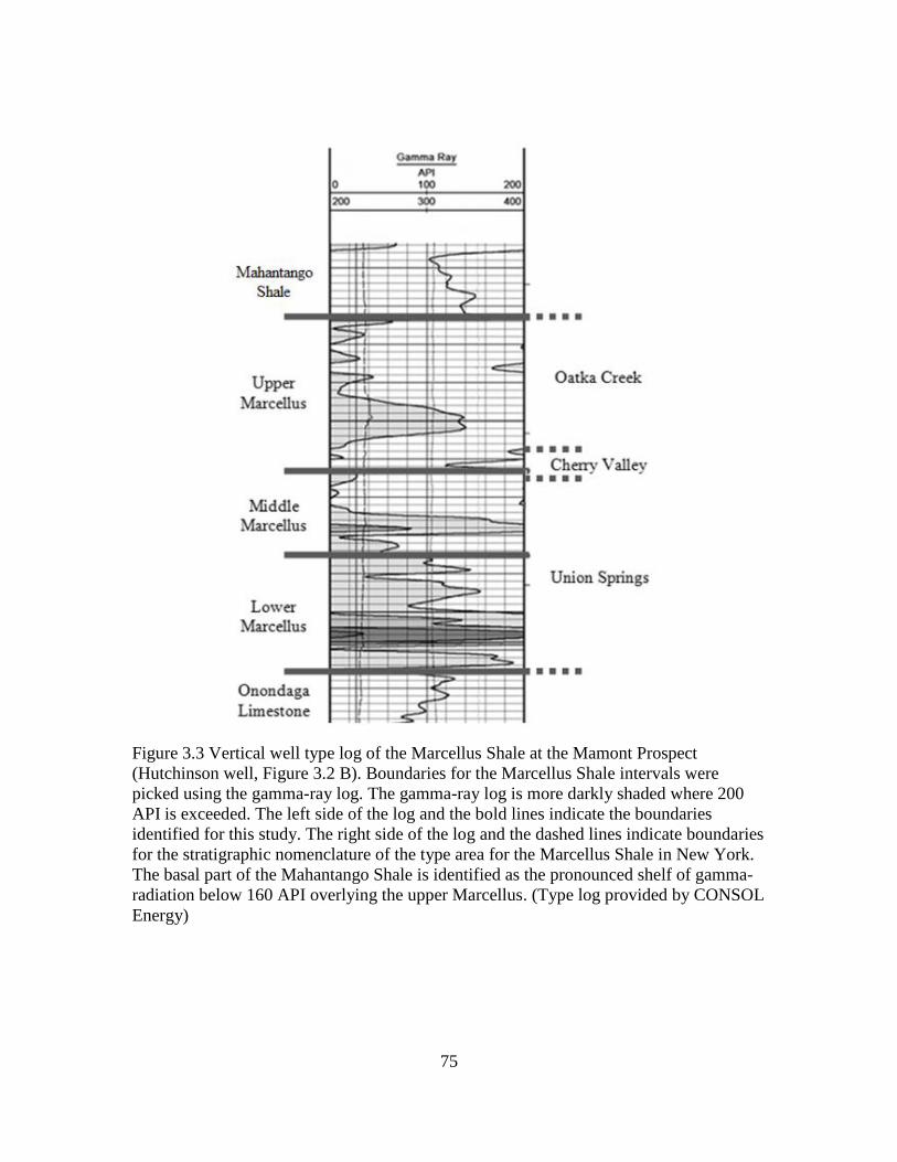
75

Figure 3.3 Vertical well type log of the Marcellus Shale at the Mamont Prospect

(Hutchinson well, Figure 3.2 B). Boundaries for the Marcellus Shale intervals were

picked using the gamma-ray log. The gamma-ray log is more darkly shaded where 200

API is exceeded. The left side of the log and the bold lines indicate the boundaries

identified for this study. The right side of the log and the dashed lines indicate boundaries

for the stratigraphic nomenclature of the type area for the Marcellus Shale in New York.

The basal part of the Mahantango Shale is identified as the pronounced shelf of gamma-

radiation below 160 API overlying the upper Marcellus. (Type log provided by CONSOL

Energy)

76

Figure 3.4 Complex depth shift performed on the Mountain vertical well and Hutchinson

4G horizontal well. LWD and wire-line gamma-ray logs were stratigraphically aligned

by adding tie lines to correlative points from each log.

77

Figure 3.5 TG calibrated on the basal part of the Mahantango Shale to 350 gas units.

Calibration was used to help disclaim inaccurate gas response from mud-logging

instrumentation (i.e., gas traps). TG mean represents a mean TG value determined for

each well’s LL. TGTRAP mean represents a mean TG value after a zero adjustment was

performed. See Table 3.2 for well names and corresponding well numbers.

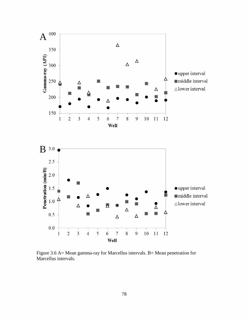
78

Figure 3.6 A= Mean gamma-ray for Marcellus intervals. B= Mean penetration for

Marcellus intervals.

A

B

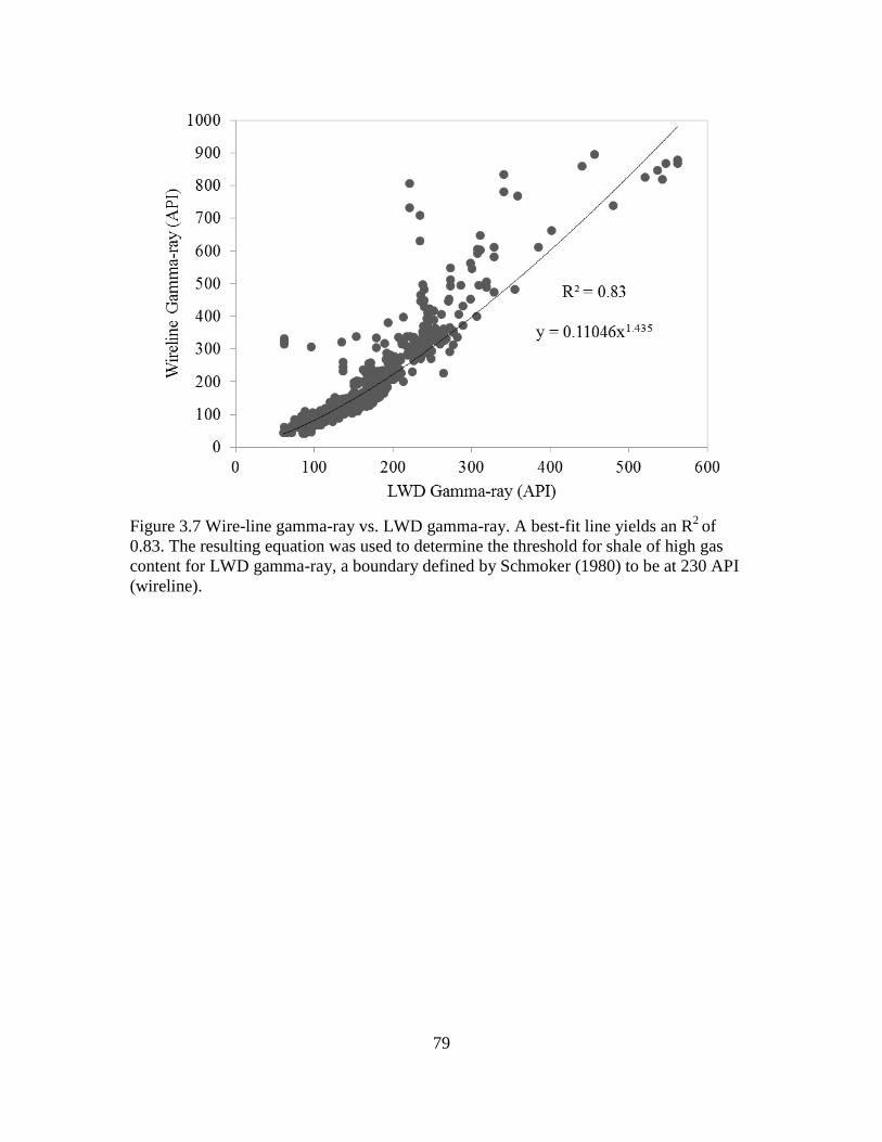
79

Figure 3.7 Wire-line gamma-ray vs. LWD gamma-ray. A best-fit line yields an R2

of

0.83. The resulting equation was used to determine the threshold for shale of high gas

content for LWD gamma-ray, a boundary defined by Schmoker (1980) to be at 230 API

(wireline).

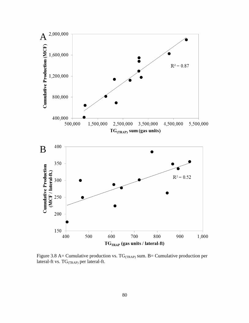
80

Figure 3.8 A= Cumulative production vs. TG(TRAP) sum. B= Cumulative production per

lateral-ft vs. TG(TRAP) per lateral-ft.

A

B

81

B

Figure 3.9 A= Cumulative production vs. TG(PH) sum. B= Cumulative production per

lateral-ft vs. TG(PH) per lateral-ft.

R2=0.40

A

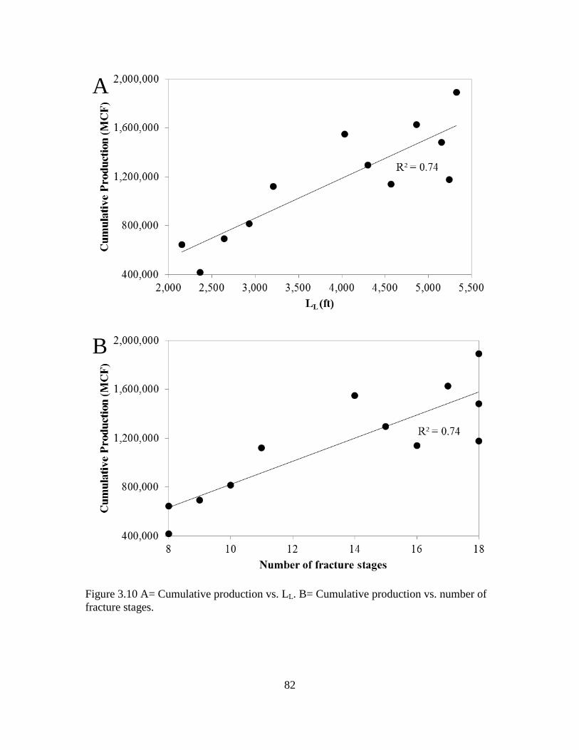
82

Figure 3.10 A= Cumulative production vs. LL. B= Cumulative production vs. number of

fracture stages.

A

B

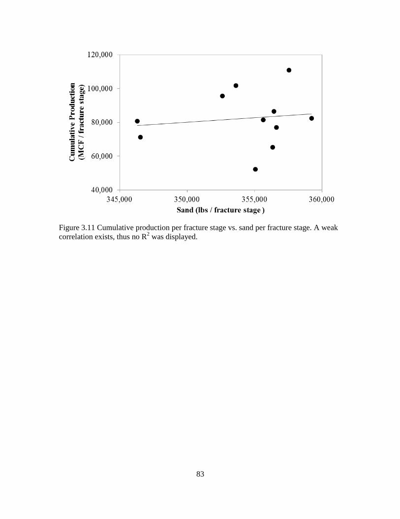
83

Figure 3.11 Cumulative production per fracture stage vs. sand per fracture stage. A weak

correlation exists, thus no R2 was displayed.

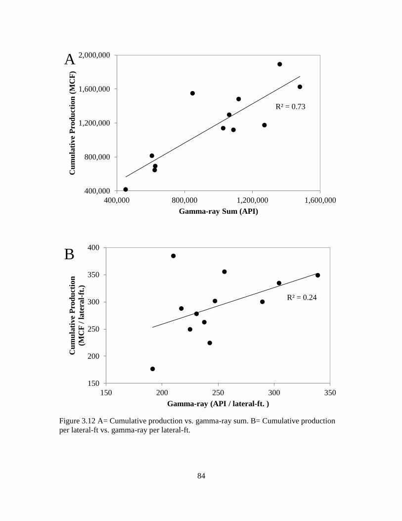
84

Figure 3.12 A= Cumulative production vs. gamma-ray sum. B= Cumulative production

per lateral-ft vs. gamma-ray per lateral-ft.

R² = 0.24

150

200

250

300

350

400

150 200 250 300 350

Cu

mu

lati

ve

Pro

du

ctio

n

(MC

F /

late

ral-

ft.)

Gamma-ray (API / lateral-ft. )

R² = 0.73

400,000

800,000

1,200,000

1,600,000

2,000,000

400,000 800,000 1,200,000 1,600,000

Cu

mu

lati

ve

Pro

du

ctio

n (

MC

F)

Gamma-ray Sum (API)

B

A

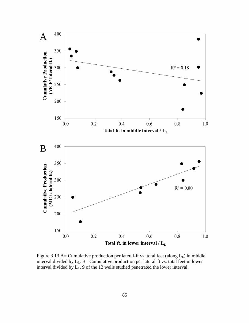
85

Figure 3.13 A= Cumulative production per lateral-ft vs. total feet (along LL) in middle

interval divided by LL. B= Cumulative production per lateral-ft vs. total feet in lower

interval divided by LL. 9 of the 12 wells studied penetrated the lower interval.

B

A

86

CHAPTER FOUR: CONCLUSIONS

For the Marcellus Shale of the Mamont Prospect, pseudo-density values were

estimated from gamma-ray logs to replace potentially inaccurate bulk-density values in

rugose sections of borehole in vertical wells. Increased organic matter content in

stratigraphically descending Marcellus Shale intervals was interpreted from calculated

mean values of gamma-ray, bulk-density, and resistivity. The modified Archie formula

yielded a 0.016 mean SW in the lower Marcellus and 0.166 mean SW in the upper

Marcellus, compared to 0.121 and 0.314, respectively, calculated from the standard

Archie formula. Formulas from Core Laboratories, derived from the bulk-density log,

yielded 0.114 mean PHI and 6.9% mean TOC in the lower Marcellus interval. The

structural deepening of the underlying Onondaga Limestone follows trend of increased

natural gas potential in the Mamont Prospect. Increased natural gas potential corresponds

to net productive Marcellus Shale thickness (i.e., gamma-ray >230 API and bulk density

< 2.55 g/cc).

Increased organic matter content and possibly greater over pressure in

stratigraphically descending Marcellus Shale intervals was interpreted from calculated

mean values of gamma-ray and penetration along the LL of horizontal wells. The upper

Marcellus interval (187 API mean) falls beneath the threshold for shale of high gas

content, which was determined to be at 205 API for LWD gamma-ray. Calibrated TG

measurements (TGTRAP and TGPH) show correspondence with cumulative production

(R2=0.87 and R

2=0.70, respectively). TGTRAP and TGPH measurements (on a per lateral-ft.

basis) showed correspondence with cumulative production per lateral-ft (R2=0.52 and

R2=0.40, respectively). For every 1000 feet of LL, production increases approximately

87

215,000 MCF. The correlation between percent of LL in the lower Marcellus interval and

cumulative production per lateral-ft (R2=0.80) indicates that the lower Marcellus

contributes largely to production.

88

Tab

le 4

.1 C

hap

ter

2 s

um

mary

of

resu

lts.

Dis

trib

uti

on

Par

amet

er

Fin

din

gs

Evid

ence

/Support

Ver

tica

l

Tota

l o

rgan

ic c

arb

on

(T

OC

)

Incr

ease

s in

str

atig

raphic

ally

des

cendin

g

aMar

cell

us

inte

rval

s

Mea

n g

amm

a-r

ay,

bu

lk-d

ensi

ty,

and

a

re

sist

ivit

y i

ncr

ease

in

str

atig

rap

hic

ally

a

d

esce

nd

ing

Mar

cell

us

inte

rval

s

Bu

lk-d

ensi

ties

inte

gra

ted

into

form

ula

s fr

om

a

C

ore

Lab

ora

tori

es

PH

I In

crea

ses

in s

trat

igra

phic

ally

des

cendin

g

aMar

cell

us

inte

rval

s

Bu

lk-d

ensi

ties

inte

gra

ted

into

form

ula

s fr

om

a

C

ore

Lab

ora

tori

es

*S

W (

mo

d) an

d S

W (

std)

Incr

ease

s in

str

atig

raphic

ally

des

cendin

g

aMar

cell

us

inte

rval

s

Inte

gra

tio

n o

f co

mp

on

ents

(T

h a

nd

U)

of

the

a

sp

ectr

al g

amm

a-r

ay l

og i

nto

the

mo

dif

ied

a

A

rch

ie F

orm

ula

Lat

eral

_(m

aps)

Gam

ma-r

ay >

23

0 A

PI

M

arce

llus

thic

knes

s in

crea

ses

from

anort

hea

st M

amont

tow

ards

the

wes

t

Lat

eral

tre

nds

ob

serv

ed i

n i

sop

ach m

ap

*G

amm

a-r

ay >

23

0 A

PI

and

__

Bu

lk-d

ensi

ty <

2.5

5 g

/cc

__

Mar

cell

us

thic

knes

s in

crea

ses

from

anort

hea

st M

amont

tow

ards

the

south

wes

t

Foll

ow

s st

ruct

ura

l dee

pen

ing o

f O

nondag

a

aLim

esto

ne

Lat

eral

tre

nds

ob

serv

ed i

n i

sop

ach m

ap

Ura

niu

m >

30

pp

m

Mar

cell

us

thic

knes

s in

crea

ses

from

south

aMam

ont

tow

ards

the

wes

t

Lat

eral

tre

nds

ob

serv

ed i

n i

sop

ach m

ap

*S

W (

mo

d) an

d S

W (

std)

Incr

ease

s fr

om

the

Bow

man

wel

l in

the

asouth

tow

ards

the

Ger

mro

th w

ell

in t

he

awes

t an

d t

he

Pola

har

wel

l in

the

east

Lat

eral

tre

nds

ob

serv

ed i

n i

so-S

W m

aps

*P

HI

G

reat

er i

n t

he

vic

init

y o

f th

e A

iken

s w

ell

athan

in o

ther

are

as o

f th

e M

amont

aPro

spec

t

Lat

eral

tre

nds

ob

serv

ed i

n i

so-p

oro

sity

map

*T

OC

> 7

%

Gre

ater

in t

he

vic

init

y o

f th

e A

iken

s w

ell

ath

an i

n o

ther

are

as o

f th

e M

amo

nt

Pro

spec

t

Lat

eral

tre

nds

ob

serv

ed i

n i

sop

ach m

ap

* C

alcu

late

d f

or

net

pro

du

ctiv

e M

arce

llus

Shal

e

89

APPENDICES

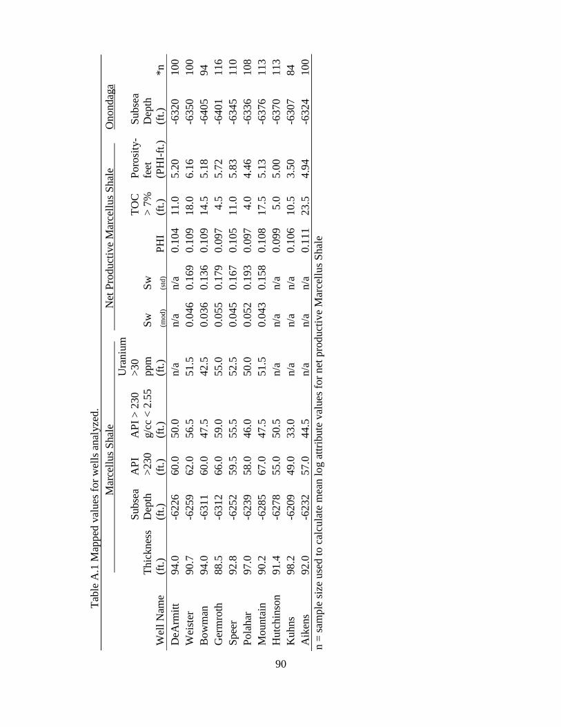
90

T

able

A.1

Map

ped

val

ues

for

wel

ls a

nal

yze

d.

M

arce

llus

Shal

e

N

et P

roduct

ive

Mar

cell

us

Shal

e

O

nondag

a

Wel

l N

ame

Thic

knes

s

(ft.

)

Subse

a

Dep

th

(ft.

)

AP

I

>230

(ft.

)

AP

I >

230

g/c

c <

2.5

5

(ft.

)

Ura

niu

m

>30

ppm

(ft.

)

Sw

(mod

)

Sw

(std

)

PH

I

TO

C

> 7

%

(ft.

)

Poro

sity

-

feet

(PH

I-ft

.)

Sub

sea

Dep

th

(ft.

) *n

D

eArm

itt

94.0

-6

226

60.0

50.0

n/a

n/a

n/a

0.1

04

11.0

5.2

0

-63

20

100

W

eist

er

90.7

-6

259

62.0

56.5

51.5

0.0

46

0.1

69

0.1

09

18.0

6.1

6

-63

50

100

B

ow

man

94.0

-6

311

60.0

47.5

42.5

0.0

36

0.1

36

0.1

09

14.5

5.1

8

-64

05

94

G

erm

roth

88.5

-6

312

66.0

59.0

55.0

0.0

55

0.1

79

0.0

97

4.5

5.7

2

-64

01

116

S

pee

r 92.8

-6

252

59.5

55.5

52.5

0.0

45

0.1

67

0.1

05

11.0

5.8

3

-63

45

110

P

ola

har

97.0

-6

239

58.0

46.0

50.0

0.0

52

0.1

93

0.0

97

4.0

4.4

6

-63

36

108

M

ounta

in

90.2

-6

285

67.0

47.5

51.5

0.0

43

0.1

58

0.1

08

17.5

5.1

3

-63

76

113

H

utc

hin

son

91.4

-6

278

55.0

50.5

n/a

n/a

n/a

0.0

99

5.0

5.0

0

-63

70

113

K

uh

ns

98.2

-6

209

49.0

33.0

n/a

n/a

n/a

0.1

06

10.5

3.5

0

-63

07

84

A

iken

s 92.0

-6

232

57.0

44.5

n/a

n/a

n/a

0.1

11

23.5

4.9

4

-63

24

100

n =

sam

ple

siz

e use

d t

o c

alcu

late

mea

n l

og a

ttri

bute

val

ues

for

net

pro

duct

ive

Mar

cell

us

Shal

e

91

Tab

le A

.2 C

alcu

late

d v

alues

use

d i

n h

ori

zonta

l w

ell

cross

-plo

ts.

.

Val

ues

sum

med

alo

ng L

L V

alu

es p

er l

ater

al-f

t. .

T

ota

l fe

et /

LL

Wel

l #

Wel

l N

ame

1T

GT

RA

P

2T

GP

H

3T

GT

RA

P

4T

GP

H

5G

R

mid

dle

lo

wer

1

DeA

rmit

t 1A

1,8

86

,372

7,3

62,1

36

644

1825

220

0.3

5

0.5

4

2

DeA

rmit

t 1C

3,1

33

,756

15,7

76,6

65

777

2226

206

0.9

5

n/a

3

Hutc

hin

son 4

A

2,2

25

,911

5,7

93,5

94

843

1725

219

0.3

9

0.5

3

4

Hutc

hin

son 4

B

9

58

,410

1,8

45,3

97

405

1197

196

0.8

4

0.1

0

5

Hutc

hin

son 4

C

3,1

00

,311

1

73,2

47

721

1881

226

0.9

5

n/a

6

Hutc

hin

son 4

D

2,1

60

,713

4,8

81,7

19

473

1004

246

0.8

5

0.0

5

7

Hutc

hin

son 4

E

2,7

85

,062

4,6

67,9

41

868

1468

329

0.0

7

0.8

3

8

Hutc

hin

son 4

F

9

97

,499

2,4

57,5

30

463

1234

273

0.0

8

0.8

4

9

Hutc

hin

son 4

G

4,3

35

,070

6,4

41,6

10

892

1227

305

0.0

4

0.9

2

10

Hutc

hin

son 4

H

3,2

24

,040

4,7

84,1

65

615

876

230

0.9

7

n/a

11

Hutc

hin

son 4

I 3

,139,5

67

6,2

73,7

28

610

1175

224

0.3

2

0.6

5

12

Hutc

hin

son 4

J 5

,015

,386

11,2

97,5

40

942

1996

240

0.0

3

0.9

5

1 [

gas

unit

s]

2 [

gas

unit

s-m

in/f

t3]

3 [

gas

unit

s /

late

ral-

ft]

4 [

gas

unit

s-m

in/f

t3 /

late

ral-

ft]

5 [

AP

I]

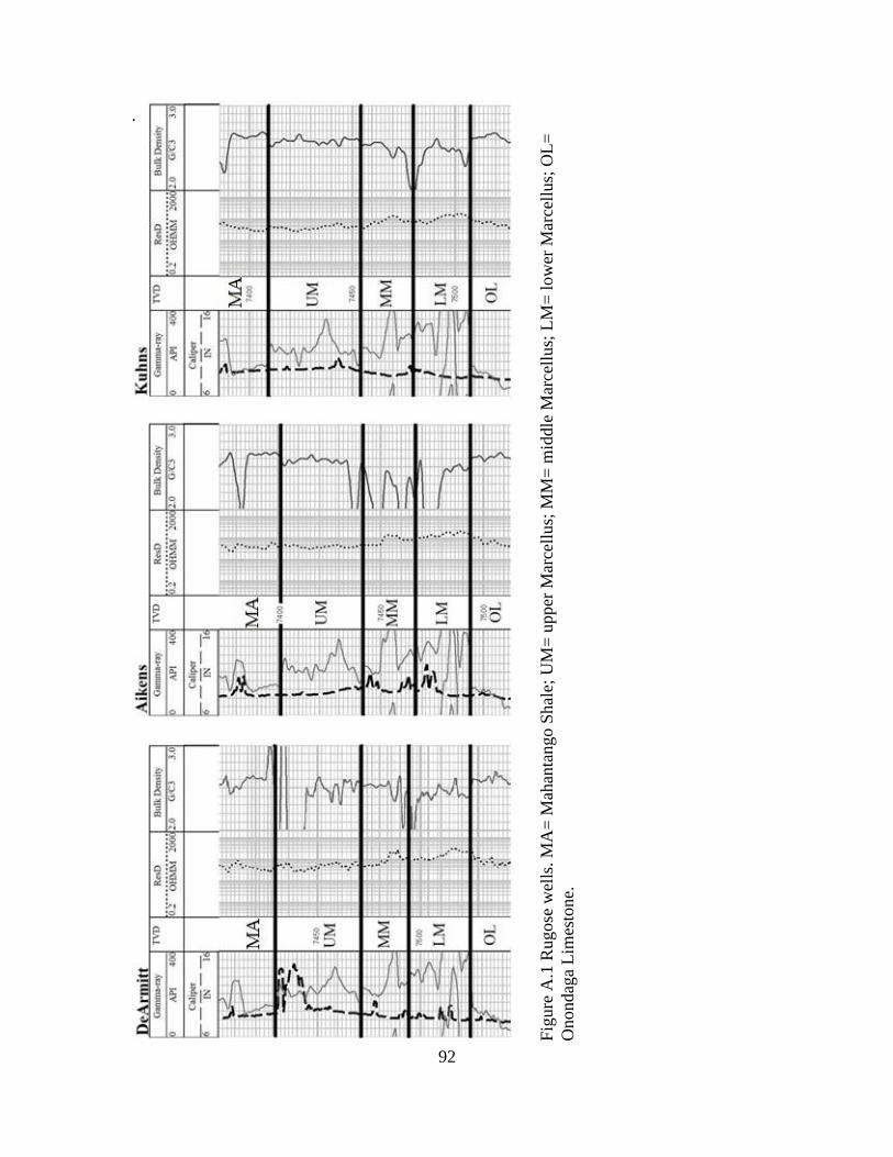
92

.

Fig

ure

A.1

Rugose

wel

ls. M

A=

Mah

anta

ngo S

hal

e; U

M=

upper

Mar

cell

us;

MM

= m

iddle

Mar

cell

us;

LM

= l

ow

er M

arce

llus;

OL

=

Onondag

a L

imes

tone.

93

Fig

ure

A.2

Wel

l-lo

gs

of

the

Ger

mro

th a

nd M

ounta

in w

ells

show

ing M

arce

llus

Shal

e in

terv

als.

94

Fig

ure

A.3

Wel

l-lo

gs

of

the

Pola

har

and W

eist

er w

ells

show

ing M

arce

llus

Shal

e in

terv

als.

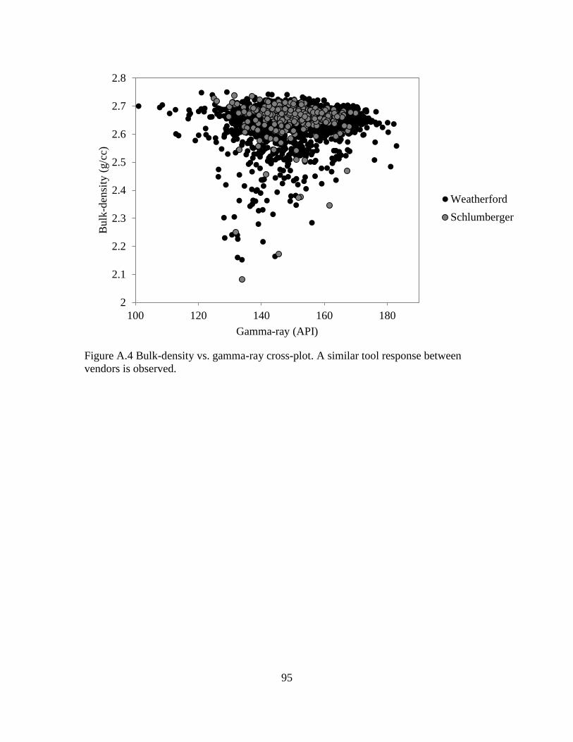
95

Figure A.4 Bulk-density vs. gamma-ray cross-plot. A similar tool response between

vendors is observed.

2

2.1

2.2

2.3

2.4

2.5

2.6

2.7

2.8

100 120 140 160 180

Bulk

-den

sity

(g/c

c)

Gamma-ray (API)

Weatherford

Schlumberger

96

Figure A.5 Parameters affecting cross-plot of bulk-density vs. gamma-ray in Devonian

Shales (modified from Fertl and Chilingar, 1988).

97

Fig

ure

A.6

DeA

rmit

t 1A

sin

gle

wel

l dia

gra

m s

ho

win

g g

amm

a-ra

y l

og, fr

actu

re s

tages

, an

d M

arce

llus

Shal

e in

terv

al p

osi

tion

of

wel

lbore

. U

M=

upper

Mar

cell

us;

MM

= m

iddle

Mar

cell

us;

LM

= l

ow

er M

arce

llus.

Fig

ure

A.7

DeA

rmit

t 1C

sin

gle

wel

l dia

gra

m s

ho

win

g g

amm

a-ra

y l

og, fr

actu

re s

tages

, an

d M

arce

llus

Shal

e in

terv

al p

osi

tion

of

wel

lbore

. U

M=

upper

Mar

cell

us;

MM

= m

iddle

Mar

cell

us;

LM

= l

ow

er M

arce

llus.

98

Fig

ure

A.8

Hutc

hin

son 4

A s

ingle

wel

l dia

gra

m s

how

ing g

amm

a-ra

y l

og, fr

actu

re s

tag

es, an

d M

arce

llus

Shal

e in

terv

al

posi

tion o

f w

ellb

ore

. U

M=

upper

Mar

cell

us;

MM

= m

iddle

Mar

cell

us;

LM

= l

ow

er M

arce

llus.

Fig

ure

A.9

Hutc

hin

son 4

B s

ingle

wel

l dia

gra

m s

ho

win

g g

amm

a-ra

y l

og, fr

actu

re s

tag

es, an

d M

arce

llus

Shal

e in

terv

al

posi

tion o

f w

ellb

ore

. U

M=

upper

Mar

cell

us;

MM

= m

iddle

Mar

cell

us;

LM

= l

ow

er M

arce

llus.

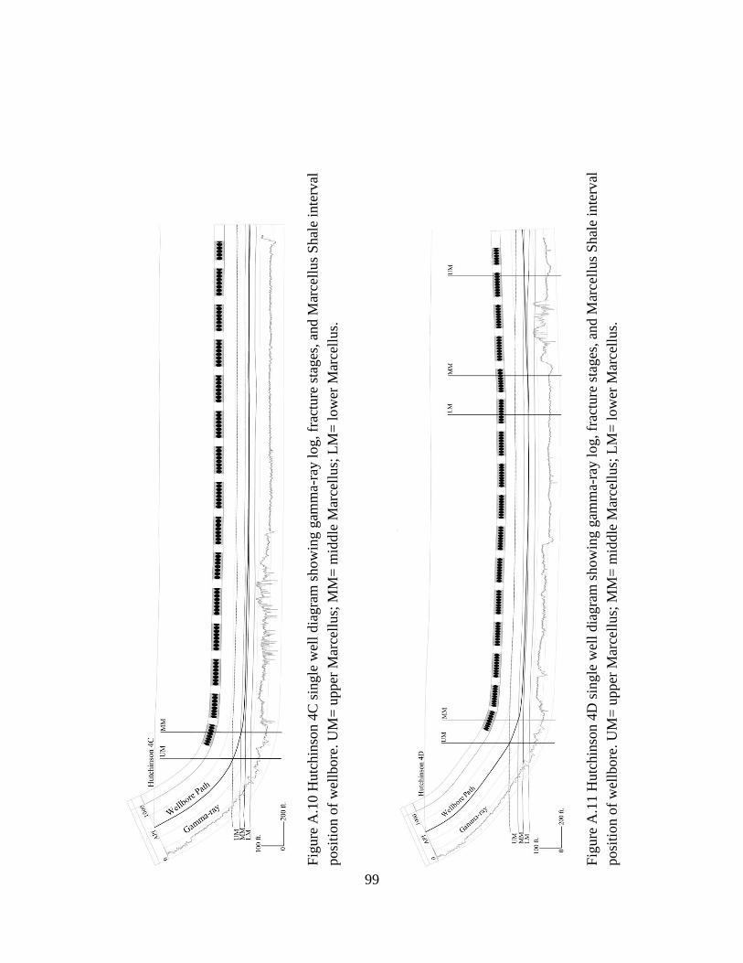
99

Fig

ure

A.1

0 H

utc

hin

son 4

C s

ingle

wel

l dia

gra

m s

ho

win

g g

amm

a-ra

y l

og, fr

actu

re s

tages

, an

d M

arce

llus

Shal

e in

terv

al

posi

tion o

f w

ellb

ore

. U

M=

upper

Mar

cell

us;

MM

= m

iddle

Mar

cell

us;

LM

= l

ow

er M

arce

llus.

Fig

ure

A.1

1 H

utc

hin

son 4

D s

ingle

wel

l dia

gra

m s

how

ing g

amm

a-ra

y l

og, fr

actu

re s

tages

, an

d M

arce

llus

Shal

e in

terv

al

posi

tion o

f w

ellb

ore

. U

M=

upper

Mar

cell

us;

MM

= m

iddle

Mar

cell

us;

LM

= l

ow

er M

arce

llus.

100

Fig

ure

A.1

2 H

utc

hin

son 4

E s

ingle

wel

l dia

gra

m s

how

ing g

amm

a-ra

y l

og, fr

actu

re s

tages

, an

d M

arce

llus

Shal

e in

terv

al

posi

tion o

f w

ellb

ore

. U

M=

upper

Mar

cell

us;

MM

= m

iddle

Mar

cell

us;

LM

= l

ow

er M

arce

llus.

Fig

ure

A.1

3 H

utc

hin

son 4

F s

ingle

wel

l dia

gra

m s

ho

win

g g

amm

a-ra

y l

og, fr

actu

re s

tages

, an

d M

arce

llus

Shal

e in

terv

al

posi

tion o

f w

ellb

ore

. U

M=

upper

Mar

cell

us;

MM

= m

iddle

Mar

cell

us;

LM

= l

ow

er M

arce

llus.

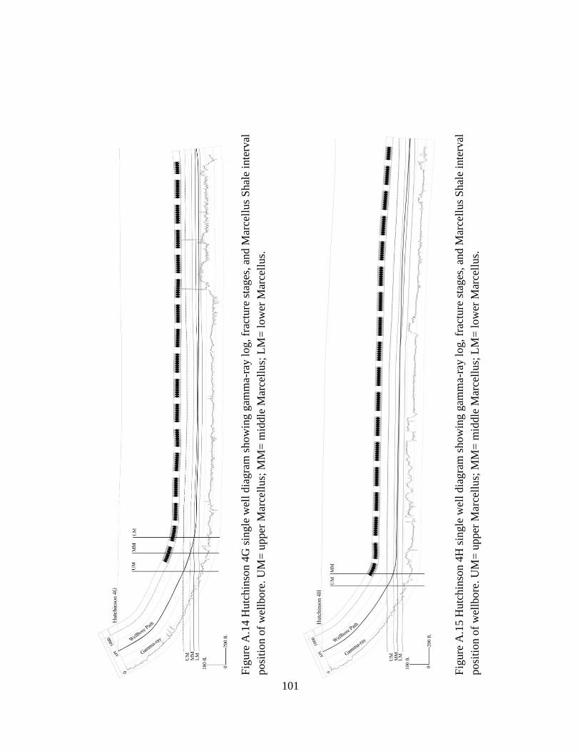
101

Fig

ure

A.1

4 H

utc

hin

son 4

G s

ingle

wel

l dia

gra

m s

how

ing g

amm

a-ra

y l

og, fr

actu

re s

tages

, an

d M

arce

llus

Shal

e in

terv

al

posi

tion o

f w

ellb

ore

. U

M=

upper

Mar

cell

us;

MM

= m

iddle

Mar

cell

us;

LM

= l

ow

er M

arce

llus.

Fig

ure

A.1

5 H

utc

hin

son 4

H s

ingle

wel

l dia

gra

m s

how

ing g

amm

a-ra

y l

og, fr

actu

re s

tages

, an

d M

arce

llus

Shal

e in

terv

al

posi

tion o

f w

ellb

ore

. U

M=

upper

Mar

cell

us;

MM

= m

iddle

Mar

cell

us;

LM

= l

ow

er M

arce

llus.

102

Fig

ure

A.1

6 H

utc

hin

son 4

I si

ngle

wel

l dia

gra

m s

how

ing g

amm

a-ra

y l

og, fr

actu

re s

tag

es, an

d M

arce

llus

Shal

e in

terv

al

posi

tion o

f w

ellb

ore

. U

M=

upper

Mar

cell

us;

MM

= m

iddle

Mar

cell

us;

LM

= l

ow

er M

arce

llus.

Fig

ure

A.1

7 H

utc

hin

son 4

J si

ngle

wel

l dia

gra

m s

how

ing g

amm

a-ra

y l

og, fr

actu

re s

tag

es, an

d M

arce

llus

Shal

e in

terv

al

posi

tion o

f w

ellb

ore

. U

M=

upper

Mar

cell

us;

MM

= m

iddle

Mar

cell

us;

LM

= l

ow

er M

arce

llus.

103

Figure A.18 Cumulative production vs. EUR. Correspondence between forcasted ultimate

production (EUR) and 18 months cumulative production is observed. Since EUR is a

forecast and has the potential to have error, 18 months cumulative production was used

in this investigation.

References

Fertl, W. & Chilingar, G. (1988). Total organic carbon content determined from well

logs. SPE Formation Evaluation, 3(2), 407-419.