Robotics: Science and Systems 2014Berkeley, CA, USA, July 12-16, 2014

1

Scene Signatures: Localised and Point-lessFeatures for LocalisationColin McManus1, Ben Upcroft2, and Paul Newman1

Abstract—This paper is about localising across extreme light-ing and weather conditions. We depart from the traditionalpoint-feature-based approach since matching under dramaticappearance changes is a brittle and hard. Point-feature detectorsare rigid procedures which pass over an image examining small,low-level structure such as corners or blobs. They apply thesame criteria to all images of all places. This paper takes acontrary view and asks what is possible if instead we learn abespoke detector for every place. Our localisation task then turnsinto curating a large bank of spatially indexed detectors andwe show that this yields vastly superior performance in termsof robustness in exchange for a reduced but tolerable metricprecision. We present an unsupervised system that producesbroad-region detectors for distinctive visual elements, called scenesignatures, which can be associated across almost all appearancechanges. We show, using 21 km of data collected over a periodof 3 months, that our system is capable of producing metricestimates from night-to-day or summer-to-winter conditions.

I. INTRODUCTION

Matching point features between different images is thestandard approach in visual motion estimation and has led to anumber of impressive systems for pose estimation and/or map-ping over large scales (e.g., Visual Teach & Repeat (VT&R)[1], and Visual Simultaneous Localisation And Mapping (VS-LAM) [2]). Matching low-level features such as edges, blobs,or corners works well when observing the same scene undersimilar conditions (e.g., for online ego-motion estimation).However, when trying to match images taken at different timesof day or in different seasons, these low-level features oftenlook utterly different. Larger image structures on the otherhand, such as windows, signs, or doors, offer more hope asthey capture shape and texture on a broader scale. We willshow that if we are careful about how we identify suitablestructures – which we shall refer to as scene signatures –then they can be reliably matched under large variations inappearance, thus opening the door to robust localisation.

Low-level point features can be thought of as being onone extreme of a localisation paradigm, while using whole-image information, such as SeqSLAM [3], can be thought ofas being on the opposite end of that spectrum. However, itshould be noted that SeqSLAM just provides an estimate onthe topological location of the vehicle and not a metric poseestimate. If we wish to provide a vehicle controller with ametric pose estimate, we need something in between thesetwo approaches.

1Mobile Robotics Group, University of Oxford, Oxford, England;{colin,pnewman}@robots.ox.ac.uk

2Robotics and Aerospace Systems, Queensland University of Technology,Brisbane, Australia; ben.upcroft@qut.edu.au

Visual MemoryLive Stream

(a) By matching scene signatures from a live stream (left) to a memory (right),we are able to successfully localise our vehicle.

(b) By matching point features from a live stream (left) to a memory (right),we are unable to successfully localise our vehicle.

Fig. 1. An illustration of the benefits of matching scene signatures, which aredistinctive visual elements such as fences, windows, tree lines, etc., versus thetraditional point-feature approach. Using point features for data associationunder extreme appearance changes often fails because point features onlyconsider low-level structure, like edges, corners, or blobs. Scene signaturesare more robust since they are large, distinctive elements.

In this paper, we present an unsupervised approach to finddistinctive visual elements, such as windows, signs, doors, ortree silhouettes (see Figure 1), in a given place, πp, which is anode in a hybrid topological/metric map. These are distinctivesignatures specific to the scene, and so we refer to them asscene signatures. We wish to stress that the benefit of usingscene signatures over point features is that we can associatethese scene signatures across extreme appearance changes,such as night to day or sunny to winter.

We shall constrain ourselves to the task of teaching avehicle, for example an autonomous car, to localise usingvision. We assume that the vehicle has or will be driventhrough the environment on multiple occasions and so wehave many examples of the appearance of the places thevehicle drives through. Rather than building a map of pointfeatures against which to match point features detected atrun time, we will construct, in an unsupervised way, a large

set of spatially indexed classifiers, which are associated withtopological locations in the world. Each of these classifiersis carefully constructed to fire on a particular and distinctiveaspect of the environment at that particular place, πp. As thevehicle progresses through its environment, we will retrievethe classifiers, {ci}p, relevant to its location, πp, and use themto identify known structure in the live image feed. These broadlevel features are used to create a “weak localiser” of sufficientaccuracy to provide coarse local, metric information about thevehicle’s pose.

Immediately we should ask, “for what tasks is such preci-sion adequate?” We envision a hierarchical system in which atthe top level we have very crude topological localiser whichoutputs the gross location of the vehicle. This output drivesthe localiser described in this work which takes a topologicalhint and returns a metric position accurate in orientation butwith perhaps tens of centimeters in translational error. Weassert that for autonomous road-vehicle navigation and control,we only need a coarse metric estimate of the vehicle’s pose,after which, lower level lane following and/or curb detectionalgorithms can be applied to refine the estimate for a vehiclecontroller. This is a shift from the traditional methods thattry and obtain centimeter-level accuracy. For a road vehiclewith on-board obstacle avoidance and lane following software,global localisation accuracy to the half metre is sufficient.

The novel contributions of this paper are the following:(i) the introduction of “weak localisers,” which use scenesignatures to perform metric estimation, (ii) an unsupervisedmethod which finds distinctive scene signatures, and (iii) thevalidation on challenging datasets displaying extreme appear-ance changes, from full light to deep darkness.

II. BACKGROUND

Decades of work have been focused on designing interest-point detectors and descriptors that can identify repeatablefeatures and describe them using unique, compact representa-tions. The output of these systems has enabled efficient featurecorrespondence across images taken at different viewpoints.Popular corner detectors include Harris Corners [4] and FAST[5], while blob detection can be performed with the Laplacianof Gaussian or MSER [6]. A range of image-point descriptorsalso exist, for example SIFT [7], SURF [8], BRIEF [9], andORB [10] to name a few. However, all of these interest-pointdetectors/descriptors operate on small image patches, whichcan look entirely different under different lighting and/orweather conditions. We will show that scene signatures enablematching across extreme changes in appearance because theycontain large, distinctive elements in the image. Note that ourapproach is very different from the localisation and mappingsystems of Davison et al. [11], [12], which use image patchesas their landmarks. These methods still rely on interest-pointdetection to find the patches and they use small patches (e.g.,11× 11 pixels in size). By construction, scene signatures arelarge distinctive elements in the scene that can be matchedacross extreme appearance changes.

Recently, there has been a number of attempts to shiftaway from the traditional, straight forward approach of blindlyapplying an out-of-the-box point-feature detector/descriptorfor egomotion estimation and/or localisation. Richardson et al.[13] present a method for learning an optimal feature detectorfor Visual Odometry (VO) tasks. Their method searches thespace of convolution filters to find the detector that minimisesreprojection error. Although this method is aimed at improvingstandard detection methods for an application specific task, itstill focused on using point features, which works well for VO,but not for localisation (e.g., matching a sunny day against arainy day).

Lategahn et al. [14] present a method for learning an optimalwhole-image descriptor for place recognition. They use agenetic optimisation approach to find the optimal combina-tion of fundamental feature blocks to construct their optimaldescriptor. However, as with other methods, such as SeqSLAM[3], this can only inform the system of the topological positionof the vehicle; it does not provide a metric estimate, which isimportant for us as we are interested in controlling a vehicle.

Rublee et al. [10] developed a new feature called ORB,which builds upon the FAST [15] detector and the BRIEF[9] descriptor. They use a greedy learning algorithm forde-correlating BRIEF features under rotational invariance.However, as this is still based on low-level structure, dataassociation remains hard under extreme appearance change.Hundelshausen et al. [16] present a noteworthy descriptor thatgoes beyond point features and instead constructs a networkof nodes and directed edges, where each edge is a descriptorin the network, referred to as a “d-token”. However, becausethese descriptors directly sample pixel intensities, this wouldnot be suitable for the types of extreme appearance changeswe are considering.

Ultimately, we are concerned with the problem of long-term,robust localisation in outdoor environments, which experiencea great deal of appearance changes (e.g., time of day and/ortime of year). One approach to this problem would be asystem like experience-based navigation [17], which recordsdistinct visual experiences of the environment as the vehicletraverses. If the live video stream cannot be matched to a priorexperience, it means the appearance of the world has changedenough to warrant the creation of a new experience. Althoughthis is a feasible approach, we offer an alternative that triesto learn what elements in the environment are stable acrossall appearances. In this way, localisation is not done againstnumerous experiences, but rather just a collection of distinctivescene elements.

Recently, Doersch et al. [18] presented a method for extract-ing geo-distinctive image patches from a collection of imagesof London and Paris. Their method was able to find imagepatches, or visual elements, of windows, balconies, and streetsigns which clearly distinguished the Parisian streets from theLondon streets. The method is, in principle, very simple andrelies on a large amount of data and a cross-validation trainingscheme. This will be discussed further in the next section.We have applied this idea to the localisation problem to find

distinctive visual elements that are stable across a wide rangeof appearance changes, such as lighting differences and/orseasonal changes. We call these scene signatures. The benefitof using scene signatures instead of low-level point features,which look for corners, edges, or blobs, is that the dataassociation problem becomes less challenging, since scenesignatures are very distinctive (e.g., doors, signs, windows,etc). As we use a stereo camera as the primary sensor, wecan perform left-to-right matching and obtain 3D positioninformation for each scene signature. This allows us to swapout point features for scene signatures in a VO framework, inorder to produce metric pose estimates.

III. SYSTEM OVERVIEW

Here we describe the two main components of our system:(i) the notion of a “weak localiser” that uses scene signaturesfor pose estimation, and (ii) the offline training algorithmwhich produces the scene signatures. As we will show, usingscene signatures instead of point features offers vast improve-ments in robustness to extreme appearance changes, resultingin a more robust localisation system.

At a high level, the steps involved in our localisation systemwork as follows:

1) Initialisation in the map (e.g., place recognition system),2) Use dead reckoning (e.g., wheel odometry) to predict

what place, πp, the vehicle is close to and load the bankof SVM classifiers, {ci}p, associated with that place,

3) Provided that the vehicle is sufficiently close to thatplace (e.g., within several meters), we use each SVMclassifier at multiple scales to search for associations inthe live image,

4) For each association, we compute the 3D stereo land-marks and solve for the optimal transformation estimateagainst the map.

An illustration of our system is shown in Figure 2.

A. WEAK LOCALISERS

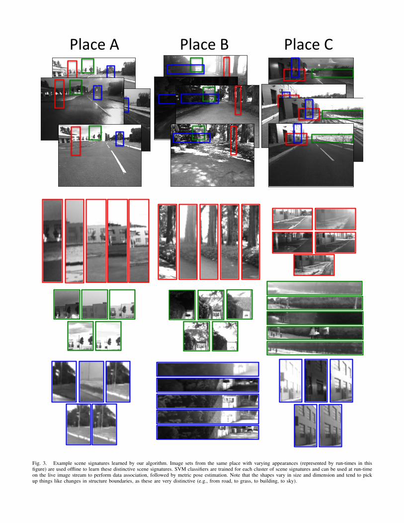
For a given place, πp, scene signatures represent distinctivevisual elements, such as buildings, trees, or distinctive struc-ture boundaries in the scene. Examples of scene signaturescan be seen in Figure 3. Note that each place is associatedwith a set of SVM classifiers trained on distinctive scenesignatures. We will show in the next section how these scenesignatures can be learned offline in an unsupervised manner.However, let us assume that for now we have access to abank of spatially indexed (for example by distance along aroad) SVM classifiers of scene signatures, {ci}p.

Although these scene signatures represent large areas in theimage, they can still provide a good metric idea of where thevehicle is locally. Additionally, because we can perform left-to-right matching between the stereo pair, each scene signaturehas an associated 3D point, allowing us to produce metricestimates local to each place.

In order to obtain sensible solutions, careful handling ofthe measurement uncertainties is required. The positionaluncertainty of a visual element in image space, Pzi , will be

SVM  classifiers  trained  on  patches  per  place  

Run  SVM  classifiers  in  regions  likely  to  

contain  the  patches  

Place  A  

Place  B  

Fig. 2. Offline, we learn scene signatures in the form of SVM classifiers.Each classifier is associated with a particular place, πp, and spatial regionin the image (i.e., the region that it’s most likely to fire in). At run-time,we use the bank of pretrained classifiers associated with πp to perform dataassociation and then localisation. By using larger, distinctive visual elements,we are able to localise in regions with extreme appearance change, where thepoint-feature-based counterpart fails.

a function of the scale, s, at which it was detected, the areaof the patch, a, the search resolution used when detecting thefeature, r, and the SVM detection probability, λ:

Pzi = f(a, r, s, λ). (1)

The relationship between the scale and search resolution isgiven by,

Pzi ∝1

sPr, (2)

where Pr is the noise covariance on the search resolution,which is scaled according to the pyramid level at which thedetector fires. The relationship with the other parameters,however, is less clear. Intuitively, we expect that the lowerthe probability of being a scene signature and the larger thearea of the patch, the less certain the keypoint position shouldbe. Thus, as a heuristic, we assume that the covariance takesthe following form,

Pzi :=a

λsPr. (3)

Although not considered here, another factor that may beuseful would be a level of confidence in the SVM score [19].

Since each patch feature, zj , has an associated 3D landmark,pj , we can use the standard stereo model, h(·), to predict thelocation of a landmark in frame b relative to some other framea, according to the transformation matrix, Ta,b:

zja = h(Ta,b,pjb) + nj

a, nja ∼ N (0,Pzj

a). (4)

Additionally, we use a strong prior, T̂a,b, with a smalluncertainty in the vertical offset between the live frame andthe map, as well as roll and pitch, since we know that thesepositional differences would be small for a road vehicle. Theprior is important because the translational component of the

Place  A   Place  B   Place  C  

Fig. 3. Example scene signatures learned by our algorithm. Image sets from the same place with varying appearances (represented by run-times in thisfigure) are used offline to learn these distinctive scene signatures. SVM classifiers are trained for each cluster of scene signatures and can be used at run-timeon the live image stream to perform data association, followed by metric pose estimation. Note that the shapes vary in size and dimension and tend to pickup things like changes in structure boundaries, as these are very distinctive (e.g., from road, to grass, to building, to sky).

localisation estimate will not be very accurate owing to the lownumber of patches in the foreground. However, we note thatwe obtain very good orientation estimates, so combined witha reasonable egomotion estimate from, say, wheel odometryor VO, the weak localisers are sufficient in providing poseestimates with similar accuracy as our INS system (i.e., submeters) in large outdoor environments. Including the priorestimate, T̂a,b, the final least-squares system we seek tooptimize is given by the following:

O(Ta,b) = (5)

1

2

[q(Ta,b, T̂a,b)

za − g(Ta,b,pb)

]T [P−1

x 00 P−1

z

] [q(Ta,b, T̂a,b)

za − g(Ta,b,pb)

],

where

za :=

z0a...

zMa

, pa :=

p0a...

zMp

, Pz := diag(Pz0a, . . . ,PzM

a),

(6)and q(·) is a function that takes two SE3 transformationmatrices and computes a 6×1 error vector, which depends onthe choice of the orientation parameterisation. Note that wealso use the Geman-McClure [20] robust cost function, whichleaves us with the following objective function:

O(Ta,b) =1

2

∑i

eTi P−1i ei

σ2i + eTi P

−1i ei

, (7)

where σi are the M-estimator parameters and each ei rep-resents an error term (e.g., the prior or measurement). Thishas the effect of scaling the covariance to down weight thecontribution of potential outliers during the iterative solve,which is done using Levenberg Marquardt [21].

B. UNSUPERVISED LEARNING OF SCENE SIGNATURES

This section will describe our unsupervised approach tolearning scene signatures, which are locally distinctive andstable visual elements. Locally distinctive means that the visualelement is distinct in a local region in image space. Given thatwe have a reasonable prior on the motion of the vehicle, it doesnot matter if the visual element occurs elsewhere in the image,it need only be locally distinctive for data association. Stablemeans that the visual element can be identified across multipleimages of the same area, under a variety of appearances.

The training algorithm can be divided into the followingsteps, where the main adaption of the algorithm described in[18] occurs in steps 1-3d.

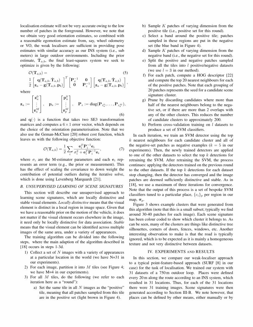
1) Collect a set of N images with a variety of appearancesat a particular location in the world (we have N=31 inour experiments).

2) For each image, partition it into M tiles (see Figure 4;we have M=4 in our experiments).

3) For all M tiles, do the following (we refer to eachiteration here as a “round”):

a) Set the same tile in all N images as the “positive”tile, meaning that all patches sampled from this tileare in the positive set (light brown in Figure 4).

b) Sample K patches of varying dimension from thepositive tile (i.e., positive set for this round).

c) Select a band around the positive tile; patchessampled in these regions are put in the negativeset (the blue band in Figure 4).

d) Sample K patches of varying dimension from thenegative band (i.e., the negative set for this round).

e) Split the positive and negative patches sampledfrom all the tiles into l positive/negative datasets(we use l = 3 in our method).

f) For each patch, compute a HOG descriptor [22]and compute the top 20 nearest neighbours for eachof the positive patches. Note that each grouping of20 patches represents the seed for a candidate scenesignature cluster.

g) Prune by discarding candidates where more thanhalf of the nearest neighbours belong to the nega-tive set, or if there are more than 2 overlaps withany of the other clusters. This reduces the numberof candidate clusters to approximately 200.

h) Perform cross-validation training on l datasets toproduce a set of SVM classifiers.

In each iteration, we train an SVM detector using the topk nearest neighbours for each candidate cluster and all ofthe negative-set patches as negative examples (k = 5 in ourexperiments). Then, the newly trained detectors are appliedto one of the other datasets to select the top k detections forretraining the SVM. After retraining the SVM, the processcontinues: applying the detectors trained on the previous roundto the other datasets. If the top k detections for each datasetstop changing, then the detector has converged and the imagepatches are deemed sufficiently distinctive and stable. As in[18], we use a maximum of three iterations for convergence.Note that the output of this process is a set of bespoke SVMclassifiers tuned to a particular place, {ci}p per region in ourmap, πp.

Figure 3 shows example clusters that were generated fromthis algorithm (note that this is a small subset; typically we findaround 30-40 patches for each image). Each scene signaturehas been colour coded to show which cluster it belongs to. Ascan be seen, many of the clusters are things like distinctive treesilhouettes, corners of doors, fences, windows, etc. Anotherinteresting observation to make is that the road is typicallyignored, which is to be expected as it is mainly a homogeneoustexture and not very distinctive between datasets.

IV. EXPERIMENTS AND RESULTS

In this section, we compare our weak-localiser approachto a typical point-feature-based approach (SURF [8] in ourcase) for the task of localisation. We trained our system with31 datasets of a 750 m outdoor loop. Places were definedevery 20 m along the route according to an INS system, whichresulted in 31 locations. Thus, for each of the 31 locationsthere were 31 training images. Scene signatures were thengenerated according to Section III-B. We note however, thatplaces can be defined by other means, either manually or by

Roun

d  1  

Roun

d  4  

31  images  per  place  

Fig. 4. Our strategy for partitioning the data to produce scene signatures. Wetake a collection of images at a particular location in the world and partitioneach image into a number of tiles. In this example, patches (black rectangles)drawn from the light brown regions are placed in the positive set and patchesdrawn from the blue regions are placed in the negative set. Since we have thesame pattern for every image and each image has roughly the same viewpoint,we are able to seed the training algorithm with elements subject to varyingappearance changes.

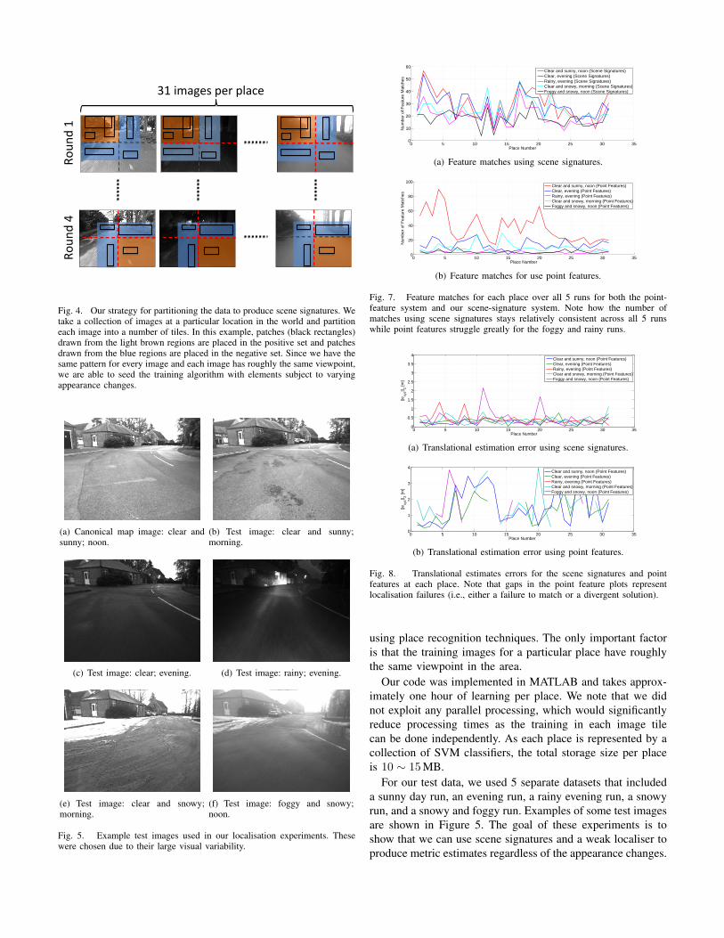
(a) Canonical map image: clear andsunny; noon.

(b) Test image: clear and sunny;morning.

(c) Test image: clear; evening. (d) Test image: rainy; evening.

(e) Test image: clear and snowy;morning.

(f) Test image: foggy and snowy;noon.

Fig. 5. Example test images used in our localisation experiments. Thesewere chosen due to their large visual variability.

0 5 10 15 20 25 30 350

10

20

30

40

50

60

Place Number

Num

ber

of F

eatu

re M

atch

es

Clear and sunny, noon (Scene Signatures)Clear, evening (Scene Signatures)Rainy, evening (Scene Signatures)Clear and snowy, morning (Scene Signatures)Foggy and snowy, noon (Scene Signatures)

(a) Feature matches using scene signatures.

0 5 10 15 20 25 30 350

20

40

60

80

100

Place Number

Num

ber

of F

eatu

re M

atch

es

Clear and sunny, noon (Point Features)Clear, evening (Point Features)Rainy, evening (Point Features)Clear and snowy, morning (Point Features)Foggy and snowy, noon (Point Features)

(b) Feature matches for use point features.

Fig. 7. Feature matches for each place over all 5 runs for both the point-feature system and our scene-signature system. Note how the number ofmatches using scene signatures stays relatively consistent across all 5 runswhile point features struggle greatly for the foggy and rainy runs.

0 5 10 15 20 25 30 350

0.5

1

1.5

2

2.5

3

3.5

4

Place Number

||exy

z|| 2 [m]

Clear and sunny, noon (Point Features)Clear, evening (Point Features)Rainy, evening (Point Features)Clear and snowy, morning (Point Features)Foggy and snowy, noon (Point Features)

(a) Translational estimation error using scene signatures.

0 5 10 15 20 25 30 350

1

2

3

4

Place Number

||exy

z|| 2 [m]

Clear and sunny, noon (Point Features)Clear, evening (Point Features)Rainy, evening (Point Features)Clear and snowy, morning (Point Features)Foggy and snowy, noon (Point Features)

(b) Translational estimation error using point features.

Fig. 8. Translational estimates errors for the scene signatures and pointfeatures at each place. Note that gaps in the point feature plots representlocalisation failures (i.e., either a failure to match or a divergent solution).

using place recognition techniques. The only important factoris that the training images for a particular place have roughlythe same viewpoint in the area.

Our code was implemented in MATLAB and takes approx-imately one hour of learning per place. We note that we didnot exploit any parallel processing, which would significantlyreduce processing times as the training in each image tilecan be done independently. As each place is represented by acollection of SVM classifiers, the total storage size per placeis 10 ∼ 15MB.

For our test data, we used 5 separate datasets that includeda sunny day run, an evening run, a rainy evening run, a snowyrun, and a snowy and foggy run. Examples of some test imagesare shown in Figure 5. The goal of these experiments is toshow that we can use scene signatures and a weak localiser toproduce metric estimates regardless of the appearance changes.

Live%Image% Map%Image%

(a) Clear, evening run.

Live%Image% Map%Image%

(b) Rainy, evening run.

Live%Image% Map%Image%

(c) Clear and snowy run.

Live%Image% Map%Image%

(d) Foggy and snowy run.

Fig. 6. Localisation results, where the arrows represent 2D projections of the vehicle coordinate frames for both methods. As both the point-feature and ourscene-signature method were able to localise all frames for the first dataset, we omitted the plots here and turn to the more challenging cases. Our scene-signature approach was able to localise all frames, whereas the point-feature-based system failed on 33% of the places. These failures have been indicated onthe plots with a large black circle. Note that almost all estimates agree to the INS ground truth within meters.

To reiterate, our localisation strategy is as follows. Afterinitialising in the map, we use dead reckoning to predict whenwe are within a couple meters of a place, after which we loadthe SVM classifiers associated with that place and run themon the live image to detect the scene signatures. Once wehave associated these scene signatures, we can perform local,metric, pose estimation. This approach of predicting wherethe nearest topological node is and then localising against themap is similar to teach-and-repeat systems such as McManuset al. [23] and Furgale and Barfoot [1], except that our mapkeyframes are separated by larger distances.

Figure 6 presents the localisation results for the 5 live runsagainst our map that contains a bank of trained classifiers perplace. The results show the live and reference INS trajectoriesas well as the localisation estimates for both our system andthe baseline. Unfortunately, as our INS system drifts onthe order of meters from one dataset to the next, it provedto be ill-suited to asses the accuracy of the estimates. Weinstead exploit the fact that the training images are gathered atapproximately the same position and use a generous toleranceon the translational/rotational estimates to define a localisation

TABLE INUMBER OF FRAMES LOCALISED AGAINST OUT OF 31 PLACES.

Live Run Scene Signatures Point FeaturesClear and sunny morning 31 31

Clear evening 31 28Rainy evening 31 9

Clear and snowy morning 31 24Foggy and snowy afternoon 31 12

failure. Letting x̂ := [t̂T , θ̂T ]T represent our estimate, wedefine a localisation failure if ||t̂||2 > α or ||θ̂||2 > β, wherewe chose α = 4m and β = 30◦.

Table I shows the number of frames localised against foreach run (according to INS ground truth), where we see thatour system was able to localise all frames in all 5 datasets,despite extreme variations in appearance. The point-feature-based system was unable to localise a majority of the framesfor the rainy evening run and the foggy snowy run. Figure 7shows the number of feature matches for each place over all5 runs. Figure 8 shows the estimation errors for each place.Figure 9 shows examples of our system succeeding where thepoint-feature system failed.

Fig. 9. Examples where our method was able to localise the live run (left image of each pair) with the map (right image of each pair), while point-featuresfailed. Only a subset of the matches are being shown for clarity. On average, we obtained 24 matches per place across all five datasets using scene signatures.

14/07/2014

Scene Signatures: Localised and Point-less Features for Localisation{colin, pnewman}@robots.ox.ac.uk, ben.upcroft@qut.edu.au

Run$me'Localisa$on

VO#Pose#

Localisa-on#

Ac-ve#Region#

•Detec%on(is(done(using(OpenCV’s(OpenCL(HOG•Runs(at(roughly(2=5Hz(in(a(separate(thread•Main(thread(uses(Visual(Odometry(to(predict(pose(in(between(localisa%ons((main(thread(runs(at(15=20(Hz)•Posegraph(relaxa%on(is(performed(over(a(local(sliding(window

Fig. 10. Illustration of our runtime localisation approach. Localisationupdates occur at 2-5 Hz, while Visual Odometry updates occur at 15-20 Hz.After we receive a localisation update, we perform posegraph relaxation overa sliding window, indicated by the active region in green.

V. SYSTEMS WORK

The results and method described in this paper representour initial iteration of the scene-signature approach, whichwas coded in Matlab and ran offline. We have since portedthe code to C++ to obtain realtime performance. Our linear-SVM detection class uses OpenCV’s OpenCL HOG for featureextraction. Our scene-signature detection block runs in aseparate thread at approximately 2-5 Hz. Our main thread runsVisual Odometry at approximately 15-20 Hz to predict posesin between localisations. As the localisation updates occur ata slower rate, we perform posegraph relaxation over a slidingwindow to obtain our final estimate (see Figure 10).

VI. DISCUSSION AND CONCLUSION

We have demonstrated a new approach to the localisationtask, which departs from the traditional point-feature systemby learning spatially indexed classifiers of distinctive visualelements called scene signatures. Although we are unable toobtain accuracy on the order of centimeters, we are morerobust to extreme appearance change and obtain the sametype of coverage as a topological localisation system, likeSeqSLAM [3], but with the added benefit of metric pose.

Scene signatures enable robust, metric localisation wheretraditional systems simply fail. Each bank of place-dependantSVM classifiers is run on the live image stream to performthe data association, and a standard frame-to-frame localisationframework is used to obtain the metric pose estimate. We haveshown that our approach can successfully localise the vehicleacross very challenging lighting and/or weather conditions. Webelieve that point features alone are simply not enough forrobust, long-term localisation systems and that our approachis a step in the right direction.

VII. ACKNOWLEDGEMENTS

This work would not have been possible without the fi-nancial support from the Nissan Motor Company, the EP-SRC Leadership Fellowship Grant (EP/J012017/1), and V-CHARGE (Grant Agreement Number 269916).

REFERENCES

[1] P. Furgale and T. Barfoot, “Visual teach and repeat for long-range roverautonomy,” Journal of Field Robotics, special issue on “Visual mappingand navigation outdoors”, vol. 27, no. 5, pp. 534–560, 2010.

[2] K. Konolige, J. Bowman, J. Chen, P. Mihelich, M. Calonder, V. Lepetit,and P. Fua, “View-based maps,” The International Journal of RoboticsResearch, vol. 29, no. 8, pp. 941–957, 2010.

[3] M. Milford and G. Wyeth, “Seqslam: Visual route-based navigation forsunny summer days and stormy winter nights,” in Proceedings of theIEEE International Conference on Robotics and Automation (ICRA),Saint Paul, Minnesota, USA, 14-18 May 2012.

[4] C. Harris and M. Stephens, “A combined corner and edge detector,” inProceedings of the 4th Alvey Vision Conference, 1988, pp. 147–151.

[5] E. Rosten, G. Reitmayr, and T. Drummond, “Real-time video annotationsfor augmented reality,” in Advances in Visual Computing, 2005.

[6] J. Matas, O. Chum, M. Urban, and T. Pajdla, “Robust Wide BaselineStereo from Maximally Stable Extremal Regions,” in Proceedings ofthe British Machine Vision Conference. BMVA Press, 2002, pp. 36.1–36.10, doi:10.5244/C.16.36.

[7] D. Lowe, “Distinctive image features from scale-invariant keypoints,”International Journal of Computer Vision, 2004.

[8] H. Bay, A. Ess, T. Tuytelaars, and L. Gool, “Surf: Speeded up robustfeatures,” Computer Vision and Image Understanding (CVIU), vol. 110,no. 3, pp. 346–359, 2008.

[9] M. Calonder, V. Lepetit, M. Ozuysal, T. Trzcinski, C. Strecha, andP. Fua, “Brief: Computing a local binary descriptor very fast,” IEEETransactions on Pattern Analysis and Machine Intelligence, vol. 34,no. 7, pp. 1281–1298, 2012.

[10] E. Rublee, V. Rabaud, K. Konolige, and G. Bradski, “Orb: An efficientalternative to sift or surf,” in IEEE International Conference on Com-puter Vision (ICCV), 2011, pp. 2564–2571.

[11] A. Davison, I. Reid, N. Motlon, and O. Stasse, “Monoslam: Real-time single camera slam,” IEEE Transactions on Pattern Analysis andMachine Intelligence, vol. 29, no. 6, 2007.

[12] A. Davison and D. Murray, “Simultaneous localization and map-building

using active vision,” IEEE Transactions on Pattern Analysis and Ma-chine Intelligence, vol. 24, no. 7, 2002.

[13] A. Richardson and E. Olson, “Learning convolutional filters for interestpoint detection,” in Proceedings of the IEEE International Conferenceon Robotics and Automation (ICRA), 2013.

[14] H. Lategahn, J. Beck, B. Kitt, and C. Stiller, “How to learn an illumi-nation robust image feature for place recognition,” in IEEE IntelligentVehicles Symposium, Gold Coast, Australia, 2013.

[15] E. Rosten and T. Drummond, “Machine learning for high-speed cornerdetection,” in European Conference on Computer Vision, 2006.

[16] F. von Hundelshausen and R. Sukthankar, “D-Nets: Beyond Patch-BasedImage Descriptors,” in IEEE International Conference on ComputerVision and Pattern Recognition, 2012.

[17] W. Churchill and P. Newman, “Practice makes perfect? managing andleveraging visual experiences for lifelong navigation,” in Proceedings ofthe International Conference on Robotics and Automation, Saint Paul,Minnesota, USA, 14-18 May 2012.

[18] C. Doersch, S. Singh, A. Gupta, J. Sivic, and A. Efros, “What makesparis look like paris?” ACM Transactions on Graphics, 2012.

[19] A. Pronobis and B. Caputo, “Confidence-based cue integration forvisual place recognition,” in Proceedings of the IEEE/RSJ InternationalConference on Intelligent Robotics and Systems, San Diego, California,USA, Oct 29 - Nov 2 2007.

[20] S. Geman and D. McClure, “Statistical method for tomographic imagereconstruction,” in Proceedings of the 46th Session of the InternationalStatistical Institute, Bulletin of the ISI, vol. 52, 1987, pp. 5–21.

[21] K. Levenberg, “A method for the solution of certain non-linear problemsin least squares,” The Quarterly of Applied Mathematics, vol. 2, pp. 164–168, 1944.

[22] N. Dalal and B. Triggs, “Histograms of oriented gradients for humandetection,” in Proceedings of the Conference on Computer Vision andPattern Recognition, San Diego, California, USA, 2005, pp. 886–893.

[23] C. McManus, P. Furgale, B. Stenning, and T. D. Barfoot, “Visual Teachand Repeat Using Appearance-Based Lidar,” in Proceedings of IEEEInternational Conference on Robotics and Automation (ICRA), 2012.