SOUTHERN JOURNAL OF AGRICULTURAL ECONOMICS JULY 1992

LIVESTOCK FUTURES MARKETS AND RATIONAL PRICEFORMATION: EVIDENCE FOR LIVE CATTLE AND LIVEHOGSStephen R. Koontz, Michael A. Hudson, and Matthew W. Hughes

Abstract Two roles of futures markets have been empha-.. he~~ '^cn o c . sized in analyses of market performance (Tomek and

The efficiency of livestock futures markets contin- Gray; Peck 1985 and 1987). The first role, the allo-ues to receive attention, particularly with regard to c r w i i b cative role, was investigated initially by Working intheir forward pricing or forecasting ability. The pur-theirforward cingorforecastingability.Thea study of grain basis relationships and storage costs.pose of this paper is to present a more general theory availability of futures contracts for storableThe availability of futures contracts for storablethat encompasses the forward pricing concept. It is commodities, deliverable upon out to a year in thecommodities, deliverable upon out to a year in theargued that futures contract prices for competitively f a future, are thought to provide price incentives whichproduced nonstorable commodities, such as live cat- influence storage decisions and thereby allocatetie and live hogs, follow arational formation process grain consumption through the crop year. AnalysisFutures contract prices reflect expected market con- of the secondrole,forwardpricing,emerged withtheditions when contracts are sufficiently close to the introduction offuturestradingsemi-storablecom-introduction of futures trading in semi-storable com-delivery month that the supply of the underlying modities(e.g.,onions potatoes)andnonstorablemodtfies (e.g., onions and potatoes) and nonstorablecommodity cannot be changed. However, prior to thecommoditycannotbechanged.However,priortothe commodities (e.g., livestock). It has been argued thatperiod when future supplies are relatively fixed,peod when future supplies are relatively fixed, price levels of futures contracts for nonstorable com-futures contract prices should adjust to reflect the moditiesdeliverableuponouttoyearinthefuture,modities, deliverable upon out to a year in the future,competitive equilibrium, where output price equals should forecast anticipated supply-emand coni-average costs ofproduction. Presented evidence sug- t i tions in these forward markets. Futures markets forgests that live cattle and live hog futures markets semi-storable commodities are thought to combinesupport the rational price formation hypothesis: tese toleprices for distant contracts reflect average costs of e A dilemma has emerged in the literature in thatfeeding. Implications for risk management strategiess r e it

futures markets for storable commodities performare considered. both the allocative and forward pricing roles well,while futures markets for nonstorable commodities

Key words: futures markets, rational price are typically poor forecasters (Leuthold and Hart-formation, forecasting performance, mann; Just and Rausser; Martin and Garcia; Shonk-forward pricing wiler). The conclusion often drawn is that the futures

T markets for nonstorable commodities are inefficient,In recent years, the efficiency of livestock futures that the speculators in these markets are not using allmarkets has received increased attention. Respond- available information, and that ex ante welfare lossesing to producer concerns that futures markets are are incurred by society (Stein).detrimental to the industry, researchers have exam- This paper examines the live cattle and live hogined the roles of livestock futures markets in discov- futures markets within the rational pricing frame-ering and forecasting prices, allocating resources to work suggested by Gray. At the outset, it is arguedproduction, and registering market information that early in its life a livestock futures contract trades(Purcell and Hudson). The results of these studies are in a price range around average costs of feeding.mixed and often depend on the time period and Early in the contract life is defined as the periodmethod of analysis (Garcia et al. 1988a). The avail- when the supply to be marketed during the deliveryable research suggests difficulties in drawing defini- month can be influenced by the futures prices. Oncetive conclusions about the efficiency of livestock the possibility of supply response is eliminatedfutures markets. through production commitments (e.g., when the

Stephen R. Koontz is Assistant Professor in the Department of Agricultural Economics at Oklahoma State University, Michael A.Hudson is an Associate Professor and Bruce F. Failing, Sr., Chair of Personal Enterprise in the Department of Agricultural Economicsat Cornell University, and Matthew W. Hughes is Research Analyst for Doanes Marketing Research in St. Louis, Missouri.

Copright 1992, Southern Agricultural Economics Association.

233

time to contract expiration is less than the length of Tomek and Gray integrate the allocative and for-the feeding period), then futures prices should adjust ward pricing roles of futures markets. They suggestto reflect market conditions expected to prevail at that futures markets for all commodities play bothcontract maturity. Prior to performing this forward roles to some degree and that the storage charac-pricing or forecasting role, futures contract prices teristics of the commodity determine the extent ofshould trade close to average costs of feeding. If they each role. For storable commodities, the role is pri-do not, they may elicit producer behavior which will marily allocative, but by influencing storage deci-self-defeat the futures price. sions, futures prices become self-fulfilling forecasts.

The paper is structured as follows. Previous litera- For semi-storable commodities, the futures marketture related to the forecasting performance of live- should play an allocative role across the time periodstock futures markets is briefly reviewed in the next that the crop is in storage (within crop year) but asection. In section three, the issue of rational price forward pricing role across periods when the crop isformation in futures markets is developed, and an not stored (across crop years). For nonstorable com-empirical test is suggested. The models and data modities, such as livestock, the futures marketemployed in the study are discussed in the fourth should play a forward pricing role. The empiricalsection. Section five presents the empirical results of results of Tomek and Gray suggest that for Mainethe inquiry. In section six, the implications of the potato futures prices (a semi-storable commodity),results for hedging strategies are discussed. The pa- the allocative role is satisfied but the forward pricingper ends with concluding remarks. role is not. They conclude that a simple cobweb

model based on historic cash prices provides a betterRELEVANT LITERATURE forecast than do futures prices. This characteristic,

attributed to pricing inefficiency, persists in litera-The standard approach to assessing futures market ture examining nonstorable commodity futures mar-

efficiency assumes that a market is efficient if prices kets.reflect all relevant and available information (Fama).Arguments are then made that if futures markets for Gray later provides some rationalization as to whynonstorable commodities are performing the for- futures markets for nonstorable commodities are notward pricing role efficiently, futures prices should be good forecasters. He suggests that "... productionaccurate forecasts of subsequent cash prices. The responds to current and recent prices, but if futuresforecasting performance of livestock futures markets were to reflect the anticipation of this response theyhas been widely examined within this framework would necessarily abort it in that reflection" (p. 348).(see Kamara for a review of earlier research), most Further, in response to the result that a cobweb modelcommonly by comparing the accuracy of price fore- is a better predictor than futures markets, Gray statescasting models to the accuracy of the futures market ". a futures market cannot reflect the backwardin predicting subsequent prices (Leuthold; Leuthold oriented cobweb mechanism without evoking theand Hartmann; Just and Rausser; Martin and Garcia; responses and hence the prices which will prove thatGarcia et al. 1988b; Leuthold et al.; Shonkwiler). reflection wrong" (p. 343). In other words, if pricesResults of such analyses typically suggest that fu- for distant futures contracts are good predictors oftures markets do not satisfy the efficiency criteria in expected market conditions, they will elicit supplya forecasting context and that the forecasting ability responses by producers, thereby negating the accu-of futures markets deteriorates as the forecast hori- rate prediction.zon increases. The literature on rational price formation, outside

Interpretation of futures prices as forecasts has of evaluating forecasting performance, is relativelybeen questioned in the literature. Working contends limited. Only Miller and Kenyon (1977) and Purcellthat futures prices are not forecasts and that any et al. attempt to examine the link between futuresfutures market cannot be a forecasting agency and a prices and cost of production in livestock markets.mechanism for rational price formation. However, This paper contributes to the literature by more care-this argument was made in a paper emphasizing the fully identifying why futures markets for nonstor-allocative role of grain futures prices. This may have able commodities are not good forecasters, offeringdelayed application of the concept to nonstorable an alternative to the forward pricing role whichcommodities, the area where it may be most useful suggests that futures markets are pricing rationally(Peck 1987). In general, livestock futures prices even if they do not forecast well at certain horizons,continue to be interpreted as a consensus of what and presenting an empirical test for rational pricetraders expect the cash price of the underlying com- formation illustrated with data from live cattle andmodity to be at contract expiration (Shonkwiler). live hog markets.

234

Rational Price Formation RolePricing {

RoleRole Forward Pricing Role

Information Reflected Expected Costs of Actual Costs Expected MarketIn Price Production Important Important Conditions Important

Contract Trading Contract Very Distant Contract Months Distant Contract Months Nearby Contract Months DeliveryHorizon Opens Month

Supply I Period of Flexible Supply Commitment Feeding Period withSituation j Future Supplies or Placement Period Fixed Future Supplies

Rational Trading Futures traders take positions Futures traders take positions

~Actions based on expected then actual based on expected supply andcosts of production. demand conditions.

Figure 1. Time Dimensions and Phases of a Futures Contract Life Associated with the Rational Price For-mation Concept

RATIONAL PRICE FORMATION market will not forecast if doing so elicits behaviorthat will prove the forecast wrong.Futures prices are more complex than a price fore- thatwillprovetheforecastwrong.

cast. Futures contracts are used to facilitate merchan- of rational price formation is sufciently general to encompass the forward pricingdising of the underlying commodity, and there is ciently general to encompass the forward pricing

arbitrage between the forecasting agency and agents role (see Figure ). When a futures contract for ausing the forecast. Arbitrage can be direct through nonstorablecommodityisnearmaturty, the forwardhedging (Working) or indirect through the use of the pricing role is consistent with rational price forma-futures price as an expected output price on which on e n e market take positionsproduction decisions are based.t The implication is based on expected market conditions during the de-

e iproduction livery month. Futures prices for nearby contractsthat futures contract prices can influence productionthat futures contract prices can influence should reflect underlying supply and demand infor-decisions which in turn affect subsequent contract underlyg supply and demand infor-mation as that information becomes available. How-prices. The result is that the forecast can influence

its own realization. ever, prior to committing animals to feed, rationalprice formation suggests that the futures prices for

Research on forecasting performance has tended distant and very distant contracts should tradeto ignore this arbitrage and the fact that futures prices around expected and then actual average costs ofare the result of trade between two economic agents. production (see Figure 1). Rational futures tradersA buy and a sell decision takes place with each trade, should recognize that if price levels are above (be-and trade is voluntary. If the post-trade price low) average costs of feeding prior to commitmentchanges, one of the two agents must lose money. of animals to feed, the futures market may elicit anFrom a market equilibrium perspective, the cumula- increase (decrease) in supply, and the subsequenttive effect of individual incentives should result in a futures price will be lower (higher) in the deliverymarket price that will not elicit direct or indirect month than current levels. Thus, the futures marketarbitrage. Such arbitrage guarantees one of the should offer producers neither pure profits nor guar-agents a loss and would be irrational.2 This appears anteed losses prior to making feeding commit-to be the motivation for Working's original state- ments.3 If futures contract prices reflect feedingments about rational price formation. The futures costs, the futures market is rational because it reflects

1 Various analyses of feeding and marketing decisions made by cattle and hog producers suggest that these decisions areinfluenced by futures prices (Paul and Wesson; Ehrich; Miller and Kenyon 1977 and 1979; Hoffman; Leuthold).

2 This argument is true for trade among all agents. In trade between two speculators, the idea is straightforward. In tradebetween a speculator and a hedger, the hedger may expect modest losses across many hedges, payment of a risk premium, but itwould be irrational for the hedger consistently to guarantee losses in excess of the risk premium.

3 Arguments made by Helmuth suggesting that live cattle futures are downward biased because they do not offer pure profitsduring the placement periods are not correct if rational price formation holds for distant and very distant live cattle contracts.

235

competitive market equilibrium conditions. This re- contract (one year), imminent fed cattle and hoglationship is not covered by the forward pricing role. supplies are initially flexible and then become fixed.However, it does appear to be related to the allocative This should be true for marginal increases or de-role. creases in numbers of animals on feed. For cattle,

There is a pool of resources available to produce flexibility in backgrounding programs suggests thatfed animals. The futures market assists in allocating feeder animal supplies are flexible and that it is thethese resources to production through providing commitment to finish the animal that fixes futureprice signals when production decisions are made. supplies. With respect to hog feeding, productionThe futures market should recognize the competitive may be fixed when breeding decisions are made (tennature of the feeding industry and, prior to the time to eleven months prior to marketing) or when pigswhen animals can be committed to feed, contracts are placed on feed (four to six months prior toshould be priced at levels comparable to costs ex- marketing).pected at the time of commitment (see Figure 1). Second, throughout the earlier discussion, the con-When the time to maturity of a futures contract is cepts of "committing animals to feed" and "fixing ofequivalent to the length of the feeding period, the future supplies" were used interchangeably. In cattlecontract should be priced to reflect current actual and hog feeding, animals marketed in any one monthfeeding costs. Further, the futures contract should must have been on feed rations for the prior four tocontinue to be priced at current feeding costs for the six months in order to achieve marketable weightslength of the placement period-as long as a supply and quality. Further, once an animal is on feed, thereresponse is possible. After producers make feeding are few economic alternatives other than continuingcommitments, futures prices should mitigate the the feeding process.4 Fed cattle supplies are arguablysupply response, if placements are adequate, or en- fixed once animals are placed on feed (typically fourcourage continued placements, if commitments are to six months prior to slaughter), although there isrelatively small. In doing so, futures prices will begin some flexibility as to when animals are marketedto reflect anticipated market conditions. Livestock (plus or minus two weeks from the ideal finish date).futures markets should allocate resources to the feed- Market hog supplies become essentially fixed ear-ing process by initially pricing future output at levels lier, sometime between the decision to breed sowsequivalent to expected and then actual costs of pro- (ten to eleven months prior to slaughter of the marketduction-recognizing the competitive equilibrium hog) and the decision to place pigs on feed (fourcondition. After resources are committed, the futures months prior to slaughter of the market hog). Theremarket then begins to reflect anticipated market con- is less flexibility in slaughter hog marketing. Empiri-ditions at contract expiration. If futures prices in cal results should reveal when supplies go fromdistant contract months reflect costs of production, being flexible to fixed by indicating when futuresthis would suggest that futures traders have rational prices no longer move with average feeding costs.expectations. In a competitive industry, where sup- Third, market performance studies typically do notply commitments continue flexible, output should be separate the effects on prices of inadequate marketpriced equal to average costs of production. The use information and market inefficiency (Hudson et al.).of the competitive market equilibrium condition to Research on how futures markets adjust to newformulate expectations about futures prices is an information (Miller; Schroeder et al.) and the effectsunderlying idea of the rational expectations concept of anticipated versus unanticipated information on(Dewbre). price (Colling and Irwin 1989 and 1990) is limited.

Three further issues need to be addressed in mov- Because there is a time lag between when feedinging from the conceptual model to empirical tests of commitments are made and when information onrational price formation in live cattle and live hog production decisions becomes publicly availablefutures markets. These issues reflect assumptions (i.e., through USDA reports), there may be a lagimplicit in the empirical tests of the conceptual between when the futures prices reflect feeding costsmodel. The assumptions are interrelated and intro- and when they reflect expected market conditions.duced from specific to the most general. First, there (The transition is illustrated by both sets of theare no barriers to entry in cattle and hog feeding. overlapping dashed arrows in Figure 1.) For exam-Arguments above suggest that over the life of a pie, hog supplies may be fixed once breeding deci-

4 This is supported by USDA figures. Numbers from monthly cattle on feed reports suggest that only 5 to 7 percent of cattleremoved from feedlots are not marketed as finished animals. This percentage includes death loss. There is more flexibility withindividual animals in hog feeding, in that gilts on feed can be placed in the permanent breeding herd. However, this flexibility islimited in aggregate because the breeding herd is approximately 15 percent of the size of the market hog herd.

236

sions have been made. However, live hog futures pounds of milo, 1500 pounds of corn, 400 pounds ofmay continue to reflect feeding costs until actual cotton seed meal, and 800 pounds of alfalfa hay overnumbers of hogs on feed (i.e., market hogs) are six months and are sold at 1056 pounds (1100publicly announced via USDA inventory reports. pounds less 4 percent shrink). Corn Belt hog feedingThis distinction is related to the second issue; it is budgets assume that 40-50 pound feeder pigs areimportant for interpretation of results, and it is a purchased and fed 11 bushels of corn and 130poundsresearchable issue. However, it does not affect the of protein supplement over five months and are soldconceptualization of rational price formation or the at 220 pounds. All feed is assumed to be bought atempirical models. the time of feeder animal purchase. The monthly

Great Plains cattle feeding cost series was availableMODELS AND DATA from February 1975 to the present. The monthly

The test for rational price formation in the live Corn Belt hog feeding cost series was available fromcattle and live hog futures markets used regressions July 1973 to the present. Futures contracts used inof feeding costs on futures contract prices. Monthly the analysis included all live cattle contracts tradedfeeding costs were regressed on futures prices at from the February 1975 through the December 1989various months from delivery. The basic model was contract (excluding the illiquid January contracts),(1) FP (t - ik = oO + t VC* (t - j)k + Elk and all live hog contracts traded between their intro-

duction with the June 1974 contract through thewhere i andj = 0,...,11 denote the months prior to the cton t te ne 19 contract trog tDecember 1989 contract. Averages of daily closingdelivery month t. The observations are over futures contrc prices were constructed for each contract month andcontracts and are denoted k. FP(t-i) denotes an aver- tt month a

age monthly price of contracts expiring in month t ch calendar month across the 12-month tradingwith i months remaining for trade. VC(t-j) denotes horo The utres data were gathered from CME

Yearbooks and the Wall Street Journal. There wereaggregate U.S. variable costs of feeding in monthj,.Therewereaggreble costs offeeding in month 90 and 110 observations for each of the live cattlewhich isj months prior to the delivery month t of the

futures price dependent variable. The model captures a v vthe hypothesized equilibrium relationship between Evidence suggests that USDA budgets are system-average costs of feeding and futures prices. Short- atically different from actual feedlot production costrun competitive equilibrium suggests that prices are data (Trapp). The difference is due to improvementsrelated to average variable costs, while long-run in technical efficiency (e.g., gains from implants andequilibrium suggests that prices are related to aver- genetics) and seasonal low cost substitutions byage total costs. The model represents an intermediate feedlot operators (e.g., varying feeds and types ofrelationship. The intercept will capture the portion feeder animals purchased among seasonal low costof fixed costs reflected in equilibrium prices.5 There alternatives). The difference between USDA vari-were 12 models involved in the test reflecting futures able costs (VC) and aggregate U.S. variable costscontract prices over the 12-month horizon for which (VC*) was approximated with a cubic time trend andcontracts were traded, i = 0,...,11 (j is specified series of monthly dummy variables. The expressionbelow). The models were treated as a seemingly used to capture aggregate U.S. variable costs wasunrelated regression system.

Variable production costs representative of GreatPlains cattle feeding and Corn Belt hog feeding (2) VC (t-j)k=bo+VC(t-j)k+ tim trend

m-1operations were obtained from the USDA ERS Live-stockandMeat Situation and Outlook. Variable feed- c- 1ing costs were defined to be the feed and feeder + £ 82m Smk + £2kanimal costs from USDA production budgets con- m= 1

verted to dollar per hundredweight of live animal. where Smk denotes seasonal dummies for (all but oneGreat Plains cattle feeding budgets assume that 600 of) the futures contracts traded per year, where C ispound feeder steers are purchased and fed 1500 six for cattle and seven for hogs. The trend variable

5The final specification includes a trend variable which should capture possible longer-term changes in fixed costs.6This method should accurately capture costs incurred by commercial feeders. The cost of the feeder animal is 15 to 25 percent

of total feeding costs and is incurred at placement. Allocating feed costs at prices observed at placement is appropriate if producersbuy feed at placement or if producers hedge expected feed use at placement; grain futures contract prices across contract months arerelated primarily by storage costs. Thus, feed costs at placement and hedged feed costs are comparable. The practice of hedging totalfeed use at placement is common among commercial feeders.

7 There are six live cattle and seven live hog contracts traded per year.

237

was based on the year and month of expiration and begin to take positions based on expected marketthus captures the irregular temporal spacing of the conditions. Models in the very distant contract trad-hog contracts. Substituting equation (2) into the re- ing horizon approximate expected costs with currentgression (1) and combining parameters and error actual costs. This potential limitation was recog-terms yields the estimable model: nized. However, time series properties of the cost

3 data suggested that this approximation was appropri-(3) FP(t - i)k = Bo + P VC(t - j)k+ P2m tren ate. After trend and seasonality were accounted for,

m=l autocorrelations and partial autocorrelations sug-C-1 rgested that the monthly cost series were essentially

~+ E P3m Sin~k + Ekrandom. Thus, the best forecast for costs one to 123m= mk I +k. months ahead was the current actual cost level (given

that the models incorporate trends and seasonality).The model was examined under two alternative Further, the potential limitation was lessened in that

specifications ofj where (i = 0,...,1 1) resulting in two conclusions about rational price formation weresystems of equations. The first system paired futures made cautiously with evidence from these very dis-prices with contemporaneous costs, or j = i. The tant contract month models.second system paired futures prices with incurred The incurred cost system provided additional evi-costs, or j = i for i greater than the feeding period. dence about the presence of rational price formation.When i was less than the feeding period,j was equal This system should highlight the linkage betweento the number of months in the feeding period. In futures prices and costs early in the contract life andother words, in the contemporaneous cost system, the deterioration of the relationship as futures con-futures prices in the delivery month were modelled tracts mature. Correlations of error terms in theas a function of feeding costs in the delivery month; system will also illustrate whether futures contractsfutures prices one month from delivery were mod- are priced so that self-defeating supply responseselled as a function of feeding costs one month from occur. Positive errors in the models imply that fu-delivery. To complete the system, analogous models tures prices are at a premium to costs and that nega-were constructed where futures prices two through tive errors imply a discount. Negative correlationseleven months from delivery were modelled as a between placement period model errors and deliveryfunction of feeding costs two through eleven months month model errors imply that premiums (discounts)from delivery. In the incurred costs system, futures during the placement period trigger behavior byprices in the delivery month and all months between livestock feeders that results in discounts (premi-the placement and delivery months were modelled ums) during the delivery month.as a function of feeding costs during the placement The necessary condition for rational price forma-month. To complete the incurred cost system, con- tion in both systems is that the estimated coefficienttemporaneous cost models for futures prices at ma- on the cost variable is insignificantly different fromturities greater than the length of the feeding period one (Bs = 1) in models where the time to maturity ofwere included.8 Both of these systems provide evi- the futures price variable is greater than the length ofdence about the existence of rational pice forma- the feeding period. That is, futures prices should

~tion. cotmoaeu otytmmdld - reflect costs in periods where supply decisions areThe contemporaneous cost system modeled fu- flexible. However, if rational price formation links

tures prices as a function of actual costs over three futures prices to costs early in the contract life, andtrading horizons identified in Figure 1. The focus of if, after the placement period, futures prices symmet-the system was on the link between costs and futures rically move above and below costs in the sample ofprices during the placement period. Futures prices data, then the estimated cost coefficient may con-should move with costs during this period. Further, tinue to be insignificantly different from one in somein the nearby contract trading horizon, the models nearby contract models. In other words, even if theshould identify when the relationship between fu- relationship between futures prices and costs is de-tures prices and costs deteriorates. This illustrates teriorating, the tying of futures prices to costs earlywhen the market views future supplies as fixed, or at in trading and to symmetric price adjustments afterleast when information on future supplies becomes the placement period may result in the appearanceknown. This is the time period when traders should that prices continue to move with costs during the

8 For the contemporaneous costs models i =j = 0,...,11. For the incurred costs modelsj = 5 if i = 0,...,4. That is, futures pricesless than five months from delivery were modelled as a function of costs incurred five months prior to delivery. The process ofdetermining this specification is discussed later. The specified systems are shown in Tables 1 and 2.

238

nearby months. Thus, a sufficient condition is Live Cattle Futuresneeded to verify rational price formation where the Table 1 presents a portion of the live cattle results.slope estimate suggests that futures move with feed- To conserve space, parametric results for the sea-ing costs, but that this relationship is actually dete- sonal dummy variables are not presented (seeriorating relative to the relationship in the placement Koontz et al. for the complete results). Parameterperiod. The sufficient condition is that the variance estimates for the seasonal dummies were as ex-of the estimated cost coefficient and the error vari- pected, suggesting significant seasonal variations inance should be smallest for models of futures prices variable costs of feeding not captured by the USDAprior to and during the placement period. budgets. The polynomial trend variables were not

To summarize, if futures prices reflect feeding included in the final specification of the live cattlecosts over the trading horizon when supply is not systems. Error variances of the models in the seem-fixed, then the estimated cost coefficient should be ingly unrelated system with trend variables wereinsignificantly different from one, and the error vari- larger than those of models with only the seasonalance should be small. Once feeding commitments factors.are made and information on these commitments The regression results linking feeding costs to livebecomes available, the futures should reflect ex- cattle futures prices over various times to contractpected market conditions and will not necessarily maturity were supportive of rational price formationmirror cost changes. This implies that the cost coef- in the distant contract months. Table 1 presents theficient is not necessarily equal to one and that the cost variable coefficient B1, the autoregressive errorestimated cost coefficient variances and error vari- parameter p, model R-square, and model root errorances should increase significantly in models ofans s d i e sy in m s of variance a. In the contemporaneous cost models, thecontracts closer to maturity. estimated cost coefficients were insignificantly dif-

EMPIRICAL RESULTS ferent from one from the delivery month modelthrough the model of prices seven months from

Lagrange multiplier tests conducted on least delivery. The cost coefficient was significantly dif-squares residuals of the two systems suggested that ferent from one at the 10 percent level in the eightcross equation correlation was persistent in both and and nine month models and at the 5 percent level inthat seemingly unrelated regressions were appropri- thelO and 11 month models. The coefficients wereate (Breusch and Pagan). Error diagnostics also sug- smaller than one in these cases, suggesting that fu-gested that a majority of the models in the two tures do not adjust fully to cost changes in the verysystems exhibited first-order serial correlation distant months or that current actual costs do not(Kiviet).9 The results that follow are from models fully approximate future expected costs. Most im-estimated via iterative seemingly unrelated regres- portantly, futures prices move very closely with costssions corrected for first-order serial correlation. In- during the placement period. Estimates of the costitial estimates of the models using least squares and coefficients (and their standard errors) four, five, anda seemingly unrelated system identified the model six months prior to contract expiration were 1.0127of futures prices five months from delivery as the (0.0235), 1.0180-(0.0223), and 0.9907 (0.0316).model with the smallest error variance. Thus, the The cost coefficient standard errors and root errorspecification of i and j in the incurred cost system variances declined as the time to contract maturity(equation 3) for both cattle and hogs was:j = 5 for i increased from the delivery month to five months= 0,...,5 andj = i for i = 6,...,11. 1 As a whole, results prior to delivery and remain fairly constant thereaf-supported the rational price formation hypothesis as ter. The root error variance was $3.43/cwt. for thean explanation for price behavior of distant live cattle delivery month model and decreased to $2.04/cwt.and live hog futures contracts. for the model of prices five months from delivery.

9 Higher order autoregressive or moving average patterns were not observed in the errors. The irregular temporal spacing of thehog futures contracts also suggested that a more complex error process was likely. If an autoregressive process of order one isobserved between the bimonthly observations, the monthly observations between the June, July, and August contracts should exhibitan autoregressive moving average process, both of order one, where the parameters of the two processes are algebraically related tothe original autoregressive term and there is but one free parameter (Harvey). However, including the more complex error process inthe systems of equations to capture a different structure between the bimonthly and monthly observations did not yield any statisticalimprovements. The simpler system with autoregressive errors of order one across all observations had some of the best statisticalproperties, and the findings were qualitatively identical to those of the more complex specification. The simpler specification istherefore reported.

10The model with the smallest error variance may not bej = 5 after iteratively estimating the autocorrelated system; however,this lag length must be specified before estimation.

239

Table 1. Regression Results Explaining Live Cattle Futures Prices with Variable Costs of Feeding, February 1975through December 1989

Dependent IndependentVariable Variable pi p R2 a t-test 1a t-test 2b

Contemporaneous Cost ModelsFP(t) VC(t) 1.0576 0.4368** 0.8946 3.4314 - 1.8054

(0.0674)c (0.0777)c (0.0373)(

FP(t-1) VC(t-1) 1.0539 0.2516** 0.9228 2.8695 -0.8260 3.2909(0.0428) (0.0765) (0.205 6)d (0.0007)

FP(t-2) VC(t-2) 1.0298 0.5197** 0.9316 2.6791 -0.9371 1.2531(0.0546) (0.0757) (0.1758) (0.1069)

FP(t-3) VC(t-3) 1.0200 0.4404** 0.9556 2.1552 -1.4973 0.2181(0.0407) (0.0746) (0.0691) (0.4139)

FP(t-4) VC(t-4) 1.0127 -0.0369 0.9521 2.2161 -1.5218 0.4875(0.0235) (0.0745) (0.0660) (0.3136)

FP(t-5) VC(t-5) 1.0180 -0.0051 0.9600 2.0359 -1.8054(0.0223) (0.0728) (0.0374)

FP(t-6) VC(t-6) 0.9907 0.2901 ** 0.9587 2.0262 -1.7140 -0.0254(0.0316) (0.0804) (0.0452) (0.5101)

FP(t-7) VC(t-7) 0.9819 0.3473** 0.9675 1.8311 -1.8352 -0.4015(0.0291) (0.0708) (0.0351) (0.6554)

FP(t-8) VC(t-8) 0.9599 t 0.1583** 0.9606 1.9733 -1.6815 -0.1273(0.0251) (0.0707) (0.0483) (0.5505)

FP(t-9) VC(t-9) 0.9595 t 0.1222* 0.9543 2.1790 -1.5277 0.3575(0.0261) (0.0683) (0.0653) (0.3575)

FP(t-10) VC(t-10) 0.9418tt 0.2420** 0.9611 1.9746 -1.7311 -0.1355(0.0284) (0.0715) (0.0436) (0.5537)

FP(t-11) VC(t-11) 0.9213 0.4043** 0.9607 2.0090 -1.6828 -0.0555(0.0370) (0.0795) (0.0482) (0.5220)

Incurred Cost ModelsFP(t) VC(t-5) -0.3550t t 0.9549** 0.8185 4.5039 - 2.3963

(0.1854)c (0.0359)C (0.0094)dFP(t-1) VC(t-5) 0.1513 t t 0.8863** 0.8491 4.0121 -0.5907 5.6407

(0.1681) (0.0504) (0.2782) d (0.0001)FP(t-2) VC(t-5) 0.9029 T 0.2119** 0.8404 4.0928 -0.4216 4.0497

(0.0575) (0.0660) (0.3372) (0.0001)FP(t-3) VC(t-5) 0.9845 0.1129 0.9080 3.1001 -1.3962 2.5243

(0.0411) (0.0714) (0.0833) (0.0068)FP(t-4) VC(t-5) 0.9984 0.3011** 0.9406 2.4675 -1.9635 1.2708

(0.0404) (0.0823) (0.0265) (0.1037)FP(t-5) VC(t-5) 1.0234 0.1308 0.9650 1.9065 -2.3963

(0.0250) (0.0843) (0.0094)FP(t-6) VC(t-6) 0.9883 0.2912** 0.9587 2.0262 -2.2764 0.3106

(0.0328) (0.0824) (0.0127) (0.3785)FP(t-7) VC(t-7) 0.9943 0.3069** 0.9670 1.8448 -2.3716 -0.1334

(0.0293) (0.0752) (0.0101) (0.5529)FP(t-8) VC(t-8) 0.9776 0.1096** 0.9598 1.9942 -2.2463 0.1894

(0.0246) (0.0714) (0.0137) (0.4251)FP(t-9) VC(t-9) 0.9775 0.0317 0.9512 2.2523 -2.0843 0.8422

(0.0254) (0.0711) (0.0202) (0.2011)FP(t-10) VC(t-10) 0.9622t 0.1779** 0.9598 2.0068 -2.2827 0.2375

(0.0269) (0.0700) (0.0126) (0.4064)FP(t-11) VC(t-11) 0.9460t 0.3403** 0.9600 2.0264 -2.3041 0.2835

(0.0339) (0.0782) (0.0119) (0.3888)tt and t denote significantly different from one at the 5 and 10 percent levels, respectively.** and * denote significantly different from zero at the 5 and 10 percent levels, respectively.aStatistic for the one-tailed test of whether or not the error varianve of the model with FP(t) as the dependent variable isgreaterthan the error variance of the remaining models.Statistic for the one-tailed test of whether or not the error variance of the model with FP(t-5) as the dependent variableis smallerthan the error variance of the remaining models.CStandard errors are in parentheses under parameter estimates.dP-values are in parentheses under test stastics and denote the probability of rejecting the null hypothesis when thenull is true.

240

Table 1 also presents two t-statistics which test all supported rational price formation in the distantwhether the error variance of the delivery month contract months. Futures prices consistently movedmodel (i = 0) was greater than the error variance for with costs of feeding from seven months prior toeach of the other models (t-test 1), delivery until the delivery month. However, this(4) HAi : o < aT for i = 1, ... 11, relationship began to deteriorate two months fromand whether the error variance of the model five delivery and had severely deteriorated one monthmonths from delivery (i = 5) was less than the error from and during the delivery month. Up until twovariance for each of the other models (t-test 2), months prior to the delivery month, futures contin-(5) HAi: aj < aT for i = 0,....,4 6,...,1l. ued to reflect incurred costs of feeding. Between twoUsually, testing the difference between variances months prior to and the delivery month, futuresinvolves an F-statistic. However, this test requires moved with costs, but in a less systematic fashion.independence of the underlying random variables. During the delivery month, the standard error and theModel errors within systems are dependent random root error variance were the largest of any of thevariables. Therefore, the t-test outlined in Cox and months over the trading horizon.Hinkley (pp. 140-1) was used.

Live Hog FuturesThe values of t-test 1 for the contemporaneous cost

models indicated that the error variances of the more As with the live cattle model results, results for thedistant month models were significantly smaller live hog futures models supported rational pricethan the variance of the delivery month model. Error formation, although they were somewhat less con-variances of the futures price models one and two clusive. Table 2 presents a portion of the findings,months from delivery were smaller than the delivery with the trend and seasonal results excluded. Themonth model error variance but not significantly trend and seasonal results were as expected. Feedingsmaller. Error variances of models at the three, four, costs exhibited a trend that was declining at a de-and nine month horizons were significantly smaller creasing rate and seasonal variations that were notat the 10 percent level. The remaining error vari- captured in the USDA budgets.ances, including that for the five month model, were The estimated cost coefficients B1, autoregressiveall significantly smaller than the delivery month error parameters p, R-squares, and root error vari-model error variance at the 5 percent level. The ance for the contemporaneous cost models arevalues of t-test 2 indicated that most of the error

presented in Table 2. In the contemporaneous costvariances m the contemporaneous cost system were system, most of the cost coefficients were signifi-not significantly different from the error variance of s m o cantly different from one. However, the cost coeffi-

the model of futures five months from delivery. . .cient in the model of futures prices seven monthsHowever, the error variances of the models of prices f d

\'~ c ^. J^~~. ^~. ~from delivery was not significantly different fromone month from delivery and during the deliverye m h from d ery a dri t d ry one at the 10 percent level, and the cost coefficientsmonth were significantly greater at the 5 percent i r iv level mn the five and eight months from delivery models

were not significantly different from one at the 5The incurred cost system displayed results similar percent level. Most importantly, during the feeding

to those of the contemporaneous cost system. The commitment month, the fifth month prior to delivery,only difference is that, as expected, the cost coeffi- the cost coefficient was 1.0448 with a standard errorcients during the delivery and a nearby month were of 0.0567. Futures moved with costs very closelysignificantly different from one. One month prior, during this period. The root error variance of theand during the delivery month, futures prices were models was largest in the nearby and most distantunrelated to actual costs incurred five months prior. months. The smallest root error variance was in theThe root error variance was $4.50/cwt. for the deliv- fifth month model. This suggests that futures wereery month model and decreased to $1.91/cwt. for the most influenced by costs during the month whenmodel of prices five months from delivery. The t-sta- animals were committed to the feeding process.tistics for the incurred cost system revealed a pattern However, in the very distant contract month model,almost identical to that of the contemporaneous cost actual costs may not have approximated expectedsystem. The error variance was smallest for the future costs well.model of futures prices five months prior to delivery Table 2 also reports t-statistics examining the dif-and largest for the model of prices during the deliv- ference between the variance of the delivery monthery month. model and other error variances (t-test 1) and the

The estimated cost coefficients, their standard er- difference between the variance of the five monthsrors, and the t-tests of the relative error variance sizes from delivery model and other models (t-test 2). As

241

Table 2. Regression Results Explaining Live Hog Futures Prices with Variable Costs of Feeding, June 1974through December 1989

Dependent IndependentVariable Variable P1 p R2 a t-test la t-test 2b

Contemporaneous Cost ModelsFP(t) VC(t) 1.3164t t 0.3554** 0.7869 3.3895 1.7703

(0.1081 ) (0.0814)C (0 .0 398 )dFP(t-1) VC(t-1) 1.3099t t -0.1653* 0.7690 3.5046 0.2012 5.5695

(0.0670) (0.0857) (0.5795) d (0.0001)FP(t-2) VC(t-2) 1.3700t -0.1383 0.8689 2.6960 -1.0472 1.3492

(0.0534) (0.0871) (0.1487) (0.0901)FP(t-3) VC(t-3) 1.1816 t 0.0278 0.8844 2.3745 -1.4028 0.4438

(0.0504) (0.0760) (0.0818) (0.3290)FP(t-4) VC(t-4) 1.2627 tt -0.0113 0.8725 2.5339 -1.2184 0.9402

(0.0562) (0.0829) (0.1129) (0.1746)FP(t-5) VC(t-5) 1.0448 0.2523** 0.8833 2.2002 -1.7703

(0.0567) (0.0722) (0.0398)FP(t-6) VC(t-6) 1.1641tt -0.1679** 0.7935 3.0945 -0.3911 1.8001

(0.0511) (0.0794) (0.3483) (0.0374)FP(t-7) VC(t-7) 1.0596 t -0.3245** 0.6847 3.5991 0.2537 2.1388

(0.0440) (0.0647) (0.5999) (0.0174)FP(t-8) VC(t-8) 1.0421 -0.1642 0.6933 3.7079 0.3829 2.3213

(0.0500) (0.0606) (0.6487) (0.0111)FP(t-9) VC(t-9) 0.9033t 0.1211** 0.7714 3.0019 -0.4716 1.3001

(0.0526) (0.0553) (0.3191) (0.0982)FP(t-10) VC(t-10) 0.8659 t t 0.1565** 0.7199 3.4380 0.0602 2.0058

(0.0626) (0.0583) (0.5240) (0.0237)FP(t-11) VC(t-11) 0.8056t 0.4604** 0.7927 2.8330 -0.7130 1.1624

(0.0695) (0.0558) (0.2387) (0.1239)

Incurred Cost ModelsFP(t) VC(t-5) 0.1969 t t 0.3124** 0.5116 5.1309 2.9319

(0.1654)c (0.0671)c (0.0021)dFP(t-1) VC(t-5) 0.5899 t t -0.0323 0.2899 6.1446 1.1994 9.9246

(0.1482) (0.0649) (0.8835) d (0.0001)FP(t-2) VC(t-5) 0.8410 -0.0480 0.3750 5.8856 0.7403 5.5278

(0.1442) (0.0644) (0.7696) (0.0001)FP(t-3) VC(t-5) 0.9605 0.0312 0.6212 4.2979 -0.7688 2.8902

(0.1156) (0.0720) (0.2219) (0.0023)FP(t-4) VC(t-5) 1.1605t 0.1983** 0.7983 3.1873 -1.8232 1.7279

(0.0947) (0.0777) (0.0356) (0.0435)FP(t-5) VC(t-5) 1.0894t 0.2422** 0.8841 2.1934 -2.9319

(0.0589) (0.0748) (0.0021)FP(t-6) VC(t-6) 1.1771tt -0.2105** 0.7852 3.1557 -1.9078 1.9120

(0.0516) (0.0805) (0.0296) (0.0293)FP(t-7) VC(t-7) 1.0324 -0.2513** 0.7115 3.4431 -1.5619 1.9469

(0.0461) (0.0648) (0.0607) (0.0271)FP(t-8) VC(t-8) 1.0587 -0.2013** 0.6785 3.7964 -1.2349 2.4694

(0.0492) (0.0610) (0.1098) (0.0076)FP(t-9) VC(t-9) 0.8962 t t 0.0787 0.7570 3.0951 -1.8554 1.4423

(0.0513) (0.0558) (0.0332) (0.0761)FP(t-10) VC(t-10) 0.8742 t t 0.1297** 0.7084 3.5075 -1.5002 2.0940

(0.0614) (0.0581) (0.0683) (0.0193)FP(t-11) VC(t-11) 0.8044 t 0.4641** 0.7936 2.8264 -2.1178 1.1156

(0.0699) (0.0556) (0.0183) (0.1336)tt and t denote significantly different from one at the 5 and 10 percent levels, respectively.** and * denote significantly different from zero at the 5 and 10 percent levels, respectively.aStatistic for the one-tailed test of whether or not the error variance of the model with FP(t) as the dependent variable isgreater than the error variance of the remaining models.Statistic for the one-tailed test of whether or not the error variance of the model with FP(t-5) as the dependent variable

is smallerthan the error variance of the remaining models.CStandard errors are in parentheses under parameter estimates.dP-values are in parentheses under test stastics and denote the probability of rejecting the null hypothesis when thenull is true.

242

with the cattle models, the error variance of the able portion of the model. The live hog models revealdelivery month model was one of the largest, and the positive and negative serial correlation. The negativeerror variance of the model five months from deliv- serial correlation suggested that if futures wereery was one of the smallest. priced at a premium to variable costs for one con-

The differences between the incurred cost and tract, at a given maturity, the following contractcontemporaneous cost live hog model results were would be priced at a discount during the same dis-similar to the differences in the cattle model findings. tance from maturity, correcting for trends and sea-The cost coefficients in the incurred cost system sonality. This reaffirms the reactive nature of the livewere insignificantly different from one at the two, hog futures prices in their movements around costs.three, five, seven, and eight month horizons. At the Cross equation correlations of errors are presentedone month horizon and during the delivery month, for the cattle systems in Table 3 and the hog systemsmovements in futures prices did not mirror move- in Table 4. The correlation between neighboringments in variable costs during the placement period, maturity month models was positive and relativelyThe deteriorating relationship was affirmed by the large for both cattle and hog systems. If futures forincreasing root error variance from the models as the a given contract were priced at a premium (discount)time-to-maturity horizon diminished. The findings to variable feeding costs during a particular calendarsuggested that the live hog futures contracts were month, then it is likely that futures would be pricedpriced in a manner consistent with rational price at a premium (discount) to costs one calendar monthformation during periods prior to the commitment of later. Most of the other correlations were close toanimals to feed or at least where future supplies were zero with the exception of the negative correlationsnot well known. Then, as the delivery month ap- between placement period models and the deliverypreached, the relationship between futures prices month model errors for the incurred cost system forand costs at placement deteriorated. cattle and the contemporaneous cost system for

hogs.Differences Between Live Cattle and Live Hogs The difference between cattle and hog correlationsThere were interesting differences between the live in the systems may be related to the extent of infor-

cattle and live hog futures prices and average cost of mation in the respective markets. The contempora-feeding relationships over different maturity hori- neous cost system results for live cattle suggestedzons. Live cattle futures prices did not react to that if futures were priced at a premium (discount)changes in cattle feeding variable costs as much as to contemporaneous costs they would continue to bethe live hog futures react to changes in hog feeding priced at a premium (discount) over much of thevariable costs. In the live cattle models, the estimated contract life. This suggests that feeder animal sup-cost coefficients were usually less than one, or were plies, and therefore live animal supplies, may begreater than one by less than one standard error. The fixed to a degree over the trading horizon of a year.live hog cost coefficients were, in most cases, greater The incurred costs system results suggested that ifthan one with several being significantly greater than futures were priced at a premium (discount) to vari-one. The results suggested that the live hog futures able feeding costs during some of the distant monthsmarket was more sensitive to changes in variable (six and seven months from delivery) and after place-costs. Alternatively, a significant portion of cattle ments occur (two to four months from delivery), thenslaughter are nonfed animals. The supply of these futures would be priced at a discount (premium) toanimals responds to changes in cattle prices but not incurred variable costs during the delivery month.to cattle feeding costs. The hog market has a smaller The live cattle futures market may provide overlynonfed counterpart. The reactive nature of hog fu- pessimistic or optimistic profit margin outlooks two,tures prices to cost changes also appeared in the three, four, six, and seven months from delivery,autoregressive parameter and cross equation corre- suggesting that there is, to some degree, a self-de-lation results. feating supply response. The correlation between the

In the live cattle models, mild positive serial cor- premiums and discounts offered during the fifthrelation of errors was observed. The exception was month prior to delivery and the delivery month pre-with the four and five months from delivery contem- miums and discounts was not significant.poraneous cost models where there was no signifi- Contemporaneous cost system correlations for thecant serial correlation. Positive serial correlation hog models confirmed the reactive nature of thesuggested that there was a systematic component in market. Negative correlations between the threethe model not explained by costs or by the other nearby month model errors and the model errors ofindependent variables, and that this systematic com- the more distant months in the contemporaneousponent adjusted slowly around the independent vari- cost system suggested that premiums (discounts)

243

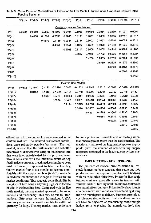
Table 3. Cross Equation Correlations of Errors for the Live Cattle Futures Prices / Variable Costs of CattleFeeding Systems

FP(t-1) FP(t-2) FP(t-3) FP(t-4) FP(t-5) FP(t-6) FP(t-7) FP(t-8) FP(t-9) FP(t-10) FP(t-11)

Contemporaneous Cost Models

FP(t) 0.6589 0.0550 -0.0609 0.1602 0.2194 0.1063 -0.0460 0.0864 0.2569 0.1031 0.0091

FP(t-1) 0.4436 0.1890 0.2558 0.3245 0.3150 0.2031 0.2688 0.3315 0.2381 0.1917

FP(t-2) 0.4610 -0.1136 0.0347 0.3734 0.3907 0.1652 -0.0504 0.0059 0.2611

FP(t-3) 0.4351 0.0551 0.1827 0.4588 0.4079 0.1660 0.1535 0.2543

FP(t-4) 0.6063 0.3112 0.3509 0.5005 0.4244 0.3164 0.1260

FP(t-5) 0.5687 0.4079 0.4792 0.5366 0.4664 0.2927

FP(t-6) 0.4280 0.2405 0.2563 0.2284 0.1958

FP(t-7) 0.6789 0.2309 0.1670 0.2960

FP(t-8) 0.6070 0.4184 0.3870

FP(t-9) 0.7865 0.4243

FP(t-10) 0.5453

Incurred Cost Models

FP(t) 0.5872 -0.2942 -0.4133 -0.2596 0.0053 -0.1731 -0.2143 -0.1015 -0.0018 -0.0628 -0.2593

FP(t-1) 0.3453 -0.1410 -0.1660 0.0101 0.0742 -0.0793 -0.1206 -0.0730 -0.0748 -0.1391

FP(t-2) 0.6907 0.2420 -0.0364 0.2917 0.2336 0.0505- -0.1000 -0.0610 0.0726

FP(t-3) 0.5634 0.0455 0.2051 0.3518 0.2744 0.0632 0.0767 0.1155

FP(t-4) 0.2124 0.0615 0.2768 0.4113 0.2024 0.0199 0.0087

FP(t-5) 0.5410 0.3307 0.4230 0.5063 0.4295 0.2481

FP(t-6) 0.4337 0.2393 0.2601 0.2235 0.1901

FP(t-7) 0.6851 0.2731 0.1945 0.3061

FP(t-8) 0.6321 0.4546 0.4077

FP(t-9) 0.8010 0.4945

FP(t-10) 0.5817

offered early in the contract life were reversed as the future supplies with variable cost of feeding infor-contract matured. The incurred cost system correla- mation to a greater extent than the cattle market. Thetions were primarily positive but small. The hog reactionary nature of the hog market appears appro-market, more so than the cattle market, did not offer priate given the absence of self-defeating supplyincentives or disincentives early in the contract life responses measured in the incurred cost system cor-that were later self-defeated by a supply response. relations.This is consistent with the inflexible nature of hogfeeding decisions once breeding decisions have been IMPLICATIONS FOR HEDGINGmade. However, it appeared to take the live hog The presence of rational price formation in live-futures market four to six months to become com- stock futures markets suggests that cattle and hogfortable with the supply numbers (initially available producers need to approach preplacement hedgingin bred sow intentions) and to begin to forecast future with realistic price objectives. Prices for live cattlemarket conditions. This suggests some flexibility in futures contracts generally move in tandem withslaughter of bred sows and young pigs, or in the use variable costs of feeding until the futures contract isof gilts in the breeding herd. Compared with the live two months from delivery. Prices for live hog futurescattle market, the hog market appeared to be more contracts move with variable costs of feeding duringnervous and reactionary. This may be due to infor- the fifth month prior to delivery but react strongly tomational differences between the markets. USDA cost changes at other times. If cattle and hog produc-inventory reports are released monthly for cattle but ers have an objective of establishing profit marginquarterly for hogs. The hog market must anticipate hedges prior to placing the animals on feed, they

244

Table 4. Cross Equation Correlations of Errors for the Live Hog Futures Prices / Variable Costs of HogFeeding Systems

FP(t-1) FP(t-2) FP(t-3) FP(t-4) FP(t-5) FP(t-6) FP(t-7) FP(t-8) FP(t-9) FP(t-10) FP(t-11)

Contemporaneous Cost Models

FP(t) 0.3941 0.1683 0.0754 -0.0387 -0.1360 -0.0847 -0.1408 -0.0573 -0.0470 -0.0743 0.0018

FP(t-1) 0.4959 0.3330 -0.0557 -0.1088 -0.2348 -0.2243 -0.1762 -0.0975 -0.0896 -0.0513

FP(t-2) 0.4850 0.1345 -0.0303 -0.0772 -0.1079 0.0114 -0.0579 -0.0240 0.0301

FP(t-3) 0.4250 0.2979 0.2351 0.1340 0.1869 0.1041 0.1395 0.2999

FP(t-4) 0.5238 0.3804 0.3030 0.2997 0.1851 0.2806 0.1816

FP(t-5) 0.5504 0.3301 0.3859 0.2904 0.3349 0.1944

FP(t-6) 0.6740 0.6546 0.5109 0.5045 0.3203

FP(t-7) 0.8650 0.8044 0.7192 0.5858

FP(t-8) 0.8140 0.7651 0.5549

FP(t-9) 0.7493 0.5965

FP(t-1 0) 0.6639

Incurred Cost Models

FP(t) 0.6586 0.4479 0.2253 0.0346 -0.0539 0.0456 0.0481 0.1240 0.1082 0.1034 0.0906

FP(t-1) 0.8292 0.6229 0.3104 -0.0324 -0.0290 -0.0252 0.0505 0.1013 0.0886 0.1222

FP(t-2) 0.7934 0.4903 -0.0082 0.0630 0.0228 0.1409 0.1228 0.1355 0.1540

FP(t-3) 0.6377 0.1513 0.1615 0.0952 0.1562 0.0978 0.1450 0.2793

FP(t-4) 0.3728 0.2529 0.1758 0.2579 0.1891 0.2809 0.2333

FP(t-5) 0.5545 0.3377 0.3890 0.2976 0.3410 0.1948

FP(t-6) 0.6962 0.6688 0.5266 0.5169 0.3238

FP(t-7) 0.8555 0.7890 0.7108 0.5740

FP(t-8) 0.8267 0.7797 0.5628

FP(t-9) 0.7667 0.6131

FP(t-10) 0.6710

cannot expect to hedge substantially above variable probability of observing live cattle futures trading atfeeding costs. Figures 2 and 3 are histograms of the a $2/cwt. or greater discount under USDA feedingprobability of observing specific differences ($/cwt.) budget figures during the placement period is lessbetween futures prices and USDA variable costs of than 2 percent. However, during the delivery month,feeding. Figure 2 presents, for cattle, the probability futures have been $2/cwt. or more under incurredof differences between costs five months from deliv- costs 23 percent of the time." The same phenomenaery and futures five months from delivery, and be- hold for higher prices. Futures prices during thetween costs five months from delivery and futures in placement month have traded in excess of $4/cwt.the delivery month. The histograms were con- above USDA feeding costs approximately 12 per-structed using two dollar-per-hundredweight inter- cent of the time. However, during delivery monthsvals; the midpoints of the intervals are indicated on futures have been in excess of incurred costs bythe horizontal figure axes. $4/cwt. for approximately 40 percent of the time.

The probability of observing large positive or A similar pattern is revealed for hogs in Figure 3.negative differences between futures prices and Large positive or negative differences between fu-feeding costs incurred at placement was greater for tures prices and actual hog feeding costs were morethe delivery month futures prices than for placement likely to be observed in the delivery month than inmonth futures prices. For example, in Figure 2, the the placement month. Futures prices have not been

Interval probabilities in the histogram were cumulated for this interpretation.

245

Probability35% -

30c

.. ......... . . .. I30%

25%

20%

15%

10%

0%

-13 -11 -9 -7 -5 -3 -1 l 3 5 7 9 11 13 15 17 19

Futures less Costs a: Placement ($/cwt.)

I[3 Futures at Delivery M Futures at Placer-ent

Figure 2. Histograms of the Difference Between Live Cattle Futures at Delivery and USDA Great Plains Cat-tle Feeding Costs at Placement and of the Difference Between Live Cattle Futures at Placementand USDA Great Plains Cattle Feeding Costs at Placement.

observed below USDA variable feeding costs five variable costs by hedging prior to placement. This ismonths prior to delivery. However, during the deliv- the standard risk/return tradeoff of portfolio theory.ery month futures' have been observed below the Thus, the crucial observation is that the produceractual feeding costs 10 percent of the time. Likewise, who hedges at or before placement can reduce thefutures prices have been observed in excess of feed- probability of losses, but very profitable returns areing costs by $14/cwt. only 1 percent of the time also eliminated.during the placement month. However, during thedelivery month, this difference has been observed 25 CONCLUSIONSpercent of the time. Rational price formation is generally supported by

Caution should be used in interpreting the level of the behavior of distant live cattle and live hog futuresthe difference between futures prices and USDA prices. Distant futures contracts trade at pricesaverage variable feeding costs as profits or, more around the average costs of feeding during the timeaccurately, as returns to fixed costs. The magnitudes period when a supply response is possible. However,may be biased upward, as USDA costs have been after feeding commitments are made, market pricesfound to be higher than industry costs (Trapp). Fur- likely adjust to reflect expected market conditions asther, the futures price must be adjusted for basis to those conditions become known. As a result, live-obtain a cash price. The issue at hand is the wide stock futures markets forecast poorly at longer timespread between futures prices and cost at the time of horizons and improve as the contract nears maturity.delivery and the narrow spread during the placement Evidence of rational price formation suggests that anmonths. Bias in returns to fixed costs will not affect analytical framework which attempts to draw marketthe spreads observed. Therefore, if a cattle feedlot efficiency conclusions based solely on forecast per-operator's feeding costs are consistently $2/cwt. formance is too stringent because, it ignores thelower than the USDA feeding budget, then it appears arbitrage between futures markets and feeding deci-that the producer can establish a price, by hedging sions.prior to placement, covering feeding costs more than The live cattle futures market exhibits rational97 percent of the time. However, 88 percent of the price formation to a greater degree than does the livetime the feeder will earn less than $4/cwt. above hog futures market. This may be due to the level of

246

.......... .... ..~~~~~~~~~~~~~~~~~~~~~~~~~~~~~~~~~~~~~~~~~~~~~~~~~~~~~~~~~~~~~~~~~~~~~~~~~~~~~~~~~~~~~~~~~~~~~~~~~~~~~~~~~~~~~~~~~~~~~~~~~~~~~~~~~~~~~~~~~~~~~~~~~~~~~~~~~~~~~~~~~~~~~~~~~~~~~~~o~~~~~~~~~~~~~~~~~~..... ..... ....... .......~ ~ ~~ ~ ~ ~~~~~~~~i........i.................... ....

Probability25%

'.." . . ...... .....

OA i I X ' i -'": ' : ^ '~ I

-11 -9 -7 -5 -3 -1 1 3 5 7 9 111315 17 19 21 23 25 27Futures less Costs at Placement ($/cwt.)

'i"I Futures at Delivery m Futures at Placement

Figure 3. Histograms of the Difference Between Live Hog Futures at Delivery and USDA Corn Belt HogFeeding Costs at Placement and of the Difference Between Live Hog Futures at Placement andUSDA Corn Belt Hog Feeding Costs at Placement.

uncertainty in the respective production processes. hedger will effectively manage costs and establishIn the hog market, there is more supply uncertainty hedges when futures prices offer costs plus a reason-because government reports are less frequent. Also, able rate of return. Rational price formation limitshog production may be more uncertain as it may be the futures market from offering significant profitsmore influenced by weather, disease, birth rates, and during the phase of a contract's life when futureother factors. For live cattle, the decision most affect- supplies can still be influenced. The market does noting rational price formation is whether animals are offer significant losses during this time period either.finished or left in backgrounding programs. This Beyond the period when a supply response can oc-difference between live cattle and live hog futures cur, more profitable hedging opportunities may arisemarkets appears to merit further investigation, and a more selective approach to hedging may yield

From the viewpoint of the decision maker inter- higher returns. However, the higher returns are of-ested in using live cattle or hog futures markets to fered only in exchange for the higher level of riskmanage price risk, the results have implications for associated with having unhedged production afterhedging strategy selection as well as for identifying the supply response period, where there is potentialthe type of producer who can use futures to hedge for price decreases as the market accumulates infor-effectively. The results suggest that the successful mation.

REFERENCES

Breusch, T. S., and A. R. Pagan. "The Lagrange Multiplier Test and its Applications to Model Specificationsin Econometrics." Rev. Econ. Studies ,47 (1980):239-253.

Coiling, P. L., and S. H. Irwin. "On the Reaction of Live Hog Futures Prices to Informational Components inQuarterly USDA Hogs and Pigs Reports." Proceedings of the 1989 NCR-134 Conference on CommodityPriceAnalysis, Forecasting, andMarket RiskManagement, pp. 17-35. Dep. Econ., Iowa State University,1989.

Coiling, P. L., and S. H. Irwin. "The Reaction of Live Hog Futures Prices to USDA Hogs and Pigs Reports."Am. J. Agr. Econ., 72(1990):84-94.

247

Cox, D. R., and D. J. Hinkley. Theoretical Statistics. London: Chapman and Hall, 1974.Dewbre, J. H. "Interrelationships Between Spot and Futures Markets: Some Implications of Rational

Expectations." Am. J. Agr. Econ., 63(1981):926-933.Ehrich, R. L. "Cash-Futures Price Relationships for Live Beef Cattle." Am. J. Agr. Econ., 51(1969):26-40.Fama, E. F. "Efficient Capital Markets: A Review of Theory and Empirical Work." J. Finance, 25(1970):383-

417.Garcia, P., M. A. Hudson, and M. E. Waller. "The Pricing Efficiency of Agricultural Futures Markets: An

Analysis of Previous Research Results." So. J. Agr. Econ., 20(1988a):119-130.Garcia, P., R. M. Leuthold, T. R. Fortenbery, and G. F. Sarassoro. "Pricing Efficiency in the Live Cattle Futures

Market: Further Interpretation and Measurement." Am. J. Agr. Econ., 70(1988b): 162-169.Gray, R. "The Futures Market for Maine Potatoes: An Appraisal."Vol. 3, Selected Writings on Futures

Markets, A.E. Peck, ed. Chicago: Chicago Board of Trade, 1977.Harvey, A. C. Time Series Models. Oxford: Philip Allan, 1981.Helmuth, J. W. "A Report on the Systematic Downward Bias in Live Cattle Futures Prices." J. Futures

Markets, 1(1981):347-358.Hoffman, G. "The Effects of Futures Prices on Short-Run Supply of Fed Cattle and Hogs." Livestock Futures

Research Symposium, R. M. Leuthold and P. Dixon, eds. Chicago: Chicago Mercantile Exchange, 1979.Hudson, M. A., S. R. Koontz, and W. D. Purcell. "The Impact of Quarterly Hogs and Pigs Reports on Live

Hog Futures Prices: An Event Study of Market Efficiency." Dep. Agri. Econ. Bull. AE-54, VirginiaPolytechnic Institute and State University, June 1984.

Just, R. E., and G. C. Rausser. "Commodity Price Forecasting with Large-Scale Econometric Models and theFutures Markets." Am. J. Agr Econ., 63(1981): 197-208.

Kamara, A. "Issues in Futures Markets: A Survey." J. Futures Markets, 2(1982):261-294.Kiviet, J. "On the Rigor of Some Specification Tests in Modelling Pyramidic Relationships." Rev. Econ.

Studies, 53(1986):241-262.Koontz, S.R., M. A. Hudson, and M. W. Hughes. "Rational Price Formation in Live Cattle and Live Hog

Futures Markets." Oklahoma Agricultural Experiment Station Technical Bulletin, Oklahoma StateUniversity, forthcoming.

Leuthold, R. M. "The Price Performance on the Futures Market of a Nonstorable Commodity: Live BeefCattle." Am. J. Agr. Econ., 56(1974):271-279.

Leuthold, R. M., and P. Hartmann. "A Semi-Strong Form Evaluation of the Efficiency of the Hog FuturesMarket." Am. J. Agr. Econ., 63(1979):482-489.

Leuthold, R. M., P. Garcia, B. D. Adam, and W. I. Park. "The Necessary and Sufficient Conditions for MarketEfficiency: The Case of Hogs." Appl. Econ., 21(1989): 193-204.

Martin, L., and P. Garcia. "The Price-Forecasting Performance of Futures Markets for Live Cattle and Hogs:A Disaggregate Analysis." Am. J. Agr. Econ., 63(1981):209-215.

Miller, S. E. "The Response of Futures Prices to New Market Information: The Case of Live Hogs." So. J.Agr. Econ., 2(1979):67-70.

Miller, S. E., and D. E. Kenyon. "Empirical Analysis of Live-Hog Futures Price Use by Feeders and Packers."Livestock Futures Research Symposium, R. M. Leuthold and P. Dixon, eds. Chicago: Chicago MercantileExchange, 1979.

Miller, S. E., and D. E. Kenyon. "Rational Price Formation in the Fed Cattle Futures Market." Staff Paper,SP-77-7, Virginia Polytechnic Institute and State University, Department of Agricultural Economics,March 1977.

Paul, A. P., and W. T. Wesson. "Pricing Feedlot Services Through Futures." Agr: Econ. Res., 19(1967):35-45.Peck, A. E. "The Economic Role of Traditional Commodity Futures Markets." Futures Markets: Their

Economic Role, A. E. Peck, ed. Washington D. C.: American Enterprise Institute for Public PolicyResearch, 1985.

Peck, A. E. "Futures Markets and Intertemporal Commodity Pricing." Efficiency in Agricultural and FoodMarketing, R. L. Kilmer and W. J. Armbruster, eds. Ames, Iowa: Iowa State University Press, 1987.

248

Purcell, W. D., and M. A. Hudson. "The Economics Roles and Implications of Trade in Livestock Futures."Futures Markets: Regulatory Issues, A. E. Peck, ed. Washington, D. C.: American Enterprise Institutefor Public Policy Research, 1985.

Purcell, W. D., D. Flood, and J. S. Plaxico. "Cash-Futures Interrelationships in Live Cattle: Causality,Variability, and Pricing Processes." Livestock Futures Research Symposium, R. M. Leuthold and P.Dixon, eds. Chicago: Chicago Mercantile Exchange, 1979.

Schroeder, T., J. Blair, J. Mintert, and A. Featherstone. "The Impacts of USDA Inventory Reports on LivestockCash and Futures Prices." Proceedings of the 1989 NCR-134 Conference on Commodity Price Analysis,Forecasting, and Market Risk Management, pp. 36-52. Dep. Econ., Iowa State University, 1989.

Shonkwiler, J.S. "Are Livestock Futures Prices Rational Forecasts?" West. J. Agr. Econ., 11(1986):123-128.

Stein, J. L. "Speculative Price: Economic Welfare and the Idiot of Chance." Rev. Econ. Stat., 63(1981):223-232.

Tomek, W. G., and R. W. Gray. "Temporal Relationships Among Prices on Commodity Futures Markets:Their Allocative and Stabilizing Roles." Am. J. Agr. Econ., 52(1970):372-380.

Trapp, J. N. "Seasonal Aspects of Cattle Feeding Profits." Oklahoma Agricultural Experiment Station,Oklahoma State University, Department of Agricultural Economics, Current Farm Economics,62(1989):19-30.

Working, H. "Theory of the Inverse Carrying Charge in Futures Markets." J. Farm Econ., 30(1948):1-28.

249

250