?lj ;: . ,./ leading edge vortex dynamics on a … · /?lj ;:_. t ,_,,. / #i_ 13 leading edge...
TRANSCRIPT

t , //?lJ ;:_. ,_ ,.
#I_ 13
LEADING EDGE VORTEX DYNAMICS
ON A PITCHING DELTA WING
Scott P. LeMay, Stephen M. Batill, and Robert C. Nelson
University of Notre Dame
(X'A':,',-L.'.-! i,'_ _27) LFA!-_ING _hC, f V_J_',T" x
T_,,=si'._ (:*,'_,t.r_:, '-_m_, 'drily.) i. 75 p CSCL F)I Adncl _s
NAG-I-727
April 1988
https://ntrs.nasa.gov/search.jsp?R=19900009882 2018-05-28T22:01:20+00:00Z

LEADING EDGE VORTEX DYNAMICS
ON A PITCHING DELTA WING
A Thesis
Submitted to the Graduate School
of the University of Notre Dame
in Partial Fulfillment of the Requirements
for the Degree of
Master of Science
by
Scott P. LeMay, B.S.A.E.
Co-Director
Co-Director
Department of Aerospace and Mechanical Engineering
Notre Dame, Indiana
April, 198%
LEADING EDGE VORTEX DYNAMICS
ON A PITCHING DELTA WING
Abstract
by
Scott P. LeMay
The reading edge flow structure was investigated on a 70 ° flat plate detta
wing which was pitched about its 1/2 chord position, to increase understanding
of the high angle of attack aerodynamics on an unsteady delta wing. The wing
was sinusoidally pitched at reduced frequencies ranging from k - 2_fc/u = 0.05
to 0.30 at chord Reynolds numbers between 90,000 and 350,000, for angle of
attack ranges of e_= 29 ° to 390 and e_= 0° to 45 °. The wing was also
impulsively pitched at an approximate rate of 0.7 rad/s. Dunng these dynamic
motions, visualization of the leading edge vorticies was obtained by entraining
titanium tetrachloride into the flow at the model apex.
The location of vortex breakdown was recorded using 16ram high speed
motion picture photography. When the wing was sinusoidally pitched, a
hysteresis was observed in the location of breakdown position. This hysteresis
increased with reduced frequency. The velocity of breakdown propagation
along the wing, and the phase lag between model motion and breakdown
location were also determined. When the wing was impulsively pitched, several
convective times were required for the vortex flow to reach a steady state.
Detailed information was also obtained on the oscillation of breakdown position
in both static and dynamic cases.

DEDICATION
This work is dedicated to my parents, Robert P. LeMay and Edna M.
LeMay, and also my brother Jeffery P. LeMay. Their love, support, and
encouragement made it possible.
ii

TABLE OF CONTENTS
Page
LIST OF TABLES .............................................................................................................. v
LIST OF FIGURES ........................................................................................................... vi
NOMENCLATURE .......................................................................................................... xii
ACKNOWLEDGEMENTS ............................................................................................. xiv
INTRODUCTION .................................................................................................. 1
1.1 Perspective .................................................................................................... 11.2 Background Study ....................................................................................... 3
1.2.1 The Leading Edge Vortex and Vortex Breakdown ................. 31.2.2 Unsteady Vortex Dynamics ......................................................... 4
The Effect of Pitching ................................................................... 5The Effect of Plunging ................................................................. 8The Effect of Unsteady Freestream Flow ............................... 10
Static Hysteresis ....................................................................... 101.2.3 Brief Summary of Unsteady Work Reviewed ........................ 11
1.3 Scope of Work ............................................................................................ 12
II. EXPERIMENTAL APPARATUS ....................................................................... 1 5
2.1 Wind Tunnel ................................................................................................ 152.2 Model ............................................................................................................ 16
2.3 Unsteady Pitching Mechanism ................................................................ 172.4 Flow Visualization ...................................................................................... 18
2.5 Photographic Records ............................................................................... 232.6 Hotwire Anemometry ................................................................................. 24
2.7 Displacement Transducer ........................................................................ 252.8 Data Acquisition Systems ......................................................................... 27
II1. PROCEDURE AND DATA ACQUISITION ..................................................... 28
3.1 Model Motion .............................................................................................. 28
3.2 Freestream Response ............................................................................... 29
3.3 High Speed Motion Picture Data ............................................................ 303.4 35ram Photographic Data ......................................................................... 313.5 Reduction of Photographic Data ............................................................. 32
3.5.1 Wayne-George Optical Comparator ........................................ 32
3.5.2 Wayne-George to DEC Interface ............................................ 33
iii

iv
3.5.3 Wayne George Accuracy ........................................................... 343.5.4 Data Acquisition with the Wayne-George .............................. 353.5.5 Accuracy of Reduced Data ........................................................ 39
IV. RESULTS ............................................................................................................ 43
4.1 Introduction .................................................................................................. 434.2 Model Motion .............................................................................................. 45
4.3 Freestream Response ............................................................................... 464.4 Vortex Breakdown over a Static Wing .................................................... 494,5 Vortex Breakdown Dynamics using High Speed Cinema ................. 50
4.5.1 General Description of Vortex Flow Response ..................... 514.5.2 x/c vs Angle of Attack .................................................................. 524.5.3 Width of the Hysteresis Loop .................................................... 554.5.4 Phase Difference between Breakdown Location and
Model Motion ........................................................................ 57
Propagation Velocity of Breakdown Location ...................... 59Oscillation of Breakdown Position ........................................... 61
Vortex Core Inclination Angle ................................................... 63Large Amplitude Oscillations .................................................... 64Impulsive Change in Angle of Attack ...................................... 68
Vortex Breakdown Dynamics using 35mm Photography ................... 69
4.5.54,5,64.5.74.5.84.5.9
4.6
V. CONCLUSIONS AND RECOMMENDATIONS ............................................ 71
5.1 Conclusions ................................................................................................ 725,2 Recommendations ..................................................................................... 75
FIGURES ......................................................................................................................... 78
APPENDIX A: Discrete Fourier Transforms of Model Motion ............................. 133
APPENDIX B: Freestream Velocity Fluctuation and Model Position ................. 140
APPENDIX C: Chordwise Breakdown Location and Model Position ............... 147
REFERENCES ............................................................................................................. 158

LIST OF TABLES
Table Page
4.2
4.3
4.4
4.5
Digitized High Speed Movie Cases ............................................................40
Harmonic Distortion in the Sinusoidal Pitching Motion of theDelta Wing Model ..................................................................................46
Response of the Freesteam Flow due to the Varying TunnelBlockage Caused by the Oscillating Model ......................................48
Cases for which the Reynolds Number was Constant and theReduced Frequency Varied. Angle of Attack Range = 290 to39° ............................................................................................................52
Cases for which the Reduced Frequency was Constant and theReynolds Number Varied. Angle of Attack Range = 29° to39° ............................................................................................................54
Average rms of Breakdown Location during Oscillatory Pitching..........62
V

LIST OF FIGURES
Figure
1.1
1.2
2.1
2.2
2.3
2.4
2.5
2.6
2.7
2.8
2.9
2.10
2.11
2.12
3.1
3.2
3.3
3.4
3.5
3.6
3.7
Page
Vortex Flow over a Delta Wing ..................................................................... 78
Schematic of Leading Edge Flow Patterns ................................................ 79
Wind Tunnel Facility ....................................................................................... 80
Delta Wing Model ........................................................................................... 81
Operating Range of Test Facility .................................................................. 82
Schematic of Delta Wing Pitching Mechanism ......................................... 83
Schematic of Pitching Mechanism Control Box ........................................ 84
Kerosene Smoke Generator ......................................................................... 85
Smoke Rake .................................................................................................... 86
Kerosene Smoke Filaments Impinging Model Apex ................................ 87
Titanium Tetrachloride Injection System .................................................... 88
16 mm Motion Picture Camera Setup ......................................................... 89
35mm SLR Camera Setup ............................................................................ 90
Linear Variable Differential Transformer Schematic ................................ 91
Example of a Photographic Image obtained from a Side View ............. 92
Schematic of Photographic Image obtained from a Side View ............. 92
Wayne-George Optical Comparator Configuration .................................. 93
Example of a Photographic Image obtained from a Top View ............... 94
Schematic of Photographic Image obtained from a Top View ............... 94
Representative Plot Illustrating how Angle of Attack Variesbetween Pitching Cycles at Specific Points within the Cycle ................. 95
Representative Plot Illustrating how the Chordwise BreakdownLocation Varies between Pitching Cycles at Specific Pointswithin the Cycle ............................................................................................... 96
vi

4.1
4.2
4.3a
4.3b
4.4
4.5a
4.5b
4.6
4.7a-j
4.8a
4.8b
4.8c
4.8d
vii
Attachment of LVDT to Delta Wing Pitching Mechanism ......................... 97
LVDT Calibration Curve, 29 ° to 38 ° ............................................................ 98
One Data Record of the Freesteam Response due to ModelMotion for a Representative Case ............................................................... 99
Ensemble Average of 100 Data Records of the FreestreamResponse due to Model Motion for a Representative Case ................... 99
Static Chordwise Location of Vortex Breakdown for Increasing
and Decreasing Angle of Attack. Angle of Attack Range = 29 ° to39 °, U = 30 ft/s, Re = 260,000 ..................................................................... 100
Discrete Fourier Transform of the Variation in Chordwise
Breakdown Location from Mean Position at an Angle of Attackof 29 °. U = 30 if/s, Re ---260,000 ............................................................... 101
Discrete Fourier Transform of the Variation in Chordwise
Breakdown Location from Mean Position at an Angle of Attackof 39 °. U = 30 ft/s, Re = 260,000 ................................................................ 101
RMS of the Chordwise Breakdown Location at Static Angles ofAttack throughout the Range of Pitching Motion. Angle of AttackRange = 29 ° to 39 °, U = 30 ft/s, Re = 260,000 ......................................... 102
Sequence of Photographs made from 16mm Movie Film whichIllustrates how the Chordwise Breakdown Location Varies
throughout a Pitching Cycle. Angle of Attack Range = 29 ° to 390 ...... 103
Chordwise Position of Vortex Breakdown during OscillatoryMotion. Angle of Attack Range = 29 ° to 39 °, k = 0.05, U = 30 ft/s,Re - 260,000 ................................................................................................. 104
Chordwise Position of Vortex Breakdown during Oscillatory
Motion. Angle of Attack Range -- 29 ° to 39 °, k = 0.10, U -- 30 ft/s,Re = 260,000 ................................................................................................. 105
Chordwise Position of Vortex Breakdown during Oscillatory
Motion. Angle of Attack Range = 29 ° to 39 °, k -- 0.20, U --- 30 ft/s,Re = 260,000 ................................................................................................. 106
Chordwise Position 'of Vortex Breakdown during Oscillatory
Motion. Angle of Attack Range = 29 o to 39 °, k -- 0.30, U -- 30 ft/s,Re = 260,000 ................................................................................................. 10 7

4.9a
4.9b
4.9c
4.10a
4.10b
4.11
4.12
4.13
4.14
4.15
4.16
viii
Chordwise Position of Vortex Breakdown during OscillatoryMotion. Angle of Attack Range = 29° to 39°, k = 0.20, U = 10 and20 if/s, Re = 90,000 and 175,000 .............................................................. 108
Chordwise Position of Vortex Breakdown during OscillatoryMotion. Angle of Attack Range = 29 ° to 39 °, k = 0.20, U = 30 and40 ft/s, Re - 260,000 and 350,000 ............................................................ 109
Chordwise Position of Vortex Breakdown during OscillatoryMotion. Angle of Attack Range = 29 ° to 39 °, k = 0.20, U = 10, 20,30, and 40 ft/s, Re = 90,000, 175,000, 260,000, and 350,000 ............ 11 0
Width of the Hysteresis Loops, presented in Figures 4.8a-d, overthe Angle of Attack Range of 29 ° to 39 ° for Reduced Frequenciesof k = 0.05, 0.10, 0.20, 0.30. U - 30 ft/s, Re = 260,000 .......................... 111
Width of the Hysteresis Loops, presented in Figures 4.9a-c, overthe Angle of Attack Range of 29 ° to 39 ° for Reynolds Numbers ofRe = 90,000, 175,000, 260,000, and 350,000. k = 0.20,U = 10, 20, 30, and 40 ft/s ............................................................................ 111
Representative Plot of Chordwise Breakdown Location andModel Angular Position as a Function of Period ..................................... 11 2
Phase Lag of the Vortex Flow as a Function of ReducedFrequency for a Reynolds Number of 260,000. Angle of AttackRange -- 29 ° to 39°,U = 30 ft/s ................................................................... 11 3
Phase Lag of the Vortex Flow as a Function of Reynolds Numberfor a Reduced Frequency of 0.20. Angle of Attack Range - 29 ° to39 ° ................................................................................................................... 11 3
Phase Lag of the Vortex Flow as a Function of PitchingFrequency for a Reynolds Number of 260,000 and a ReducedFrequency of 0.20. Angle of Attack Range -- 29 ° to 39 ° ....................... 11 4
Breakdown Propagation Velocity relative to the Delta Wingthroughout a Pitching Cycle for Reduced Frequencies ofk= 0.05, 0.10, 0.20, and 0.30. Angle of Attack Range = 29 ° to39 °, U = 30 ft/s, Re = 260,000 ..................................................................... 115
Breakdown Propagation Velocity relative to the Delta Wingthroughout a Pitching Cycle for Reynolds Numbers of 90,000,175,000,260,000, and 350,000. Angle of Attack Range - 29 ° to39 °, k = 0.20, U = 10, 20, 30, and 40 ftJs .................................................. 11 6

4.17
4.18
4.19a
4.19b
4.20a
4.20b
4.21
4.22
4.23
4.24
4.25a-j
ix
Reduced Breakdown Propagation Velocity relative to the Delta
Wing throughout a Pitching Cycle for Reduced Frequencies ofk -- 0.05, 0.10, 0.20, and 0.30. Angle of Attack Range - 29 ° to39 °, U = 30 ft/s, Re = 260,000 ..................................................................... 11 7
Reduced Breakdown Propagation Velocity relative to the DeltaWing throughout a Pitching Cycle for Reynolds Numbers of90,000, 175,000,260,000, and 350,000. Angle of Attack Range= 29 ° to 39 °, k = 0.20, U = 10, 20, 30, and 40 ft/s ................................... 11 8
RMS of the Chordwise Breakdown Location at Various Angles of
Attack throughout a Pitching Cycle. Angle of Attack Range = 29 °to 39 °, k -- 0.20, U = 30 ft/s, Re = 260,000 ................................................ 11 9
RMS of the Chordwise Breakdown Location at Various Angles of
Attack throughout a Pitching Cycle. Angle of Attack Range = 29 °to 39 °, k -- 0.20, U - 20 ft/s, Re = 175,000 ................................................ 119
Photograph used to Demonstrate that the Vortex Core can beAssumed to be Straight. Angle of Attack ~ 29 °, U = 30 ft/s,Re = 260,000 ................................................................................................. 120
Photograph used to Demonstrate that the Vortex Core can beAssumed to be Straight. Angle of Attack -- 39 °, U = 30 ft/s,Re -- 260,000 ................................................................................................. 1 20
Vortex Core Inclination Angle during Oscillatory Motion. Angle ofAttack Range = 29 ° to 39 °, k = 0.05 and 0.10, U = 30 ft/s,Re = 260,000 ................................................................................................. 121
Vortex Core Inclination Angle during Oscillatory Motion. Angle ofAttack Range = 29 ° to 39 °, k = 0.20 and 0.30, U = 30 ft/s,Re - 260,000 ................................................................................................. 122
Vortex Core Inclination Angle during Oscillatory Motion. Angle ofAttack Range - 29 ° to 39 °, k -- 0.20, U -- 10 and 20 ft/s,Re -- 90,000 and 175,000 ............................................................................ 123
Vortex Core Inclination Angle during Oscillatory Motion. Angle of
Attack Range = 29 ° to 39 °, k = 0.20, U = 30 and 40 ft/s,Re -- 260,000 and 350,000 ......................................................................... 124
Sequence of Photographs made from 16mm Movie Film whichIllustrates how the Chordwise Breakdown Location Varies
throughout a Pitching Cycle. Angle of Attack Range = 0° to 45 °,k = 0.30, U -- 30 fts, Re = 260,000 .............................................................. 125

4.26a-j
4.27a
4.27b
4.28
4.29a
4.29b
4.30
A1
A2
A3
A4
A5
A6
B1
X
Sequence of Photographs made from 16mm Movie Film whichIllustrates the Separation and Reattachment Processes of theVortex Flow .................................................................................................. 126
Chordwise Position of Vortex Breakdown during OscillatoryMotion. Angle of Attack Range - 0 ° to 45 °, k = 0.05 and 0.30,U = 30 ft/s, Re = 260,000 ............................................................................. 127
Chordwise Position of Vortex Breakdown during OscillatoryMotion for a Large and Small Amplitude Case, and Static Data.Angle of Attack Range = 0° to 45 ° and 29 ° to 39 °, k = 0.30,U = 30 ft/s, Re = 260,000 ............................................................................. 128
Vortex Core Inclination Angle during Oscillatory Motion. Angle ofAttack Range -- 0 ° to 45 °, k = 0.05 and 0.30, U = 30 ft/s,Re = 260,000 ................................................................................................. 129
Response of the Chordwise Breakdown Location due to an
Impulsive Pitch-up in Angle of Attack. Angle of AttackRange = 28 ° to 37 °, k = 0.45, U = 30 ft/s, Re -- 260,000 ......................... 130
Response of the Chordwise Breakdown Location due to an
Impulsive Pitch-down in Angle of Attack. Angle of AttackRange = 28°to 37 °, k = 0.45, U = 30 ft/s, Re = 260,000 ......................... 131
Spanwise Position of Vortex Breakdown during OscillatoryMotion. Angle of Attack Range = 29 ° to 39% k -- 0.05, 0.20 and0.30, U - 30 if/s, Re -- 260,000 ................................................................... 132
DFT of Model Motion. Angle of Attack Range = 29 ° to 39 °,k = 0.05, U = 30 ft/s ....................................................................................... 134
DFT of Model Motion. Angle of Attack Range = 29 ° to 39 °,k - 0.30 U - 30 ft/s ....................................................................................... 135
DFT of Model Motion. Angle of Attack Range = 29 ° to 39 °,k = 0.20 U = 10 ft/s ....................................................................................... 136
DFT of Model Motion. Angle of Attack Range = 29 ° to 39 °,k -- 0.20 U -- 40 ft/s ....................................................................................... 137
DFT of Model Motion. Angle of Attack Range = 0 ° to 45 °,k -- 0.05 U -- 30 ft/s ....................................................................................... 138
DFT of Model Motion. Angle of Attack Range -- 0 ° to 45 °,k = 0.30 U = 30 ft/s ....................................................................................... 139
Freestream Velocity Fluctuation and Model Position. Angle ofAttack Range = 29 ° to 39% k -- 0.05, U = 30 ft/s ....................................... 141
B2
B3
B4
B5
B6
C1
C2
C3
C4
C5
C6
C7
C8
C9
C10
xi
Freestream Velocity Fluctuation and Model Position. Angle ofAttack Range = 29° to 39°, k = 0.05, U = 30 ft/s .......................................142
Freestream Velocity Fluctuation and Model Position. Angle ofAttack Range = 29° to 39°, k = 0.20, U = 10 ft/s .......................................143
Freestream Velocity Fluctuation and Model Position. Angle ofAttack Range = 29 ° to 39 °, k = 0.20, U = 40 ft/s ....................................... 144
Freestream Velocity Fluctuation and Model Position. Angle ofAttack Range = 0 ° to 45 °, k = 0.05, U = 30 ft/s ......................................... 145
Freestream Velocity Fluctuation and Model Position. Angle ofAttack Range = 0 ° to 45 °, k = 0.30, U = 30 ft/s ......................................... 146
Chordwise Breakdown Location and Model Position. Angle ofAttack Range -- 29 ° to 39 °, k = 0.05, U = 30 ft/s, Re --!-260,000 ............ 148
Chordwise Breakdown Location and Model Position. Angle ofAttack Range = 29 ° to 39 °, k = 0.10, U = 30 ft/s, Re = 260,000 ............ 149
Chordwise Breakdown Location and Model Position. Angle ofAttack Range = 29 ° to 39 °, k = 0.20, U = 30 ft/s, Re = 260,000 ............ 150
Chordwise Breakdown Location and Model Position. Angle ofAttack Range = 29 ° to 39 °, k = 0.30, U = 30 ft/s, Re = 260,000 ............ 151
Chordwise Breakdown Location and Model Position. Angle ofAttack Range = 29 ° to 39 °, k = 0.20, U = 10 ft/s, Re = 90,000 .............. 152
Chordwise Breakdown Location and Model Position. Angle ofAttack Range -- 29 ° to 39 °, k = 0.20 U = 20 ft/s, Re = 175,000 ............ 153
Chordwise Breakdown Location and Model Position. Angle ofAttack Range = 29 ° to 39 °, k = 0.20 U = 30 ft/s, Re = 260,000 ............ 154
Chordwise Breakdown Location and Model Position. Angle ofAttack Range = 29 ° to 39 °, k = 0.20 U = 40 ft/s, Re - 350,000 ............ 155
Chordwise Breakdown Location and Model Position. Angle ofAttack Range = 0° to 45 °, k -- 0.05, U = 30 ft/s, Re = 260,000 .............. 156
Chordwise Breakdown Location and Model Position. Angle ofAttack Range = 0 ° to 45 °, k = 0.30, U - 30 ft/s, Re = 260,000 .............. 157

NOMENCLATURE
Symbols
C
f
g
k
K
Re
s
t
T
U
U
X
Y
O_
&
1.)
C0
Root chord length
Pitching frequency
Gravitational constant
2_fcReduced frequency,
Nondimensional pitch rate,
ucReynolds number, m
13
Local semi-span
Time (seconds)
Dimensionless time,t
m
Freestream Velocity
Freestream Velocity
Distance from apex parallel with wing chord
Distance from root chord parallel to trailing edge
Angle of Attack (degrees)
Pitch rate (radians/second)
Vortex core inclination angle (degrees)
u
Reduced Velocity, _"c
Convective time unit, _- (seconds)
Kinematic viscosity of air
Angular Velocity
xii

xiii
LVDT
DFT
rms
SCR
SLR
TiCI4
Linear Variable Differential Transformer
Discrete Fourier Transform
Root mean square
Silicon Controlled Rectifier
Single Lens Reflex
Titanium tetrachloride

ACKNOWLEDGEMENTS
The author would like to acknowledge and thank the following personsfor their help, advice, and contributions:
Dr. Stephen M. Batill and Dr. Robert C. Nelson, faculty advisors, for theirguidance and recommendations which have been instrumental in thisresearch.
Roger Davis, for the time he spent machining and fabricating theunsteady pitching mechanism and for his advice in the design.
Joe Hollkamp, Mike Brendel, and Thom Bradley, for their advice in thedata collection and reduction, and for their help with the Aero Labcomputing systems in general.
Dr. Ng and Dr. Gad-eI-Hak, for their suggestions made during the writingof this thesis.
Mike Swadner, for the construction of experimental equipment and theadvice he offered, and to Roger Kenna for his help with development ofphotographic data.
The work was sponsored by the NASA Langley Research CenterNAG-I-727, and the University of Notre Dame.
xiv

CHAPTER I
INTRODUCTION
1.1 Perspective
Over the past few decades, the flow over a steady delta wing has been
studied extensively. At low angles of attack, the flow is attached to the top and
bottom surfaces of the wing, and lift is produced in the same manner as on a
conventional airfoil. At moderate angles of attack, the flow separates from the
leading edge of the wing to form two counter- rotating vortices. It is these
separated vortices, rather than attached flow, which are responsible for
producing lift. The lift increases non-linearly with angle of attack to a maximum
value, and then tapers off slowly. At the higher angles of attack, a phenomenon
known as vortex breakdown occurs, in which the vortex flow undergoes a
sudden transformation. This breakdown appears first in the wake, and then with
increasing angle of attack the breakdown location moves upstream and
eventually above the top surface of the wing. If vortex breakdown occurs over
the top surface of wing, the large suction pressures which are associated with
the leading edge vortices are reduced. This results in a loss of lift and a change
in the pitching moment.
Most of our modern military aircrafts (which possess delta wings), go
through many dynamic motions from takeoff through landing. These dynamic
motions occur especially in dogfight situations, where an aircraft is

_ 2
maneuvering and changing speeds almost constantly. Future aircraft may be
required to operate at angles of attack beyond static stall in order to increase
their combat effectiveness (Herbst, 1983). Therefore, to improve aircraft
performance, it is important that we gain an understanding of the complex flow
patterns which occur over a delta wing during these dynamic flight maneuvers.
The unsteady aerodynamic characteristics resulting from a change in
angle of attack, for example, can be significantly different from those of the static
case. Under oscillatory or transient motion, the vortices which are created by
leading edge separation change strength and position as a function of time-
varying angle of attack. Therefore, the location of vortex breakdown will
likewise become time dependent. These changes in the vortex flow do not take
place immediately with the dynamic motion, due to the convective time lag of
the adjusting flow field (Malcolm, 1981).
The different types of research which have been conducted on the
complex unsteady aerodynamic properties associated with dynamic vortex
flows is presented in the next section. However, additional research is needed
to improve our understanding of the phenomena. Through the use of smoke
flow visualization, this investigation examines the response of the vortex flow
and breakdown position on a 70 ° delta wing undergoing oscillatory sinusoidal
pitching motions, and impulsive changes in angle of attack. This research
contributes to the understanding of the vortex flow dynamic response, and
hopefully provides practical information for the development of high
performance aircraft.

- 3
1.2 Background Study
As mentioned previously, there has been much work performed on the
vortex flow over a steady delta wing. On the other hand, little work has been
conducted on the response of the vortex flow due to dynamic motion. In the
following sections, some findings from other investigations are discussed which
include experiments performed on: a pitching delta wing, a plunging delta
wing, the effect of unsteady freestream flow, and hysteresis associated with
static changes in angle of attack (static hysteresis). Before the unsteady cases
are presented, however, a brief explanation of the steady vortex flow will be
given.
1.2.1 The Leading Edge Vortex and Vortex Breakdown
At low angles of attack, the flow over a delta wing is attached to both the
upper and lower surfaces, and lift is produced as on a conventional airfoil. At
moderate angles of attack, two counter-rotating vortices form over the upper
surface of the delta wing as shown in Figure 1.1. As the flow approaches the
wing, it attaches to the lower surface and moves towards the leading edge.
Upon reaching the leading edge, the flow separates and forms a vortex sheet
because it is unable to negotiate the sharp turn. A spanwise pressure gradient
on the upper surface causes the free shear layer to move inward and roll up to
form a tightly bound spiraling vortex. As a result of this vortex, a suction peak is
produced on the upper surface of the wing at a spanwise location which
coincides with that of the vortex.
The surface flow on the upper surface is directed outward due to the
vortex, and because of the large pressure gradient which exists between the

-- 4
suction peak and the leading edge, the flow separates to form a small
secondary vortex (Erickson, 1981). This secondary vortex tends to push the
primary vortex upwards and inwards. The flow then reattaches and continues to
move towards the leading edge. At the leading edge, the flow then becomes
entrained into the free shear layer. A schematic of the vortex and surface flow is
shown in Figure 1.2.
As the angle of attack increases, the vortex strength increases. Core
velocities can reach three times that of the freestream flow. As the angle of
attack continues to increase, a change takes place in the vortex flow which
results in a deceleration of the vortex core axial flow, a decrease in the
tangential velocity, and an increase in the vortex size. This phenomenon is
called vortex breakdown. On a static wing, the position at which breakdown
occurs along the vortex depends primarily on the leading edge sweep angle,
and angle of attack (Elle, 1958). The breakdown first occurs in the wake,
downstream of the trailing edge. As the angle of attack increases, the
breakdown position moves forward to a location above the surface of the wing.
This results in a loss of lift and a change in pitching moment.
1.2.2 Unsteady Vortex Dynamics
As the delta wing is pitched, plunged, or taken through some other type
of unsteady motion, there is a time lag in the response of the vortex flow which
can result in temporarily delayed vortex separation at low angles of attack, or
temporarily delayed vortex breakdown at higher angles of attack. By taking
advantage of these unsteady effects, a high performance aircraft might be able
to perform certain aerobatic maneuvers more quickly and efficiently. For delta
wings undergoing cyclic motions, a hysteresis develops in the vortex flow

- 5
relative to the static case which increases with the frequency or rate of the
motion. Other changes also occur in the vortex flow which are not readily
apparent in the steady case. In the following, some specific findings are
presented from research which has been previously performed on unsteady
vortex dynamics. Most of the data were obtained from observations made
through the use of flow visualization.
The Effect of Pitching
When investigating the response of the vortex flow on a delta wing due to
cyclic motion, a reduced frequency (k) is typically defined as k ---e)c/u where co is
the angular velocity, c the root chord, and u the freesteam velocity. However,
several variations of this definition are used by other investigators. In this study,
the definition used is; k -- 2_tfc/u, where f is the frequency of oscillation. To aid
in comparison, all mentions of reduced frequency pertaining to other
investigations have been converted to the definition used in this study.
Gad-el Hak and Ho (1985) sinusoidally pitched a 45 o sweep delta wing
about the quarter-chord position from 0 ° to 45 ° at reduced frequencies ranging
from 0.10 to 6.0. On the upstroke, flow separation started at the trailing edge
and propagated towards the apex. The propagation velocity of vortex flow
separation along the leading edge was approximately equal to that of the
freestream velocity. On the downstroke, they observed no propagation
phenomenon along the leading edge, rather the vortex flow reattached along
the entire leading edge at the same time.
Gad-eI-Hak and Ho (1985) also found the existence of a hysteresis in the
vortex flow on a 45 o sweep angle wing which was pitched between 10 ° and 20 °
in sinusoidal motion for chord Reynolds numbers of 25,000 to 350,000. The

6
flow patterns at any particular angle of attack were very different on the upstroke
and downstroke. The hysteresis was quantified from the growth and decay of
the leading edge vortex as the wing oscillated for reduced frequencies of k =
0.50, 1.0 and 2.0. The size of the vortex, determined by the height of a dye
marker above the wing at a specific x/c, was presented as a function of
instantaneous angle of attack. At angles of attack of less than 15°, the
hysteresis was not a function of reduced frequency. In this range of angle of
attack, the amount of hysteresis was the same for each reduced frequency.
Also, the size of the vortex in the static case was approximately equal to the
averaged values of vortex size on the upstroke and downstroke. At a reduced
frequency of k = 0.50, the average value of the vortex size (upstroke and
downstroke) followed the static case fairly well throughout the entire pitching
cycle. A deviation from this trend occurred as the reduced frequency was
increased, which was more evident at the higher angles of attack. This
deviation was due to the inability of the vortices to reach their fully developed
static size on the upstroke before the wing changed to downstroke. A quasi-
steady state was not attained in the vortex flow, with a hysteresis observed at a
reduced frequency as low as k = 0.10.
Rockwell et al (1987) also reported the existence of a substantial
hysteresis in the vortex flow relative to the static case. A 45 ° sweep delta wing
was pitched about its trailing edge sinusoidally from 5 ° to 20 ° at reduced
frequencies of k -- 0.16 to 10.68. The chord Reynolds number was varied
between 5,800 and 45,000. A hysteresis in the vortex flow became evident
when the chordwise position of vortex breakdown was quantified as a function
of instantaneous angle of attack. They found substantial hysteresis relative to
the static case at a reduced frequency as low as k = 0.16. The trend of the
hysteresis was generally the same for higher values of reduced frequency until

7
k = 1.75 was attained. At k = 1.75 the hysteresis effect started to reverse, and at
reduced frequencies of k ---4.77 and higher, the sense of the hysteresis was
opposite to that of the k < 1.75 cases.
Bragg and Saltani (1987) obtained 6-component balance data on a 70 °
delta wing sinusoidally oscillating between 0 ° and 55 ° at reduced frequencies
of k - 0 to 0.112. Preliminary unpublished data showed a strong influence of
pitch rate on the unsteady forces and moments. Hysteresis loops were seen in
all oscillating model data.
Gad-el Hak and Ho (1985) found that the effect of Reynolds number on
vortex flow was small in the range of Re -- 25,000 to 340,000. Two tests were
conducted at Reynolds numbers of 25,000 and 340,000 at a reduced frequency
of k = 2.0 for an angle of attack range was 0 ° to 30 °. No measurable difference
in the size of the vortices was observed between the two cases. This indicated
that changes in the vortex flow were due mainly to inertial effects and not to
viscosity.
Gilliam et al (1987), pitched a delta wing at a constant pitch rate from 0 °
to 60 ° . The pitching rate primarily affected the length of time the vortex
remained over the wing surface. The duration time decreased with increasing
pitch rate, however the vortex remained over the wing until higher angles of
attack. Also, the vortex remained more coherent and its diameter increased
with increasing pitch rate. No delay was detected in the response of the flow
upon initiation of the pitching motion.
A similar experiment was performed by Reynolds and Abtahi (1987) in
which a delta wing of aspect ratio one was pitched at a constant rate of K = 0.06.
The wing was pitched from 30 ° to 51°, and from 51 ° to 30 ° at 4 root chord
Reynolds numbers between 19,000 and 65,000. Large time lags associated
with the location of vortex breakdown relative to the static case were observed,

- 8
and a hysteresis was detected in the response of the vortex flow between the
pitch-up and pitch-down cases. Another series of tests were conducted in
which the wing was pitched down from an angle of attack of 51° to angles of
attack varying from 45° to 20°. For these motions, the response times required
for the breakdown location to reach a steady state were found to range 1 to 30
convective time units after the motion was completed. A convective time is the
time required for the flow to travel one chord length.
Gad-eI-Hak et al (1983) observed near the leading edge, a rolling up of
the shear layer which formed discrete vortices along approximately straight
lines emanating from the apex for a static model. The discrete vortices were
also observed in the unsteady case when the model was sinusoidally
oscillated. However in this case the discrete vortices were altered and
modulated by the unsteady motion which had an order of magnitude lower
frequency. Rockwell et al (1987) were able to attain active control of the leading
edge vortices for both large and small amplitude pitching motions by proper
selection of an excitation frequency based on the fundamental frequency of the
shear layer separation as observed by Gad-eI-Hak and Blackwelder (1986).
The Effect of Plunging
A plunging delta wing is one which goes through a vertical displacement
without physically changing angle of attack. However, this motion results in an
effective change in angle of attack due to the vertical velocity of the model
relative to the freesteam flow. A plunging model can be used to simulate an
aircraft flying into a gust for example.
Lambourne et al, (1969) investigated the transient behavior of the
leading edge vortices over a delta wing due to a sudden change of incidence

9
by applying a constant velocity plunging motion for a limited time. Preliminary
experiments showed that a new steady state condition was reached by the flow
in the time it took for the freestream flow to move one chord length for a zero to
positive incidence plunging motion. The height of the vortex core was
measured at x/c locations of 1/2, 2/3, and 1.0. Over the course of the plunging
motion, the vortex core first appeared close to the leading edge and then, with
increasing height, moved inward over the wing. At the end of the plunge the
vortex height did not reduce immediately, and the vortex flow took longer to
reach a steady state at the trailing edge than it did at the other x/c locations of
1/2 and 2/3. At the start of the plunging motion, no similar delay was observed.
In another experiment, the wing was plunged starting at an incidence of 11° to a
higher effective incidence. At an incidence of 11°, a steady vortex existed
above the wing. Upon initiation of the plunging motion, a second vortex was
generated at the leading edge. The newly generated vortex moved to a
position higher than that of the original vortex, and the original vortex moved
under the secondary vortex and was consumed.
Malty et al (1963) performed a similar test, except that the delta wing was
sinusoidally oscillated in heave. The wing was oscillated at a reduced
frequencies of k = 1.13 and 3.40, at root chord Reynolds numbers of 2 x 10⁶ and
6 x 10⁶ respectively. The model had an aspect ratio of 1.0 and the amplitude of
the heaving motion was 1/24 the root chord. This corresponded to a change in
angle of attack of + 1.35 ° at the lower reduced frequency and + 4.05 ° at the
higher reduced frequency. The initial incidence of the wing was 22 °. A phase
lag was found between the height of the vortex core and the oscillatory heaving
motion of the model. At the reduced frequency of 1.13 the phase lag was 51 o,
and at the reduced frequency of 3.40 the phase lag was 60 °.

w
10
The Effect of Unsteady Freestream Flow
Lee et al (1987) investigated the response of a delta wing of aspect ratio
2 under periodic acceleration and deceleration of the freesteam velocity in a
water tunnel. The velocity was varied by approximately 25% of the mean value
in a triangular pattern. Simultaneous measurements of the aerodynamic forces
and visualization of the flow were performed. The greatest pressure gradient
which was experienced by the model was equivalent to it being subjected to a
10g acceleration or deceleration in air. During the acceleration part of the cycle
the vortex broke down earlier and in the deceleration phase the breakdown was
delayed. This variation was less than 10% of the root chord. Lambourne and
Bryer (1961) observed the same phenomenon when they exposed a flat plate
delta wing to accelerations and decelerations. Lee et al (1987) found that the
vortex appeared to spiral in a tighter fashion during acceleration and uncoil
during deceleration. Force balance data indicated that the phase-averaged lift
coefficients were lower than the static lift coefficients in the deceleration phase
and higher in the accelerating phase, indicating a strong hysteresis in the
aerodynamic forces. The variation in lift was attributed to the inertia of the
unsteady fluid which increased with decreasing oscillation period.
Static Hysteresis
Several researchers have reported a hysteresis associated with
unsteady vortex flow. The question arises as to whether a hysteresis exist in the
static case, i.e., are the flow characteristics the same for both static increases
and static decreases in angle of attack. Cunningham (1985) investigated the
static hysteresis associated with various vortex flow transition points. The

11
transition points consisted of the angle of attack at which the position of vortex
breakdown crosses the trailing edge of the wing, and the angle of attack at
which transition to or from totally separated flow takes place. The models used
were simple flat plate delta wings with rounded leading edges and sweep
angles of 55° to 80°. To test for hysteresis, the angle of attack was lowered far
below the transition point of interest and then slowly increased until the
transition occurred. The opposite was done for decreasing angle of attack.
Little or no hysteresis was observed in the angle of attack at which the position
of vortex breakdown crossed the trailing edge, and a hysteresis of
approximately 3° to 4° was observed in the transition to and from totally
separated flow.
Lowson (1963) reported a substantial hysteresis in the angle of attack at
which vortex breakdown crosses the trailing edge on a 80° flat plate delta wing.
The work was performed in a water tunnel at a freestream velocity of 0.35 ft/s
(0.107 m/s). The angle of attack was slowly increased to 41° at which point the
breakdown location moved from the wake to a position above wing. When the
angle of attack was reduced, the breakdown location remained over the wing
until an angle of attack of 34° was reached, at which point the breakdown
recrossed the trailing edge.
1.2.3 Brief Summary of Unsteady Work Reviewed
As a delta wing is pitched or plunged in an sinusoidal fashion, a
hysteresis becomes evident in the response of the vortex flow. A hysteresis has
been detected at reduced frequencies as low as k = 0.10. The hysteresis can
be quantified in many ways. In previous studies, researchers have reported a

- 12
hysteresis in the height of the vortex core above the wing at a specific x/c
location, the location of vortex breakdown, and in force and moment data.
A similar hysteresis was also evident when the wing was impulsively
pitched or plunged from one angle of attack to another. Typically the flow
responds almost instantly to the dynamic motion; but upon completion of the
motion, some time is required for the flow to reach a steady state. A hysteresis
has also been reported in the response of vortex flow due to accelerations and
decelerations of the freesteam flow.
Lastly, a hysteresis has also been reported in static cases. This was
made evident by the examination of the angle of attack at which the location of
vortex breakdown crosses the trailing edge, or the angle of attack at which the
flow transitions to totally separated flow. The angles of attack at which these
transitions take place can be several degrees different for increasing and
decreasing static angles of attack.
1.3 Scope of Work
The present study investigates the response of the vortex flow and
breakdown location on a sinusoidally oscillating, 70 ° flat plate delta wing with
sharp leading edges, which is pitched about the 1/2 chord position. The effects
of reduced frequency and Reynolds number are analyzed. The reduced
frequency is varied from k = 0.05 to 0.30 at a root chord Reynolds number of
260,000, and the Reynolds number is varied between 90,000 and 350,000 at a
reduced frequency of k = 0.20 The relatively low range of reduced frequency
was selected because it is representative of the reduced frequencies
experienced by the main wing on current tactical aircraft.

13
Two angle of attack ranges of 29 ° to 39 ° and 0° to 45 ° were selected for
testing. The smaller angle of attack range of 29 ° to 39 ° was chosen because
vortex breakdown always occurs above the upper surface of the wing. Over this
range of angle of attack, the breakdown location varied from approximately
0.4x/c to 0.9x/c. The larger amplitude motion of 0 ° to 45 ° provided information
on the location of vortex breakdown at higher angles of attack, as well as
information relating to separation and reattachment of the vortex flow.
Statistical information on the oscillation of vortex breakdown position was also
obtained.
Also investigated was the response of the vortex flow due to an impulsive
change in angle of attack. The wing was impulsively pitched-up from 28 ° to 37 ° ,
and impulsively pitched-down from 37 ° to 28 ° degrees at a root chord Reynolds
number of 260,000. The time it took for the vortex flow to reach a steady state
upon completion of the motion was determined.
In addition to acquiring aerodynamic data, a test facility and data
acquisition system which could collect and reduce vortex flow information was
developed. An unsteady vortex facility was built which could sinusoidally pitch
a delta wing model throughout a wide range of angles of attack and reduced
frequencies, as well as impulsively pitch a delta wing model. A non-intrusive
method of flow visualization was also developed which provided quality flow
visualization of the vortex flow about a pitching delta wing, and a method of data
reduction was developed to ensemble average digitized photographic data.
This research provides a detailed analysis of the dynamic response of
vortex breakdown due to unsteady motion. The information obtained increases
our understanding of the complex unsteady aerodynamic flows. By obtaining a
better understanding of these unsteady flow phenomena, future aircraft can be

14
designed to operate more efficiently and effectively during high angle of attack
dynamic maneuvers.

CHAPTER II
EXPERIMENTAL APPARATUS
2.1 Wind Tunnel
The wind tunnel used in this study was one of two identical low
turbulence, subsonic wind tunnels located in the University of Notre Dame
Aerospace Laboratory. The tunnel is an indraft, open circuit design which
exhausts to the atmosphere and is illustrated in Figure 2.1. This design allows
for the removal of visualization tracers which would contaminate the flow in a
closed circuit design. The flow in the tunnel is affected by atmospheric
disturbances (wind gusts), and therefore relatively calm conditions should exist
for tests to be conducted. To reduce the affect of atmospheric disturbances, a
flow restrictor consisting of a square box filled with "honey combed" tubes was
placed downstream of the test section. The large pressure drop across the flow
restrictor lessened the affect of outside disturbances on flow in the test section.
The inlet of the tunnel consists of a 24:1 area contraction cone with 12
anti-turbulence screens located just upstream of the inlet. The inlet
configuration provides a near uniform freestream velocity profile in the test
section with a turbulence intensity of less than 0.1%. The test section is 6 ft
(183cm) in length with a 2 ft x 2 ft (61cm x 61cm) cross section. The test section
was constructed with large plate glass windows on the top and one side to
provide a means of viewing the smoke tracer particles used in the flow
15

16
visualization studies. Downstream of the test section the flow is expanded in a
13.78 ft (420cm) diffuser with a 4.2° included angle divergence. The tunnel is
powered by an eight-bladed 3.94 ft (120cm) diameter fan directly coupled to a
18.6 kW AC induction motor located at the end of the diffuser section.
2.2 Model
A flat plate delta wing model was used for all tests in this study and is
shown in Figure 2.2. The model is 1/2 in (127mm) thick with a leading edge
sweep of 70 degrees and a trailing edge span of 12 in (305mm). The root
chord is 16.48 in (419mm). The leading edge is bevelled symmetrically about
the top and bottom surfaces of the wing at an inclination angle of 23° from the
plane of the model. Smoke used for flow visualization was introduced into the
flow through one of two ports located approximately one inch (254mm) from the
model apex and at the midline of the upper surface bevel. This was the optimal
location for good quality smoke visualization determined from tests which are
discussed in a later section. The ports were connected to a channel milled out
from the underneath surface of the model which housed the smoke injection
tubing. The model was sting mounted and was free to pitch about the 1/2 root
chord position. A prototype model was constructed of Plexiglas, but after being
exposed to the heat produced by the 1000 Watt flood lamp used for flow
visualization combined with the dynamic Ioadings, it had a tendency to warp in
the chordwise direction. To solve this problem, an identical model was
constructed of aluminum. This model was painted flat black to provide contrast
for the white smoke used in flow visualization.

- 17
2.3 Unsteady Pitching Mechanism
A drive system was designed and fabricated to sinusoidally pitch a delta
wing model with less than 2.5% harmonic distortion over the angle of attack
range of 29° to 39°, and less than 5.0% harmonic distortion over the angle of
attack range of 0° to 45° . The system is capable of oscillating a model
throughout a wide range of reduced frequencies and amplitudes about a
specified mean angle of attack. A diagram showing the range of operation of
the mechanism is shown in Figure 2.3. The region within the rectangle shows
the actual range for which the tests in this study took place. The drive
mechanism can also be used to impulsively change the angle of attack.
A schematic of the pitching mechanism is shown in Figure 2.4, as it is
mounted underneath the working section. The system is powered by a 1 hp
Dayton 90 volt DC electric motor Model 2M170C with a Dayton SCR motor
controller Model 2M1 71C which controls the motor direction and output rpm.
Power is transferred by a timing belt from an 18 toothed timing gear fixed to the
motor drive shaft to a 60 toothed timing gear attached to the 8:1 gear box. The
combination of timing belt gears and gear box yields a total reduction ratio of
26.66:1. This large gear reduction was desired to maintain high motor rpm at
low pitching rates which contributes to smoother and steadier operation due to
increased angular momentum. A crank is fixed to the output end of the gear box
which drives an intermediate linkage fixed to the bottom side of the test section
floor via a drive rod. This intermediate linkage in turn drives the main drive rod
attached to the model. The main drive rod is connected 3.5 inches (889 mm) aft
of the wing rotation point which is located at the midchord position. The
intermediate linkage is slotted so the crank and connecting rod can be moved to
different locations along its length. This provides a means of changing the

18
length of the lever arm, hence changing the angle of attack range of the wing.
Different sized cranks can also be used to obtain the same result. The mean
angle of attack is selected by raising or lowering the model sting, which causes
the model apex to raise or lower.
Pitching rate is controlled by varying the output rpm of the Dayton electric
motor using the SCR control. This output rpm was determined using an optical
sensing device which directly displayed the motor rpm on an LED readout. It
was found that the motor rpm could be held to _4-3rpm about a desired nominal
value.
Model motion was controlled through the use of an electronic clutch
connected to the crank drive shaft. Using the clutch, motion could be started
and stopped while the DC motor continued to run. The mechanism could be
operated in either a continuous or pulse mode by switching a lever on a control
box. Continuous pitching was maintained as long as the lever was switched to
continuous mode. Switching the lever to the pulse mode stopped the motion.
While in the pulse mode, the model could be pulsed from one angle of attack to
another. Upon depression of a button, model motion continued for a specified
time interval which was determined by a potentiometer setting on the control
box. By varying the time the clutch was engaged, the desired angle of attack
range could be obtained. A schematic for the control box is shown in Figure
2.5.
2.4 Flow Visualization
In this study, a major portion of the early research was devoted to
developing a practical method of flow visualization suitable for studying the

19
complex flow field about a pitching delta wing model. Three flow visualization
techniques were investigated and are discussed below. They include,
1) Smoke rake
2) Smoke Sheet
3) Titanium Tetrachloride (TiCI4) injection.
The first two methods used kerosene smoke which was generated by
flash vaporization of deodorized kerosene. This was accomplished by dripping
kerosene on electrically heated plates enclosed in conduits through which air
was forced by a squirrel cage blower. A sketch of the smoke generator is
shown in Figure 2.6.
In the first method, a smoke rake was attached to the kerosene smoke
generator which is shown in Figure 2.7. The smoke rake consists of a heat
exchanger, filter bag (for eliminating large particles) and smoke tubes through
which the kerosene smoke passes. The smoke tubes could be opened and
closed to limit the number used. Smoke was introduced into the flow at the
tunnel inlet at five evenly spaced vertical locations. The five smoke filaments,
each approximately one inch in diameter, spanned roughly 12 vertical inches
(30.5cm) in the 24 in x 24 in (61cm x 61cm) test section after passing through
the wind tunnel contraction.
It was necessary for the smoke to impinge the model apex for proper
vortex core and breakdown visualization. The delta wing was oscillated from 0°
to 30° in the preliminary smoke visualization tests. This implied that the apex
traversed approximately 4 vertical inches as it oscillated. The rake was
positioned so the upper smoke filaments impinged close to, or on, the apex of
the model as shown in Figure 2.8. Therefore, as the apex of the model moved
in the vertical plane it would leave one filament behind and pick up the next,
thus allowing for proper visualization of the vortex flow.

2O
This method provided promising results if the smoke rake was positioned
at the proper vertical and horizontal locations. However, this was not easily
accomplished due to random fluctuations of the smoke filaments within the
tunnel test section. As a result, time consuming adjustments were almost
continuously needed. As the smoke filaments drifted from the apex position,
they would become entrained into the outer vortex feeding sheets causing
visual distortion of vortex core and breakdown position.
Another drawback was the spacing between smoke filaments. As the
model oscillated there were spaces in the flow field for which there was no
smoke. Thus, continuous vortex flow visualization could not be maintained for
large amplitude motions.
For large amplitude cases a "smoke sheet" visualization technique was
considered. This smoke sheet was produced using the smoke rake in tandem
with a mixing device affixed to the smoke rake. This attachment produced a
sheet of smoke from the smoke filaments using small mixing vanes which were
housed inside. When positioned at the tunnel inlet, a sheet of smoke
approximately one inch (2.54cm) thick convected down the centerline of the
tunnel to impinge on the model apex.
Again, there were problems with alignment of the smoke due to the
"sheet" drifting in the tunnel. The "sheet" might impinge the apex at one point in
the cycle, and miss it at another. This occurred because the "sheet" did not stay
vertical. It had a tendency to twist off centerline as it convected down the tunnel.
Because of the improper smoke location, the visualization of the vortex core
would become obscured due to the entrainment of smoke into the outside
feeding sheets of the vortex. This made the position of vortex breakdown hard
to locate. Also, the smoke was less dense due to the increased volume of the

21
"sheet" compared to the smoke filaments. This resulted in lower quality flow
visualization.
The major problem in the above two techniques was the lack of control
over the smoke position. Therefore a completely different method was
investigated. Instead of introducing smoke at the tunnel inlet, smoke was
introduced into the flow field at the model apex. This was accomplished using
TiCI4 vapor which produces a dense white smoke when exposed to the
moisture in the atmosphere.
TiCI4 vapor was pumped from a specially designed thick-walled glass
container using pressurized nitrogen gas. Nitrogen gas is an inert element with
which TiCI4 does not react. A schematic of the system is shown in Figure 2.9.
At standard room conditions, the liquid in the reservoir is easily vaporized
because of the chemical's low vapor pressure. Therefore, as nitrogen is passed
through the glass container, TiCI4 vapor is taken with it. A piece of 3/16 in
(4.76mm) I.D. tubing was used to deliver TiCI4 vapor to the model with a 1/16 in
(1.59mm) stainless steel probe attached to the end. The flow of vapor was
regulated using a needle valve located upstream of the TiCI4 container.
The probe was placed at various surface locations around the model
apex to find the position which produced the best quality flow visualization of
the vortex core and breakdown location. After location of the optimal position,
the probe was placed inside the model at that point, with the probe tip flush to
the model's surface. This eliminated any interference affects caused by an
externally mounted probe. The TiCI4 supply tube was housed in a channel on
the underneath side of the wing (again to limit interference effects). From there,
the supply tube exited the test section along the main drive rod. As the model
oscillated, a continuous stream of particles was ejected into the flow at the same
22
position relative to the model. This insured continuous quality flow visualization
at all angles of attack within the cycle.
The density of the smoke was adjusted by changing the flow rate. If the
flow rate was too low, the smoke would only faintly show up in the high speed
movies. If the flow rate was too high, too much smoke was produced causing
the core to appear larger on the film. This made locating the position of vortex
breakdown more difficult because the flow expansion at breakdown was not as
clear as it was when less smoke was used. Therefore, a flow rate between the
two was used which insured good quality flow visualization. This rate was not
quantified, and in each case refining adjustments were made to it from
qualitative visual observations. The effect of the flow rate on the vortex flow was
also investigated. The flow rate did not seem to effect the location of vortex
breakdown, even when it was increased well beyond the settings used for data
acquisition.
TiCI4 vapor was by far the best method for visualizing the flow over a
pitching delta wing. However, it was not without its drawbacks. The dense
white smoke produced upon contact with water vapor in the atmosphere is a
highly toxic and corrosive mixture of hydrochloric gas and minute titanium oxide
particles. The resulting hydrochloric gas is orderless and tasteless, and caution
should be used when working with it. Proper ventilation and exhaust is vital.
The equipment should also be periodically checked for corrosive damage.
After prolonged use, titanium oxide particles tend to build up on the
model surface at the probe location, and periodic cleaning is required. It is also
important to note that if too small of tygon tubing is used to deliver the TiCI4
vapor, clogging can occur. Initially, 1/16 in (1.58 mm) tubing was used, and
clogging periodically occurred. Later, 3/16 in (4.8 mm) I.D. tubing was used,
and clogging did not occur.

- 23
2.5 Photographic Records
After having developed a suitable means for injecting tracer into the
vortex flow field, two systems were developed to acquire photographic data.
This was a critical aspect of the research because all the data presented on
vortex flow came solely from visual data. The systems used both 16 mm high
speed cinema photography and 35mm Black and White (B & W) still
photography.
The first system used a Milliken DMB°5 16mm motion picture camera for
the high speed cinema photography. A film frame rate of 64 frames per second
(effective shutter speed 1/160 second) was used with Eastman 16mm 4-X high
speed movie film. The lens used was a P. Angenieux 1:1.5 set at an aperture
opening of f/2.8. The model and smoke flow was illuminated using a 1000 Watt
flood lamp placed above and upstream of the test section and the camera was
positioned perpendicular to the pitching axis to provide a side view of the flow
field. A schematic of the setup is shown in Figure 2.10. By taking motion
pictures from the side, instantaneous angle of attack, chordwise vortex
breakdown position, and vortex inclination angle data was acquired. A timing
light was placed in the field of view of the motion picture camera and used to
indicate the start of each pitching cycle. The light was triggered by a micro-
switch on the gearbox which was engaged at a specific crank position.
The second method incorporated the use of two Nikon FM2, 35mm SLR
cameras with Nikon MD-12 auto winders and a 1000 Watt flood lamp located
diagonally forward and above the model as shown in Figure 2.11. One camera
was positioned perpendicular to the pitching axis (as for the motion picture
camera) to provide a side view of the flow and the other was positioned parallel
to the pitching axis and directly above the test section to provide a top view.

24
The shutters on both cameras were simultaneously released using a solenoid
device. The solenoid was connected to the control box (discussed in Section
2.3) and triggered by the micro-switch on the gear box. From the two views,
three-dimensional data on the flow field was obtained. The data acquired,
supported data extracted from the high speed motion pictures as well as
providing additional information on the spanwise position of vortex breakdown.
Kodak TrioX pan, 400 ASA B & W print film was used to obtain the still
photographs. The shutter speeds were set at 1/250 sec on both cameras. The
lens on the side mounted camera was a Nikon Nikkor 50 mm 1:1.4 set at an
aperture opening of f/2.0, and the lens on the top mounted camera was a Nikon
Micro-Nikkor 55mm 1:2.8 set at an aperture opening of f/2.8. A shutter speed of
1/250 sec was the fastest speed attainable while keeping exposure levels at an
acceptable level.
2.6 Hotwire Anemometry
Freestream flow measurements where conducted to investigate the
effects of model motion on the freestream flow. Freestream flow velocities were
obtained using a hot wire probe placed in the center of the test section, 31 in
(78.74cm) upstream of the model sting or 5 in (12.7cm) into the 6 ft (182.9 cm)
tunnel test section. A Dantec Type P11 probe was used and mounted in a
Dantec Type 55H20 support and right angle mounting tube.
The experiment used a TSI Intelligent Flow Analyzer 100 (IFA 100)
Model 158 anemometer operated in constant temperature mode. A built-in
signal conditioner was used to provide a DC bias to the output signal. Typically
the output signal, before any conditioning, varied from 1 to 2 volts (overheat
ratio of 1.8) for velocities from 0 to 35 ft/s (10.7 m/s). A DC offset of -2 V was
- 25
applied using the signal conditioner to place the output signal in a range of
-1.25 V to +1.25 V which was needed for the Digital Equipment Corporation
DT-2752 A/D converter.
Tests conducted on the freestream response due to model motion for the
lowest amplitude case revealed an approximate 0.5% deviation from the mean
freestream velocity. This small velocity fluctuation accounted for roughly 60 of
the 4095 discrete voltage steps usable from the A/D converter. To increase
resolution, the gain was increased from 1 to 2 on the signal conditioner. The
gain could only be increased in whole number increments. This effectively
doubled the resolution of the output signal. If the gain was further increased to
3, the resulting output voltage was too great for the specified range of the A/D.
While using the gain of 2, the DC offset was set at -1 V.
The output signal was filtered with the TSI internal signal conditioner at
one-half the sampling rate prior to data acquisition. The filter was a low-pass
filter with a 1-500 kHz range, a rolloff of 18db/octave, and an accuracy of 10%.
For these test however, filtering was not critical due to the low frequencies
involved which ranged from 0.2 to 1.0 Hz.
2.7 Displacement Transducer
To provide detailed information on the model motion, a Trans-Tek Series
240, Model 0245-0000 displacement transducer was used to provide position
data. Tests performed with the instrument provided a means of measuring
harmonic distortion in the sinusoidal pitching motion and phase difference
between the model motion and freestream response. Phase difference was
obtained by comparing simultaneous output from the transducer and hot wire
anemometer.

26
The transducer is an integrated package consisting of a linear variable
differential transformer, a solid state oscillator, and a phase-sensitive
demodulator. A schematic is shown in Figure 2.12. The oscillator converts a
DC input to AC, which excites the primary winding of the differential transformer.
Voltage is induced in the secondary winding by the axial core position. The
circuits are connected in series opposition so that the resultant output is a DC
voltage linearly proportional to core displacement from the electric center, which
is the position at which the output voltage is 0 V. The polarity of the voltage is a
function of the direction of the core displacement with respect to the electric
center. Therefore, output voltage was linearly proportional to model
displacement.
The displacement transducer was rigidly fixed to the support structure,
and its core attached to the intermediate linkage of the drive mechanism. As the
model oscillated, the core was free to move in the axial direction. The device
was calibrated plotting output voltage from the transducer against angle of
attack. Thus, angle of attack information was obtained from the voltage output.
The input voltage and transducer position were varied until the output
voltage ranged from -1.0 V to 1.0 V throughout it range of motion. This was
done to use a majority of the discrete voltage steps available from the A/D
converter as mentioned in the previous section (effective range of -1.25 V to
+1.25V). The input'voltage was approximately 5.0 V for the small amplitude
cases and 4.0 V for the large amplitude cases.
The output signal from the transducer was conditioned using the signal
conditioner on the TSI Intelligent Flow Analyzer (see previous section). Again.
the signal was low-pass filtered at half the sampling rate prior to data
acquisition. When position and freestream velocity data were simultaneously

27
sampled, signal conditioning of each input was identical. This eliminated the
possibility of a phase shift being caused by a difference in signal conditioning.
2.8 Data Acquisition Systems
Two data acquisition systems were used to collect and store information.
One consisted of a Digital Equipment Corporation (DEC) PDP-11/23 and an 8
channel, 12 bit, Data Translation DT-2752 analog to digital (A/D) converter. It
was used to collect data from the hot wire anemometer and displacement
transducer. The system was also equipped with two Schmitt triggers for
conditional sampling applications. The other system consisted of a Wayne
George Optical Comparator Interfaced with a Digital Equipment Corporation
(DEC) DRV-11, and used to digitize photographic data. Data reduction was
accomplished using a PDP-11/34 with a DEC RT-11 operating system and DEC
FORTRAN IV V2.5. Plotting the data was accomplished using a Hewlett-
Packard model 7470A plotter or a Apple Computer Macintosh System.

CHAPTER III
PROCEDURE AND DATA ACQUISITION
Four different types of experiments were performed in this study. They
included:
1) the determination of harmonic distortion in the sinusoidal
pitching motion of the model,
2) the investigation of the freestream response due to varying
tunnel blockage resulting from model motion,
the recording of the breakdown location using high speed
photography,
the recording of the breakdown location using synchronous
35mm photography.
3)
4)
After collection of the photographic data, a detailed procedure was used to
reduce the data. A complete description of the device and the technique
involved will be presented after descriptions of the experimental procedures.
3.1 Model Motion
To obtain a value for harmonic distortion in the sinusoidal pitching
motion, the linear variable differential transformer (LVDT) was used. The LVDT
28

was calibrated by plotting output voltage against model angle of attack.
of attack was measured with an inclinometer, which had an accuracy of
approximately + 0.25 °, at 10 equally spaced angle of attack locations
throughout the range of motion. At each position, the angle of attack and the
output voltage were recorded and a calibration curve was constructed.
The Digital Equipment Corporation PDP 11/23 lab computer was used to
sample data from the LVDT. In each case, 32 cycles of 32 points each were
sequentially sampled at a rate which was determined by pitching frequency. A
Discrete Fourier Transform (DFT) was performed on the 1024 data points, and
amplitude was plotted against frequency. By comparing the amplitudes of the
harmonic frequencies with the amplitude of the fundamental frequency, a value
for harmonic distortion was obtained. This calculation will be further explained
in Chapter IV. It was not necessary to change the output voltage to angle of
attack because the resulting calibration curve was linear. Therefore the output
voltage could be used directly to determine the harmonic distortion.
29
Angle
3.2 Freestream Response
To determine the effect of the model motion on the freestream flow, data
from the LVDT and hot wire anemometer was simultaneously sampled using
the PDP 11/23 computer. In each case, one hundred data records were taken,
each starting at the same position in the pitching cycle. This was accomplished
through the use of the Schmitt trigger and the 11/23 Computer. The trigger was
activated by a voltage impulse originating from a micro switch that was engaged
at a specific crank location. Each record contained two cycles of 20 points
each, taken at a sample rate based on frequency of oscillation. The data from
the 100 records were ensemble averaged and the percent difference in the

b
3O
freestream velocity from the mean value and the relative model angular position
were plotted against the period of oscillation for the two cycles. From the plots,
a value of phase angle between the model motion and freestream response
was obtained though graphical analysis. The technique will be discussed in
Chapter IV.
3.3 High Speed Motion Picture Data
Static data on the chordwise position of vortex breakdown was obtained
for both increasing and decreasing angle of attack for use as a comparison to
the dynamic cases. The positon of vortex breakdown was recorded with the
Millikin DMB-5 high speed motion picture camera. The vortex breakdown
location was visualized using the TiCI4 tracer, and a 1000 Watt flood lamp was
used to provide illumination. The camera was located approximately 8 ft (2.44
m) from and parallel to the glass plate composing the side wall of the test
section, and centered on the pitching axis of the model to provide a side view of
the flow. Data was recorded on Eastman 16mm 4-X negative movie film at a
film rate of 64 frames/sec with a lens aperture setting of f/2.8.
The model was placed at its minimum angle of attack within the range of
motion, and the freestream velocity increased to 30 ft/s. Data was recorded at
the minimum angle of attack and at 8 increasing incremental angles of attack
until the maximum value was attained. Approximately 2 seconds of data was
obtained at each angle of attack, corresponding to about 120 frames of movie
film. The amount of time between the incremental measurements was at least
20 seconds. It was felt that this was adequate time for the flow to reach a steady
state. At each angle of attack, an average chordwise breakdown location was
computed from 10 equally spaced movie frames which spanned approximately

31
1.5 seconds of data. The average chordwise position of vortex breakdown was
then calculated, and plotted against angle of attack. The procedure was then
repeated for decreasing angle of attack.
The procedure for the dynamic case was basically the same with the
motion picture camera and lighting setup the same. After setting the freestream
velocity, pitching rate, and angle of attack range parameters, photographic
records were taken at a film rate of 64 frames/sec. In each case, the response
of the vortex flow was recorded for at least 8 complete cycles of motion. The
data was then reduced and plotted as for the static case.
3.4 35mm Photographic Data
The spanwise position of vortex breakdown was acquired using two
Nikon FM2 35mm SLR cameras simultaneously triggered by a micro-switch on
the drive mechanism which was engaged at a specific crank position. One
camera was used to provide angle of attack information and the other was used
to record spanwise breakdown location. The camera which provided angle of
attack information was located approximately 24 in (61cm) from the glass plate
composing the side wall of the test section, and centered on the pitching axis of
the model. The camera used to record the spanwise breakdown location was
located approximately 20 in (51cm) from the glass plate on top of the test
section, and centered on the axis of the model sting. The shutter speeds were
1/250sec for both cameras, and the lens settings were f/2.0 and f/2.8 for the side
and top cameras respectively. These settings were considered to be optimal
based on the results of test films in which a wide variety of lens openings and
shutter speeds were used.

32
Photographs were taken at 4 locations during the pitching cycle which
included maximum amplitude, minimum amplitude, and mean angle of attack
during the upstroke and the downstroke. These angular positions were
determined using a strobe light which was connected in parallel with the
camera solenoid. When a signal was sent to release the camera shutters, the
strobe light flashed. The flash was used to "freeze" the crank position, and by
adjusting the time delay between the engagement of the micro-switch and the
release of the shutters, any crank position could be selected. By selecting the
crank position, at which the shutters were released, the vortex flow at the
desired angles of attack could be recorded. The crank position relating to the
desired angles of attack were 0 °, 90 °, 180 ° and 270 °. At each of the 4 locations,
5 sets of photographs were taken to be used for ensemble averaging. One
1000 Watt flood lamp was used for illumination, and TiCI4 was used to visualize
the vortices. The flood lamp was placed diagonally forward and above the
model.
3.5 Reduction of Photographic Data
Because a majority of the data in this study comes from reduced
photographic data, a detailed description of the equipment and process
involved is presented in the following sub-sections. An estimation of the
accuracy for the equipment and reduced data will also be given.
3.5.1 Wayne-George Optical Comparator
Data reduction was accomplished using a Wayne-George Optical
Comparator. The Wayne-George Optical Comparator consists of a 36 in x 36 in

33
(91cm x 91cm) digitizing table and a cabinet which contains the power supply,
the data display, and associated hardware called the "bi-directional counter."
The device is used to record "x" and "y" coordinates at selected locations on the
digitizing table. A data point is recorded by positioning a target mechanism
(constrained to move in the "x" and "y" direction) over the point of interest. The
data point coordinates are then sent to the Wayne-George "bi-direction counter"
upon depression of a foot pedal trigger, and displayed on an "x" and "y" LED
coordinate readout. This display gives the coordinates in inches relative to a
zero-position set by the operator. The resolution of the reading is 0.002 in
(0.051 mm).
3.5.2 Wayne-George to DEC Interface
In order to collect and store data, the Wayne-George was interfaced with
a Digital Systems Equipment (DEC) DRV-11 laboratory computer for data
storage and manipulation. This was done using an interface board designed by
Phillip G. Corporon, Digital Computer Specialist at the University of Notre
Dame.
The Wayne-George uses an outmoded data protocol and abnormal
input/output voltage levels. The non-standard input/output voltage logic levels
are set at 0 VDC for a logic of 0 and at +12 VDC for a logic of 1. The DRV-11
uses the application of a standard convention configured for both the standard
transistor-transistor logic (TTL) levels and the parallel binary format (Corporon,
1987).
The problem with the DRV-11 is that it can handle only one data word at
a time, compared to the Wayne-George simultaneous output of two data words.
Thus, the interface board that was designed, transformed the Wayne-George

34
data format and voltage levels to an acceptable form for the DRV-11, and
converted the transmission of two simultaneous data words into two sequential
data words.
3.5.3 Wayne-George Accuracy
The accuracy of the Wayne-George is addressed in this section, and
should not be confused with the accuracy of the readings taken from the
photographic images, to be discussed in a later section. To test the accuracy of
the Wayne-George Optical Comparator, three experiments were performed in
order to determine:
1) the repeatability of a measurement (the human factor),
2) hysteresis,
3) distortion.
The first test was conducted using a small "dot" placed on the digitizing
table. The "dot" was approximately the same diameter as the 0.020in target
mechanism pointer. The position of the "dot" was recorded, the pointer moved
away, and then recorded again. The process was repeated 100 times to
provide statistical information on the repeatability of a single point. As
mentioned, the Wayne-George itself has an resolution of 0.002 in. From the
test, arms of 0.005 in was calculated in the position measurement for the 100
data point sample. The maximum error from the sample was 0.017 in. The rms
provided an indication of the average human error involved in recording data.
It is important to realize that these results come from that of a well-accustomed
Wayne-George operator and results may vary from person to person. It is also
important to note that the location of a "dot" was digitized in this experiment.
Unfortunately, the points of interest in the photographic images are not so well

- 35
defined and subjectivity becomes a larger factor which leads to increased
experimental error.
The second experiment tested for hysteresis inherent to the machine. To
accomplish this, a horizontal reference line was placed across the center of the
digitizing table. The pointer on the target mechanism was moved to the limit of
its travel in the negative "y" direction (the bottom of the table). It was then
moved directly to a point on the reference line, and the y-value recorded. The
pointer was then moved to the limit of its travel in the positive "y" direction and
again directly back to the reference, and the y-value recorded. This process
was repeated 25 times. The average of the y-values coming from the negative
side was compared with the average of the y-values coming from the positive
side. A difference in the averages would indicate a hysteresis in the recording
device. The experiment was performed along the x-axis using a vertical
reference line as well. The differences among the respective averages were
within the value of human resolution, indicating no measurable hysteresis in
either direction.
The third test was performed to determine if there was distortion in the
Wayne-George coordinate system. To test for this, 5 concentric rectangles were
drawn with the largest being approximately 8 in x 10 in. The corners on each
rectangle were digitized and the coordinates recorded. The rectangles were
then plotted and checked for distortion by using a drawing square. The results
indicated that no detectable distortion exists.
3.5.4 Data Acquisition with the Wayne-George
The Wayne-George/DRV-11 operating system was used extensively for
data acquisition because of the ease with which coordinate information could

36
be collected and stored. All the data presented on vortex flow, came from
photographic data which was digitized using the Wayne-George system. Two
types of images were digitized. One provided a side view of the flow field, the
other a top view of the flow field. The digitizing procedures for both are
explained below.
Sideviews of the flowfield were obtained using high speed motion
pictures and 35ram still photography, for which the digitizing procedure was the
same. A typical photograph of the image is shown in Figure 3.1, and a
schematic of the image (for discussion purposes) is shown in Figure 3.2. This
image was projected onto the digitizing table using 3 plate glass mirrors
arranged as shown in Figure 3.3. To project the movie film, a Lafayette
Analyzer Projector Model 00300 was used; and to project the 35mm negatives,
a photographic enlarger was used. The resulting image, projected on the
digitizing table, was approximately 18 in x 14 in (46cm x 36cm). Five points
(labeled A-E on the schematic in Figure 3.1) were digitized to yield angle of
attack, chordwise vortex breakdown location,vortex breakdown height, and
vortex inclination angle (l]). The two points (A and B) were digitized at positions
along the downstream side of the model sting in order to define a vertical
reference vector, and the two points (C and D) were digitized at locations
corresponding to the model apex and the center of the trailing edge
respectively. The points (C and D) defined a vector lying along the root chord of
the model. The center of the trailing edge was located by using a small
"pin-like" probe which extended approximately 1.5 in (3.8cm) aft of the trailing
edge along the root chord line. It was necessary to use the probe because the
midline of the trailing edge is indistinguishable in a side view of the model. The
length of the probe was then subtracted from the CD vector to define the

37
magnitude of the root chord. The dot product was used with vectors AB and CD
to defined angle of attack as shown in the equation below.
M
AB.CD
=
A fifth and final point E was then taken at the leading edge vortex
breakdown location. The point was defined as the position at which the vortex
core first appears to expand. This point was the most difficult of the five to
accurately locate due to its blurred appearance. The accuracy with which one
could pinpoint the location of vortex breakdown varied from frame to frame, and
from film to film. In some frames a distinct expansion of the flow was clearly
visible, while in others the expansion was more subtle. Some films had poorer
smoke quality than others making the vortex core and breakdown location more
difficult to see. These factors contributed to a less accurate burst location
measurement. Obviously, the measurement was somewhat subjective.
However, after digitizing thousands of points, the experimenter becomes
somewhat consistent in locating the breakdown location, and any bias that he
may add is the same from frame to frame.
Using point E, values for the vortex inclination angle (I]), the
nondimensional chordwise burst location (x/c), and the nondimensional height
of the burst (z/c), were calculated. The vortex inclination angle was determined
using the rootchord vector CD and the newly defined vector CE which
represented the vortex core. The value for x/c was calculated by dividing the
projection of vector CE on vector CD, by the magnitude of the root chord vector.
In a similar fashion, a value for z/c was defined. The equations which were used
are shown below.

- 38
where,
x/c = cos(13)h/c
z/x = cos(13)h/c
h = CI_I, the magnitude of the vortex vector
c = 0.895 CIcIci_I,the root chord (considering the TE probe).
Topviews of the flow field were obtained from 35mm still photography. A
typical photograph is shown in Figure 3.4 and a schematic of the photograph is
shown in Figure 3.5. This image was projected onto the digitizing table in the
manner as mentioned above. Three points (labeled A-C in Figure 3.5) were
digitized on each photograph to provide spanwise breakdown location. All
points layed along a line perpendicular to the root chord of the model which
passed through the vortex breakdown position. The perpendicular line was
defined on the projected image using a drawing square placed along the root
chord. The points A, B, and C, corresponded to points at the root chord, vortex
breakdown location, and leading edge. Using vectors AB and AC, a value for
the nondimensional spanwise location (y/s) of vortex breakdown was obtained.
Because the photographs were taken perpendicular to the freestream
and not to the model, compensation for angle of attack was necessary in order
to correctly define the chordwise location of the measurement. Because of the
short camera focal length involved (which varied with angle of attack), paralax
error in the spanwise direction was compensated for as well. These errors were
determined using information obtained from a side view photograph, which was
taken at the same time of the top view photograph. Therefore, at each angular

39
position, it was necessary to digitize both the side and top views to compensate
for the paralax error. The equations used to compute y/s are shown below.
where,
paralax)
paralax -16.5(z/c)camhgt
camhgt = 32 - 16.5sin(c0(0.5 - x/c) camera height
3.5.5 Accuracy of Reduced Data
Angle of attack data was used to evaluate the accuracy of the digitized
motion pictures. As previously stated, digitization of movie frames began
nominally at the same angular position for each cycle, and because the same
number of frames were skipped between data frames in each cycle, the time
increment between data frames was the same. In actuality, however, the
instantaneous angles of attack recorded at the beginning of each cycle could
differ by as much as 1/64sec, the film rate of the high speed motion picture
camera. This corresponded to a maximum of 0.30 ° at the fastest pitching
frequency and 0.08 ° at the lowest, for the angle of attack range of 29 ° to 39 ° in
which most tests occurred. Nominally speaking, however, data frame 1 was
recorded at the same angle of attack for each cycle, as well as data frame 2, 3,
4, and so on. By comparing data frames in this manner throughout the entire
run, a measure of relative error was computed. Figure 3.6 shows a
representative plot of 9 digitized cycles which have been overlayed starting at
the same nominal angle of attack. The plot illustrates how angle of attack varies

4O
from cycle to cycle at a specific locations within the cycle. The solid line
represents the average values. As an indicator of relative error, the rms of the
angle of attack was computed for the data set at each of the 17 points. The
average rms for the 17 points was 0.223 °. A summary of the high speed movie
cases is presented in Table 3.1. The Table contains the number of cycles
digitized, and the average rms of the angle of attack measurements.
TABLE 3.1
High Speed Movie Cases Digitized
Case
1234
5678
910
1112
(z range
(deg)
29 - 3929 - 3929 - 3929 - 39
29 - 3929 - 3929 - 3929 - 39
0 - 450 - 45
29 - 3929 - 39
u
(ft/s)
30303030
10203O40
3030
3030
0.050.100.200.30
0.200.200.200.20
0.05O.30
static-upstatic-dn
#cycles
88
2O9
912208
1010
#points
17171717
16171716
1717
10/aoa10/aoa
rms
(deg)
0.190.220.220.20
0.170.180.220.36
0.290.45
The average relative error for all the cases based on rms data was 0.24 °.
This measure contains the errors induced by the + 1/64 degree accuracy of the
high speed motion picture camera and also the error in digitizing procedure.

41
Based on the size of the projected images, the overall rms of 0.24ocorresponds
to a maximum distance error of 0.078 in (2mm).
The error in the breakdown location measurement was not as easily
defined. As mentioned previously, the actual position of vortex breakdown was
a subjective evaluation. In some frames a distinct expansion of the flow was
clearly visible, while in others the expansion was more subtle. However as the
experimenter becomes accustomed to the phenomenon, the subjectivity of the
measurement decreases. Taking these factors into consideration, the degree of
accuracy in the breakdown location measurement is estimated at 0.01x/c, or
approximately 0.16 in (4ram) on the projected image.
The above value should not be confused with the accuracy of the
ensemble averaged cycle-to-cycle variation of breakdown location. The
ensemble average of the breakdown location is the average of all the
breakdown position measurements taken at specific angles of attack in each of
the recorded cycles. The breakdown location fluctuates in a random fashion
(approximately ± 0.04 x/c) as it propagates up and down the model due to the
pitching motion. This random fluctuation in burst position is illustrated in Figure
3.7 where 9 cycles of motion are overlayed on one plot for a reduced frequency
of k = 0.30 and a freestream velocity of 30 ft/s (Re -- 260,000). Notice the
fluctuation in the breakdown location at a specific angle of attack. Therefore,
the more cycles wh[ch are ensemble averaged, the more representative the
data. As seen in the Table 3.1 above, the number of cycles averaged varied
from 8 to 20, with the average being about 10. This limitation in the number of
cycles was due to available film footage (100 ft per roll). It was felt that 8 cycles
provided a good representation for analysis of the flow, based on tests which
investigated what effect the number of cycles had on the average. The cases

42
with a higher number of cycles were used for additional statistical analysis, and
will be discussed Chapter IV.
No detailed analysis was conducted on the accuracy of the reduced
35mm data because only a limited number of photographs were digitized.
Ensemble averaging of the data had been planned, but due to unexpected
problems (discussed in Section 4.6), only one data point was recorded at each
specific angle of attack. However, the data does provide an indication of how
the breakdown location varies in the spanwise direction, and the error involved
should be approximately equal to that of the motion picture data.

CHAPTER IV
RESULTS
4.1 Introduction
To investigate the response of the leading edge vortices and chordwise
breakdown location while undergoing oscillatory motion, the following tests
were performed. The first of which determined the effect of reduced frequency
on the vortex breakdown location. The freestream velocity was held constant at
30 ft/s, corresponding to a freestream Reynolds number of 260,000, for reduced
frequencies of k - 0.05, 0.10, 0.20, and 0.30. The wing was sinusoidally pitched
between 29° and 39° about the 1/2 chord location. Throughout this angle of
attack range, vortex breakdown occurred over the upper surface of the wing.
The second set of tests investigated the effect of Reynolds number on the
vortex breakdown location at a fixed reduced frequency of k -- 0.20. The
Reynolds number was varied between 90,000 and 350,000, and specific tests
were conducted for freestream velocities of 10, 20, 30, and 40 ft/s. The angle of
attack range was again 29 ° to 39 °.
Another set of tests studied the effects of a larger amplitude motion on the
vortex flow. The wing was pitched from 0° to 45 ° at two reduced frequencies of
k = 0.05 and 0.30. The freestream velocity was 30 ft/s which corresponded to a
freestream Reynolds number of 260,000. In these tests, the processes of flow
43

- 44
separation and reattachment were analyzed in addition to vortex breakdown
location.
Static tests were also performed to provide a comparison with the
dynamic cases. The vortex breakdown position was recorded at static angles of
attack between 29oand 39°. The freestream velocity was 30 ft/s which
corresponded to a Reynolds number of 260,000. Data was recorded for both
increasing and decreasing angles of attack. Statistical information on the
oscillation of vortex breakdown was also acquired.
Another type of test was performed to investigate the spanwise position
of vortex breakdown during sinusoidal pitching. Tests were conducted at a
freestream velocity of 30 ft/s corresponding to a Reynolds number of 260,000,
for reduced frequencies of k = 0.05, 0.20 and 0.30 The angle of attack range
was 29° to 39°.
A final test was conducted in order to determine the effects of an
impulsive change in angle of attack on the vortex flow. The wing was
impulsively pitched-up from 28° to 37°, and impulsively pitched-down from 37°
to 28°. The pitching rate was approximately constant at 0.7 rad/s, and the
freestream velocity was 30 ft/s which corresponded to a Reynolds number of
260,000.
Before the dynamic vortex flow data was gathered, test conditions were
evaluated. Tests were conducted to determine the accuracy of the sinusoidal
oscillations, and to quantify the changes in freestream velocity due to the
varying tunnel blockage as a result of the oscillating model.

4.2 Model Motion
45
To obtain a value of harmonic distortion in the sinusoidal pitching motion
of the model, a linear variable differential transformer (LVDT) was used. The
location at which the LVDT was attached to the pitching mechanism is
schematically shown in Figure 4.1. The LVDT was calibrated by plotting output
voltage against angle of attack for the small amplitude case of 5 ° in which the
angle of attack range was 29 ° to 39 °. The resulting calibration curve is shown
in Figure 4.2. The curve was linear within the _+0.25° accuracy of the
inclinometer. It was therefore assumed that the output voltage was directly
proportional to angle of attack.
To determine the harmonic distortion, a Discrete Fourier Transform (DFT)
was performed on the sampled data which came directly from the LVDT.
Calibration was not required because the output voltage from the LVDT was
directly proportional to angle of attack. It was only important that the signal be
representative of the motion, and it did not matter if was arbitrarily scaled. In
each case, output voltage from the LVDT was sequentially sampled for 32
cycles of 32 points each for a total of 1024 data points. Before the DFT was
performed, the DC part of the signal was eliminated in order to increase the
resolution of the DFT amplitude. This was accomplished by subtracting the
average of the data set, from each data point. The DFT was then performed,
and the frequency content of the signal obtained. Four tests were conducted
which covered the limits of the experimental conditions. The DFT results can
be seen in Appendix A. Percent harmonic distortion was calculated by dividing
the sum of the first 3 harmonic amplitudes by the amplitude of the fundamental
frequency. The results are presented in Table 4.1

46
TABLE 4.1
Harmonic Distortion (29° to 39o)
U
(_s)
3030
1040
k
0.050.30
0.200.20
amplitude(harmonics)
(fund) 1st 2nd 3rd
1.591.59
1.591.59
0.02560.0233
0.0250O.0240
0.00550.0069
0.00680.0067
0.00250.0023
0.00170.0023
% harmonicdistortion
2.112.04
2.102.O8
Two additional tests were performed for the large amplitude case of 0 ° to
45 ° at reduced frequencies of k - 0.05 and k = 0.30 and a freestream velocity of
30 ft/s. The percent harmonic distortion was computed in the same manner as
above. The results indicate a harmonic distortion of 4.34% for the k = 0.05 case
and 4.50% for the k = 0.30 case. These DFT results are also presented in
Appendix A. It is important to realize however, that for the large amplitude case,
the linear relationship between output voltage and angle of attack becomes less
accurate due to the increased angular motion of the drive linkages. The amount
by which the calibration curve deviated from the linear relationship was not
quantified, and therefore, the results for the large amplitude case should be
viewed as approximations.
4.3 Freestream Response
The response of the freestream flow, due to the varying tunnel blockage
as a result of model motion, was investigated to quantify the velocity fluctuations
in the wind tunnel test section, and to determine the phase difference between

47
freestream velocity and model motion. To obtain this information, hot wire and
LVDT data were sampled simultaneously. Tests were conducted which
covered the limits of the experimental conditions. Reduced frequencies of k =
0.05 and 0.30 were investigated at a freestream velocity of 30 ft/s corresponding
to a Reynolds number of Re = 260,000 for the angle of attack ranges of 29° to
39°, and 0° to 45°. Also, freestream velocities of 10 and 40 ft/s hcorresponding
to Reynolds numbers of Re = 90,000 and 350,000 were investigated at a
reduced frequency of k = 0.20 over the angle of attack range of 29° to 39°.
One hundred data records were taken, each starting at the same point in
the oscillation cycle. Each record contained two cycles of 20 points each, taken
at a sample rate based on the frequency of oscillation. The reduced data is an
ensemble average of the 100 data records. Ensemble averaging was used to
average out the freestream fluctuations due to atmospheric disturbances. The
effect of the ensemble averaging can be seen in Figures 4.3a and b, where one
data record is compared to the ensemble average of 100 data records at the
same conditions. The percent deviation from mean velocity was plotted against
time for two cycles, along with the relative angular model position.
Representative results for each case can be seen in Appendix B.
In each case, the velocity deviated from the mean velocity in an
oscillatory fashion similar to that of the model motion, however the model and
the freestream were not in phase. The freestream fluctuations were relatively
small, with the average percent rms of the freestream velocity being 0.37% for
the small amplitude cases of 50, and 0.92% for the large amplitude cases of
22.5 °.
The percent increase and decrease from mean velocity was
approximately symmetric in the small amplitude cases. In the large amplitude
cases however, an asymmetry was apparent. The change in velocity at the

48
minimum angle of attack of 0° was less abrupt than at the maximum angle of
attack of 45 ° . This was due to an increase in projected frontal area, caused by
the model mount, at low angles of attack. Throughout most of the cycle the
mount is "masked" by the projected frontal area of the delta wing. However, as
the angle of attack decreases towards 0 °, the mount becomes "visible" and
produces additional projected frontal area reducing the rate at which the
freestream velocity is increasing.
The phase difference between the model motion and freestream
response was calculated by measuring the time difference between the point of
maximum angle of attack and minimum freestream velocity. This was done
graphically, and the maximum and minimum points were estimated visually.
The results are an average of two phase differences (one for each cycle of
motion) taken from each plot. The velocity phase lag increases with reduced
frequency for a constant freestream velocity. This effect is the greatest in the
small amplitude case of 5 °. At a constant reduced frequency, the phase lag
increases slightly with freestream velocity. In Table 4.2 below a summary of
rms and phase data is presented.
TABLE 4.2
Freestream Response due to Model Motion
amplitude(deg)
5.05.0
5.05.0
22.522.5
Reynoldsnumber
260,000260,000
90,000350,000
260,000260,000
0.050.30
0.200.20
O.O50.30
vel. fluctuation% rms
0.4570.332
0.3120.373
1.1770.729
phase lag(deg)
13.4
50.1
17.225.0
5.7
32.5

49
4.4 Vortex Breakdown over a Static Wing
To provide a reference for the unsteady cases, the static vortex position
was recorded for both increasing and decreasing angle of attack. The angle of
attack range was 29 ° to 39 °, the same as for the small amplitude dynamic
cases. Statistical information on the fluctuation of breakdown position was also
obtained. A DFT was performed on the vortex breakdown position at the
minimum and maximum angles of attack, and the rms of the breakdown location
was computed at each incremental angle of attack.
At each angle of attack recorded, an average breakdown location was
computed using 10 equally spaced movie frames which spanned approximately
1.5 seconds of data. Static breakdown location was plotted as a function of
angle of attack for both increasing and decreasing angle of attack, and the
results are presented in Figure 4.4. The curves compare nicely at angles of
attack above 31°, but below this value they deviate indicating a possible static
hysteresis in this range of angle of attack. In this range, the breakdown location
is farther downstream in the increasing static case than it is in the decreasing
static case. Lowson (1964) observed a similar phenomenon on an 80 ° sweep
delta wing, in which it took a lower static angle of attack to move the breakdown
position into the wake of the model than it did to move it onto the trailing edge.
At a fixed angle of attack, the vortex breakdown location is not stationary,
but rather oscillates or moves back and forth with no apparent dominate
frequency. To verify this, DFTs were performed on the position of breakdown
location. This was done at approximately 29 ° and 39 °, the extreme values of
angle of attack in the static tests. At each angle of attack, 128 data points were
taken at a frequency of 64Hz based on film speed, and the resolution was ± 0.5
Hz. The DFT results are presented in Figures 4.5a and b where frequency is

5O
plotted as a function of amplitude. There is no apparent dominate frequency or
harmonics in either case, which indicates a random oscillation of breakdown
position over the frequency range of 0 to 32Hz. The largest amplitude occurred
at 1 Hz in each case, and as frequency increased the amplitude decreased on
the average.
The amount of oscillation was also investigated on the static data for
both increasing and decreasing angle of attack. The rms of the breakdown
position was computed using the 10 data points at each angle of attack. The
rms data provided a measure of the average oscillation in breakdown location.
A bar graph in Figure 4.6 shows the relative rms at each angle of attack. No
noticeable trend is evident from the rms data. The average rms for the entire
angle of attack range is 0.013 x/c.
4.5 Vortex Breakdown Dynamics using High Speed Cinema
This section addresses the dynamic response of vortex breakdown due
to dynamic motion. Data presented includes; chordwise breakdown location,
phase information between model motion and breakdown location, propagation
velocity of breakdown location, and vortex core inclination angle. The data is
the result of digitized high speed motion pictures which have been ensemble
averaged over several cycles of oscillation as explained in Section 3.6.
Spanwise breakdown position data, acquired using 35mm photography, will be
discussed in a following section.

- 51
4.5.1 General Description of Vortex Flow Response
Before detailed analysis is presented, a general description of vortex
response on a delta wing due to sinusoidally pitching will be given. The
flowfield development is very similar to that on a static delta wing. As the angle
of attack increases from 0°, the flow transitions from attached flow to separated
flow, in which two counter rotating vortices are formed above the upper surface
of the wing. As the angle of attack continues to increase, the position of vortex
breakdown occurs first in the wake and then travels upstream across the trailing
edge towards the model apex. As angle of attack decreases, the breakdown
position moves downstream, recrosses the trailing edge, and eventually into
the wake. The vortex flow then reattaches to the model surface with decreasing
angle of attack.
Most of the data in this study focuses on an angle of attack range for
which vortex breakdown location remains over the wing, namely 29° to 39 °. A
sequence of photographs produced from 16mm motion picture film for this
angle of attack range is shown in Figures 4.7(a-j). The photographs illustrate
how the breakdown location varies with angle of attack throughout a pitching
cycle. It is evident from the photographs that there is a lag in the breakdown
location relative to the model position as the model oscillates. The location of
vortex breakdown is further downstream on the upstroke than it is on the
downstroke, at the same angles of attack. This lag presents itself in the form of
a hysteresis loop when the breakdown location is plotted against angle of attack
for a pitching cycle, and quantified results are presented in the next section.
Photographs for the large amplitude case of 0 ° to 45 °, in which separation and
reattachment of the vortex flow occurs, will be presented and discussed in a
later section.

52
4.5.2 x/c vs Angle of Attack
Four cases were investigated to determine the effect of reduced
frequency on chordwise breakdown location over the angle of attack range of
29° to 39° degrees at a constant freestream velocity of 30 ft/s corresponding to a
root chord Reynolds number of 260,000. The cases are summarized below.
TABLE 4.3
Constant Reynolds Number Cases (c_= 29° to 39°)
Reynoldsnumber
260,000260,000260,000260,O00
k
0.050.100.20O.30
# cyclesaveraged
88
209
pitchingfrequency(Hz)
0.1740.3470.6941.042
Nondimensional chordwise breakdown location is plotted as a function of
angle of attack in Figures 4.8 (a-d) for a pitching cycle, along with static data
obtained over the same angle of attack range and freestream velocity. The
static data is an average of the increasing and decreasing static angle of attack
cases discussed in Section 4.4. Therefore the previously observed static
hysteresis at the lower angle of attack range has been averaged out.
At the lowest value of reduced frequency where k = 0.05, a hysteresis
loop develops in the location of vortex breakdown. As the reduced frequency
increases the hysteresis effect becomes greater, at a given angle of attack, and
the x/c range over which breakdown occurs decreases. A hysteresis in
breakdown location was also observed by Rockwell et al (1987). They

53
observed the development of hysteresis loops at reduced frequencies as low as
0.16 on a 45° sweep delta wing. Gad-eI-Hak and Ho (1985) observed similar
hysteresis loops as well, but not in breakdown location. They observed a
hysteresis loop in the growth and decay in the height of the vortex above the
wing at a specific x/c location.
The decrease in the range of x/c is more apparent at the low values of
angle of attack where the breakdown position reaches its maximum x/c value.
In this region, the maximum x/c value decreases from approximately 0.925 x/c to
0.825 x/c, with increasing reduced frequency. At the higher reduced
frequencies, the wing starts to pitch-up again before the breakdown position
can reach its aft most static location.
At the lowest reduced frequency of k = 0.05, an overshoot in the burst
position past the static case is evident. This overshoot is slight and occurs at
the minimum angle of attack. At the higher reduced frequencies, no overshoot
is evident in the hysteresis loops. Atta and Rockwell (1987) observed an
overshoot in breakdown location relative to the static case as well.
The resulting hysteresis loops become more symmetric about the static
case as reduced frequency is increased. At reduced frequencies of k = 0.05
and 0.10, the breakdown position lags the static case on the upstroke and
follows it on the downstroke. As reduced frequency is further increased to k =
0.20, the amount by which the breakdown location lags the static case on the
upstroke increases, and a similar lag began to develop on the downstroke side.
At a reduced frequency of k = 0.30, the hysteresis loop appears to reach a
symmetric state about the static data, with the lag in breakdown position being
approximately equal for both upstroke and downstroke phases of the pitching
cycle.

54
Four additional cases were investigated to determine the effect of
Reynolds number on chordwise breakdown location over the same angle of
attack range of 29° to 39°. The reduced frequency was held constant at
k = 0.20. The test conditions are summarized in Table 4.4 below.
TABLE 4.4
Constant Reduced Frequency Cases (oc= 29° to 39°)
Re
90,000175,000260,000350,000
k
0.200.200.200.20
#cyclesaveraged
912208
pitchingfrequency(Hz)
0.2320.4630.6940.926
The results from the above tests are presented in Figures 4.9a-c. In
Figure 4.9a the results from the two lower Reynolds number cases are
presented together, and in Figure 4.9b the two higher Reynolds number cases
are presented together. In Figure 4.9c, all four cases are presented together.
There is little difference between the two plots in Figure 4.9a and the two plots
in Figure 4.9b, indicating no evident Reynolds number effects occur between Re
= 90,000 and 175,000, and between Re - 260,000 and 350,000.
However, when all four cases are plotted together there is a significant
difference between the two lower and two higher Reynolds number cases,
indicating a change in the dynamic behavior of vortex breakdown between
Reynolds numbers of Re -- 175,000 and 260,000. The vortex breakdown
location at the lower Reynolds numbers is more forward on the wing than at the

55
higher Reynolds numbers. This shift is observable over the entire pitching cycle
with its effect being greatest at the lower angles of attack. Gad-eI-Hak and Ho
(1985) observed no significant change in the resulting hysteresis loops for tests
conducted at Reynolds numbers of 25,000 and 340,000 at a constant reduced
frequency of 2.0. However, as previously noted, the hysteresis loop observed
in their experiment was based on the height of the vortex core at a specific x/c
location and not on breakdown position. Also, their angle of attack range was
0° to 30 °.
It is interesting to note that in the four cases presented in this study, the
size of the hysteresis loop does not change significantly, but rather just shifts to
a new position. No explanation for the phenomena has been determined.
4.5.3 Width of the Hysteresis Loop
The width of the hysteresis loops at specific angles of attack were
computed using the breakdown location vs angle of attack plots presented in
Figures 4.8a-d and 4.9a-c. The width was determined to quantify the changes
in vortex breakdown location between the upstroke and downstroke phases of
the pitching cycle. The data was obtained through graphical means by
measuring the distance between the upstroke and downstroke sides of the
hysteresis loops at the specific angles of attack of 30 °, 32 °, 34 °, 36 ° and 38 °. It
should be noted that the data came from interpolation of the curves and not from
actual data points. Straight lines were drawn between the data points in the
hysteresis loops, and used to represent the location of vortex breakdown.
However, because the data points are closely spaced, the straight lines provide
a good estimate of the position of vortex breakdown.

56
In Figures 4.10a and b, nondimensional width of the hysteresis loop is
plotted as a function of angle of attack in units of x/c for constant Reynolds
number and varying reduced frequency, and for constant reduced frequency
and varying Reynolds number respectively. In Figure 4.10a the width of the
hysteresis loop increases with reduced frequency. At k = 0.05 and 0.10 the
maximum width is reached at the minimum angle of attack of 30° and then
steadily decreases as angle of attack increases. A variation in this behavior
occurs as reduced frequency is further increased. At k = 0.20 the maximum
width is attained at e_= 32%increasing from 30°, where it drops off steadily
through e_= 38°. At k = 0.30, the width reaches a maximum value at e_= 32° and
remains at that approximate value through _ = 36°, and then drops off sharply.
In general, maximum width is reached at higher angles of attack with increasing
reduced frequency.
In Figure 4.10b, the results for a constant reduced frequency and varying
Reynolds are presented. Each curve, corresponding to a specific Reynolds
number, is similar in shape with the width increasing relatively rapidly from e_=
30 ° to (z ---32 °, where a maximum is reached. The width then decreases with
increasing angle of attack, with the rate of decrease becoming greater as angle
of attack increases. Overall, the variation in width is relatively small between
cases, with the greatest variation occurring at the minimum angle of attack. The
variation was almost nonexistent at the maximum angle of attack. In general,
width increases slightly with Reynolds number, except for the two highest cases
in which the average width at a Re -- 260,000 is greater than at a Re - 350,000.

57
4.5.4 Phase Difference between Breakdown Location and Model Position
Phase angle difference between chordwise breakdown location and
model position was obtained for the dynamic cases above in which the
Reynolds number was constant at 260,000 and the reduced frequency varied
between k = 0.05 and 0.30, and for the reduced frequency being constant at k =
0.20 and Reynolds number varied between Re -- 90,000 and 350,000. A value
for the phase lag was obtained by plotting breakdown location and model
angular position together against time for a cycle of motion. A sample plot is
shown in Figure 4.11. The phase angle was calculated, through graphical
means, by determining the time between maximum and minimum amplitudes.
The time difference was determined between the maximum angle of attack and
minimum breakdown location, as well as between the minimum angle of attack
and maximum breakdown location. The maximum and minimum amplitudes
were determined visually, and the distances between them along the time axis
measured. The distances were converted to a corresponding time, and then
divided by the period and multiplied by 360° to determine the phase
differences. The two phase differences were averaged to obtain a value for the
phase lag. The plots used to provide the information can be seen in
Appendix C.
In Figure 4.12, the phase lag is plotted as a function of reduced
frequency for a constant Reynolds number of 260,000. It is evident that a near
linear relationship exists between phase lag and reduced frequency. As the
reduced frequency increases, so does the phase lag. The maximum phase lag
is approximately 22 ° at the maximum reduced frequency of k = 0.30 The
increase in phase lag occurs because the vortex flow becomes less able to
keep up with the motion of the model at the higher reduced frequencies.

58
Maltby et al (1963) observed a phase lag in vortex flow for a delta wing of
aspect ratio one oscillating in heave at an incidence of 22°. They found a
phase lag of 60° at a reduced frequency of 3.4 and 51° at a reduced frequency
of 1.13. They assumed that a straight line could be drawn through the vortex
core up to approximately 0.7 x/c. The height of the vortex core was quantified at
several x/c locations along the model and it was found that a near linear
relationship existed up to 0.7 x/c. The phase lag was computed by comparing
the slope of the vortex core to the model motion at vadous locations throughout
an oscillation cycle.
Figure 4.13 illustrates the effect of Reynolds number on phase lag at a
constant reduced frequency of k -- 0.20. The phase lag remains relatively
constant for Reynolds numbers between 90,000 and 350,000. The maximum
variation is 2.6 °, from a value of 14.6 ° at a Reynolds number of 90,000 to a
value of 17.2 ° at a Reynolds number of 350,000. Therefore, a change in
Reynolds number appears to have little effect on phase lag over the range
investigated.
It is important to realize that it is a change in the reduced frequency and
not the pitching frequency which affects phase lag. This point is illustrated in
Figure 4.14 where phase lag is plotted against pitching frequency for both
constant reduced frequency and constant Reynolds number. Both curves span
approximately the same range of pitching frequencies, yet are very different.
The constant Reynolds number curve increases linearly with pitching frequency,
while the constant reduced frequency curve increases only slightly.

- 59
4.5.5 Propagation Velocity of Breakdown Location
The propagation velocity of breakdown location relative to delta wing
was computed over a cycle of motion for each of the small amplitude cases (co=
29° to 39°) presented above. Velocity was obtained by dividing the incremental
x/c distance between two consecutive breakdown locations by the
corresponding incremental time which was obtained by knowing the number of
movie frames between data points and the film rate. Central differencing was
used for the calculation, meaning that the value of the velocity was computed at
the average x/c value of the data points used in the computation. A positive
velocity corresponded to the breakdown location moving downstream, and a
negative velocity corresponded to the breakdown position moving upstream.
The process was repeated from data point to data point throughout the entire
pitching cycle.
In Figures 4.15 and 4.16 propagation velocity (f't/s) was plotted against
angle of attack for varying reduced frequency and a constant Reynolds number
of Re = 260,000, and for varying Reynolds number and a constant reduced
frequency of k = 0.20, respectively. In Figure 4.15, the magnitude of the velocity
increases with reduced frequency, with the maximum and minimum velocities
being approximately equal for each case. The changes in velocity are more
sudden at the lower angles of attack, when the burst is closer to the trailing
edge, than at the higher angles of attack, when the burst is closer to the apex.
Maximum velocity is attained in the angle of attack range of 30 ° to 32 ° on the
downstroke, and minimum velocity is attained in the angle of attack range of
31 ° to 33 ° on the upstroke. The maximum propagation velocity was 1.6 ft/s at a
reduced frequency of k = 0.30.

60
In Figure 4.16 where Reynolds number is varied for constant reduced
frequency of k = 0.20, the magnitude of the velocity increases with Reynolds
number. Again, the maximum and minimum values of velocity are
approximately equal for each of the cases, and the curves follow the same
trends as the varying reduced frequency cases. A maximum velocity of 1.6 ft/s
is attained at the highest Reynolds number of 350,000, which is approximately
equal to 1/25 of the freestream velocity. The maximum velocities obtained in
the other cases are also approximately equal to 1/25 of the corresponding
freestream velocities.
The increase in velocity observed in the two cases seems more
dependent on pitching frequency than reduced frequency or Reynolds number.
This is thought to be because the range of pitching frequencies spanned is
approximately equal in both cases, and the corresponding velocity plots are
very similar. In other words, as the model is pitched with increasing angular
velocity, the speed of breakdown propagation also increases. To eliminate this
effect, a reduced velocity (1_) is defined where I_ = u/(cf). The curves in Figures
4.15 and 4.16 are replotted using reduced velocity, and are shown in Figures
4.17 and 4.18. From the plots, the effects of reduced frequency and Reynolds
number can be seen.
The effect of reduced frequency is minimal throughout most of the
pitching cycle as seen in Figure 4.17, and the maximum reduced velocity in
each case is approximately 1.2 which occurs in the angle of attack range of 300
to 33 ° . The curves of varying reduced frequency collapse upon themselves,
except in the region at the beginning of the upstroke where angle of attack starts
increasing. More specifically, the change takes place between e_= 29 ° and ec=
35 ° . In this region the reduced velocity becomes more negative with
decreasing reduced frequency. Therefore, the reduced velocity with which the

61
burst moved up the model increases. This increase is related to the shape of
the hysteresis loops as illustrated previously in Figures 4.Sa-d. Over the range
of angle of attack in which the change occurs, the location of vortex breakdown
is further downstream in the lower reduced frequencies cases, and the distance
between data points is greater. This greater distance results in a higher value
of reduced velocity.
The effect of Reynolds number on reduced velocity can be seen in Figure
4.18. No distinct changes are apparent between the four cases with the
reduced velocities being very similar. The maximum reduced velocity is
approximately 1.2 in each case, which occurs between 30 ° and 33 °. Therefore,
a change in Reynolds number has little effect on the reduced propagation
velocity of breakdown location over the Reynolds number range of 90,000 to
350,000, at a reduced frequency of k ---0.20.
4.5.6 Oscillation of Breakdown Position
As the breakdown location moves up and down the model with
increasing and decreasing angle of attack, it oscillates back and forth in an
irregular fashion, similar to the manner with which it behaves in the static case
as described in Section 4.3. Therefore, the x/c location of vortex breakdown
differs from cycle to cycle at corresponding angles of attack due to this random
oscillation. The amount by which the breakdown position varies at specific
angles of attack, throughout the pitching cycle, was quantified by computing the
rms of the burst fluctuation as in Section 4.3 for static data.
In Figures 4.19a and b, the rms of the burst fluctuation is plotted for two
cases at specific angles of attack throughout the cycle. These cases were
selected because they contain the greatest number of cycles, and the larger the

62
number of cycles the more representative the rms value. In Figure 4.19a, the
rms is computed from 20 cycles in which Re = 260,000 and k = 0.20, and in
Figure 4.19b, the rms is computed from 12 cycles in which Re = 175,000 and k =
0.20. No apparent trend was observed in the rms distribution in either case.
An average rms of breakdown location was computed for the entire
pitching cycle. The resulting average rms is 0.020 x/c for the first case and
0.019 x/c for the second. In addition, the average rms was computed for the rest
of the dynamic cases in which the angle of attack range was 29° to 39°. The
results are summarized in Table 4.5, and the resulting rms values are fairly
consistent.
Re
260,000260,000260,000260,000
90,000175,000260,000350,000
TABLE 4.5
Average rms of Breakdown Location
0.050.100.200.30
0.200.200.20O.20
#cyclesaveraged
88
209
912208
averagerms (x/c)
0.0190.0170.0190.018
0.0500.0200.0190.022
The overall weighted average of the rms of breakdown location for the 8
dynamic cases is 0.022 x/c. This is a 70% increase over the average rms value
of 0.013 x/c obtained in the static case over the same angle of attack range.

63
4.5.7 Vortex Core Inclination Angle
To provide additional information on the response of vortex breakdown
due to pitching motion, a vortex core inclination angle ([3)was defined. This
was the angle between the model surface and a straight line connecting the
model apex and breakdown location. The line was used to represent the vortex
core, which appeared to be relatively straight throughout the 29 ° to 39 ° angle of
attack range. The validity of this observation was proven by conducting a simple
visual experiment. A straight edge was lined up with the model apex and
breakdown location on projected images from the 16 mm motion picture film.
The observation was performed at various angles of attack throughout the
pitching cycle. The vortex core was found to track the straight edge relatively
well at all angles of attack investigated. To illustrate this, two photographs are
shown in Figures 4.20a and b with superimposed lines connecting the model
apex and breakdown location. From these photographs it can be seen how
closely the vortex core follows a straight line. The photographs represent
positions in the pitching cycle at which approximately the largest and smallest
x/c breakdown locations are encountered for the 29 ° to 39 ° angle of attack
range.
The results for varying reduced frequency and constant Reynolds
number are shown in Figures 4.21 and 4.22, and the results for varying
Reynolds number and constant reduced frequency are shown in Figures 4.23
and 4.24. These plots provide an indication of the amount the vortex core
moves up and down in relation to the model surface over a cycle of oscillation.
In the constant Reynolds number plots, 13varies from approximately 8.2 ° at the
lowest angle of attack, to 10.1° at the highest angle of attack. At the lowest
reduced frequencies of k = 0.05 and k -- 0.10, no significant changes occur

64
between the upstroke and downstroke phases of the cycle, i.e., no hysteresis
loop is formed. However, at a reduced frequency of k - 0.20, a change occurs
between the upstroke and downstroke phases of the cycle and a hysteresis
loop is formed. The change occurs between c_= 32 ° and o_= 39 °, with no
obvious change between 29 ° and 32 °. At k = 0.30, a hysteresis is evident over
the entire range of angle of attack, with the hysteretic effect being the greatest at
the higher angles of attack.
The range of 13for the constant reduced frequency cases varies from
approximately 7.9 ° to 9.7 ° in the lowest Reynolds number case of Re = 90,000,
and from approximately 8.2 ° to 10.0 ° in the higher Reynolds number cases of
Re = 175,000,260,000 and 350,000. At a Reynolds number of Re = 90,000 no
distinct hysteresis in _ is apparent. At the higher Reynolds numbers of
Re -- 175,000, 260,000 and 350,000, a hysteresis occurs which is more
apparent at the higher values of angle of attack. Overall, a change in Reynolds
number appears to have little effect on the vortex core inclination angle.
However, a slight shift of approximately 0.3 ° in the range of I_ did seem occur
between Reynolds numbers of 90,000 and 175,000.
4.5.8 Large Amplitude Oscillations
Up to now, all oscillatory data has come from a relatively small range of
angle of attack in which the wing was pitched from 29 ° to 39 °. Data for the large
amplitude motion in which the wing was pitched from 0° to 45 ° is presented in
this section. Reduced frequencies of k = 0.05 and 0.30 were investigated at a
root chord Reynolds number of 260,000. The data is presented in much the
same way as for the small amplitude case, with chordwise breakdown location,
phase lag, and vortex inclination angle discussed. However, the data is not

65
representative of the entire pitching cycle due to the breakdown location moving
into the wake of the model as angle of attack decreases. As the breakdown
location moves into the wake, it leaves the camera's field of view and cannot be
measured. Therefore, data from only a part of the pitching cycle will be
presented. Because of this limitation, information pertaining to the width of the
hysteresis loop, the velocity of breakdown propagation, and the fluctuation of
the breakdown location are not included.
The vortex response for a complete pitching cycle is represented in
Figures 4.25a-j by a sequential set of photographs produced from 16mm motion
picture film, in which the reduced frequency is 0.30 and the Reynolds number is
260,000. A large hysteresis in the vortex flow is clearly visible when the
upstroke and downstroke phases are compared at the same angles of attack. A
hysteresis was also observed in the k = 0.05 case. Both cases will be
compared in data which follow.
The vortex flow separation and reattachment processes can be seen in a
second set of photographs shown in Figures 4.26a-j. The term "flow separation"
is defined as the existence of separated vortical flow over the entire surface of
the wing. Figures 4.26a-e illustrate flow separation, and Figures 4.26f-j
illustrate flow reattachment. The photographs in each set were produced from
consecutive 16 mm movie frames which were separated by 1/64 sec. From the
photographs, the reattachment and separation processes appear very different.
As the angle of attack increases, some of the flow seems to separate all along
the leading edge while a majority of the flow stays attached (illustrated by tracer
coming off the trailing edge). As the angle of attack continues to increase, the
flow transitions to completely separated flow. During flow reattachment, the flow
seems to first attach at the apex and then as angle of attack decreases, the point
of reattachment moves toward the trailing edge until the flow is completely

66
attached. As the angle of attack decreases, a condition does not occur in which
the flow is both separated and attached, as in the increasing angle of attack
case.
The angles of attack at which separation and reattachment start to occur
were recorded for the reduced frequencies of k = 0.05 and 0.30. In the k = 0.05
case, flow separation starts at an angle of attack of 11°, and is completely
separated at an angle of attack of 18 °. Reattachment starts at _ = 13 ° and is
complete at e_= 8 °. The difference between the average incidence angles of
separation and reattachment is 4°. In the k = 0.30 case, the flow starts to
separate at _ = 15 ° and is complete at oc= 23 °. Reattachment starts at _ = 6 °
and is complete at 4 °. The difference between the average incidence angles of
separation and reattachment in this case is 14 ° as compared to 4 ° in the k =
0.05 case. Therefore, the effect of hysteresis, as observed in the separation and
reattachment processes, is much greater in the k = 0.30 case which was
expected.
The vortex breakdown location was plotted as a function of angle of
attack in Figure 4.27a for both reduced frequencies of k = 0.05 and 0.30 at a
Reynolds number of 260,000. A hysteresis is evident in both cases, with the
effect being much greater in the k = 0.30 case. On the upstroke, the position of
vortex breakdown is approximately the same for both cases at angles of attack
greater than 32 °. On the downstroke however, a large variation occurs in the
position of vortex breakdown. The breakdown location for the k -- 0.30 case
greatly lags the breakdown location of the k = 0.05 case, with the variation
increasing with decreasing angle of attack. Therefore, a majority of the
hysteresis occurs during the downstroke phase over this range of attack. The
maximum hysteresis in breakdown location (while over the wing) occurs at
approximately 30 ° for the k = 0.30 case and 32 ° for the k = 0.05 case.

67
In Figure 4.27b, the breakdown location for the large amplitude case is
compared to the breakdown location for the small amplitude case of 29° to 39°
at the same reduced frequencies of k = 0.30 and Reynolds numbers of Re =
260,000. Also presented is static data which was obtained for the small
amplitude case. At any given angle of attack, the hysteresis effect is much
greater for the large amplitude case. Again, the large change occurs in the
downstroke phase of the cycle, and the static data lies much closer to the
upstroke side of the large amplitude case. This increased hysteretic effect is
possibly a result of the increased rate at which the angle of attack is changing.
A phase lag for the vortex flow was computed through graphical means
as for the small amplitude cases. Vortex breakdown location and model
angular position were plotted as a function of time and the horizontal distance
between the maximum angle of attack and minimum breakdown location was
measured to provide the phase information. Minimum angle of attack could not
be used as in the small amplitude case, because at that position the flow was
attached and vortex breakdown did not occur. The plots used to obtain the
information can be found in Appendix C.
The phase lag in the k =0.05 case is 5 ° and the phase lag in the k = 0.30
case is 20 °. These values are very similar to the phase lags obtained in the 29 °
to 39 ° cases for the same reduced frequencies and freestream Reynolds
number. The values obtained in the small amplitude cases were 5 ° and 22 ° for
reduced frequencies of k -- 0.05 and k = 0.30 respectively.
The vortex core inclination angle (relative to the model) was plotted
against angle of attack for the segments of the pitching cycle for which vortex
breakdown occurred over the wing. Both reduced frequencies were plotted
together and shown in Figure 4.28. The angle was computed as in section
4.5.7 in which a straight line was drawn from the model apex to breakdown

68
location to represent the vortex core. The vortex core inclination angle attained
a maximum value of 12° in the k = 0.05 case and 13.5° in the k = 0.30 case. A
hysteresis in the flow was again evident with the hysteretic effect being greater
for the higher value of reduced frequency with the greatest change occurring on
the downstroke, as like the plots representing vortex breakdown location.
4.5.9 Impulsive Change in Angle of Attack
It was felt that it would be important to include a few results from early
investigative work performed, in order to illustrate some trends which were
observed for an impulsive increase and impulsive decrease in angle of attack.
The model was the same as the one used in the previously described
experiments, except for the trailing edge which was not beveled. The wing was
impulsively pitched from 28 ° to 37 ° (the maximum and minimum amplitude of
the motion), and also from 37 ° to 28 °. The wing was pitched as if it were being
sinusoidally oscillated, but only for half the cycle. For the pulse-up, motion was
initiated at minimum amplitude and stopped at maximum amplitude, and for the
pulse-down, the opposite procedure was performed.
The model angular position and vortex breakdown location was plotted
against reduced time for pulse-up and pulse-down, and the data is shown in
Figures 4.29 a and b respectively. This data is the result of 3 data records
which were ensemble averaged. The model was pitched at a rate
corresponding to a reduced frequency of k -- 0.45 (based on a complete cycle of
motion). Even though the impulsive pitch was part of a sinusoidal motion, the
pitching rate was fairly constant which can be observed in the plots. The
approximate value of the pitch rate was 0.7 rad/s corresponding to a

69
nondimensional pitch rate of K = 0.016, and the freestream Reynolds number
was 350,000.
In both cases the vortex response is immediate with model motion, but
some time is required for the breakdown position to reach a steady state once
the motion ceases. These recovery times range from 4 to 7 convective times
units ('_) for both the pitch-up and pitch-down cases. During the motion, the
convective time lag was approximately 1 unit. Lambourne et al (1969) also
observed a delay in the vortex flow to steady state, in a plunging delta wing
experiment, after the plunging motion had ended. Reynolds and Abtahi (1987)
performed an experiment in which a 75 ° sweep delta wing was impulsively
pitched at a constant rate of K = 0.06 from 30 ° to 51 ° and from 51 ° to 30 °, at
chord Reynolds numbers between 19,000 to 65,000. They observed long
nondimensional response times in the location of vortex breakdown to reach a
steady state after motion had ceased, and reported a hysteresis in the pitch-up
and pitch-down cases which was made evident by the differences in the initial
movement of vortex breakdown. In this study however, no significant hysteresis
was apparent.
4.6 Vortex Breakdown Dynamics using 35mm Photography
To provide information on the spanwise location of vortex breakdown,
35mm photographs were taken at three reduced frequencies of k = 0.05, 0.20
and 0.30 at a Reynolds number of 350,000 at 4 location within the cycle as
described in Section 3.4. It was hoped that the photographs taken at the mean
angles of attack on upstroke and downstroke would provide information on the
amount of hysteresis in the vortex flow in the spanwise position. This was not
the case however, because a time lag in the data acquisition system was not

7O
accounted for. This resulted in a phase shift of the recorded angular positions,
which increased with increasing pitching frequency. Therefore, no conclusive
determination of hysteresis could be made.
Because of this problem, no ensemble averaging of the acquired data or
error analysis was performed. However, the data is presented and shown in
Figures 4.30, where the spanwise position of vortex breakdown is plotted
against angle of attack for the varying reduced frequency. At each data point, a
set of photographs was digitized which was most representative of the 5 sets
available. The selection was made by taking a visual average of the available
photographs. A few observations were made from the data.
Throughout the angle of attack range of 29 ° to 39 ° the variation in the
spanwise breakdown location was very small, being approximately 3% y/s. The
values ranged from approximately 0.58 y/s to 0.61 y/s, with the spanwise
location moving outboard on the average as the angle of attack increased. It is
important to realize however that this data is the result of a limited amount of
data, and therefore, should be used only as an indicator of possible trends. To
obtain a better representation of the spanwise motion of vortex breakdown
during sinusoidal oscillations, further investigation is necessary.

CHAPTER V
CONCLUSIONS AND RECOMMENDATIONS
The major objective of this study was to investigate the dynamic
response of the vortex flow over a sharp-edged, 70° flat plate delta wing, while
undergoing unsteady motions. A 70° delta wing was sinusoidally oscillated
about its midchord position at reduced frequencies ranging from k = 0.05 to 0.30
over the angle of attack ranges of 29° to 39 °, and 0 ° to 45 °, at freestream
Reynolds numbers between 90,000 and 350,000 based on root chord. The
wing also impulsively pitched from minimum to maximum amplitude, and from
maximum to minimum amplitude, at a Reynolds number of 260,000 over the
angle of attack range of 28 ° to 37 °.
Towards this end, an experimental facility was designed and fabricated
which was capable of sinusoidally or impulsively pitching a delta wing model
throughout a wide range of pitching frequencies and amplitudes. In addition, a
flow visualization technique using titanium tetrachloride was developed which
provided continuous quality flow visualization of the vortex flow and breakdown
phenomenon during pitching motion.
The major conclusions from the experiment are presented below, and
suggested recommendations for future research follow.
71

5.1 Conclusions
72
As the delta wing was oscillated in a sinusoidal fashion in the angle of
attack range of 29° to 39° at reduced frequencies of k = 0.05 to k = 0.30, a
hysteresis developed in the chordwise position of vortex breakdown which
manifested itself in the form of a elongated hysteresis loop when breakdown
location was plotted against angle of attack. A hysteresis is observed in the
chordwise position of vortex breakdown at a reduced frequency as low as k --
0.05. As the reduced frequency is further increased, the hysteresis effect
becomes greater. At a given angle of attack, the distance between the position
of vortex breakdown on the upstroke and the downstroke increases, and the
maximum x/c position attained by vortex breakdown during the motion
decreases. At the lower reduced frequencies, the hysteresis in breakdown
location is greatest at the lowest angle of attack within the cycle, and at the
higher reduced frequencies, the hysteresis effect is greatest at higher angles of
attack.
When the Reynolds number is varied between 90,000 and 350,000 for a
fixed reduced frequency of k = 0.20 a significant change occurs in the response
of the vortex flow between Reynolds numbers of 175,000 and 260,000. The
location of chordwise vortex breakdown shifts to a more downstream position
on the wing for an increase in Reynolds number at the same angle of attack.
The shift takes place over the entire pitching cycle, with the shift being the
greatest at lower angles of attack.
The phase lag in the position of vortex breakdown relative to the angular
position of the wing was also calculated. The phase lag increases linearly with
reduced frequency, and the maximum phase lag is approximately 22 ° at a
reduced frequency of k -- 0.30. The freesteam Reynolds number was 260,000.

73
A reduced propagation velocity {u/(cf)} of breakdown location was
computed for the varying reduced frequency and varying Reynolds number
cases as well. In every case, the maximum reduced velocity obtained is
approximately equal to _+1.2. This occurs over the angle of attack range of 30 °
to 33 °. A change in Reynolds number was found to have little effect on the
reduced velocity. A change in reduced frequency also has little effect, except in
the part of the pitching cycle where angle of attack starts to increase after the
model passes through minimum amplitude. Here the magnitude of the reduced
velocity increases with decreasing reduced frequency.
The average rms of the breakdown location, obtained at discrete angles
of attack throughout the pitching cycle for all cases investigated, was found to
be 0.022 x/c. This is 70% greater than the average rms obtained for the static
case over the same angle of attack range, in which the rms is 0.013 x/c. In the
static case, a Discrete Fourier Transform was performed at the maximum and
minimum angles of attack of 29 ° and 39 °. No dominate frequency or harmonics
are apparent in either case.
It was assumed that straight lines could be used to represent the vortex
core in the angle of attack range of 29 ° to 39 °, and a vortex core inclination
angle (13) relative to the model surface was defined. At reduced frequencies of
k = 0.05 and 0.10 no hysteresis is observable in inclination angle 13when
plotted against angle of attack over the range of pitching motion. However, a
hysteresis does develop at a reduced frequency of k -- 0.20 over part of the
cycle, and at k = 0.30 a hysteresis exist over the entire cycle. At a given angle of
attack, the inclination angle is less on the upstroke than it is on the downstroke.
In the cases for which a hysteresis is evident, the effect is greater at higher
angles of attack.

74
When the wing was pitched through a large amplitude motion of 0° to 45°
for reduced frequencies of k = 0.05 and 0.30, a hysteresis develops in the
location of vortex breakdown and inclination angle, similar to that in the small
amplitude cases. A hysteresis is evident at a reduced frequency as low as k =
0.05, and at a reduced frequency of k = 0.30 the effect is much greater. A
majority of the increase in hysteresis occurs on the downstroke phase of the
cycle. Over this angle of attack range, flow separation and reattachment occur.
As the angle of attack increases, some of the flow seems to separate all along
the leading edge, while a majority of it stays attached. As the angle of attack
continues to increase, the flow then transitions to completely separated flow.
Flow reattachment appears to start at the apex and then propagates along the
leading edge toward the trailing edge as the angle of attack decreases. No
condition occurs for decreasing angle of attack in which the flow is both
separated and attached as it did for increasing angle of attack.
A phase lag was also computed between the position of vortex
breakdown and model angular position. The resulting phase lags are
approximately equal to those obtained in the small amplitude case given the
same reduced frequencies. Phase lags of 5 ° and 22 ° are obtained at reduced
frequencies of k = 0.05 and k -- 0.30 respectively.
The wing was also impulsively pitched-up from 28 ° to 37" degrees and
impulsively pitched-down from 37 ° to 27 ° at an approximate nondimensional
pitch rate of K - 0.016 and freestream Reynolds number of 260,000. The
response of the vortex flow to the model motion is immediate, but upon
completion of the motion, from 4 to 7 convective times are required to reach a
steady state. During the motion, the convective time lag is approximately 1 time
unit.

Lastly, the spanwise location of vortex breakdown varies by
approximately 3% as the wing sinusoidally oscillates between 29 ° and 39 °.
The values range from approximately 0.58 y/s to 0.61 y/s. On the average, the
spanwise location of vortex breakdown moves outward as angle of attack
increases.
75
5.2 Recommendations
In this study, several analyses on the dynamics of the vortex flow due to
various model motions were performed, and many interesting results were
obtained. However, several questions were left unanswered and additional
testing is needed to help answer these questions. Several recommendations
for future research are presented below. They include both modifications to the
experimental apparatus, which could improve the data acquisition procedure,
as well as suggestions for additional experimental investigations.
. Changes which could improve the experimental test facility are as
follows:
The addition of an angular displacement transducer. This would
increase the accuracy of the angle of attack measurements and also
reduce the time required for data reduction. The accuracy of the
harmonic distortion calculation would also be increased, and two
cameras would no longer be needed for the collection of spanwise
breakdown data.
The use of a video taping system for data collection. By using video
tape, the number of pitching cycles which could be recorded would be
virtually "unlimited," and the quality of the flow visualization could be
viewed "real time." The video tape images would then be projected

,
onto the digitizing table frame by frame using a projection video
monitor and editing tape deck.
76
Why did the dynamic behavior of vortex breakdown significantly change
between the Reynolds numbers of 175,000 and 260,000? To further
investigate and verify this phenomenon, additional tests should be
performed in the range of Reynolds number over which the change
occurred. In addition, a range of Reynolds numbers higher than those
examined in the present study should be investigated to determine if
similar changes occur at higher Reynolds numbers.
.
,
Another aspect of the experiment which should be determined is the
effect of a change in pitching axis on the dynamic behavior of vortex
breakdown. In the present investigation the response of the position of
vortex breakdown was quantified for the wing being pitched about the 1/2
chord position for a range of reduced frequencies and Reynolds
numbers. It would be of interest to quantify the effects and/or differences
(if any) of pitching the wing at the 1/4 chord and/or 3/4 chord positions for
the same range of reduced frequencies and Reynolds numbers.
Additional testing should be performed on the response of the spanwise
location of vortex breakdown due to dynamic motion. More specific
information should be obtainable using the synchronous 35ram
photography setup with slight modifications to the experimental facility, or
by implementing the modifications which are discussed in paragraph 1
above.

.
77
A more in depth study should be performed on the response of the vortex
flow due to an impulsive change in angle of attack. The effect of different
angle of attack time histories and angle of attack ranges should also be
determined, with emphasis placed on the evaluation of the lag times
involved with the vortex flow in relation to model motion.
o A lower range of frequencies should be examined in the Discrete Fourier
Transform of the oscillation of the chordwise breakdown location. The
lowest frequency examined in the present study was 1 Hz and no
dominate frequency was observed. The chance that a lower dominate
frequency exists is possible.
. And finally, it would be of considerable importance to couple the visual
data obtained in this study with pressure surface data, or force balance
data obtained at the same test conditions. Using the combination of the
two types of data, a correlation between vortex breakdown and
aerodynamic forces could be obtained for a wing undergoing dynamic
motions.

78
\
PrimaryVortex
Secondary Vortex
Figure 1.1. Vortex Flow over a Delta Wing.

- 79
PL
\I
,p|
, p
q
Primary Vor / Ste____econdary Vortex
Vortex Sheet
Secondary Separation Secondary Vortex
Figure 1.2: Schematic of Leading Edge Flow Patterns.

_ 0
LL_
.i
C(_I
_ C
c_
t'-
c/)
qO
CO
_b L_
_r
E
o
nl
E
Ji
\\\\\\\_
mmm
J
..,j
_J
0
L_
LL
c_
• o
c_
C_._
LL
_D
• -I Q_
E_0
0
IL Ev I
t-O
0

o£I.
_..
._a
oE
o
305 mm
EEo_
v
81
G)nO0
c-
_3
a
OJ
._
U-

_ 82
CO u')
d d ' ,..n
0
0o(D
E
I.¢.
°_o
u-
CO
o
r-
°_
a)o.0
O4
U-
(ZH) ,(ouenbeJ=!Ou!qolld

- 83
Model Mount._
Sting
Delta Wing Model
Intermediate Linkage
Drive Rod f
Crank_
Gear Box--.
m
-.?V
O
O
-- #____________Timing Belt
'_ f "_ .. 9ov
@_ DC motor
Support Structure I
Figure 2.4: Schematic of Delta Wing Pitching Mechanism.

ORIGINAL PAGE ISOF POOR QUALITY
= O
N
t
84
Figure 2.5: Schematic of Pitching Mechanism Control Box.
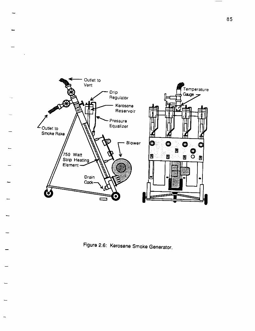
85
tOutlet to
Smoke Rake
Outlet toVent
DripRegulator
KeroseneReservoir
PressureEqualizer
)erature
i! ,,
Figure 2.6: Kerosene Smoke Generator.

- 86
Internal
Filter Bag
SmokeTubes
Heat ExchangerPipes
VerticalDrive
Hose fromSmoke
SmokeFlow
O
,.,=
"=.i
=1
°==
1smokeFlow
.i2
2
I2
[]
.s
22
I
:2
.,!
2
2
22
Figure 2.7: Smoke Rake.

- 87
iiiiiiiii!iii!
£1.
(1)
o
c_c--c_
°_Q.E
E
IJ_
,4oE
(1)(1)o(1)v
IJ..

88
Compressed
Nitrogen Gas
10 psi
v
Needle Valve
To model
v
TiCI4 vapor and Nitogen Gas
-,-,,.o,.,so,.,,,,,Ca,,)iiiiil_iiii',_,[
r"nm'"'rF"'7_itanium Tetrachloride (TiCI_
Figure 2.9: Titanium Tetrachloride Injection System.

89
(End View)
IO00W Flood Lamp
I[ Test Section[[4 8 ft (2.44m)
11
IL_-J,--=-.-J_ 16 mm MotionPicture Camera
(Side View)
Flow Direction
IO00W Flood Lamp
Test Section
Camera
Figure 2.10: 16mm Motion Picture Camera Setup.

co
A
°_
"0
UJV
©
Em
U
EE
u_
©
_';: I:
._ _ : II_" II
d.
E
n-.._1
EE
• .
U-

91
EA
Q,.
Q

ORIGINAL PAGE
BLACK AND WHITE PHOTOGRAPH92
Figure 3.1" Example of a Photographic lmage obtained from aSideView
C O:: ::
E
A
D
Figure 3.2: Schematic of a Photographic lmage obtained from aSideView.
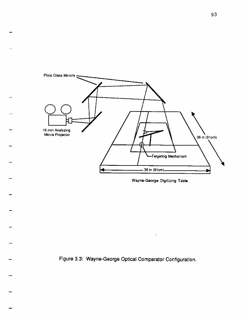
_ 93
Plate Glass Mirrors
©©I
16 mm AnalyzingMovie Projector
36 in (91cm)
_jeting Mechanism
36 in (91cm),
Wayne-George Digitizing Table
Figure 3.3: Wayne-George Optical Comparator Configuration.

- 94ORIGINAE PAGE
BLACK AND WHITE PHOTOGRAPH
Figure 3.4 Example of Photographic Image obtained from a Top View.
C
Figure 3.5: Schematic of Photographic Image obtained from a Top View.

_ 95
(3
O3
0
0
°_
q_
c-
_J
cO
-___.(0
o_
<0
0
.m
--090_._n c0
>_
cO
Q-O(D :_._rrn
-I
U_
_loellV to elOUV

96
o
_loE_,_,Vto el6UV

97
LVDT
LVDTSupport Struct__
Leads to _.
Signal Conditioner'_
® O
Attachment to
Intermediate Linkage
0
m
Support Structure
Figure 4.1" Attachment of LVDT to Delta Wing Pitching Mechanism.

98
1.5
1.0 °
_, 0.5
E
• o.o
-0.5
-I .0
-1.5
29• • I " " I " " I " " I " " | " " I " " I " " I " "
30 31 32 33 34 35 36 37 38
Angle of Attack
Figure 4.2: LVDT Calibration Curve, 29 ° to 38 °.

i
99
90"- (D_>(,3" E
•"=-- r.,O
eLL
a)
2.5 ,
2.0
1.5
1.0 .'-...
0.5 "•
0.0
-0.5
-I.0
-Io5
-2.0
-2o5
0.0
--------- % difference
.......... displacment
0.5 1.0 1.5 2.0Period
Figure 4.3a: One Data Record of the Freesteam Response due to Model Motionfor a Representative Case.
% difference
.......... displacment
0.5 1.0 1.5 2.0period
Figure 4.3b: Ensemble Average of 100 Data Records of the Freestream
Response due to Model Motion for a Representative Case.

lO0
oo
_oet_V lo elOuV
0
c_
o
o
o

-- 101
"10_=O.E<
Figure 4.5a:
2.ooe-2
1.5oe-2
1.0oe-2
5.ooe-3
0.0_+0
Re = 260,000
Angle of Attack = 29 °
0 4 8 12 16 20 24 28 32
Frequency (Hz)
Discrete Fourier Transform of the Variation in Chordwise
Breakdown Location from Mean Position at an Angle of Attackof 29 °. U -- 30 ft/s, Re = 260,000.
"10
_=O.E,<
2.0_-2
1.50e-2
1.0oe-2
5.0_-3
0.0_+0
Re = 260,000
Angle of Attack = 39 °
4 8 12 16 20 24 28 32
Frequency (Hz)
Figure 4.5b" Discrete Fourier Transform of the Variation in Chordwise
Breakdown Location from Mean Position at an Angle of Attackof 39 °. U = 30 ft/s, Re = 260,000.
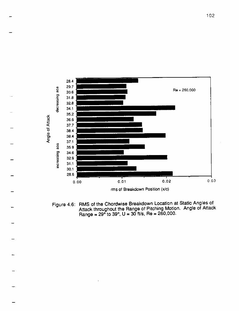
- 102
0
CD_c-
0
<
0
e-"
<00_
C_C
28.4
29.7
30.6
31.8
32.8
34.1
35.2
36.6
37.7
38.4
38.4
37.1
35.9
34.6
32.9
31.1
30.1
28.6
0.00
Re = 260,000
| !
0.01 0.02 0.03
rms of Breakdown Position (x/c)
Figure 4.6: RMS of the Chordwise Breakdown Location at Static Angles of
Attack throughout the Range of Pitching Motion. Angle of AttackRange = 29 ° to 39 °, U = 30 if/s, Re = 260,000.

ORIGINAL PAGE IS
OF POOR QUALITY" 03
4---36o--_
_I----34o_
<1_-- 32 o-.--_
,41.._.-30 o----_
o_Increasing o_ Decreasing(a-e) (f j)
Figure4.7a-j" Sequence of Photographs made from 16ram Movie Film whichIllustrates how the Chordwise Breakdown Location varies
throughout a Pitching Cycle. Angle of Attack Range = 29 =:to 39 _.

104
0
0
!
_0ellV 10 ell_uv
| •
0CO
It'}
0
,5
CO
0
o
e'-._o
,5 8_J
c-
O
• rn
0
°_
0t,-,0
c5
,5
d0
• 0
c_.00 04
(,f)
0
0 _II
O)
_dII
-8,.,
0
II
'sS,_,..._rr'
0 0
_o
e- e-
.__U-
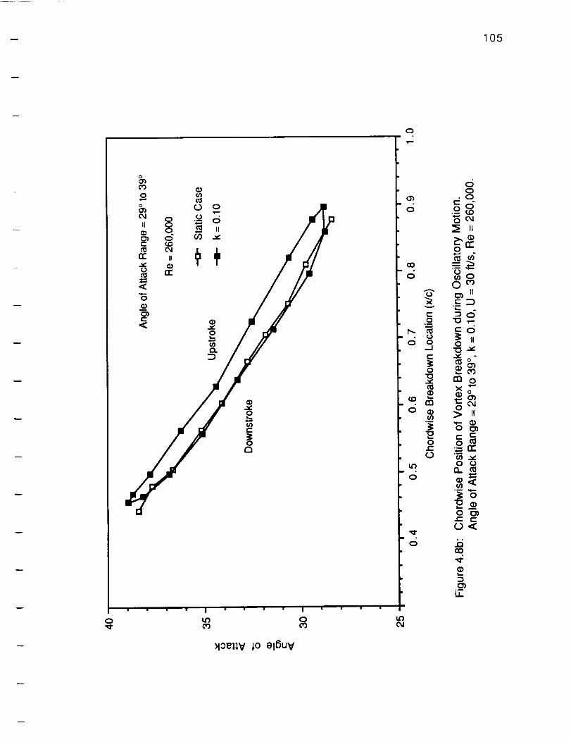
-- 105
o
0,_- CO
Hoel;V ;0 elfiUV
| i
0CO
0
0
0 _"_" II
_- 3(:E
0 0 II
C "_ o"
o _"no
• en "_OC_
g=
° _• _ _
_o
e- e--O<
o .i:i
.__I1

-- 106
0
_0e_le _o ell_UV
0

- 107
0 e3
_0e11V Io el6uV
0
6
t_o4
d0
• 0
_-o"
11
0
o
0II
o_
II
_m
on.0 0
°_ _
_o
e- e--O<
I!

108
00
_lOellV I0 elBuV
o
OO44IP
o 0"-
_d,,,58 _"
-.I o"
rno £
_. =o.o_o,_ _ o
{ g g,-_.._o
o .__ o3"6 o
0 _
o,_n-
6 _
.__LI.

109
oo40
II

II0
Q
o
_lOellV lO elOuV
O3
c;
co
c;
0 'q"-._ -130 ¢'-
0 cO
O'-Cr) II
0 II 03"0 -_ "0
nm O0
OCM
II L'M
_o.=_-_
0
00
o_ "•._ _ (I.)
.__

111
O..00
"1-
0
._o
E
t-,.0z
0.15
0.12
0.09
0.06
0.03
-O-k = 0.05
4, "g" k = 0.10
"_-k = 0.20
k 0.30
Re = 260,000
0,_ ! • ! I ! !
28 30 32 34 36 38 40
Angle of Attack
Figure 4.10a: Width of the Hysteresis Loops, presented in Figures 4.8a-d, overthe Angle of Attack Range of 29 ° to 39 ° for Reduced Frequenciesof k= 0.05,0.10, 0.20, and 0.30. U - 30 ft/s, Re - 260,000.
0.15Q.
8,_1
03"_ 0.12
"1- 0.090
_ o.oe
¢-.2c_ 0.03
c0z
k = 0.20
•-o'- Re = 90,000
Re = 175,000
Re = 260,000
Re = 350,000
0.00 = i w '- ! ' • i28 30 32 34 36 38 40
Angle of Attack
Figure 4.10b: Width of the Hysteresis Loops, presented in Figures 4.9aoc, overthe Angle of Attack Range of 29 ° to 39 ° for Reynolds Number ofRe ---90,000, 175,000,260,000 and 350,000. k = 0.20,U = 10, 20, 30, and 40 ft/s.
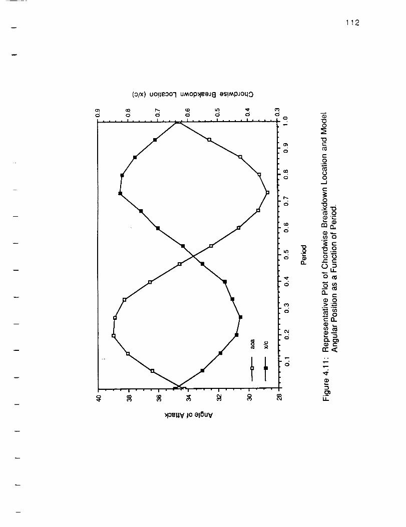
112
0 CO04
13.
0
0
"0r-"
0.q
00
0"0
_ 0O.r-
en_
.m
ge- t-
.,.. U_
0 cn-- a:l
(1) 0
•,-, if)_ 0
m _O--
U.

_ 113
G)
u3
13.
3O
25
20
15
10
5 000o
,,_ Angle of Attack Range =,29 to 39 °O Pl " " • " I .... I .... 1" " • • 1 .... I .... 1 .... I " " "
0.05 0.10 0.15 0.20 0.25 0.30 0.35
Reduced Frequency
0,40
Figure 4.12: Phase Lag of the Vortex Flow as a Function of Reduced Frequencyfor a Reynolds number of 260,000. Angle of Attack Range = 29 °to 39°,U = 30 ft/s.
t,n
"lO
O0
e-13.
3O
25
2O
15
10
(3
• !
0 100000
k = 0.20
Angle of Attack Range = 29 ° to 3g °
• I ° ! '
2ooooo 3ooooo 4ooooo
Reynolds number
Figure 4.13: Phase Lag of the Vortex Flow as a Function of Reynolds Numberfor a Reduced Frequency of 0.20. Angle of Attack Range = 290to 39 ° .
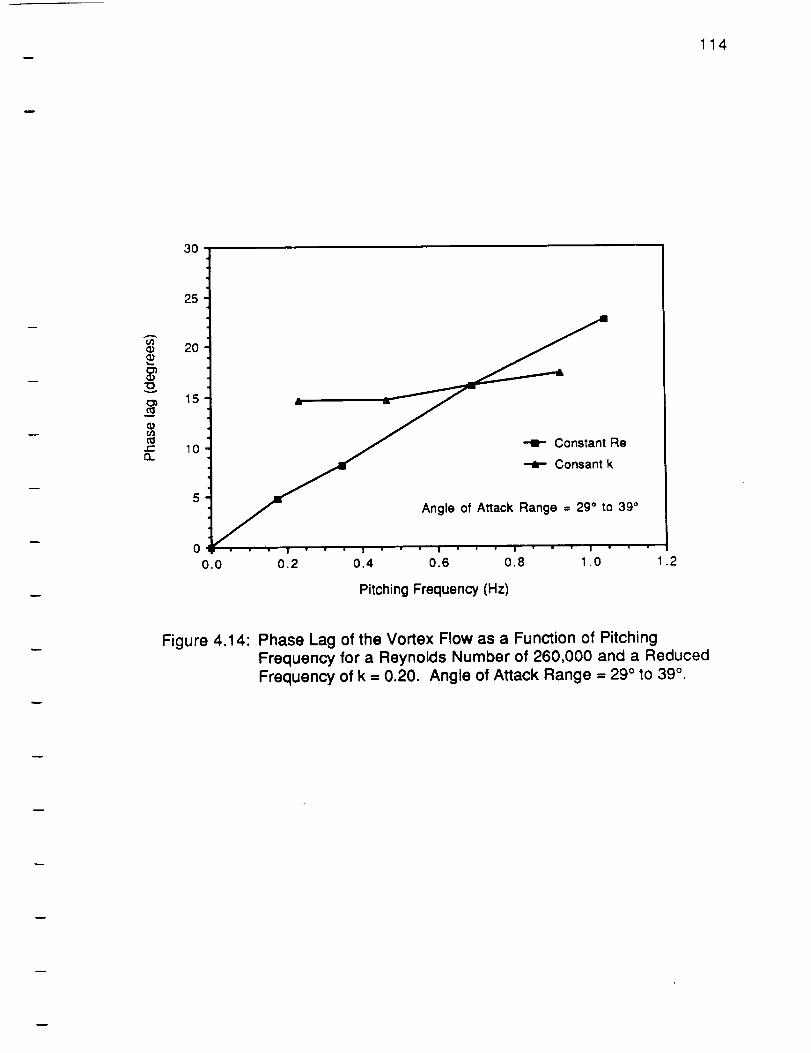
114
'10
o_
13.
30
25
20
15 J.
10 -'] J --as-- Constant Re
Angle of Attack Range = 29° to 39
0 _" I I " " ' I I I
0.0 0.2 1.0 .20.4 0.6 0.8
Pitching Frequency (Hz)
Figure 4.14: Phase Lag of the Vortex Flow as a Function of PitchingFrequency for a Reynolds Number of 260,000 and a Reduced
Frequency of k = 0.20. Angle of Attack Range = 29 ° to 39 °.

115
°oo _2ood oooo
II II II IIOJ
II
0 It) 0 It) 0 it') 0 I._ 0
"T
(s/It} /_!001eA u0!_EOEd0Jd
o
03
o
m.__-,-* rO®_-_
.__> rO 0
¢_ "o0 ,._o
< >o>,d
o_'_coo _o __.o
eh-d"
C3_ d'_
_o.o_o ,i i,
@I,,.

116
ok_
c
0a
0
Q.
• ,, , i ,, ,, i, a w , i ,, , , i w _., i, ; , , i w, ,, i ,,, ,
0 L."I 0 t41 0 tO 0 I._ 0
N ,- ,-- o o o, "7 "7
(s/U) ,_l!OleA u0!le6ed0Jd
o
0
0'_
0
0
OCX, I0') 0. II.=o m
m £zm-_ °._>-8 m
>r'r' .
. OOo> o
o £ h" o_co n
,,
Oc5

117
o
c/)¢-
oa
0o c5 c5 c5
t4_ II II II II
,,s ,.o _ ,.,II
• ' '" I "" '' I'' "" I " _' ' I' ''' I'" ''| " ' "' I ' "" "
(/o/n) ,_l!oOleA peonpeu
o
o_
=-o<.._o o o
>_
_ °e" "_Do o__ _0. _
m-Sd_
_dm
k....
__
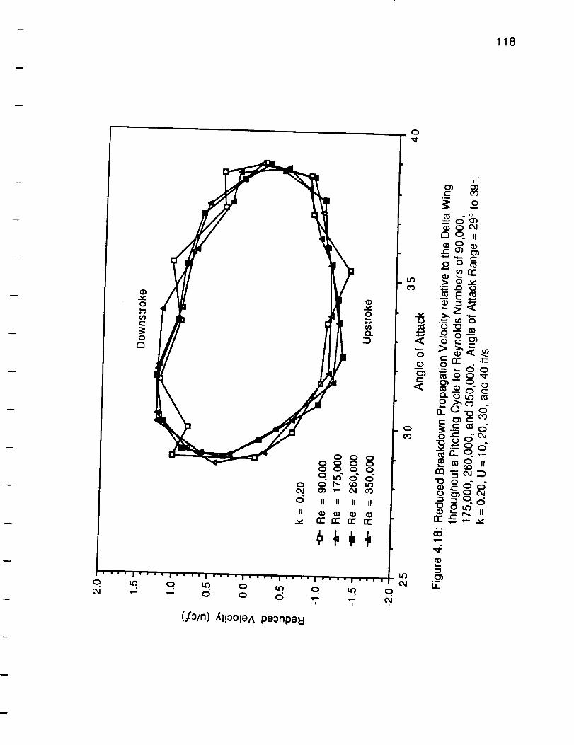
!
118
0
(/o/n) ,O,!ooleA peonpeEI

29.5
30.8o
32.6e-•_ 34.5
_ 36.4
-o 37.9v.o 38.8
< 39.1
o 38.3
37.1t"
< _ 35.40
33.3m= 31.5
_ 30.1
.-_ 29.1
28.9
0.00
Figure 4.19a:
28.8
29.70
31.10')¢--_ 32.9
34.9
-_ 36.8
o 38.2
< 38.9
o 38.9
38.1C
< _ 36.5o
34.8
" 32.8
30.9
._c 29.6
28.7
0.00
Figure 4.19b:
119
r r0.01 O.O2
rms of Breakdown Position (x/c)
20 cycles
k = 0.20
Re = 260,000
0.03
RMS of the Chordwise Breakdown Location at Various Angles of
Attack throughout a Pitching Cycle. Angle of Attack Range = 29 °to 39 °, k = 0.20, U -- 30 if/s, Re - 260,000.
I !
0.01 0.02
rms of Breakdown Location (x/c)
12 cycles
k = 0.20
Re = 175,000
0.03
RMS of the Chordwise Breakdown Location at Various Angles of
Attack throughout a Pitching Cycle. Angle of Attack Range = 29 °to 39 °, k = 0.20, U -- 20 ft/s, Re - 175,000.

ORIGINAL PAGE
BLACK AND WHITE PHOTOGRAPH
Figure 4.20a: Photograph used to Demonstrate that the Vortex Core can beAssumed to be Straight. Angle of Attack = 29 °, U = 30 ft/s.Re = 260,000.
Figure 4.20b' Photograph used to Demonstrate that the Vortex Core can beAssumed to be Straight. Angle of Attack = 39 °, U = 30 ft/s,
Re = 260,000.
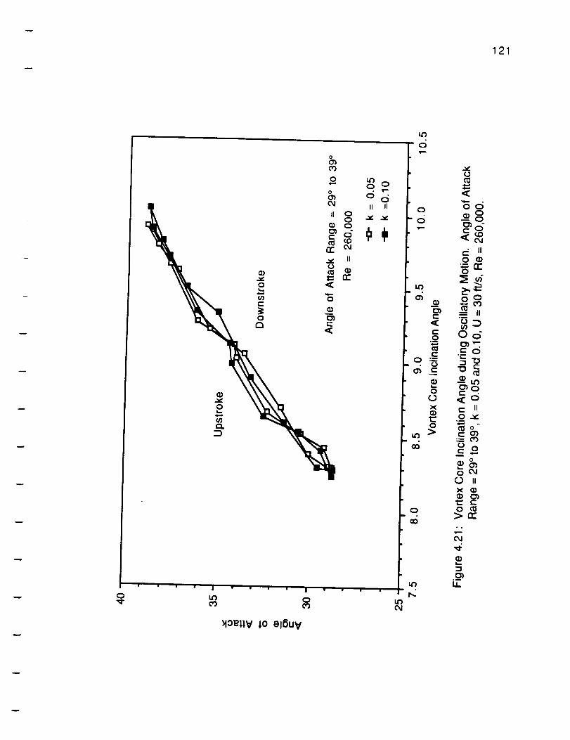
121
0
_10eJ,:lV;0 el6UV
o
,,<,,e=,.
oo_=oo
II0
0
"-" II
oC)t,/)oo"
c(:5
a_
u
°_
•-- 030¢,- 0
OC_C) IIx
0 ¢0
o4
q)
U.

- 122
0| • • • • |
It) 0cO
)10_i_V_0 elSuV
o
a;
e-,<c._o
e-0 "--
0
X
0
0
<
oo0
0 •
0
0 0•.-, o*)
--- II
(/)
O_I_0")
--_0
,<oe- iio-_
_ o¢- .,...,
0
0 II
x _)_P O)1:: c::0>r'r"
o,I
.m
LI.

- 123
0
o
Q..
_toeJ,J,V _o el6UV
003
unCq
_r_
¢1-- 0
<d• _
g ,
°_
O_
•t- II
It
_ 0e- .,..,
0
x
0_>_..
c,,J
-'1
I,,I-

124
| • • • •
:I0_J4¥_0 elOu¥
| • • • •
,5
o0
X
0>
k_
a0
0
ao
14")
d00
-=o"c) 14)
:I::
0 c0
00
_0
<o_04.£ iI
orr
_0
"0 "0
Oe_
"_- II
_6II
0 0
0
_m0 IIx
c
l,J,.

ORIGINAL PAGE
BLACK AND WHITE PHOTOGRAPH!25
.4--- 40 _--.-._
,ql--.- 20 o--_
_1.--- 10_-_ •
c_ Increasing c_ Decreasing(a-e) (f-j)
Figure 4.25a-j: Sequence of Photographs made from 16mm Movie Film whichIllustrates how the Chordwise Breakdown Location varies
throughout a Pitching Cycle. Angle of Attack Range = 0: to _5 _,k = 0.30, U = 30 ft/s, Re = 260,000.
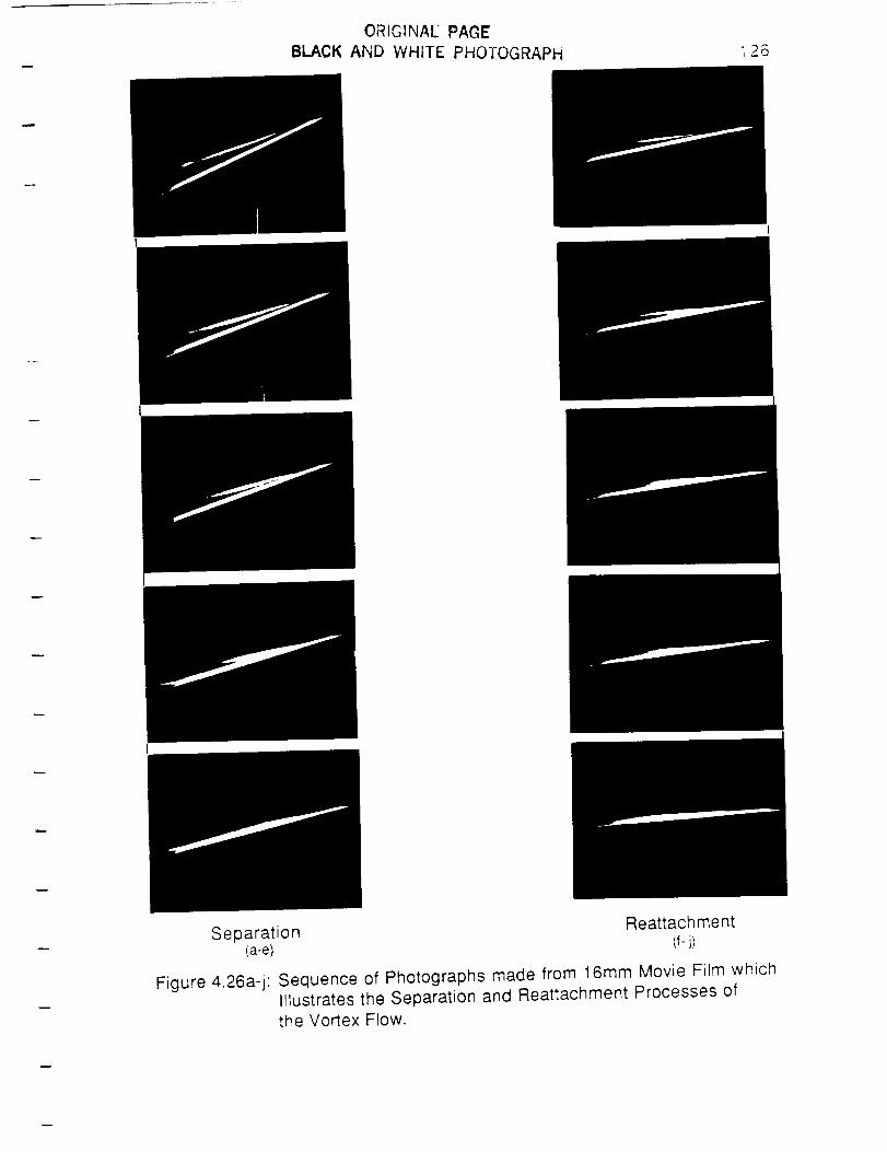
ORIGINALPAGEBLACK AND WHITE PHOTOGRAPH 126
I
Separation Reattachment(a-e) d-J)
Figure 4.26a-j Sequence of Photographs made from 16mm Movie Film whichIllustrates the Separation and Reattachment Processes of
the Vortex Flow.

127
00 _ 00 0 03
(,0 II II('_
II
"'''l''''i''''l''''l'''"
0 0 _ O Q
M0e;),V ;o el6uV
0
0
00
Q
A(,3"R
t-O
f,O
(,30
_J
0
(2)
t'n
0t-
O
04
0
0
0
(.-:0
0-,-' II
©m
•_,- _:_
_d0
"agCO "_"
x 0
0
0 _
'_
o-_d(1_ _0
_
o ,,:( rr
Od
.__L.L.

- 128
o 0,,,¢
0¢0
_10e_V
0
j0 elOuV
0 0

- 129
0
o
0
T,=-
e-<t-._o
e-
x
(o o
o• • • • | I • • • | • • • • | • = • • | • • = •
0 0 _ Q 0
_10eP,V 10 ell_uv
o
¢.-<8c-O II
0
II
0
"_ 0
..0.- o
¢" 0<ot-O II
_- o
0
X _
a:i
U-

130
(OIX) uo!leoo-I u_AoP_leeJIBes!MpJoqo
,,- ,- (5 ,:5 ,:5 o o ,::5 o.... I _, , , I j , ,. I .... I.... I.... I.... I .... 0
o u") 0 i._¢0 o'J 0,1
)loeJ,),VIo el6uV
>
03(3.E om 0
(Ifc"_l
0 II
(P O}•m t-"0
u") _rr
.0
fo
0 :I=
Wl--
°oo
•i
c> m_rr
" o _o
_J "6< "
o ,_-_
.__
0

131
_loel_,V ;o el_uV

- 132
[]
o
II
Lr) 0 0o _. _.o o otl II II
E!
[]
m[]
• II
i'll
!
I.¢')I
o¢,,.)
• II
&
o&(M
0 II
8 ®t2)
t,D
II
er
o
C
o
6
o
o
o
ti.
ei
Q.
d0
0
'*" O
="t3•_ (.'-
Oo04
fd
_0
0.._
•_ O"
_C_
I:I_oxo_C_
0 I1__0
'.= II
0 tUn"n_
C_llQ.c--
Cr')
I.I.
_loellV,_oelOuV

APPENDIX A
Discrete Fourier Transforms of Model Motion
133

o "_.
epnl!lduJV
o
8o.
o
"i-v
O"
I.L.
o
o
o
0
O3
0
0
U
rr
r_
134
0
¢-
_o
"0
O0
IIa_
• •
._m1..1..

o • o
epnl!IduJV
o
J
_=iii
J
q
,-I
d
d
oo4
N
•._ ul
q
J
u
oo
A
N"I-
(D
0
0 =
LL
0
O_
0
0
II
C
n"
<0
<
o_o_
o_
II
&i<
°_
U.
135

136
"-:.
epnl!IdLuv
o
o
kcJ
o
..#"t-
,z.=
0"
I.I_
0
CO
0
0
0'_
II
(DO_¢-n_
.=_0
0
(D
0
0
"00
0
u.121
/6
u_
0
II
dII
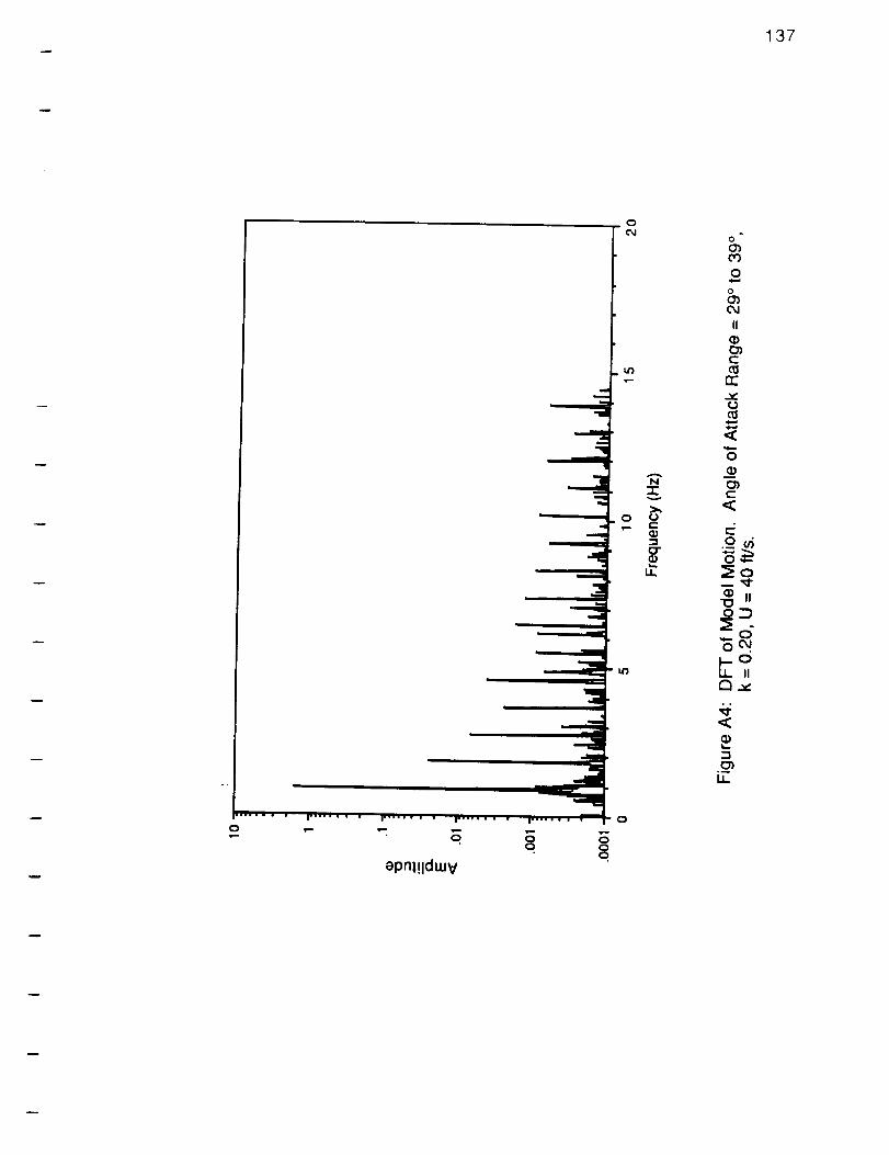
137
o
m
-,j
i |
| i
i
..q
fo.w • • • •
!
|...= • • • • r.=_ • • • •
epnl!Idwv
"'111
,-.,,,,=
.-L
allI I I,
,.,.,11
I....... |
00
q
ockl
o
Lt_
0
A
N"I-v
(.)
-iO"
ii
0
O3eg
0
0
(3"}¢M
II
(P0")E:
rr
(J
0
<
.g _,i
_o
"10o_
0
IIa_
<
U.

138
oii,,,,, • • •
'r--
,j
|,.,,= • • • i,,.,0 • • •
-. 3 oo
epni!IduJV
3Qo.
o
c_
o
o4
N"I"
u,') U• c
',,-
0"
o
o
o
0
0
0
0
II
e-
U
<
0
<
o_o_
o_
o_l_u. /0 o
II
,<
U.

o • o
epn|!IduJV
3
i
--T==.._1
oo_
o.
N"1-
rJC
0"
LI=
0
L_
0
0
II
0")
n"v'0
.4==*
<
0
01
139
t-,,<
o_o__o
(I) II"0o_
OCO
II
13,,,
,<
°_
t.L

APPENDIX B
Freestream Velocity Fluctuation and Model Position
140

141
>,,4-)4,4
00
@
C3E<O@ @L >
.,-4
@ 0
L @U_n"
i
i
//
\\
\
//
uy
//
\
X_oO[eA woaJ_s_eJ_ uo_ woJ_
ocO
<
0
q_
<
0
0O.
"0o_
"00_e3
IIE
"10_d
U. ,.,,
0
0>_
u n-• °
m
u.

142
>,.
• r-',l
(J0
@> <
OE <0@ @L >4.) .,-4@ 40@ O
L @h. rv
i
I
\
/
130.t-I
L@O_
|°..,ll *_
i •
I I I
(o
O
c-
Oo_
coO13.
"13o_
"130t'- _.._
IIt-O=)
Nu4
_6
ii .._
_ 0
o__ 0:'2"E_
e-
&ien
L-
U.

143
>,,
4,'4
00
@
QE <0@ @L >43 ,,-4
@ 0
L @
I' I
U'l 0i i
X_Too[eA
\\
>/
Ill 0 c_ U'l 0 Lr)i i
I I [
womJ%ssmJj uom_ woJ_ _0 %
.m-*
0
O)
O)E<(
0°_
(/)0O.
"I0
"00c--_
o: II
o_
.$..,oO
:3 IIU._
4-_ 0
>r'E _
_ E
b.i
0_
U.
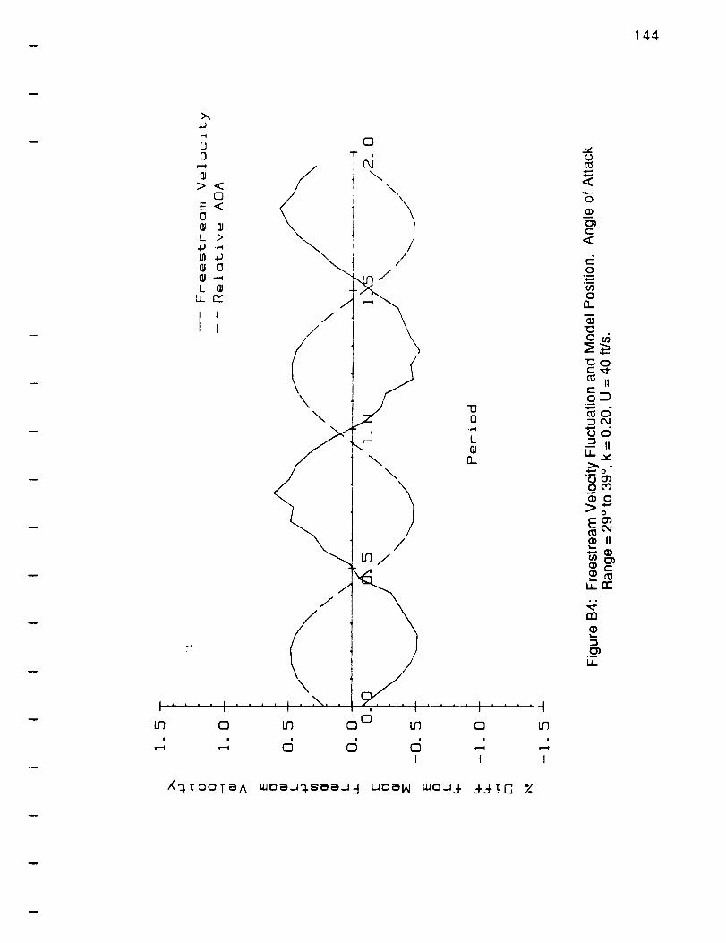
144
II
U3o
0
,$,-
0
O1t-
O°_
013.
nOO_
"130
oC)
oc5---_ IIU._,g
>;--E _
rn
°_
LI_

145
\
//
\
L_ 0 _ 0 _ 0 {2) U'l C_ _ 0
i i i i
I I I I
LA
I
(DCO
<
0
r-<
0
00_
(1)
0
r.- o_c_
c II0
_di1 II
>o
_ben
.__

146
X_;oOIeA
0 Lr) 0 0 U'l 0 U'l 0 l.r)
.4 d d 5 ,4 ,4 N NI I I I I
wDaJ%se_JJ uoeH
(J
<
0
r-<
0°_
0_00.
7O0
"*"cO0
U. II
OoOt_'3
>o
c
.__U-

APPENDIX C
Chordwise Breakdown Location and Model Position
147

148
(o/x) uoT_moo 7 uMopNmeu8 es[MpJoq3
C3
I
m
d
730
L@
a_
Oo_0_qe-O
d II
0.._
.oe,_o ii_D
_u4(-
e-OO II
0Oo
e-_oOo
,,¢_j
m_
O _e":l _0'<
• •
0

149
-4 6 6 d
(o/x) uo_ooo7 w_opHo_JB es_mPJOq3

- 150
_ c_ d d d d d
0
L
(I.
t-O
o_
0 0>_rr03o_
-OO30 II
_cxl
,--d0 II
Oo
c-
Oo
m_
•_ n,-
b_
.__
(_/X) uOT_O00_ uMOpHO_ 8 _STMp_Oq3
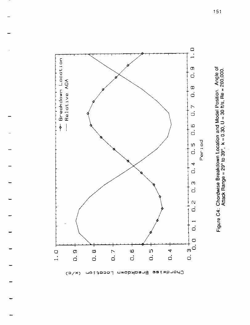
151
0 _ O0 h, _ LO "_
,-; d d d d c_ d
(3/x) uMopHoeuB eS_MpJOqD
oo
_0
d ii0"_rro--
o_
-0 c_'}0 IINDnOcd
0 II
Qo
Oo
_ c.-
0

152
(3
• ! ' ' I .... I ! " ' _ I .... I
E0
.T-'I
430(J0 '_
I 0
cOJ
O >-0 .,-.4
0 0
L03 n-
• . , ! .... ! ....
L-| | ' I ....
01 03 [',. K3 LR
d d d d d d
(o/x) uo_eooq uMopHoeJ 8 esTMpJoq 3
0
O0
0
b-
0
(3
0
0
m
0
(_
0
0
0
m o
d
0
L
13...
0_6
,,(I_0
odm_NoO I|
_D,--dt_¢xl
O II
OOo
t-_oOo"Ot:_.-_C4
_ Hen_
•_ n"
O
t_

153
0i
(_/x) uo_moo 7 uMopHoaJ B as_Mp_oq3
0
0
O3
0
b--
0
lO
0
LO
0
0
m
o
f_
o
o
0
m o
d
0
L0O_
oo
,
_rro0
nocxlo ii
_D
c_0_cxJ
o II_,,,e
oo
c::_oOo"_o_
lio)
e.-:_
II

154
0 _ O3 ["- £0 Lrl
,-; 5 d d d 5 d
(3/x) uoT_oooq uMopHom_8 as_MP_°q3
O3
0
0
0
o(5Q) O
(-0
C4
0.=_rr
n
_o
0 IIND
co0 II
0 0•.4 0 o
Oo
0 _e.-:_
"1
o--

155
.... I .... ! .... I " " "
C0
,r-I
0(J0_J 0
<C
00 >
7_ '"_
0 00L @
rnn,
CO
0
N
d
d
(o/x) uo_moo7 uMopHoe_8 _s_Mp_o43
"D0.r'l
L@(I.
Oo
0
{/)od
o It
r-
e-O0 II
0 .Oo
c-
Oo
i1_ II
o_
0

156
(O/X) uO_%00o 7 uMOp_O@_ B as_MpJo4o
O0
0
0
L@O_
0
mo
_0
c- II0
"_ 13:
-00
0c d0
0_1o
@ II
en_
•_ n"
0
0
U.

157
..... I .... I ........ 1 .... I .... I .... I .... ! .... I ....
/(:3.<
C
0 >.,..4,,.J
0 00,-4L _1
rnn,"
+1
C3 (3) 03 P'- LO Lr] 4- f'O ('&l
,-; 5 5 5 5 5 5 5 5 5
(o/x) uoT#Doo 7 uMopNoe_ 8 esTap_o4 3
C3

REFERENCES
Bragg, M. and Soltani, M., "Experimental Measurements on an Oscillating 70 °Delta Wing in Subsonic Flow," Report presented at NASA LanleyResearch Center, VA, December 10, 1987.
Corporon, P. G., "Wayne-George Optical Comparator-to-DEC DRV-11 ParallelLine Unit Interface Board User's Manual, University of Notre Dame,"June, 1987.
Cunningham, A. M., "Vortex Flow Hysteresis," NASA-CP-2416, No. 11, October1985.
Elle, B. J., "An Investigation at Low Speed of the Flow Near the Apex of ThinDelta Wings with Sharp Leading Edges," Aeronautical Research Council,R & M No. 3176, 1958.
Erickson, G. E., "Vortex Flow Correlation," Tech Rept. AFWAL-TR-80-3143,January,1981.
Gad-eI-Hak, M. and Blackwelder, R. F., "The Discrete Vortices from a Delta
Wing," AIAA Journal, Volume 23, No. 6, June 1985, p 961.
Gad-eI-Hak, M., Ho, C. M., and Blackwelder, R. F., "A Visual Study of a DeltaWing in Steady and Unsteady Motion," Proceedings of the Workshop onUnsteady Separated Flows, editors M. S. Francis and M. W. Luttges,Colorado Springs, Colorado, August 1983.
Gad-eI-Hak, M. and Ho. C. M., "The Pitching Delta Wing," AIAA Journal, Volume23, No.11, 1985, pp1660-1665.
Gilliam, F., Robinson, M., Walker, J. and Wissler, J., "Visualization of UnsteadySeparated FI.ow About a Pitching Delta Wing," AIAA 25th AerospaceSciences Meeting, Jan 12-15, 1987, Reno Nevada.
Herbst, W. B., "Supermaneuverability," Proceedings of the AFOSR-FJSRL-University of Colorado Workshop on Unsteady Separated Flow, USAFAcademy, CO, August 1983.
Lambourne, N. C., Bryer, D.W. and Maybrey, J. F. M. "The Behavior of LeadingEdge Vortices over a Delta Wing Following a Sudden Change inIncidence," Aeronautical Research Council, R & M No. 3645, 1969.
158

159
Lambourne, N. C. and Bryer, D. W., "The Bursting of Leading Edge Vortices--Some Observations and Discussion of the Phenomena," Aeronautical
Research Council, R & M No. 3282, April 1961.
Lee, M., Shih, C. and Ho, C. M., "Response of a Delta Wing In Steady andUnsteady Flow," 1987 ASME Applied Mechanics, Bioengineering andFluid Engineering Conference, Cincinnati, Ohio, June 14-17, 1987.
Lowson, M. V., "Some Experiments with Vortex Breakdown," Journal of theRoyal Aeronautical Society, Vol 68, pp. 343-346, 1964.
Malcolm, G. N., "Impact of High-Alpha Aerodynamics on Dynamic StabilityParameters of Aircraft and Missies," AGARD LS No. 114, March 1981.
Malty, R. L., Enger, P. B. and Keating, R. F. A., with Addendum by Moss, G. F.,"Some Exploratory Measurements of Leading-Edge Vortex Positions ona Delta Wing Oscillating in Heave," Aeronautical Research Council, R &M No. 3176, July 1963.
Reynolds, G. A. and Abtahi, A. A., "Instabilities in Leading-Edge VortexDevelopment," AIAA-87-2424, Applied Aerodynamics and AtmosphericFlight Mechanics Conference, August 17 - 19, 1987.
Rockwell, D., Atta, R., Kuo, C. -H., Hefele, C., Magness, C. and Utsch, T., "OnUnsteady Flow Structure from Sweep Eddies Subjected to Controlled
Motion," Paper presented at AFOSR Workshop on Unsteady SeparatedFlows, USAF Academy, CO, July 26 - 30, 1987.