lncs 4232 - learning hierarchical bayesian networks for...

Learning Hierarchical Bayesian Networksfor Large-Scale Data Analysis

Kyu-Baek Hwang1, Byoung-Hee Kim2, and Byoung-Tak Zhang2

1 School of Computing, Soongsil University,Seoul 156-743, [email protected]

2 School of Computer Science and EngineeringSeoul National University,

Seoul 151-742, [email protected],

[email protected]

Abstract. Bayesian network learning is a useful tool for exploratorydata analysis. However, applying Bayesian networks to the analysis oflarge-scale data, consisting of thousands of attributes, is not straight-forward because of the heavy computational burden in learning and vi-sualization. In this paper, we propose a novel method for large-scaledata analysis based on hierarchical compression of information and con-strained structural learning, i.e., hierarchical Bayesian networks (HBNs).The HBN can compactly visualize global probabilistic structure througha small number of hidden variables, approximately representing a largenumber of observed variables. An efficient learning algorithm for HBNs,which incrementally maximizes the lower bound of the likelihood func-tion, is also suggested. The effectiveness of our method is demonstratedby the experiments on synthetic large-scale Bayesian networks and areal-life microarray dataset.

1 Introduction

Due to their ability to caricature conditional independencies among variables,Bayesian networks have been applied to various data mining tasks [9], [4]. How-ever, application of the Bayesian network to extremely large domains (e.g., adatabase consisting of thousands of attributes) still remains a challenging task.General approach to structural learning of Bayesian networks, i.e., greedy search,encounters the following problems when the number of variables is greater thanseveral thousands. First, the amount of running time for the structural learningis formidable. Moreover, greedy search is likely to be trapped in local optima,because of the increased search space.

Until now, several researchers suggested the methods for alleviating the aboveproblems [5], [8], [6]. Even though these approaches have been shown to effi-ciently find a reasonable solution, they have the following two drawbacks. First,they are likely to spend lots of time to learn local structure, which might be

I. King et al. (Eds.): ICONIP 2006, Part I, LNCS 4232, pp. 670–679, 2006.c© Springer-Verlag Berlin Heidelberg 2006

Learning Hierarchical Bayesian Networks for Large-Scale Data Analysis 671

less important in the viewpoint of grasping global structure. The second prob-lem is about visualization. It would be extremely hard to extract useful knowl-edge from a complex network structure consisting of thousands of vertices andedges.

In this paper, we propose a new method for large-scale data analysis usinghierarchical Bayesian networks. It should be noted that introducing hierarchicalstructures in modeling is a generic technique. Several researchers have intro-duced the hierarchy to probabilistic graphical modeling [10], [7]. Our approachis different from theirs in the purpose of hierarchical modeling. The purposeof our method is to make it feasible to apply probabilistic graphical modelingto extremely large domain. We also propose an efficient learning algorithm forhierarchical Bayesian networks having lots of hidden variables.

The paper is organized as follows. In Section 2, we define the hierarchicalBayesian network (HBN) and describe its property. The learning algorithm forHBNs is described in Section 3. In Section 4, we demonstrate the effectivenessof our method through the experiments on various large-scale datasets. Finally,we draw the conclusion in Section 5.

2 Definition of the Hierarchical Bayesian Network forLarge-Scale Data Analysis

Assume that our problem domain is described by n discrete variables, Y ={Y1, Y2, ..., Yn}.1 The hierarchical Bayesian network for this domain is a spe-cial Bayesian network, consisting of Y and additional hidden variables. It as-sumes a layered hierarchical structure as follows. The bottom layer (observedlayer) consists of the observed variables Y. The first hidden layer consists of�n/2� hidden variables, Z1 = {Z11, Z12, ..., Z1�n/2�}. The second hidden layerconsists of �(�n/2�)/2� hidden variables, Z2 = {Z21, Z22, ..., Z2�(�n/2�)/2�}. Fi-nally, the top layer (the �log2 n�-th hidden layer) consists of only one hid-den variable, Z�log2 n� = {Z�log2 n�1}. We indicate all the hidden variables asZ = {Z1,Z2, ...,Z�log2 n�}.2 Hierarchical Bayesian networks, consisting of thevariables {Y,Z}, have the following structural constraints.

1. Any parents of a variable should be in the same or immediate upper layer.2. At most, one parent from the immediate upper layer is allowed for each

variable.

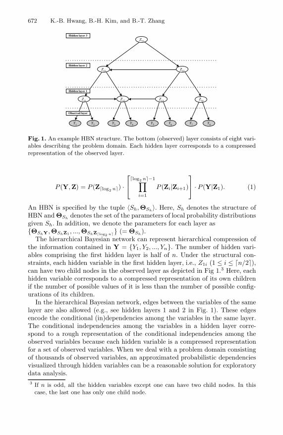
Fig. 1 shows an example HBN consisting of eight observed and seven hiddenvariables. By the above structural constraints, a hierarchical Bayesian networkrepresents the joint probability distribution over {Y,Z} as follows.

1 In this paper, we represent a random variable as a capital letter (e.g., X, Y , andZ) and a set of variables as a boldface capital letter (e.g., X, Y, and Z). Thecorresponding lowercase letters denote the instantiation of the variable (e.g., x, y,and z) or all the members of the set of variables (e.g., x, y, and z), respectively.

2 We assume that all hidden variables are also discrete.

672 K.-B. Hwang, B.-H. Kim, and B.-T. Zhang

Z11

Observed layer

Hidden layer 2

Hidden layer 3

Hidden layer 1

Y2 Y8Y7Y6Y5Y4Y3Y1

Z12 Z13 Z14

Z21 Z22

Z31

Fig. 1. An example HBN structure. The bottom (observed) layer consists of eight vari-ables describing the problem domain. Each hidden layer corresponds to a compressedrepresentation of the observed layer.

P (Y,Z) = P (Z�log2 n�) ·

⎡⎣�log2 n�−1∏

i=1

P (Zi|Zi+1)

⎤⎦ · P (Y|Z1). (1)

An HBN is specified by the tuple 〈Sh,ΘSh〉. Here, Sh denotes the structure of

HBN and ΘShdenotes the set of the parameters of local probability distributions

given Sh. In addition, we denote the parameters for each layer as{ΘShY,ΘShZ1 , ...,ΘShZ�log2 n�} (= ΘSh

).The hierarchical Bayesian network can represent hierarchical compression of

the information contained in Y = {Y1, Y2, ..., Yn}. The number of hidden vari-ables comprising the first hidden layer is half of n. Under the structural con-straints, each hidden variable in the first hidden layer, i.e., Z1i (1 ≤ i ≤ �n/2�),can have two child nodes in the observed layer as depicted in Fig 1.3 Here, eachhidden variable corresponds to a compressed representation of its own childrenif the number of possible values of it is less than the number of possible config-urations of its children.

In the hierarchical Bayesian network, edges between the variables of the samelayer are also allowed (e.g., see hidden layers 1 and 2 in Fig. 1). These edgesencode the conditional (in)dependencies among the variables in the same layer.The conditional independencies among the variables in a hidden layer corre-spond to a rough representation of the conditional independencies among theobserved variables because each hidden variable is a compressed representationfor a set of observed variables. When we deal with a problem domain consistingof thousands of observed variables, an approximated probabilistic dependenciesvisualized through hidden variables can be a reasonable solution for exploratorydata analysis.3 If n is odd, all the hidden variables except one can have two child nodes. In this

case, the last one has only one child node.


3 Learning the Hierarchical Bayesian Network

Assume that we have a training dataset for Y consisting of M examples, i.e.,DY = {y1,y2, ...,yM}. We could describe our learning objective (log likelihood)as follows.

L(ΘSh, Sh) =

M∑m=1

log P (ym|ΘSh, Sh) =

M∑m=1

log∑Z

P (Z,ym|ΘSh, Sh), (2)

where∑

Z means summation over all possible configurations of Z. General ap-proach to finding maximum likelihood solution with missing variables, i.e., theexpectation-maximization (EM) algorithm, is not applicable here because thenumber of missing variables amounts to several thousands. The large number ofmissing variables would render the solution space infeasible.

Here, we propose an efficient algorithm for maximizing the lower bound ofEqn. (2). The lower bound for the likelihood function is derived by Jensen’sinequality as follows.

M∑m=1

log∑Z

P (Z,ym|ΘSh, Sh) ≥

M∑m=1

∑Z

log P (Z,ym|ΘSh, Sh). (3)

Further, the term for each example, ym, in the above equation can be decom-posed as follows.∑Z

log P (Z,ym|ΘSh, Sh) =

∑Z

log P (ym|ΘShY, Sh) · P (Z|ym,ΘSh\ΘShY, Sh)

= C0 · log P (ym|ΘShY, Sh) +∑Z

log P (Z|ym,ΘSh\ΘShY, Sh), (4)

where C0 is a constant which is not related to the choice of ΘShand Sh. In

Eqn. (4), the parameter sets ΘShY and ΘSh\ΘShY can be learned separately

given Sh.4 Our algorithm starts by learning ΘShY and the substructure of Sh

related to only the parents of Y. After that, we fill missing values for the variablesin the first hidden layer, making the training dataset for Z1.5 Now, Eqn. (4) canbe more decomposed as follows.

C0 · log P (ym|ΘShY, Sh) +∑Z

log P (Z|ym,ΘSh\ΘShY, Sh)

= C0 · log P (ym|ΘShY, Sh) + C1 · log P (z1m|ΘShZ1 , Sh)

+∑Z\Z1

log P (Z\Z1|ym, z1m,ΘSh\{ΘShY,ΘShZ1}, Sh), (5)

4 In this paper, the symbol ‘\’ denotes set difference.5 Because hidden variables are all missing, this procedure is likely to produce hidden

constants by maximizing the likelihood function. We apply an encoding scheme forpreventing this problem, which will be described later.


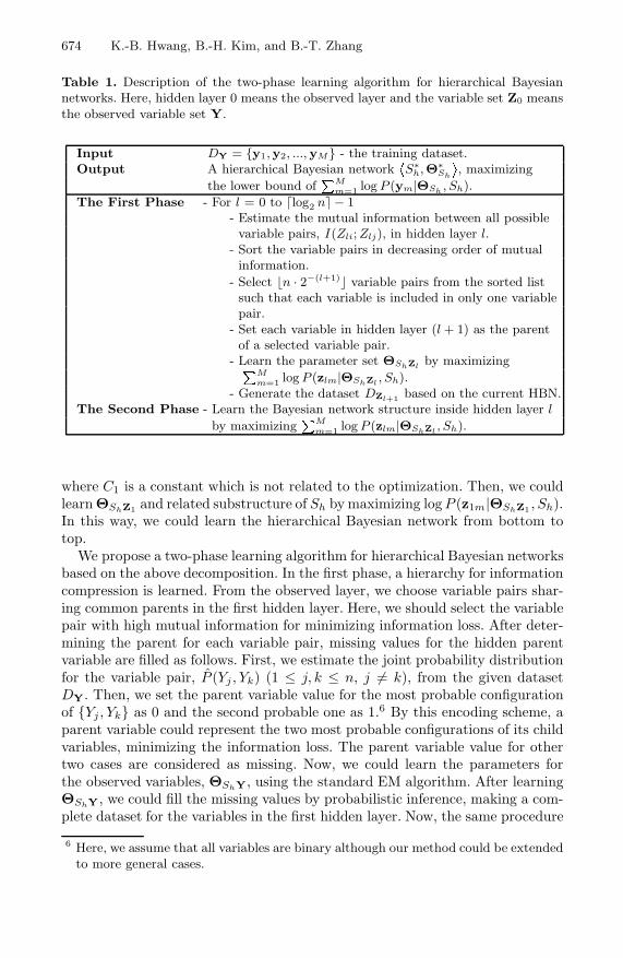
Table 1. Description of the two-phase learning algorithm for hierarchical Bayesiannetworks. Here, hidden layer 0 means the observed layer and the variable set Z0 meansthe observed variable set Y.

Input DY = {y1,y2, ..., yM} - the training dataset.Output A hierarchical Bayesian network

�S∗

h,Θ∗Sh

�, maximizing

the lower bound of�M

m=1 log P (ym|ΘSh , Sh).The First Phase - For l = 0 to �log2 n� − 1

- Estimate the mutual information between all possiblevariable pairs, I(Zli; Zlj), in hidden layer l.

- Sort the variable pairs in decreasing order of mutualinformation.

- Select �n · 2−(l+1)� variable pairs from the sorted listsuch that each variable is included in only one variablepair.

- Set each variable in hidden layer (l + 1) as the parentof a selected variable pair.

- Learn the parameter set ΘShZl by maximizing�Mm=1 log P (zlm|ΘShZl , Sh).

- Generate the dataset DZl+1 based on the current HBN.The Second Phase - Learn the Bayesian network structure inside hidden layer l

by maximizing�M

m=1 log P (zlm|ΘShZl , Sh).

where C1 is a constant which is not related to the optimization. Then, we couldlearn ΘShZ1 and related substructure of Sh by maximizing log P (z1m|ΘShZ1 , Sh).In this way, we could learn the hierarchical Bayesian network from bottom totop.

We propose a two-phase learning algorithm for hierarchical Bayesian networksbased on the above decomposition. In the first phase, a hierarchy for informationcompression is learned. From the observed layer, we choose variable pairs shar-ing common parents in the first hidden layer. Here, we should select the variablepair with high mutual information for minimizing information loss. After deter-mining the parent for each variable pair, missing values for the hidden parentvariable are filled as follows. First, we estimate the joint probability distributionfor the variable pair, P (Yj , Yk) (1 ≤ j, k ≤ n, j �= k), from the given datasetDY. Then, we set the parent variable value for the most probable configurationof {Yj , Yk} as 0 and the second probable one as 1.6 By this encoding scheme, aparent variable could represent the two most probable configurations of its childvariables, minimizing the information loss. The parent variable value for othertwo cases are considered as missing. Now, we could learn the parameters forthe observed variables, ΘShY, using the standard EM algorithm. After learningΘShY, we could fill the missing values by probabilistic inference, making a com-plete dataset for the variables in the first hidden layer. Now, the same procedure

6 Here, we assume that all variables are binary although our method could be extendedto more general cases.


can be applied for Z1, learning the parameter set ΘShZ1 and generating a com-plete dataset for Z2. This process is iterated, building the hierarchical structureand making the complete dataset for all variables, {Y,Z}.

After building the hierarchy, we learn the edges inside a layer when necessary(the second phase). Any structural learning algorithm for Bayesian network canbe employed because a complete dataset is now given for the variables in eachlayer. Table 1 summarizes the two-phase algorithm for learning HBNs.

4 Experimental Evaluation

4.1 Results on Synthetic Datasets

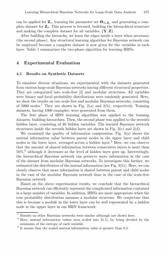
To simulate diverse situations, we experimented with the datasets generatedfrom various large-scale Bayesian networks having different structural properties.They are categorized into scale-free [2] and modular structures. All variableswere binary and local probability distributions were randomly generated. Here,we show the results on two scale-free and modular Bayesian networks, consistingof 5000 nodes.7 They are shown in Fig. 2(a) and 2(b), respectively. Trainingdatasets, having 1000 examples, were generated from them.

The first phase of HBN learning algorithm was applied to the trainingdatasets, building hierarchies. Then, the second phase was applied to the seventhhidden layer, consisting of 40 hidden variables. The learned Bayesian networkstructures inside the seventh hidden layer are shown in Fig. 2(c) and 2(d).

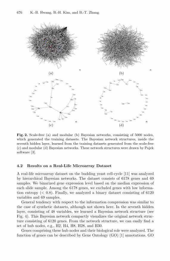
We examined the quality of information compression. Fig. 3(a) shows themutual information value between parent nodes in the upper layer and childnodes in the lower layer, averaged across a hidden layer.8 Here, we can observethat the amount of shared information between consecutive layers is more than50%,9 although it decreases as the level of hidden layer goes up. Interestingly,the hierarchical Bayesian network can preserve more information in the caseof the dataset from modular Bayesian networks. To investigate this further, weestimated the distribution of the mutual information (see Fig. 3(b)). Here, we canclearly observe that more information is shared between parent and child nodesin the case of the modular Bayesain network than in the case of the scale-freeBayesian network.

Based on the above experimental results, we conclude that the hierarchicalBayesian network can efficiently represent the complicated information containedin a large number of variables. In addition, HBNs are more appropriate when thetrue probability distribution assumes a modular structure. We conjecture thatthis is because a module in the lower layer can be well represented by a hiddennode in the upper layer in our HBN framework.

7 Results on other Bayesian networks were similar although not shown here.8 Here, mutual information values were scaled into [0, 1], by being divided by the

minimum of the entropy of each variable.9 It means that the scaled mutual information value is greater than 0.5.


Pajek

(a)Pajek

(b)

H1H2

H3

H4

H5

H6 H7H8

H9

H10

H11

H12

H13 H14

H15

H16

H17

H18

H19

H20

H21

H22

H23

H24

H25

H26

H27

H28H29

H30

H31

H32

H33

H34

H35

H36

H37

H38

H39

H40

Pajek

(c)

H1

H2

H3

H4

H5

H6

H7

H8

H9

H10

H11H12

H13

H14H15

H16

H17

H18

H19

H20H21

H22

H23

H24

H25

H26

H27

H28H29

H30

H31H32H33H34

H35

H36

H37

H38H39

H40

Pajek

(d)

Fig. 2. Scale-free (a) and modular (b) Bayesian networks, consisting of 5000 nodes,which generated the training datasets. The Bayesian network structures, inside theseventh hidden layer, learned from the training datasets generated from the scale-free(c) and modular (d) Bayesian networks. These network structures were drawn by Pajeksoftware [3].

4.2 Results on a Real-Life Microarray Dataset

A real-life microarray dataset on the budding yeast cell-cycle [11] was analyzedby hierarchical Bayesian networks. The dataset consists of 6178 genes and 69samples. We binarized gene expression level based on the median expression ofeach slide sample. Among the 6178 genes, we excluded genes with low informa-tion entropy (< 0.8). Finally, we analyzed a binary dataset consisting of 6120variables and 69 samples.

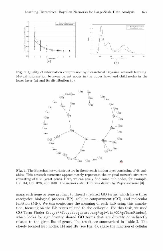
General tendency with respect to the information compression was similar tothe case of synthetic datasets, although not shown here. In the seventh hiddenlayer, consisting of 48 variables, we learned a Bayesian network structure (seeFig. 4). This Bayesian network compactly visualizes the original network struc-ture consisting of 6120 genes. From the network structure, we can easily find aset of hub nodes, e.g., H2, H4, H8, H28, and H30.

Genes comprising these hub nodes and their biological role were analyzed. Thefunction of genes can be described by Gene Ontology (GO) [1] annotations. GO


0 1 2 3 4 5 6 7 80.45

0.5

0.55

0.6

0.65

0.7

0.75

0.8

Hidden layer

Ave

rage

MI b

etw

een

pare

nt a

nd c

hild

nod

esScale−free Bayesian networkModular Bayesian network

(a)

0.5 0.6 0.7 0.8 0.9

02

46

810

1214

MI between parent and child nodes

Den

sity

Scale−free Bayesian networkModular Bayesian network

(b)

Fig. 3. Quality of information compression by hierarchical Bayesian network learning.Mutual information between parent nodes in the upper layer and child nodes in thelower layer (a) and its distribution (b).

H1

H2

H3

H4H5

H6

H7

H8

H9H10

H11

H12

H13

H14

H15

H16

H17H18

H19

H20

H21

H22

H23

H24

H25

H26

H27H28

H29

H30

H31

H32H33

H34

H35H36

H37

H38

H39

H40

H41

H42

H43

H44

H45

H46

H47

H48

Pajek

Fig. 4. The Bayesian network structure in the seventh hidden layer consisting of 48 vari-ables. This network structure approximately represents the original network structureconsisting of 6120 yeast genes. Here, we can easily find some hub nodes, for example,H2, H4, H8, H28, and H30. The network structure was drawn by Pajek software [3].

maps each gene or gene product to directly related GO terms, which have threecategories: biological process (BP), cellular compartment (CC), and molecularfunction (MF). We can conjecture the meaning of each hub using this annota-tion, focusing on the BP terms related to the cell-cycle. For this task, we usedGO Term Finder (http://db.yeastgenome.org/cgi-bin/GO/goTermFinder),which looks for significantly shared GO terms that are directly or indirectlyrelated to the given list of genes. The result are summarized in Table 2. Theclosely located hub nodes, H4 and H8 (see Fig. 4), share the function of cellular

http://db.yeastgenome.org/cgi-bin/GO/goTermFinder


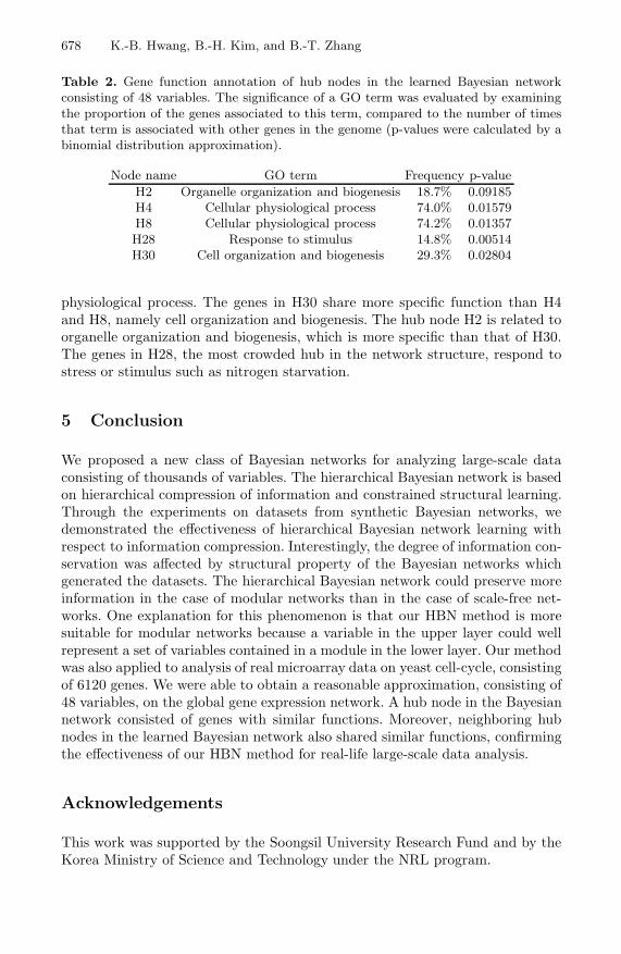
Table 2. Gene function annotation of hub nodes in the learned Bayesian networkconsisting of 48 variables. The significance of a GO term was evaluated by examiningthe proportion of the genes associated to this term, compared to the number of timesthat term is associated with other genes in the genome (p-values were calculated by abinomial distribution approximation).

Node name GO term Frequency p-valueH2 Organelle organization and biogenesis 18.7% 0.09185H4 Cellular physiological process 74.0% 0.01579H8 Cellular physiological process 74.2% 0.01357H28 Response to stimulus 14.8% 0.00514H30 Cell organization and biogenesis 29.3% 0.02804

physiological process. The genes in H30 share more specific function than H4and H8, namely cell organization and biogenesis. The hub node H2 is related toorganelle organization and biogenesis, which is more specific than that of H30.The genes in H28, the most crowded hub in the network structure, respond tostress or stimulus such as nitrogen starvation.

5 Conclusion

We proposed a new class of Bayesian networks for analyzing large-scale dataconsisting of thousands of variables. The hierarchical Bayesian network is basedon hierarchical compression of information and constrained structural learning.Through the experiments on datasets from synthetic Bayesian networks, wedemonstrated the effectiveness of hierarchical Bayesian network learning withrespect to information compression. Interestingly, the degree of information con-servation was affected by structural property of the Bayesian networks whichgenerated the datasets. The hierarchical Bayesian network could preserve moreinformation in the case of modular networks than in the case of scale-free net-works. One explanation for this phenomenon is that our HBN method is moresuitable for modular networks because a variable in the upper layer could wellrepresent a set of variables contained in a module in the lower layer. Our methodwas also applied to analysis of real microarray data on yeast cell-cycle, consistingof 6120 genes. We were able to obtain a reasonable approximation, consisting of48 variables, on the global gene expression network. A hub node in the Bayesiannetwork consisted of genes with similar functions. Moreover, neighboring hubnodes in the learned Bayesian network also shared similar functions, confirmingthe effectiveness of our HBN method for real-life large-scale data analysis.

Acknowledgements

This work was supported by the Soongsil University Research Fund and by theKorea Ministry of Science and Technology under the NRL program.


References

1. Ashburner, M., Ball, C.A., Blake, J.A., Botstein, D., Butler, H., Cherry, J.M.,Davis, A.P., Dolinski, K., Dwight, S.S., Eppig, J.T., Harris, M.A., Hill, D.P., Issel-Tarver, L., Kasarskis, A., Lewis, S., Matese, J.C., Richardson, J.E., Ringwald,M., Rubin, G.M., Sherlock, G.: Gene Ontology: tool for the unification of biology.Nature Genetics 25(1) (2000) 25-29

2. Barabasi, A.-L. and Albert, R.: Emergence of scaling in random networks. Science286(5439) (1999) 509-512

3. Batagelj, V. and Mrvar, A.: Pajek - program for large network analysis. Connec-tions 21(2) (1998) 47-57

4. Friedman, N.: Inferring cellular networks using probabilistic graphical models. Sci-ence 303(6) (2004) 799-805

5. Friedman, N., Nachman, I., Pe’er, D.: Learning Bayesian network structure frommassive datasets: the “sparse candidate” algorithm. Proceedings of the FifteenthConference on Uncertainty in Artificial Intelligence (UAI) (1999) 206-215

6. Goldenberg, A. and Moore, A.: Tractable learning of large Bayes net structuresfrom sparse data. Proceedings of the Twentifirst International Conference on Ma-chine Learning (ICML) (2004)

7. Gyftodimos, E. and Flach, P.: Hierarchical Bayesian networks: an approach to clas-sification and learning for structured data. Lecture Notes in Artificial Intelligence3025 (2004) 291-300

8. Hwang, K.-B., Lee, J.W., Chung, S.-W., Zhang, B.-T.: Construction of large-scaleBayesian networks by local to global search. Lecutre Notes in Artificial Intelligence2417 (2002) 375-384

9. Nikovski, D.: Constructing Bayesian networks for medical diagnosis from incom-plete and partially correct statistics. IEEE Transactions on Knowledge and DataEngineering 12(4) (2000) 509-516

10. Park, S. and Aggarwal, J.K.: Recognition of two-person interactions using a hier-archical Bayesian network. Proceedings of the First ACM SIGMM InternationalWorkshop on Video Surveillance (IWVS) (2003) 65-76

11. Spellman, P.T., Sherlock, G., Zhang, M.Q., Iyer, V.R., Anders, K., Eisen, M.B.,Brown, P.O., Botstein, D., Futcher, B.: Comprehensive identification of cell cycle-regulated genes of the yeast Saccharomyces cerevisiae by microarray hybridization.Molecular Biology of the Cell 9(12) (1998) 3273-3297

lncs 4232 - learning hierarchical bayesian networks for...

Documents