LoadPrediction-basedEnergy-efficientHydraulicActuation

ofaRoboticArm

Miss Can Du, Prof Andrew Plummer and Dr Nigel Johnston

Centre for Power Transmission and Motion Control University of Bath, UK

C.Du@bath.ac.uk

Centre for Power Transmission and Motion Control University of Bath, UK

A.R.Plummer@bath.ac.uk

Centre for Power Transmission and Motion Control University of Bath, UK

D.N.Johnston@bath.ac.uk

In this paper the motion of a two-joint robotic arm is controlled by a variable supply-pressure valve-controlled (VPVC) hydraulic system. It has a fixed capacity pump driven by a brushless servo-motor. The minimum required supply-pressure for the demand motion is predicted. It is computed from the predicted piston force, by applying Lagrange's equations of the-second-kind. The supply-pressure for the whole system is the higher one of the two load branches; the other branch is controlled by throttling. The supply-pressure is varied by controlling motor speed. Simulated and experimental results are shown and discussed. A power consumption comparison with fixed supply-pressure system shows up to 73% saving is found experimentally.

Keywords: Load prediction, energy-efficiency, hydraulic actuation, motion control Target audience: Control System Designers

1 Introduction

In many hydraulic applications, energy efficiency is becoming an important consideration. For a system with multi load branches, one approach is to generate minimum fluid power from the pump: minimum supply pressure or minimum supply flow [1, 2, and 3]. Pump flow should meet exactly the total flow demand with the help of an electronic controller [1]. A method named flow control with indirect feedback was illustrated by Djurovic and Helduser [2]. One primary pressure compensator (PC) instead of a flow sensor is used in each actuator. The method observes whether pump flow is excessive or insufficient via the opening of the PC. A novel power management algorithm for electronic load sensing (ELS) on a telehandler is introduced in [3]. This new ELS algorithm can achieve the advantages of a hydro-mechanical load sensing system: pressure control, flow-sharing, anti-stall, power sharing and prioritization of steering, in the meantime, it can take into account dynamic performance with a load sensing-margin down to 7 bar.

In this paper, a variable pressure valve controlled (VPVC) hydraulic actuation system will be illustrated. It is a hydraulic plant which aims to reduce energy loss by generating a variable supply pressure (PS). The main idea of the VPVC algorithm is to estimate the minimum PS required in advance, thus improving dynamic response. It is similar to load sensing but it does not use any actual pressure signals for control. It predicts the force required by the actuators thus estimating the PS. In addition, it adopts an electronic controller and a servo motor to drive a

fixed displacement pump. This can reduce the weight of plant compared with the traditional load sensing system with a hydraulic controller and a variable displacement pump [4].

A FPVC (fixed supply pressure valve-controlled) hydraulic actuation system has to throttle the flow by the valve to reduce the pressure, which brings an energy loss across the valve. If there are several load branches, the supply pressure should be high enough for all the load branch requirements and all duty cycles.

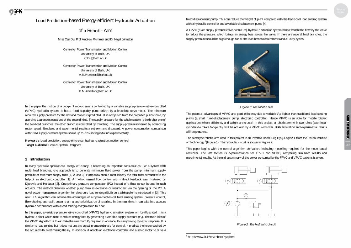
Figure 1: The robotic arm

The potential advantages of VPVC are: good efficiency due to variable PS; lighter than traditional load sensing plants (a small fixed-displacement pump, electronic controller). Hence VPVC is suitable for mobile robotic applications where efficiency and weight are crucial. In this project, a robotic arm with two joints (two linear cylinders to rotate two joints) will be actuated by a VPVC controller. Both simulation and experimental results will be presented.

The prototype robotic arm used in this project is an inverted Robot Leg HyQ-LegV2.1 from the Italian Institute of Technology 1(Figure 1). The hydraulic circuit is shown in Figure 2.

This paper begins with the control algorithm derivation, including modelling required for the model-based controller. The last section is experimentation for FPVC and VPVC, comparing simulated results and experimental results. At the end, a summary of the power consumed by the FPVC and VPVC systems is given.

Figure 2: The hydraulic circuit

1http://www.iit.it/en/robots/hyq.html

2 Controller

The VPVC control algorithm has two parts: feed forward and feedback.

The feed forward is to predict the required minimum PS of the system along with the required spool positions of valves. The calculation can be illustrated by the flow chart in Figure 3. The PS estimated when an individual control valve is fully open is called PSO, and the one to avoid cavitation in the thrust chamber is PSC. PSO and PSC for each actuator are calculated then the actuator with highest required PS is chosen to be master actuator (MA). Its required PS is the final Ps of the whole system. The spool position for the other valve should be computed with this PS. The prediction of PSO and PSC is a crucial problem, which will be discussed in detail in the following section. In this paper, oil compressibility is neglected.

2.1 Supply pressure prediction

2.1.1 Supply pressure required with fully open valve (PSO)

During extension, the return line is connected to the rod side chamber PB and the supply line is connected to the piston side chamber PA. The flow rate demand can be obtained from Q1 = A1 v, Q2 = A2 v; (Q1 is the flow rate into piston side chamber, and Q2 is the flow rate out of the rod side chamber.)

The pressure drops across the valve can be represented as follows:

ASvalve PPP 1 (1)

RBvalve PPP 2 (2)

Then the orifice equation gives:

11 valvePxVKQ (3)

22 valvePxVKQ (4)

If the valve is fully open i.e. x is 100%, and then from Equation (2) and Equation (4) PB can be calculated with an assumption of PR’s value and known KV from the valve’s catalogue.

Figure 3: The flow chart of feed forward in VPVC

FAPAP BA 21 (5)

From Equation (5) PA can be evaluated now.

Finally, back to Equation (1) and Equation (3) the required PS can be estimated.

1

22

1

232

31 )(

APAF

KAvAAP R

VSO

(6)

When retracting, the return line is connected to the piston side PA and the supply line is connected to the rod side chamber PB.

RAvalve PPP 1 (7)

BSvalve PPP 2 (8)

Then using a similar process as for PSO when extending, the PS can be predicted:

2

12

2

232

31 )(

AFPA

KAvAA

P R

VSO

(9)

2.1.2 Supply pressure required to avoid cavitation (PSC)

When extending, PS is connected to PA, which is set to a minimum pressure of Pth (in this project, Pth = 2 bar).

thSvalve PPP 1 (10)

RBvalve PPP 2 (11)

222

21

22

21

2

1

AA

QQ

PP

valve

valve (12)

With the force equation

FAPAP Bth 21 (13)

The value of PS can be calculated:

RthSC PFA

PP 2

2

23 )1(

(14)

The corresponding spool position for the valve to control this MA is computed:

thSCV PPKvAx 1

(15)

When retracting, PS is connected to PB, which is set to a minimum pressure of Pth.

RAvalve PPP 1 (16)

thSvalve PPP 2 (17)

Following the same procedure as for PSC when extending, PS can be predicted:

221

3

1)1

1( R

thSCP

FA

PP (18)

The corresponding spool position for the valve to control this MA is computed:

thSCV PPKvA

x 2 (19)

The final choice of PS = max (PSO1, PSO2, PSC1, PSC2), where subscripts 1 and 2 refer to shoulder actuator and elbow actuator respectively. Hence the spool position of the master actuator (MA) is fully open or for cavitation avoidance is given by Equation (15) or Equation (19). The spool position of the other cylinder is computed by the final value of PS in Equation (20) or Equation (21) below.

2.2 Spool opening of the other cylinder (Non-MA) and motor speed calculation

If the other cylinder is required to extend, its spool opening should be:

=

+

(20)

If the other cylinder is required to retract, its spool opening should be:

=( + )

+

(21)

where xj is the spool position demand of the other cylinder; vj and Fj are its velocity demand and load force respectively; and the area ratio is defined as: / = (22)

When the final PS is determined, given the desired flow rate of each actuator, the required motor speed can be found from Equation (23):

P

jaj

S

m D

QKP

dtd 2

1ˆ

(23)

where K is effective stiffness of the oil inside the supply hoses, and DP is the displacement of pump.

2.3 Required force prediction

From the last section, it is clear that the required force F is required for the PS prediction algorithm. The force is derived by Lagrange equation of the second kind, which incorporates inertia and weight related items.

111

qLLdtd (24)

222

qLLdtd (25)

where VTL , L is the Lagrangian of the system; T is the total kinetic energy and V is the total potential energy of the robotic arm. and are the generalized forces, hence in this case they are the torques required by the shoulder joint and elbow joint respectively. The definitions of and are illustrated in Figure 4.

Figure 4: Geometry of the robotic arm

The results of Equation (24) and Equation (25) are as follows:

= ( + + + + + + + ) + ( + + + ) ( + )( + ) ( + ) ( + ) + ( + ) 2 + ( +

) + 2 (26)

= ( + + + ) + ( + + + ) ( + ) ( + ) + ( +

) + ( + ) (27)

where:

M1 is the mass of upper arm (including elbow cylinder), I1 is its inertia with respect to upper arm gravity centre, through Pm1;

M2 is the mass of forearm (without hand), I2 is its inertia with respect to forearm gravity centre, through Pm2;

M3 is the mass of hand, I3 is its inertia with respect its own gravity centre P3;

L1 is the distance between P1 and P2; L2 is the distance between P2 and P3; C1 is the distance between P1 and Pm1; C2 is the distance between P2 and Pm2.

The actuator force F required is the value of torque computed divided by a lever arm which varies with angular position. Including a viscous damping force, the required hydraulic force prediction for actuators 1 and 2 is:

=( )

+ (28)

=( )

+ (29)

where ( ) and ( ) are the actuator level arm lengths, and B1 and B2 are the damping viscous coefficients.

2.4 Feedback

The measured positions of the actuators are used for feedback. The circumflex (^) represents the output of the feed forward controller. The tilde (~) represents a command signal.

Figure 5: Feedback to motor speed

The position feedback of the MA is used to adjust the motor speed and accordingly the oil flow into the system. There is a proportional-integral (PI) controller multiplied by the sign of MA’s spool position (Figure 5). This method takes into account the direction of the flow imposed by the valve. Hence the motor speed command is:

= m+(KP_M+KI_M

s) yMA sgn( MA) (30)

Actuator position feedback is used to adjust the spool position command of the corresponding valve (Figure 6).

The spool position command is:

= + ( _ + _ )( ) (31)

Figure 6: Feedback to actuator spool position

3 Test Rig and Results

3.1 Test rig schematic

The experiments use an xPC Target real time controller and a NI PCI-6221 data acquisition card. The controller sends out a motor speed command and spool position commands. The joint angular positions are sent back to the controller for feedback (Figure 7). A pressure transducer will be used only for supply pressure observation, not for controller. The measured supply pressure will be compared with the simulated signal and predicted pressure.

Figure 7: Schematic of test rig

The hydraulic system consists of a servo motor which drives a fixed-displacement piston pump. It uses two direct drive valves to control the flow into the cylinders (Figure 8). The components which are being used are as following:

Baldor Brushless AC motor BSM63N-375AF: 2.09 Nm continuous, 8.36 Nm peak, 10000 rpm maximum speed;

Takako micro axial piston pump TFH-315: 3.14 cc/rev, max operating pressure 210 bar, 3000 rpm maximum speed.

Moog Direct Drive valves D633-R02K01M0NSM2: 5 L/min over 35 bar single path pressure drop.

Unequal area actuators: 2.01 cm2/1.23 cm2

For FPVC experiments, a relief valve and a relatively high motor speed command give a constant supply pressure. Only hydraulic power consumed by cylinders ( = _ ) are used in power consumption comparison. For VPVC experiments, the relief valve is set at a high cracking pressure.

Figure 8: The test rig

3.2 Results (simulation and experimentation)

Before experimentation, corresponding simulated tests with sine wave motion demands have been carried out (Table 1). FPVC uses a constant supply pressure of 39 bar in simulation and experimentation. This is found by observing that the spool positions in simulation should be close to fully open for the most demanding duty cycle.

Test No.

Shoulder Demand Elbow Demand FPVC Simulation Information

1 Amp1 = 20o = 3 rad/s Amp2 = 20o = 4 rad/s PS = 39 bar, Max spool opening is 20%

2 Amp1 = 20o = 4 rad/s Amp2 = 20o = 5 rad/s PS = 39 bar, Max spool opening is 35%

3 Amp1 = 30o = 4 rad/s Amp2 = 30o = 5 rad/s PS = 39 bar, Max spool opening is 50%

4 Amp1 = 20o = 7rad/s Amp2 = 30o = 6 rad/s PS = 39 bar, Max spool opening is 75%

5 Amp1 = 30o = 7 rad/s Amp2 = 30o = 7 rad/s PS = 39 bar, Max spool opening is 98%

Table 1: Tests information

Amp1 and Amp2 are the amplitudes of sine wave motion demands for shoulder and elbow respectively; and are corresponding frequencies. For simplicity, only Test 4 (FPVC and VPVC) will be shown and discussed.

Note that and are different frequencies in Test 4.

3.2.1 FPVC results

The position tracking of FPVC (both simulation and experimentation) is shown in Figure 9. The experimental position matches simulated position very well. The supply pressure is fixed at 39 bar. The spool displacement command is shown in Figure 10. The motor speed is commanded to 100 rad/sec i.e. 954 rev/min and is also shown in the figure.

Figure 9: FPVC Test 4 – Angular position tracking and supply pressure tracking

Figure 10: FPVC Test 4 – Valve spool command (-1 to +1) and motor speed

3.2.2 VPVC results

The position tracking and pressure tracking of VPVC is shown (Figure 11). The VPVC control algorithm includes model assumption such as viscous friction, which leads to inevitable errors on hydraulic force prediction, and then on supply pressure prediction. The shoulder motion is slightly affected by elbow motion. But VPVC shows much less lag compared with FPVC position tracking because VPVC predicts the required spool positions while FPVC relies on position feedback control only.

Figure 11: VPVC Test 4 - Angular position tracking and supply pressure tracking

Figure 12: VPVC Test4 –Valve spool command (-1 to +1) and motor speed

The motor speed tracking of VPVC is good (Figure 12). The motor response is very fast with only some transients that the motor cannot track successfully in the experiment (e.g. times 6.73s and 10.32s). In general, the position tracking of VPVC is satisfactory, and experimental pressure tracking and motor speed tracking is good.

3.2.3 Comparison of hydraulic power consumption

The purpose of VPVC is to generate a minimum supply pressure by predicting the force required, and so get a high efficiency compared with a conventional fixed supply pressure system. The hydraulic power of FPVC and VPVC is compared experimentally. The experimental hydraulic power is calculated by velocity (derivative from measured position) and measured supply pressure. The additional power lost through the relief valve with FPVC is not included. From Table 2, it is clear that VPVC can save power among a range of load conditions. The saving increases when the load decreases because FPVC has high waste with low load.

Test No. FPVC Hydraulic Power (W) VPVC Hydraulic Power (W) Saving

(Experimentation)

Simulation Experimentation Simulation Experimentation

1 38.89 38.85 9.31 10.25 73.62%

2 49.44 48.78 15.88 15.87 67.45%

3 77.25 76.57 47.13 41.75 45.47%

4 86.68 86.22 60.11 57.03 33.86%

5 117.59 116.37 104.38 96.10 17.42%

Table 2: Power-Consumption Comparison between FPVC and VPVC

4 Conclusion

From the results of experimentation, it is clear that VPVC is an efficient control method for a multi-axis hydraulic actuation system compared with a traditional industrial fixed supply pressure system. The dynamic performance of VPVC is satisfactory as well, but this is reliant on a highly responsive servomotor. For further improvement, some research on refined feedback control should be carried out, to get a better position tracking.

Nomenclature

Variable Description Unit

PS Supply pressure [bar]

PSO Predicted pressure required with fully open valve [bar]

PSC Predicted pressure required to avoid cavitation [bar]

PR Return pressure [bar]

Pth Threshold pressure to avoid cavitation [bar]

x Spool opening of modulating valve

Area ratio of unequal area cylinder (large area / small area)

q Generalized force for desired motion

I Inertia [kgm2]

MMass of components to robotic arm [kg]

MAMaster actuator

References

/1/ R. Finzel and S. Helduser. Energy-Efficient Electro-Hydraulic Control Systems for Mobile Machinery / Flow Matching. In: 6th International Fluid Power Conference. Dresden. 2008.

/2/ Djurovic, M. and Helduser, S. New Control Strategies for Electrohydraulic Load-Sensing. Power Transmission and Motion Control (PTMC), Bath, 2004.

/3/ Rico. H. Hansen, Torben. O. Andersen and Henrik. C. Pedersen. Development and Implementation of an Advanced Power Management Algorithm for Electronic Load Sensing on a Telehandler. Fluid Power and Motion Control (FPMC), Bath, 2010.

/4/ Marco Scopesi, Prof. Andrew Plummer and Can Du. Energy Efficient Variable Pressure Valve-controlled Hydraulic Actuation. In: Dynamic Systems and Control Conference (DSCC) / Fluid Power and Motion Control (FPMC), Arlington, 2011.