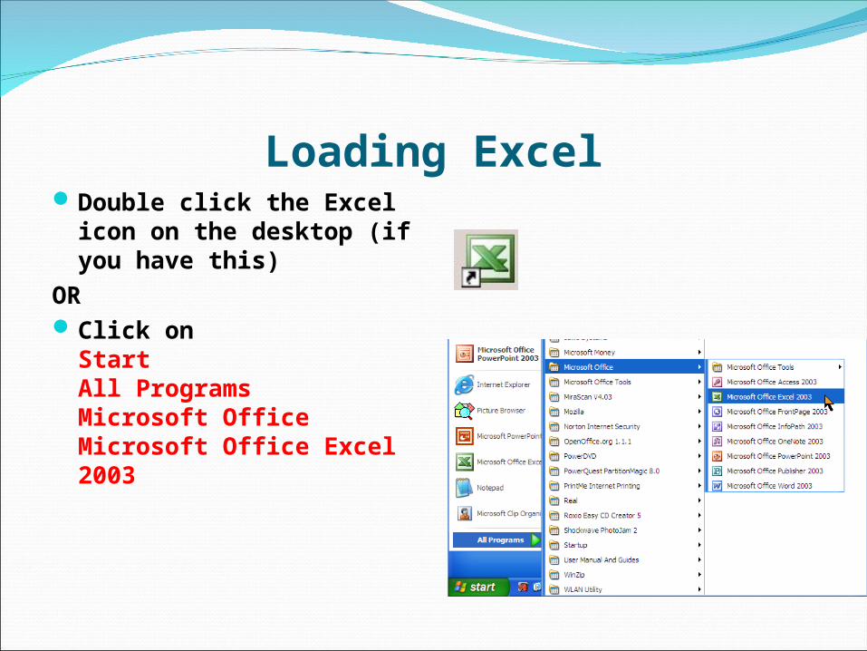
Loading ExcelDouble click the Excel

icon on the desktop (if you have this)

ORClick on

Start All ProgramsMicrosoft OfficeMicrosoft Office Excel 2003

Row

Task Pane

Click here to close the Task PaneActive Cell

Name of Active Cell

Column

Sheet Tabs

Standard ToolbarFormatting Toolbar

What All The Different Parts Mean

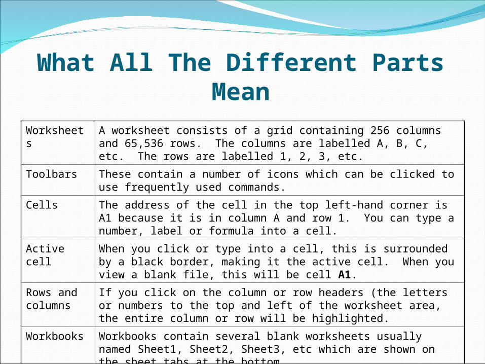
Worksheets

A worksheet consists of a grid containing 256 columns and 65,536 rows. The columns are labelled A, B, C, etc. The rows are labelled 1, 2, 3, etc.

Toolbars These contain a number of icons which can be clicked to use frequently used commands.

Cells The address of the cell in the top left-hand corner is A1 because it is in column A and row 1. You can type a number, label or formula into a cell.

Active cell When you click or type into a cell, this is surrounded by a black border, making it the active cell. When you view a blank file, this will be cell A1.

Rows and columns

If you click on the column or row headers (the letters or numbers to the top and left of the worksheet area, the entire column or row will be highlighted.

Workbooks Workbooks contain several blank worksheets usually named Sheet1, Sheet2, Sheet3, etc which are shown on the sheet tabs at the bottom.

Task pane This area lists workbooks recently opened and other options. You can close this by clicking on the Close icon in the top right hand corner.

Entering Data

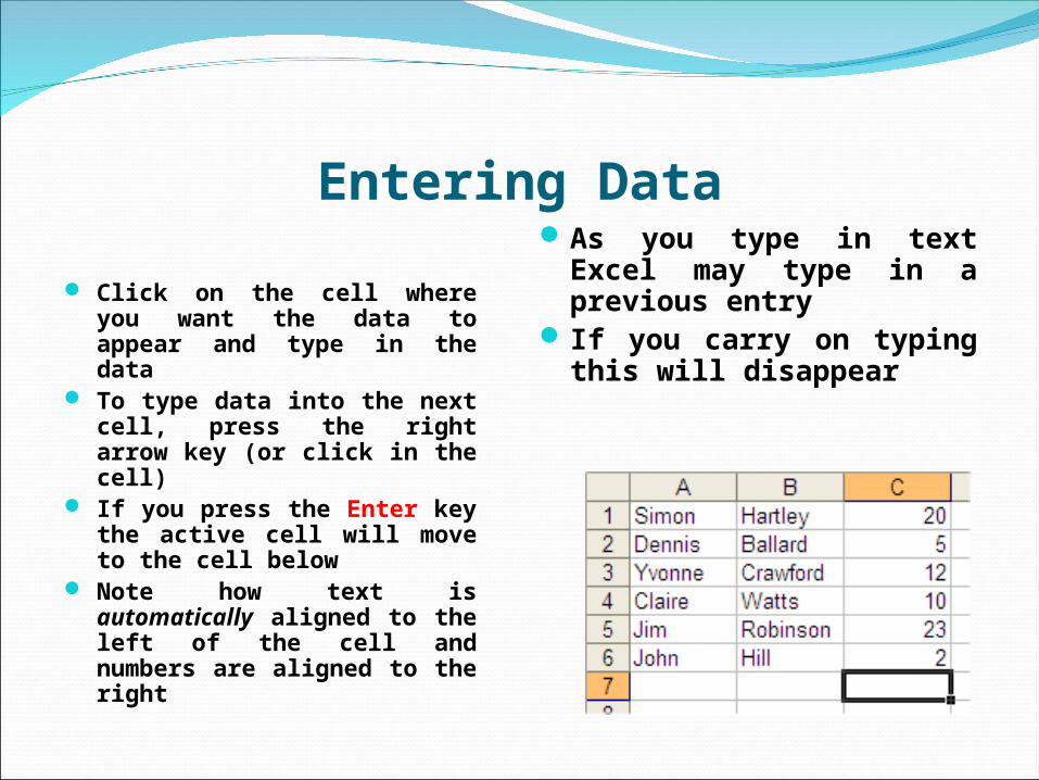
Click on the cell where you want the data to appear and type in the data

To type data into the next cell, press the right arrow key (or click in the cell)

If you press the Enter key the active cell will move to the cell below

Note how text is automatically aligned to the left of the cell and numbers are aligned to the right

As you type in text Excel may type in a previous entry

If you carry on typing this will disappear

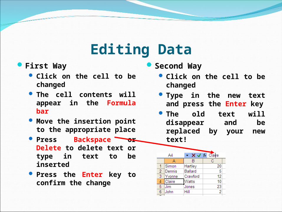
Editing DataFirst Way

Click on the cell to be changed

The cell contents will appear in the Formula bar

Move the insertion point to the appropriate place

Press Backspace or Delete to delete text or type in text to be inserted

Press the Enter key to confirm the change

Second Way Click on the cell to be

changed Type in the new text and

press the Enter key The old text will

disappear and be replaced by your new text!

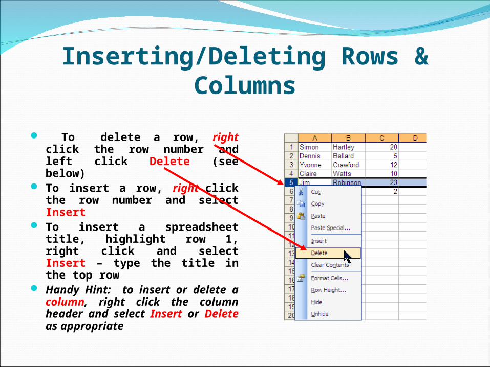
Inserting/Deleting Rows & Columns

To delete a row, right click the row number and left click Delete (see below)

To insert a row, right click the row number and select Insert

To insert a spreadsheet title, highlight row 1, right click and select Insert – type the title in the top row

Handy Hint: to insert or delete a column, right click the column header and select Insert or Delete as appropriate

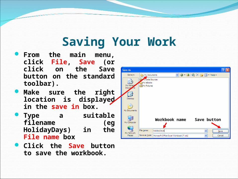
Saving Your Work From the main menu,

click File, Save (or click on the Save button on the standard toolbar).

Make sure the right location is displayed in the save in box.

Type a suitable filename (eg HolidayDays) in the File name box

Click the Save button to save the workbook.

Workbook name Save button

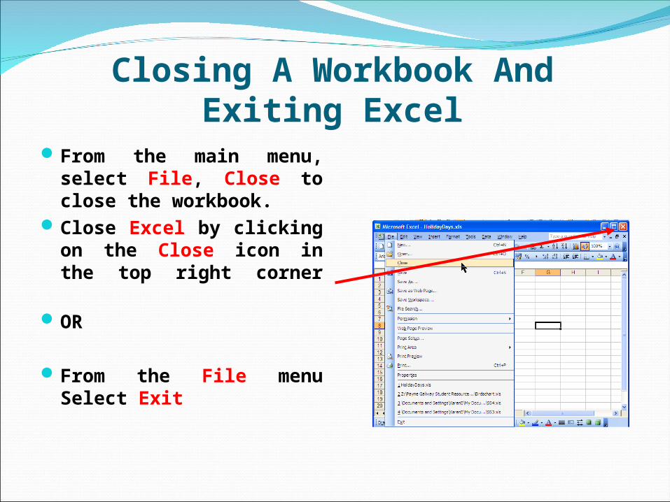
Closing A Workbook And Exiting Excel

From the main menu, select File, Close to close the workbook.

Close Excel by clicking on the Close icon in the top right corner

OR

From the File menu Select Exit

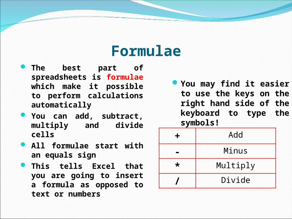
Formulae

+ Add

- Minus

* Multiply

/ Divide

The best part of spreadsheets is formulae which make it possible to perform calculations automatically

You can add, subtract, multiply and divide cells

All formulae start with an equals sign

This tells Excel that you are going to insert a formula as opposed to text or numbers

You may find it easier to use the keys on the right hand side of the keyboard to type the symbols!

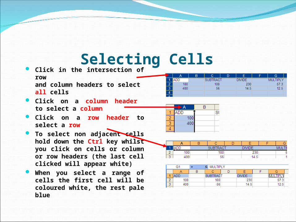
Selecting Cells Click in the intersection of

row and column headers to select

all cells Click on a column header

to select a column Click on a row header to

select a row To select non adjacent cells

hold down the Ctrl key whilst you click on cells or column or row headers (the last cell clicked will appear white)

When you select a range of cells the first cell will be coloured white, the rest pale blue

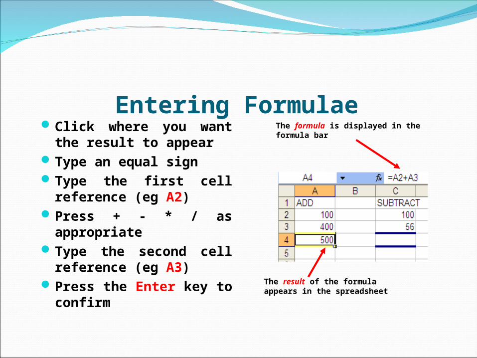
Entering FormulaeClick where you want

the result to appearType an equal signType the first cell

reference (eg A2)Press + - * / as

appropriateType the second cell

reference (eg A3)Press the Enter key to

confirm

The result of the formula appears in the spreadsheet

The formula is displayed in the formula bar

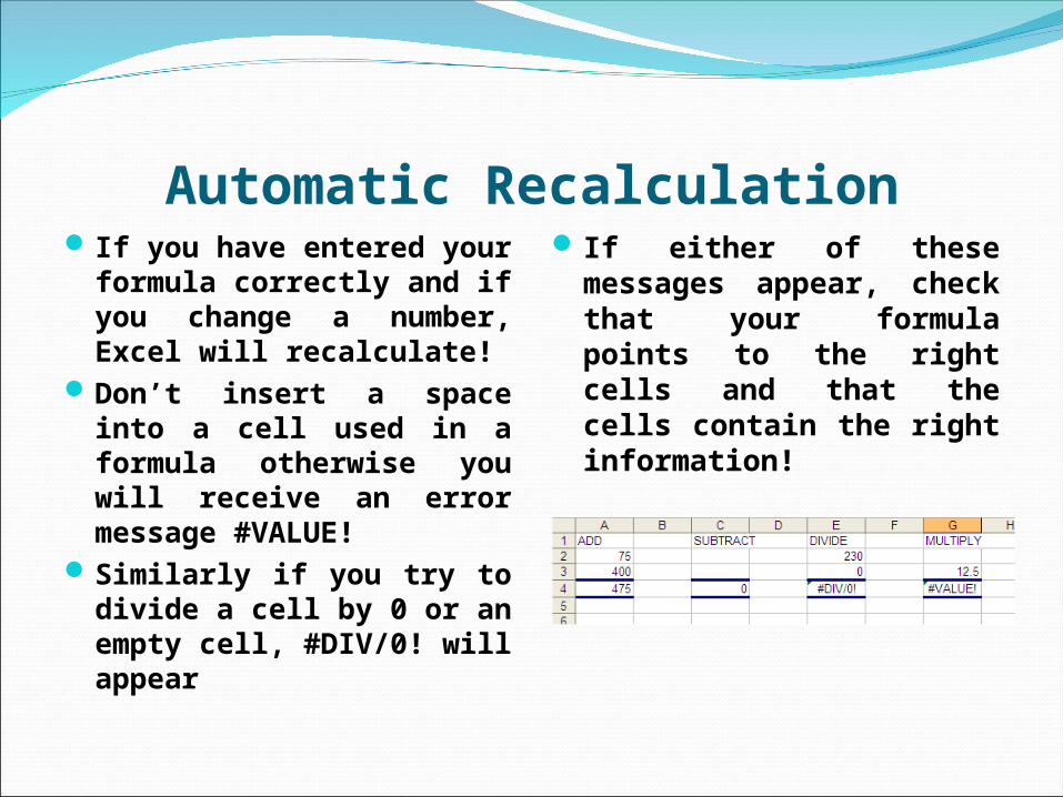
Automatic RecalculationIf you have entered your

formula correctly and if you change a number, Excel will recalculate!

Don’t insert a space into a cell used in a formula otherwise you will receive an error message #VALUE!

Similarly if you try to divide a cell by 0 or an empty cell, #DIV/0! will appear

If either of these messages appear, check that your formula points to the right cells and that the cells contain the right information!

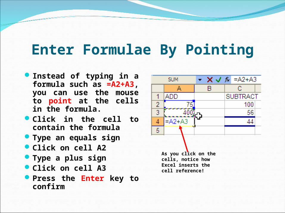
Enter Formulae By Pointing

Instead of typing in a formula such as =A2+A3, you can use the mouse to point at the cells in the formula.

Click in the cell to contain the formula

Type an equals signClick on cell A2Type a plus signClick on cell A3Press the Enter key to

confirm

As you click on the cells, notice how Excel inserts the cell reference!

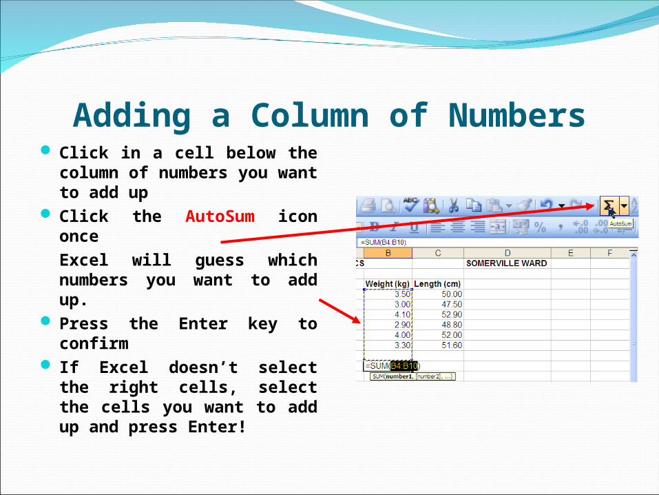
Adding a Column of Numbers Click in a cell below the

column of numbers you want to add up

Click the AutoSum icon onceExcel will guess which numbers you want to add up.

Press the Enter key to confirm

If Excel doesn’t select the right cells, select the cells you want to add up and press Enter!

FunctionsA function is a formula

used in a calculationExcel has over 200

functions to help with many applications

You will learn about: =SUM =AVERAGE =MIN =MAX =COUNT

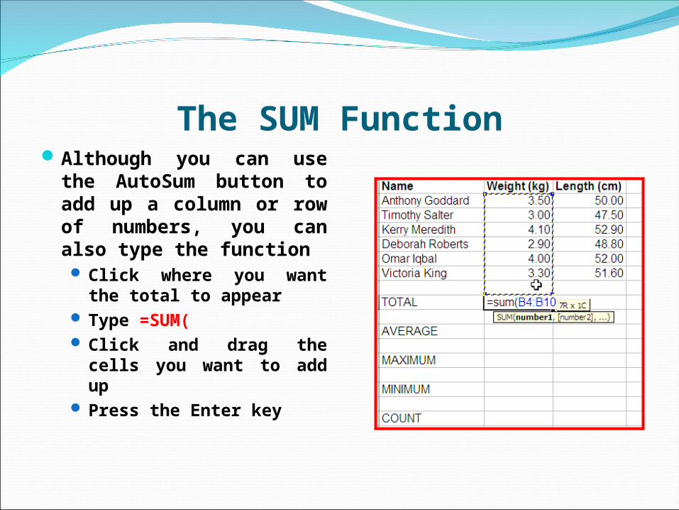
The SUM FunctionAlthough you can use

the AutoSum button to add up a column or row of numbers, you can also type the function Click where you want

the total to appear Type =SUM( Click and drag the cells

you want to add up Press the Enter key

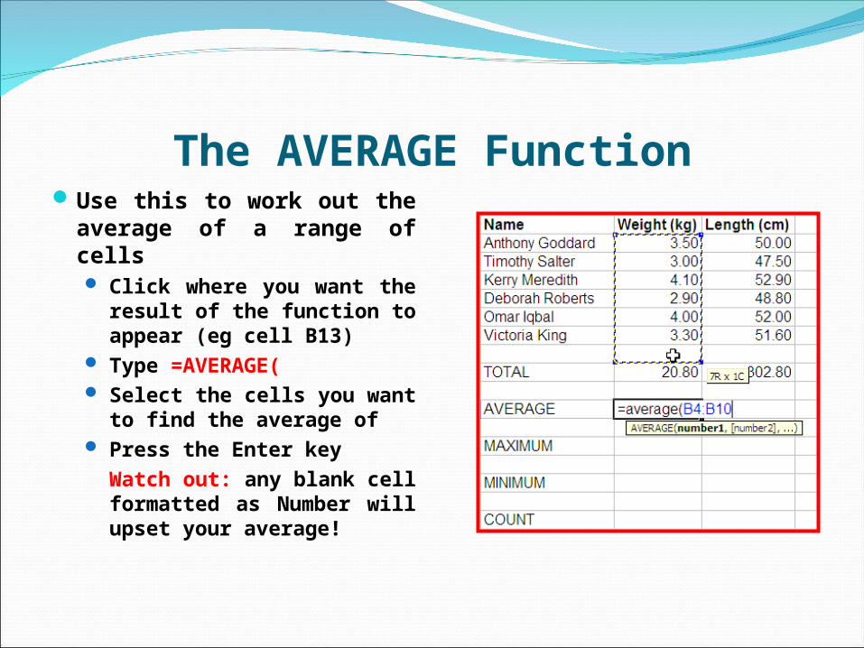
The AVERAGE FunctionUse this to work out the

average of a range of cells Click where you want

the result of the function to appear (eg cell B13)

Type =AVERAGE( Select the cells you want

to find the average of Press the Enter key

Watch out: any blank cell formatted as Number will upset your average!

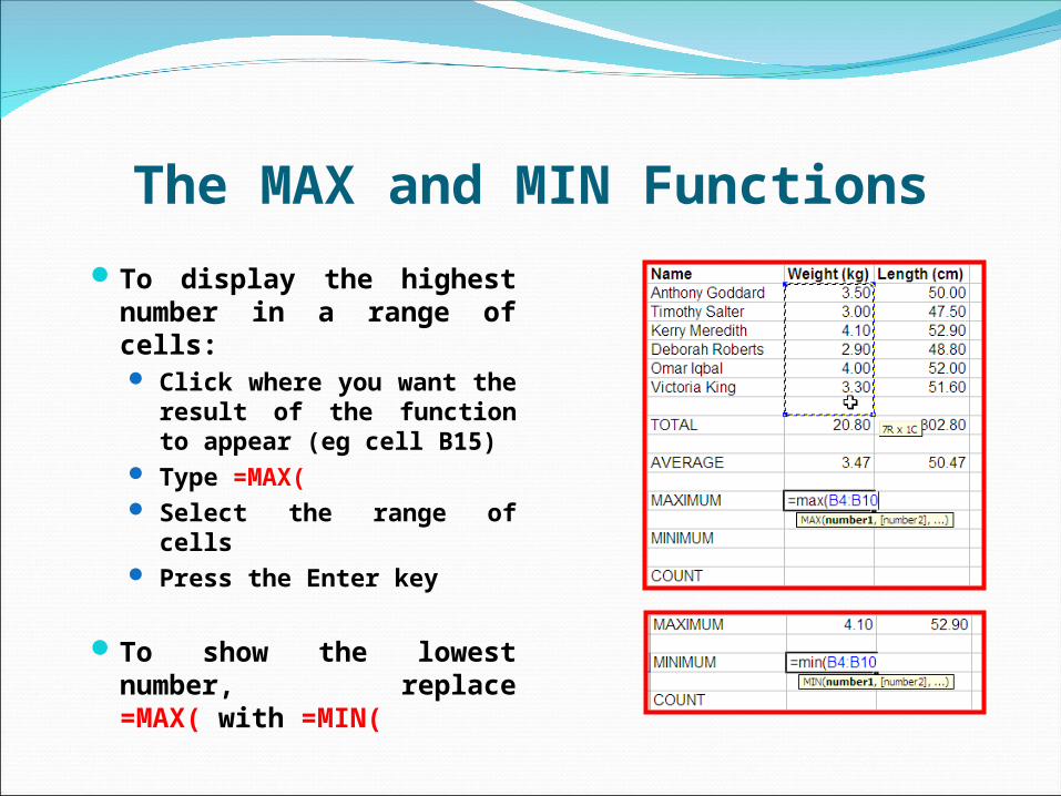
The MAX and MIN Functions

To display the highest number in a range of cells: Click where you want

the result of the function to appear (eg cell B15)

Type =MAX( Select the range of cells Press the Enter key

To show the lowest number, replace =MAX( with =MIN(

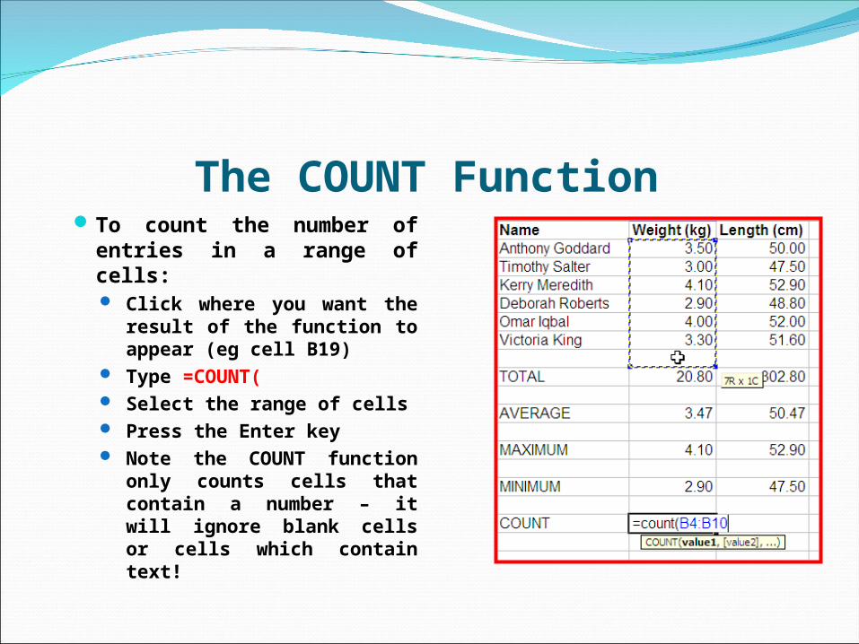
The COUNT FunctionTo count the number of

entries in a range of cells: Click where you want the

result of the function to appear (eg cell B19)

Type =COUNT( Select the range of cells Press the Enter key Note the COUNT function

only counts cells that contain a number – it will ignore blank cells or cells which contain text!

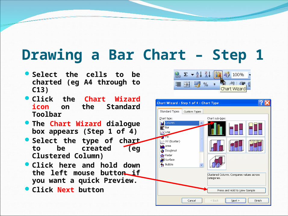
Drawing a Bar Chart – Step 1Select the cells to be

charted (eg A4 through to C13)

Click the Chart Wizard icon on the Standard Toolbar

The Chart Wizard dialogue box appears (Step 1 of 4)

Select the type of chart to be created (eg Clustered Column)

Click here and hold down the left mouse button if you want a quick Preview.

Click Next button

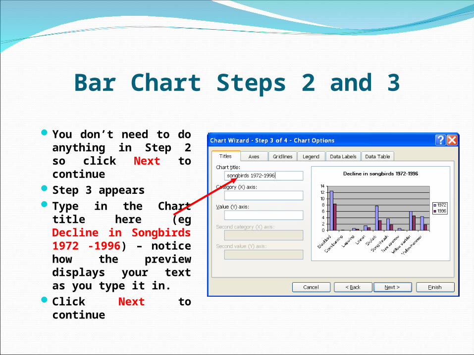
Bar Chart Steps 2 and 3

You don’t need to do anything in Step 2 so click Next to continue

Step 3 appearsType in the Chart

title here (eg Decline in Songbirds 1972 -1996) – notice how the preview displays your text as you type it in.

Click Next to continue

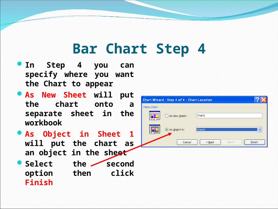
Bar Chart Step 4In Step 4 you can specify

where you want the Chart to appear

As New Sheet will put the chart onto a separate sheet in the workbook

As Object in Sheet 1 will put the chart as an object in the sheet

Select the second option then click Finish

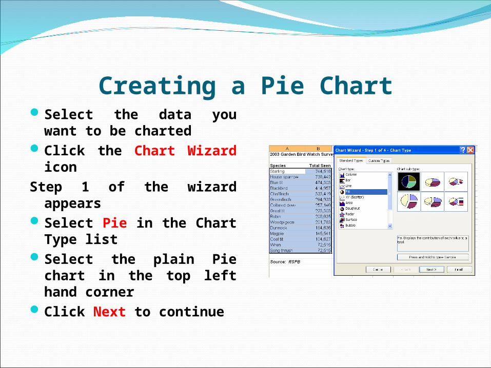
Creating a Pie ChartSelect the data you want

to be chartedClick the Chart Wizard

iconStep 1 of the wizard

appearsSelect Pie in the Chart

Type listSelect the plain Pie

chart in the top left hand corner

Click Next to continue

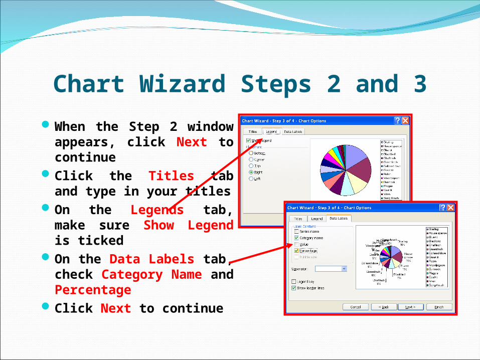
Chart Wizard Steps 2 and 3

When the Step 2 window appears, click Next to continue

Click the Titles tab and type in your titles

On the Legends tab, make sure Show Legend is ticked

On the Data Labels tab, check Category Name and Percentage

Click Next to continue

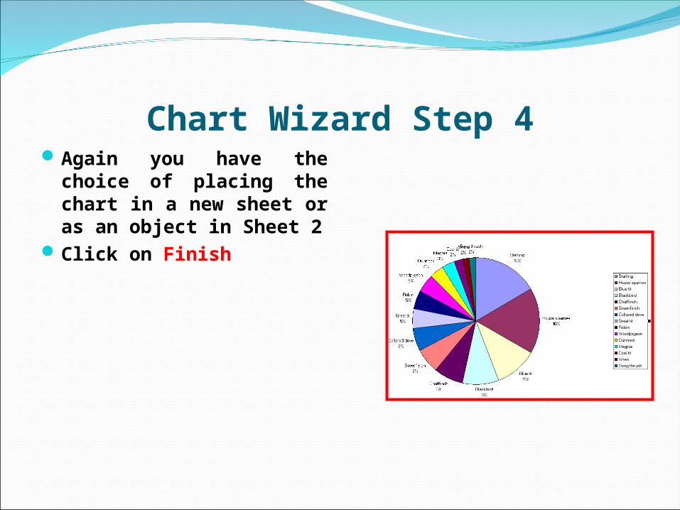
Chart Wizard Step 4Again you have the

choice of placing the chart in a new sheet or as an object in Sheet 2

Click on Finish