local asymptotic minimax estimation of ......local asymptotic minimax estimation of nonregular...

LOCAL ASYMPTOTIC MINIMAX ESTIMATION OF NONREGULARPARAMETERS WITH TRANSLATION-SCALE EQUIVARIANT MAPS

KYUNGCHUL SONG

Abstract. When a parameter of interest is de�ned to be a nondi¤erentiable transformof a regular parameter, the parameter does not have an in�uence function, renderingthe existing theory of semiparametric e¢ cient estimation inapplicable. However, whenthe nondi¤erentiable transform is a known composite map of a continuous piecewiselinear map with a single kink point and a translation-scale equivariant map, this paperdemonstrates that it is possible to de�ne a notion of asymptotic optimality of an esti-mator as an extension of the classical local asymptotic minimax estimation. This paperestablishes a local asymptotic risk bound and proposes a general method to constructa local asymptotic minimax decision.

Key words. Nonregular Parameters; Translation-Scale Equivariant Transforms; Semi-parametric E¢ ciency; Local Asymptotic Minimax Estimation.

AMS Classification. 62C05, 62C20.

1. Introduction

This paper investigates the problem of optimal estimation of a parameter � 2 R whichtakes the following form:

(1.1) � = (f � g)(�);where � 2 Rd is a regular parameter for which a semiparametric e¢ ciency bound is wellde�ned, g is a translation-scale equivariant map, and f is a continuous piecewise linearmap with a single kink point.Examples abound, including maxf�1; �2; �3g, maxf�1; 0g, j�1j, jmaxf�1; �2gj, etc.,

where � = (�1; �2; �3) is a regular parameter, i.e., a parameter which is di¤erentiablein the underlying probability. For example, one might be interested in the absolutedi¤erence between two conditional means � = jE[Y jX = x1]� E[Y jX = x2]j ; or themaximum between two di¤erent treatment e¤ects � = max1�j�J �j with �j = E[Y jX =x;D = j] � E[Y jX = x;D = 0], where Y is an outcome variable, D 2 f0; 1; � � �; Jgtreatment type (with 0 representing no treatment), and X is a discrete covariate vector.Another example involves the object of interest bounded by unknown quantities �1 and�2, forming a common bound minf�1; �2g. Such a bound frequently arises in economicsliterature (e.g. Manski and Pepper (2000) for returns to education and Haile and Tamer(2003) for bidders�valuations in English auctions.)In contrast to the ease with which such parameters arise in applied researches, a

formal analysis of the optimal estimation problem has remained a challenging task. One

Date: December 29, 2012.1

2 K. SONG

might consistently estimate � by using plug-in estimator � = f(g(�)), where � is apn-

consistent estimator of �. However, there have been concerns about the asymptotic biasthat such an estimator carries, and some researchers have proposed ways to reduce thebias (Manski and Pepper (2000), Haile and Tamer (2003), Chernozhukov, Lee, and Rosen(2010)). However, Doss and Sethuraman (1989) showed that a sequence of estimatorsof a parameter for which there is no unbiased estimator must have variance diverging toin�nity if the bias decreases to zero. (See also Hirano and Porter (2010) for a recent resultfor nondi¤erentiable parameters.) Given that one cannot eliminate the bias entirelywithout its variance exploding, the bias reduction may do the estimator either harm orgood.Many early researches on estimation of a nonregular parameter considered a paramet-

ric model and focused on �nite sample optimality properties. For example, estimation ofa normal mean under bound restrictions or order restrictions has been studied, amongmany others, by Lovell and Prescott (1970), Casella and Strawderman (1981), Bickel(1981), Moors (1981), and more recently van Eeden and Zidek (2004). Closer to thispaper are researches by Blumenthal and Cohen (1968a,b) who studied estimation ofmaxf�1; �2g; when i.i.d. observations from a location family of symmetric distributionsor normal distributions are available. On the other hand, the notion of asymptotic ef-�cient estimation through the convolution theorem and the local asymptotic minimaxtheorem initiated by Hajék (1972) and Le Cam (1979) has mostly focused on regularparameters, and in many cases, resulted in regular estimators as optimal estimators.Hence the classical theory of semiparametric estimation widely known and well sum-marized in monographs such as Bickel, Klassen, Ritov, and Wellner (1993) and in laterchapters of van der Vaart and Wellner (1996) does not directly apply to the problem ofestimation of � = (f � g)(�). This paper attempts to �ll this gap from the perspectiveof local asymptotic minimax estimation.This paper �nds that for the class of nonregular parameters of the form (1.1), we

can extend the existing theory of local asymptotic minimax estimation and construct areasonable class of optimal estimators that are nonregular in general and asymptoticallybiased. The class of optimal estimators take the form of a plug-in estimator with semi-parametrically e¢ cient estimator of � except that it involves an additive bias-adjustmentterm which can be computed using simulations.To deal with nondi¤erentiability, this paper �rst focuses on the special case where f

is an identity, and utilizes the approach of generalized convolution theorem in van derVaart (1989) to establish the local asymptotic minimax risk bound for the parameter �.However, such a risk bound is hard to use in our set-up where f or g is potentially asym-metric, because the risk bound involves minimization of the risk over the distributionsof �noise� in the convolution theorem. This paper uses the result of Dvoretsky, Wald,and Wolfowitz (1951) to reduce the risk bound to one involving minimization over areal line. And then this paper proposes a local asymptotic minimax decision of a simpleform:

g(�) + c=pn;

where � is a semiparametrically e¢ cient estimator of � and c is a bias adjustment termthat can be computed through simulations.

OPTIMAL ESTIMATION OF NONREGULAR PARAMETERS 3

Next, extension to the case where f is continuous piecewise linear with a single kinkpoint is done by making use of the insights of Blumenthal and Cohen (1968a) andapplying them to local asymptotic minimax estimation. Thus, an estimator of the form

(1.2) �mx � f�g(�) +

cpn

�;

with appropriate bias adjustment term c, is shown to be local asymptotic minimax. Inseveral situations, the bias adjustment term c can be set to zero. In particular, when� = s0�, for some known vector s 2 Rd, so that � is a regular parameter, the biasadjustment term can be set to be zero, and an optimal estimator in (1.2) is reduced tos0� which is a semiparametric e¢ cient estimator of � = s0�. This con�rms the continuityof this paper�s approach with the standard method of semiparametric e¢ ciency.This paper o¤ers results from a small sample simulation study for the cases of � =

maxf�1; �2g and � = maxf0; �2g, where the bias adjustment suggested by the localasymptotic minimax estimation is either not necessary or only very minimal. This papercompares the method with two alternative bias reduction methods: �xed bias reductionmethod and a selective bias reduction method. The method of local asymptotic minimaxestimation shows relatively robust performance in terms of the �nite sample risk.The next section de�nes the scope of the paper by introducing nondi¤erentiable trans-

forms that this paper focuses on. The section also introduces regularity conditions forprobabilities that identify �. Section 3 investigates optimal decisions based on the lo-cal asymptotic maximal risks. Section 4 presents and discusses Monte Carlo simulationresults. All the mathematical proofs are relegated to the Appendix.We introduce some notation. Let N be the collection of natural numbers. Let 1d be

a d� 1 vector of ones with d � 2. For a vector x 2 Rd and a scalar c, we simply writex+ c = x+ c1d, or write x = c instead of x = c1d. We de�ne S1 � fx 2 Rd : x01d = 1g,where the notation � indicates de�nition. For x 2 Rd, the notation max(x) (or min(x))means the maximum (or the minimum) over the entries of the vector x. When x1; � � �; xnare scalars, we also use the notationsmaxfx1; ��; xng andminfx1; ��; xng whose meaningsare obvious. We let �R = [�1;1] and view it as a two-point compacti�cation of R, andlet �Rd be the product of its d copies.

2. Nondifferentiable Transforms of a Regular Parameter

As for the parameter of interest �, this paper assumes that

(2.1) � = (f � g)(�);

where � 2 Rd is a regular parameter (the meaning of regularity for � is clari�ed inAssumption 3 below), and g : �Rd ! �R and f : �R! �R satisfy the following assumptions.

Assumption 1: (i) The map g : �Rd ! �R is Lipschitz continuous, g(Rd) � R, andsatis�es the following.(a) (Translation Equivariance) For each c 2 �R and x 2 Rd, g(x+ c) = g(x) + c:(b) (Scale Equivariance) For each u � 0 and x 2 Rd; g(ux) = ug(x):(ii) The map f : �R! �R is continuous, piecewise linear with one kink at a point in R.

4 K. SONG

Assumption 1 essentially de�nes the scope of this paper. Some examples of g are asfollows.

Examples 1: (a) g(x) = s0x; where s 2 S1.(b) g(x) = max(x) or g(x) = min(x).(c) g(x) = maxfmin(x1);x2g, g(x) = max(x1) + max(x2); g(x) = min(x1) + min(x2);g(x) = max(x1) + min(x2); or g(x) = max(x1) + s0x with s 2 S1, where x1 and x2 aresubvectors of x.

One might ask whether the representation of parameter � as a composition map f � gof � in (2.1) is unique. The following lemma gives an a¢ rmative answer.

Lemma 1: Suppose that f1 and f2 are R-valued maps on R that are non-constant onR, and g1 and g2 satisfy Assumption 1(i). If f1 � g1 = f2 � g2; we have

f1 = f2 and g1 = g2.

As we shall see later, the local asymptotic minimax risk bound involves g and theoptimal estimators involve the maps f and g. The uniqueness result of Lemma 1 removesambiguity that could potentially arise when � had multiple equivalent representationswith di¤erent maps f and g.We introduce brie�y conditions for probabilities that identify �, in a manner adapted

from van der Vaart (1991) and van der Vaart and Wellner (1996). Let P � fP� : � 2 Agbe a family of distributions on a measurable space (X ;G) indexed by � 2 A, where theset A is a subset of a Euclidean space or an in�nite dimensional space. We assume thatwe have i.i.d. draws Y1; � � �; Yn from P�0 2 P so that Xn � (Y1; � � �; Yn) is distributed asP n�0. Let P(P�0) be the collection of maps t! P�t such that for some h 2 L2(P�0),Z �

1

t

�dP 1=2�t � dP

1=2�0

�� 12hdP 1=2�0

�2! 0; as n!1:

When this convergence holds, we say that P�t converges in quadratic mean to P�0 , callh 2 L2(P�0) a score function associated with this convergence, and call the set of allsuch h�s a tangent set, denoting it by T (P�0): We assume that the tangent set is alinear subspace of L2(P�0). Taking h�; �i to be the usual inner product in L2(P�0), wewrite H � T (P�0) and view (H; h�; �i) as a subspace of a separable Hilbert space, with�H denoting its completion. For each h 2 H; n 2 N, and �h 2 A; let P�0+�h=pn beprobabilities converging in quadratic mean to P�0 as n!1 having h as its associatedscore. We simply write Pn;h = P n

�0+�h=pnand consider sequences of such probabilities

fPn;hgn�1 indexed by h 2 H. (See van der Vaart (1991) and van der Vaart and Wellner(1996), Section 3.11 for details.) The collection En � (Xn;Gn; Pn;h;h 2 H) constitutes asequence of statistical experiments for � (Blackwell (1951)). As for En, we assume localasymptotic normality as follows.

Assumption 2: (Local Asymptotic Normality) For each h 2 H,

logdPn;hdPn;0

= �n(h)�1

2hh; hi;


where for each h 2 H, �n(h) �(h) (weak convergence under fPn;0g) and �(�) is acentered Gaussian process on H with covariance function E[�(h1)�(h2)] = hh1; h2i:

Local asymptotic normality reduces the decision problem to one in which an optimaldecision is sought under a single Gaussian shift experiment E = (X ;G; Ph;h 2 H); wherePh is such that log dPh=dP0 = �(h)� 1

2hh; hi: The local asymptotic normality is ensured,

for example, when Pn;h = P nh and Ph is Hellinger-di¤erentiable (Begun, Hall, Huang,and Wellner (1983).) The space H is a tangent space for � associated with the spaceof probability sequences ffPn;hgn�1 : h 2 Hg (van der Vaart (1991).) Taking � as anRd-valued map on fPn;h : h 2 Hg, we can regard the map as a sequence of Rd-valuedmaps on H and write it as �n(h).

Assumption 3: (Regular Parameter) There exists a continuous linear Rd-valued map,_�, on H such that p

n(�n(h)� �n(0))! _�(h)

as n!1:

Assumption 3 requires that �n(h) is regular in the sense of van der Vaart and Wellner(1996, Section 3.11). The map _� in Assumption 3 is associated with the semiparametrice¢ ciency bound of �. For each b 2 Rd, b0 _�(�) de�nes a continuous linear functionalon H, and hence there exists _�

�b 2 �H such that b0 _�(h) = h _��b; hi; h 2 H. Then for any

b 2 Rd, jj _��bjj2 represents the asymptotic variance bound of the parameter b0�. Themap _�

�b is called an e¢ cient in�uence function for b

0� in the literature (e.g. van derVaart (1991)). Let em be a d� 1 vector whose m-th entry is one and the other entriesare zero, and let � be a d � d matrix whose (m; k)-th entry is given by h _��em ; _�

�eki. As

for �, we assume the following:

Assumption 4: � is invertible.

The inverse of matrix � is called the semiparametric e¢ ciency bound for �: In particular,Assumption 4 requires that there is no redundancy among the entries of �, i.e., one entryof � is not de�ned as a linear combination of the other entries.

3. Local Asymptotic Minimax Estimators

3.1. Loss Functions. For a decision d 2 R and the object of interest � 2 R, we considerthe following form of a loss function:

(3.1) L (d; �) = �(jd� �j);where � : R! R is a map that satis�es the following assumption.

Assumption 5: �(�) is nonnegative, strictly increasing, �(y)!1 as y !1, �(0) = 0,and for each M > 0, there exists cM > 0 such that for all x; y 2 R,

j�M(x)� �M(y)j � cM jx� yj;where �M(�) = minf�(�);Mg.

6 K. SONG

While Assumption 5 is satis�ed by many loss functions, it excludes the hypothesistesting type loss function �(jd � �j) = 1fjd � �j > cg, c 2 R. The following lemmaestablishes a lower bound for the local asymptotic minimax risk when f is an identity.Let Z 2 Rd be a random vector having distribution equal to N(0;�).

Lemma 2: Suppose that Assumptions 1-5 hold. Then for any sequence of estimators �,

liminfn!1

suph2H

Eh

h�(jpnf� � g(�n(h))gj)

i� inf

F2Fsupr2Rd

ZE [�(jg(Z + r)� g(r) + wj)] dF (w);

where F denotes the collection of probability measures on the Borel �-�eld of R.

The lemma establishes a lower bound for the risk. The result is obtained by using aversion of a generalized convolution theorem in van der Vaart (1989) which is adaptedto the current set-up. The main di¢ culty with Lemma 2 is that the supremum overr 2 Rd and the in�mum over F 2 F do not have an explicit solution in general. Hencethis paper considers simulating the lower bound in Lemma 2 by using random drawsfrom a distribution approximating that of Z. The main obstacle in this approach is thatthe risk lower bound involves in�mum over an in�nite dimensional space F .We obtain a much simpler formulation by using the classical puri�cation result of

Dvoretsky, Wald, and Wolfowitz (1951) for zero sum games, where it is shown that therisk of a randomized decision can be replaced by that of a nonrandomized decision whenthe distributions of observations are atomless. This result has had an impact on theliterature of puri�cations in incomplete information games (e.g. Milgrom and Weber(1985)). In our set-up, the observations are not drawn from an atomless distribution,but in the limiting experiment, we can regard them as drawn from a shifted normaldistribution. This enables us to use their result to obtain the following theorem.

Theorem 1: Suppose that Assumptions 1-5 hold. Then for any sequence of estimators�,

liminfn!1

suph2H

Eh

h�(jpnf� � g(�n(h))gj)

i� inf

c2RB(c; 1);

where for c 2 R, and a � 0;

B(c; a) � supr2Rd

E [�(ajg(Z + r)� g(r) + cj)] :

The main feature of the lower bound in Theorem 1 is that it involves in�mum over asingle-dimensional space R in its risk bound. This simpler form now makes it feasibleto simulate the lower bound for the risk.This paper proposes a method of constructing a local asymptotic minimax estimator

as follows. Suppose that we are given a consistent estimator � of � and a semiparamet-rically e¢ cient estimator � of � which satisfy the following assumptions. (See Bickel,Klaasen, Ritov, and Wellner (1993) for semiparametric e¢ cient estimators from variousmodels.)


Assumption 6: (i) For each " > 0, there exists a > 0 such that

limsupn!1suph2HPn;hfpnjj�� jj > ag < ":

(ii) For each t 2 Rd, suph2H��Pn;hfpn(� � �n(h)) � tg � PfZ � tg��! 0 as n!1.

Assumption 6 imposespn-consistency of � and convergence in distribution of

pn(��

�n(h)); both uniform over h 2 H. The uniform convergence can be proved through thecentral limit theorem uniform in h 2 H. Under regularity conditions, the uniform centrallimit theorem of a sum of i.i.d. random variables follows from a Berry-Esseen bound, aslong as the third moment of the random variable is bounded uniformly in h 2 H:For technical facility, we follow a suggestion by Strasser (1985) (p.440) and consider

a truncated loss: �M(�) = minf�(�);Mg for large M: To simulate the risk lower boundin Theorem 1, we �rst draw f�igLi=1 i.i.d. from N(0; Id). For a �xed large M1 > 0; let

BM1(c; 1) � supr2[�M1;M1]d

1

L

LXi=1

�M1

�jg(�1=2�i + r)� g(r) + cj

�.

Then we obtain

(3.2) cM1 �1

2

nsup EM1 + inf EM1

o;

where, with �n;L ! 0 as n; L ! 1, �n;Lpn ! 1 as n ! 1 and �n;L

pL ! 1 as

L!1,

EM1 ��c 2 [�M1;M1] : BM1(c; 1) � inf

c12[�M1;M1]BM1(c1; 1) + �n;L

�:

Let us construct

(3.3) �mx � g(�) +cM1pn:

The following theorem a¢ rms that �mx is local asymptotic minimax for � = g(�).

Theorem 2: Suppose that the conditions of Theorem 1 and Assumption 6 hold. Then,

limM1�M :M"1

limsupn!1

suph2H

Eh

h�M(j

pnf�mx � g(�n(h))gj)

i� inf

c2RB(c; 1):

Recall that the candidate estimators considered in Theorem 1 were not restricted toplug-in estimators with an additive bias adjustment term. As standard in the literatureof local asymptotic minimax estimation, the candidate estimators are any sequences ofmeasurable functions of observations including both regular and nonregular estimators.The main thrust of Theorem 2 is the �nding that it is su¢ cient for local asymptoticminimax estimation to consider a plug-in estimator using a semiparametrically e¢ cientestimator of � with an additive bias adjustment term as in (3.3). It remains to �ndoptimal bias adjustment, which can be done using the simulation method proposedearlier.We now extend the result to the case where f is not an identity map, but a continuous

piecewise linear map with a single kink point. The main idea is taken from the proof ofTheorem 3.1 of Blumenthal and Cohen (1968a).

8 K. SONG

Theorem 3: Suppose that the conditions of Theorem 1 hold, and let s be the maximumabsolute slope from the two linear components of f . Then for any sequence of estimators�,

liminfn!1

suph2H

Eh

h�(jpnf� � (f � g)(�n(h))gj)

i� inf

c2RB(c; s):

The bounds in Theorems 1 and 3 involve a bias adjustment term c� that minimizesB(c; 1). A similar bias adjustment term appears in Takagi (1994)�s local asymptoticminimax estimation result. While the bias adjustment term arises here due to asym-metric nondi¤erentiable map f � g of a regular parameter, it arises in his paper due toan asymmetric loss function, and the decision problem in this paper cannot be reducedto his set-up, even if we assume a parametric family of distributions indexed by an openinterval as he does in his paper.Now let us search for a class of local asymptotic minimax estimators that achieve the

lower bound in Theorem 3. It turns out that an estimator of the form:

(3.4) ~�mx � f�g(�) +

cM1pn

�;

where cM1 is the bias-adjustment term introduced previously, is local asymptotic min-imax. To see this intuitively, �rst observe that we lose no generality by consideringfs(�) � f(�)=s instead of f(�). Hence we assume s = 1 and note that f(�) is then acontraction mapping so that

j~�mx � (f � g)(�n(h))j � j�mx � g(�n(h))j:It follows from Theorem 2 that the decision ~�mx achieves the bound infc2RB(c; 1). Westate this result as follows and a formal proof is given in the appendix.

Theorem 4: Suppose that the conditions of Theorem 2 and Assumption 6 hold. Then,

limM1�M :M"1

limsupn!1

suph2H

Eh

h�M(j

pnf~�mx � (f � g)(�n(h))gj)

i� inf

c2RB(c; s):

The estimator ~�mx is in general a nonregular estimator that is asymptotically biased.When g(�) = s0� with s 2 S1, the risk bound (with s = 1) in Theorem 4 becomes

infc2R

E [� (jg(Z) + cj)] = E [� (js0Zj)] ;

where the equality follows by Anderson�s Lemma. In this case, it su¢ ces to set cM1 = 0,because the in�mum over c 2 R is achieved at c = 0. The minimax decision thusbecomes simply

(3.5) ~�mx = f(�0s):

This has the following consequences.

Examples 2: (a) When � = �0s for a known vector s 2 S1, ~�mx = �0s. Therefore, the

decision in (3.5) reduces to a semiparametric e¢ cient estimator of �0s.(b) When � = maxfa�0s+b; 0g for a known vector s 2 S1 and known constants a; b 2 R,~�mx = maxfa�

0s+ b; 0g:

(c) When � = j�j for a scalar parameter �, ~�mx = j�j: �


The examples of (b)-(c) involve nondi¤erentiable transform f , and hence ~�mx = f(�0s)

as an estimator of � is asymptotically biased in these examples. Nevertheless, the plug-inestimator ~�mx that does not require any bias adjustment is local asymptotic minimax.We provide another example that has the bias adjustment term equal to zero. Thisexample is motivated by Blumenthal and Cohen (1968a).

Examples 3: Suppose that � = maxf�1; �2g, where � = (�1; �2) 2 R2 is a regularparameter, and the 2 � 2 matrix � is a diagonal matrix with identical diagonal entries�2. We take �(x) = x2, i.e., the squared error loss. Then one can show that the localasymptotic minimax risk bound is achieved by �mx = maxf�1; �2g, where � = (�1; �2)is a semiparametrically e¢ cient estimator of �. To see this, �rst note that the localasymptotic minimax risk bound in Theorem 1 becomes

infc2R

supr�0

E (maxfZ1 � r; Z2g � c)2 :

For each c 2 R, E (maxfZ1 � r; Z2g � c)2 is quasiconvex in r � 0 so that the supre-mum over r � 0 is achieved at r = 0 or r ! 1: When r = 0, the bound becomesV ar(maxfZ1; Z2g) and when r !1, the bound becomes V ar(Z1). By (5.10) of Moriguti(1951), we have V ar(maxfZ1; Z2g) � V ar(Z1), so that the local asymptotic risk boundbecomes V ar(Z1) = �2 with r = 1 and c = 0. On the other hand, it is not hard tosee from (A.3) of Blumenthal and Cohen (1968b) that the local asymptotic maximalrisk of ~�mx = maxf�1; �2g is equal to �2, con�rming that it is indeed local asymptoticminimax. This result parallels the �nding by Blumenthal and Cohen (1968a) that forsquared error loss and with observations of two independent random variablesX1 andX2

from a location family of symmetric distributions, maxfX1; X2g is a minimax decision,and the risk bound is �2. �

4. Monte Carlo Simulations

4.1. Simulation Designs. As mentioned in the introduction, various methods of biasreduction for nondi¤erentiable parameters have been proposed in the literature. In thesimulation study, this paper compares the �nite sample risk performances of the localasymptotic minimax estimator proposed in this paper with estimators that perform biasreductions in two methods: �xed bias reduction and selective bias reduction.In the simulation studies, we considered the following data generating process. Let

fXigni=1 be i.i.d random vectors in R2 where X1 � N (�;�) ; where

(4.1) � =

��1�2

�=

�0

�0=pn

�and � =

�21=2

1=24

�;

where �0 is chosen from grid points in [�10; 10]. The parameters of interest are asfollows:

�1 � maxf�1; �2g and �2 � maxf�2; 0g:When �0 is close to zero, parameters �1 and �2 have � close to the kink point of thenondi¤erentiable map. However, when �0 is away from zero, the parameters become

10 K. SONG

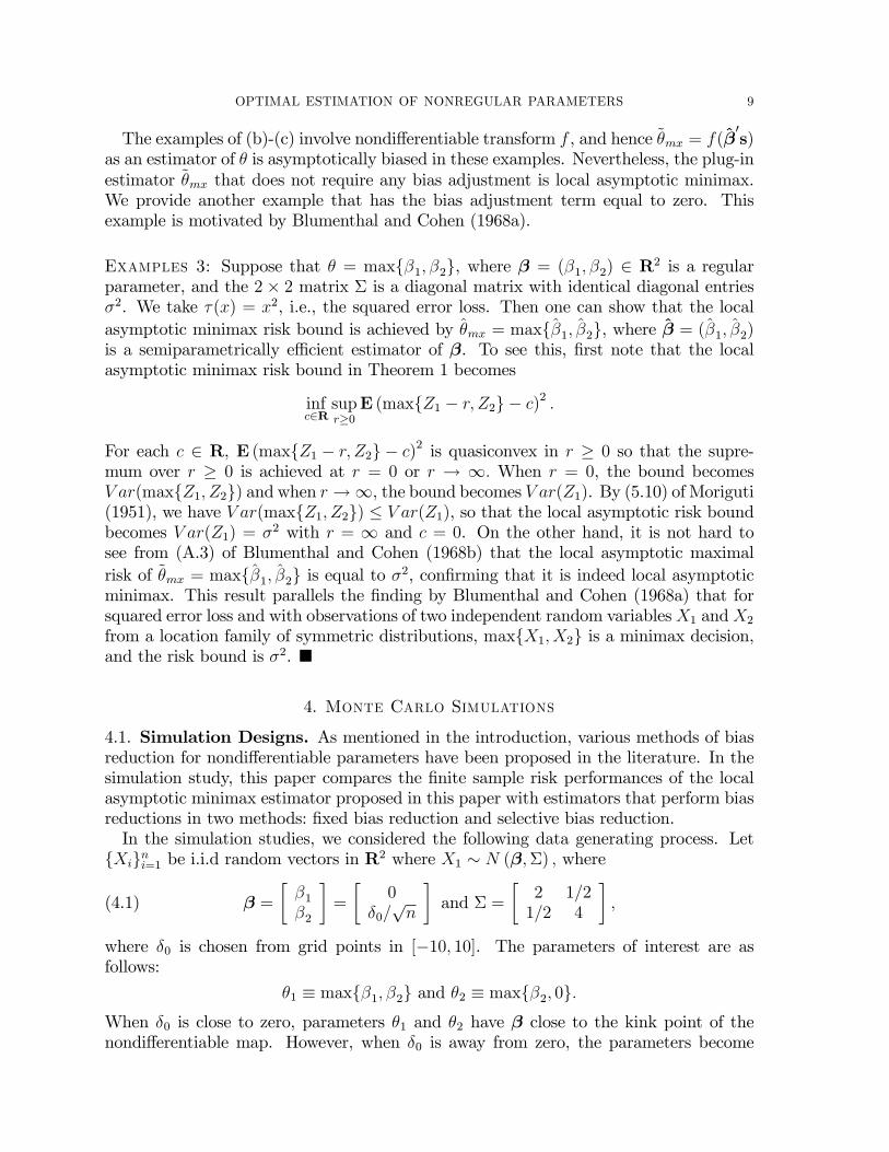
Figure 1. Comparison of the Local Asymptotic Minimax Estimatorswith Estimators Obtained through Other Bias-Reduction Methods: �1 =maxf�1; �2g.

more like a regular parameter themselves. We take � = 1n

Pni=1Xi as the estimator of

�. As for the �nite sample risk, we adopt the mean squared error:

Eh(�j � �j)2

i; j = 1; 2;

where �j is a candidate estimator for �j. We evaluated the risk using Monte Carlosimulations. The sample size was 300. The Monte Carlo simulation number was setto be 20,000. In the simulation study, we investigate the �nite sample risk pro�le ofdecisions by varying �0.

4.2. Minimax Decision and Bias Reduction for maxf�1; �2g. In the case of �1 �maxf�1; �2g, bF � E [maxfX11 � �1; X12 � �2g] becomes the asymptotic bias of theestimator �1 � maxf�1; �2g when �1 = �2. One may consider the following estimatorof bF :

bF �1

L

LXi=1

max��1=2�i

�,

where �i is drawn i.i.d. from N(0; I2). This adjustment term bF is �xed over di¤erentvalues of �2 � �1 (in large samples). Since the bias of maxf�1; �2g becomes prominentonly when �1 is close to �2, one may instead consider performing bias adjustment only


when the estimated di¤erence j�2 � �1j is close to zero. Thus we also consider thefollowing estimated adjustment term:

bS � 1

L

LXi=1

max��1=2�i

�!1nj�2 � �1j < 1:7=n1=3

o:

We compare the following two estimators with the minimax decision ~�mx:

�F � maxf�1; �2g � bF=pn and �S � maxf�1; �2g � bS=

pn:

We call �F the estimator with �xed bias-reduction and �S the estimator with selectivebias-reduction. The results are reported in Figure 1.The �nite sample risks of �F are better than the minimax decision �mx only locally

around �0 = 0. The bias reduction using bF improves the estimator�s performance inthis case. However, for other values of �0, the bias reduction does more harm than goodbecause it lowers the bias when it is better not to. This is seen in the right-hand panel ofFigure 1 which presents the �nite sample bias of the estimators. With �0 close to zero,the estimator with �xed bias-reduction eliminates the bias almost entirely. However,for other values of �0, this bias correction induces negative bias, deteriorating the riskperformances.The estimator �S with selective bias-reduction is designed to be hybrid between the

two extremes of �F and ~�mx: When �2 � �1 is estimated to be close to zero, the estima-tor performs like �F and when it is away from zero, it performs like maxf�1; �2g. Asexpected, the bias of the estimator �S is better than that of �F while successfully elimi-nating nearly the entire bias when �0 is close to zero. Nevertheless, it is remarkable thatthe estimator shows highly unstable �nite sample risk properties overall as shown on theleft panel in Figure 1. When �0 is away from zero and around 3 to 7, the performanceis worse than the other estimators. This result illuminates the fact that a reduction ofbias does not always imply a better risk performance.The minimax decision shows �nite sample risks that are robust over the values of

�0. In fact, the estimated bias adjustment term cM1 of the minimax decision is zero.This means that the estimator �mx requires zero bias adjustment, due to the concernfor its robust performance. In terms of �nite sample bias, the minimax estimator su¤ersfrom a substantially positive bias as compared to the other two estimators, when �0is close to zero. The minimax decision tolerates this bias because by doing so, it canmaintain robust performance for other cases where bias reduction is not needed. Theminimax estimator is ultimately concerned with the overall risk properties, not justa bias component of the estimator, and as the left-hand panel of Figure 1 shows, itperforms better than the other two estimators except when �0 is locally around zero, orwhen �2 � �1 is around roughly between �0:057 and 0:041.

4.3. Minimax Decision and Bias Reduction for maxf0; �2g. We consider �2 �maxf�2; 0g. The bias of the plug-in estimator �2 � maxf0; �2g; due to its asymmetricnature, might cause a concern at �rst glance. The bias at the kink point �2 = 0 is equal

12 K. SONG

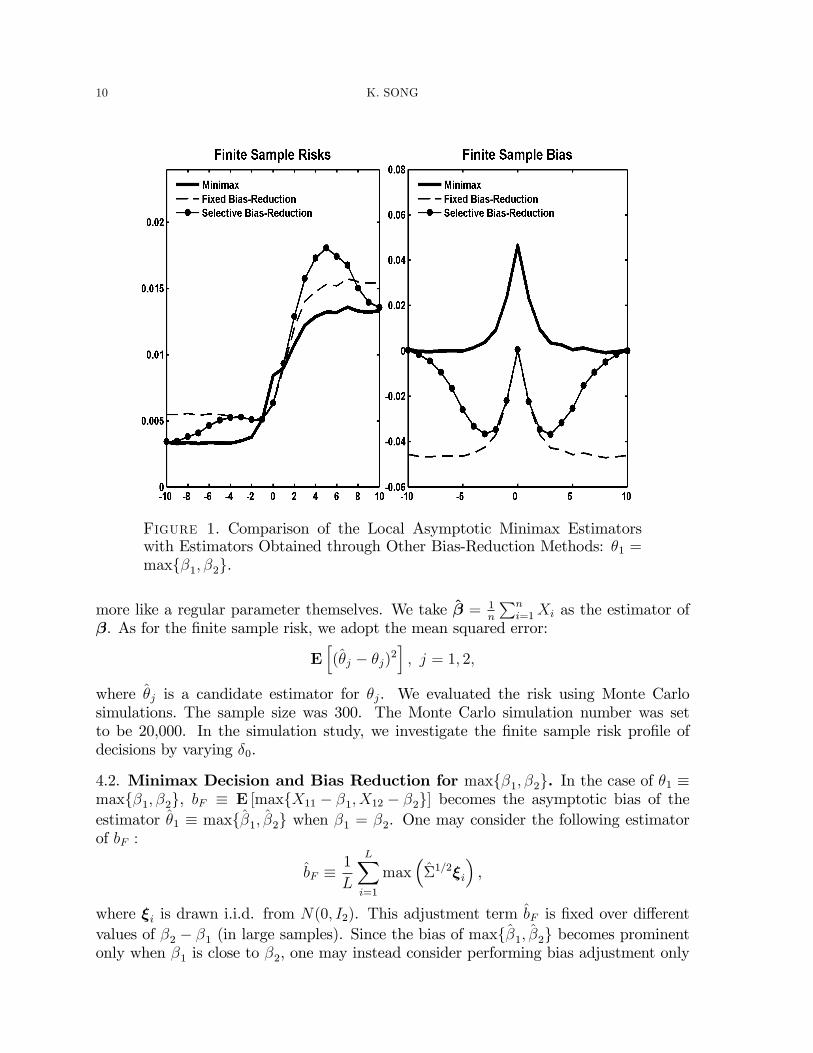
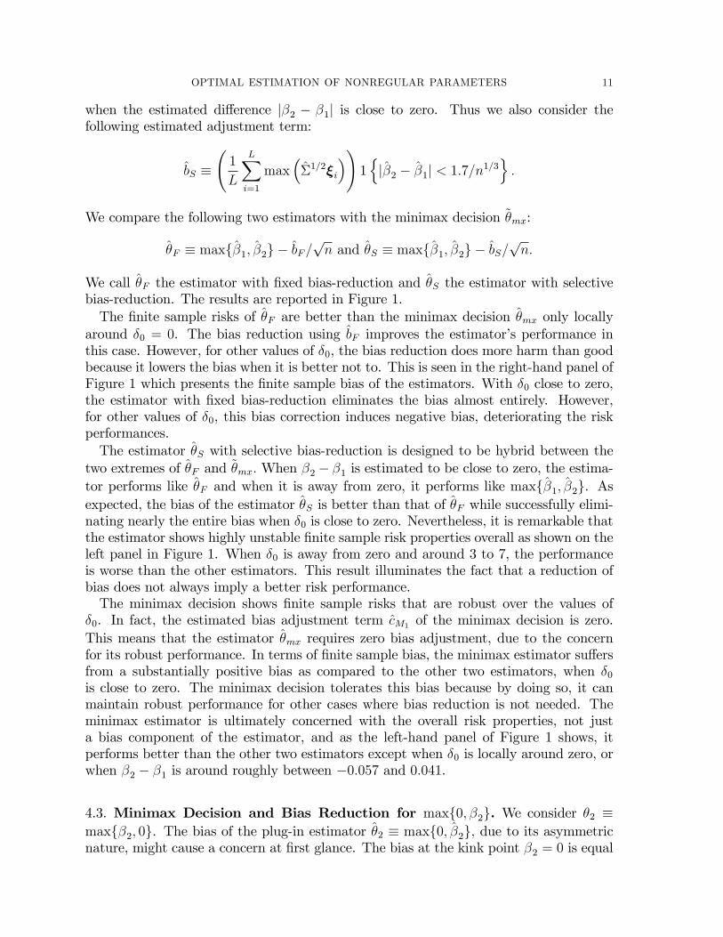
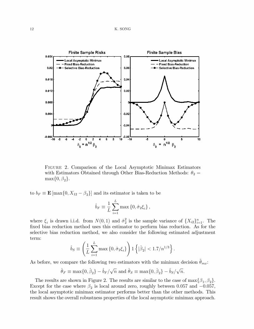
Figure 2. Comparison of the Local Asymptotic Minimax Estimatorswith Estimators Obtained through Other Bias-Reduction Methods: �2 =maxf0; �2g.

to bF � E [maxf0; X12 � �2g] and its estimator is taken to be

bF �1

L

LXi=1

max f0; �2�ig ,

where �i is drawn i.i.d. from N(0; 1) and �22 is the sample variance of fXi2gni=1. The�xed bias reduction method uses this estimator to perform bias reduction. As for theselective bias reduction method, we also consider the following estimated adjustmentterm:

bS � 1

L

LXi=1

max f0; �2�ig!1nj�2j < 1:7=n1=3

o:

As before, we compare the following two estimators with the minimax decision ~�mx:

�F � maxf0; �2g � bF=pn and �S � maxf0; �2g � bS=

pn:

The results are shown in Figure 2. The results are similar to the case of maxf�1; �2g.Except for the case where �2 is local around zero, roughly between 0:057 and �0:057,the local asymptotic minimax estimator performs better than the other methods. Thisresult shows the overall robustness properties of the local asymptotic minimax approach.


5. Conclusion

The paper proposes local asymptotic minimax estimators for a class of nonregularparameters that are constructed by applying translation-scale equivariant transform toa regular parameter. The results are extended to the case where the nonregular para-meters are transformed further by a piecewise linear map with a single kink. The localasymptotic minimax estimators take the form of a plug-in estimator with an additive biasadjustment term. The bias adjustment term can be computed by a simulation method.A small scale Monte Carlo simulation study demonstrates the robust �nite sample riskproperties of the local asymptotic minimax estimators, as compared to estimators basedon alternative bias correction methods.

6. Appendix: Mathematical Proofs

Proof of Lemma 1: First, suppose to the contrary that f1(y) 6= f2(y) for some y 2 R.Then since f1 � g1 = f2 � g2, it is necessary that g1(�) 6= g2(�) for some � 2 Rd suchthat g1(�) = y: Hence

(6.1) (f1 � g1)(�) 6= (f2 � g1)(�):

Now observe that f2(g1(�)) = f2(g2(�) + g1(�) � g2(�)) = f2(g2(� + g1(�) � g2(�))).Since f1 � g1 = f2 � g2, the last term is equal to

f1(g1(� + g1(�)� g2(�))) = f1(2g1(�)� g2(�)) = f1(g1(2� � g2(�)))= f2(g2(2� � g2(�))) = f2(g2(�)) = f1(g1(�)):

Therefore, we conclude that f2(g1(�)) = f1(g1(�)) contradicting (6.1).Second, suppose to the contrary that g1(�) 6= g2(�) for some � 2 Rd and f1 = f2.

First suppose that g1(�) > g2(�). Fix arbitrary a 2 R and c � 0 and let c� = c=�1;2(�)and �1;2(�) = g1(�)� g2(�). Then

f1(a+ c) = f1(a+�1;2(c��)) = f1(a+ g2(c��) + �1;2(c��)� g2(c��))= f1(g2(a+ c�� +�1;2(c��)� g2(c��)))= f2(g2(a+ c�� +�1;2(c��)� g2(c��)))= f1(g1(a+ c�� +�1;2(c��)� g2(c��)))= f1(a+ g1(c�� g2(c��) + c��1;2(�))) = f1(a+ 2c):

The choice of a 2 R and c � 0 are arbitrary, and hence f1(�) is constant on R, contra-dicting the nonconstancy condition for f1.Second, suppose that g1(�) < g2(�). Then, �x arbitrary a 2 R and c � 0 and let

c� = c=�1;2(�). Then similarly as before, we have

f1(a+ c) = f1(a+�1;2(c��))

= f1(a+ g1(c�� g2(c��) + c��1;2(�))) = f1(a+ 2c);

because �1;2(c��) = c. Therefore, again, f1(�) is constant on R, contradicting thenonconstancy condition for f1. �

14 K. SONG

We view convergence in distribution D! in the proofs as convergence in �Rd, so that thelimit distribution is allowed to be de�cient in general. Choose fhigmi=1 from an orthonor-mal basis fhig1i=1 of H. For p 2 Rm, we consider h(p) � �mi=1pihi so that _�j(h(p)) =Pm

i=1_�j(hi)pi; where _�j is the j-th element of _�: Let B be m� d matrix such that

(6.2) B �

26664_�1(h1)

_�2(h1) � � � _�d(h1)_�1(h2) _�2(h2) � � � _�d(h2)...

......

_�1(hm) _�2(hm) � � � _�d(hm)

37775 :We assume that m � d and B is a full column rank matrix. We also de�ne � �(�(h1); � � �; �(hm))0, where � is the Gaussian process that appears in Assumption 3, andwith � > 0, let F�;m(�) be the cdf of N(0; Im=�), and let Z�;m 2 Rd be a random vectorfollowing N(0;B0B=(�+ 1)).Let g : �Rd ! �R be a translation equivariant map, i.e., a map that satis�es Assump-

tions 1(i)(a) and (b). Suppose that � 2 R is a sequence of estimators such that alongfPn;0g; � p

nf� � g(�n(h))glog dPn;h=dPn;0

�D!�V � g( _�(h) + �g)�(h)� 1

2hh; hi

�;

for some nonstochastic vector �g 2 �Rd such that g(�g) whenever �g 2 Rd, and V 2 �Rd

is a random vector having a potentially de�cient distribution. Let Lhg be the limitingdistribution of

pnf� � g (�n(h))g in �Rd along fPn;hg for each h 2 H. The following

lemma is an adaptation of the generalized convolution theorem in van der Vaart (1989).

Lemma A1: Suppose that Assumptions 1(i) and 2-4 hold. For any � > 0; the distri-bution

RLh(p)g dF�(p) is equal to that of �g(Z�;m +W�;m + �g); where W�;m 2 �R is a

random variable having a potentially de�cient distribution independent of Z�;m.

Proof: Using Assumption 1(i) and applying Le Cam�s third lemma, we �nd that forall C 2 B(�R); the Borel �-�eld of �R,

Lh(p)g (C) =

ZEh1C(v � g(B0p+ �g))ep

0�� 12jjpjj2

idL0g(v)

=

ZEh1(�g)�1(C)(�v +B0p+ �g)ep

0�� 12jjpjj2

idL0g(v);

where (�g)�1(C) � fx 2 �Rd : �g(x) 2 Cg. The second equality uses translationequivariance of g. Let N� be the distribution of N(0; Im=(�+ 1)). We can writeZ

Lh(p)g (C)dF�;m(p)

=

ZEh1(�g)�1(C)

��v +B0p+ �g

�ep

0��+12jjpjj2

i� �2�

�m=2dL0g(v)dp

=

ZE

�1(�g)�1(C)

��v +B0

�p+

�

1 + �

�+ �g

�c�(�)

�dL0g(v)dN�(p);


where c�(�) � e1

2(�+1)�0� �(�=(�+ 1))m=2 :When we letW�;m be a random variable having

the distribution W�;m de�ned by

W�;m(C) �ZE

�1(�g)�1(C)

�v � B0�

1 + �

�c�(�)

�dL0g(v); C 2 B(�R);

the distributionRLh(p)g dF�(p) is equal to that of �g(Z�;m +W�;m + �g). �

We introduce some notation. De�ne jj�jjBL on the space of Borel measurable functionson Rd :

jjf jjBL � supx6=y

jf(x)� f(y)j=jjx� yjj+ supxjf(x)j:

For any two probability measures P and Q on B(Rd); de�ne

(6.3) dP(P;Q) � sup��Z fdP �

ZfdQ

�� : jjf jjBL � 1� :For the proof of Theorem 1, we employ two lemmas. The �rst lemma is Lemma 3 ofChamberlain (1987), which is used to write the risk using a distribution that has a �niteset support, and the second lemma is Theorem 3.2 of Dvoretsky, Wald, and Wolfowitz(1951).

Lemma A2 (Chamberlain (1987)): Let h : Rm ! Rd be a Borel measurable functionand let P be a probability measure on (Rm;B(Rm)) with a support AP � Rm. IfRjjhjjdP <1, then there exists a probability measure Q whose support is a �nite subset

of AP and ZhdP =

ZhdQ:

Lemma A3 (Dvoretsky, Wald and Wolfowitz (1951)): Let P be a �nite set ofdistributions on (Rm;B(Rm)), where each distribution is atomless, and for each P 2 P,let WP : R

m � T ! [0;M ] be a bounded measurable map with some M > 0, whereT � fd1; � � �; dJg is a �nite subset of R.Then, for each randomized decision � : Rm ! �T , with �T denoting the simplex on

RJ , there exists a measurable map v : Rm ! T such that for each P 2 P,JXj=1

ZRm

WP (x; dj)�j(x)dP (x) =

ZRm

WP (x; v(x))dP (x);

where �j(x) denotes the j-th entry of �(x).

Proof of Lemma 2: We writepnf� � g(�n(h))g

=pnf� � g(�n(0))g � g(

pn(�n(h)� �n(0)) + �n;g);

16 K. SONG

where �n;g =pnf�n(0) � g(�n(0))g. Applying Prohorov�s Theorem and invoking As-

sumption 2, we note that for any subsequence of fPn;0g, there exists a further subse-quence along which �n0;g ! �g, and� p

nf� � g(�n0(h))glog dPn0;h=dPn0;0

�D!�V � g( _�(h) + �g)�(h)� 1

2hh; hi

�;

where V 2 �Rd has a potentially de�cient distribution and �g is a nonstochastic vector in�Rd. From now on, it su¢ ces to focus only on these subsequences. Since g(�n;g) = 0 forall n � 1 by de�nition and by Assumption 1(i), we have g(�g) = 0, whenever �g 2 Rd.As in the proof of Theorem 3.11.5 of van der Vaart and Wellner (1996), choose an

orthonormal basis fhig1i=1 from �H. We �x m and take fhigmi=1 � H and considerh(p) =

Ppihi for some p = (pi)

mi=1 2 Rm such that h(p) 2 H: Fix � > 0 and let

F�;m(p) be as de�ned prior to Lemma A1. Hence note that for �xed M > 0;

liminfn!1

Rn(�) = liminfn!1

suph2H

Eh [�M (jVn;hj)]

� liminfn!1

ZEh(p)

��M��Vn;h(p)�� dF�;m(p);

where Vn;h �pnf��g(�n(h))g. By Lemma A1, the last liminf is equal toE[�M(jg(Z�;m+

W�;m + �g)j)], where Z�;m is as de�ned prior to Lemma A1 and W�;m 2 �R is a randomvariable having a potentially de�cient distribution and independent of Z�;m. It is nothard to see that for any sequence �m ! 0 as m ! 1, Z�m;m converges in distributionto Z. Since f[Z 0�;m;W�;m]

0 : (�;m) 2 (0;1)� f1; 2; � � �gg is uniformly tight in �Rd+1, byProhorov�s Theorem, for any subsequence of f�mg1m=1, there exists a further subsequencesuch that [Z 0�m;m;W�m;m]

0 converges in distribution to [Z 0;W ]0 for some random variableW having a potentially de�cient distribution. Since g(�g) = 0 whenever �g 2 Rd, webound liminfn!1Rn(�) from below by

supr2Rd:g(r)=0

E [�M (jg(Z +W + r)j)] = supr2Rd

E [�M (jg(Z +W + r� g(r))j)]

= supr2Rd

ZE [�M (jg(Z + r)� g(r) + wj)] dF (w);

where F is the (potentially de�cient) distribution of W . The �rst equality above followsbecause fr 2 Rd : g(r) = 0g = fr� g(r) : r 2 Rdg by the translation equivariance of g.Thus we conclude that

(6.4) liminfn!1

Rn(�) � limM"1

infF2F�

supr2Rd

ZE [�M(jg(Z + r)� g(r) + wj)] dF (w);

where F� is the collection of potentially de�cient distributions on B(R).Fix F 2 F� and let W 2 �R have distribution F . Suppose that PfW 2 �RnRg > 0.

For all r 2 Rd;

E [�M (jg(Z +W + r� g(r))j)] � E��M (jg(Z +W + r� g(r))j) 1fW 2 �RnRg

�:


For all u 2 �RnR, Z +u+ r� g(r) 2 �RnR, because Z + r� g(r) 2 R. Since u is a scalarand Z + r� g(r) 2 R, we have by Assumption 1(i)(a),

g(Z + u+ r� g(r)) = g(Z + r� g(r)) + u 2 f�1;1g, almost everywhere.

Hence for u 2 �RnR; �M (jg(Z + u+ r� g(r))j) =M; a.e., so that

E��M (jg(Z +W + r� g(r))j) 1fW 2 �RnRg

�= M � PfW 2 �RnRg " 1;

as M " 1. Therefore, the lower bound in (6.4) remains the same if we replace F� byF . Since �M increases in M , we obtain the desired bound by sending M " 1. �

Proof of Theorem 1: In view of Lemma 1, it su¢ ces to show that for each M > 0;

infF2F

supr2Rd

ZE [�M(jg(Z + r)� g(r) + wj)] dF (w)(6.5)

� infc2R

supr2Rd

E [�M(jg(Z + r)� g(r) + cj)] ;

because F includes point masses at points in R. The proof is complete then by sendingM " 1, because the last in�mum is increasing in M > 0. Let W 2 R be a randomvariable having distribution FW 2 F , and choose arbitrary M1 > 0 which may dependon the choice of FW 2 F ,

supr2[�M1;M1]d

E [�M (jg(Z +W + r� g(r))j) 1 fW 2 [�M1;M1]g](6.6)

� infu2R

supr2[�M1;M1]d

E [�M (jg(Z + u+ r� g(r))j)]PfW 2 [�M1;M1]g:

Once this inequality is established, we sendM1 " 1 on both sides to obtain the followinginequality:

supr2Rd

E [�M (jg(Z +W + r� g(r))j)]

� infu2R

supr2Rd

E [�M (jg(Z + u+ r� g(r))j)] :

(Note that by the de�nition of F , the distribution of W is tight in R.) And since thelower bound does not depend on the choice of FW , we take in�mum over FW 2 F of theleft hand side of the above inequality to deduce (6.5).We �x large enough M1 > 0 so that PfW 2 [�M1;M1]g > 0. Then

supr2[�M1;M1]d

E [�M (jg(Z +W + r� g(r))j) 1 fW 2 [�M1;M1]g]

� PfW 2 [�M1;M1]g � supr2[�M1;M1]d

Z[�M1;M1]

��(u; r)dFM1(u)

where ��(u; r) � E [�(Z + u+ r� g(r))] and �(x) � �M(jg(x)j); andZA\[�M1;M1]

dFM1(u) =

ZA\[�M1;M1]

dFW (u)=PfW 2 [�M1;M1]g;

18 K. SONG

for all A 2 B(R). Take K > 0 and let RK � fr1; � � �; rKg � [�M1;M1]d be a �nite

set such that RK become dense in [�M1;M1]d as K ! 1: Since

R��(u; r)dFM1(u) is

Lipschitz in r (due to Assumption 5), for any �xed � > 0, we can take RK such that

(6.7) maxr2RK

Z��(u; r)dFM1(u) � sup

r2[�M1;M1]d

Z��(u; r)dFM1(u)� �

Let FM1 be the collection of probabilities with support con�ned to [�M1;M1], so thatwe deduce that

supr2[�M1;M1]d

E [�M (jg(Z +W + r� g(r))j) 1 fW 2 [�M1;M1]g](6.8)

� PfW 2 [�M1;M1]g�inf

F2FM1

maxr2RK

Z[�M1;M1]

��(u; r)dF (u)� ��:

Since FM1 is uniformly tight, FM1 is totally bounded for dP de�ned in (6.3) (e.g. Theo-rems 11.5.4 of Dudley (2002)). Hence we �x " > 0 and choose F1; � � �; FN such that forany F 2 FM1 , there exists j 2 f1; � � �; Ng such that dP(Fj; F ) < ". Hence for F 2 FM1 ;we take Fj such that dP(Fj; F ) < ", so that��maxr2RK

Z��(u; r)dF (u)� max

r2RK

Z��(u; r)dFj(u)

�� maxr2RK

jj��(�; r)jjBL":

Since ��(�; r) is Lipschitz continuous and bounded on [�M1;M1], CK � maxr2RKjj��(�; r)jjBL <

1. Therefore,

(6.9) infF2FM1

maxr2RK

Z��(u; r)dF (u) � min

1�j�Nmaxr2RK

Z��(u; r)dFj(u)� CK":

By Lemma A2, we can select for each Fj and for each rk 2 RK a distribution Gj;k witha �nite set support such that

(6.10)Z��(u; rk)dFj(u) =

Z��(u; rk)dGj;k(u):

Then let TK;N be the union of the supports of Gj;k, j = 1; � � �; N and k = 1; � � �; K. Theset TK;N is �nite. Let FK;N be the space of discrete probability measures with a supportin TK;N . Then,

min1�j�N

max1�k�K

Z��(u; rk)dGj;k(u) � inf

G2FK;Nmaxr2RK

Z��(u; r)dG(u)

= infG2FK;N

maxr2RK

Z Z�(z + u)d�r(z)dG(u);

where �r is the distribution of Z + r� g(r).For the last infG2FK;N maxr2RK

, we regard Z + r� g(r) as a state variable distributedby �r with �r parametrized by r in a �nite setRK . We view the conditional distributionofW given Z+r�g(r) (which is G 2 FK;N) as a randomized decision. Each randomizeddecision has a �nite set support contained in TK;N ; and for each r 2 RK , �r is atomless.Finally � is bounded. We apply Lemma A3 to �nd that the last infG2FK;N maxr2RK

is equal to that with randomized decisions replaced by nonrandomized decisions (the


collection P and the �nite set fd1; � � �; dJg in the lemma correspond to f�r : r 2 RKgand TK;N respectively here), whereby we can now write it as

minu2TK;N

maxr2RK

Z�(z + u)d�r(z) = min

u2TK;Nmaxr2RK

E [�M(jg(Z + u+ r)� g(r)j)] :

Since E [�M(jg(Z + u+ r)� g(r)j)] is Lipschitz continuous in u and r, we send " # 0 andthen � # 0 (along with K " 1) to conclude from (6.7), (6.9), and (6.10) that

infF2FM1

supr2[�M1;M1]d

ZE [�(Z + u+ r� g(r))] dF (u)

� infu2R

supr2[�M1;M1]d

E [�M(jg(Z + r)� g(r) + uj)] :

Therefore, combining this with (6.8), we obtain (6.6). �

For given M1; a > 0 and c 2 R, de�ne(6.11) BM1(c; a) � sup

r2[�M1;M1]dE [�M1(ajg(Z + r)� g(r) + cj)] ;

and

EM1(a) ��c 2 [�M1;M1] : BM1(c; a) � inf

c12[�M1;M1]BM1(c1; a)

�:

Let c�M1(a) � 0:5 fsupEM1(a) + inf EM1(a)g. We simply write EM1 = EM1(1), BM1(c) =

BM1(c; 1), and c�M1= c�M1

(1).

Lemma A4: Suppose that Assumptions 1-2 hold.(i) There exists M0 > 0 such that for all M1 > M0 and for all a > 0;

c�M1= c�M1

(a):

(ii) There exists M0 such that for any M1 > M0 and " > 0;

suph2H

Pn;h��cM1 � c�M1

�� > "! 0;

as n; L!1 jointly.

Proof: (i) De�ne B(c; a) to be BM1(c; a) with M1 = 1: For any a > 0, we haveB(c; a) " 1, as jcj " 1. Therefore, the set(6.12) S � argminc2RB(c; a)is bounded in R. Note that the set S does not depend on a because � is a strictlyincreasing function. Increase M1 large enough so that S � [�M1;M1]. Then certainlyfor any a > 0;

c�M1(a) =

1

2fsupS + inf Sg ;

delivering the desired result.

(ii) Let S be the bounded set de�ned in (6.12). Take large M1 such that for some �" > 0;S � [M1+�";M1� �"]. Let the Hausdor¤ distance between the two subsets E1 and E2 ofR be denoted by dH(E1; E2). First we show that

(6.13) dH(EM1 ; EM1)!P 0;

20 K. SONG

as n ! 1 and L ! 1 uniformly over h 2 H. For this, we use arguments in theproof of Theorem 3.1 of Chernozhukov, Hong and Tamer (2007). Fix " 2 (0; �") and letE"M1

� fx 2 [�M1;M1] : supy2EM1jx � yj � "g. It su¢ ces for (6.13) to show that for

any " > 0;

(a) infh2H Pn;hnsupc2EM1

BM1(c) � infc2[�M1;M1]BM1(c) + �n;L

o! 1;

(b) infh2H Pn;hnsupc2EM1

BM1(c) < infc2[�M1;M1]nE"M1BM1(c)

o! 1,

as n; L ! 1 jointly, where the last term oP (1) is uniform over h 2 H. This is be-cause (a) implies infh2H Pn;hfEM1 � EM1g ! 1 and (b) implies that infh2H Pn;hfEM1 \([�M1;M1]nE"M1

) = ?g ! 1 so that infh2H Pn;hfEM1 � E"M1g ! 1; and hence for any

" > 0,

suph2HPn;hndH(EM1 ; EM1) > "

o! 0; as n; L!1 jointly.

We focus on (a). First, de�ne f(�; c; r) � �M1 (jg(� + r)� g(r) + cj) and J � ff(�; c; r) :(c; r) 2 [�M1;M1] � [�M1;M1]

dg. The class J is uniformly bounded, and f(�; c; r) isLipschitz continuous in (c; r) 2 [�M1;M1]� [�M1;M1]

d. Using the maximal inequality(e.g. Theorems 2.14.2 and 2.7.11 of van der Vaart and Wellner (1996)) and Assumptions1, 2, and 6(i), we �nd that for some CM1 > 0 that depends only on M1 > 0;

(6.14) E

"sup

c2[�M1;M1]

��BM1(c)�BM1(c)��# � CM1

�L�1=2 + n�1=2

:

The last bound does not depend on h 2 H. From this (a) follows because �n;Lpn!1

as n!1 and �n;LpL!1 as L!1.

Now let us turn to (b). Fix " > 0. By (6.14), with probability approaching 1 uniformlyover h 2 H;

supc2EM1BM1(c) � supc2EM1

BM1(c) + oP (1) � supc2E"=2M1

BM1(c) + oP (1)

� supc2E"=2M1

BM1(c) + oP (1);

where the second inequality follows due to �n;L ! 0 as n; L ! 1 and (6.14). Since�(�) is strictly increasing, and Z has full support on R by Assumption 4, we haveinfc2[�M1;M1]nE"M1

BM1(c) >supc2EM1BM1(c) � 0. Note that this last supremum does not

depend on h 2 H. Hence we obtain (b).For the main conclusion of the lemma, observe that

��cM1 � c�M1

�� is equal to1

2

��sup EM1 + inf EM1 � supEM1 � inf EM1

��which we can write as

1

2

�� infy2EM1

fy � supEM1g � supx2EM1

nx� inf EM1

o��=

1

2

�� supy2EM1

inf(y � EM1)� infx2EM1

supnx� EM1

o�� :


We write the last term as

1

2

�� supy2EM1

inf(y � EM1) + supx2EM1

infnEM1 � x

o�� 1

2

(supy2EM1

d(y; EM1) + supx2EM1

d(EM1 ; x)

);

where d(y; A) = infx2A jy�xj. The last term is bounded by dH(EM1 ; EM1). The desiredresult follows from (6.13). �

Proof of Theorem 2: Fix M > 0 and " > 0, and take M1 �M2 > M such that

supr2[�M2;M2]d

E��M(jg(Z + r)� g(r) + c�M1

j)�

(6.15)

� supr2Rd

E��M(jg(Z + r)� g(r) + c�M1

j)�� ":

This is possible for any choice of " > 0 because �M(�) is continuous and bounded by M .Note that

suph2H

Eh

h�M(

pnj� � �n(h)j)

i= sup

h2HEh

h�M(

pnjg(�) + cM1=

pn� g(�n(h))j)

i� sup

r2Rd

Eh

h�M(jg(

pnf� � �n(h)g+ r)� g(r) + cM1j)

i:

Using Lemma A4(ii) and Assumption 6, we observe that for all t 2 Rd;

Pn;hfpnf� � �n(h)g+ r� g(r) + cM1 � tg = P

�Z + r� g(r) + c�M1

� t+ o(1);

uniformly over h 2 H. Since Z is a continuous random vector, the convergence is uniformover (r; t) 2 Rd �R. Therefore,

limsupn!1

suph2H

Eh

h�M(


i= sup

r2Rd

E��M(jg(Z + r)� g(r) + c�M1

j)�

� supr2[�M2;M2]d

E��M(jg(Z + r)� g(r) + c�M1

j)�+ ";

by (6.15). Since M1 �M2 > M , the last supremum is bounded by

supr2[�M1;M1]d

E��M1(jg(Z + r)� g(r) + c�M1

j)�

= inf�M1�c�M1

supr2[�M1;M1]d

E [�M1(jg(Z + r)� g(r) + cj)] ;

where the equality follows by the de�nition of c�M1. We conclude that

limsupn!1

suph2H

Eh

h�M(


i� inf

�M1�c�M1

supr2Rd

E [�(jg(Z + r)� g(r) + cj)] + "

Since the choice of " and M1 were arbitrary, sending M1 " 1 and M2 " 1 (along with" # 0), and then sending M " 1, we obtain the desired result. �

22 K. SONG

Proof of Theorem 3: Suppose that f(x) has a kink point at x = m. Then write

f(g(�n(h))) = f(g(�n(h)�m) +m)� f(m) + f(m)= ~f(g(~�n(h)) + f(m);

where ~f(x) = f(x + m) � f(m) and ~�n(h) = �n(h) � m. Certainly ~�n(h) satis�esAssumption 3 for �n(h) and ~f satis�es Assumption 1(ii) for f , only with its kink pointnow at the origin. Therefore, we lose no generality by assuming that f has a kink pointat the origin, i.e.,

f(x) = a1x1 fx � 0g+ a2x1 fx < 0g ;for some constants a1 and a2 in R, and s = maxfja1j; ja2jg. Let

Hn;1(b) � fh 2 H : g(�n(h)) � bg; andHn;2(b) � fh 2 H : g(�n(h)) � bg:

First, note that

suph2H

Eh

h�(jpnf� � �n(h)gj)

i= sup

h2HEh

h�(jpnf� � f(g(�n(h)))gj)

i� max

k=1;2sup

h2Hn;k(0)Eh

h�M

�jpnf� � akg(�n(h))gj

�i:

Now we employ an argument similar to one in the proof of Theorem 3.1 of Blumenthaland Cohen (1968a). We �x arbitrary " > 0; and choose any large number b > 0. Notethat from su¢ ciently large n on,

suph2Hn;1(0)

Eh

h�M

�jpnf� � a1g(�n(h))gj

�i= sup

h2Hn;1(0)Eh

h�M

�jpnf� � a1b� a1g(�n(h)� b)gj

�i� sup

h2Hn;1(�b)Eh

h�M

�jpnf~� � a1g(�n(h))gj

�i� ";

where ~� � � � a1b. Let ~Vn;h �pnf~� � g(�n(h))g, h(p), p = (pi)mi=1 2 Rm, and F�;m(p)

be as in the proof of Lemma 2, so that we have

liminfn!1

suph2Hn;1(�b)

Eh

h�M

�jpnf~� � a1g(�n(h))j

�i� liminf

n!1

Zfp2Rm:h(p)2Hn;1(�b)g

Eh

h�M

�j ~Vn;h(p)j

�idF�;m(p):

Since �M is bounded by M , we take b large enough so that the last liminf is boundedfrom below by

liminfn!1

ZEh

h�M

�j ~Vn;h(p)j

�idF�;m(p)� ":

By following the same arguments as in the proofs of Lemma 2 and Theorem 1, we deducethat the last liminf is bounded from below by

infc2R

supr2Rd

E [�M(ja1jjg(Z + r)� g(r) + cj)]� ":


We proceed similarly with suph2Hn;2(0)Eh[�M(jpnf� � a2g(�n(h))gj)] to conclude that

liminfn!1

suph2H

Eh[�(jpnf� � �n(h)gj)]

� maxk=1;2

infc2R

supr2Rd

E [�M(jakjjg(Z + r)� g(r) + cj)]� 3"

= infc2R

supr2Rd

E [�M(sjg(Z + r)� g(r) + cj)]� 3";

where the last equality follows because �M is an increasing function. By sendingM " 1and " # 0, we obtain the desired result. �

Proof of Theorem 4: First, observe that a real valued map that assigns y 2 Rto f(y)=s is a contraction mapping, because the maximum absolute slope of the linesegments of f is equal to s. Hence for M > 0;

suph2H

Eh

h�M(j

pnf~�mx � �n(h)gj)

i� sup

h2HEh

h�M(s

pnjg(�) + cM1=

pn� g(�n(h))j)

i:

Fix " > 0, chooseM1 �M , and follow the proof of Theorem 2 to �nd that the limsupn!1of the last supremum is bounded by

supr2[�M1;M1]d

E��M1(sjg(Z + r)� g(r) + c�M1

j)�+ ":

By Lemma A4(i), from some large M1 on, the last supremum is equal to

supr2[�M1;M1]d

E��M1(sjg(Z + r)� g(r) + c�M1

(s)j)�

= infc2[�M1;M1]

supr2[�M1;M1]d

E��M1(sjg(Z + r)� g(r) + c�M1

(s)j)�

� infc2[�M1;M1]

supr2Rd

E [�(sjg(Z + r)� g(r) + cj)] :

Sending M1 " 1, we obtain the desired result. �

7. Acknowledgement

I thank Keisuke Hirano, Marcelo Moreira, Ulrich Müller and Frank Schorfheide forvaluable comments. This research was supported by the Social Sciences and HumanitiesResearch Council in Canada.

References

[1] Begun, J. M., W. J. Hall, W-M., Huang, and J. A. Wellner (1983): �Information andasymptotic e¢ ciency in parametric-nonparametric models,�Annals of Statistics, 11, 432-452.

[2] Bickel, P. J. (1981): �Minimax estimation of the mean of a normal distribution when the para-meter space is restricted,�Annals of Statistics, 9, 1301-1309.

[3] Bickel, P. J. , A.J. Klaassen, Y. Rikov, and J. A. Wellner (1993): E¢ cient and AdaptiveEstimation for Semiparametric Models, Springer Verlag, New York.

[4] Blumenthal, S. and A. Cohen (1968a): �Estimation of the larger translation parameter,�Annals of Mathematical Statistics, 39, 502-516.

24 K. SONG

[5] Blumenthal, S. and A. Cohen (1968b): �Estimation of the larger of two normal means,�Journal of the American Statistical Association, 63, 861-876.

[6] Boubarki, N. (1970): Theory of Sets, Springer-Verlag.[7] Casella G. and W. E. Strawderman (1981): �Estimating a bounded normal mean,�Annals

of Statistics, 9, 870-878.[8] Charras, A. and C. van Eeden (1991): �Bayes and admissibility properties of estimators in

truncated parameter spaces,�Canadian Journal of Statistics, 19, 121-134.[9] Chernozhukov, V., S. Lee and A. Rosen (2009): �Intersection bounds: estimation and infer-

ence,�Cemmap Working Paper, CWP 19/09.[10] Doss, H. and J. Sethuraman (1989): �The price of bias reduction when there is no unbiased

estimate,�Annals of Statistics, 17, 440-442.[11] Dudley, R. M. (2002): Real Analysis and Probability, Cambridge University Press, New York.[12] Dvoretsky, A., A. Wald. and J. Wolfowitz (1951): �Elimination of randomization in certain

statistical decision procedures and zero-sum two-person games,�Annals of Mathematical Statistics22, 1-21.

[13] Haile, P. A. and E. Tamer (2003): �Inference with an incomplete model of English auctions,�Journal of Political Economy, 111, 1-51.

[14] Hájek, J. (1972): �Local asymptotic minimax and admissibility in estimation,� in L. Le Cam,J. Neyman and E. L. Scott, eds, Proceedings of the Sixth Berkeley Symposium on MathematicalStatistics and Probability, Vol 1, University of California Press, Berkeley, p.175-194.

[15] Hirano, K. and J. Porter (2012): �Impossibility results for nondi¤erentiable functionals,�Forthcoming in Econometrica.

[16] Le Cam, L. (1979): �On a theorem of J. Hájek,� in J. Jureµcková, ed. Contributions to Statistics- Hájek Memorial Volume, Akademian, Prague, p.119-135.

[17] Lehmann E. L. (1986): Testing Statistical Hypotheses, 2nd Ed. Chapman&Hall, New York.[18] Lovell, M. C. and E. Prescott (1970): �Multiple regression with inequality constraints:

pretesting bias, hypothesis testing, and e¢ ciency,�Journal of the American Statistical Association,65, 913-915.

[19] Manski C. F. and J. Pepper (2000): �Monotone instrumental variables: with an application tothe returns to schooling,�Econometrica 68, 997�1010.

[20] Milgrom, P. J. and R. J. Weber (1985): �Distributional strategies for games with incompleteinformation,�Mathematics of Operations Research, 10, 619-632.

[21] Moors, J. J. A. (1981): �Inadmissibility of linearly invariant estimators in truncated parameterspaces,�Journal of the American Statistical Association, 76, 910-915.

[22] Moriguti, S. (1951): �Extremal properties of extreme value distribution,�Annals of MathematicalStatistics, 22, 523-536.

[23] Strasser, H. (1985): Mathematical Theory of Statistics, Walter de Gruyter, New York.[24] Takagi, Y. (1994): �Local asymptotic minimax risk bounds for asymmetric loss functions,�Annals

of Statistics 22, 39�48.[25] van der Vaart, A. W. (1989): �On the asymptotic information bound,�Annals of Statistics 17,

1487-1500.[26] van der Vaart, A. W. (1991): �On di¤erentiable functionals,�Annals of Statistics 19, 178-204.[27] van der Vaart, A. W. and J. A. Wellner (1996): Weak Convergence and Empirical Processes,

Springer-Verlag, New York.[28] van Eeden, C., and J. V. Zidek (2004): �Combining the data from two normal populations

to estimate the mean of one when their means di¤erence is bounded,� Journal of MultivariateAnalysis 88, 19-46.

Department of Economics, University of British Columbia, 997 - 1873 East Mall,Vancouver, BC, V6T 1Z1, CanadaE-mail address: [email protected]

local asymptotic minimax estimation of ......local asymptotic minimax estimation of nonregular...

Documents