Local Content Requirements and Industrial Development

Economic Analysis and Cost Modeling of the Automotive Supply Chain

by

Francisco Veloso

Licenciatura em Engenharia Física Tecnológica Instituto Superior Técnico, UTL, Lisboa, 1992

M.S. Economia e Gestão de Ciência e Tecnologia Instituto Superior de Economia e Gestão, UTL, Lisboa, 1996

Submitted to the Engineering Systems Division in Partial Fulfillment of the Requirements for the Degree of

Doctor of Philosophy in Technology, Management and Policy at the

Massachusetts Institute of Technology

February 2001

© 2001 Massachusetts Institute of Technology. All Rights Reserved

Signature of Author Technology, Management and Policy Program

Engineering Systems Division

Certified by Alice H. Amsden

Professor of Political Economy Thesis Supervisor

Certified by Joel P. Clark

Professor of Engineering Systems & Materials Engineering

Certified by Richard de Neufville

Professor of Engineering Systems & Civil and Environmental Engineering

Accepted by Daniel E. Hastings

Professor of Engineering Systems & Aeronautics and Astronautics Co-Director, Technology and Policy Program

- 2 -

Local Content Requirements and Industrial Development:

Economic Analysis and Cost Modeling of the Automotive Supply Chain

by Francisco Veloso

Submitted to the Engineering Systems Division on January 12, 2001 in Partial Fulfillment of the Requirements for the Degree of

Doctor of Philosophy in Technology, Management and Policy

ABSTRACT

This dissertation addresses the issue of performance standards in developing nations, focusing on the role of local content requirements. It proposes a theoretical framework to understand the impact of this policy on the decisions of firms and the welfare of the domestic economy, and offers a methodology to apply the analysis to the context of the automotive supply chain. The central conclusion of the thesis relates to the existence of a gap between private and social opportunity returns and costs, an aspect that has been overlooked by previous literature.

In a developing country, resources employed by foreign investors and their local suppliers often generate spillovers and learning effects that are not accounted for in the valuations of private economic agents. This creates an externality-from-entry, whereby positive economic effects of new domestic suppliers are overlooked in the sourcing decision of the foreign firm. This dissertation proposes a model to illustrate how this gap between social and private valuations justifies the enactment of domestic content requirements, which become welfare enhancing. The analysis also reveals that content requirements are a preferable policy to tariffs and subsidies as a means to increase domestic purchases and discusses the use of subsidies and requirements as incentive mechanisms to align firm decisions with government objectives.

A case study of the automotive industry, where content restriction policies are extremely active, is used to demonstrate the applicability of the model. This entailed the development of a new methodology, called Systems Cost Modeling (SCM), which uses simple metrics and rules to build bottom-up cost structures where estimates for large number of components have to be considered. Detailed empirical data from a particular car is then used to build a sourcing cost structure. These costs are integrated with the domestic content model to show how, for existing market and policy conditions; there can be value to the enactment of modest levels of domestic content requirements in the auto industry. It also explains that the impact of the policy is very sensitive to project characteristics and that this should be factored into national decisions.

Thesis Supervisor: Alice H. Amsden Title: Professor of Political Economy

- 3 -

ACKNOWLEDGMENTS

I would like to acknowledge the generous financial support of Praxis XXI and Fundação Calouste Gulbenkian for my MIT studies. I also wish to thank INTELI for travel support.

I would like to thank my advisors for their guidance, support and friendship throughout my tenure at the MIT. Professor Alice Amsden provided the initial stimulation for this thesis and has been since then an inexhaustible source of insightful and provocative thoughts, not only about my work, but also on how to think about industrial development. Professor Richard de Neufville has been a dedicated mentor since my first day here. His advice, encouragement and careful reflections have been instrumental in all the steps of my education and research at MIT. Professor Joel Clark deposited immense confidence in me. Not only he has accepted me in the Materials Systems Laboratory and provided financial and intellectual support, but he has also willingly taken a strong personal and institutional involvement in a set of projects that I suggested. My sincere thank you also goes to the unofficial member of the committee, Dr. Richard Roth. He has been an enthusiastic supporter of my work, providing significant insights to the dissertation, as well as detailed comments on grammar and structure. Through his guidance of the ‘Portugal’ project, I have learned a great deal a bout manufacturing, and I have come to value his friendship.

I also want to recognize the importance of MSL, where it has been a great pleasure to work. The warm advice of Dr. Frank Field and Dr. Randy Kirchain is invaluable and the interactions with all the other students provide a unique learning and human experience. Thank you Ashish, Alexandra, Bruce, Chris, Erika, Gilles, Luis, Mon, Patrick, and Randy for the wonderful time. Special thank you for my friend Sebastian, which has been my daily companion of long academic discussions, frequent working nights, regular squash and irregular drinking (to be corrected in the future). The same appreciation goes to my friends at TPP and TMP, in particular Enrique, Ian, Jason, Mag and Pato, with whom I have learned to appreciate life at MIT and around Cambridge.

The Portuguese ‘connection’ has also been an important ingredient during these years. Among many others, my good friends José Rui, Manuel Heitor and Pedro Conceição have been part of my work since well before entering MIT. Their strong encouragement, the intense collaboration and the common goals are a constant source of motivation. I am particularly indebted to José Rui, personally and through the INTELI team. He has always been a major stimulus and a partner in a number of endeavors (I know, more work is waiting for us!). My involvement in PSA and PAPS provided an escape from research and an opportunity to meet extraordinary persons that have been a supply of stimulation and many joyful events. Among many, I thank Pedro Ferreira for being a good friend and a cheerful companion (more cigars to come).

Finally I want to thank my family for their unwavering confidence and warm feelings despite the distance and the absence. Notwithstanding the physical separation, my spirit is particularly close to my mother and my youngest brother. David has shared with me some of the most difficult, as well as the most awesome periods of my existence, and our time together here in Cambridge has made him a true element of my life. Through her immense generosity, her devoted love for the family and an intense strength and will power, my mother has always been a foremost inspiration. This period at MIT was no exception. Thank you both so much. This work is for you. At heart, my thanks go to Inês, for her love, encouragement, patience, and bringing joy to my everyday life.

- 4 -

TABLE OF CONTENTS

CHAPTER 1. OVERVIEW........................................................................................................................................ 8

CHAPTER 2. FOREIGN INVESTMENT, SUPPLY CHAIN STRUCTURES AND DOMESTIC CONTENT REGULATION: A REVIEW OF THE ISSUES .................................................................................................... 17 2.1. Foreign Direct Investment and Supply Chain Decisions ......................................................................... 17 2.2. Development, Foreign Participation and the Role of Linkages .............................................................. 20 2.2.1. Foreign Investment, Externalities and the Gap Between Social and Private Returns ................................... 21 2.2.2. Linkages and Spillovers................................................................................................................................ 23 2.2.3. Foreign Investment and Imperfect Markets .................................................................................................. 26 2.2.4. Policy Considerations ................................................................................................................................... 26 2.3. Performance Standards as Catalysts of Local Economic Development ................................................. 27 2.4. Understanding the Impact of Domestic Content Requirements ............................................................. 31 2.4.1. Models of Performance Standards with a Focus on Local Content Requirements........................................ 31 2.4.2. Empirical Assessment of Local Content Policies and Decisions .................................................................. 35 2.4.3. WTO, TRIMS and he Use of Performance Standards .................................................................................. 39 2.5. Research Question, Hypothesis and Methodology................................................................................... 41

CHAPTER 3. A MODEL TO EVALUATE LOCAL CONTENT DECISIONS ................................................. 44 3.1. Valuing Investments in a Local Economy................................................................................................. 44 3.2. Domestic Content Policies and Private Sourcing Decisions .................................................................... 47 3.2.1. The Natural Sourcing Decision..................................................................................................................... 49 3.2.2. The Effect of Domestic Content Requirements............................................................................................. 54 3.3. Benchmarking Domestic Content Policies ................................................................................................ 56 3.3.1. Are Domestic Content Requirements Better Than Tariffs? .......................................................................... 57 3.3.2. Subsidies and Domestic Content Requirements............................................................................................ 61 3.4. Externalities and the Social Evaluation of Domestic Content................................................................. 63 3.4.1. Differences in Private and Social Opportunity Costs.................................................................................... 64 3.4.2. Learning and External Effects....................................................................................................................... 70 3.5. Model Extension: Cost Uncertainty and Risk Averse Managers ........................................................... 74 3.6. Summary...................................................................................................................................................... 77

CHAPTER 4. PERFORMANCE STANDARDS, INFORMATION AND CONTENT DECISIONS ............... 78 4.1. Content Requirements and Subsidies as Performance Standards.......................................................... 78 4.1.1. Understanding Performance Standards ......................................................................................................... 78 4.1.2. Using Performance Standards to Establish Incentive Contracts ................................................................... 81 4.2. The Formal Model ...................................................................................................................................... 84 4.2.1. Base Case: First Best .................................................................................................................................... 86 4.2.2. Asymmetric Information: Second Best ......................................................................................................... 88 4.2.3. Deviations From Optimal Behaviour ............................................................................................................ 91 4.3. Summary...................................................................................................................................................... 93

- 5 -

CHAPTER 5. SCM - SYSTEM COST MODELING ............................................................................................ 95 5.1. Manufacturing Cost Modeling .................................................................................................................. 96 5.2. Technical Cost Modeling............................................................................................................................ 99 5.2.1. Fixed Costs ................................................................................................................................................... 99 5.2.2. Variable Costs............................................................................................................................................. 104 5.2.3. The Process Time Use of Resources........................................................................................................... 105 5.2.4. Technical Cost Modeling Extensions.......................................................................................................... 108 5.3. Systems Cost Modeling (SCM): Estimating the manufacturing cost of complex systems .................. 111 2.4.1. Estimating Fixed Cost Drivers .................................................................................................................... 114 5.3.1. Variable Costs............................................................................................................................................. 121 5.3.2. Valuing the Process Use of Resources........................................................................................................ 123 5.3.3. Logistics Costs............................................................................................................................................ 125 5.4. Summary.................................................................................................................................................... 126

CHAPTER 6. MODELING COST IN THE AUTOMOTIVE SUPPLY CHAIN.............................................. 128 6.1. The Automotive Supply Chain................................................................................................................. 128 6.1.1. Global Trends in the Auto Industry ............................................................................................................ 128 6.1.2. Understanding OEM Purchasing Policies and Decisions............................................................................ 133 6.2. Modeling Automotive Supply Chain Costs............................................................................................. 137 6.2.1. Unbundling the Car Structure ..................................................................................................................... 138 6.2.2. The Cost of the Auto Supply Chain ............................................................................................................ 140 6.2.3. The impact of Regional Condition on Manufacturing Cost ........................................................................ 147 6.3. Summary.................................................................................................................................................... 152

CHAPTER 7. DOMESTIC CONTENT REQUIREMENTS AND THE AUTO SUPPLY CHAIN................. 153 7.1. Domestic Content Policies in the Auto Industry .................................................................................... 153 7.2. Estimating Welfare Effects of Domestic Content Policies ..................................................................... 156 7.2.1. Market Conditions and Sourcing Decisions................................................................................................ 157 7.2.2. The Social Opportunity Cost and the Welfare Effect of a Content Policy.................................................. 161 7.2.3. Sensitivity to Key Variables ....................................................................................................................... 163 7.2.4. Externalities and Learning Effects .............................................................................................................. 166 7.2.5. Risk Averse Decisions ................................................................................................................................ 172 7.3. Incentive Contracts, Asymmetric Information and Content Decisions................................................ 174 7.3.1. The Optimal Incentive Contract.................................................................................................................. 174 7.3.2. Degree of Uncertainty, Government Menus and Firm Decisions ............................................................... 176 7.4. Summary.................................................................................................................................................... 181

CHAPTER 8. CONCLUSIONS AND FUTURE WORK .................................................................................... 183 8.1. Conclusions................................................................................................................................................ 183 8.2. Future Work.............................................................................................................................................. 186

CHAPTER 9. APPENDIX...................................................................................................................................... 188 9.1. Appendix with Details of the Demonstrations of Chapter 4.................................................................. 188 9.1.1. Calculations for Asymmetric Information................................................................................................... 188 9.1.2. Deviations from Optimality ........................................................................................................................ 190 9.2. Information for SCM Calculations in Chapters 5 and 6 ....................................................................... 192

REFERENCES........................................................................................................................................................ 210

- 6 -

LIST OF FIGURES

Figure 3–1: Sourcing Options for the OEM................................................................................................................ 50 Figure 3–2: Ordering Components Through the Sourcing Index ................................................................................ 51 Figure 3–3: OEM Sourcing Cost as a Function of Component Sourcing Index........................................................ 52 Figure 3–4: Correspondence between Index and Domestic Content Level................................................................. 53 Figure 3–5: Effect of a Tariff on Purchasing Decisions .............................................................................................. 59 Figure 3–6: Effect of a subsidy on Purchasing Decisions ........................................................................................... 62 Figure 3–7: Example of Positive Surplus from Forced Localization .......................................................................... 67 Figure 3–8: Welfare Effects of Local Content Requirements .................................................................................... 69 Figure 4–1: A Framework to understand Performance Standards............................................................................... 80 Figure 5–1: Equipment Cost Estimation Techniques for Technical Cost Modeling ................................................. 100 Figure 5–2: Critical Relationships in Line Utilization .............................................................................................. 107 Figure 5–3: Estimating Component Manufacturing Cost Through SCM.................................................................. 112 Figure 5–4: Equipment Cost Estimation Process for SCM ....................................................................................... 115 Figure 5–5: Three Point Estimation of Equipment Cost ........................................................................................... 118 Figure 5–6: Three Point Estimation of Tool Cost ..................................................................................................... 120 Figure 5–7: Cycle Time Estimation for Stamping Example...................................................................................... 124 Figure 6–1: New Vehicle Sales in Triad Versus the Rest of the World .................................................................... 129 Figure 6–2: Typical Supplier Approval Process for VW .......................................................................................... 135 Figure 6–3: Price reductions demanded from Assemblers. ....................................................................................... 136 Figure 6–4: Car Manufacturing Cost......................................................................................................................... 144 Figure 6–5: Major Cost Drivers of the Car Supply Chain......................................................................................... 145 Figure 6–6: Sensitivity Analysis of Cost to Main Model Assumptions..................................................................... 146 Figure 6–7: Supply Chain Cost breakdown for Developing Area ............................................................................. 150 Figure 7–1: Car Supply Chain Costs (Unit Value).................................................................................................... 156 Figure 7–2: Component Sourcing Cost Tradeoffs..................................................................................................... 158 Figure 7–3: Welfare Effects of Content Requirements in Perfect Market................................................................. 159 Figure 7–4: Comparing Welfare effects of Local Content and Tariffs...................................................................... 160 Figure 7–5: Welfare Effects of a Domestic Content Policy ...................................................................................... 162 Figure 7–6: Sensitivity Analysis for Key Factors...................................................................................................... 164 Figure 7–7: The implications of Volume for Domestic Content ............................................................................... 165 Figure 7–8: Learning by Doing and Domestic Content............................................................................................. 168 Figure 7–9: Learning by Spillovers and Domestic Content....................................................................................... 169 Figure 7–10: Joint Learning and Domestic Content.................................................................................................. 170 Figure 7–11: The Impact of Risk Aversion in Domestic Sourcing............................................................................ 173 Figure 7–12: Incentive Contract to Drive Domestic Content .................................................................................... 175 Figure 7–13: Menu of Contracts Offered as a Function of Uncertainty .................................................................... 178 Figure 7–14: Welfare Gain and Uncertainty in Sourcing Cost.................................................................................. 180

- 7 -

LIST OF TABLES

Table 5–1: Generic Functional Relationship Between Weight, Equipment Key Characteristic and Cost................. 116 Table 5–2: Time Required for Joining Processes...................................................................................................... 122 Table 5–3: Handling Time for Components.............................................................................................................. 123 Table 6–1: Components and Sub-Assemblies by Group ........................................................................................... 139 Table 6–2: Assumptions Used in System Cost Model Estimations........................................................................... 140 Table 6–3: Examples of Sub-Assembly Cost - SCM Estimate and Data Provided by OEM .................................... 143 Table 6–4: Assumptions used in System Cost Model Estimations............................................................................ 148 Table 6–5: Examples Subassembly Cost on Developed and Developing Region ..................................................... 151 Table 7–1: Domestic Content Requirements in Selected Regions ............................................................................ 155 Table 9–1: Material Prices Used in Calculations ...................................................................................................... 192 Table 9–2 Base Inputs for Foreign Component SCM Estimation ............................................................................. 193 Table 9–3 Base Inputs for Domestic Component SCM Estimation .......................................................................... 193 Table 9–4: Key Parameters for Technologies Considered in the SCM Estimation Process...................................... 194 Table 9–5: Component List and Characteristics ....................................................................................................... 195

- 8 -

Chapter 1. Overview

This thesis addresses the question of performance standards in developing nations. In particular,

it aims at providing further understanding of the conditions under which local content

requirements (LCR) on foreign investors can have a positive welfare impact on the host

economy. Local content requirements is a policy enacted by governments that forces a firm or all

the companies in an industry to source a certain share of the inputs used in the manufacturing

process from the domestic market. It has been widely used throughout the world, principally in

the context of the developing world.

Local content requirements have been extensively discussed in the context of trade, foreign

investment and industrial development issues. International organizations, in particular the World

Trade Organization (WTO), have strongly attacked these policies, but policy makers in

developing countries continue to be firm believers in their potential benefits. In fact, while

content requirements may formally disappear at a national level in the future because of WTO

regulations on Trade Related Investment Measures, they are likely to continue on an informal

basis, at a supra-national basis and explicitly in developing countries, which have been given

some latitude in the adoption of these regulations. Meanwhile, multinationals actively pressure

against content policies, but have mostly chosen to abide and sometimes surpass these

requirements whenever present. This set of inconsistent perspectives and the limited research in

the subject generate the opportunity for the dissertation.

Theoretical models and empirical analysis seem to point to the existence of competing views on

the potential role of local content requirements. The small amount of empirical research on the

issue has documented evidence of both good and bad outcomes of this policy. Analysis shows

that the impact of the policy on companies and domestic welfare seems to depend on a number of

different aspects ranging from industry conditions to the degree of discretion in the policy or the

severity of the requirement. Nevertheless, most economic models proposed so far seem to

discourage these types of policies. They explain how, under most circumstances, domestic

content requirements increase the cost of intermediate goods and, consequentially, the price of

- 9 -

the final good, leading to higher prices and an inevitable reduction of consumer surplus.

Although consumer surplus is partially transferred to producers, some deadweight loss that

reduces country welfare is also generated. The problem is that most research has focused on rent-

shifting effects of these policies and has overlooked the potential role that external and learning

effects play in host countries, precisely the issues that have been the core motivation for the

enactment of these policies.

One question is why enacting local content requirements and not alternative policies such as

tariffs or subsidies to local producers? In fact, it is intuitive to understand that a tariff on

imported components will make domestic production of some of these components more

attractive. Local firms that could not previously compete on price suddenly become competitive,

and therefore it is likely that domestic content increases. This is precisely the initial aspect that

the dissertation covers. A simple model is proposed to compare domestic content requirements

with potential substitutes, aiming at understanding their merits and demerits.

The core of the dissertation, nevertheless, is a study of the potential role of local content as a

mechanism to correct a gap between private and social benefits arising from foreign investment

in a host nation. In a developing country, a new large OEM investment in an industry like

automotive generates a unique opportunity for a set of local firms to enter into the manufacturing

of complex products like automotive components. Because of spillovers or learning effects, this

possibility tends to propel the overall capability of the industry to levels that would not be

attainable by alternative means. Under some circumstances, these industry external effects are

not accounted in the valuations of private economic agents. This gap between private and social

valuations generates the opportunity for the enactment of domestic content requirements. The

dissertations develops a model to study how this policy can be welfare enhancing in the presence

of these extra social benefits.

This study also covers implementation. The question it addresses is how a government can lure

an investing OEM into compliance with a particular level of domestic content without creating

an obvious price distortion in the final good. This is an important aspect because it has been at

the core of the negative evaluation that previous authors have made on the subject. An incentive

model is used to assess this problem.

- 10 -

A case study for the automotive industry, where content restriction policies are extremely active,

is used to demonstrate the applicability of the theoretical models mentioned in the previous

paragraphs. To build the automotive sourcing cost structure required for the analysis, the

dissertation proposes a new methodology, called Systems Cost Modeling (SCM), which enables

bottom-up estimates of component manufacturing costs. Detailed empirical data from a typical

mid size car is then used to evaluate local content requirements according to the aspects outlined

above.

This thesis has contributions in three areas. The first one is in the area of industrial development.

With the new WTO rules on investment measures, developing nations will be under greater

scrutiny from the developed world and international organizations concerning the use of

domestic content requirements. This thesis provides a model to assess conditions under which

domestic content policy is welfare enhancing for the country, with valuable insights for the

nations and international organizations. In addition, it will provide benchmark levels for the case

of investments in the auto industry.

The second area is methodological. The proposed analysis merges economic and management

analysis with methods and technical solutions used to assess cost in the auto components

industry. The combined work enables a fair assessment of the cost structure of the auto

components industry. Moreover, it will inform how the reliance on simplified economic analysis

may tend to bias conclusions regarding technology cost and firm performance.

The third area is in the characteristics and global sourcing decisions of the auto industry. Since it

provides an analysis of a scenario for the auto industry, it provides valuable insights into the

purchasing options available to auto sector managers. In particular, it shows when is it

worthwhile for managers to engage in constructive engagement in local sourcing decisions in

new investments in the auto industry. There will be a number of these situations in the auto

industry in the coming years in developing nations and the results presented in the thesis may

prove to be valuable.

In addition to this overview, the dissertation includes seven other chapters. Chapter 2 presents the

motivation and key issues that are the focus of the thesis, reviews previous literature and presents

- 11 -

the central research question and associated hypothesis. Chapter 3 proposes a model to assess the

impact of domestic content regulation in a country. Chapter 4 discusses implementation of

content requirements through incentive contracts. Chapter 5 puts forward a system cost model

framework to estimate cost implications of sourcing decisions. The model is then implemented

for the automotive industry case in Chapter 6. Chapter 7 integrates the system cost model of

chapters 5 and 6 with the theoretical models of chapters 3 and 4 to perform a full analysis of the

domestic content issue in the context of the auto industry. Chapter 8 presents conclusions and

future work. A summary of all these chapters is presented below.

Chapter 2: Foreign Investment, Supply Chain Structures and Domestic Content

Regulation

Chapter 2 reviews the perspectives of the key agents that participate in the local content policy

debate, analyzes the key issues associated with the local content decisions in the developing

world and discusses the research question and hypothesis explored in the thesis.

This chapter explains that the crucial issue driving the potential contribution of foreign

investment to development is the spillover of knowledge and technology to the local economy. It

also details how domestic linkages, in particular to local suppliers, are the critical mechanisms

through which these effects materialize in the economy. This situation generates the gap between

social and private valuations of resources associated with foreign investment, resulting in sub

optimal domestic investment if decisions are left only to the market.

It also reviews the perspective of the government regarding foreign investment. The conclusion is

that local governments have been aware of the external effects associated with foreign direct

investment (FDI). Their concern with the appropriation of these benefits led to the enactment of

performance standards with clear objectives of attracting FDI and assuring that local spillovers

and learning were achieved. Domestic content requirements were among the most important

measures. The detailed research review on the effects of domestic content regulation on

economic welfare presented in the chapter shows that these policies have had mixed results. It

also showed that most analyses focused on the rent-shifting effects of these policies and have

overlooked the potential role of external and learning effects.

- 12 -

These findings lead to the hypotheses addressed in the thesis: Domestic Content Requirements

contribute to the development of the local industry when used together with subsidies to (1)

internalize differences between private and social valuations of the resources used in the OEM

and its suppliers; (2) create incentive structures that align the objectives of the foreign investor

with those of the domestic government.

Chapter 3: A model to evaluate local content decisions

This chapter proposes a model to benchmark the effects of a local content requirement policy on

the investment of a particular OEM and the welfare of the economy. Using principles of social

cost benefit analysis, impact is measured through welfare generated by the overall project,

including any restrictions.

First, competitive decisions are analyzed. This enables an understanding of the underlying

decision mechanisms associated with OEM sourcing decisions and a benchmark evaluation of

the impact of a content requirement policy on economic agents and welfare. The analysis

includes a comparison with alternative policies, in particular tariffs and subsidies. The relevant

conclusion is that content requirements are a superior to tariffs and subsidies as a means to

increase the share of OEM domestic purchases. By setting a standard and letting the OEM make

the decisions on how to comply, the government benefits from the firm’s ability to minimize

potential negative impacts on its cost and, as a result, on the overall economy.

Second, the model studies how the existence of gaps between the private and social opportunity

costs of the resources employed by the OEM and its suppliers effects the impact of LCR on the

domestic economy. The analysis shows that local content requirements can improve welfare as

long as the opportunity cost gap of the components sourced beyond the OEM market decision is

above the cost penalty associated with them. The key idea underlying the model is that a foreign

OEM investing in a developing economy generates unaccounted learning and spillovers effects

that depend on the breadth of the supplier structure. These effects generate an externality-from-

entry associated with domestic suppliers that drives the gap between social and private valuation.

- 13 -

The model also describes an extension related to the potential risk aversion of the OEM. It is

shown that a foreign manager may demand a price premium from local suppliers to hedge for the

fact that they may have cost overruns, which decreases domestic sourcing. Content requirements

can help to avoid the behavior of the manager and improve domestic welfare.

Chapter 4: Performance Standards, Information and Content Decisions

This chapter analyzes the mechanisms that can be used by the government to induce the OEM to

choose the level of domestic purchases that yields maximum welfare to the local economy. The

argument is that subsidies and requirements coupled through reciprocity principles act as

incentive mechanisms that align their decision with the optimum for the economy. When offered

the appropriate choices with bundles of content requirements and subsidies, companies will self-

select themselves in an optimal way while correcting for the gap between social and private

benefits and costs. Nevertheless, the analysis also shows that uncertainty on how the enactment

of content requirements affects the cost structures of the firms reduces the ability of the

government to enact efficient incentive contracts and to improve domestic welfare.

The incentive model described in this Chapter is an extension of the work presented in Chapter 3

(although stronger regularity conditions are necessary for the formal proofs). In fact, for the case

with full information, the conclusions of both models converge, and the incentive contract results

provide the necessary justification for the assumption used in Chapter 3 of having the cost

penalty of the investing firm paid by the government.

Chapter 5: System Cost Modeling

Understanding the decisions of investing firms and local governments with regard to domestic

content requirements depends heavily on the cost structures of the firms and the influence of

regional market contexts on cost. In particular, it is important to know how the manufacturing

conditions in the developing nation contrast with those found in the world market in order to be

able to examine on the trade-offs between local sourcing and importing of components.

To be able to make this assessment, chapter 5 proposes a methodology to evaluate the cost of

complex systems with a large number of individual components and subsystems. This

- 14 -

methodology, called Systems Cost Modeling (SCM) is based on the Technical Cost Modeling

technique that has been widely used to assess manufacturing costs of individual or small groups

of components. The SCM approach involves critical simplifications from traditional technical

cost modeling techniques through the use of simple metrics and rules that enable it to be used to

build bottom-up cost structures from a limited set of inputs for large number of components.

Unlike most existing cost estimation methods that aim at obtaining an accurate evaluation of the

manufacturing cost of an individual component level, SCM focuses on providing reliable

calculations of the overall system cost and the influence of key parameters (such as volume and

factor input costs) on cost behavior. This is precisely the objective associated with the domestic

content decision question addressed in this thesis.

Chapter 6: Modeling Costs in the Automotive Components Industry

Since it is important to examine the relevance of the issues identified in the thesis in the context

of a particular business and policy environment, a case study of the automotive industry is

presented in this chapter. The automotive sector has traditionally been one where performance

standards such as domestic content requirements have been present and where they are still very

active. It is also an industry where the influx of investment in the coming decade towards the

developing world is expected to grow significantly.

This chapter also explores the System Cost Model described in Chapter 5 in the context of the

chosen case study. It describes the detailed empirical data from a particular car used to build a

sourcing cost structure and how it can be used to investigate the car manufacturing costs in both a

developed and developing region and the potential sourcing decisions of the OEM. The

calculations presented show that the regional conditions have a significant impact on cost and

describe the best solution through mixing component sourcing from developing and developed

regions.

- 15 -

Chapter 7: Domestic Content Requirements and the Auto Industry

This Chapter analyzes the specific context of domestic content requirements, integrating the

theoretical models presented in chapters 3 and 4 with the system cost model proposed in chapter

5 and the specific context of the auto industry supply chain presented in chapter 6.

The base scenario presented in Chapter 7 excludes external effects associated with the

investment or the purchasing practices. The results confirm typical conclusions from previous

authors, whereby enacting domestic content requirements has a negative economic welfare effect.

Similarly, it also shows that welfare effects from a tariff policy are always substantially inferior

to the ones resulting for a content requirement.

In the presence of external effects, the results presented in the chapter confirm the net benefit that

results from a forced increase in domestic content beyond the natural level of sourcing. The

results for the base case are meaningful, with a potential increase of 20% in annual domestic

sales of components and 13% in net external value. The results also show that the optimal level

of content requirement and the related market effects depend on a number of variables, in

particular the production volume of the vehicle and the opportunity cost of capital. The model is

then used to consider explicit learning mechanisms associated with the cumulative output of the

industry and the firm. As expected, these effects also justify an increase in the level of domestic

content. An important aspect to note is the fact that the optimal level of domestic content is

similar whether justified through gaps in the valuations of the critical resources, or by

considering an explicit learning dynamics, suggesting the convergence of the two approaches.

The incentive analysis describes how it is possible to find a contract structure for the case

studied. In the presence of asymmetric information, the incentive contract involves offering the

investing OEM a menu that includes both a level of required domestic content and an associated

subsidy targeted to the base cost as well as one aimed towards the high cost scenario. The results

confirm the expected contract inefficiency that results from the differences in information

between the government and the firms. Nevertheless, large cost gaps between efficient and

inefficient plants create a natural separation between potential players that enable the government

- 16 -

to offer tailored contracts without the problem of having the low cost firm mimicking the high

cost one.

Finally, the analysis associated with risk averse purchasing managers shows how this is a

pressing problem, as it may lead to substantial reductions in the level of domestic purchasing,

even with only modest levels of uncertainty on domestic component costs.

Chapter 8: Conclusions and Future Research

This chapter discusses overall conclusions of the dissertation, bridges the results to observed

policy condition in the developing world and points to research lines through which the analysis

of the thesis can be further expanded.

- 17 -

Chapter 2. Foreign Investment, Supply Chain Structures and

Domestic Content Regulation: A Review of the Issues

This chapter has three objectives. The first is to review the perspectives of the key agents that

participate in the local content policy debate: investing firms, local firms and the government.

The second is to identify and analyze the key issues associated with the local content decisions

and regulations in the developing world. The last is to present the perspective that will be

explored in the dissertation, that in a developing economy, resources employed by foreign

investors and firms selected to be domestic suppliers are associated with spillover effects that

make them more valuable than alternative uses in the economy. This generates a gap between

social and private valuations that can be corrected through appropriate bundles of subsidies and

domestic content requirements.

The chapter has four sections. The first section describes the perspective of the firms in

establishing foreign investments. The second section presents an overall perspective of why and

how foreign investment is important for domestic economies. The third section explains why the

government might want to play a role regarding foreign investment and discusses the perspective

of establishing performance standards. Next, the existing analysis on domestic content

requirements is debated, both in terms of theoretical models and empirical work, highlighting

their insights and limitations. The fifth section explains how some of the unanswered questions

can be addressed, outlines the key hypothesis that this dissertation addresses and explains its

contribution to the research in the area.

2.1. Foreign Direct Investment and Supply Chain Decisions

As Markusen (1995) writes in a review often quoted in the literature, “if foreign multinationals

are exactly like domestic firms, they will not find it profitable to enter the domestic market. After

all, there are added costs of doing business in another country”. In this article, the author reviews

- 18 -

the evolution of the theories explaining the growing phenomena of having companies from one

area investing directly in another region of the globe. The key ideas sustaining this empirical

observation are what Dunning (1981) summarized as Ownership, Location and Internalization

(OLI) advantages.

First, firms may own a particular product, technology, reputation or secret that gives them a

competitive edge over their competitors. This idea of ownership advantage, initially proposed by

Hymer (1976) and further developed by Caves (1976; 1996), can be used to offset the

disadvantages of doing business in a foreign region. Second, there must be advantages to having

operations locally, rather than producing in the home market and exporting the product to the

foreign destination. These advantages are often related to logistics costs, tariffs or preferential

access to production factors, although other intangible aspects such as proximity to knowledge

centers and clients are increasingly playing a role. Finally, the foreign company should have a

perceived advantage of keeping the new investment internal to the company rather than licensing

its ownership advantage, or finding solutions such as contract manufacturing. According to

Rugman (1980; 1986), the preference for an internal investment solution is the result of the

inexistence of a market for the ownership advantage, e.g. intangible assets such as reputation

can’t be contracted on; or the foreign firm may not be able to exclude its licensee from the

knowledge it transfers and may well prefer to invest abroad and protect their rights over

technology1.

The OLI framework has been the basis for most of the empirical work in the literature over the

last decades. In fact both anecdotal evidence and empirical studies have associated multinational

enterprises with industries where intangible firm-specific assets such as R&D and brands are

crucial parts of their business (among many others see Buckley and Casson, 1976; Teece, 1986;

Blomstrom and Kokko, 1998). Therefore, there has been a rather good historical fit between

theory and empirics. Markusen (1995) summarizes four key characteristics of multinationals that

1 Recent papers have proposed an extension of the theory, suggesting that firms may also decide to invest abroad not to exploit advantages they already possess, but rather to acquire new knowledge or with technology sourcing objectives (Kogut and Chang, 1991; Braunerhjelm and Svensson, 1996; Neven and Siotis, 1996; Fosfuri and Motta,

- 19 -

have been sorted out by a number of studies: high levels of R&D relative to sales; a large share

of professional and technical workers in their workforce; products that are new or technically

complex; and high levels of product differentiation and advertising.

It is exactly these characteristics of the investing firms that make it attractive to local economies.

By investing in a developing nation, the firm will assist the local economy through the provision

of new goods, or the supply of products more efficiently, increasing consumer surplus and

improving welfare. Nevertheless, firms do not act in isolation. When investing in a new location,

they establish a number of links to the local economy. The one obviously required is the

inclusion of local labor2. But their involvement usually goes far beyond labor. Purchasing of raw

materials and components are the two other areas usually associated with investment of a

multinational in a particular location, and their involvement could go as far as sourcing capital in

local capital markets or working with local units in development activities. Moreover, as

described below, these linkages are seen as the key channel through which technology and

proprietary knowledge of the firm can trickle down to the host economy.

The decision of firms regarding what to source in the local market is based on market criteria.

Whatever is less expensive (quality adjusted) in the host market, will be sourced locally; but

what is not found at the right prices will be sourced from the global market. This sometimes

means that the local business environment agents are often put aside, due to the inability to

produce the goods and services that the multinational requires at the required level of price,

quality or service. As a result, investing firms sometime work almost in isolation from the host

economy, which limits the benefits it can bring to the host economy and misses most of the

opportunity for the generations of spillovers to the overall economy (Brannon, James et al.,

1994).

Unlike the issues related to the motivation and characteristics of foreign investment that have

attracted a lot of attention from economics researchers, the options and strategies that firms

1999). This situation is mostly associated to investments in the developed world, therefore beyond the objective of this thesis 2 In labor intensive processes, access to local cheap labor is sometimes the only reason for the investment

- 20 -

follow concerning their foreign sourcing decisions has been addressed mostly in the management

literature, within what has been named global supply chain management (Tayur, Ganeshan et al.,

1999 chapter 21) or international operations management (Prasad and Sunil, 2000). The

perception is that an effective management of the activities dispersed throughout the global

supply chain can result in lower production costs and better service of customer demands. Firms

are concerned with articulating comparative advantages of countries, tax and duty structures as

well as risks and logistics costs associated with international sourcing, choosing supply chain

configurations that maximize profits (Cohen and Mallik, 1997).

In this research work, local conditions are treated as inputs (e.g. wages, transportation costs,

taxes) or constraints that the company faces (e.g. local content requirements, mandatory exports)

when making decisions. Nevertheless, research work in operations has not considered the

interaction of firm decisions with the social impact in host economies and, in particular, it has

not addressed how government policy may effect firm decisions at a strategic level. This aspect

has been particularly noted in a recent survey of the literature on global operations, which also

referred the shortage of analyses focusing on the realities of developing nations (Prasad and

Sunil, 2000).

In fact, as detailed below, given the importance of firm decisions to host economies and the

widespread presence of local policies conditioning firm manufacturing costs, particularly in the

developing world (see below), this seems to be a very important lack in the literature. There is a

clear opportunity to bridge research on global supply chain decisions with economic analysis on

the implications and drivers of government policies in developing nations. A more sound

understanding of this interaction will enable better informed decisions, both form policy makers

and managers, that may better solutions for all players involved.

2.2. Development, Foreign Participation and the Role of Linkages

Knowledge accumulation lies at the heart of economic development. Yet, less developed nations

lack skills, institutions and organizations that embody most of this knowledge and form the core

of modern industrial activities. Therefore, they are very limited in their ability to generate new

- 21 -

knowledge capable of pushing the technological frontiers back and thus enabling them to

compete with the developed world on equal footing. Rather, they have tried to imitate technology

developed in the advanced world, adapting it to local conditions. It does not follow, however,

that the effort of technology imitation is a simple and straightforward one. Such an inference

would be valid only if technological effort were conceived narrowly, as the employment of

resources devoted to that purpose. In fact, absorption of technology is a complex learning process

that requires resources (often the kind that are most scarce in a developing economy), involves

risk and entails a far from negligible cost (Dahlman and Westphal, 1985; Lall, 1992; Bell, 1993;

Hobday, 1995).

Because of its complexity, the successful adoption of technology in a developing nation,

measured as the ability of a firm or industrial sector to become internationally competitive, is far

from a natural process. Even when firms, regions or nations are given large financial resources

and extended periods of time, success is far from being granted. The uneven development path

among post-war industrializing nations is probably the best reminder of this fact. Therefore,

research on the conditions, strategies and policies that foster technology catch-up in developing

nations has long been considered critical to understand industrialization paths (Stewart and

James, 1982; Bell, 1993; Lall, 1993; Hikino and Amsden, 1994; Hobday, 1995; Amsden, 2000).

While it is known that many factors influence the ability of a nation to learn and accumulate

knowledge, the focus here is on three interrelated issues. The first is a well-documented positive

association between foreign direct investment and economic growth. The second is the role of

imperfect markets and the third is the importance of linkages in fostering economic development.

2.2.1. Foreign Investment, Externalities and the Gap Between Social and Private Returns

Foreign Direct Investment (FDI) has become a core issue in the development policy agenda.

During the last decade, FDI to developing nations grew eightfold, reaching US$150 billion in

1998 (World Bank, 1999). Therefore, its potential impact on developing economies is being

given and increasing attention. There are several means in which FDI can contribute in

developing economies (de Mello Jr., 1997 and Moran, 1998 provide extensive reviews of the

relationship between foreign direct investment and development). It may provide a commodity to

its nationals that domestic firms cannot provide, or stimulate the domestic economy by creating

- 22 -

additional demand for local intermediate and primary inputs in general, and labor in particular. It

can also complement domestic savings in contributing to capital accumulation. Nonetheless, it is

not so much the quantitative nature of foreign capital that is critical for the promotion of long

term economic growth. The important aspect is that FDI can provide a bundle of knowledge and

technology transfer that generates external effects leading to greater productivity and increasing

returns on domestic production.

One of the mechanisms through which foreign investment contributes to economic growth in

developing nations is complementarity to domestic capital. Technologies embodied in foreign

capital are usually not only new to the region, but they also contribute to increase the portfolio of

intermediate and final goods products, rather than replacing technologies for older ones (de

Mello Jr., 1995). This results in external effects that increase the marginal productivity of

existing technologies and create additional rents to the regions (Romer, 1986). Complementarity

can be important for investments associated with physical capital, as well as for leasing,

licensing, management contracts or technology transfer, where no significant physical capital

accumulation is at stake (de Mello Jr., 1997).

FDI is also expected to augment the existing stock of knowledge in the recipient economy

through labor training and skill acquisition, as well as through the introduction of alternative

management and organizational practices (Borensztein, Gregorio et al., 1995)3. This is translated

in greater labor productivity that naturally results in higher wages paid by foreign firms (Haddad

and Harrison, 1993; Aitken, Harrison et al., 1996). Through mobility and interactions in the

economy, these workers become important instruments for knowledge diffusion and spillover

generation in the local economy.

Most of these arguments have been incorporated in formal models in endogenous growth

(Grossman, 1991; de Mello Jr., 1997; Aghion and Howitt, 1998) and there is a wide theoretical

acceptance of the positive role that FDI can play as a driver for long term economic growth.

3 Though a minimum threshold level of human capital has to be achieved before this effect can happen. This is also the reason why authors have used the notion of capital augmentation rather than accumulation to designate these effects

- 23 -

Empirical studies have also demonstrated that the overall result of the participation of

multinational companies in industrializing nations is rather encouraging. Both econometric

analyses (Haddad and Harrison, 1993; Borensztein, Gregorio et al., 1995; Kokko and Blomstrom,

1995; Aitken, Hanson et al., 1997; de Mello Jr., 1997; Blomstrom and Kokko, 1998; Aitken and

Harrison, 1999) and case studies (Lim and Fong, 1991; Helleiner, 1992; Hobday, 1995) have

shown that FDI contributes to economic development and reinforces the learning process of

industrializing nations. In addition, research has shown that spillovers are a fundamental part of

the contribution of FDI to economic growth (Kokko, 1994; Chuang and Lin, 1999; Sjoholm,

1999). The external effect of foreign investment can be extremely high. In Taiwan, a country

where FDI has been quite important, Chuang (1999) finds that a one per cent increase in the

foreign investment ratio in the industry increases domestic firm productivity from 1.4 percent to

1.88 percent.

The important presence of externalities means that they create benefits in the economy that

cannot be captured by private investors that generate the spillovers. This generates a gap between

social and private return in the presence of foreign capital. As a result, developing economies are

likely to be better off if more investment than the one that would result from market decisions of

the firms would take place. In fact, this is often the argument for awarding incentives to private

investors. The idea is that an incentive up to the difference between private and social returns

might optimize total net benefits to the society (UNCTAD, 1996).

2.2.2. Linkages and Spillovers

Despite the overall positive effects from FDI, empirical studies have also pointed to the fact that

there may not always be learning from multinationals, or that learning may be restricted to

segments of local firms (Haddad and Harrison, 1993; Aitken, Hanson et al., 1997). These

findings raise questions concerning the process through which spillovers to the local economy

happen and how can they be improved.

Industry case studies have often indicated out the importance of firmly rooting foreign

investment in the local economy, promoting forward and backward linkages to domestic

suppliers (Weisskoff and Wolff, 1977; Lall, 1978; Pack and Westphal, 1986; Amsden, 1989; Lim

- 24 -

and Fong, 1991; Helleiner, 1992; Wilson, 1992; Lall, 1993; Hobday, 1995; Veloso, Soto et al.,

1998). This builds the case for the importance of backward linkages4. The importance of linkages

for development is definitely not a newfound topic. Hirschman (1958) was probably one of the

first economists to highlight their role. Nevertheless, despite the case study results, the body of

theory explicitly addressing the significance of linkages in late industrialization is rather limited

(see de Mello Jr., 1997)5.

Using data from Mexico, Blomstrom and Pearsson (1983) and Kokko (1994) show that

spillovers are least likely to occur in industries with high concentrations of foreign firms. This is

analytically equivalent to saying that dissociation from the local value chain (often called

production enclaves) negatively affects the existence of spillovers. The importance of less

concentration and more agglomeration to spur spillovers is also confirmed by Braunerhjelm and

Svenssson (1996). Gorg and Ruane (2000) looking at Ireland, as well as Mazolla and Bruni

(2000)6 examining Italy, which point specifically to the role of backward linkages in the

development and performance of local firms. Authors have documented learning across related

facilities, such as in the same industry or segment (Group, 1978; Lieberman, 1984; Argote,

Beckman et al., 1990), as well as to those in close proximity to one another (Jarmin, 1994) also

for cases where foreign investment was not the relevant issue.

Recently, Rodrik (1996), Rodriguez-Clare (1996) and Markusen & Venables (1999) have

proposed the most relevant models that explore how linkages to the intermediate sector can affect

the catching up process in developing nations. They suggest that the existence of advanced

technology sectors that push the economy to high levels of development depends critically on the

existence of linkages to a dense intermediate goods sector7. Rodriguez-Clare (1996) explains how

4 Linkages are understood as activities that connect a firm to its local environment, in particular purchases of goods and services from intermediate and raw material suppliers – backward linkages – or sales to distribution channels – forward linkages. 5 An indication of this is the fact that the comprehensive book on development by Ray (1998) only cites Hirschman in its section on linkages; Rodriguez-Clare (1996) also notes the limited work on these issues. 6 Although these authors do not specifically look at foreign investment, their conclusions are generic for any kind of industrial linkages 7 The critical assumptions of the models are love for variety in the final goods sector and that increasing the variety of imperfectly traded specialized inputs enhances the overall efficiency of the economy. This is similar to the idea

- 25 -

backward linkages may be the critical difference in terms of spillovers and overall contribution of

FDI to industrialization. The author derives a model where he shows that whenever MNCs invest

in a new region and backward and forward linkages materialize, the economy ends up with a

deep division of labour and high wages. However it can be the case that if these linkages do not

materialize, the economy may remain underdeveloped.

His research also shows that there are potential coordination failures, an issue that is explored in

more detail by Rodrik (1996). According to Rodrik, the economy would reach a higher level of

equilibrium if individual agents would produce the necessary intermediate goods to enable entry

into a higher technology sector. The problem is that each of the firms may not face the necessary

individual economic incentives to do so. To counter a potential lower equilibrium resulting from

this situation, the author suggests that the enactment of coordination policies, namely through

subsidies could move the economy to a superior equilibrium.

This perception that different firms in diverse conditions may choose several degrees of

backward linkages, thereby affecting their role as development catalysts, is again confirmed in

Markusen and Venables (1999). The model they propose illustrates how product market

competition generated by multinational entry tends to substitute for domestic firms and reduce

domestic welfare; it also shows that if investing firms are able to generate stronger backward

linkages than the national firms, they will improve welfare.

These theoretical and empirical results are extremely relevant because they imply that one of the

critical mechanisms through which spillovers take place is through domestic linkages. The

relevant conclusion is that domestic investment in the network that functions as recipient of FDI

spillovers are subject to the same gap between private and social returns as the foreign investor.

Without local linkages, the domestic economy is not able to gain as much benefit from FDI.

Nevertheless, suppliers and customers of foreign investors are not accounting for these effects,

and there will be under investment from the societal point of view. Like before, it becomes of

paramount importance for domestic governments to foster these links.

presented above that new technologies resulting from the foreign investment increase the productivity of domestic technologies

- 26 -

2.2.3. Foreign Investment and Imperfect Markets

Although the majority of the studies support the positive role that FDI can play, this may not

always be the case. The potential negative effect of FDI is associated with the fact that most

markets where foreign direct investment is taking place are also those with increasing returns to

scale and barriers to entry that result in highly concentrated industrial structures (Moran, 1998

p.23). The problem of imperfect competition was first considered at the level of developed

nations, where there are national champions in major oligopolistic structures acting in the global

market (Brander and Spencer, 1985; Krugman, 1986). Nevertheless, it also became an important

issue at the level of developing nations (Rodrik, 1988).

Under strategic trade conditions, entry of foreign firms with market power can displace local

firms, or may extract capital that would be applied to more productive uses for the economy. In

addition, market power may generate supra-normal rents that are appropriated by the foreign

player. These are rent shifting effects that have a welfare reducing result (Levy and Nolan, 1991).

Moreover, although relative factor and production costs are still important for the location of

imperfect competitor, these firms have some discretion on where to establish their activities

(Krugman, 1986; Krugman, 1991). This removes some of the assumptions associated with

perfect competition that push nations towards the deterministic path of development.

This opened the opportunity for nations to use trade and investment policies such as taxes,

restrictions and subsidies to affect the behaviour of foreign investment. Their objective has been

to try to assure that rents are not misappropriated by foreign investors in the country, as well as to

attract or breed investments that enable the region to capture a share of the rents and potential

externalities associated to the presence of these imperfect competitors. As expected, theory and

evidence on the effects of strategic trade theory are mixed, with the conclusion mostly depending

on the particular context of the model or the policy context (see the review by Moran, 1998).

2.2.4. Policy Considerations

This review shows that the participation of multinationals is likely to benefit local economies. As

explained, FDI can provide a bundle of knowledge and technology transfer that fosters economic

- 27 -

growth. Moreover, the fundamental mechanism supporting greater productivity and increasing

returns in domestic production are spillovers effects to domestic firms, which can benefit

substantially from foreign participation. This important presence of externalities generates a gap

between social and private return that is likely to result in less investment stemming from the

market decisions of the firms that what it would be desirable to the perspective of the local

economy.

The effect of FDI depends on the extent to which the company established relations with local

businesses. Deeper forward and backward linkages to the local economy are bound to have

stronger effects in terms development. Studies have also demonstrated that the positive impact of

foreign investment in host economies may depend on the structure of market. Oligopolistic

behavior may shift rents away from the developing nations, or may prevent investment

altogether, hurting the welfare of the domestic economy.

The gaps between private and social benefits as well as the potential negative effects and

limitations of FDI suggest that governments may play a strategic or coordinating role in directing

local and foreign investment. In fact, in most developing economies, governments have

traditionally controlled most of the key investment decisions, tailoring them to the developmental

objectives, in particular the establishment of links with the local economy. They used a wide

assortment of policies including subsidies and import restrictions, among many others. The

following sections analyze precisely these policies and instruments, evaluating their objectives,

execution and impact. Because of their importance, the focal point will be on backward linkages

and the mechanism that governments have used to foster them: the enactment of domestic

content requirements.

2.3. Performance Standards as Catalysts of Local Economic Development

In her most recent work, Amsden (2000) explores how, short of original innovations that drove

the growth of the developed world, late industrializing nations evolved through adoption of

technologies generated in the most advanced regions. She also describes how the governments of

these nations used a set of large incentives and strong requirements as performance standards

- 28 -

aimed at disciplining and speeding this learning process. These policies were used throughout the

economy, but were of particular importance for multinationals entering developing economies.

Requirements usually included minimum amounts of domestic factors, or intermediate inputs in

production, restrictions on the amount of imports and export requirements equal to a certain

minimum proportion of output, among others. Tax breaks and subsidies were among the most

popular incentives.

The use of incentives and requirements has been pervasive, both in developing and developed

nations. Developed nations such as Canada (autos), Australia (autos and tobacco) and most of

Europe (autos, electronics) have made some use of these policies to nurture their local industries

(see OECD, 1989, for an assessment of incentives and requirements in the OECD countries). In

the developing world, these policies were widespread, cutting across most industrial sectors.

Several surveys on the issue confirm this perception.

In 1985, a study commissioned by the World Bank found that half of the 74 projects surveyed

were subject to both incentives and requirements (Guisinger and Associates, 1985). A 1987 study

of the US Overseas Private Investment Corporation (OPIC) on 50 projects in Asia, the Middle

East, Africa and Latin America found a similar share of incidence of these measures. In the large

majority of these, investors received favorable treatment in return for compliance with

performance standards (Moran and Pearson, 1987). In 1989, as part of the preparation for the

Uruguay Round trade negotiations, The United States Trade Representative (USTR) prepared a

survey by country of the use of performance standards (see UNCTAD, 1991 p. 23). The study

concluded that Local Content Requirements were the most used measure, with 75% of the

developing countries adopting it, against 30% of the developed world. This was followed by

export performance (50% for developing countries and 10% in the developed ones) and local

equity requirements (55% in developing countries and 35% in the developed ones)8.

8 These high numbers contrast with the 1977 and 1982 results of the Benchmark Survey of the US affiliates abroad, that report that only 1-6% of the foreign affiliates are subject to each of the performance requirements considered in the survey (although with local content still as the more prevalent restriction), while 7-26% have some type of investment incentives. The reason for this, that will be discussed below, is that a large majority of the requirements are considered redundant. So, when answering to standard questionnaires, companies may not consider them if they do not influence their day to day work. This problem does not occur in the more detailed interview work.

- 29 -

Policies of incentives and requirements seem to be quite general, although some industries seem

to be more affected by them than others. For example, in the automotive industry, virtually every

developed country has used one or more of these types of measures to promote the development

of the local firms (75% of the auto projects surveyed in the World Bank study described above,

and 80% of the projects of an International Trade Commission report cited in UNCTAD, 1991)9.

Similar policies were used in the electronics or chemical sectors (Guisinger and Associates, 1985

chapters 4 and 5). Among the types of measures referenced in these studies, export requirements

and local content requirements are the most prevalent. Given the conclusions of the previous

section on the importance of exposure to international markets and the establishment of linkages

to the local economy, it is not surprising to find these results.

Despite their importance, the economic evaluations of the impacts and success or failure of these

policy measures is surprisingly limited. A profusion of work on measures such as quotas and

tariffs can be found. Incentives, in particular subsidies, have been also been widely considered

and analyzed in the literature (OECD, 1989; UNCTAD, 1996; UNCTAD, 1997; Moran, 1998).

On the contrary, the literature includes limited efforts to analyze requirements, in particular at an

empirical level. This situation is partially due to the difficulty of conducting proper tests that are

able to measure indicators associated with performance standards policies and their impact on

key variables. Because these policies are often coupled with tariffs, quotas and other regulations,

it becomes difficult to distinguish each individual effect. It is also due to a questionable

theoretical framework, which has assured that performance standards in their very nature could

lead to no other outcome except distortion. This section tries to explain why have performance

standards often been misread and the conditions for an objective analysis of the issue.

On the role of performance standards for foreign investment, Davidson et. al. (1985) write:

It is well known that many countries are ambivalent towards foreign direct investment

domiciled within their boundaries. They are cognizant of the benefits with foreign

capital but they are fearful of its real or imagined cost. That ambivalence is certainly

9 For country case studies see Veloso (1998) for Mexico, Taiwan and Thailand; Shapiro (1993) for Brazil

- 30 -

reflected in the juxtaposition of incentives designed to attract foreign direct investment

and a variety of restrictions placed on the activities of foreign firms.

What is claimed is that the use of both subsidies and requirements often may not express

ambivalence, but rather clear objectives for the investment project, most of the time derived in

conjunction with government and local industry. But this may not always be so. Performance

standards may also be a disguise for wasteful protection. In fact, the reason authors have mostly

considered them as protective measures is because the difference between protection and

performance objectives is subtle, and it has often been easier for researchers to label them as

different forms of protection10. Nevertheless, the characteristics and goals may be quite different

in nature, and understanding them becomes crucial for distinguishing a positive government

intervention from a negative one.

The notion of reciprocity is crucial in order to understand performance standards. Developing

nations that successfully used performance requirements did not use them in isolation, and they

were certainly not a mere protective policy. On the contrary, particular developmental objectives

are associated with the enactment of these policies (Amsden, 2000, ch. 7). Faced with the costly

and lengthy process of foreign technology adaptation to make local firms competitive,

government responded through the enactment of learning oriented subsidies to local firms and

spillover focused ones to international firms. Nevertheless, support was allocated according to

the principle of reciprocity, whereby assistance was only allocated in exchange for performance

requirements. Sometimes these performance requirements took the form of exports---a firm

would have to export so much over a certain time period in exchange for, say, tax breaks.

Sometimes it took the form of requiring firms to incorporate a certain value of national

intermediaries, or to invest a specific amount in worker training or R&D. East Asian economies

were particularly keen and savvy in the implementation of performance standards as reciprocals

of subsidies and overall support schemes (see for example Guisinger and Associates, 1985; Lim

and Fong, 1991; Veloso, Soto et al., 1998; Amsden, 2000).

10 There is a body of literature on government failure and rent-seeking activities that provide a clear perspective of why would a government be interested in protection not having in mind the maximization of social welfare (see for example Krueger, 1990)

- 31 -

The logic for performance standards seems straightforward. Governments in industrializing

nations were aware that local firms needed to learn how to master the technologies of the

developed world to be able to catch up and compete. Nevertheless, as discussed above, market

power and coordination problems may result in under-investment by both local firms and foreign

investors in the types of skills and technologies that are critical for industrialization. The

government response was to step in and intervene, setting targets and defining milestones that

could steer the economy in the right direction. Some of their main targets were export promotion

and backward linkage formation, exactly those that are recognized as having more importance for

development, and also those that are more prone to be subject to increasing returns and

externalities that generate under-investment.

To achieve these targets they used both a ‘carrot and a stick’. Incentives were granted to

companies that would agree to enter the challenging export markets, or endure learning or

teaching tasks that would be more costly, and subject to more external effects11. Nevertheless, to

prevent firms simply from taking the money and then shirking their responsibilities, performance

requirements would be agreed up-front, with severe penalties for non-compliance. Within this

logic, the juxtaposition of subsidies and performance requirements is hardly the result of an

ambivalent feeling towards multinationals, but rather the result of clear developmental

objectives.

2.4. Understanding the Impact of Domestic Content Requirements

2.4.1. Models of Performance Standards with a Focus on Local Content Requirements

Based on the underlying logic described in the previous sections, this section describes and

assesses some of previous work that addressed the subject of performance standards, highlighting

11 For example the cost of training a technical people in an industrializing environment is extremely high because human capital and supporting technical resources are scarce. Moreover, once trained, an individual can easily be lured into another firm with a small wage premium, rendering the investment of the original firm useless. While this is a loss from the point of view of an individual firm, it certainly is not from the social perspective. Therefore, government support for technical training can be easily accepted.

- 32 -

critical insights and major limitations. The focus will be in the analysis on domestic content, with

particular attention to its relations with the establishment of backward linkages.

Grossman (1981) developed one of the original formal models exploring the issue of

performance requirements. The purpose of his article was to investigate the resource

reallocations associated with content protection and content preference schemes. This model

embodies the critical intuition that has been used to explore this issue in most of the subsequent

literature. It assumes the existence of a domestic consumer goods sector that purchases from an

intermediate sector, either nationally or abroad. Nevertheless, because of inferior technological

capability, the domestic cost of intermediate goods is greater than the international price. The

market equilibrium would be to have local producers of the consumer good sourcing from

abroad. Concerned with firm survival and learning in the intermediate sector, the government

enacts local content requirements. Protection causes an increase in the output of domestic

components sector. Nevertheless, because of the higher prices of local components, the price of

the final good will increase and, as a result, the quantity sold will go down. Which effect

dominates depends on the sensitivity of the intermediate good production to changes in its output

price, and of the final good production to changes in the price of the intermediate. In any case,

there is a clear transfer of surplus from consumer to producer, eventually with some dead-weight

loss in the process12.

Following the paper by Grossman, subsequent work has been mostly focused on the issue of

market power. The idea has been to explore how performance standards such as domestic content

and export requirements fit with the rent-shifting argument proposed by Brander and Spencer in

1985 . Most research has addressed the impact of market power in the final goods market

assuming a competitive supply industry, either with a fixed cost for local purchases that is higher

than the international one, or with a generic upward sloping supply curve. Hollander (1987)

investigates how domestic content requirements imposed on a vertically integrated monopolist

affect production and welfare. He shows that a there are potential schemes where a small

12 Herander and Thomas (1986) build on Grossman and reach a similar conclusion for the joint analysis of domestic content and export requirements.

- 33 -

tightening in local purchasing requirements can increase the range of intermediate goods, as well

as the quantity of final goods produced, although welfare effects are ambiguous.

Davidson et al. (1985) analyze the duopoly situation where a local firm in the final goods market

competes against a subsidiary of an international firm that is lured into the host country by high

tariffs, but is also subject to export and local content requirements. It assumes that unit costs of

the intermediate good in the host country are above the international prices. Local content and

export requirements reduce the output of the foreign firms, increases the output of local

companies, but overall output is reduced. Host country effects are ambiguous because loss in

consumer surplus due to reduction in output is coupled with profits shifting to domestic

producers. Richardson (1991) obtains similar qualitative results by looking at a duopsony and

considering an upward sloping supply curve on the local supply industry. Lahiri and Ono (1998)

propose a model with oligopolistic competition between domestic firms and foreigners, but

where the number of foreigner investors is endogenously determined and can be influenced by a

government taxes and domestic content regulations (that forces firms to buy the more expensive

local intermediates). The article focuses on the trade-off between employment and final good

price, concluding that local sourcing should be encouraged if FDI has a large efficiency impact,

while local sourcing should be discouraged for inefficient investment.

The impact of domestic purchasing requirements on production and welfare has also been

considered when there are market distortions in the intermediate goods sector. Vousden (1987)

shows how the relative efficiency of local content and tariffs depends on the degree of monopoly

power in the upstream industry. Krishna and Itoh (1988) analyze the effects of content protection

through a model with perfect competition in the final goods market and duopoly in the

intermediate inputs market, with one national and one foreign supplier. They conclude that a

physical content protection scheme raises domestic profits if products are substitutes, but lowers

them if products are complements.

Recently, these original models were expanded to incorporate multiple firms both in the

upstream and downstream sectors. Belderbos and Sleuwaegen (1997) analyze the effect of local

content requirements in a setting with monopolistic competition in the upstream and downstream

industries. Their model shows how the ability of the upstream firms to charge a mark-up higher

- 34 -

than marginal cost and international prices determines the outcomes of the model, again a

reinterpretation of the original conclusions of Grossman. Forcing international companies to

source part of their inputs locally increases the market power of upstream companies (and

therefore their profit), which has a negative effect on the cost (as well as the profit) of the final

good producers, which may be more critical in national firms than in foreign firms if the former

rely more heavily on local inputs. Consumer surplus is also reduced and, as a result, an overall

reduction in national welfare is likely. Lahiri and Ono (1998) explore an oligopolistic model of

entry where multiple domestic firms and foreigners compete selling a final good. The number of

foreigners is endogenously determined, and the government can influence it through a tax on

foreign firms or a domestic content regulation. There are two competing effects of FDI, an

employment effect and a price lowering effect. Efficient FDI has mostly a price lowering effect,

while inefficient FDI affects mostly employment creation. They show that local content and tax

profit can be used to balance the two.

A recent study by Kim (1997) adds a time dimension to the analysis. The study focuses on the

long-run macroeconomic effects of content protection policy in a small, open economy within the

intertemporal optimizing framework typical of endogenous growth models. He assumes that

content requirements force the local producers of the final good to buy domestic intermediate

goods, which have a cost always above international prices. His results show that a more

restrictive content protection policy leads to a lower level of the capital stock, an improvement in

the current account, and a decrease in employment.

The research performed so far on this area has helped to understand resource reallocations

associated with performance standards. Forcing domestic sourcing when prices are above

international ones is bound to increase overall prices and, if the demand is downward sloping,

reduce output of both the final and intermediate goods markets. In terms of welfare implications,

local content regulations imply a surplus transfer from consumers to producers, often with some

deadweight losses on the process. According to the models described so far, the net result of

these transfers tends to be negative. Market power in the upstream industry often aggravates local

inefficiencies and contributes to reducing welfare.

- 35 -

The key limitation of existing models is their sole focus on the rent shifting effects that derive

from imperfect competition between players in the market. As shown in the previous paragraphs,

models have analyzed how welfare is affected by strategic behavior and supra-normal profits in

the presence of government restrictions on sales and purchases13, an important aspect associated

with the impact of FDI in the domestic market. Nevertheless, as exposed in section 2.2, the

crucial issue driving the potential contribution of foreign investment to development is the

dissemination of knowledge and technology to the local economy. Moreover, section 2.3

explained that performance standards enacted by governments in developing nations had clear

objectives of attracting FDI and assuring that local spillovers and learning were achieved. Yet,

existing models of local content requirements seem to have mostly ignored these issues at the

core of these policies. This conclusion becomes even more pertinent once we observe the lack of

empirical analysis on the subject.

2.4.2. Empirical Assessment of Local Content Policies and Decisions

The evidence on the impact of performance standards is rather limited. In 1991, the United

Nations prepared a review of the meager studies published until then, which will be briefly

described here (UNCTAD, 1991). Since then, few new results have been unfolded. I will mostly

address the effects of performance standards on the host country14.

The results of the assessment of the impacts of performance standards on company behavior are

particularly relevant, precisely because a substantial share of the companies report that the

existence of performance standards has not affected their investment decisions. This conclusion

seems to be consistent across the studies mentioned in the previous section, with the conclusion

holding for several industries surveyed (World Bank, OPIC, USTR and the ITC, all of them

reviewed in UNCTAD 1991). Companies report that performance standards has made them

increase the levels of investment in host countries from what they had initially planned, precisely

according to the host country objective. The World Bank Study states that in several of the cases

subject to performance standards, corporate officials informed that their firms would have

13 With the exception of Lahiri and Ono (1998) that also consider employment effects

- 36 -

eventually achieved the level of exports or domestic content required by the government on their

own. The principal impact of the measures seems to have been the acceleration of the firms’

efforts to develop local firms or to enter export markets. In the auto industry, in particular, the

same study found that these policies did increase exports and reduce the imports of intermediate

products.

When performance standards did matter, they were seen to be discretionary and negotiable (this

happened in 58% of the measures in the countries surveyed by USTR). In these circumstances,

requirements were bundled with incentive packages to balance the objectives of the government

and the multinational until a viable deal would be achieved (see Guisinger and Associates, 1985

for several examples). In fact, competition in incentives between governments seems to be more

of a critical issue. Several of the officials interviewed in the World Bank study reported that, at

the margin, the host country government could not reduce their incentive packages without losing

substantial investment.

The conclusions from these studies seem to be that performance standards do not have a major

influence on the behavior of the investing companies. They do not seem to divert much of the

investment away from the original intentions of the investors, and when they do change the

behavior, it has been seen to be such that it would favor the objectives of the host country when

they enact standards by increasing investment, improving backward linkages and enhancing

exports. When they become important, they are also usually flexible and framed within a package

that includes investments that compensate part of the additional cost or risk to the investors.

Moreover, although we can’t measure them, they are also likely to have drawn away investments

that were too far from the government standards. One could hypothesize that it was part of the

objective of the government to ‘weed out’ investments that would not benefit the development of

the local industry. This again brings up the possibility that at incentives and performance

requirements can be used as screening mechanisms, something to be explored in the next section.

This perspective is corroborated by the conclusion of the UNCTAD (1991) report that fear-of-

loss coupled with promise-of-gain can overcome firm rigidities that generate under-investment.

14 One could also analyze the impact on home countries. Nevertheless, this is not the focus of this research

- 37 -

The analysis of entry and behavior does not answer the question of the impact of these standards

on countries’ resource allocation and welfare. A small number of industry case studies provide

some preliminary assessment, but the evidence is still scarce to make any conclusion. Evidence

seems to show that the impact of incentives and performance standard packages seems to cluster

at two extremes. Failures are associated with sub-optimal economic size and shelter from

competition, with subsidies to make up for permanent high costs. Successes are associated with

full utilization of economies of scale and ultimate subjection of the project to competition, with

implicit and explicit subsidies aimed at overcoming corporate reluctance to bear transitional and

redesign costs and uncertainties (a conclusion shared by the report of UNCTAD 1991).

In a study of the Indian auto industry, Krueger (1975) analyzed the impact of the complex local

policy, where local content requirements were part of a detailed production and import licensing

scheme. She suggests that the existing policy was more restrictive than an equivalent (effective)

flat tariff of 200% and that industry value added could rise by as much as 34% if the existing

policy were to be replaced by an uniform protection level of 50%. Given the complexity of the

policy, the study does not address the particular impact of any of its components. In a generic

cross country analysis, Bale and Walters (1986) report that 16 countries with less 100,000

vehicles output per year, requiring 18% to 100% domestic content were supporting the industry

with import tariffs that averaged 100%. They do not provide any detail on the relative effect of

any of the two policies.

Takacs (1991; 1994) estimated the static inefficiency of performance requirements in Uruguay

and the Philippines, which included an embargo on imports of cars, tariffs on imported parts,

local content requirements and export requirements. For the Philippines, she estimates the

consumer cost of the protective environment to be 40% of vehicle price. Part of this cost was

transferred to the producers, 13% to the assemblers, and 9% to the component manufacturers,

with a dead weight loss corresponding to 10% of vehicle sales price. Nevertheless, as the author

recognizes in the analysis, most of the negative effect of the policy was due to the tariff, and the

result would only change by roughly 10% if the domestic content and export requirements would

be removed. Moreover, her calculations for the components sector rely on an upward sloping

supply curve (with elasticity equal to one), which is assumed without any supporting data. This is

- 38 -

a very fragile assumption for volumes of twenty to thirty thousand components found in the local

market because economies of scale are very likely to exist.

Contrasting with the previous cases, authors claim that performance standards played an

important role in the development of the Mexican auto industry (Bennet and Sharpe, 1990;

Veloso, Soto et al., 1998). These measures seem to have played even a greater role in the

development of the Taiwanese and Portuguese auto industries, whose autoparts firms, despite the

small size of the local market are leaders in volume of exports in relation to the volume of cars

assembled domestically (Veloso, Soto et al., 1998; Veloso, Henry et al., 2000). In a survey of 16

projects in the chemical industry, Gray and Walter (1984) found that performance standards seem

to be both the reason for success and failure, depending on the specific conditions of the project.

Similar contrasting findings have been reached in studies of the computer industry. Frischtak

(1986) estimated that foreign computer producers in Brazil, facing large domestic content

regulations and high protection, charged two to three times as much as prices available outside

the country, reducing the local use of computers and dragging the pace of technology upgrading.

On the contrary, Nunez (1990) credited the 1985 export performance standards policy of Mexico

with being partially responsible for the rapid growth of the industry thereafter.

The pattern of studies seems to follow the characteristics of the theoretical models described

above. Virtually all the detailed microeconomic studies describe static scenarios of price

distortion and transfer of surplus from consumers to producers, eventually with deadweight

losses. Nevertheless, none of these seems to incorporate issues related to external effects and

spillovers. Longer-term industry assessments, albeit with no quantitative cost-benefit analysis,

seem to indicate that the impact can go either way depending on particular conditions of the

investment and local market.

The only econometric study on the impact of local content on development seems to be by

Beghin and Lovell (1993). These authors evaluate the economic impact of a requirement to

include domestically produced leaves in the local tobacco industry, concluding that this policy

has not contributed to an increase in the demand of local leaf, and that there has been distortions

of local and international prices. Despite these negative conclusions, this paper is hardly adequate

to derive conclusions in what concerns local content requirements as a viable industrial

- 39 -

development policy. In fact, the production of tobacco leaves in Australia since the sixties would

hardly qualify as an industrial intermediate where relevant learning, increasing returns or barriers

to entry may lead to under-investment from local firms. The described situation is more likely to

belong to the cluster of protectionist policies enacted by governments to artificially sustain an

inefficient industry. As a result, the conclusions found by the author are not surprising.

Overall, the small number of studies described above give an ambiguous result of the impact of

performance standards, in particular local content requirements Therefore, any overall

conclusions can only be made based on perception. For example, Moran (1998) strongly

dismisses domestic content as a reasonable policy to promote development, stating that it distorts

the incentives of investors in such a way that they end up promoting stasis and inefficiency,

rather than accrued development. Nevertheless, he does offer some support for export oriented

performance standards. With a contrary opinion to Moran, Amsden (2000) builds a case for

performance standards as an important development tool. Based on a series of country case

studies, she highlights the particular role they can play if properly mastered and articulated with

the right incentive structure.

2.4.3. WTO, TRIMS and he Use of Performance Standards

Performance standards such as domestic content have been the hallmark of industrial policy,

particularly in developing nations and intermediate economies. But in the Uruguay Round of

trade negotiations, the member states agreed to limit the ability of nations to use this type of

policy mechanism. The agreement on Trade Related Investment Measures (TRIMs) of the World

Trade Organization prohibits restrictive measures applying to any investment, whether foreign or

national, and whether the measures are in the form of mandatory requirements or in the form of

conditions to be met to obtain an advantage. This includes a prohibition for WTO members to

link subsidies to local content requirements, import restrictions, or export objectives. The

apparent inclusiveness of the TRIMs agreement would make it seem that these policies were

soon going to be eliminated across the globe. However, recent history since the contract was

signed has shown that they are being revived under several forms.

- 40 -

First, developing nations were given up to eight years to implement this agreement (depending

on the measure), a period scheduled to end in 2002. Yet, seven nations have already applied for

an extension on a number of products and other may follow suit (UNCTAD, 1998). Second,

developing nations were given permission to deviate temporarily from TRIMs requirements

associated with national favored treatment and quantitative restrictions (including domestic

content) in accordance with rules on the protection of infant industries or balance of payments

safeguard measures. No limit on the temporary deviation was set (Fukasaku, 2000). Third,

performance standards have evolved from a national policy to a regional trade issue. Since its

inception the WTO has been notified of roughly 100 regional trade agreements (Amsden, 2000).

So, instead of individual country policies, trade blocks are enacting ever-stronger rules for

investment and subsidies in the region. In the automotive industry, for example, this trend is

quite strong, even in the developed world. Automotive plants in the NAFTA are required to

source 62.5% of the components in the region; in the Mercosur and European regions, this value

is 60%. Similar levels are expected in the AFTA – ASEAN Free Trade Area under creation.

Fourth, these policies are also re-emerging on an informal basis. In a recent investment in

Portugal, despite an official EU court decision overthrowing a local content requirement

associated with a large investment in the auto sector, the investing firms kept the local content as

an explicit objective and an informal commitment with the Government (Veloso, Henry et al.,

2000). Brazil hammered out a direct agreement with a number of developed countries where the

big manufacturers are based to be able to maintain some degree of protection in the local industry

(Amsden, 2000).

Recent events show that performance standards may be part of industrial development policy for

a much longer period than had been anticipated in 1994, when the TRIMs agreement was signed.

Nevertheless, it is unquestionable that there will be more probing from the WTO upon the

enactment of these measures, whether in a regional trade block, or as part of temporary protection

measures. Therefore, it is important to have a better understanding of the motivations and

contribution that these measures may have for development.

- 41 -

2.5. Research Question, Hypothesis and Methodology

The theoretical models and empirical analysis described above seem to point to the existence of

conflicting views on the potential role of performance standards, in particular local content

requirements. Empirical results have documented evidence of both very good and very bad

outcomes of this policy. Economic models proposed so far seem to discourage these types of

policies. They explain how, under most circumstances, there will be a reduction of consumer

surplus, which is partially transferred to producers and eventually generates deadweight losses

that reduce country welfare. Nevertheless, they have focused on the rent-shifting effects of these

policies and have overlooked the potential role that external and learning effects can play in host

countries, precisely the issues that have been the core motivation for the enactment of these

policies.

A better understanding of these issues is even more pertinent because policy makers in

developing nations have been and continue to be firm believers in performance standards, in

particular local content requirements. While some of these may formally disappear at a national

level in the future because of WTO regulations, they are likely to continue on an informal basis,

at a supra-national level and particularly in the developing world, that has been given some

latitude in the adoption of the new WTO rules.

Multinational firms have sometimes pressured and eventually campaigned for the removal of

performance standards. Nevertheless, interviews with corporate decisions makers of companies

subject to performance standards have revealed that they often accept the requirements that are

imposed by the governments, incorporating them in the decision making processes (Guisinger

and Associates, 1985). Sometimes, these companies even report that the whole bundle of

requirements and performance requirements fit well with the overall business environment and

they gladly accept compliance (Veloso, Henry et al., 2000, chapter 3). On the contrary, local

firms that are potential suppliers to large multinational investors actively endorse policies that

require domestic purchasing (Veloso, Soto et al., 1998; Veloso, Henry et al., 2000, chapter 3).

They often feel marginalized by large multinationals, even when they are able to comply with

price, quality and delivery requirements. They consider that domestic content regulations

generate unique opportunities for local firms that would not be possible otherwise.

- 42 -

The question then is whether it is possible to reconcile economic analysis with the perceptions of

the policy makers enacting local content policies and firms making decisions. The particular

interest is understanding if there are reasonable conditions under which this policy may improve

domestic economic conditions.

Therefore, the major research questions that this thesis is addressing are:

Does it make economic sense for a host country to enact local content requirements?

Who benefits and who loses from this policy? Are there market, technology and policy

regimes where content requirements can improve welfare in the economy?

To try to answer this question and guide the establishment of the working hypothesis, the main

results of the literature review of the previous section are used. The crucial issue driving the

potential contribution of foreign investment to development is the effect of spillovers of

knowledge and technology on the local economy. Moreover, one of the critical mechanisms

through which these effects materialize is domestic linkages, in particular to local suppliers. This

situation generates a gap between social and private valuations of resources associated with

foreign investment and to its links in the economy, which would result in sub-optimal societal

investment if decisions were left only to the market.

Section 2.3 showed that local governments have been aware of the external effects associated

with FDI. Their concern with the appropriation of these benefits led them to enact performance

standards with clear objectives of attracting FDI, assuring that local spillovers and learning were

achieved. Domestic content requirements were among the most important measures. Research on

the effects reported on section 2.4 show that these policies have had mixed results.

These findings suggest the following hypotheses that will be address in the thesis:

Domestic Content Requirements contribute to the development of the local industry

when used together with subsidies to (1) internalize differences between private and

social valuations of OEM and supplier resources and (2) create incentive structures

that align the objectives of the foreign investor and domestic government.

- 43 -

To test this hypothesis, a firm level model of investment in a local economy will be developed,

so that it can capture the decisions of the relevant agents and their impact on the welfare of the

local economy. Then, the model will be tested for the context of the automotive sector, an

industry where the use of domestic content has been very pervasive and where it is expected to

continue to play an important role in the next decade. This testing implies generating a detailed

cost analysis of the auto supply industry to construct a set of benchmarks for the industry.

Because of its interdisciplinary nature, this thesis has contributions in three areas. The first one is

in the area of industrial development. With the new rules of WTO, the developing nations will be

under stricter probing from the developed world and international organizations concerning the

use of performance standards like domestic content requirements. This thesis will provide a

model to assess conditions under which domestic content policy is welfare enhancing for the

country, with valuable insights for the nations and international organizations. In addition, it will

provide benchmark levels for the case of investments in the auto industry.

The second area is methodological. The proposed analysis merges economic and management

analysis with methods and technical solutions used to assess cost in the auto components

industry. The combined work enables a fair assessment of the cost structure of the auto

components industry. Moreover, it will inform how the reliance on simplified economic analysis

may tend to bias conclusions regarding technology cost and firm performance.

The third area is in the characteristics and global sourcing decisions of the auto industry. Since it

provides an analysis of a scenario for the auto industry, it provides valuable insights into the

purchasing options available to auto sector managers. In particular, it shows when it is

worthwhile for managers to engage in constructive engagement in local sourcing decisions in

new investments in the auto industry. There will be a number of these situations in the auto

industry in the coming years in developing nations and the results presented in the thesis may

prove to be valuable.

- 44 -

Chapter 3. A Model to Evaluate Local Content Decisions

This chapter proposes a model to analyze the effects of local content requirement policies on the

behavior of economic agents and the welfare of a local economy. First it discusses the framework

associated with the evaluation of the impact of foreign investments in local economies. Then it

explains the decisions of private economic agents in the context of complete markets, how they

may be affected by local content requirements, and the overall welfare implications of

government and firm decisions. Third, it compares the domestic content requirements with

polices such as tariffs and subsidies that are often used as alternatives. In the fourth section, the

existence of external and learning effects and their implications to this policy are discussed.

Finally, an extension of the model to account for risk averseness is proposed.

3.1. Valuing Investments in a Local Economy

Following chapter 2, the objective is to understand if it makes economic sense for a host country

to enact requirements on an original equipment manufacturer (OEM) regarding the purchases of

domestic components. As expected, the natural metric to judge the performance of projects and

policies is welfare or surplus analysis. In general, welfare analysis entails a comparison of the

benefits generated by an activity with those that would be created if the same resources were

deployed elsewhere in the economy (Grossman, 1990). For the evaluation of the impact of

domestic content requirements, a benchmark without such a policy and a mechanism to assess

welfare changes resulting from its enactment must also be established.

Economists and policy makers have long been concerned with having methods to fully assess the

impact of development projects on a local economy. Over the past few decades, several methods

to evaluate the welfare impact of a project on an economy have been proposed. Social cost-

benefit analysis was probably one of the initial and most comprehensive efforts to establish

models and techniques for project appraisal (Brent, 1990; UNCTAD, 1996). In the late sixties,

- 45 -

Little and Mirrlees established guidelines on the use of the method for evaluating of projects and

policies in developing nations (Little and Mirrlees, 1968). Since then, a number of authors have

addressed this issue, either detailing frameworks or evaluating specific projects, often with

government participation (Little and Mirrlees, 1974; Lall and Streeten, 1977; Lal, 1978; Weiss,

1980; Warr, 1983; Brent, 1990; Curry and Weiss, 1993; Chitrakar and Weiss, 1995; Dinwiddy

and Teal, 1996). Social cost benefit analysis is also one of the methods that has gained more

acceptance and is currently used for assessing the costs and benefits of requirements and

incentives associated with foreign investment in the developing world (UNCTAD, 1996).

In social cost benefit analysis, the various costs and revenues of a project are restated at their full

economic costs and benefits (Little and Mirrlees, 1974, chapter 9). For example, if there is

widespread unemployment, the economic opportunity cost of labor may be zero and the labor

costs of a particular project are not considered. Likewise, interest rates, exchange rates and input

costs are changed to their opportunity cost and output is restated at world prices. When

evaluating the project over time, these costs and benefits are discounted using a national

opportunity cost of capital.

The important issue associated with the evaluation proposed in this chapter is the fact, explained

in Chapter 2, that foreign investment in developing or intermediate economies has the potential

to generate industry and economy wide productivity increases that are not accounted in the

decisions of private economic agents. The question is then how to incorporate these external

effects in the welfare calculations of the impact of domestic content requirements. A basic

approach acknowledges that it is difficult to understand the mechanism through which the

external effects happen. Therefore, they are simply considered an additional output that can be

estimated and added ad-hoc to the net benefits calculated assuming no external effects (Lal,

1978; UNCTAD, 1996). The obvious problem with this approach is that cannot be used to

understand how externalities affect resource allocations.

An alternative approach includes externalities in the structure of the evaluation, enabling a better

understanding of their role in the results of the project and the potential impact of any policies

adopted by the government (Squire and Tak, 1975 chapter 2). If the mechanisms through which

externalities affect the value of the project are established, then the model might incorporate

- 46 -

them directly. This may happen, for example, if spillovers are a function of cumulative firm or

industry output (see section 3.4.2). Nevertheless, as can be readily understood from the

discussion of section 2.2, it is often the case that only the overall drivers of the external effect

and not the precise mechanisms are known. This discussion of the previous chapter will be

recalled in the next paragraphs to establish the relevant drivers that ought to be considered in a

model to assess welfare implications of foreign investment and local content regulations.

The first mechanism to be considered is human capital augmentation. Labor training and skill

acquisition translate into higher productivity within the firm and also contribute to increased

productivity in the sector (Aghion and Howitt, 1998, chapter 6). This can be interpreted as a

reduction in the social opportunity cost of the worker, which will be below the wage it is being

paid by the hiring firm (Warr, 1983). This effect is as important for the workers directly

associated with the foreign direct investment (FDI), as well as to those working in suppliers.

The second mechanism highlighted in section 2.2 is the complementarity associated with foreign

capital, which increases the marginal productivity of domestic technology, particular within

sectors or clusters of activity. Because of this external effect, alternative uses of the capital in

unrelated domestic activity must have an opportunity cost below the returns of this application

(de Mello Jr., 1995). Expenses in disembodied capital associated with issues such as patents,

license or designs will be set aside. In fact, these are precisely the types of expenses that result in

greater complementarities to existing technologies. Like the case of labor, this notion is also

relevant for suppliers, which materialize the cluster characteristic often identified with increasing

spillovers of FDI (de Mello Jr., 1997).

The social cost-benefit methodology entails an adjustment of the costs to reflect their true social

economic value. Therefore labor, capital and technology costs are adjusted to account for the

differences between social and private opportunity costs noted in the previous paragraphs. This

approach will enable an understanding of how each of these factors contributes to spillovers that

drive productivity increases generated by FDI.

Although most of the discussion so far has focused on the role of externalities, it is important to

note that there are other reasons for differences between private and social costs on the resources

- 47 -

used in the assembly and manufacturing of foreign investors and their suppliers. As concerns

labor, traditional models have justified gaps between the two valuations based on unemployment,

bargaining power of organized labor and efficiency wage issues, among others (see Dinwiddy

and Teal, 1996, chapter 8). Private capital costs above social ones also arise from imperfections

in capital markets, mostly as a result of shortsightedness of lenders or asymmetric information

between these and the investors (Stiglitz, 1989; Grossman, 1990; Stiglitz, 1993). These factors

can also push opportunity costs below the market prices paid by economic agents. A detailed

analysis of the effect of FDI should take into consideration these aspects to distinguish external

effects from other reasons.

Now that the underlying framework of analysis is established, it is possible to start laying out the

model. Two levels will be explored. First, private decisions and valuations are analyzed,

neglecting any external effects that may exist. This enables an understanding of the underlying

decision mechanisms and welfare effects associated with the OEM sourcing decisions, as well as

an evaluation of the impact of a LCR policy on economic agents. Second, the model addresses

how the existence of a gap between private and social opportunity costs for employed resources

may affect the decisions of the government and the welfare of the local economy. The situation

of unaccounted spillovers and learning will be studied in more detail.

3.2. Domestic Content Policies and Private Sourcing Decisions

The analysis developed here is done at the firm level15. First, a foreign investor that has decided

to set up a plant in a particular region is considered16. A good example would be the decision of

an automaker to establish a new unit, say in Brazil, to supply the local market and eventually the

whole of South America.

15 A project-based evaluation assumes that the initiative is not large enough to affect the overall economy and, therefore, general equilibrium effects can be ignored. This is not always true, as large project may create pressures on inputs prices –especially labor-- that impact costs for other firms in the economy. 16 The assumption that the investment decision has already been taken is important because the model does not try to address the issue of competition between governments for the location of multinational investment. This is certainly an interesting extension of the model.

- 48 -

The foreign investing firm will be called an original equipment manufacturer (OEM). This

company is a final goods producer. To manufacture its product, the OEM uses labor and capital,

as well as the components that make up the product. For example, an automaker will employ

workers and equipment for the final assembly of supplied components into the final product, a

car. It may also benefit from subsidies from the government. The profit function for the OEM can

be written as:

(3–1) ( )tSLKCPqOEM +−−=Π ),(.

where q is the quantity sold; P is the price of the good; C is the internal OEM cost as a function

of the amount of Labor (L) and capital (K); S is the component sourcing cost and t is the potential

unit subsidy awarded by the government.

To proceed with the analysis it is important to discuss the behavior of the demand side. The first

aspect is the decision time frame, which the model will consider as long run. This is reasonable

because the local content policies are enacted for long periods of time and affect decisions such

as sourcing, which in turn influence firm costs over one or more years.

Products affected by domestic content requirements are often complex and with important

differentiating features. Again, the automobile is the natural example. Consumers exhibit

individual preferences for cars that result in long run downward sloping demand curves for each

model, instead of the flat demand that corresponds to a perfect competition environment.

Moreover, it has been shown that its own price elasticity of demand is less than –1 (Berry,

Levinson et al., 1995). A similar argument can be made for other industries. Therefore, the most

plausible scenario, which will be explored in the model, is to assume a long run individual

downward sloping demand.

This less than competitive demand behavior confers the firm some monopoly power that results

in pricing above marginal cost. The OEM will maximize its profits by equalizing its marginal

cost to the marginal revenues. Assuming that the demand is sufficiently elastic (the price

elasticity of the demand less than –1 is a standard assumption for monopoly pricing - Tirole,

- 49 -

1988 p. 66 - and it is verified for the auto industry application presented in chapters 6 and 7), the

OEM will charge a price given by:

(3–2) ( )dEtSCP

11+−+=

Where Ed is the point elasticity of demand at the maximum. Given this market structure, the

OEM has an incentive to minimize the marginal cost. Since the interest in mostly in the effects

associated with the purchasing behavior of the investing firm, the OEM’s technology will be

simplified by considering a constant unit cost of capital and labor C(K,L)=c17. Furthermore, t is

determined exogenously. Under these assumptions, it is straightforward to recognize from (3–2)

that pursuing a profit maximization objective is equivalent to minimizing the costs of purchased

components.

3.2.1. The Natural Sourcing Decision

The proposed analysis diverges from what most authors have explored in the past. As described

in chapter 2, most researchers addressing the problem of domestic content have considered the

components purchased by the OEM to be a uniform good with a certain price in the local and

foreign markets18. This assumption does not fit well with reality, since design rigidities do not

allow this kind of substitution. A computer, a car or a television, not only require multiple

components, but their design decisions regarding what to do in-house and what to subcontract are

done up-front (often taking in consideration the developed world), so that it is not possible to

reverse them after the design is complete. Therefore, following Hollander (1987), the problem

considers that multiple components are being sourced, as opposed to one uniform good19.

17 I could assume the possibility of substitution between capital and labor, but this aspect would not change the general conclusions of the model and would make the analysis much more difficult. 18 Grossman (1981) did consider the possibility of multiple components, but he also assumed that substitution between components was possible. He shows, not surprisingly, that this situation is equivalent to the unique good result. If substitution is possible then all components are used until the ratio of their marginal product to that of the primary good – usually labor - equals their relative prices. This enables the construction of a composite good that aggregates the individual components and whose price is determined by individual prices and level of local content 19 The general setting of the model follows closely that of Hollander, although the purpose of the analysis diverges.

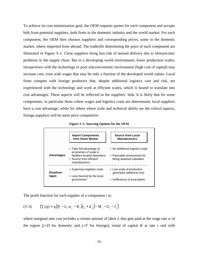
- 50 -

To achieve its cost minimization goal, the OEM requests quotes for each component and accepts

bids from potential suppliers, both firms in the domestic industry and the world market. For each

component, the OEM then chooses suppliers and corresponding prices, some in the domestic

market, others imported from abroad. The tradeoffs determining the price of each component are

illustrated in Figure 3–1. Close suppliers bring less risk of missed delivery due to idiosyncratic

problems in the supply chain. But in a developing world environment, lower production scales,

inexperience with the technology or poor macroeconomic environment (high cost of capital) may

increase cost, even with wages that may be only a fraction of the developed world values. Local

firms compete with foreign producers that, despite additional logistics cost and risk, are

experienced with the technology and work at efficient scales, which is bound to translate into

cost advantages. These aspects will be reflected in the suppliers’ bids. It is likely that for some

components, in particular those where wages and logistics costs are determinant, local suppliers

have a cost advantage; while for others where scale and technical ability are the critical aspects,

foreign suppliers will be more price competitive.

Figure 3–1: Sourcing Options for the OEM

Disadvan-tages

Advantages

• No additional logistics costs

• Favorable environment for being awarded subsidies

• Take full advantage of economies of scale in facilities located elsewhere

• Source from efficient manufacturers

• Low scale of production generates additional cost

• Inefficiency of local plants

• Expensive logistics costs

• Less favored by the local government

Import Components from Home Market

Source from Local Manufacturers

The profit function for each supplier of a component i is:

(3–3) ( )( )iiijjijiii IGMdrKwLPqq −−−+−−=∏ ...)(

where marginal unit cost includes a certain amount of labor L that gets paid at the wage rate w of

the region (j=D for domestic and j=F for foreign); rental of capital K at rate r and with

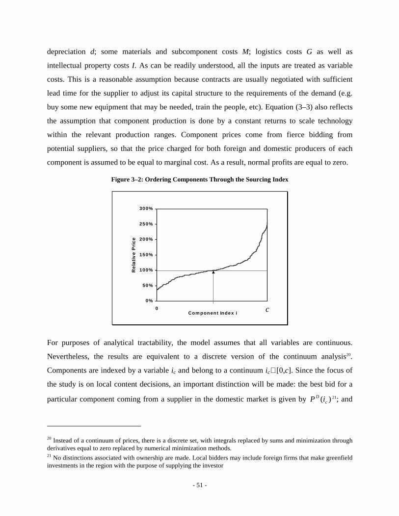
- 51 -

depreciation d; some materials and subcomponent costs M; logistics costs G as well as

intellectual property costs I. As can be readily understood, all the inputs are treated as variable

costs. This is a reasonable assumption because contracts are usually negotiated with sufficient

lead time for the supplier to adjust its capital structure to the requirements of the demand (e.g.

buy some new equipment that may be needed, train the people, etc). Equation (3–3) also reflects

the assumption that component production is done by a constant returns to scale technology

within the relevant production ranges. Component prices come from fierce bidding from

potential suppliers, so that the price charged for both foreign and domestic producers of each

component is assumed to be equal to marginal cost. As a result, normal profits are equal to zero.

Figure 3–2: Ordering Components Through the Sourcing Index

0%

50%

100%

150%

200%

250%

300%

0 274Com ponent Index i

Rel

ativ

e P

rice

c

For purposes of analytical tractability, the model assumes that all variables are continuous.

Nevertheless, the results are equivalent to a discrete version of the continuum analysis20.

Components are indexed by a variable ic and belong to a continuum ic∈ [0,c]. Since the focus of

the study is on local content decisions, an important distinction will be made: the best bid for a

particular component coming from a supplier in the domestic market is given by )( cD iP 21; and

20 Instead of a continuum of prices, there is a discrete set, with integrals replaced by sums and minimization through derivatives equal to zero replaced by numerical minimization methods. 21 No distinctions associated with ownership are made. Local bidders may include foreign firms that make greenfield investments in the region with the purpose of supplying the investor

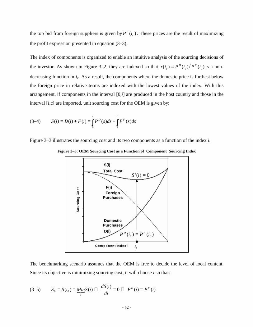
- 52 -

the top bid from foreign suppliers is given by )( cF iP . These prices are the result of maximizing

the profit expression presented in equation (3–3).

The index of components is organized to enable an intuitive analysis of the sourcing decisions of

the investor. As shown in Figure 3–2, they are indexed so that )()()( cF

cD

c iPiPir = is a non-

decreasing function in ic. As a result, the components where the domestic price is furthest below

the foreign price in relative terms are indexed with the lowest values of the index. With this

arrangement, if components in the interval [0,i] are produced in the host country and those in the

interval [i,c] are imported, unit sourcing cost for the OEM is given by:

(3–4) ∫∫ +=+=c

i

Fi

D dssPdssPiFiDiS )()()()()(0

Figure 3–3 illustrates the sourcing cost and its two components as a function of the index i.

Figure 3–3: OEM Sourcing Cost as a Function of Component Sourcing Index

0 274Com ponent Index i

Sou

rcin

g C

ost

Total Cost

Foreign Purchases

Domestic Purchases

i0

)()( 00 iPiP FD =

0)(' =iS

F(i)

S(i)

D(i)

The benchmarking scenario assumes that the OEM is free to decide the level of local content.

Since its objective is minimizing sourcing cost, it will choose i so that:

(3–5) ! )()(0)()()( 00 iPiPdi

idSiSMiniSS FD

i=⇔=⇔==

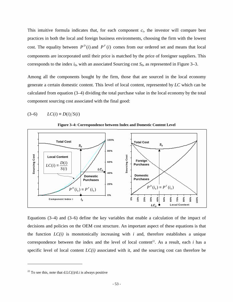
- 53 -

This intuitive formula indicates that, for each component ci, the investor will compare best

practices in both the local and foreign business environments, choosing the firm with the lowest

cost. The equality between )(iP D and )(iP F comes from our ordered set and means that local

components are incorporated until their price is matched by the price of foreigner suppliers. This

corresponds to the index i0, with an associated Sourcing cost S0, as represented in Figure 3–3.

Among all the components bought by the firm, those that are sourced in the local economy

generate a certain domestic content. This level of local content, represented by LC which can be

calculated from equation (3–4) dividing the total purchase value in the local economy by the total

component sourcing cost associated with the final good:

(3–6) )()()( iSiDiLC =

Figure 3–4: Correspondence between Index and Domestic Content Level

0 274Component Index i

Sou

rcin

g C

ost

0%

20%

40%

60%

80%

100%Total Cost

Domestic Purchases

S0

i0

)()( 00 iPiP FD =

LC0)()()(

iSiDiLC =

Local Content

0% 10%

20%

30%

40%

50%

60%

70%

80%

90%

100%

Local Content

Sou

rcin

g C

ost

Total Cost

Foreign Purchases

Domestic Purchases

LC0

)()( 00 iPiP FD =

S0

Equations (3–4) and (3–6) define the key variables that enable a calculation of the impact of

decisions and policies on the OEM cost structure. An important aspect of these equations is that

the function LC(i) is monotonically increasing with i and, therefore establishes a unique

correspondence between the index and the level of local content22. As a result, each i has a

specific level of local content LC(i) associated with it, and the sourcing cost can therefore be

22 To see this, note that d.LC(i)/d.i is always positive

- 54 -

represented also as a function of the level of domestic content. It also generates a ‘natural level’

of local content LC0=LC(i0). This correspondence and the representation of the sourcing cost as a

function of the domestic content are represented in Figure 3–4.

3.2.2. The Effect of Domestic Content Requirements

What happens if the local government requires the OEM to have a certain level of domestic

purchases? The intuitive result, detailed below, is that enacting content requirements will

increase the sourcing cost of the OEM. Because of monopoly pricing, this additional cost will

also result in an increased price for the final good and a reduction in the quantity sold. Both

effects reduce the welfare of the local economy.

When facing local content requirements, the foreign investor will select the components across

the universe of potential suppliers that meet the local content requirement with the least

aggregate cost. Using l as the level of requirement, and considering equations (3–4) and (3–6),

this means that the sourcing decision must verify LC(i)>=l. The new cost minimization objective

of the OEM can be written as23:

(3–7) { }liLCiSii

l ≥= )( :subject to )( minarg"#"$%

The solution to (3–7) establishes that, for a given level of domestic content requirement l

demanded by the government, there will be a set of components in the interval [0,il] that will be

locally sourced inputs and remainder iε(il,c] imported. Clearly, the level of local content

requirements only makes a difference to the economy if 0LCl ≥ . If this is the case, the constraint

in (3–7) is binding and defines the index il. Moreover, because of the monotonicity of LC(i), this

relationship is unique and 0iil ≥ . The new index also defines the sourcing cost as Sl = S(il).

23 This is a definition based only in non-labor input value. Alternatively, the definition could also include labor inputs, profits and taxes as domestic content; a definition based on part count has also been used (see Grossman, 1981)

- 55 -

The sourcing cost of the investor will always be penalized by the extra price of the domestic

components across the distance [i0,il] that needs to be incorporated to meet the domestic

requirements. This implication can be seen graphically in Figure 3–3 or Figure 3–4. As either

index or local content is moved from the level corresponding to the minimum cost towards the

right, the sourcing cost increases. From the definition proposed in equation (3–4), the sourcing

cost difference ∆S = Sl - S0 can be simplified to:

(3–8) ∫ −=∆li

i

FD dssPsPS0

)()(

A change in the OEM sourcing cost will result in a price change following the pricing behavior

described in formula (3–2). For small changes around the maximum, the price correction is given

by ∆P = ∆S/(1+(1/Ed))24. This change will also affect the quantity sold and the profit of the

investing firm according to:

(3–9) tSc

SqEq d −+∆=∆ and ( )

+

∆+∆−=

−+

∆+

+∆−=∆Πdd

dOEM

EMCSq

tScS

EE

Sq11

%11

1

Consumer surplus will also be affected. Without loss of generality, the inverse demand function

is assumed to be approximately linear within the relevant price difference region (this assumption

will also be used in all further calculations of changes in consumer surplus). As a result, one

obtains:

(3–10) ( ) ( )

∆+

+∆−=∆+∆−≅∆ MCE

ESqqqPCS d

d

%211

112/

where the marginal cost is given by MC=c+S-t.

The profit change presented in equation (3–9) has two components. The first is profit erosion due

to additional souring cost and the second is the adjustment due to the change in price and

- 56 -

quantity arising from the monopolistic behavior of the investor. This means that, for levels of

elasticity below -1, quantity sold is reduced and the profits of the investing firm decrease.

Likewise, consumer surplus is reduced both due to the increase in price and the reduction in

quantity. Total welfare, measured through the profits of the firms25, consumer surplus and

government revenue is clearly reduced. This can be written as:

(3–11) 0<∆+∆Π+∆+∆Π=∆ GSCSW SUPOEM

The first two terms are given by equations (3–9) and (3–10) respectively and are negative for

elasticity less than -1. As explained in section 3.2.1, normal profits of suppliers in the domestic

supply chain are always zero, which results in the third term of (3–11) also being zero. Because

there are no direct revenues to the government the last term is not changed with the alterations

due to domestic content requirements.

This conclusion that domestic content requirements on the investing firm (above the natural level

of decision) increase the price of the intermediate goods – the components – and, consequentially

the price of the final good, therefore reducing welfare is accordance with what most previous

authors in the area have also found. Nevertheless, these findings have a crucial dependence on

the assumptions regarding perfect markets, i.e. that all factors are being paid exactly their

marginal cost. As detailed in the next sections, in a developing nation this may not be always the

case. As a result, the welfare implications of the policy may be different from the standard

evaluation presented in the previous paragraphs.

3.3. Benchmarking Domestic Content Policies

The previous section presented the base situation for domestic content requirements, concluding

that such a policy had negative effects on OEM profit and overall country welfare. Although a

subsequent section shows that there may be situations where this policy can be welfare

24 Significant variations in cost will shift the firm maximization point enough to alter the value of the point elasticity in the denominator. As a result, the new price would be calculated with the new elasticity and the formula wouldn’t hold. This situation adds complexity to the calculations offering no additional benefit in intuition.

- 57 -

enhancing, this section compares domestic content requirements with two other situations that

have been as prevalent in the developing world as a means to protect the local industry: tariffs

and subsidies to producers. The relevant conclusion detailed in the next sections is that local

content requirements are potentially superior to tariffs and subsidies as ways to increase the share

of domestic purchases by an OEM. By setting a standard and letting the foreign investor make

the decisions on how to comply, the government benefits from the firms’ ability to minimize

potential negative impacts on its cost and, as a result, the overall economy.

3.3.1. Are Domestic Content Requirements Better Than Tariffs?

The first relevant issue is a comparison of domestic content requirements and tariffs. The idea is

that the government would like to know if reaching a certain level of domestic purchases leaves

the local welfare better (or less worse off) if it is accomplished through a policy requiring the

OEM to achieve this predetermined level of national content or, alternatively, through the

enactment of tariffs on imported components that would displace them in favor of local ones. To

study the problem, a base sourcing structure, cost and natural local content that result from the

minimization process described in (3–5) are assumed. These are represented, respectively, by i0,

S0 and L0. What will be shown is that the following proposition holds:

Proposition. A domestic content requirement policy is weakly preferable to a uniform

price based tariff policy when measured in terms of welfare of the local economy.

Tariffs create a cost penalty on imported components that does not exist for the case of domestic

content requirements. Moreover, this additional burden on sourcing cost is aggravated by the

monopoly pricing of the OEM, further reducing domestic welfare

If the government option is to enact a domestic requirement policy, the result is defined directly

by the mechanisms presented in the previous section. A requirement LCl results in a sourcing

structure il and cost Sl, both defined by equation (3–7). Likewise, the cost penalty ∆Sl = Sl - S0, is

25 For simplicity, assume that all profits remain in the country

- 58 -

given by equation (3–8) and the impact on quantity and welfare by the subsequent formulas. The

total welfare impact of this policy is named as Wl.

Now, instead of the domestic content requirement, consider a tariff that covers all foreign

components equally on a percentage of their purchase price. The calculation of the new sourcing

structure is similar to finding the natural level of local content, but with the foreign price adjusted

by the tariff level. This requires each foreign component price in equation (3–4) to be replaced by

the new sourcing price: )()1()( sPsP FF ζ+→ , with ζ being the tariff schedule.

Using equation (3–5), the result of the minimization process is implicitly given by

)()1()( TF

TD iPiP ζ+= , with iT and ST representing the sourcing structure and associated cost.

Moreover, since the objective is to compare this policy with the domestic content policy, the

government will set the tariff level ζ to make sure that iT is equal to il, assuring that the same

level of ‘true’ domestic content is achieved26. This results in 1)()( −= lF

lD

l iPiPζ . The new

sourcing cost is now:

∫∫ ++=c

i

Fl

iD

l

l

l

dssPdssPiS )()1()()(0

ζ and

(3–12) ( ) ∫∫∫ =++=−=∆c

i

Fl

c

i

Fl

i

i

FDTT

TT

T

dssPTdssPdssPsPiSiSS )( defining ; )()()()()(0

0 ζζ

Comparing equations (3–12) and (3–8), it is easy to note that there is an important difference in

the cost penalties that the OEM is subject to in the two policies. As it can be seen in in Figure 3–

5, charging a tariff shifts both the foreign and total cost curves upwards. Since the tariff can be

set so that iT = il, the domestic content is the same as if LC(il) would be demanded by the

government. Nevertheless, the new sourcing cost is higher than before, with TSS lT +∆=∆ .

This is because all foreign components in the interval [il,c] that are still bought also pay the tariff,

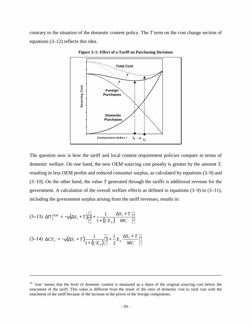
- 59 -

contrary to the situation of the domestic content policy. The T term on the cost change section of

equations (3–12) reflects this idea.

Figure 3–5: Effect of a Tariff on Purchasing Decisions

0 274Com ponent Index i

Sou

rcin

g C

ost

Total Cost

Foreign Purchases

Domestic Purchases

i0 iT

The question now is how the tariff and local content requirement policies compare in terms of

domestic welfare. On one hand, the new OEM sourcing cost penalty is greater by the amount T,

resulting in less OEM profits and reduced consumer surplus, as calculated by equations (3–9) and

(3–10). On the other hand, the value T generated through the tariffs is additional revenue for the

government. A calculation of the overall welfare effects as defined in equations (3–9) to (3–11),

including the government surplus arising from the tariff revenues, results in:

(3–13) ( ) ( )

+∆+

++∆−=∆ΠMC

TSE

TSq l

dl

OEMT 11

11.

(3–14) ( ) ( )

+∆

++

+∆−=∆MC

TSEE

TSqCS ld

dlT 2

11111

26 ‘true’ means that the level of domestic content is measured as a share of the original sourcing cost before the enactment of the tariff. This value is different from the result of the ratio of domestic cost to total cost with the enactment of the tariff because of the increase in the prices of the foreign components.

- 60 -

(3–15) ( )

+∆

+=∆+=∆MC

TSEqTTqqGS l

dT 1

If the effects in the previous formulas are added, it can be shown that the corresponding total

welfare effect is given by:

(3–16) ( )

−∆

++

−∆=∆MC

ETSE

qTWW dl

dlT

2.1

11

Where ∆Wl is the welfare effect obtained through the domestic content policy. Since the elasticity

of demand is negative and below minus one, it is straightforward to see that tariffs penalize the

economy beyond the effect of domestic content requirement, demonstrating proposition 2.

There are two aspects driving this result. The first is that the extra cost penalty on the imported

components, represented by T, does not exist for the case of domestic content requirements.

Second, this additional burden on sourcing cost is aggravated by the monopoly pricing of the

OEM, further reducing profits and consumer surplus. The additional government revenues never

compensate for this effect. As a result, a requirements policy is preferable to the enactment of

tariffs.

The reason why domestic content requirements are only weakly preferable to tariffs comes from

the fact that the tariff policy can be set to replicate the effect of the requirement policy. If the

government gives the tariff revenue back to the OEM in form of a subsidy, then the cost penalty

T is removed from the profit equation and the increase in sourcing cost is reduced to ∆Sl, the

same as in the case of the domestic content. As a result, the pricing does not change and the

welfare effects of the two policies will be equivalent. This result can also be used to assess the

how policy makers can replace one policy by the other.

The intuitive reason leading to the superiority of the content requirement policy is the ability of

the government to use the knowledge of the OEM in choosing components. By imposing the

standard and leaving the component sourcing decision to the company, the government knows

that it is in the firm’s best interest to reach the desired level of domestic purchases with minimal

sourcing cost. This behavior also minimizes any potential negative impact on domestic welfare.

- 61 -

On the contrary, a uniform tariff penalizes all components, even those that have the largest gap

between domestic and foreign production. This extra unnecessary cost creates an additional

welfare burden on the local economy.

Governments have tried to mitigate this problem by establishing selective tariff policies, with

differentiated levels depending on the component (Krueger, 1975; Bennet, 1986; Shapiro, 1993).

Ultimately, if the government would be able to target the components at the margin with tariffs

that compensate exactly for their difference between domestic and foreign production costs, it

could obtain the same result as the one reached though the content requirements policy. The

problem is that governments do not have the necessary information to establish the appropriate

targeting. Moreover, even if that would be possible at one point in time, local market conditions

change over time with new local supplier investments, typically at a faster pace than the

government can follow. As a result, it becomes impossible in practical terms to use tariffs as an

alternative to content requirements without further reducing welfare.

3.3.2. Subsidies and Domestic Content Requirements

Now the objective is to compare domestic content requirements with a policy of awarding a

uniform subsidy to all local manufacturers. The analysis of the domestic content requirements is

similar to what was shown in the previous section. Nevertheless, unlike the analysis of the tariff

policy, it will not be possible to reach an overall conclusion on the comparison.

A direct subsidy based on a percentage σ of the component cost is considered. Since domestic

suppliers will be pricing at the new marginal cost, the new price for each component is replaced

by )1( σ−→ Di

Di PP . Using (3–4) and (3–5), the OEM minimizes the sourcing cost so that

)()()1( SF

SD iPiP =−σ , with iS and associated SS representing the sourcing structure and

associated cost. This scenario is very close to the one analyzed in the previous section for the

case of tariffs. The major difference is that, instead of moving the foreign components cost curve

upwards, the domestic components cost curve is shifted downwards, generating a new

equilibrium. This situation is presented in Figure 3–6

- 62 -

Figure 3–6: Effect of a subsidy on Purchasing Decisions

0 274Com ponent Index i

Sou

rcin

g C

ost

Total Cost

Foreign Purchases

Domestic Purchases

i0 iT

Since, like in the case of tariffs, the objective is also to reach a level of domestic content identical

to a direct restriction, the subsidy level is decided so that iS = il. This results in

)()(1 lD

lF

l iPiP−=σ . The new sourcing cost is now:

∫∫ +−=c

i

Fi

DlS

S

S

dssPdssPiS )()()1()(0

σ and

(3–17) ( ) ∫∫∫ −=−+=−=∆s

s

T iD

c

i

Fi

i

FDsS dssPBdssPdssPsPiSiSS

00 )( defining ;)()()()()(

0

σσ

Analyzing this equation, one can see that that its structure is identical to the analysis that was

performed in the case of tariffs. Therefore, equations (3–13) to (3–16) can be directly applied in

this context, replacing T by B27. The problem with the new calculations is that, because B is

negative, the numerator of the right hand side term of equation (3–16) can be either positive or

negative, depending on the relative values of the parameters. As a result, little can be said

regarding which of the two policies hurts the economy less. Moreover, this evaluation is bound to

become even more complex if one considers that there may be additional costs associated to

27 In the government surplus calculation, a cost of raising the money might have to be added.

- 63 -

raising the subsidy money, and that not all the profits of the OEM are retained in the domestic

economy.

3.4. Externalities and the Social Evaluation of Domestic Content

As discussed in detail in chapter 2, the prospect for local companies in developing nations to

participate as suppliers of components for complex products such automobiles, capital goods or

electrical units is often unique and seen as a critical opportunity to gain the experience and

recognition that will enable the local industry to increase overall productivity28. This situation

may generate a gap between the social and private cost of the resources that are employed in

suppliers, with their social opportunity cost below the private cost. This is the key difference to

the situation analyzed in previous sections.

In a free market environment the OEM will choose the lowest (quality adjusted) price for each

component. This generates the base sourcing structure i0, a sourcing cost S0 and a resulting

natural level of local content, represented by LC0. This natural local content generates surplus to

the domestic economy, designated by W0. If the government enacts local content regulations then,

the company makes the least cost supplier choice subject to the LCR policy, resulting in a new

sourcing structure of the firm il, sourcing cost S0 and welfare Wl.

The issue is to understand the conditions under which these regulations are beneficial to the

country, focusing on the economic welfare effects of the policy29. Welfare calculations include

producer surplus, both generated by the OEM (OSP) and the suppliers (SSP), consumer surplus

(CS) and government surplus (GS). Therefore, welfare can be written as:

(3–18) GSCSSSPOSPW +++= and GSCSSSPOSPW ∆+∆+∆+∆=∆

28 A similar reasoning can be made if the foreign OEM induces foreign suppliers to invest in the country instead of contracting local firms, since foreigners often bring unique knowledge that may partially spillover to the local economy 29 if one is to abstract from political effects

- 64 -

Following the discussion of section 3.1, two different analyses are presented. The first

investigates how government should consider local content requirements in the presence of a

generic gap between the social and private opportunity costs of the resources used in the industry.

The second models a situation where industry spillovers exist based firms and industry

experience, but they are unaccounted by private firms. It will be shown that, if a foreign OEM

investing in a developing economy generates unaccounted learning and spillovers effects that

depend on the breadth of the supplier structure, local content requirement can improve welfare as

long as the unaccounted benefits of the components sourced beyond the OEM market decision

are above the cost penalty associated to them.

3.4.1. Differences in Private and Social Opportunity Costs

The key idea of this scenario is that, although OEM and suppliers have to pay input factors

according to their private cost, this value is above their social opportunity cost. This also reflects

the major difference between this model and the work of other authors, since previous research

has mostly neglected the possibility that factors may not be paid their social marginal cost.

Section 3.1 explained how external effects can be interpreted as a reduction in social opportunity

costs below the values paid by the private agents. The relevant factors included labor and capital,

as well as disembodied technology, which will be associated with development expenditures.

Since it is difficult to have accurate estimates of the opportunity cost for the resources allocated

to a particular project, they will be made parameters. Based on equation (3–1) and (3–3), the

following corrections are considered:

• The social opportunity cost of each unit of labor is given by (1-λ).w

• The social opportunity cost of each unit of capital is given by (1-φ).r

• The social opportunity cost of intellectual property is given by (1-π).I

Following the social cost benefit approach, the welfare effect of a project is reassessed by

considering the social opportunity cost of the resources, instead of the private cost. Taking into

- 65 -

account the profit function presented in equation (3–1)30, annual surplus for the OEM can now be

written as:

(3–19) ( )tKrLwqOSP OEM −++Π= φλτ , with τ as the tax rate

In addition to the OEM surplus, purchases of components in the local economy also generates

producer surplus. Like the investor firm, the contributions of these firms are potential profits and

the social value of the factor inputs used in production. Using the profit equation (3–3), the

surplus that each domestic firm i can generate if included as a supplier is:

(3–20) ( ))()()()()( iIriKwiLqiiSSP πφλ +++Π=

where Π(i) represents normal profits that are zero for the supplier behavioral assumptions that

have been described before. The total surplus derived from the participation of local suppliers is:

(3–21) ∫=i

dssSSPSSP0

).(

The government surplus is also affected through the subsidies that are awarded to the firms.

What is important to reflect on is that the opportunity costs for government funds is often greater

than its monetary value. The reason for this situation is the fact that these funds have to be

collected through taxes that distort the economic decision making (Laffont and Tirole, 1993,

chapter 2). As a result, government surplus is now given by:

(3–22) tqGS )1( ψ+−=

where ψ is the additional cost penalty of raising government funds.

These adjusted calculations for producer and government surplus, added to consumer surplus

(that does not have to be adjusted because of the differences in opportunity costs noted above)

result in the new value for the total welfare of the local economy. As noted before, since this

30 This evaluation can be further refined by considering the negative effect of expending foreign exchange.

- 66 -

research addresses the effect of domestic content requirements, the focus is on variations of

welfare from the base decision with no content requirements, as opposed to a calculation of

absolute welfare values.

Section 3.2.2 explained that an OEM that is prevented from buying components from less

expensive foreign manufacturers because of domestic content requirements will have higher

sourcing costs. As shown in equations (3–9) and (3–10), this leads to lower profits and

diminished consumer surplus. Under social cost benefit analysis, these negative surplus

calculations have to be balanced against the positive surplus generated by the difference between

social and private valuations of the resources, reflected on the right hand side terms of equations

(3–19) and (3–20). This is the key tradeoff that becomes relevant to analyze.

The analysis of this tradeoff is greatly simplified if it is assumed that the government uses

subsidies to compensate the OEM for the higher sourcing costs. If this happens, the OEM cost

remains equal before and after the enactment of the local content requirements. As a result, the

final good price will also remain constant and so will the quantity produced, the OEM profits and

the consumer surplus. As seen below, the advantage of assuming this compensation is that it

allows the mathematical simplification while retaining the characteristics of the key tradeoff that

is the focus of this section. Moreover, Chapter 4 shows that the strategy of compensation can be

an optimal solution for the problem from an incentive perspective. Therefore, for the remaining

of the section, it will be assumed that the government pays any penalty that results from its

content policies.

Under this simplification, the new welfare changes resulting from a local content policy can be

written as:

(3–23) 0=∆SSO ; ( )∫ ++=∆li

i

dssIrsKwsLqSSP0

.)()()( φλ ; 0=∆CS ; tqGS ∆+−=∆ )1( ψ

and St ∆=∆ to offset the increased cost from greater incorporation of local suppliers.

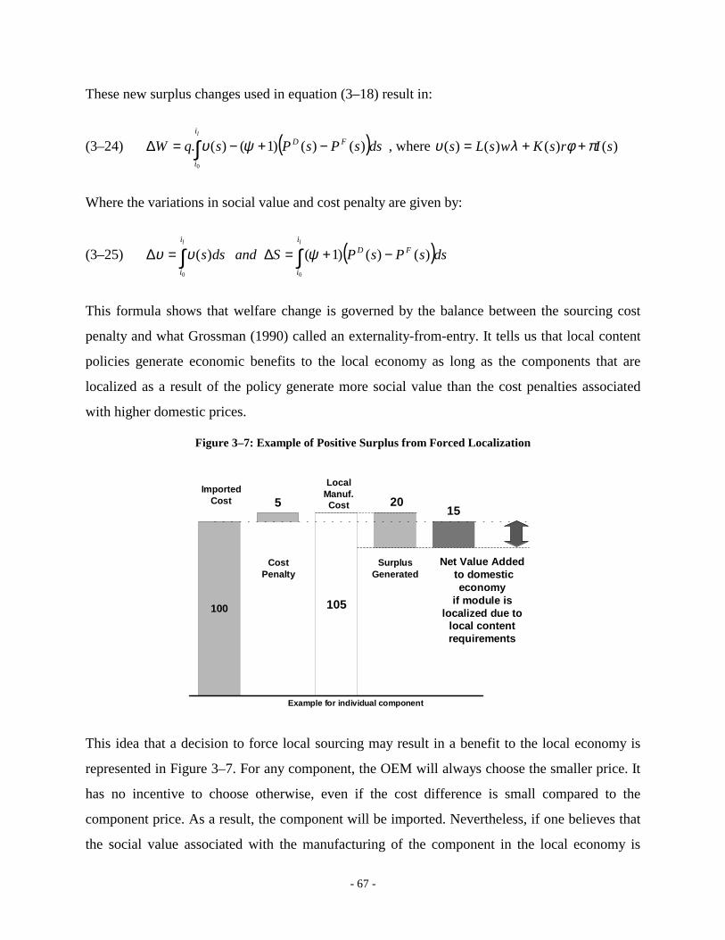
- 67 -

These new surplus changes used in equation (3–18) result in:

(3–24) ( ) dssPsPsqWli

i

FD∫ −+−=∆0

)()()1()(. ψυ , where sIrsKwsLs )()()()( πφλυ ++=

Where the variations in social value and cost penalty are given by:

(3–25) ( ) dssPsPS and dssll i

i

FDi

i∫∫ −+=∆=∆00

)()()1()( ψυυ

This formula shows that welfare change is governed by the balance between the sourcing cost

penalty and what Grossman (1990) called an externality-from-entry. It tells us that local content

policies generate economic benefits to the local economy as long as the components that are

localized as a result of the policy generate more social value than the cost penalties associated

with higher domestic prices.

Figure 3–7: Example of Positive Surplus from Forced Localization

105

15

100

5 20Local

Manuf.Cost

ImportedCost

CostPenalty

SurplusGenerated

Net Value Addedto domestic economy

if module is localized due to

local content requirements

Example for individual component

This idea that a decision to force local sourcing may result in a benefit to the local economy is

represented in Figure 3–7. For any component, the OEM will always choose the smaller price. It

has no incentive to choose otherwise, even if the cost difference is small compared to the

component price. As a result, the component will be imported. Nevertheless, if one believes that

the social value associated with the manufacturing of the component in the local economy is

- 68 -

greater than the cost penalty, the economy would be better off if this difference would be

subsidized to allow domestic purchase. This is precisely what the policy on local content

requirements coupled with the government subsidies to offset the cost penalty does.

A careful analysis of the expression (3–24) describing the welfare effects of a policy requiring

domestic content also shows that there is an optimum associated with the enactment of such a

policy. In fact, a sound administration of the policy should require an investing OEM to localize

components not while the welfare change is positive, but rather while welfare is growing.

Differentiating expression (3–24) with respect to il, one gets31:

(3–26) ( ))()()1()(0.

. WF

WD

Wl

iPiPiidWdWMax −+=⇔=∆⇔∆ ψυ

Equation (3–26) is intuitive and tells that local components should be added until the cost penalty

of the marginal component reaches its social value. This is equivalent to localizing components

until the marginal return to the government equals the marginal cost to the firm. This equation

also enables the following proposition:

Proposition. In the presence of a gap between private and social valuations of the

resources employed in potential suppliers of an OEM, a small domestic content

requirement policy coupled with an OEM subsidy for the cost penalty can be welfare

enhancing.

To see why this has to be true, equation (3–26) is rearranged as

)()1()(1)()( WF

WWF

WD iPiiPiP ++= ψυ . This implicitly defines the index that maximizes

welfare when there is some extra social value to the local economy. Since, both the index and the

level of domestic content increase with the ratio )()( WF

WD iPiP , any positive value of )( Wiυ

moves the index towards the incorporation of more local components, i.e. iW > i0, with i0

corresponding to the decisions with 0)( =iυ . Therefore, any l<LC(iW), with LC(i) defined as in

equation (3–6), will increase welfare.

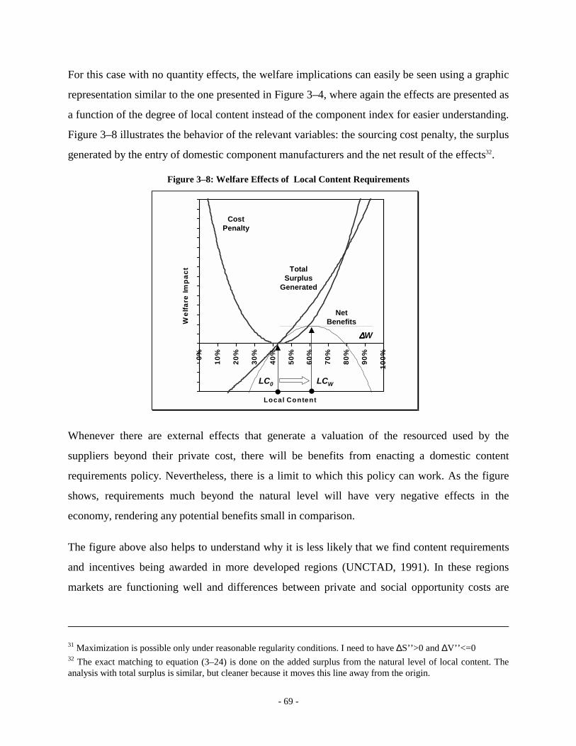
- 69 -

For this case with no quantity effects, the welfare implications can easily be seen using a graphic

representation similar to the one presented in Figure 3–4, where again the effects are presented as

a function of the degree of local content instead of the component index for easier understanding.

Figure 3–8 illustrates the behavior of the relevant variables: the sourcing cost penalty, the surplus

generated by the entry of domestic component manufacturers and the net result of the effects32.

Figure 3–8: Welfare Effects of Local Content Requirements

0% 10%

20%

30%

40%

50%

60%

70%

80%

90%

100%

Local Content

Wel

fare

Impa

ct

LC0 LCW

∆∆∆∆W

Cost Penalty

TotalSurplus

Generated

Net Benefits

Whenever there are external effects that generate a valuation of the resourced used by the

suppliers beyond their private cost, there will be benefits from enacting a domestic content

requirements policy. Nevertheless, there is a limit to which this policy can work. As the figure

shows, requirements much beyond the natural level will have very negative effects in the

economy, rendering any potential benefits small in comparison.

The figure above also helps to understand why it is less likely that we find content requirements

and incentives being awarded in more developed regions (UNCTAD, 1991). In these regions

markets are functioning well and differences between private and social opportunity costs are

31 Maximization is possible only under reasonable regularity conditions. I need to have ∆S’’>0 and ∆V’’<=0 32 The exact matching to equation (3–24) is done on the added surplus from the natural level of local content. The analysis with total surplus is similar, but cleaner because it moves this line away from the origin.

- 70 -

usually much smaller. Therefore, the surplus curve will be shallow and its slope will rapidly

match the slope of the cost penalty, limiting the region where there may be positive benefits from

enacting domestic content requirements.

3.4.2. Learning and External Effects

So far all costs and prices have been constant regardless of the sourcing decisions of the OEM.

Nevertheless, given that the issue that is at the core of the thesis are spillovers in the supply

chain, it is important to address how they may change the conclusions that have been reached so

far. If the hypothesis is that local firms learn with experience and that there may be external

effects present in the decisions, it is important to address those directly in the formulation. The

interest is to understand how learning changes the ability of the local government to demand

local content requirements. To perform the desired analysis, the standard base case with no

learning is compared against several learning patterns to understand how the sourcing structure

and, more importantly, the welfare impact changes with the rate of learning.

First, firm learning-by-doing is explored. Experience with a particular manufacturing technology

renders improvements in efficiency that eventually result in cost improvements. The influential

paper by Arrow (1962) established this issue as critical in the economics and management

literature. Since then, this hypothesis has been explored in the literature, both at a theoretical

(Lieberman, 1987; Mody, 1989) and an empirical level (Lieberman, 1984; Lamoreaux, Raff et

al., 1999; Sinclair, Klepper et al., 2000). Virtually all of these studies report that cost decays

exponentially with cumulative output of the company over time.

The second type of learning that will be considered is learning-by-spillovers. The idea is that

manufacturing costs of individual firms may be reduced as the presence of other related

companies in the region increases. Factors such as the ability to exchange information and solve

technical problems in common, share workers among companies and the development of

regional technical centers are all bound to have a positive effect in the manufacturing capability

of the firms and, therefore, on their cost. Like the case of the learning by doing, most authors

have suggested that the appropriate representation of the phenomenon is an exponential driven by

the cumulative output of the relevant industry.

- 71 -

Given previous work, the following formula can used to represent these two effects:

(3–27) γβα −−= itititi YXC

Where Cit is the cost of component i at time t, Xit is the learning-by-doing index and Yit represents

learning-by-spillovers. The interest is in finding an appropriate way to model these in the context

of the problem under analysis. The main complication arises from the fact that a monopolist

whose costs change due to learning should have a strategic behavior, charging less than the

monopoly price in initial stages to increase output and take better advantage of the learning effect

(Lieberman, 1987; Tirole, 1988, p. 72). This strategic effect makes the analysis much more

complex, with no substantial gains in terms of intuition or the overall magnitude of the results.

Therefore, a simplified version of this problem is considered. The simplifying assumption is to

have quantity decided before the investment takes place, so that it can’t be changed throughout

the project33. This eliminates the effects of strategic behavior and monopoly pricing. If this is the

case, then output quantity is constant. What might change depending on the relative cost

structure and government policy is the relative share of components that are produced by local

and foreign suppliers.

Within these assumptions, measuring firm internal learning is rather straightforward, with the

learning-by-doing index established as tqYit .= . This representation is equivalent to having cost

as a function of firm cumulative output, as seen in the studies mentioned before. The above

representation results from the fact that yearly production is assumed constant. The formula

means that doubling the value of cumulative output reduces cost by 2−γ. For example, if γ is equal

to 0.1, the cost reduction is 93%. This number is often treated in the literature as the slope of the

learning curve.

Following the previous literature, learning spillovers will be an exponential function of industry

cumulative output. Since quantity is constant, the number of components manufactured in the

domestic market will drive this indicator. Therefore, the learning index can be written as

33 Generalizing the analysis to include strategic pricing will part of future research

- 72 -

tiqX it ..= . This representation means that every additional component sourced locally adds to

the industry cumulative output and makes an equal contribution to the learning index. Likewise,

every year adds to the index the output corresponding to the total number of domestic

components manufactured in the region.

Once the two indeces are substituted in equation (3–27), and adjusting for the appropriate α, the

result is:

γβ −−= titCC iti )..(0 , t>0

The quantity is dropped from the formula because it is assumed to be constant throughout the

periods34. Taking in consideration that the suppliers’ price is equal to cost, learning can be

accounted in the decision of the OEM by making the following substitution in (3–4):

(3–28) ∫∫ −−→i

Di

D dssPtitdssP00

)().()( γβ 35

The new OEM cost structure depends on time. But, so far the model set-up is static and therefore

not directly amenable to the incorporation of a time framework. Therefore, to fully consider this

issue, the project is assumed to have a certain time horizon over which a net present value is

calculated.

Like the case of quantity discussed above, an optimal solution is described by equation (3–5)

with the replacement indicated in (3–28), taking in consideration strategic effects that influence

monopolistic pricing. Once again, all decisions regarding domestic content will be done before

the project. Nevertheless, while a constant quantity is an important simplification of the real

situation, an up-front decision on suppliers is actually likely. Due to search and approval times

34 This has another underlying simplification that the base quantity manufactured every year does not influence the rate of learning. Therefore, a firm producing 35,000 units will see its cost decrease from the base value at the same rate as another firm manufacturing 70,000 units. The base cost of the two firms will obviously be different. 35 Note that the exponential is left out of the integral to make sure all the components are equally affected by the external effect. If it would be inside, each component would have its cost reduced as a function of its individual position in the ordered index.

- 73 -

and processes (see Veloso, Henry et al., 2000, chapter 3 for the case of the auto industry) there

are usually important switching costs associated with changing a supplier. As a result, the most

likely situation is to consider that the sourcing structure has to be decided up-front and will be

maintained for the duration of the project.

Given the set of assumptions described in the previous paragraphs, the cost structure with

learning effects can be represented through a variation of equation (3–4) according to the

following formula:

(3–29) ( )∑ ∫∫=

+−

++=

n

t

c

i

Ft

iD

tt dssPdssPiST

1 0

1 )()(1)( δ

Where δ is the yearly discount rate; FFt PP = ; )()(1 sPsP DD = and )().()( 0 sPtitsP DD

tγβ −−= for t

greater than 1; n is the number of years of the project. An analysis of this equation rapidly shows

that the above formula yields a scenario that is close to the calculations and the solution for the

case of subsidies discussed in section 3.3.2.. The difference is that the discounting in equation

(3–29) interacts with the learning effect in each period.

With a complete decision before the project, the solution for the new sourcing problem results

from the minimization of ST(i) with respect to i. The problem is that the new equation does not

have an obvious closed form solution. As a result, numerical methods have to be used to find the

appropriate distinction between domestic and foreign components, and the associated iL. In any

case, given that domestic cost decreases over time, the solution for this new problem leads to

more local sourcing than the static no learning calculation. Therefore, the new equilibrium value

iL will be to the right of the original decision i0 presented in section 3.2. This means that the

OEM will source more domestic components. Eventually, this minimization will also be subject

to domestic sourcing requirements.

If the OEM recognizes that learning is taking place, then it will follow the formulas described

above and incorporate them into the decision making process. As a result the government will

have no role to play and domestic content will at most hurt the industry. The problem is learning

effects may become external to the OEM and suppliers decisions, often because firms can’t

- 74 -

anticipate the patterns of individual and collective learning. If this is the case, the local content

resulting from the firm private decisions will be below the socially desirable outcome. As a

result, the government may intervene. It can either subsidize local firms in anticipation of the

difference between private and social costs, or subsidize the OEM while enacting domestic

requirements that bring the share of domestic purchasing to the socially desirable level.

Comparison of these scenarios and the implication of the rate of learning are discussed in the

model application presented in chapter 7. Several values of the parameters β and γ will be tested,

aiming to understand how learning may affect the OEM sourcing decisions and the need or

opportunity for government regulation. As we will see in the numerical calculations these two

types of learning are important and can reinforce the perceptions put forward in the previous

sections, whereby a gap between private and social valuations of the resources used in the

supplier sector may justify government intervention through domestic requirements and

subsidies.

Despite these results, both learning paradigms considered in this section are generally unintended

consequences of the activity, i.e. they are more of a side result rather than a consequence of

purposeful activities. This leaves out another crucial component of learning, the one that results

from purposeful activities that the company undertakes to be able to excel at a particular area.

The problem is that a careful analysis of these issues requires a full dynamic environment with an

incentive structure for the investment in learning, as well as a mechanism for that to happen. This

will be considered as future research.

3.5. Model Extension: Cost Uncertainty and Risk Averse Managers

The previous analysis considered that all prices put forward by the suppliers are deterministic, or

that they correspond to the expected value of a random variable, with the OEM being a risk

neutral player. This section investigates what happens if the costs of local suppliers are a random

variable and the decision maker is risk averse.

Although firms are often considered risk neutral in the economic literature, managers are not. In

the context of the model explored in this chapter, this becomes an issue if a risk averse

- 75 -

purchasing manager makes the OEM sourcing decisions. The problem is that suppliers in a

developing region often have less control over the manufacturing process than their foreign

counterparts. This may lead to unanticipated cost overruns, quality and delivery problems, among

other problems. Any of these have negative impact on the financial outcome of OEM operations.

For simplicity reasons, it is assumed that any problems associated with sourcing from a domestic

supplier have a sourcing cost equivalent that is factored in by the OEM as the perceived domestic

cost. Given the risk averse behavior, it is clear that this manager would prefer to source from a

foreign supplier that he knows will provide a certain cost for sure (e.g. because of past supply

experience) than from a local supplier whose expected cost might be the same as the foreign

supplier, but still has a positive probability of generating costs overruns.

To model this situation the usual assumptions in the literature in terms of the shape of the utility

function and the cost distribution are used. The price of the imported components FiP will be the

same and assumed with certainty. The value of local components are now considered a random

variable RiV = i

DiP ε− with the random component ε representing cost overruns from the

expected value. ε is considered to have a normal distribution with mean zero and variance 2iσ .

The sign is reversed in ε because the manager values less cost. The value can then be represented

as ),(~ 2i

Di

Ri PNV σ .

The manager has a utility function that represents its attitude towards cost savings and cost

penalties. The shape of the utility function is assumed as a constant absolute degree of risk

aversion, represented by xrexu .)( −−= , where x is the level of value savings ( RiVx = ) and r is a

parameter that measures the degree of risk aversion. Since x is assumed to have a normal

distribution, it has been shown36 that the expected utility of the local components cost can be

represented by [ ] 2.)( 2xrxxuE σ−≡ . If the definitions given above are used, the cost of each of

the local parts can be replaced by 2. 2i

rPP Di

Di εσ+→ . With this new representation, the impact

of potential management risk averseness in the sourcing options of the firm can be addressed.

36 See for example Varian (1992), p. 189

- 76 -

The risk averse behavior is equivalent to having the foreign manager demand a price premium

from local suppliers to hedge for the fact that they may have or cause cost overruns. This is

actually a situation that many local suppliers, potential entrants in the industry complain about,

often feeling discriminated against when compared to established firms (Veloso, Henry et al.,

2000). The manager base sourcing structure i0 and cost S0 that result from the normal risk neutral

choice can be compared with the risk averse result iR and corresponding SR. It is easy to notice

that SR>S0 because the ‘adjusted’ perception of the manager is that local suppliers are more

expensive than their expected price. This is equivalent to shifting the domestic supply cost curve

presented in Figure 3–3 upwards. As a result he will substitute some components that would be

sourced by a risk neutral manager in the local market with those produced by a foreign supplier

that are more expensive for sure. This will hurt both the OEM and the local industry.

Here the government could intervene and establish a preemptive domestic content requirement.

Imagine that the government recognizes that there may be risk averseness from the management.

As a response it establishes a level of domestic content that is exactly l=LC0 . Faced with this

new constraint, the risk averse manager has to go back to the sourcing options that would be

made by the risk neutral manager. The domestic content counters the risk averse behavior of the

manager.

The idea is that by enacting local content requirements but compensating these with subsidies,

the government is acting as an insurer of the investor. The reason why the government needs to

intervene is because there is an external cost. The OEM does not want to pay the insurance cost

because it has alternative suppliers in the foreign market at no extra cost, and the individual

firms’ local suppliers may not be willing to pay for it because they may not acknowledge or be

aware that this risk exists. As a result, government intervention may be the only solution.

This section provides an important conclusion to policy makers: establishing domestic content

objectives during the contract negotiation stage can be important to minimize the impact of

potential risk averseness from the managers in charge of sourcing decisions. It is likely that high-

level decision makers negotiating the project with the government within the global portfolio of

the company have a behavior that is closer to risk neutrality than the manager that ends up in

charge of negotiating specific contracts.

- 77 -

3.6. Summary

This chapter proposes a model to benchmark the effects of a local content requirements policy on

the investment of a particular OEM and on the welfare of the economy. Impact is measured based

on welfare or surplus generated by the project, including the effects of any restrictions,

comparing the benefits generated through the investment to those that would be created if the

same resources were deployed elsewhere in the economy. The model is explored at two levels.

First, competitive decisions are analyzed. This enables an understanding of the underlying

decision mechanisms associated with OEM sourcing decisions and a benchmark evaluation of

the impact of a LCR policy on economic agents and on welfare. The analysis includes a

comparison with alternative policies, in particular tariffs and subsidies. The relevant conclusion

is that content requirements is a superior policy to tariffs and subsidies as a means to increase the

share of OEM domestic purchases. By setting a standard and letting the OEM make the decisions

on how to comply, the government benefits from the firm’s ability to minimize potential negative

impacts on its cost and, a result, on the overall economy.

Second, the model studies how the existence of gaps between private and social opportunity costs

of the resources employed in the OEM and its suppliers affects the impact of LCR on the

domestic economy. The analysis shows that local content requirements can improve welfare as

long as the opportunity cost gap of the components sourced beyond the OEM market decision is

above the cost penalty associated with them. The key idea underlying the model is that a foreign

OEM investing in a developing economy generates unaccounted learning and spillovers effects

that depend on the breadth of the supplier structure. This effect generates an externality-from-

entry associated with domestic suppliers that drives the gap between social and private valuation.

The model also describes an extension related to risk aversion from the OEM. It is shown that a

foreign manager may demand a price premium from local suppliers to hedge for the fact that they

may have cost overruns, which decreases domestic sourcing. Content requirements can help to

avoid the behavior of the manager and improve domestic welfare.

- 78 -

Chapter 4. Performance Standards, Information and Content Decisions

Chapter 3 discussed a set of conditions that could engender the need or opportunity to establish

domestic content requirements. As explained, in the presence of differences between social and

private opportunity costs of the resources used by domestic suppliers, or external learning effects,

the domestic economy would be better off if an OEM is forced to source more domestic

components than it would choose if the decision was market based. This chapter analyzes the

mechanisms that can be used by the government to induce the OEM to choose the level of

domestic purchases that yield maximum welfare to the local economy. In particular, it explains

how content requirements coupled with subsidies may be used as performance standards that

drive the OEM to make this optimal choice for the economy. The first section explains how

content requirements and subsidies may work together as performance standards and discusses

the intuitive mechanism that supports the interplay between the two aspects. The second section

describes the formal incentive model, both with full and asymmetric information. The third

section presents policy implications.

4.1. Content Requirements and Subsidies as Performance Standards

4.1.1. Understanding Performance Standards

Governments in industrializing nations have been aware that long-term economic growth

requires local firms to master the technologies of the developed world. chapter 2 explained that

attracting foreign firms to invest locally and promoting the exposure of domestic companies to

international markets is likely to be important for this development process. Nevertheless,

coordination problems, learning and spillovers lead to differences between social and private

opportunity costs for the resources that may result in under-investment by both local firms and

foreign investors in the types of skills and technologies that are critical for industrialization. The

model explained how, under a set of conditions, the optimal sourcing level for the OEM might be

- 79 -

less than what would be optimal for the domestic economy. As a result, the enactment of some

degree of local content requirement could improve domestic welfare.

The discussion of chapter 2 shows that governments in most late industrialized nations

intervened in the economy whenever they perceived the potential for a gap between private and

social costs. Nevertheless, intervention appears to have been more successful in regions such as

Korea or Taiwan, where requirements related to domestic content (but also to other activities

such as exports or technology purchases) were coupled with subsidies and other non-pecuniary

benefits granted to the companies affected by the policy. These policies established incentives

based on reciprocity principles, capable of enhancing learning and development in the economy.

Likewise, case studies on the impact of domestic content policies suggest that these seemed to

have had a better effect whenever used in a discretionary form and bundled with incentive

packages. This articulate effort of coupling requirements with incentives is what will be labeled

as using performance standards for targeted development, which is the focus of this chapter.

Although policy studies reviewed in Chapter 2 have shown that incentives and requirements on

foreign investment are often used together, researchers have mostly considered this juxtaposition

as ambivalence from local governments and not as a deliberate policy mechanism. Therefore, it is

not surprising to note that the reviewed research work on domestic content requirements has not

considered the possibility of balancing subsidies with requirements. Figure 4–1 helps to

understand how the dominant perspective on the role of incentives and requirements (the focus is

on domestic content) does not encompass the idea of performance standards. As the explained

below, the third quadrant has often been left out of any discussion in the subject37.

Most research labels policies related to high levels of requirements as protectionist mechanisms

for inefficient domestic industries, placing them in the fourth quadrant. This has been particularly

prevalent in what concerns domestic content policies. Papers studying the problem consistently

describe models where the critical feature is the fact that the marginal costs of the critical inputs

become greater in the host country than in the international market as a result of the content

37 Guisinger (1989) considers both restriction and incentives, but his focus is on measurement of the joint impact on profitability rather than on the welfare to the local economy

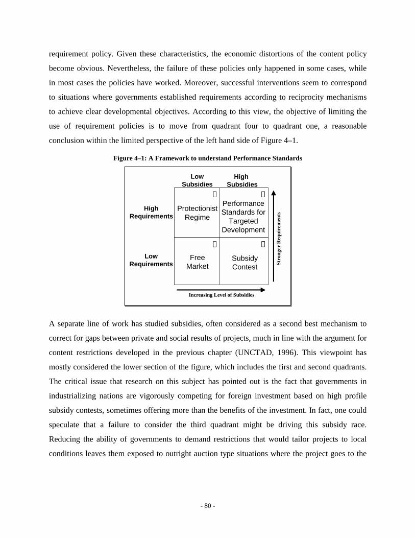
- 80 -

requirement policy. Given these characteristics, the economic distortions of the content policy

become obvious. Nevertheless, the failure of these policies only happened in some cases, while

in most cases the policies have worked. Moreover, successful interventions seem to correspond

to situations where governments established requirements according to reciprocity mechanisms

to achieve clear developmental objectives. According to this view, the objective of limiting the

use of requirement policies is to move from quadrant four to quadrant one, a reasonable

conclusion within the limited perspective of the left hand side of Figure 4–1.

Figure 4–1: A Framework to understand Performance Standards

LowSubsidies

HighRequirements

LowRequirements

➊ ➋

➌➍

High Subsidies

Stro

nger

Req

uire

men

ts

Increasing Level of Subsidies

FreeMarket

SubsidyContest

PerformanceStandards for

TargetedDevelopment

ProtectionistRegime

A separate line of work has studied subsidies, often considered as a second best mechanism to

correct for gaps between private and social results of projects, much in line with the argument for

content restrictions developed in the previous chapter (UNCTAD, 1996). This viewpoint has

mostly considered the lower section of the figure, which includes the first and second quadrants.

The critical issue that research on this subject has pointed out is the fact that governments in

industrializing nations are vigorously competing for foreign investment based on high profile

subsidy contests, sometimes offering more than the benefits of the investment. In fact, one could

speculate that a failure to consider the third quadrant might be driving this subsidy race.

Reducing the ability of governments to demand restrictions that would tailor projects to local

conditions leaves them exposed to outright auction type situations where the project goes to the

- 81 -

region that offers greater subsidies. Economic theory predicts that this will result in the investor

capturing the whole surplus generated by the project38.

This work specifically addresses the third quadrant, evaluating conditions for a successful use of

incentives and requirements to enhance learning and improve development. The government

wants to solve the problem of under-investment by creating the right incentive structure for local

firms and foreign firms entering the country. It sets targets and requirements to firms in the

domestic market that may improve social welfare, and is willing to commit the resources to

compensate the negative effect that its policies may create in economic agents. The argument

explored is that subsidies and requirements coupled through reciprocity principles act as

incentive and screening mechanisms that lead the firms to perform the desired social objectives

by aligning their decision with the optimal for the economy. As before, the focus will be in the

enactment of domestic content requirements.

Within the context of these ideas, one might think that the model discussed in chapter 3 justifies

protectionist measures for a particular context. Yet, section 3.4.1 notes that the government pays

the OEM for any cost penalty associated with the domestic content requirement. This is the

critical assumption that frames the problem as an interplay between requirements and incentives

rather than a mere protectionist policy. In fact, the conclusion of the model is precisely that,

within an optimal incentive contract, the government should pay the OEM exactly its sourcing

cost penalty.

4.1.2. Using Performance Standards to Establish Incentive Contracts

The idea is that the government may use both restrictions and incentives to account for the

difference between the private and social opportunity costs to maximize welfare. The

technological characteristics of a project will determine different cost structures for domestic and

foreign components, as well as for the external benefits associated to domestic purchases. As a

result, each project will vary, both in the natural level of domestic purchases, as well as in the

38 Considering the effect of competition between governments for the project is an interesting extension of the model presented in this chapter that will not be pursued in the thesis.

- 82 -

cost penalty resulting from a content level beyond its natural level. It is in government’s interest

to demand requirements and award incentives to the firm according to the cost of responding to

the social objective function. A project with higher costs to increase domestic content will need

greater subsidies to respond to an equivalent level of social objectives than another with lower

costs.

In a standard model, both the company and the government are aware of each other’s objective

functions, costs and how they vary with domestic content (this was the case for the model in

Chapter 3)39. Therefore, it is intuitive to think that a reasonable approach is for the government to

demand content requirement beyond the natural level and to compensate the company for this

extra effort until the marginal social benefit equals the marginal cost. What will be shown in the

next section is that the optimal incentive contract is for the government to offer the OEM a

subsidy that varies according to the level of domestic content that it chooses. This contract can be

set up so that the OEM chooses the content level that is optimal from the point of view of the

domestic economy and receives a subsidy that will match the cost penalty due to the extra

domestic purchasing. An important conclusion is precisely the fact that the optimal subsidy is

equivalent to the cost penalty, the assumption considered for the model of Chapter 3.

In the real world, a government facing a potential investment may not be sure of how costly it is

for the OEM to increase domestic content beyond the natural level. It also may not know exactly

what benefit it derives from increasing domestic sourcing. Therefore, it becomes difficult to

establish the optimal contract. Suppose that, upon entering a negotiation with a prospective

investor in the region, the government is unable to know ex-ante the cost to the firm of an

increase in the level of domestic content. Nevertheless, lets consider that costs will be either high

or low and that the government knows the probability of each of them. Now imagine the

government proposes an optimal contract (with a schedule of subsidies and a corresponding level

of domestic content) that is aimed at the expected costs and benefits of the average firm. If the

company faces a low cost to increase domestic content, it will gladly take the offer, since

subsidies will cover more than its cost. On the other hand, if the company has a cost of

39 The specific intuition described from here onwards is formalized in the model presented in the next section

- 83 -

compliance above average, it will under invest, or may choose not to invest at all if the level of

content demanded becomes more costly than the subsidies given out by local government. This

situation is what the economics literature generically describes as an adverse selection problem.

The superior information of the firms, in particular the ability of the low cost firm to mimic the

behavior of high cost one generates a rent for the low cost or under investment from the high cost

firm.

To better understand this problem a case where the intrinsic value of the project is rather

important (even with no externalities), and the government wants to make sure that the

investment takes place for both the high and the low cost firms, is assumed. This is a rather

plausible scenario for a large OEM investment in a developing country. If government doesn’t

know the true cost for the companies to comply with content requirements (but knows the cost

distribution) and can only offer one bundle of requirements and incentive, the solution is to offer

the bundle directed at the high cost firm, that has less domestic content requirements and also

awards less money. Under these circumstances the firm with high cost will take the offer. But so

will the low cost one, for which it is less costly to respond to the regulation. The problem is that

this solution is not efficient because the government could be better off with a different

arrangement in content requirements and incentives directed at the low cost firm.

The adverse selection problem highlighted above can be minimized (although not eliminated, as

seen below). The government can offer a menu of two bundles, letting the firm choose the one it

prefers. The menu should have both a strong domestic content requirement coupled with a large

incentive, and a small requirement with an associated limited incentive. Moreover, the values can

be adjusted so that the bundle with demanding requirements and a large incentive looks more

attractive to the low cost firm than the lower requirements with corresponding low incentives.

Faced with this menu of choices, the firms self-select themselves when maximizing their profits.

For the firm with the high costs of compliance with content requirements, the best choice is to

choose the bundle with low content requirements and small incentives, while for the low cost

firm the natural choice is the aggressive requirement and large incentive. In this situation, the

allocation is more efficient than before where only one bundle was offered.

- 84 -

4.2. The Formal Model

The ideas outlined above can be formally expressed through a variation of the adverse selection

model well established in the literature (Laffont and Tirole, 1993; Mas-Colell, Whinston et al.,

1995, ch 14.; Salanié, 1997, ch 2). The government wishes to maximize local returns from the

investment of a particular company in its country or region. The idea is that these returns depend

on the type of company and its level of effort expensed in tailoring its operations to fit the needs

of the local economy. In many ways, the model presented below can be thought of at as an

extension of the one developed in chapter 3. Nevertheless, the regularity conditions that have to

be imposed here are much stronger. Therefore, the analysis is treated as stand-alone and the

necessary parallels to the work presented in the previous Chapter are drawn whenever necessary

to understand the links between them.

This model also adds to the growing body of literature that explores the role of asymmetric

information on strategic trade policy. Existing models have addressed the effects of the

asymmetric information in Brander and Spencer (1985) rent-shifting trade type models (Qiu,

1994; Brainard and Martimort, 1997; Kolev, 1997). They concluded that information problems

weakens the ability of the government to gain domestic welfare advantages through subsidies,

with the degree of this effect depending on the influence of the actual characteristics of the

market. The conclusions of the model presented here follow a similar pattern.

The objective of the firm is to maximize profits. These include two components. The first is the

intrinsic value of the project, which corresponds to the original motivation to undertake the

investment. For the purpose of our study, this is considered to be the profit associated to the basic

project, labeled as Π0. The second component is the net result of the incentive given by the

government minus the additional costs faced by the project as a result of the extra level of

domestic content demanded by the government (equivalent to the ∆S described in equation (3–8)

of Chapter 3 multiplied by the quantity sold). These costs depend on the effort demanded through

the level of content requirement, as well as on the type of firm. So, one gets:

Firm additional profit: ),(),( ββ eSteE −=Π

- 85 -

Where e represents domestic content requirement beyond the natural level, β represents firm type

and t is the subsidy awarded from the government to the firm.

The marginal cost of compliance with additional content requirements is assumed to increase

with the firm inefficiency in increasing content level. This can be written in mathematical form

as 0),(,0),(,0),(,0),(,0),0(,0),0( ''''''' >>>>== ββββββ ββ eSeSeSeSSS eeeee . For the above

assumptions to be coherent, a larger β will be associated with a firm facing higher cost of

compliance with domestic content requirements.

Following the ideas developed in chapter 3, the domestic economy will receive a certain surplus

associated with increasing local purchases (equivalent to the supplier surplus defined in equation

(3–24) of chapter 3). This can be represented as:

Government revenue: ),( βeV

Where revenue grows with content level e, but with diminishing returns, i.e.

0),(,0),( ''' ≤≥ ββ eVeV eee .

The government also has a cost. This is the cost of any subsidy it pays the firm to make sure it

achieves the extra content desired (the government surplus in the same equation 26). Like before,

this cost is corrected to account for the penalty of raising money from taxpayers. Therefore, the

cost is represented as:

Government cost: tC )1( ψ+= ,

Where t is the subsidy paid to the company and ψ the additional burden of raising money.

The full expressions for both the government and the firm are:

Firm: ),(),,( 0 ββ eStte −+Π=Π

Government: teVteG )1(),(),,( ψββ +−=

- 86 -

4.2.1. Base Case: First Best

Now the objective is to understand how the relationship between the two parties is established.

First, a base case is established, against which any relevant variations will be evaluated. In the

base case the types of firms and content levels are common knowledge. This is the traditional

neoclassical problem. The government will maximize surplus minus cost, subject to the

participation constraint (PC) of the firm (i.e. the firm will only invest if the offer of the

government is better than an outside option with value Π0). This is equivalent to:

),,(:,

teGMaxte

β

(PC) s.t. 00 ),(),,( Π≥−+Π=Π ββ eStte

or, assuming that the restriction is binding,

)),(()1(),(:,

βλψβ eStteVMaxte

−−+−

Differentiating with respect to e and t, the result is, respectively:

),(),( '' βλβ eSeV ee −= and λψ =+− )1(

The result is:

(4–1) ),(1

),( *'*'

βψ

β eSeVe

e =+

This result tells us that the government should choose a level of domestic content so that the

marginal cost for the firm to comply with the requirements equals the marginal benefit for the

government. To assure that the firm chooses the appropriate level of effort, the government offers

the firm the following contract:

(4–2)

+

−+

+=ψβ

ψβββ

1),(

1),(),(),(

** eVeVeSet

- 87 -

The profit maximizing behavior results in the government awarding the firm ),( * βeSt = , and

the firm responds with the level of domestic content e* defined in equation (4–1). When this is

the case, the participation constraint (PC) will be binding. This result also matches the

conclusion presented in equation (29) of Chapter 3. In addition, it shows that the optimal solution

is indeed to pay the OEM exactly the additional cost it has to endure to comply with regulation,

leaving it indifferent between the new solution and the original contract.

This initial result provides us some additional insights:

• Linear incentive contracts may be efficient. It is usually difficult for the government to assess

the complete value curve V of the project for society. Nevertheless, it is straightforward to see

that if the value curve ),( βeV in equation (4–2) is replaced by )*,(. ' βeVe e , the result will be

the same. This means that the information the government may need is reduced, requiring it

to know the level of content requirement it wants to achieve, the value of these benefits at the

maximum and the slope of the variations around this optimal level. Under these

circumstances, the government will offer the firm a contract of the form ebat .+= . This

shows that very simple linear performance standard contracts can be efficient from the point

of view of the firm and the domestic economy.

• In more developed regions it is less likely to find content requirements and incentives being

awarded. In more developed regions, a particular investment project is one of many others.

Therefore, the government is more likely to be mostly concerned with having the project

happen, but has little or no value for additional effort. Therefore, its returns can be interpreted

as containing the firm profit, with a marginal benefit from the additional effort likely to be

very small (i.e. ),(),(),( βββ eMeeV +Π= , and 0),( →βeM ; this implies 0),(' →βeVe ).

As a result, both e* and t(e*) will go to zero. This conclusion is in line both with the

conclusions of chapter 3 and earlier findings on this issue (UNCTAD, 1991).

• It is not surprising to see governments establishing similar incentives schemes for similar

projects. When the government learns the structure of the cost of compliance with domestic

- 88 -

content requirements, it can anticipate the reaction of the firms and, therefore, offer the

corresponding incentive schemes.

• Tax collection affects the ability of the government to improve domestic welfare. Equations

(4–1) and (4–2) indicate that the level of content demanded from a firm and the

compensation offered by the government are affected by the cost of raising government funds

(the parameter ψ). Therefore, higher costs of government funds will reduce its ability to offer

incentives and will mean that a lower level of content will be demanded from a given firm.

• The uniqueness of the investment opportunity affects the ability of the firm to demand

incentives to compensate demands of higher content. If the government becomes aware that

the outside option of investment is below the opportunity in its region (i.e. PC becomes 00 ),(),,( outette Π≥−+Π=Π βψβ and 00

outΠ>Π ), then the government can reduce its

incentives by the same amount of the difference between the base result for the firm in the

region and elsewhere.

4.2.2. Asymmetric Information: Second Best

Now the situation where the government is not aware of the firm type at the time of negotiation

is analyzed. For simplicity, two possibilities for the types of firms are considered. The first will

face a lower cost to comply with domestic content regulations while for the other it will be more

costly to respond40. This is can be written as:

β : Low cost

β : High cost

Since the government knows it may be dealing with two types of firms, it will generate different

offers, which consist of bundles of incentives and content requirements. These will be called

),( et and ),( et , considering that the first set is aimed at firms with type β , while the second tries

40 This can be generalized for a continuum of types. See for example Salanié (1997)

- 89 -

to respond to the type β company. Moreover, although the government is not aware of the firm

type, it will have a prior probability that it is facing either a low cost or high cost firm. The

distribution considered is:

ξ = Prob. (β= β )

1-ξ = Prob. (β= β )

The government maximization problem can now be considered. Given the assumptions outlined

above, it will maximize the expected value of its result:

(4–3) [ ] [ ]teVteVMaxtete

)1(),()1()1(),(:,,,

ψβξψβξ +−−++−

This maximization will be subject to a set of constraints. These include the participation

constraint for each firm. The new versions of equation PC presented above are:

(PC1) 00 ),(),,( Π≥−+Π=Π ββ eStte

(PC2) 00 ),(),,( Π≥−+Π=Π ββ eStte

In addition to these, there are two additional constraints. These are called incentive compatibility

constraints (ICC). The idea is that whenever a firm chooses a contract, it should be better off with

the particular level of requirement and incentive it chooses, and would prefer to pretend to be the

other type of firm and get its contract. If the model specification is considered, this means:

(IC1) ),(),( ββ eSteSt −≥−

(IC2) ),(),( ββ eSteSt −≥−

- 90 -

It can be shown that the solution for this problem is (see Appendix 9.1.1 - calculations for

asymmetric information):

(4–4) For β : )(1

),(1

),( *'*'*'

eeSeVe

e Φ−

+=+ ξ

ξβψ

β

(4–5) For β : ),(1

),( *'*'

βψ

βeS

eVe

e =+

Where ∫=−=Φβ

ββ ββββ deSeSeSe eee ),(),(),()( '''''

So, the optimal strategy for the government is to offer the firm a menu of contracts with two

bundles ),( ** et and ),( **et 41 that are determined by the equations (4–4) and (4–5). If the new

equilibrium solutions are compared with (4–1), it is possible to see that they yield an efficient

level of effort from the low cost firm, coupled with a positive rent, as well as underprovision of

effort from the firm with higher cost to comply with regulations. Because the low cost firm may

mimic the behavior of the higher cost firm, the government gives up some rent if it wishes to

have the firm with high costs also investing in the region.

Like before, there are some additional implications of the results:

• If the government is aware that the firms are either mostly low cost or high cost, then

contracting becomes efficient. This means that ξ−>1 or ξ−>0, respectively. As a result, one

goes back to the situation where the government is aware of the characteristics of the firms. It

also builds a case for the developmental government to have a good understanding of an

industry. The better it understands it, the better it can tailor the menus.

41 Alternatively, it could offer two contracts with )),(())()(()(),(^^

*'^

*^^

*^

ββββββ eSeetet e−+= , { }βββ ,^

=

- 91 -

• The more dissimilar the types of firms, the more inefficient contracting can get to be. This is

due to the structure of Φ’(e), where increasing differences in the type characteristics (i.e. β -

β ), or a steep marginal cost difference between the two firm cost type (i.e. 0),('' >>ββ eSe )

forces the government to further lower the level of content requirement demanded from the

high cost firm to give more rent to the low cost firm.

4.2.3. Deviations From Optimal Behaviour

First, the study considers what happens if the government is limited in its ability to demand

performance requirements. This is a crucial aspect because there is increasing pressure from the

WTO for the developing world to drop performance requirements it has traditionally demanded

from certain types of investments.

• If content requirements are prohibited, the firm extracts incentives from the government until

project benefit is zero or there will be no offer from the government.

For any of the firm types, the best strategy is to demand the subsidies upfront announcing that it

will endure the content level desired by the government and then set extra content to zero and

still keep the government funds. To see how this may happen consider that, without an effort

provision, the return for the government is a tax α on firm profit minus the cost of incentives

given out to the firm42. Under these circumstances, the firm will maximize:

),(),,(: 0

,ββ eStteMax

te−+Π=Π s.t. 0)1()),((),,( 0 ≥+−−+Π= teStteV ψβαβ . The

solution for this problem is to set e=0 and demand t=α Π0/(ψ+1-α). So V=0, and Π>Π0.

Nevertheless, the government may anticipate that the firm will not comply with the desired

content level if it is not forced to and may decide not to offer any incentive at all.

• If the government is not able or allowed to discriminate between firms and can only offer one

type of contract, two things may happen. The contract will either be tailored for the high cost

firm and there will be underprovision of effort, or the government will offer the bundle aimed

42 Formally this means that we have to consider that V(0,β)>0

- 92 -

at the low cost firm, which will deter the high cost firm from investing (all calculations

presented in Appendix 9.1.2).

Lets assume that the government maximizes the expected value of the returns, subject to

participation constraints of the firms43.

[ ] [ ]teVteVMaxte

)1(),()1()1(),(:,

ψβξψβξ +−−++− s.t. 00 ),( Π≥−+Π βeSt , βββ ,=

The solution is for the government to offer a contract so that:

(4–6) ),()1()(.),( '' βψξβ eSeBeV ee +=+ ,

with βββ

ββ deVeB e ),()( ''∫−= being the additional marginal utility that the government gains from

having a the low cost firm deriving the effort. Therefore, the exact solution depends on the

structure of B(e).

- If it is only the level of domestic content that drives the benefit, i.e. ),('' ββ eVe =0, then

B(e)=0 and one gets ),()1(),( *1

'*1

' βψβ eSeV ee += . Therefore, the government will choose

a contract that is optimal for the high cost firm. The low cost firm will respond by

mimicking the high cost one, and extract the extra rent derived from the fact that

complying with domestic content is less costly to it.

- If the marginal result for the government increases with firm efficiency, i.e. 0),('' <ββ eSe ,

then B(e)>0 and the result is ),()1()(.),( *2

'*2

*2

' βψξβ eSeBeV ee +=+ . Comparing this result

with the one of the previous paragraph, it can be concluded that *1e < *

2e . The government

increases the content requirement with increases in the likelihood of a low cost firm and

the difference between marginal benefits.

43 Without differentiated offers, there is no incentive compatibility constraint. It’s a take it or leave it offer.

- 93 -

- But the government will choose to shut down the high cost firm if the expected benefits

of having this type of firm doing the project are below the result the government is giving

away for the other type. In this situation, the government will always require a high level

of content commitment, offering the appropriate high incentives. In this situation, the

project will only happen if the firm is of the low cost type, but the effort of the firm will

be efficient. This happens either because the revenue of the high cost firm is too low, or

because the rent derived by the low cost firm is too high. Mathematically, this effect is

driven by a very large difference in marginal benefit between low and high cost firms.

In any of the cases, it is obvious to see that the inability of the government to observe or to

demand different performance requirements to the firms dampens their level of commitment to

the economy and, as a result, the benefits that the government derives from their investment.

4.3. Summary

This chapter analyzes the mechanisms that can be used by the government to induce the OEM to

choose the level of domestic purchases that yield maximum welfare to the local economy.

Subsidies and content requirements coupled through reciprocity principles act as incentive

mechanisms that align OEM decision with the optimal choice for the domestic economy. When

offered the adequate options with bundles of content requirements and subsidies, companies will

self-select themselves in an optimal way while correcting for the gap between social and private

benefits and costs. Nevertheless, the analysis also shows that uncertainty on how the enactment

of content requirements affects the cost structures of the firms reduces the ability of the

government to enact efficient incentive contracts and to improve domestic welfare.

The incentive model described in this chapter works as an extension of the work presented in

chapter 3 (although stronger regularity conditions are necessary for the formal proofs). In fact, for

the case with full information, the conclusions of both models converge, and the incentive

contract results provide the necessary justification for the assumption used in chapter 3 of having

the cost penalty of the investing firm paid by the government.

- 94 -

These results also provide a good understanding for some of the findings of earlier studies

mentioned in chapter 2, which suggest that, despite its pervasive presence, performance standards

do not greatly affect in the decisions of investing companies (UNCTAD, 1991). In fact, given the

results exposed above, firms that choose to enter a market with performance standards, where

subsidies and requirements are used to correct for coordination problems and external effects, are

doing so because it is optimal for them and for the local economy.

- 95 -

Chapter 5. SCM - System Cost Modeling

As seen in previous chapters, understanding the decisions of investing firms and local

governments in what concerns domestic content depends heavily on component cost structures in

the relevant market contexts. In particular, it is important to know how the manufacturing

conditions in the developing nation contrast with those found in the world market to be able to

investigate on the trade-offs between local and foreign sourcing. The problem is how to assemble

cost information for all the relevant components that are subject to the OEM sourcing decisions.

For an automobile, for example, this could mean hundreds of components, for which price

information from two locations would have to be gathered. Even if it would be possible to find

these prices, they would pertain specific manufacturing condition and would not allow sensitivity

analysis to changes in relevant variables such as volume or cost of capital.

The alternative solution is to model the cost for these components. The establishment of a cost

structure for all the components that takes in consideration their use of factor inputs such as

materials, labor and capital, would enable an analysis of the OEM sourcing decision. Moreover,

if it would account for aspects such as factor costs, logistics conditions and production volume, it

would also enable the desired examination of the influence of regional manufacturing conditions

on cost and, consequentially, on the local content decisions and policies.

To be able to make this assessment, this chapter proposes a methodology to evaluate the cost of

complex systems with a large number of individual components and subsystems. First it

describes the existing techniques for estimating cost and their relative advantages and

disadvantages. Then it describes a new methodology called Systems Cost Modeling (SCM) that

proposes a number of simplifications that enable it to be used to build bottom-up cost structures,

starting at the level of the individual component and aggregating cost to the subsystems and

system level. The main advantage of this approach is that it requires relatively few inputs per part

making the task of estimating cost of large numbers of parts more manageable.

- 96 -

5.1. Manufacturing Cost Modeling

The issue of manufacturing cost estimation has long been a source of concern for managers and

researchers (see Sims, 1995 for a full review of issues associated to manufacturing cost

estimation). Several techniques have been proposed to estimate cost. While initial ones were

rather crude and served mainly to provide rough orders of magnitude, increasing cost and profit

pressures in the industry during the later part of this century have generated the necessity for

more precision in the estimates. This section reviews the main techniques that have been used to

assess manufacturing cost, discussing their main objectives, characteristics and limitations.

Rules of Thumb

The best known techniques for evaluating the cost of manufacturing processes are simple rules of

thumb. Designers or engineers with experience with the relevant technologies and processes

usually develop rules of thumb (Busch and Field III, 1988). They are often based on two of the

core cost drivers of any manufacturing activity: materials cost and cycle time.

• Markup over materials cost. In many manufacturing processes, materials are an important

share of the total cost. Experience in a particular industry enables experts to accurately

predict this share and suggests the development of rules that are easy to understand by

everyone and provide results that are sometimes close to the actual cost of the component.

For example, the material costs for steel stampings is expected to be something between

50% and 80% of the total cost, depending on part geometry (see for example German,

1998; Veloso, Henry et al., 2000).

• Materials cost plus shop time burden. This technique acknowledges that, in addition to

materials, processing time is another major cost driver for manufacturing. Processing time

cost is then characterized through a burden associated with part production cycle time.

This burden can include an estimated machine and tool rent, cost for the workers

associated with the production process, etc.

There are three major problems with these rule of thumb techniques. First, they rely heavily on

historical data and previous experience. Therefore, they have strong limitations in environments

- 97 -

of rapid change in materials, technologies and customer requirements. Second, they assume

linear relationships between factors driving cost. This leads to misleading results as in most

situations these relations are fundamentally non linear. Third, these are black-box techniques that

do not allow the manager to understand the interplay between the several factors that are driving

cost, nor do they allow experiments to understand potential cost savings. As a result, relying on

rules of thumb to make important technical or managerial decisions can be extremely misleading

and costly to the company.

Accounting Principles

Cost estimation by accounting principles uses current accounting data and practices in the plant

to estimate manufacturing cost. A particularly popular application of these principles is activity

based costing (ABC), which attributes direct and overhead costs to products and services on the

basis of the underlying activities that generate the costs (Cooper and Kaplan, 1988). When

successfully applied, ABC has enabled a better understanding of the cost drivers and more

accurate decisions of pricing and marketing decisions. It may also provide accurate estimates of

equipment and workers burden rates (Anderson, 1995). Nevertheless, it has been of limited help

to engineers and designers concerned with improving the manufacturing lines or choosing

between alternative materials. The reason for this situation is that ABC is based on historical and

descriptive information, and seldom incorporates any engineering control variables. Therefore, it

retains some of the fundamental ex-post characteristics of rules of thumb, hampering the

possibility to establish predictions for new manufacturing systems, materials or part

characteristics.

Econometric analysis

This estimation process involves assuming a predetermined functional form for production,

either stemming from a theoretical proposition or empirical observations, and then regressing the

dependent variable (cost or quantity) on the relevant independent ones (regressions are typically

linearized forms of non-linear relationships).

Econometric estimation has been used to study a wide variety of aspects, including economies of

scale on production, monopolistic pricing, productivity differences and quality of labor and

- 98 -

capital efficiency measured by embodied technical progress, among many others (Pesaran and

Wickens, 1997). The analysis, nevertheless, looks at the industry or sector aggregation level, with

individual firms as an observation for the regression. Therefore, while this technique has

provided economists with relevant information to understand aggregate behavior, it provides

limited predictive information in situations of changes in the underlying technological process,

and it does not facilitate the individual decision makers in the firm. Moreover, although some

attempts to include relevant engineering information in economic production functions have been

made (Wibe, 1984), the economic and engineering professions have mostly become more far

apart, and limited work integrating the two perspectives has been tried.

Technical Cost Modeling

The problem with the previous techniques is the fact that they offer very limited power for

estimating the effects of departures from observed conditions in manufacturing cost. These

limitations led to the development of Technical cost modeling (TCM) methodology at the

Massachusetts Institute of Technology in the late seventies (Busch and Field III, 1988; Clark,

Roth et al., 1997; Kirchain and Clark, 2001). TCM is related to the activity based costing idea of

accounting principles, but uses engineering, technical and economic characteristics associated

with each manufacturing activity to evaluate its cost.

TCM analysis starts with an identification of the relevant process steps required to manufacture a

particular component. The fender of a vehicle, for example, may start as a steel sheet that is

blanked, then stamped, and later painted. For each identified step, all cost drivers are estimated.

TCM evaluates fixed and variable costs separately. This division reflects the fact that variable

costs can be directly associated with the production of one unit of output, thus increasing roughly

linearly with production volume. On the contrary, fixed costs remain constant until production

capacity is reached, whereupon more equipment is required. These categories are then subdivided

into variable costs of material, direct labor, and energy; and the capital costs of main and

auxiliary equipment, tooling, building, maintenance and overhead. These items reflect those used

in classical accounting methods in order to maintain consistency with conventional views on

cost. The critical difference with the accounting approach is that values underlying each of the

- 99 -

categories are a reflection, not of accounting information gathered at a plant, but of how

engineering process knowledge influences each of these cost accounts.

TCM is a flexible tool to analyze the manufacturing cost implications of different strategies,

business conditions and product characteristics. The models enable wide experimentation and

analysis, critical to evaluate relative strengths and weaknesses of alternative paths, or to pinpoint

critical engineering or economic factors affecting cost, particularly in early stages of design.

TCM and other techniques that are closely related, provide rather accurate estimates of the

manufacturing cost and have been used with success in a number contexts (Boothroyd, Dewhurst

et al., 1994; Humphreys and Wellman, 1996; Clark, Roth et al., 1997; Ulrich and Pearson, 1998;

Kirchain and Clark, 2001).

Because the systems cost model that is the object of this chapter relies heavily on the TCM

approach, a more detailed explanation of this method is presented, which is then used to ground

the SCM explanation presented in section 5.3.

5.2. Technical Cost Modeling

As noted above, TCM uses engineering knowledge to estimate relevant cost drivers associated

with relevant cost drivers for each processing step required to manufacture a particular

component. This section explains the TCM approach used to calculate each of these drivers and

how technical knowledge is incorporated in the calculations. The division between fixed and

variable costs highlighted above is used, followed by a discussion of the equally important

concept of time usage of equipment. At the end, a discussion of the limitations and extensions of

TCM is presented. More detail on the method can be found on Busch (1988), Clark (1997) or

Kirchain (2001).

5.2.1. Fixed Costs

Fixed costs are associated with aspects of the process that cannot easily be changed within the

time frame relevant for the analysis, and are independent of the level of our control variables or

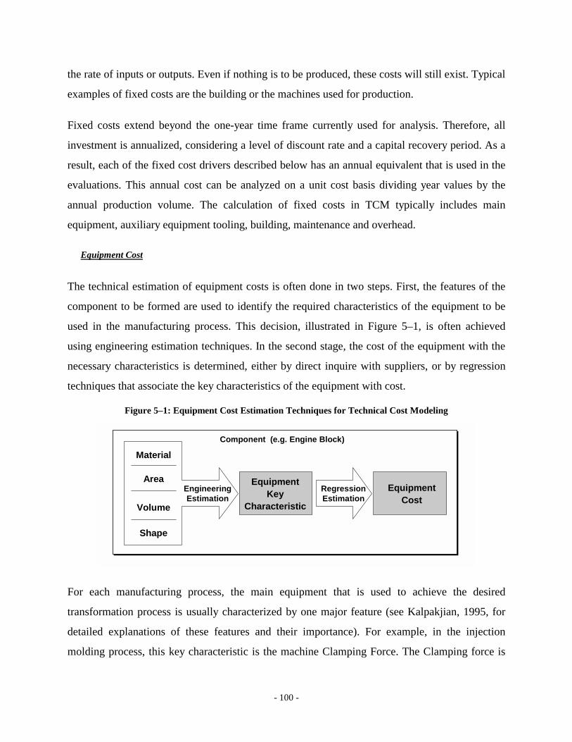
- 100 -

the rate of inputs or outputs. Even if nothing is to be produced, these costs will still exist. Typical

examples of fixed costs are the building or the machines used for production.

Fixed costs extend beyond the one-year time frame currently used for analysis. Therefore, all

investment is annualized, considering a level of discount rate and a capital recovery period. As a

result, each of the fixed cost drivers described below has an annual equivalent that is used in the

evaluations. This annual cost can be analyzed on a unit cost basis dividing year values by the

annual production volume. The calculation of fixed costs in TCM typically includes main

equipment, auxiliary equipment tooling, building, maintenance and overhead.

Equipment Cost

The technical estimation of equipment costs is often done in two steps. First, the features of the

component to be formed are used to identify the required characteristics of the equipment to be

used in the manufacturing process. This decision, illustrated in Figure 5–1, is often achieved

using engineering estimation techniques. In the second stage, the cost of the equipment with the

necessary characteristics is determined, either by direct inquire with suppliers, or by regression

techniques that associate the key characteristics of the equipment with cost.

Figure 5–1: Equipment Cost Estimation Techniques for Technical Cost Modeling

EquipmentKey

Characteristic

Component (e.g. Engine Block)

Material

Volume

Area

Shape

EngineeringEstimation

RegressionEstimation

EquipmentCost

For each manufacturing process, the main equipment that is used to achieve the desired

transformation process is usually characterized by one major feature (see Kalpakjian, 1995, for

detailed explanations of these features and their importance). For example, in the injection

molding process, this key characteristic is the machine Clamping Force. The Clamping force is

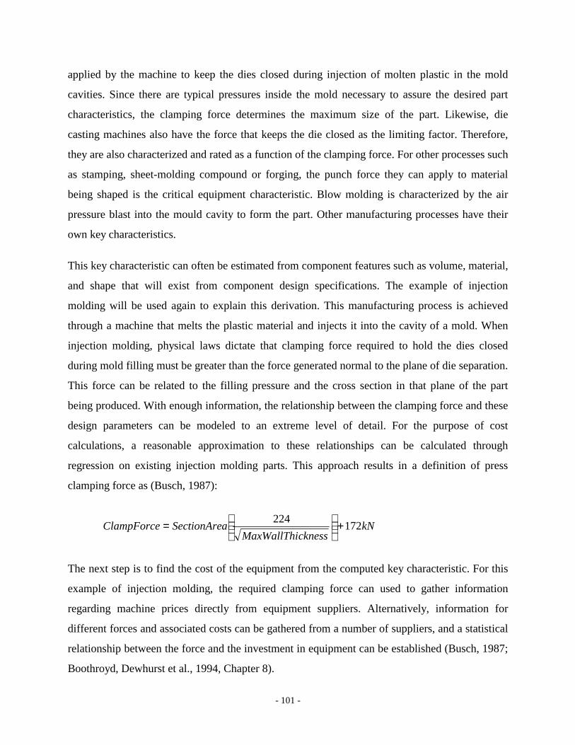
- 101 -

applied by the machine to keep the dies closed during injection of molten plastic in the mold

cavities. Since there are typical pressures inside the mold necessary to assure the desired part

characteristics, the clamping force determines the maximum size of the part. Likewise, die

casting machines also have the force that keeps the die closed as the limiting factor. Therefore,

they are also characterized and rated as a function of the clamping force. For other processes such

as stamping, sheet-molding compound or forging, the punch force they can apply to material

being shaped is the critical equipment characteristic. Blow molding is characterized by the air

pressure blast into the mould cavity to form the part. Other manufacturing processes have their

own key characteristics.

This key characteristic can often be estimated from component features such as volume, material,

and shape that will exist from component design specifications. The example of injection

molding will be used again to explain this derivation. This manufacturing process is achieved

through a machine that melts the plastic material and injects it into the cavity of a mold. When

injection molding, physical laws dictate that clamping force required to hold the dies closed

during mold filling must be greater than the force generated normal to the plane of die separation.

This force can be related to the filling pressure and the cross section in that plane of the part

being produced. With enough information, the relationship between the clamping force and these

design parameters can be modeled to an extreme level of detail. For the purpose of cost

calculations, a reasonable approximation to these relationships can be calculated through

regression on existing injection molding parts. This approach results in a definition of press

clamping force as (Busch, 1987):

kNcknessMaxWallThi

aSectionAreClampForce 172224 +

=

The next step is to find the cost of the equipment from the computed key characteristic. For this

example of injection molding, the required clamping force can used to gather information

regarding machine prices directly from equipment suppliers. Alternatively, information for

different forces and associated costs can be gathered from a number of suppliers, and a statistical

relationship between the force and the investment in equipment can be established (Busch, 1987;

Boothroyd, Dewhurst et al., 1994, Chapter 8).

- 102 -

This type of relationship is much more powerful than an accounting estimate since it enables a

rather accurate estimate of the relevant cost driver from related design variables across a wide

range of conditions. Moreover, this type of estimation method can be performed for virtually any

technology, with the relevance of each design parameter depending on the particular process

under consideration (see Han, 1994; Kirchain, 1999 for a discussion of the multiple applications

of TCM). If instead of injection molding, the above consideration would be for stamping, the

relevant component features to estimate the punching force would be material, area and the depth

to length ratio.

The equipment cost estimated through the steps described above usually has to be adjusted to

take in consideration two aspects. First, auxiliary equipment cost may have to be considered.

Quotes from equipment suppliers often do not include complementary machinery such as

fixtures, conveyors and workbenches, among others. Because it extremely difficult to have an

accurate estimation of these costs, they are usually considered as a percentage of the investment

in the main equipment, with ranges depending on the level of automation that will be used to

loading, unloading and conveying. These values are usually gathered directly using industry

estimates. The second correction is for installation costs. Any industrial equipment requires

careful installation, ranging from electrical power and dedicated supplies to precise positioning in

the building and training of the workers. These are relevant additional costs beyond the

equipment value. Like auxiliary equipment, they are difficult to estimate and are usually

considered to be a fixed percentage of the equipment cost.

Another important element of equipment cost is tooling. Tooling cost is probably the most

difficult value to estimate because it is unique for each part that is produced. The main difficulty

arises from the inability to completely describe tool complexity using only limited and standard

component description inputs. A small geometric detail can make a tool extremely difficult to

produce and, therefore very expensive. The approach used with more success is to regress tooling

cost on certain material, geometric, durability and conformability characteristics of the tool,

based on historical information for each relevant process (Busch, 1987; Busch and Field III,

1988; Boothroyd, Dewhurst et al., 1994, chapter 8 to 10).

- 103 -

Although tooling is also considered an annualized investment, it will be dedicated to a specific

part. Therefore, the recovery period is the life time of product, and there is no weighting against

other part utilization, as in the case of equipment.

Other Fixed Cost

In addition to equipment costs, there is a set of other factors such as building, overhead and

maintenance that only have a weak correlation to the engineering aspects of a particular process.

Therefore, they are often incorporated as a function of machine and tooling cost.

Building Cost depends directly on the equipment that is necessary to assure the manufacturing

process. On the one hand, more equipment requires more space; on the other hand more complex

equipment may require greater care with the surrounding environment (e.g. precision leveling of

the floor), both resulting in greater building cost. Therefore, this cost can be treated as share of

equipment cost. It can also be estimated given the amount of space that the equipment will

occupy, with the surface area value for industrial operations obtained from industry or real estate

sources.

Maintenance Cost is considered as a fixed percentage of the cost associated with equipment,

tooling and buildings. Although formal stochastic models of machine failure and maintenance

schedules exist (Gershwin, 1994), this level of sophistication is often not helpful when the object

of the analysis is cost and not specific shop floor planning. The ratio to equipment cost approach

is used because maintenance expenses are often correlated with the cost of the original

equipment.

Overhead labor costs consist of supervisors, janitors, accountants and other personnel not

directly involved in the production process. This is a value for which it is impossible to have an

accurate estimate since it depends on the human resources practices of each company. Because of

the high variability, it is assumed as fixed percent of direct labor. Fixed Overhead includes all

other fixed costs of the company, including the equipment used in the administration and

management. It is valued as a percentage of the equipment cost.

- 104 -

5.2.2. Variable Costs

Variable costs depend on the rate or volume of production. They are measured based on either

inputs or outputs of production. Typical examples of this cost are raw materials or energy

consumption. Some of these costs can be directly attributed to a particular part (e.g. raw

materials), while others (e.g. energy) have to be converted through some common metric, usually

time.

The major drivers of variable cost are:

• Material cost is one of the most important cost drivers. This cost depends on the quantity of

material that is bought, mostly driven by the weight. Nevertheless, an accurate treatment of

the material cost has to take in consideration rejects and scrap that result from the different

steps of the production process. Because there is a market for scrap, the amount sold has also

to be deduced from material costs.

• Direct labor cost is a function of the man-hours per year used to produce the part and the

wages (and benefits) they are paid. This calculation takes in consideration the intrinsic

characteristics of the technologies chosen to perform the relevant operations, particularly in

what concerns automation, but it also depends on time allocation patterns chosen by the

management of the company.

• Energy Costs are simply a function of the price of energy, the machines consumption rates

and the number of hours that they work.

• Inventory Cost results from having raw materials, work in process and final goods

immobilized in the company. This involves an opportunity cost tied to the value of the

immobilized product, as well as costs related to storage and potential negative implications to

the company organization (Womack and Jones, 1996). This cost is often evaluated by

evaluating material flow in the company or through accounting techniques.

- 105 -

5.2.3. The Process Time Use of Resources

The methods described in the previous section establish the methods that lead to an evaluation of

the cost of the resources required to manufacture a particular component. But previous sections

have not discussed how the time it takes to manufacture an individual component, or to reach a

particular annual production volume, affects its cost. In fact, while time this is certainly not

important for material costs, it becomes critical for fixed costs, which are associated to resources

(e.g. equipment) with a useful life that extends beyond one year and sometimes to variable costs.

Therefore, it is important to establish the concept of Process Use Time (PUT). The idea of PUT

is that the cost of resources may be determined by the cost of using them for the amount of time

required to reach the desired production volume. PUT becomes a critical control variable in a

manufacturing system because increasing process use time is associated with the use of more

equipment, additional workers and energy utilization and, as a result, accrued cost (Sims, 1995).

The critical variable determining time usage is Cycle Time, the time between two consecutive

parts coming out of a production line. Because of its importance, Cycle Time is calculated using

information on the technological constraints that determine processing time. To explain how

TCM addresses this issue, the Injection molding example is used one more time. Molding cycle

time can be effectively divided into three separate segments: injection of filling time, cooling

time, and mold resetting time. Given a particular mold design and machine clamping force, these

times can be calculated through an analysis of polymer flows in the mold cavity. Precise

estimates using computational models can be achieved using specific software (Clark, Roth et al.,

1997). A more expedite solution for an approximate result with cost estimation objectives may

be, once more, to establish a statistical relationship between critical variables. Previous work

(Busch, 1987) has established that cycle time can be regressed with a good degree of confidence

on cooling time and weight of a particular part. Part geometry and material characteristics are

enough to establish weight and, using transport theory, calculate the required cooling time for the

part (Ballman and Shusman, 1959). These values are then inserted in the statistical relationship to

have an estimate of the cycle time. Other technologies will have equivalent procedures ( see

Busch and Field III, 1988; Han, 1994; German, 1998). Given cycle time information, the time

required to manufacture a certain annual volume is achieved multiplying both variables.

- 106 -

Nevertheless, it is important to recognize that an accurate account of how time use affects cost

should also take in consideration Idle Time of relevant resources. Manufacturing processes are

planned to respond to objectives in terms of production volume within a given period of time,

typically one year. Therefore, non-operative periods of time represent a foregone opportunity to

produce a certain number of components. Factors leading to idle time can be both planned and

unplanned and typically include:

• Set Up Time. Time spent preparing equipment to run a new batch of parts.

• Planned down time, during which the line is attended but it is not producing, and can involve

rest periods or scheduled maintenance

• Unplanned breakdown time, during which the line is down due to unplanned problems

These times are usually assessed by making direct inquires regarding industry practices. Values

may depend on process, equipment characteristics as well firm or regional conditions.

Following the process use time logic, cycle time and idle time information can be combined to

estimate Unit Fixed Cost. The first aspect to note is the fact that the fixed costs estimated through

the methods described in the previous sections are investment costs. Therefore, to translate these

costs into a unit component cost, it is necessary to annualize them. The approach used is the

economic notion of opportunity cost. Investments in fixed capital, including items such as

equipment and building, could have been applied elsewhere in the economy rendering a reference

annual income during the period of the investment44. This foregone income is then the Annual

Fixed Cost (AFC) associated to the manufacturing activity.

If the equipment is solely dedicated to the manufacturing of the component under analysis, the

unit cost can easily be calculated dividing the annualized cost by the annual production volume.

The difficulty is that equipment is often used to manufacture different components. As a result,

the appropriate unit charge should be calculated according to the relative time during which the

capital equipment is used for the relevant component.

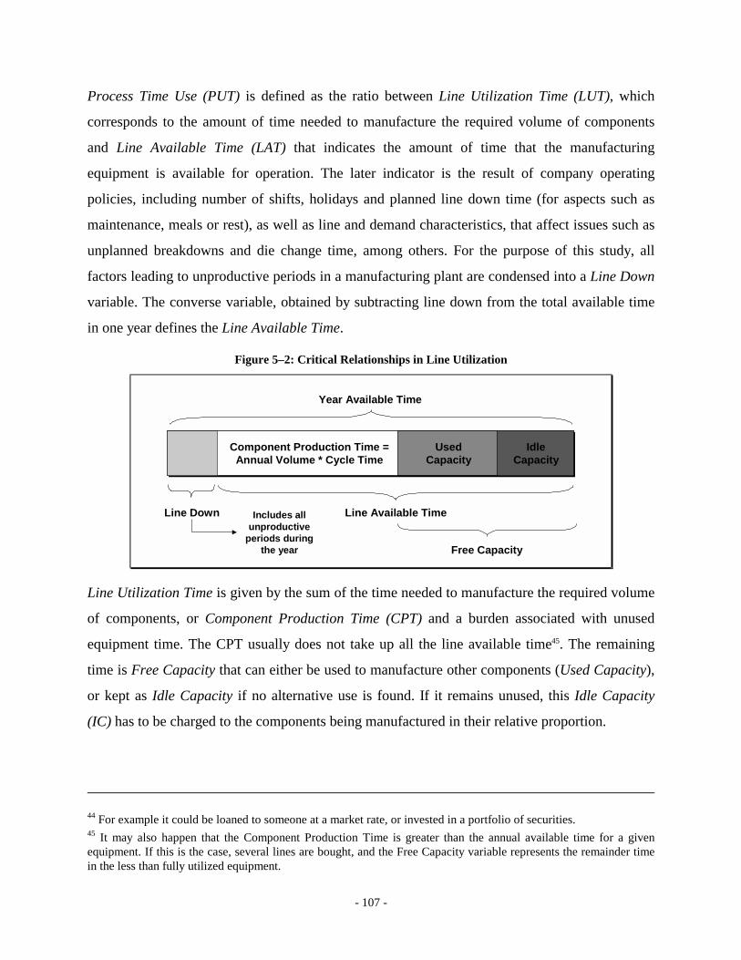
- 107 -

Process Time Use (PUT) is defined as the ratio between Line Utilization Time (LUT), which

corresponds to the amount of time needed to manufacture the required volume of components

and Line Available Time (LAT) that indicates the amount of time that the manufacturing

equipment is available for operation. The later indicator is the result of company operating

policies, including number of shifts, holidays and planned line down time (for aspects such as

maintenance, meals or rest), as well as line and demand characteristics, that affect issues such as

unplanned breakdowns and die change time, among others. For the purpose of this study, all

factors leading to unproductive periods in a manufacturing plant are condensed into a Line Down

variable. The converse variable, obtained by subtracting line down from the total available time

in one year defines the Line Available Time.

Figure 5–2: Critical Relationships in Line Utilization

Year Available Time

Component Production Time =Annual Volume * Cycle Time

Idle Capacity

Line Available TimeLine Down Includes all unproductive

periods during the year

Used Capacity

Free Capacity

Line Utilization Time is given by the sum of the time needed to manufacture the required volume

of components, or Component Production Time (CPT) and a burden associated with unused

equipment time. The CPT usually does not take up all the line available time45. The remaining

time is Free Capacity that can either be used to manufacture other components (Used Capacity),

or kept as Idle Capacity if no alternative use is found. If it remains unused, this Idle Capacity

(IC) has to be charged to the components being manufactured in their relative proportion.

44 For example it could be loaned to someone at a market rate, or invested in a portfolio of securities. 45 It may also happen that the Component Production Time is greater than the annual available time for a given equipment. If this is the case, several lines are bought, and the Free Capacity variable represents the remainder time in the less than fully utilized equipment.

- 108 -

Figure 5–2 illustrates the relationship between these variables. Since CPT can be calculated by

multiplying Cycle Time and Annual Production Volume (Vol), the Unit Fixed Cost (UFC) can be

written as:

(5–1) ( )VolAFC

LATICLATICCTVol

VolAFC

LATLUT

VolAFCPUTUFC )/(1** −+===

AFCICLAT

ICLATCTUFC .1

−+=

The utilization of free capacity is important because it influences the unit cost of the component

under analysis. On the one hand, if free capacity is fully utilized, then idle capacity is zero and

the second term on the right hand side of equation (5–1) drops to zero. As a result, unit cost is

only the relative share of cycle time on the overall production time available in the year. On the

other hand, it is easy to see that if the idle capacity is large, the unit cost will be mostly

determined by the entire line cost and not the individual component production time.

Cycle time and idle time information, together with fixed and variable investment cost

calculations detailed above, provide a rather accurate estimate of the cost associated with an

individual part. Moreover, since calculations are based on engineering estimates, it is possible to

understand how variation in the characteristics of the part may affect manufacturing cost.

5.2.4. Technical Cost Modeling Extensions

The previous sections, following the approach of traditional TCM analyses, described the

problem of cost modeling from the perspective of individual processes. In fact, the initial

research that led to the development of TCM aimed at estimating cost implications of adopting

alternative materials in a particular process; or comparing the manufacturing cost of a particular

component when using different processes. Good examples of these two applications are the

investigation of Busch (1987) on the economic impact of using different polymer resins in

injection molding, or the work by Busch and Field (1988) comparing injection molding with

blow molding, thermoforming and structural foam molding for the manufacturing of panels.

- 109 -

Most applications of TCM since its inception follow a pattern similar to the one described in

these two studies: a limited number of parts are modeled in one or more competing individual

processes to understand the economic implications of changes in process or in critical design

parameters (e.g. material, production volume, factor condition) (Clark, Roth et al., 1997).

Nevertheless, the large majority of today’s products are the result of a complex combination of

parts that require numerous operations in their manufacturing as well as a substantial assembly

effort. The seat of an automobile, for example, may require 40 different individual parts and

more than 10 different processes. As a result, there has been a growing demand for the use of

TCM to estimate more complex products (Han, 1994; Kang, 1998; Kirchain, 1999).

Evaluating the cost of complex products using TCM requires the combination of a significant

number of different models. For each of them, part and processing information has to be gathered

and processed. Because of the high level of detail associated with TCM, combining a large

number of technical cost models will require large amounts of information. For the seat example

mentioned above, given that an average model may require the introduction of 25 descriptive

variables (Kirchain, 1999, chapter 2), more than 10,000 variables would have to be accounted

for. This makes the estimation process extremely complex.

The initial problem resulting from an increase in the number of variables is handling the

information. Traditional TCM have been implemented in spreadsheets, with the user responsible

for the introduction of the variables and the establishment of the necessary links to calculate

aggregate cost from individual models and parts. Entering and manipulating large number of

variables in spreadsheets is not only very time consuming and inefficient, but it also very prone

to errors. An obvious solution to this problem is to migrate the models from the spreadsheet

environment into a more sophisticated modeling environment. To address this problem, Kirchain

(1999) developed an application to support the use of TCM in an object-oriented database

environment. The computer tool created a uniform data structure that describes each part in a

system and the procedures that emulate the behavior and interrelationship of those parts. A case

study of the automobile recycling infrastructure was used to demonstrate the applicability of the

tool.

- 110 -

As in many other problems, the use of computer tools facilitates the TCM problem associated

with manipulating and processing large amounts of information. Nevertheless, as the complexity

of the product to be modeled increases, the problem is not only data manipulation, but also data

collection. Gathering or constructing detailed design and processing data for a large number of

parts is very difficult. A problem that may exist at the onset is access. As products become

complex, detailed design and processing information required as input to TCM is also likely to

be scattered among various persons and departments in a large organization. Furthermore, the

supply chain may become disperse, with various firms responsible for different components. As a

result, data may be very difficult to gather. In addition, even if it would be possible to have all the

required information, inputting and analyzing such a detailed data set can become unmanageable.

For a manufacturing firm, a high level of detail in cost estimation can be very important for

rigorous competitiveness assessment, particularly at the manufacturing stage. If this is the case,

companies assemble large teams of engineering and purchasing people devoted to estimating the

cost of each individual part. Automotive is a good example of an industry where this is often the

case. However, for the overall assessment of a system in early stages of development, or to

investigate the generic impact of changes in factor conditions, such a level of detail is not

desirable or sometimes even possible to achieve. In addition, such a large effort is impossible to

replicate in an academic environment. Therefore, it is important to find methods to approximate

the estimations. At one extreme it is possible to go back to techniques based on rules of thumb.

However, it is reasonable to expect that solutions that reduce data requirements without

compromising the logic and the mechanisms underlying TCM are possible to find.

A potential approach to this problem is the extrapolative method, proposed by Han (1994) and

developed by Kang (1998), to estimate the cost of the body-in-white (BIW) of an automobile.

Instead of modeling approximately 150 parts existing in a BIW, a set of categories were

determined and a representative part to be modeled in detail through TCM was chosen for each

category. The categories were determined according to differences in part geometry, size and

forming complexity. The rest of the parts in the BIW were assigned to each of the categories.

Assuming that all parts were formed in a similar fashion, their cost was estimated using weight

- 111 -

ratios and identical processing conditions to those used for the representative part in each

category.

The two applications show that the extrapolative method can be extremely useful when the parts

have similar processing conditions and common characteristics that can be used to establish the

relative differences. The method may not be so accurate if processing technologies and

conditions are very diverse. A good example of this situation is the attempt to model the whole

3000 components of a car. Unlike the BIW, there is little common ground between components

except the fact that they are all manufactured according to a number of processes. While the BIW

uses only stamping and welding, the 3000 parts of the car require over 20 processes. The

approach for these more complex cases may be still to model all the components, but to reduce

the requirements in terms of the information and the modeling detail associated with each

component. This is approach of the systems cost modeling methodology described in the next

section.

5.3. Systems Cost Modeling (SCM): Estimating the manufacturing cost of

complex systems

The SCM method aims at establishing a systematic way to estimate cost functions for complex

systems, such as the interior or the chassis of a car, where multiple processes and diverse

components are present. The cost function is grounded in engineering based approximate

estimates of the manufacturing and assembly cost of its individual components, aggregated over

subsystems. Unlike most existing cost estimation methods, that aim at obtaining an accurate

evaluation of the manufacturing cost at an individual component level, SCM focuses on

providing reliable calculations of the overall system cost and the influence of key parameters

(such as volume and factor input costs), on the cost behavior.

When comparing manufacturing costs at the individual component level, accuracy and detail in

the estimates is crucial for the relevance of a particular methodology. This is precisely the

objective of TCM. SCM reduces the information intensity when compared to TCM, but it also

provides less precision in cost estimates. Therefore, although SCM provides individual

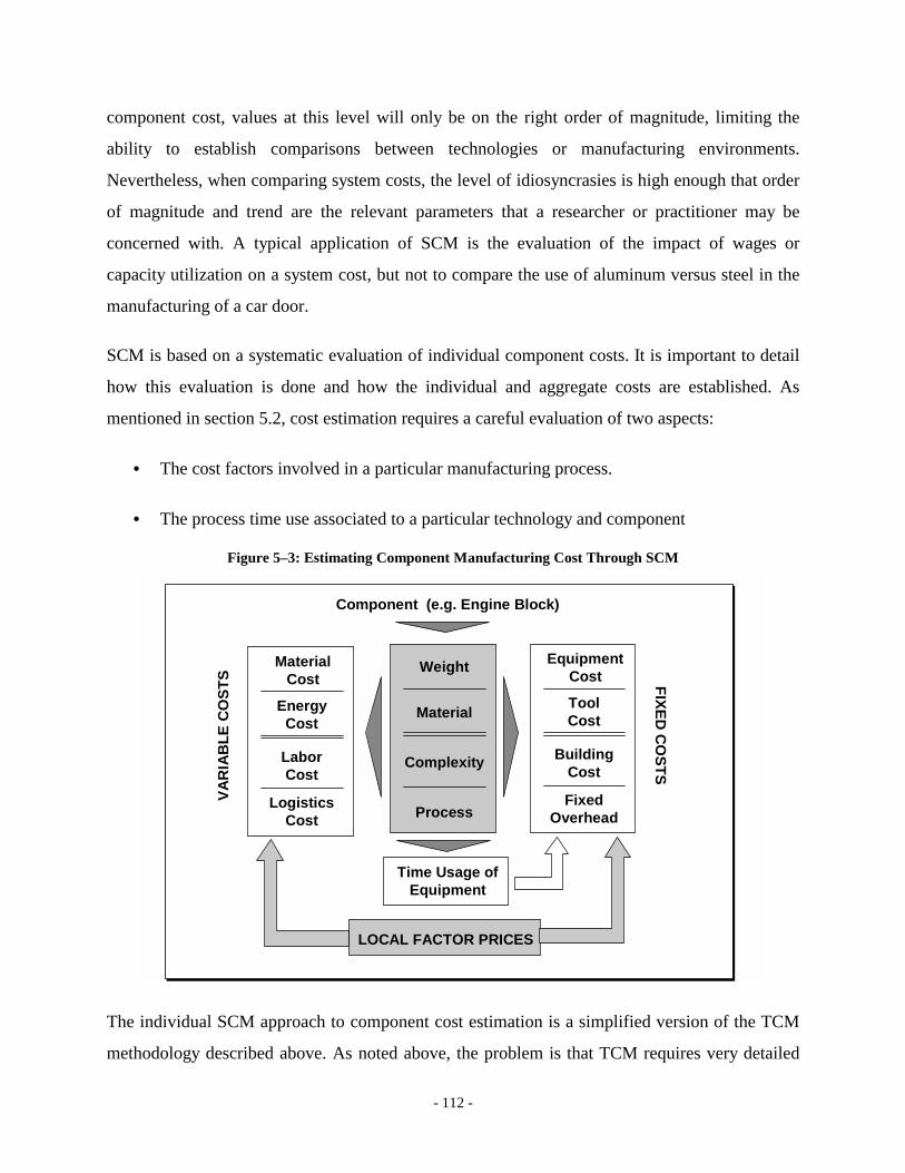
- 112 -

component cost, values at this level will only be on the right order of magnitude, limiting the

ability to establish comparisons between technologies or manufacturing environments.

Nevertheless, when comparing system costs, the level of idiosyncrasies is high enough that order

of magnitude and trend are the relevant parameters that a researcher or practitioner may be

concerned with. A typical application of SCM is the evaluation of the impact of wages or

capacity utilization on a system cost, but not to compare the use of aluminum versus steel in the

manufacturing of a car door.

SCM is based on a systematic evaluation of individual component costs. It is important to detail

how this evaluation is done and how the individual and aggregate costs are established. As

mentioned in section 5.2, cost estimation requires a careful evaluation of two aspects:

• The cost factors involved in a particular manufacturing process.

• The process time use associated to a particular technology and component

Figure 5–3: Estimating Component Manufacturing Cost Through SCM

Weight

Complexity

Component (e.g. Engine Block)

Material

Process

EquipmentCost

BuildingCost

ToolCost

Fixed Overhead

MaterialCost

LaborCost

EnergyCost

Logistics Cost

Time Usage of Equipment

VAR

IAB

LE C

OST

S FIXED COSTS

LOCAL FACTOR PRICES

The individual SCM approach to component cost estimation is a simplified version of the TCM

methodology described above. As noted above, the problem is that TCM requires very detailed

- 113 -

information regarding individual characteristics of the component and associated processing

technology. Therefore, they are particularly useful when comparing designs or material solutions

for individual or small groups of components. But they become less practical and sometimes

infeasible when trying to model several hundred components. SCM solves that problem by

estimating each of cost factors and process use time with limited information and using simple

rules. The level of data detail is reduced, but cost estimates are also less precise.

The critical SCM approach to simplify traditional technical cost modeling techniques, illustrated

in Figure 5–3, is to use four simple metrics as the basis for establishing all the cost drivers of an

individual part. The metrics considered in the analysis are:

• Weight. This indicator is readily available for any component, making it a very natural

choice. It’s important for the material cost estimate and serves as a proxy for the volume of

the component, often a major factor determining the characteristics of the required processing

equipment and tooling.

• Material. Information is usually directly available for each component, even when several

materials are a mixed together. Moreover, it is critical to estimate the material cost, which is

often a significant portion of the total.

• Complexity. Detailed information regarding shape, thickness and other factors used to

calculate equipment characteristics are substituted by a three level complexity factor,

estimated by judgment. Level 1 corresponds to simple components where their size is the

major factor affecting processing; higher levels of complexity imply more detail or additional

features that require more complex (and therefore more expensive) equipment.

An example is a convoluted injection molded part, which would require (a) a more complex

and therefore more expensive tool; (b) higher pressures to cope with the complex mold that

result in a larger more costly machine; (c) longer times to fill the cavity, affecting time

utilization of equipment as well as labor; (d) greater scrap losses due to engineering trim or

rejects.

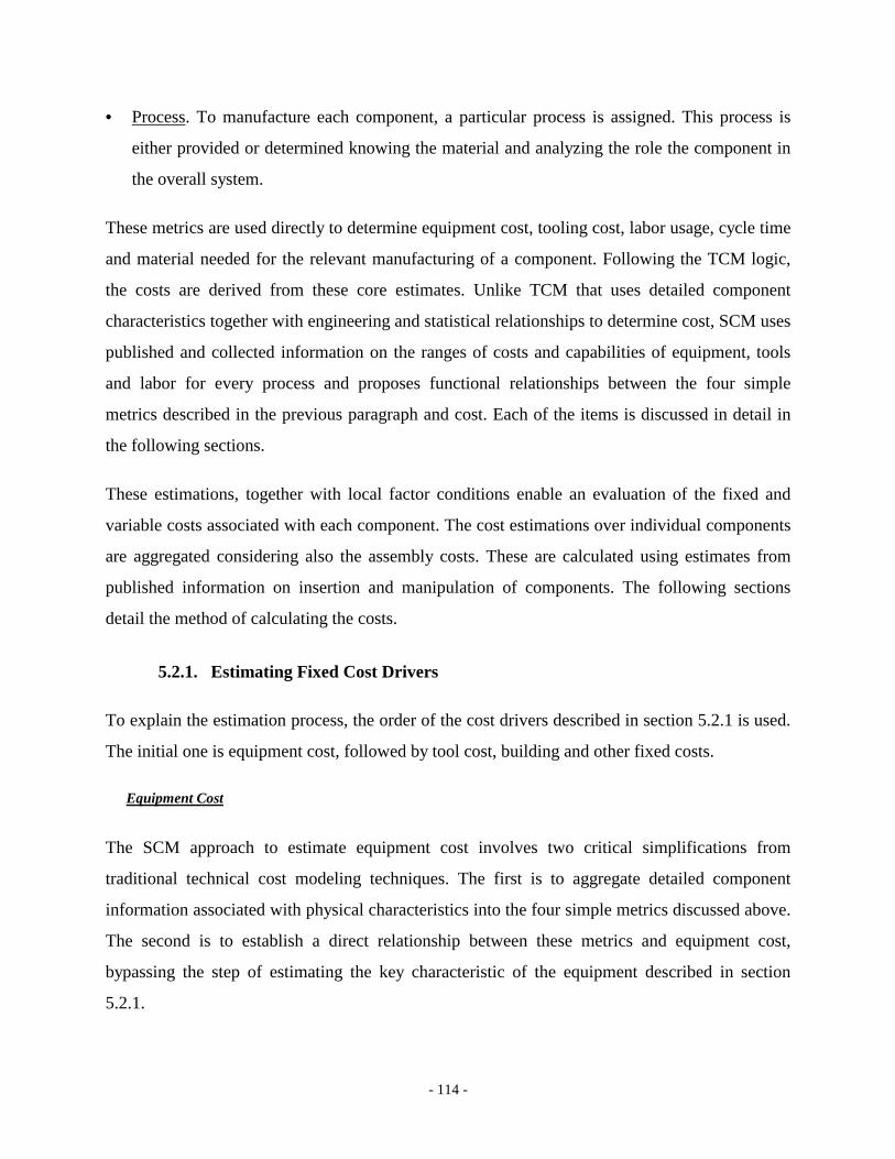
- 114 -

• Process. To manufacture each component, a particular process is assigned. This process is

either provided or determined knowing the material and analyzing the role the component in

the overall system.

These metrics are used directly to determine equipment cost, tooling cost, labor usage, cycle time

and material needed for the relevant manufacturing of a component. Following the TCM logic,

the costs are derived from these core estimates. Unlike TCM that uses detailed component

characteristics together with engineering and statistical relationships to determine cost, SCM uses

published and collected information on the ranges of costs and capabilities of equipment, tools

and labor for every process and proposes functional relationships between the four simple

metrics described in the previous paragraph and cost. Each of the items is discussed in detail in

the following sections.

These estimations, together with local factor conditions enable an evaluation of the fixed and

variable costs associated with each component. The cost estimations over individual components

are aggregated considering also the assembly costs. These are calculated using estimates from

published information on insertion and manipulation of components. The following sections

detail the method of calculating the costs.

5.2.1. Estimating Fixed Cost Drivers

To explain the estimation process, the order of the cost drivers described in section 5.2.1 is used.

The initial one is equipment cost, followed by tool cost, building and other fixed costs.

Equipment Cost

The SCM approach to estimate equipment cost involves two critical simplifications from

traditional technical cost modeling techniques. The first is to aggregate detailed component

information associated with physical characteristics into the four simple metrics discussed above.

The second is to establish a direct relationship between these metrics and equipment cost,

bypassing the step of estimating the key characteristic of the equipment described in section

5.2.1.

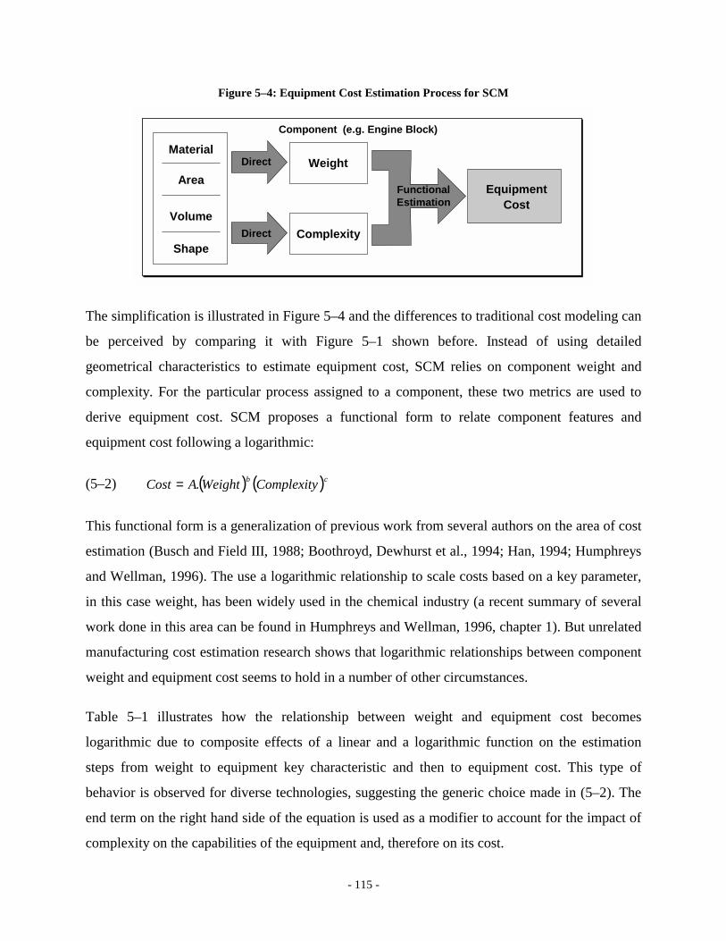
- 115 -

Figure 5–4: Equipment Cost Estimation Process for SCM

Component (e.g. Engine Block)

Material

Volume

Area

Shape

EquipmentCost

Weight

Complexity

FunctionalEstimation

Direct

Direct

The simplification is illustrated in Figure 5–4 and the differences to traditional cost modeling can

be perceived by comparing it with Figure 5–1 shown before. Instead of using detailed

geometrical characteristics to estimate equipment cost, SCM relies on component weight and

complexity. For the particular process assigned to a component, these two metrics are used to

derive equipment cost. SCM proposes a functional form to relate component features and

equipment cost following a logarithmic:

(5–2) ( ) ( )cb ComplexityWeightACost .=

This functional form is a generalization of previous work from several authors on the area of cost

estimation (Busch and Field III, 1988; Boothroyd, Dewhurst et al., 1994; Han, 1994; Humphreys

and Wellman, 1996). The use a logarithmic relationship to scale costs based on a key parameter,

in this case weight, has been widely used in the chemical industry (a recent summary of several

work done in this area can be found in Humphreys and Wellman, 1996, chapter 1). But unrelated

manufacturing cost estimation research shows that logarithmic relationships between component

weight and equipment cost seems to hold in a number of other circumstances.

Table 5–1 illustrates how the relationship between weight and equipment cost becomes

logarithmic due to composite effects of a linear and a logarithmic function on the estimation

steps from weight to equipment key characteristic and then to equipment cost. This type of

behavior is observed for diverse technologies, suggesting the generic choice made in (5–2). The

end term on the right hand side of the equation is used as a modifier to account for the impact of

complexity on the capabilities of the equipment and, therefore on its cost.

- 116 -

Table 5–1: Generic Functional Relationship Between Weight, Equipment Key Characteristic and Cost

Process Weight Key Charact Eq. Cost Source

Injec. Molding Logarithmic Clamp Force Linear (1)

Die Casting Logarithmic Clamp Force Linear (2)

Stamping Linear Press Force Logarithmic (3)

Machining Linear to Logarithmic (4) Sources: Own calculations based on (1) Boothroyd, 1994, Chapter 8; (2) Chapter 10; (4) Chapter 7; (3) Han, 1994.

Assuming that the relationship proposed in equation (5–2) holds, the relevant parameters A, b

and c have to be estimated. Following previous examples, an obvious estimation method would

be to perform regressions of observed equipment cost on the relevant parameters for a number of

parts and processes. Unfortunately, given the pioneer stage of the method, data for such

estimation is still not available. Therefore, the choice was to have an initial estimate of the three

coefficients in the proposed relationship based on a three-point estimation.

While any three points can be used, the particular evaluation that was selected follows the

procedure described below:

1. Identification of extreme points. The choices for two of the points were the extremes. For a

range of components for which equipment cost is to be estimated, the extreme points are such

that the component with minimum weight (Min_Weight) and complexity equal to one is

associated with the minimum equipment cost (Min_Cost), and the component with maximum

weight (Max_Weight) and complexity level equal to three corresponds to the highest

equipment cost (Max_Cost). This uses the weight and complexity information for the set of

parts manufactured with the relevant technology. Equipment costs for the extreme parts is

gathered either from published sources or directly from equipment suppliers.

2. Mid point estimation. An additional point is required to complete the estimation. The strategy

was to choose a point that would define the relative importance of complexity and weight in

establishing equipment cost. The mid point chosen corresponds to a simple part (complexity

equal to one) with maximum weight defines the share of the maximum equipment cost that is

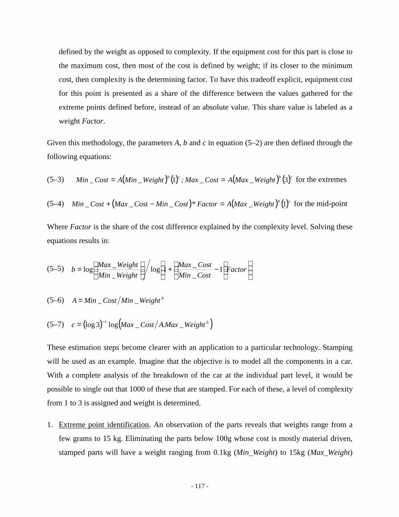
- 117 -

defined by the weight as opposed to complexity. If the equipment cost for this part is close to

the maximum cost, then most of the cost is defined by weight; if its closer to the minimum

cost, then complexity is the determining factor. To have this tradeoff explicit, equipment cost

for this point is presented as a share of the difference between the values gathered for the

extreme points defined before, instead of an absolute value. This share value is labeled as a

weight Factor.

Given this methodology, the parameters A, b and c in equation (5–2) are then defined through the

following equations:

(5–3) ( ) ( ) ( ) ( )cbcb WeightMaxACostMax ;WeightMinACostMin 3__1__ == for the extremes

(5–4) ( ) ( ) ( )cbWeightMaxAFactorCostMinCostMaxCostMin 1_*___ =−+ for the mid-point

Where Factor is the share of the cost difference explained by the complexity level. Solving these

equations results in:

(5–5)

−+

= Factor

CostMinCostMax

WeightMinWeightMaxb 1

__1log

__log

(5–6) bWeightMinCostMinA __=

(5–7) ( ) ( )bWeightMaxACostMaxc _._log3log 1−=

These estimation steps become clearer with an application to a particular technology. Stamping

will be used as an example. Imagine that the objective is to model all the components in a car.

With a complete analysis of the breakdown of the car at the individual part level, it would be

possible to single out that 1000 of these that are stamped. For each of these, a level of complexity

from 1 to 3 is assigned and weight is determined.

1. Extreme point identification. An observation of the parts reveals that weights range from a

few grams to 15 kg. Eliminating the parts below 100g whose cost is mostly material driven,

stamped parts will have a weight ranging from 0.1kg (Min_Weight) to 15kg (Max_Weight)

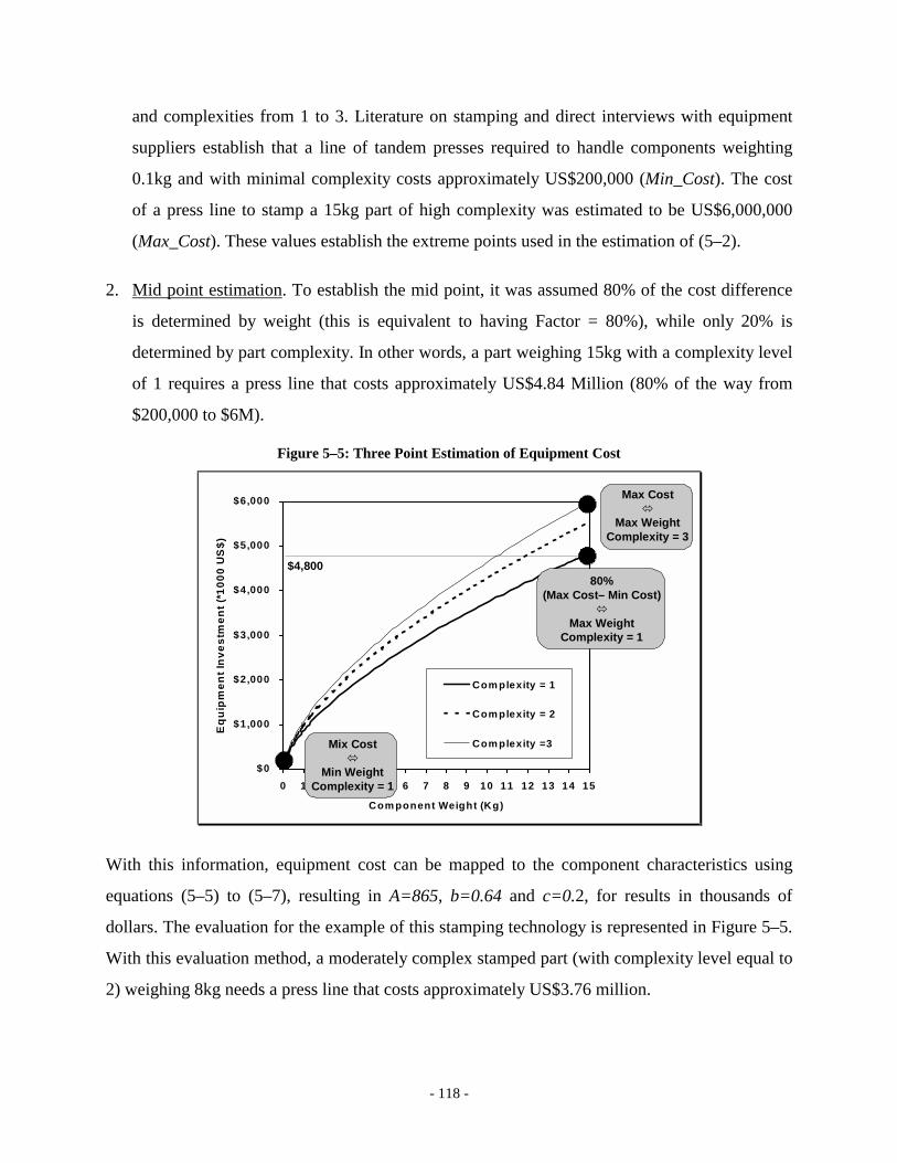
- 118 -

and complexities from 1 to 3. Literature on stamping and direct interviews with equipment

suppliers establish that a line of tandem presses required to handle components weighting

0.1kg and with minimal complexity costs approximately US$200,000 (Min_Cost). The cost

of a press line to stamp a 15kg part of high complexity was estimated to be US$6,000,000

(Max_Cost). These values establish the extreme points used in the estimation of (5–2).

2. Mid point estimation. To establish the mid point, it was assumed 80% of the cost difference

is determined by weight (this is equivalent to having Factor = 80%), while only 20% is

determined by part complexity. In other words, a part weighing 15kg with a complexity level

of 1 requires a press line that costs approximately US$4.84 Million (80% of the way from

$200,000 to $6M).

Figure 5–5: Three Point Estimation of Equipment Cost

$0

$1,000

$2,000

$3,000

$4,000

$5,000

$6,000

0 1 2 3 4 5 6 7 8 9 10 11 12 13 14 15

Com ponent Weight (Kg)

Equ

ipm

ent I

nves

tmen

t (*1

000

US

$)

Com plexity = 1

Com plexity = 2

Com plexity =3

Max Cost !

Max WeightComplexity = 3

80% (Max Cost– Min Cost)

!Max Weight

Complexity = 1

Mix Cost !

Min WeightComplexity = 1

$4,800

With this information, equipment cost can be mapped to the component characteristics using

equations (5–5) to (5–7), resulting in A=865, b=0.64 and c=0.2, for results in thousands of

dollars. The evaluation for the example of this stamping technology is represented in Figure 5–5.

With this evaluation method, a moderately complex stamped part (with complexity level equal to

2) weighing 8kg needs a press line that costs approximately US$3.76 million.

- 119 -

As explained in section 5.2.1, calculations for the base equipment cost are corrected to account

for auxiliary equipment and installation costs, usually as a percentage of the equipment cost. This

practice will be maintained here . The share of auxiliary equipment cost considered is 25%. For

installation costs the value gathered from industry quotes is 15%. With these values, the 8kg

stamping example would require an additional $940,000 in auxiliary equipment and $564,000 for

installation.

The steps to calculate the base equipment cost and the corrections associated auxiliary equipment

and installation determine the equipment fixed costs represented in Figure 5–3. This process

described in detail for the stamping equipment is then replicated for all other technologies

considered in the analysis. The description of relevant cost ranges and parameter values for all

other technologies is presented in Appendix 9.2.

Tooling Cost

Equipment cost is one of the key cost drivers affecting overall manufacturing cost. The other

major fixed cost in a manufacturing activity is tooling costs. The process used to calculate tool

cost is similar to what was described for equipment cost. Again a logarithmic relationship

between component weight and tool cost of the type presented in equation (5–2) is assumed,

using complexity as a cost modifier. This functional form is reasonable because the major driver

for tool cost is its surface area (Busch, 1987; Boothroyd, Dewhurst et al., 1994) and weight is

directly proportional to the volume. This argument is similar to the one used in the chemical

industry to size cost as a log function of capacity (Humphreys and Wellman, 1996, chapter 1).

The difference is related to the effect of complexity on overall tool cost. Complex components

require the tool to have particular characteristics that can substantially change its cost. In

stamping, for example, a tool with moving parts to accomplish a particular component feature

may cost as much as two times that of a component with similar size but with a simple shape

(Han, 1994). A similar fact happens for casting or injection molding (Busch, 1987). Therefore,

when considering equations (5–3) and (5–4) for estimating tool costs, the Factor value that

determines the relative importance of complexity in the cost will be different, assigning greater

relative importance for complexity.

- 120 -

Figure 5–6: Three Point Estimation of Tool Cost

$0

$250

$500

$750

$1,000

$1,250

$1,500

0 1 2 3 4 5 6 7 8 9 10 11 12 13 14 15

W eight of the com ponent (Kg)

Tool

Inve

stm

ent (

*100

0 U

S$)

Com plexity = 1

Com plexity = 2

Com plexity =3

Max Cost !

Max WeightComplexity = 3

50% (Max Cost– Min Cost)

!Max Weight

Complexity = 1

Min Cost !

Min WeightComplexity = 1

Like before, calculating individual tool costs requires the steps described for the case of

equipment costs: the range of component weights and complexities has to be registered,

information from suppliers on the equivalent range of tool costs has to be collected, and new

three point estimation is performed, with the new values and assumptions regarding the weight

factor value. Given this information, the parameters A, b and c in formula (5–2) can be calculated

from equations (5–5) to (5–7). The visual representation of these calculations for the example of

stamping is presented in Figure 5–6, where the base value for the factor considered in the

estimation is 50%, dividing equally the importance of weight and complexity level. Similar steps

are taken for all other relevant technologies.

Other Fixed Cost

The remaining costs associated with a particular manufacturing technology can be calculated

from equipment and tooling costs:

• Building. Consultation with industry and previous studies has placed building cost as 4% to

8% of equipment cost. The base value considered for the study is 6%.

- 121 -

• Maintenance. Equipment, tools and buildings need to be carefully maintained to assure an

adequate operation in a manufacturing environment. This cost is normally considered to be a

share of the value of the item under consideration. A 10% value was used.

• Overhead. The values assumed were 50% of overhead labor over the direct production labor

cost (detailed below) and 25% equipment cost for fixed overheads.

5.3.1. Variable Costs

One of the major cost drivers in industrial processes is material cost. This cost includes not only

the quantity of material that embodies the final component, but also the material that is scrapped,

mostly as a result of trimming and rejects. The major aspect influencing the levels of scrap rate in

a component is its complexity. Therefore, the approach was to link the level of complexity

associated with each component to a given percentage of material that is scrapped (for each good

unit produced). The values considered are 15%, 30% and 45% for levels of complexity of 1, 2

and 3 respectively. Total material cost involves the weight of each component summed with the

respective share of scrap, both multiplied by unit material cost that was gathered from published

sources. The unit costs for each material considered are presented in Appendix 9.2.

Another important variable cost is labor cost. This cost includes the workers that are needed to

operate the equipment required in the relevant manufacturing process, as well as those that

assemble individual parts and components into systems. The methods for calculating the number

of workers needed for manufacturing and assembly are different.

A logarithmic relationship similar to (5–2) is also used to estimate manufacturing labor costs.

The important difference is that the number of workers and not their cost is written as a function

of component characteristics:

(5–8) ( ) ( )cb ComplexityWeightArkersWoofNumber =__

To understand the difference in the approach it is important to note that the market for equipment

is global, with the same suppliers quoting similar prices regardless of the location of the plant.

This makes it possible to establish the unique relationship between equipment cost and part

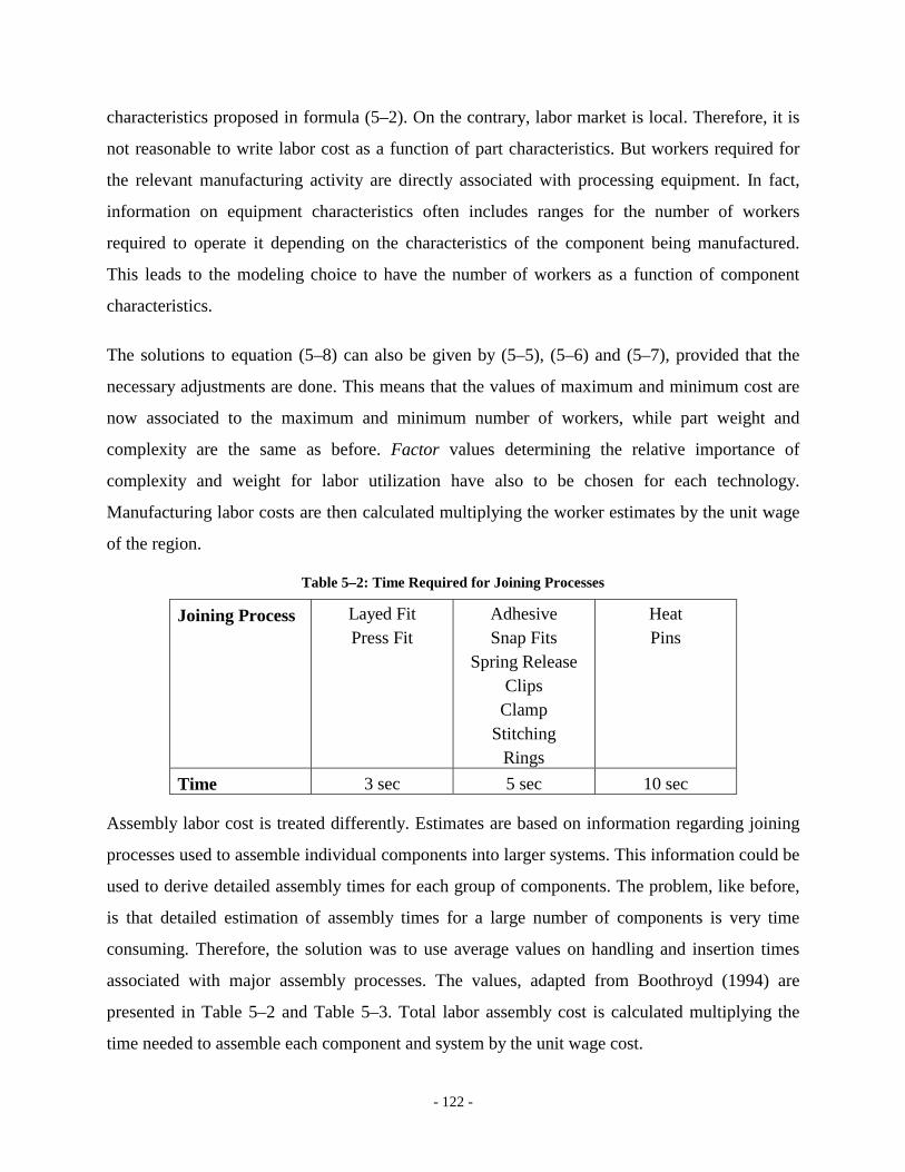
- 122 -

characteristics proposed in formula (5–2). On the contrary, labor market is local. Therefore, it is

not reasonable to write labor cost as a function of part characteristics. But workers required for

the relevant manufacturing activity are directly associated with processing equipment. In fact,

information on equipment characteristics often includes ranges for the number of workers

required to operate it depending on the characteristics of the component being manufactured.

This leads to the modeling choice to have the number of workers as a function of component

characteristics.

The solutions to equation (5–8) can also be given by (5–5), (5–6) and (5–7), provided that the

necessary adjustments are done. This means that the values of maximum and minimum cost are

now associated to the maximum and minimum number of workers, while part weight and

complexity are the same as before. Factor values determining the relative importance of

complexity and weight for labor utilization have also to be chosen for each technology.

Manufacturing labor costs are then calculated multiplying the worker estimates by the unit wage

of the region.

Table 5–2: Time Required for Joining Processes

Joining Process Layed Fit Press Fit

Adhesive Snap Fits

Spring Release Clips

Clamp Stitching

Rings

Heat Pins

Time 3 sec 5 sec 10 sec

Assembly labor cost is treated differently. Estimates are based on information regarding joining

processes used to assemble individual components into larger systems. This information could be

used to derive detailed assembly times for each group of components. The problem, like before,

is that detailed estimation of assembly times for a large number of components is very time

consuming. Therefore, the solution was to use average values on handling and insertion times

associated with major assembly processes. The values, adapted from Boothroyd (1994) are

presented in Table 5–2 and Table 5–3. Total labor assembly cost is calculated multiplying the

time needed to assemble each component and system by the unit wage cost.

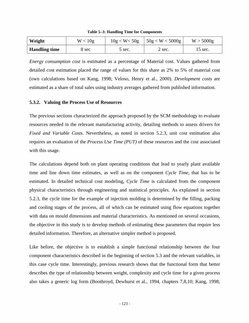
- 123 -

Table 5–3: Handling Time for Components

Weight W < 10g 10g < W< 50g 50g < W < 5000g W > 5000g

Handling time 8 sec 5 sec. 2 sec. 15 sec.

Energy consumption cost is estimated as a percentage of Material cost. Values gathered from

detailed cost estimation placed the range of values for this share as 2% to 5% of material cost

(own calculations based on Kang, 1998; Veloso, Henry et al., 2000). Development costs are

estimated as a share of total sales using industry averages gathered from published information.

5.3.2. Valuing the Process Use of Resources

The previous sections characterized the approach proposed by the SCM methodology to evaluate

resources needed in the relevant manufacturing activity, detailing methods to assess drivers for

Fixed and Variable Costs. Nevertheless, as noted in section 5.2.3, unit cost estimation also

requires an evaluation of the Process Use Time (PUT) of these resources and the cost associated

with this usage.

The calculations depend both on plant operating conditions that lead to yearly plant available

time and line down time estimates, as well as on the component Cycle Time, that has to be

estimated. In detailed technical cost modeling, Cycle Time is calculated from the component

physical characteristics through engineering and statistical principles. As explained in section

5.2.3, the cycle time for the example of injection molding is determined by the filling, packing

and cooling stages of the process, all of which can be estimated using flow equations together

with data on mould dimensions and material characteristics. As mentioned on several occasions,

the objective in this study is to develop methods of estimating these parameters that require less

detailed information. Therefore, an alternative simpler method is proposed.

Like before, the objective is to establish a simple functional relationship between the four

component characteristics described in the beginning of section 5.3 and the relevant variables, in

this case cycle time. Interestingly, previous research shows that the functional form that better

describes the type of relationship between weight, complexity and cycle time for a given process

also takes a generic log form (Boothroyd, Dewhurst et al., 1994, chapters 7,8,10; Kang, 1998;

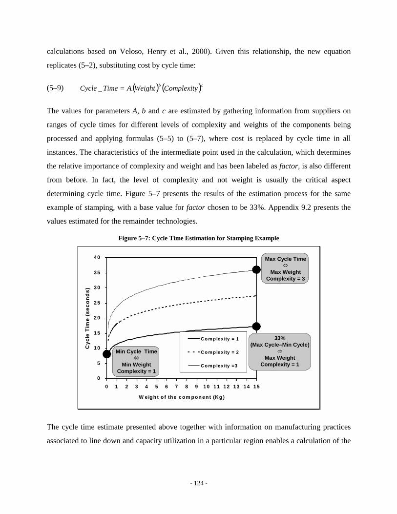
- 124 -

calculations based on Veloso, Henry et al., 2000). Given this relationship, the new equation

replicates (5–2), substituting cost by cycle time:

(5–9) ( ) ( )cb ComplexityWeightATimeCycle ._ =

The values for parameters A, b and c are estimated by gathering information from suppliers on

ranges of cycle times for different levels of complexity and weights of the components being

processed and applying formulas (5–5) to (5–7), where cost is replaced by cycle time in all

instances. The characteristics of the intermediate point used in the calculation, which determines

the relative importance of complexity and weight and has been labeled as factor, is also different

from before. In fact, the level of complexity and not weight is usually the critical aspect

determining cycle time. Figure 5–7 presents the results of the estimation process for the same

example of stamping, with a base value for factor chosen to be 33%. Appendix 9.2 presents the

values estimated for the remainder technologies.

Figure 5–7: Cycle Time Estimation for Stamping Example

0

5

10

15

20

25

30

35

40

0 1 2 3 4 5 6 7 8 9 10 11 12 13 14 15

W eigh t o f the com pon ent (Kg )

Cyc

le T

ime

(sec

onds

)

C om plex ity = 1

C om plexity = 2

C om plexity =3

Max Cycle Time !

Max WeightComplexity = 3

33% (Max Cycle–Min Cycle)

!Max Weight

Complexity = 1

Min Cycle Time!

Min WeightComplexity = 1

The cycle time estimate presented above together with information on manufacturing practices

associated to line down and capacity utilization in a particular region enables a calculation of the

- 125 -

process use time. As explained in equation (5–1), the process use of resources establishes the link

that enables the calculation of the unit fixed costs associated with the manufacturing activities.

5.3.3. Logistics Costs

While most of the cost is driven by the fixed and variable components, logistics may also play an

important role, in particular when considering supply over very large distances. SCM evaluates

logistics cost at two levels. For individual components, an overall baseline logistics cost is

calculated based on published information for the industry as a percentage of the product value.

At the subassembly level, SCM evaluates transportation for the regional shipping scenario under

analysis. First packaging volume and weight for each subassembly is estimated. Second, the

packaging volume is used to calculate all categories contributing to the overall logistics costs.

Packaging volume is the minimum volume needed for the component when being safely

transported. Because information on this measure does not often exist, it is estimated from the

information available on each component through:

(5–10) DensityWeightDFVolumePack /*_ =

As noted before, weight and material data are usually easy to gather for any component. Through

the division between its weight and density, it is possible to have a base estimate of the

component volume if it would be a solid cube. The problem is that components often have odd

shapes that make the packaging volume much greater than this simple calculation. The solution

was to assign each component a Density Factor (DF) that establishes the share of packaging

volume that corresponds to its weight. This information is then used to calculate how many

components can fit in standardized containers that are transported in trucks or boats.

Logistics costs include a number of issues. Those considered for the present study include:

• Packaging cost. The cost of placing components in containers and the cost of the container.

• Truck Cost. This includes procurement, loading and unloading as well as cost per mile.

- 126 -

• Shipping Cost. The whole cost of sending a container on a boat between ports, including

loading and unloading.

• Inventory Cost. The cost associated with the idle components during the transportation

process.

All these costs, except the last, are a function of container or truck size and are gathered from

published information on trucking and shipping transportation sizes, time and cost. Inventory

costs are considered as charge based on the value of the components held in transportation and

the interest rate. For simplicity reasons, the study only considers a direct transportation scenario.

This would be equivalent to having all components and subassemblies delivered to a warehouse

that organizes the Just-In-Time delivery to the OEM.

5.4. Summary

This chapter describes a methodology to evaluate the cost of complex systems with a large

number of individual components and subsystems. This methodology, called Systems Cost

Modeling (SCM) is based on the Technical Cost Modeling technique that has been widely used

to assess manufacturing cost of individual or small groups of components. The problem with

TCM is that when the number of components increases, the amount of information to be

collected and processed rapidly becomes unmanageable.

The SCM approach involves critical simplifications from traditional technical cost modeling

techniques. It proposes simple metrics and rules that enable it to be used to build bottom-up cost

structures for large number of components. Four simple characteristics associated with each

component (weight, process, complexity and material) are inputs to parametric estimates of fixed

and variable costs, as well as process use time of relevant resources. These estimates are then

used to calculate individual component that are then aggregated to the relevant subsystems and

system level.

Unlike most existing cost estimation methods, that aim at obtaining an accurate evaluation of the

manufacturing cost of an individual component level, SCM focuses on providing reliable

- 127 -

calculations of the overall system cost and the influence of key parameters (such as volume and

factor input costs), on the cost behavior. This precisely the objective associated to the domestic

content decision question that the thesis addresses.

- 128 -

Chapter 6. Modeling Cost in the Automotive Supply Chain

The economic models described in chapters 3 and 4 and the cost model presented in chapter 5

can be applied to a number of industries with complex supply chains, ranging from capital goods

to electronics or automotives. Nevertheless, it is important to show whether the issues become

relevant in a particular business and policy environment. The choice was to explore the models in

the context of the automotive industry. This sector has traditionally been one where performance

standards such as domestic content requirements have been present and are still very active.

Moreover the influx of investment in the coming decade towards the developing world is

expected to grow significantly, making this issue more important for governments and firms.

This chapter has two sections. First, it assesses the global trends in the industry and the

purchasing policies in particular. Second it describes the car manufacturing costs in both a

developed and developing region, exploring the tradeoffs and the potential sourcing decisions of

the OEM. These calculations are based on the SCM methodology described in Chapter 5.

6.1. The Automotive Supply Chain

6.1.1. Global Trends in the Auto Industry

One of the major competitive factors is the pattern of demand for new cars. In any of the Triad

regions (Western Europe, Japan and the US) original equipment manufacturers (OEMs) have

been facing a mature market for the past 10 years, with stagnant demand, product proliferation

and stiff price competition. The demand for new cars has been growing on average less than 1%

per year during the past ten years and this trend is forecasted to continue.

A flat demand is aggravated by increased competition in the product market. During the past two

decades, most OEMs have invested heavily in plants outside their home market to better reach

local consumers. As a result, market shares of incumbent players have become thinner. In the

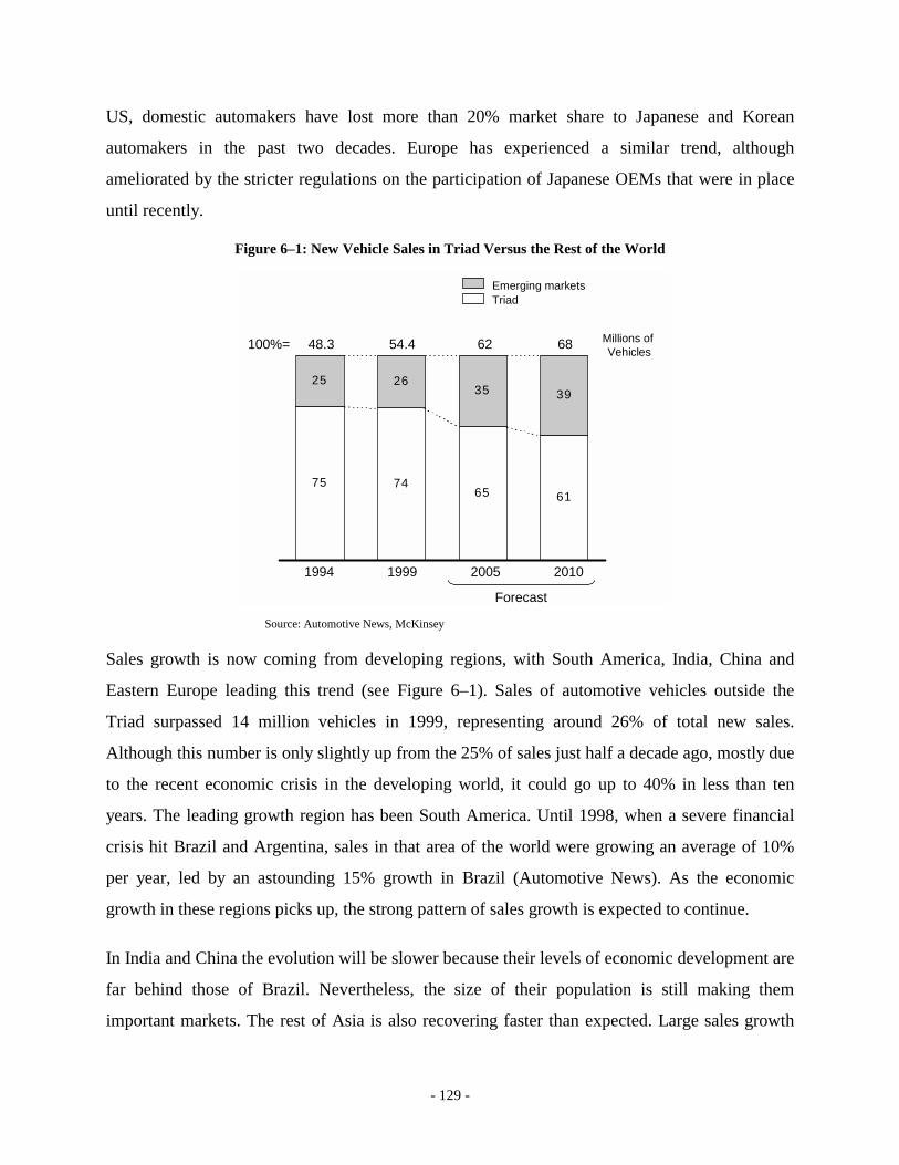
- 129 -

US, domestic automakers have lost more than 20% market share to Japanese and Korean

automakers in the past two decades. Europe has experienced a similar trend, although

ameliorated by the stricter regulations on the participation of Japanese OEMs that were in place

until recently.

Figure 6–1: New Vehicle Sales in Triad Versus the Rest of the World

75 7465 61

25 2635 39

48.3 54.4 62 68100%=

Emerging marketsTriad

Forecast

1994 1999 2005 2010

Millions of Vehicles

Source: Automotive News, McKinsey

Sales growth is now coming from developing regions, with South America, India, China and

Eastern Europe leading this trend (see Figure 6–1). Sales of automotive vehicles outside the

Triad surpassed 14 million vehicles in 1999, representing around 26% of total new sales.

Although this number is only slightly up from the 25% of sales just half a decade ago, mostly due

to the recent economic crisis in the developing world, it could go up to 40% in less than ten

years. The leading growth region has been South America. Until 1998, when a severe financial

crisis hit Brazil and Argentina, sales in that area of the world were growing an average of 10%

per year, led by an astounding 15% growth in Brazil (Automotive News). As the economic

growth in these regions picks up, the strong pattern of sales growth is expected to continue.

In India and China the evolution will be slower because their levels of economic development are

far behind those of Brazil. Nevertheless, the size of their population is still making them

important markets. The rest of Asia is also recovering faster than expected. Large sales growth

- 130 -

forecasted for the ASEAN countries and Korea before the 1997 financial meltdown turned out to

be severe market contractions. Nevertheless, some of these nations recovered rapidly and are now

back to levels of economic growth only slightly below those levels seen before the crisis. As a

result, analysts are reviewing demand estimates monthly, with all the corrections upward.

Another booming area is Eastern Europe. Deprived of car imports during the era of the Soviet

bloc, these nations are using their recent improvements in living standards to buy more cars.

Sales in Eastern Europe (Poland, Hungary, The Czech Republic, Slovakia and Slovenia) reached

one million vehicles, in 1999, double the figure of 1994 (Automotive News).

The evolution of consumer demands, the need to have a global presence and the fast pace of

technological change place important requirements on the participants in the automotive

industry. OEMs have been the players directly affected by these trends. Nevertheless, the

strategies they have pursued as a response to these challenges are having far-reaching effects on

the whole supply chain. The industry is undergoing a period that could be characterized by four

major trends: Globalization, Standardization, Disaggregation and Consolidation.

The first clear characteristic of today’s auto industry is Globalization. Through the end of the

eighties, despite some overseas presence of OEMs, competition was mostly within regional

brands. This picture changed completely during the nineties. A growth of transplants during the

beginning of the decade led to the presence of all competitors in virtually every region (Sturgeon

and Florida, 1999). This has become particularly important in emerging markets, where all

OEMs are fiercely competing for market share as the market grows. As a result, automakers are

now planning operations on a global scale. This means having similar models launched at the

same time in different locations with similar standards.

An intense degree of similarity in the vehicles manufactured across regions has led automakers to

try to replicate successful existing supply chain structures in new locations. This often means

inviting, or sometimes demanding, their suppliers to be present in regions where OEMs are

investing. Suppliers have often seen the OEM globalization trend as an excellent opportunity to

improve their market presence and expand sales volume. As a result, they have followed the

OEMs by expanding into new regions. Nevertheless, suppliers are still far behind any of the

- 131 -

OEMs as true global players. Most of these firms have either total sales or total installed capacity

of less than 50% outside their home markets (Global Interest Group, 1998).

The second critical issue that affects the evolution of the auto industry is standardization.

Declining sales and continuous restyling of models prevent automakers and suppliers alike from

reaching economies of scale in manufacturing, with important adverse impacts on cost. The

solution has been to share components and systems across models and OEMs. This involves the

development of common platforms, the deployment of common processes and the use of

common systems (Lung, Chanaron et al., 1999).

The idea of ‘common platforms’ that homogenize basic structures of the car (like the Golf/A3

VW platform), while allowing adaptations of exterior body is now a prevailing concept among

OEMs. Another important aspect of standardization is the construction of plants able to produce

multiple and varied models, thereby being able to respond to sudden shifts in consumer demands,

or to easily fit in a global capacity management strategy. A similar logic is applied to

components. Suppliers are trying to market systems such as the ABS or the seat frame across car

models and even different OEMs. This possibility could yield important returns, not only due to

scale efficiency, but also because the costs associated with the development of challenging

innovative solutions can be split among several automakers and a much larger number of

manufactured units.

The third aspect that characterizes the industry is value chain disaggregation (Clark and Veloso,

2000). OEMs are focusing their attention on designing and marketing vehicles, as well as

servicing the customer. They wish to reduce the asset intensity of their operations to boost

shareholder return on assets, while improving quality and reducing manufacturing cost. Their

strategy has been to transfer increased responsibilities to existing suppliers and generate

opportunities for the emergence of suppliers with new roles. Part of this transfer of responsibility

involves manufacturing tasks that were previously done by the assembler. The stamping of doors

and fenders are a good example of an activity the OEM has traditionally done, but that is

increasingly being considered for outsourcing. Another dimension of the disaggregation trend is

the divestiture of assemblers from supplier units, which have grown to be full-fledged businesses

- 132 -

of their own. While Visteon and Delphi are the most prominent examples, there are also a myriad

of other smaller players that were spun off from OEMs.

The other industry characteristic, consolidation is directly coupled with the concept of value

chain disaggregation. The need to be present all over the world, the increasing regulatory and

consumer requirements and the need to continuously tackle new technologies, all of this at low

cost, created a tremendous financial pressure on the automakers. As a result, a vast wave of

consolidation is happening among automotive assemblers. It is estimated that, within the next 5

years, less than 10 independent automakers may survive. As OEMs integrate and shed their

involvement in manufacturing, they also concentrate their efforts on working with a smaller

number of players. The new direct suppliers are large global firms, which are either specialized in

complex systems, or integrators of several simpler subsystems. They are expected to have a

substantial responsibility in the design and engineering of these systems and to coordinate the

supply chain necessary for their manufacturing and assembly.

Traditional suppliers were not equipped to respond to this new set of challenges. They were

mostly regional, focusing on particular components, and had limited resources to withstand

financial outlays on product development for up to 3 years before receiving returns on

investment. As a result, during the past few years, the supplier industry has also been undergoing

increasing consolidation. The number of US suppliers with sales between 1 and 5 billion dollars

went from 28 firms in 1992 to 47 companies in 1998. Likewise companies with sales higher than

5 billion dollars increased from 5 to 13 in the same time frame (own calculations from Wards,

several years). The value of merger and acquisition deals peaked at an astounding US$30bn in

1999, representing close to 7% of the total sales of the autoparts industry.

One of most interesting aspects associated with the recent trends in the auto supply chain is the

fact that industry expansion and innovation is happening in emerging regions. OEMs and

suppliers are expanding rapidly in areas like South America, Eastern Europe and Asia, where

they are also trying some of the most innovative solutions in manufacturing and supply chain

organization. For example, the most innovative modular supply approaches, where suppliers

assemble entire modules directly in the OEM plant are happening in Brazil (Lung, Salerno et al.,

1999). This means that, contrary to what has been observed in the past, multinational automotive

- 133 -

companies are trying new solutions outside their core markets. It has also meant that local, often

smaller firms have been active players in new areas of the auto supply chain. A good example of

this situation is the Brazilian steel maker Usiminas. In 1993, Usiminas agreed with Fiat to take

over most of its stamping operations. This agreement is part of a recent OEM trend to increase

the level of outsourcing at the stamping level, an area traditionally done in-house by the OEM.

The interesting aspect is precisely the fact that the early adopter was a local firm rather than a

multinational.

6.1.2. Understanding OEM Purchasing Policies and Decisions

The significant changes that the auto industry is going through influence the purchasing policies

of OEMs and their relationship with the suppliers. The critical issues are the OEM drive towards

increasing supplier responsibility and sourcing practices that are associated with this tendency.

The increase in supplier responsibilities is reaching impressive levels. Renault, for example,

claims that 80% of vehicle value added comes from suppliers (EIU, 1999). Given the increasing

complexity of the systems being subcontracted by the assemblers, there is a clear tendency to

have a smaller number of large suppliers with important responsibilities in the vehicle. For

example, the objective is for Renault to have only 350-400 suppliers by the year 2000 (Veloso,

Henry et al., 2000, chapter 3).

Although there is a general trend towards increasing supplier responsibility and associated

reduction in the number of direct suppliers, assemblers are pursuing different strategies (see

Veloso, Henry et al., 2000 for a comprehensive discussion of these issues). Companies like

Renault and Volkswagen have a more conservative policy strategy in what concerns supplier

reduction, while Ford is being more aggressive. The strategy of VW and Renault could be

described as the 2+1 suppliers. For each subassembly, the assembler forms a strategic partnership

with key suppliers for each region where it is present. Two suppliers are considered privileged

partners, with involvement since the early stages of the development process. A third one will

follow closely, being given less responsibility, but enough for it to be ready to replace any of the

existing suppliers.

- 134 -

Because the same cars are being sold in several regions of the globe, this partnership strategy is

generating a tendency to have also the same suppliers around the world for a given part in a

particular car. Since assemblers demand that car parts have the same characteristics in any given

plant, suppliers often prefer to invest themselves near new the assembly units rather than

transferring process and product knowledge to a local supplier if they don’t follow into new

regions.

The overall Ford-Europe supplier strategy is more radical. The tendency is towards increased use

of entire modules rather than individual components or even subsystems. The ultimate

(theoretical) goal is to have a single source for modules like the entire interior. Most current first

tier suppliers are likely to become second or even third tier and this policy is inevitably going to

lead to a drastic reduction in Ford’s direct supplier count, but might also lead to an overall

reduction in the size of the entire supply chain as consolidation occurs at lower tier levels. As

admitted by Ford, their supply strategy is not the industry standard.

Given what was described above, choosing partners that are able to work with the assemblers in

the development and manufacturing of the systems becomes crucial. Major criteria for the choice

of suppliers include the standard cost and quality competitiveness criteria, and for parts with

substantial logistics costs, location is also an issue. It is also increasingly dependent on R&D

capacity of the first tier suppliers and closeness to the OEM major development centers. It is

clear is that nationality is definitely not a relevant criterion. Another important aspect is that these

first tier suppliers are expected to manage their own supply chain, deciding where they sourcing

the individual components that enter the larger subassemblies that the OEM is buying from them.

Given the degree of requirements and the global presence associated with being a supplier to

these assemblers, how do new firms get accepted as suppliers to the automotive industry? The

typical system is presented in Figure 6–2 (that shows the example of VW) to illustrate how the

process works. The idea is that virtually any supplier with the necessary cost, quality and

development capabilities can be admitted in the supply chain. The admission process is as

follows (Veloso, Henry et al., 2000, Chapter 3):

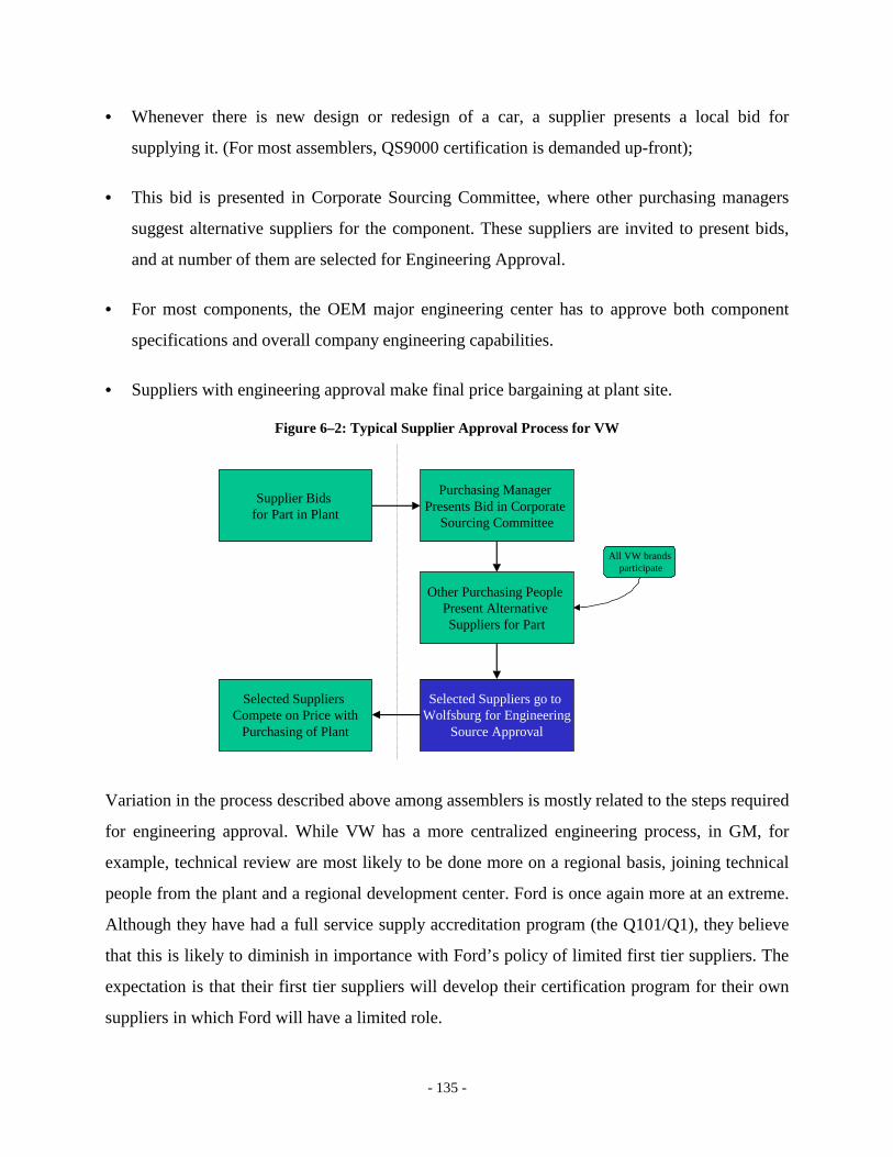
- 135 -

• Whenever there is new design or redesign of a car, a supplier presents a local bid for

supplying it. (For most assemblers, QS9000 certification is demanded up-front);

• This bid is presented in Corporate Sourcing Committee, where other purchasing managers

suggest alternative suppliers for the component. These suppliers are invited to present bids,

and at number of them are selected for Engineering Approval.

• For most components, the OEM major engineering center has to approve both component

specifications and overall company engineering capabilities.

• Suppliers with engineering approval make final price bargaining at plant site.

Figure 6–2: Typical Supplier Approval Process for VW

Supplier Bids for Part in Plant

Purchasing Manager Presents Bid in Corporate

Sourcing Committee

Other Purchasing People Present Alternative Suppliers for Part

Selected Suppliers go to Wolfsburg for Engineering

Source Approval

Selected Suppliers Compete on Price with

Purchasing of Plant

All VW brands participate

Variation in the process described above among assemblers is mostly related to the steps required

for engineering approval. While VW has a more centralized engineering process, in GM, for

example, technical review are most likely to be done more on a regional basis, joining technical

people from the plant and a regional development center. Ford is once again more at an extreme.

Although they have had a full service supply accreditation program (the Q101/Q1), they believe

that this is likely to diminish in importance with Ford’s policy of limited first tier suppliers. The

expectation is that their first tier suppliers will develop their certification program for their own

suppliers in which Ford will have a limited role.

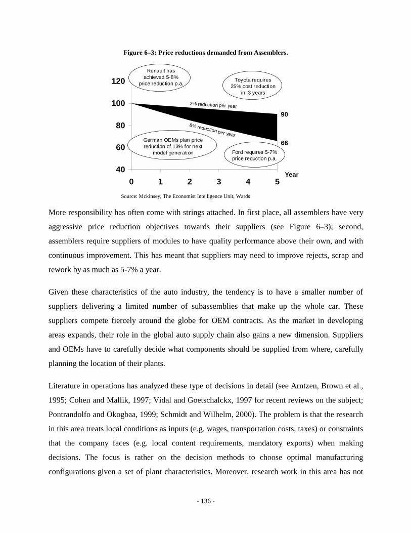
- 136 -

Figure 6–3: Price reductions demanded from Assemblers.

40

60

80

100

120

0 1 2 3 4 5Year

66

90

2% reduction per year

8% reduction per year

Renault has achieved 5-8%

price reduction p.a.Toyota requires

25% cost reduction in 3 years

Ford requires 5-7% price reduction p.a.

German OEMs plan price reduction of 13% for next

model generation

Source: Mckinsey, The Economist Intelligence Unit, Wards

More responsibility has often come with strings attached. In first place, all assemblers have very

aggressive price reduction objectives towards their suppliers (see Figure 6–3); second,

assemblers require suppliers of modules to have quality performance above their own, and with

continuous improvement. This has meant that suppliers may need to improve rejects, scrap and

rework by as much as 5-7% a year.

Given these characteristics of the auto industry, the tendency is to have a smaller number of

suppliers delivering a limited number of subassemblies that make up the whole car. These

suppliers compete fiercely around the globe for OEM contracts. As the market in developing

areas expands, their role in the global auto supply chain also gains a new dimension. Suppliers

and OEMs have to carefully decide what components should be supplied from where, carefully

planning the location of their plants.

Literature in operations has analyzed these type of decisions in detail (see Arntzen, Brown et al.,

1995; Cohen and Mallik, 1997; Vidal and Goetschalckx, 1997 for recent reviews on the subject;

Pontrandolfo and Okogbaa, 1999; Schmidt and Wilhelm, 2000). The problem is that the research

in this area treats local conditions as inputs (e.g. wages, transportation costs, taxes) or constraints

that the company faces (e.g. local content requirements, mandatory exports) when making

decisions. The focus is rather on the decision methods to choose optimal manufacturing

configurations given a set of plant characteristics. Moreover, research work in this area has not

- 137 -

considered the interaction of firm decisions with the social impact on host economies and, in

particular, it has not addressed how may government policy effect firm decisions at a strategic

level. This aspect has been particularly noted in a recent survey of the literature on global

operations, which also referred the shortage of analysis focusing on the realities of developing

nations (Prasad and Sunil, 2000).

The SCM proposed in Chapter 5 and its integration with the models of domestic content

decisions and policies presented in chapters 3 and 4 aims at bridging research on global supply

chain decisions with economic analysis of the implications and drivers of government policies in

developing nations. This is done in the context of an industrial sector that is of growing

importance for these nations. The remainder of this chapter presents an application of SCM to the

automotive supply chain, explaining the characteristics of its cost structure and the influence of

plant location.

6.2. Modeling Automotive Supply Chain Costs

As described in Section 6.1, manufacturing an automobile is an extremely complex and has

strong interdependencies with the regional environment. This is precisely the reason why there

are important interactions between investing OEMs and a multitude of stakeholders, that include

local governments as well as local and global suppliers. These outcomes eventually shape the

supply chain configuration, in particular the origin of the purchased parts and their cost. The

most critical variable shaping the decisions is the cost of the operations, both assembly and

manufacturing. This is the object of this section.

With more than 3000 individual components and as many as 300 sub-assemblies that perform

integrated functions in the vehicle, the car is a clear example of a product for which it becomes

extremely complex to have detailed cost estimations for all the components. In the business

world, automotive companies and their suppliers have large teams of engineers and business

people in charge of costing each sub-assembly during the design and purchasing stages. Despite

this effort, difficult to replicate in the academic environment, information regarding individual

components that compose each sub-assembly is often dispersed along the supply chain, making it

- 138 -

difficult to have accurate estimates from the manufacturers. To be able to evaluate the sourcing

cost structure of a car, the system cost modeling methodology proposed in Chapter 5 is used. As

explained, SCM enables the estimation of manufacturing and logistics costs of systems with

large number of components. Calculations for each component rely on simple metrics that can be

gathered directly from manufactures, estimated by direct observation, or judged from reasonable

criteria.

6.2.1. Unbundling the Car Structure

The cost estimation is based on a comprehensive list of components for a mid-size car of a major

manufacturer46. An extended list, presented in Appendix 9.2, includes the most important of the

3090 individual components, excluding screws, bolts, pins and other small parts. These

individual components are the basis of the system cost modeling estimation. For each of them,

the weight, material, complexity and process information are gathered or attributed. For some,

more than one process is considered47. For example the alternator housing, which is made out of

aluminum, needs first to be die cast and then machined.

Although SCM calculations are performed at the level of individual components, this is not the

relevant level of analysis. As noted before, the objective of the SCM is to enable the evaluation

of cost at the system or subsystem level. Therefore, these levels have to be established for the

object of our evaluations, the car. For this study, individual components are aggregated at two

levels:

• Sourcing. This level clusters components according to sub-assemblies that reflect typical

sourcing decisions for automakers. OEMs have to decide, for example, who will supply the

oil pump, the fuel injection system, or the emergency brake, but not the wires, brackets, cases

and other parts that make these subassemblies. This division yields 274 sub-assemblies, each

with an average of 11 individual components.

46 The brand and model are not revealed for confidentiality reasons 47 SCM considers up to three manufacturing processes per component

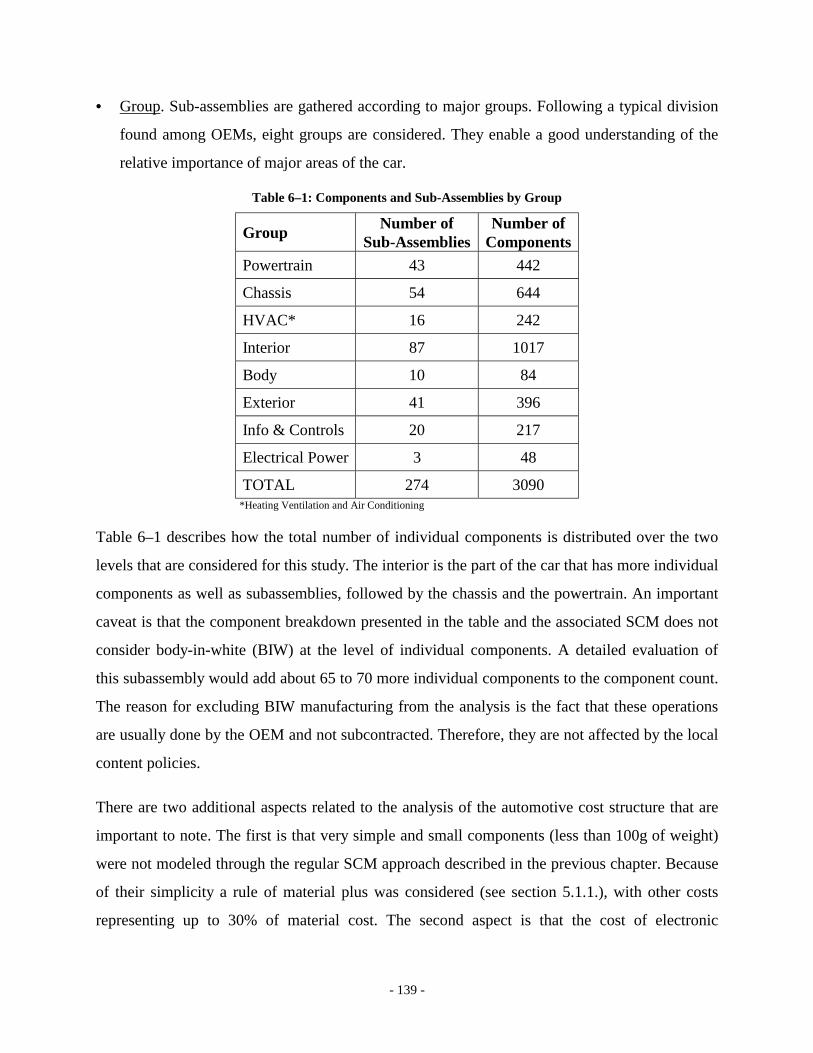
- 139 -

• Group. Sub-assemblies are gathered according to major groups. Following a typical division

found among OEMs, eight groups are considered. They enable a good understanding of the

relative importance of major areas of the car.

Table 6–1: Components and Sub-Assemblies by Group

Group Number of Sub-Assemblies

Number of Components

Powertrain 43 442

Chassis 54 644

HVAC* 16 242

Interior 87 1017

Body 10 84

Exterior 41 396

Info & Controls 20 217

Electrical Power 3 48

TOTAL 274 3090 *Heating Ventilation and Air Conditioning

Table 6–1 describes how the total number of individual components is distributed over the two

levels that are considered for this study. The interior is the part of the car that has more individual

components as well as subassemblies, followed by the chassis and the powertrain. An important

caveat is that the component breakdown presented in the table and the associated SCM does not

consider body-in-white (BIW) at the level of individual components. A detailed evaluation of

this subassembly would add about 65 to 70 more individual components to the component count.

The reason for excluding BIW manufacturing from the analysis is the fact that these operations

are usually done by the OEM and not subcontracted. Therefore, they are not affected by the local

content policies.

There are two additional aspects related to the analysis of the automotive cost structure that are

important to note. The first is that very simple and small components (less than 100g of weight)

were not modeled through the regular SCM approach described in the previous chapter. Because

of their simplicity a rule of material plus was considered (see section 5.1.1.), with other costs

representing up to 30% of material cost. The second aspect is that the cost of electronic

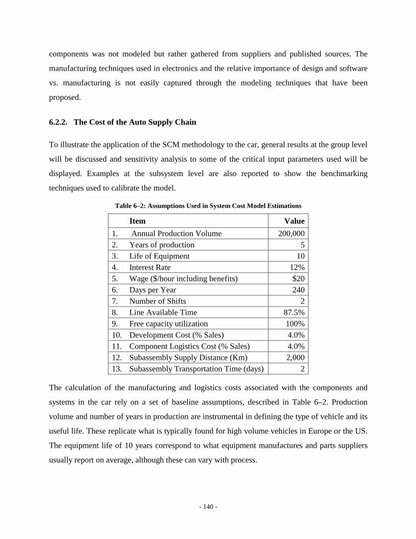
- 140 -

components was not modeled but rather gathered from suppliers and published sources. The

manufacturing techniques used in electronics and the relative importance of design and software

vs. manufacturing is not easily captured through the modeling techniques that have been

proposed.

6.2.2. The Cost of the Auto Supply Chain

To illustrate the application of the SCM methodology to the car, general results at the group level

will be discussed and sensitivity analysis to some of the critical input parameters used will be

displayed. Examples at the subsystem level are also reported to show the benchmarking

techniques used to calibrate the model.

Table 6–2: Assumptions Used in System Cost Model Estimations

Item Value 1. Annual Production Volume 200,000 2. Years of production 5 3. Life of Equipment 10 4. Interest Rate 12% 5. Wage ($/hour including benefits) $20 6. Days per Year 240 7. Number of Shifts 2 8. Line Available Time 87.5% 9. Free capacity utilization 100% 10. Development Cost (% Sales) 4.0% 11. Component Logistics Cost (% Sales) 4.0% 12. Subassembly Supply Distance (Km) 2,000 13. Subassembly Transportation Time (days) 2

The calculation of the manufacturing and logistics costs associated with the components and

systems in the car rely on a set of baseline assumptions, described in Table 6–2. Production

volume and number of years in production are instrumental in defining the type of vehicle and its

useful life. These replicate what is typically found for high volume vehicles in Europe or the US.

The equipment life of 10 years correspond to what equipment manufactures and parts suppliers

usually report on average, although these can vary with process.

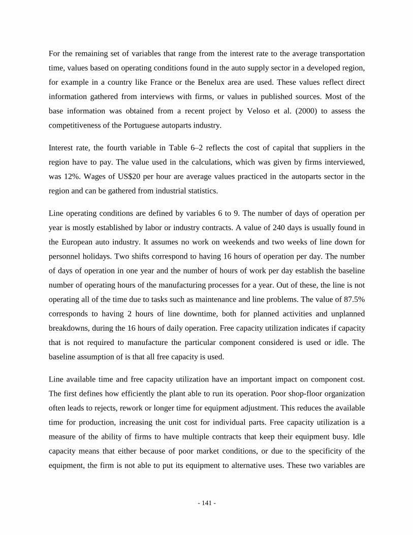
- 141 -

For the remaining set of variables that range from the interest rate to the average transportation

time, values based on operating conditions found in the auto supply sector in a developed region,

for example in a country like France or the Benelux area are used. These values reflect direct

information gathered from interviews with firms, or values in published sources. Most of the

base information was obtained from a recent project by Veloso et al. (2000) to assess the

competitiveness of the Portuguese autoparts industry.

Interest rate, the fourth variable in Table 6–2 reflects the cost of capital that suppliers in the

region have to pay. The value used in the calculations, which was given by firms interviewed,

was 12%. Wages of US$20 per hour are average values practiced in the autoparts sector in the

region and can be gathered from industrial statistics.

Line operating conditions are defined by variables 6 to 9. The number of days of operation per

year is mostly established by labor or industry contracts. A value of 240 days is usually found in

the European auto industry. It assumes no work on weekends and two weeks of line down for

personnel holidays. Two shifts correspond to having 16 hours of operation per day. The number

of days of operation in one year and the number of hours of work per day establish the baseline

number of operating hours of the manufacturing processes for a year. Out of these, the line is not

operating all of the time due to tasks such as maintenance and line problems. The value of 87.5%

corresponds to having 2 hours of line downtime, both for planned activities and unplanned

breakdowns, during the 16 hours of daily operation. Free capacity utilization indicates if capacity

that is not required to manufacture the particular component considered is used or idle. The

baseline assumption of is that all free capacity is used.

Line available time and free capacity utilization have an important impact on component cost.

The first defines how efficiently the plant able to run its operation. Poor shop-floor organization

often leads to rejects, rework or longer time for equipment adjustment. This reduces the available

time for production, increasing the unit cost for individual parts. Free capacity utilization is a

measure of the ability of firms to have multiple contracts that keep their equipment busy. Idle

capacity means that either because of poor market conditions, or due to the specificity of the

equipment, the firm is not able to put its equipment to alternative uses. These two variables are

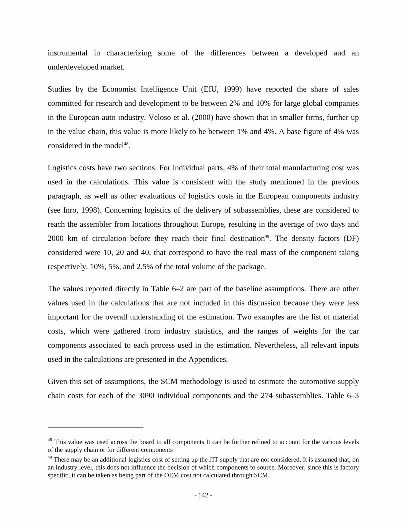
- 142 -

instrumental in characterizing some of the differences between a developed and an

underdeveloped market.

Studies by the Economist Intelligence Unit (EIU, 1999) have reported the share of sales

committed for research and development to be between 2% and 10% for large global companies

in the European auto industry. Veloso et al. (2000) have shown that in smaller firms, further up

in the value chain, this value is more likely to be between 1% and 4%. A base figure of 4% was

considered in the model48.

Logistics costs have two sections. For individual parts, 4% of their total manufacturing cost was

used in the calculations. This value is consistent with the study mentioned in the previous

paragraph, as well as other evaluations of logistics costs in the European components industry

(see Inro, 1998). Concerning logistics of the delivery of subassemblies, these are considered to

reach the assembler from locations throughout Europe, resulting in the average of two days and

2000 km of circulation before they reach their final destination49. The density factors (DF)

considered were 10, 20 and 40, that correspond to have the real mass of the component taking

respectively, 10%, 5%, and 2.5% of the total volume of the package.

The values reported directly in Table 6–2 are part of the baseline assumptions. There are other

values used in the calculations that are not included in this discussion because they were less

important for the overall understanding of the estimation. Two examples are the list of material

costs, which were gathered from industry statistics, and the ranges of weights for the car

components associated to each process used in the estimation. Nevertheless, all relevant inputs

used in the calculations are presented in the Appendices.

Given this set of assumptions, the SCM methodology is used to estimate the automotive supply

chain costs for each of the 3090 individual components and the 274 subassemblies. Table 6–3

48 This value was used across the board to all components It can be further refined to account for the various levels of the supply chain or for different components 49 There may be an additional logistics cost of setting up the JIT supply that are not considered. It is assumed that, on an industry level, this does not influence the decision of which components to source. Moreover, since this is factory specific, it can be taken as being part of the OEM cost not calculated through SCM.

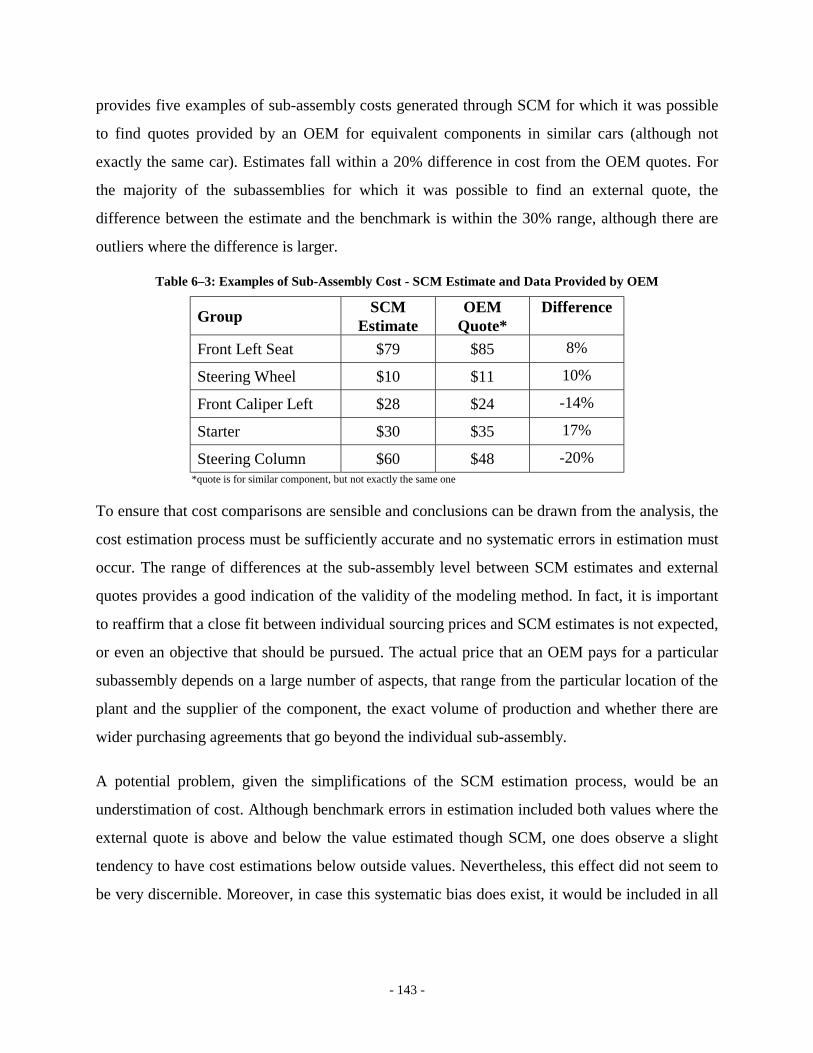
- 143 -

provides five examples of sub-assembly costs generated through SCM for which it was possible

to find quotes provided by an OEM for equivalent components in similar cars (although not

exactly the same car). Estimates fall within a 20% difference in cost from the OEM quotes. For

the majority of the subassemblies for which it was possible to find an external quote, the

difference between the estimate and the benchmark is within the 30% range, although there are

outliers where the difference is larger.

Table 6–3: Examples of Sub-Assembly Cost - SCM Estimate and Data Provided by OEM

Group SCM Estimate

OEM Quote*

Difference

Front Left Seat $79 $85 8%

Steering Wheel $10 $11 10%

Front Caliper Left $28 $24 -14%

Starter $30 $35 17%

Steering Column $60 $48 -20% *quote is for similar component, but not exactly the same one

To ensure that cost comparisons are sensible and conclusions can be drawn from the analysis, the

cost estimation process must be sufficiently accurate and no systematic errors in estimation must

occur. The range of differences at the sub-assembly level between SCM estimates and external

quotes provides a good indication of the validity of the modeling method. In fact, it is important

to reaffirm that a close fit between individual sourcing prices and SCM estimates is not expected,

or even an objective that should be pursued. The actual price that an OEM pays for a particular

subassembly depends on a large number of aspects, that range from the particular location of the

plant and the supplier of the component, the exact volume of production and whether there are

wider purchasing agreements that go beyond the individual sub-assembly.

A potential problem, given the simplifications of the SCM estimation process, would be an

understimation of cost. Although benchmark errors in estimation included both values where the

external quote is above and below the value estimated though SCM, one does observe a slight

tendency to have cost estimations below outside values. Nevertheless, this effect did not seem to

be very discernible. Moreover, in case this systematic bias does exist, it would be included in all

- 144 -

the contexts where costs are estimated and would not favor one of them in particular when

comparisons are required.

The overall results by major area of the car are presented in Figure 6–4. The powertrain is the

most expensive system of a vehicle, followed by the chassis and the interior. The exterior,

HVAC system (Heating Ventilation and Air Conditioning) and body parts make up the second

class of system sourcing cost. The figure also presents an estimate of the engine and body

assembly work to show the relative importance of OEM manufacturing responsibility against

purchased parts. If all the components of the car would be subcontracted, the share of

manufacturing cost that is directly attributed to the OEM is less than 20%. These values also

follow closely the cost estimates that automakers are able to gather from accounting information

for similar vehicles, endorsing the validity of the overall cost estimation process (see Lane, 2000

for public data available on a slightly different aggregation of the major car cost areas).

Figure 6–4: Car Manufacturing Cost

2282

1731

485

1192

507740

510

1,500

8,946BIW ManufacturingEngine Assembly

Powertrain

Chassis

HVACInterior

ExteriorBody

Other

TotalCarMfgCost

Example for mid size vehicle produced in a developed area @ 200,000 units / year

Estimated-Not modeled

$7,446Total Sourcing Cost

Values in US$

Given that SCM analyzes each cost driver and adds them up, it is important to consider how the

overall cost is shared among these drivers. Figure 6–5 presents the sum of all costs across the

automotive component supply chain for each of the included categories. Since SCM only takes

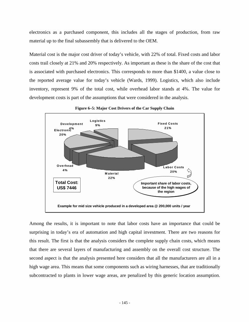
- 145 -

electronics as a purchased component, this includes all the stages of production, from raw

material up to the final subassembly that is delivered to the OEM.

Material cost is the major cost driver of today’s vehicle, with 22% of total. Fixed costs and labor

costs trail closely at 21% and 20% respectively. As important as these is the share of the cost that

is associated with purchased electronics. This corresponds to more than $1400, a value close to

the reported average value for today’s vehicle (Wards, 1999). Logistics, which also include

inventory, represent 9% of the total cost, while overhead labor stands at 4%. The value for

development costs is part of the assumptions that were considered in the analysis.

Figure 6–5: Major Cost Drivers of the Car Supply Chain

Fixed Costs21%

M ateria l22%

O verhead4%

Developm ent4%

Logistics9%

Labor Costs20%

Electron ic20%

Important share of labor costs, because of the high wages of

the region

Total Cost:US$ 7446

Example for mid size vehicle produced in a developed area @ 200,000 units / year

Among the results, it is important to note that labor costs have an importance that could be

surprising in today’s era of automation and high capital investment. There are two reasons for

this result. The first is that the analysis considers the complete supply chain costs, which means

that there are several layers of manufacturing and assembly on the overall cost structure. The

second aspect is that the analysis presented here considers that all the manufacturers are all in a

high wage area. This means that some components such as wiring harnesses, that are traditionally

subcontracted to plants in lower wage areas, are penalized by this generic location assumption.

- 146 -

As it will be shown below, manufacturing in a low wage area may bring this share to values

substantially below the reported 20%.

The results discussed so far are the product of a set of baseline assumptions. Therefore, it is

important to understand how changes in this set of assumptions may alter the values discussed

above. As it can bee seen in Figure 6–6, different items have diverse levels of impact on the

overall cost estimation. Wages, as noted above, have a substantial impact on cost. A reduction of

50% in wage levels results in a decrease in cost of almost $1000, 13% of the total value.

Conversely, an increase in wages from the base value of $20, results in a substantial cost penalty.

Figure 6–6: Sensitivity Analysis of Cost to Main Model Assumptions

$6,500 $7,000 $7,500 $8,000 $8,500 $9,000 $9,500

Volum e

Lin e Av . T im e

Dedicated

W age

Interest Rate

Equip . L ife

Product L ife 8 years – 3 years

15 years – 5 years

8% – 20% / year

$10 – $30 / hour

0% – 100%

95% – 50%

500K – 20K / year

Base Cost: $7, 446

Example for mid size vehicle produced in a developed area @ 200,000 units / year

The two other critical assumptions are production volume and line available time. The first is

intuitive, as less production volume imply the same fixed costs divided by fewer units. While in

what concerns equipment this may not be relevant, provided that the capacity made available can

be used in the production of alternative products, dedicated tooling usually results in a significant

cost penalty at lower production volumes. Line available time is a critical measure of efficiency

in SCM, reflecting the ability of a company to achieve a good utilization of production

equipment. Therefore, it has a significant impact on total cost. Finally, it can be seen from the

- 147 -

influence of the variable ‘dedicated’, i.e. the firm inability to utilize this extra capacity for other

purposes also results in a significant cost penalty. If this equipment is completely dedicated to

manufacturing and assembly of the components under analysis (variable dedicated set to 100%),

overall sourcing cost increases by 10%, roughly $800.

Changes in remaining assumptions have less impact on the overall cost. Interest rates need to

vary significantly to have a meaningful impact on cost. Wide variations are not likely in the

context of a developed region. Nevertheless, if the manufacturing context were to change to a

developing region, often with much higher interest rates, the cost differences could then become

significant. Increases in equipment life do not dramatically change the car sourcing cost, but a

significant decrease in equipment life, due for example to obsolescence of some technologies,

may have an impact.

6.2.3. The impact of Regional Condition on Manufacturing Cost

The sensitivity analysis described in the previous paragraph has shown that the cost structure of

the automotive supply chain is affected by a number of variables, in particular factor costs and

operating conditions. This is an important aspect because the critical idea explored in the thesis is

that of understanding the sourcing decisions of the OEMs in the context of developing nations

and their policies of domestic contents.

The reality in a developing world pushes some of the cost drivers towards higher cost, while

others change in the opposite direction. For example, wages in a developing region are often

much lower than those found in the developed world, contributing to a smaller cost in

manufacturing. On the other hand, the interest rates are higher and the volumes are smaller,

hurting the overall cost. In addition, each of these relevant variables affects individual

components in different ways. A component that is heavily dependent on labor will probably

benefit from the operating conditions of the developing world, while one that has a crucial

dependence on volume may by face important penalties.

Understanding the complete set of conditions and how the affect overall cost is very relevant for

the analysis of local content decisions. Therefore, a new scenario with conditions that are

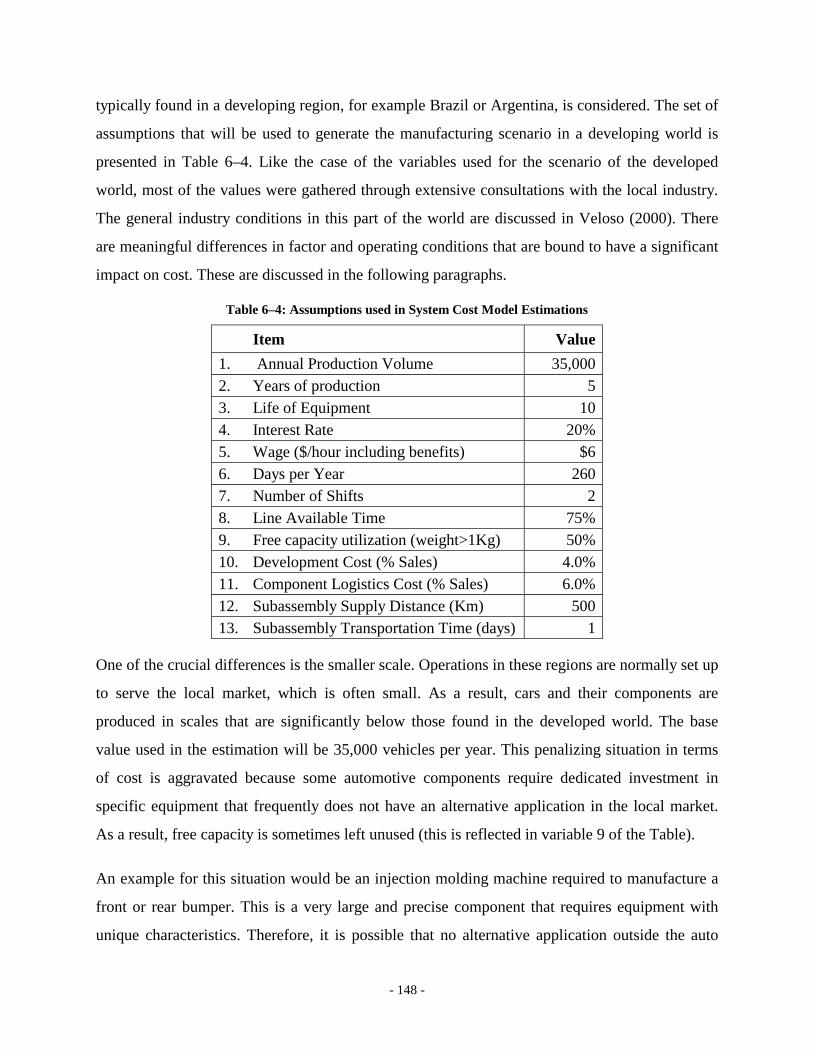
- 148 -

typically found in a developing region, for example Brazil or Argentina, is considered. The set of

assumptions that will be used to generate the manufacturing scenario in a developing world is

presented in Table 6–4. Like the case of the variables used for the scenario of the developed

world, most of the values were gathered through extensive consultations with the local industry.

The general industry conditions in this part of the world are discussed in Veloso (2000). There

are meaningful differences in factor and operating conditions that are bound to have a significant

impact on cost. These are discussed in the following paragraphs.

Table 6–4: Assumptions used in System Cost Model Estimations

Item Value 1. Annual Production Volume 35,000 2. Years of production 5 3. Life of Equipment 10 4. Interest Rate 20% 5. Wage ($/hour including benefits) $6 6. Days per Year 260 7. Number of Shifts 2 8. Line Available Time 75% 9. Free capacity utilization (weight>1Kg) 50% 10. Development Cost (% Sales) 4.0% 11. Component Logistics Cost (% Sales) 6.0% 12. Subassembly Supply Distance (Km) 500 13. Subassembly Transportation Time (days) 1

One of the crucial differences is the smaller scale. Operations in these regions are normally set up

to serve the local market, which is often small. As a result, cars and their components are

produced in scales that are significantly below those found in the developed world. The base

value used in the estimation will be 35,000 vehicles per year. This penalizing situation in terms

of cost is aggravated because some automotive components require dedicated investment in

specific equipment that frequently does not have an alternative application in the local market.

As a result, free capacity is sometimes left unused (this is reflected in variable 9 of the Table).

An example for this situation would be an injection molding machine required to manufacture a

front or rear bumper. This is a very large and precise component that requires equipment with

unique characteristics. Therefore, it is possible that no alternative application outside the auto

- 149 -

industry can be found for such equipment in the context of the developing world. If only small

volumes are required, the equipment may stay idle a substantial part of the time. Nevertheless,

this is not true for all equipment, as simpler parts require equipment that can easily be given

alternative uses. To implement these market characteristics in the SCM estimations, it is assumed

that the equipment used to manufacture components with complexity level equal to 3, or weight

above 1Kg, had 50% of the free capacity not taken by other products. As explained in the

previous section this will imply an additional cost due to greater use time of the equipment.

Another relevant factor related to operating conditions is the efficiency in equipment utilization

(implemented through variable 8 in the Table). Firms in developing regions are less able to

control manufacturing processes, which leads to more unpredicted breakdowns and rework. To

consider this situation, line utilization is reduced to 75% of all potential operating time, down

from 87.5% considered in the developed region. This means that the line is down 2 hours in

every shift of 8, instead of 1 hour considered for the context of the developed world. Because of

the same inefficiency questions, inventory in these firms is also higher than what is found for the

average firm in the western world. The average value gathered from the firms was 6% of sales.

The other crucial difference is in factor conditions. Wages are much lower, and a value of US$6

per hour is considered, consistent with what is found in South America in the industry. With the

contrary behavior of wages, interest rates that determine the opportunity cost of capital are much

higher. The firms interviewed in the industry report this value to be at least 20%, a significant

higher value than found in Europe. This value reflects the scarcity of capital in the region when

compared with the developed worlds, but it also results from unstable macroeconomic conditions

in the region, that often drives interest rates in these regions to high levels. There are more

working days per year, 260 compared with 240 used previously for the developed region, are part

of reported industrial practices.

The average supply distance and time are assumed to be smaller because companies producing

for major OEM manufacturers in these regions are mostly concentrated in the industrial area

where the auto plant is usually located. A good example is the city of S. Paulo which gathers a

substantial share of industrial production of the country.

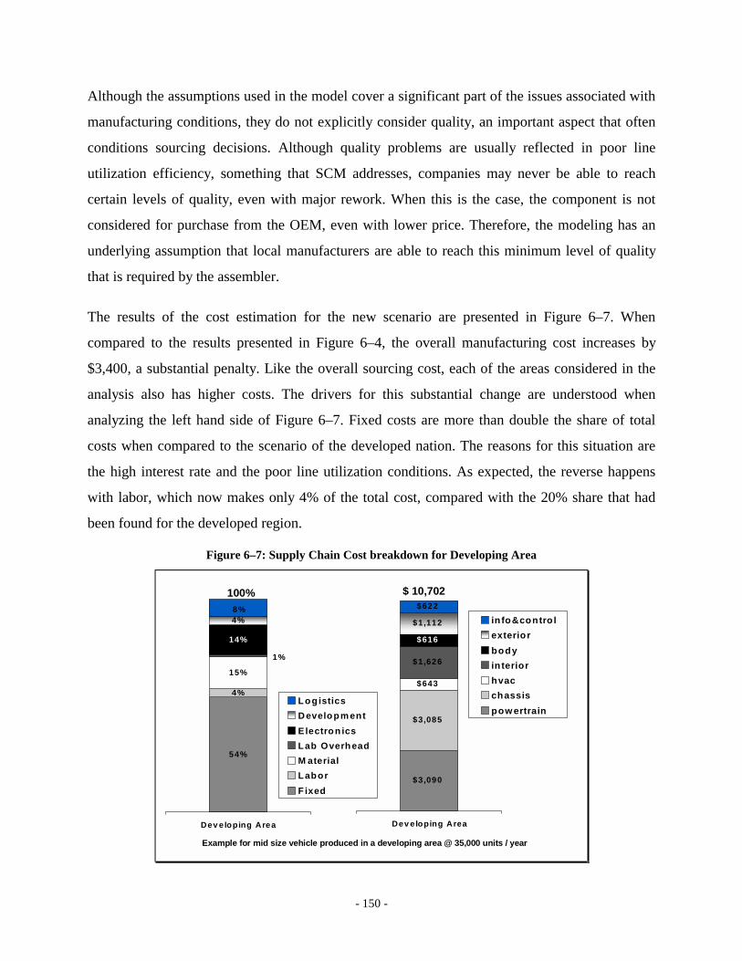
- 150 -

Although the assumptions used in the model cover a significant part of the issues associated with

manufacturing conditions, they do not explicitly consider quality, an important aspect that often

conditions sourcing decisions. Although quality problems are usually reflected in poor line

utilization efficiency, something that SCM addresses, companies may never be able to reach

certain levels of quality, even with major rework. When this is the case, the component is not

considered for purchase from the OEM, even with lower price. Therefore, the modeling has an

underlying assumption that local manufacturers are able to reach this minimum level of quality

that is required by the assembler.

The results of the cost estimation for the new scenario are presented in Figure 6–7. When

compared to the results presented in Figure 6–4, the overall manufacturing cost increases by

$3,400, a substantial penalty. Like the overall sourcing cost, each of the areas considered in the

analysis also has higher costs. The drivers for this substantial change are understood when

analyzing the left hand side of Figure 6–7. Fixed costs are more than double the share of total

costs when compared to the scenario of the developed nation. The reasons for this situation are

the high interest rate and the poor line utilization conditions. As expected, the reverse happens

with labor, which now makes only 4% of the total cost, compared with the 20% share that had

been found for the developed region.

Figure 6–7: Supply Chain Cost breakdown for Developing Area

54%

4%

15%

14%

4%

1%

8%

Dev eloping Area

Log isticsDevelopm entElectron icsLab OverheadM aterialLaborF ixed

$3,090

$3,085

$643

$1,626

$616

$1,112

$622

Dev eloping Area

info&contro lexteriorbodyinteriorhvacchassispow ertrain

$ 10,702

Example for mid size vehicle produced in a developing area @ 35,000 units / year

100%

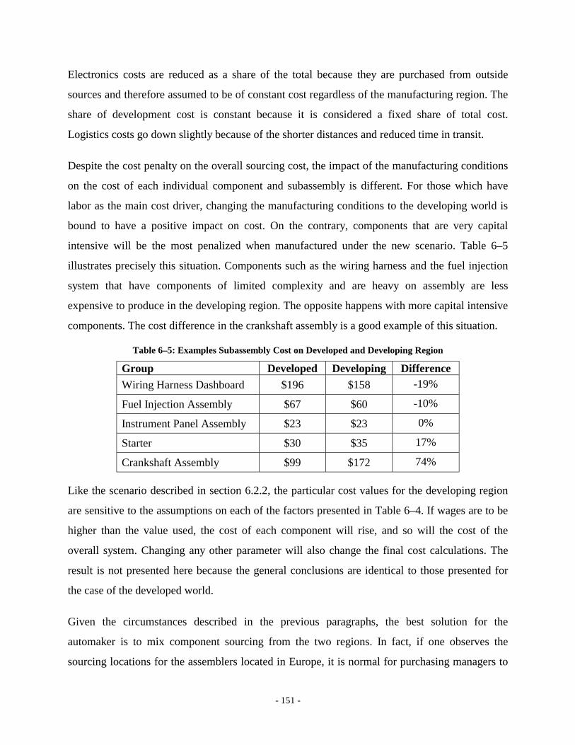
- 151 -

Electronics costs are reduced as a share of the total because they are purchased from outside

sources and therefore assumed to be of constant cost regardless of the manufacturing region. The

share of development cost is constant because it is considered a fixed share of total cost.

Logistics costs go down slightly because of the shorter distances and reduced time in transit.

Despite the cost penalty on the overall sourcing cost, the impact of the manufacturing conditions

on the cost of each individual component and subassembly is different. For those which have

labor as the main cost driver, changing the manufacturing conditions to the developing world is

bound to have a positive impact on cost. On the contrary, components that are very capital

intensive will be the most penalized when manufactured under the new scenario. Table 6–5

illustrates precisely this situation. Components such as the wiring harness and the fuel injection

system that have components of limited complexity and are heavy on assembly are less

expensive to produce in the developing region. The opposite happens with more capital intensive

components. The cost difference in the crankshaft assembly is a good example of this situation.

Table 6–5: Examples Subassembly Cost on Developed and Developing Region

Group Developed Developing Difference Wiring Harness Dashboard $196 $158 -19%

Fuel Injection Assembly $67 $60 -10%

Instrument Panel Assembly $23 $23 0%

Starter $30 $35 17%

Crankshaft Assembly $99 $172 74%

Like the scenario described in section 6.2.2, the particular cost values for the developing region

are sensitive to the assumptions on each of the factors presented in Table 6–4. If wages are to be

higher than the value used, the cost of each component will rise, and so will the cost of the

overall system. Changing any other parameter will also change the final cost calculations. The

result is not presented here because the general conclusions are identical to those presented for

the case of the developed world.

Given the circumstances described in the previous paragraphs, the best solution for the

automaker is to mix component sourcing from the two regions. In fact, if one observes the

sourcing locations for the assemblers located in Europe, it is normal for purchasing managers to

- 152 -

buy components that require significant amounts of labor from the countries in the south or east

of Europe, where wages are lower, and more recently from North African countries. On the

contrary, engine plants and other capital intensive operations often remain in the developed

markets of Germany, France and surrounding nations. How to make this match in the context of

the developing world is the subject of Chapter 7.

6.3. Summary

This chapter explores the System Cost Model described in Chapter 5 in the context of the

automotive industry. First, it assesses the global trends in the industry contrast and the purchasing

policies in particular. Second it describes the car manufacturing costs in both a developed and

developing region, exploring the tradeoffs and the potential sourcing decisions of the OEM.

Data from a particular car is then used build a sourcing cost structure. The cost estimation is

based on a comprehensive list of components for a mid-size car of a major manufacturer,

includes 3090 individual components, excluding screws, bolts, pins or other small parts that are

used in assembly. Individual component costs are estimated and aggregated over 274 major

subassemblies. These constitute the object of sourcing decision of the OEM. The overall results

of the estimation process are presented; critical benchmarks at subsystem and group level and

sensitivity to key parameters are also discussed.

A study comparing the impact of regional conditions is then presented. Calculations show that

overall manufacturing conditions in the developing world have a significant negative impact on

cost. Nevertheless, this effect is not general and depends on the characteristics of individual

components and subsystems. As a result, the best solution for OEMs is to mix component

sourcing from developing and developed regions.

- 153 -

Chapter 7. Domestic Content Requirements and the Auto Supply Chain

This Chapter analyses the specific context of domestic content requirements, integrating the

theoretical models presented in chapters 3 and 4 with the system cost model proposed in chapter

5 and the specific context of the auto industry supply chain presented in chapter 6.

First, it discusses why local content requirements are an important issue in the automotive

industry. The analysis follows the sequence of the models and issues presented in chapters 3 and

4, integrating cost data calculated through the system cost model. In section 7.2, free market

decisions are considered to establish the benchmark sourcing structure against which the various

results will be compared. This calculation provides an understanding of how a domestic content

policy might affect welfare. The implications of potential gaps between social and private costs

of the key resources are investigated and the specific context of learning and spillover effects is

considered. Section 7.3 addresses the situation of optimal contracts and asymmetric information.

In all the analyses, sensitivity to key parameters is examined.

7.1. Domestic Content Policies in the Auto Industry

The automotive industry is a massive generator of economic wealth and employment. In Western

Europe, Japan and the United States, it accounts for as much as 13% of GDP, and one in every

seven people is employed through the industry, either directly or indirectly (i.e. insurance)

(Maxton and Wormald, 1995). Moreover, sectors like rubber or steel are highly dependent on the

50 million cars produced each year. Furthermore, demand characteristics are another critical

aspect of this industry. Buying a car is usually the second largest investment objective of a

family, right after the house. This behavior, that is similar around the world, creates a predictable

need for the availability of cars in every country.

Because of these characteristics, the auto industry has been extremely important to national

economies and a source of concern for the governments, particularly since the 1950s, with a

- 154 -

world 'boom' in the demand for consumer and industrial products (Shapiro, 1993). The late

industrializing countries that started their catch-up process during this period have accrued

sources of concern. As demand started to grow, imports of cars and parts from the world

oligopolistic producers started to create trade balance disparities that affected the capacity to

access capital goods much needed for their industrialization process.

In the process of targeting solutions to address this important issue, most governments realized

that this predictable demand for cars could also be seen as a major industrial development

opportunity. In fact, besides the employment and trade issues, this industry created a significant

demand for intermediate inputs, creating pressure to develop other sectors of the economy. They

figured that the automotive industry could provide a hub for an integrated industrial structure by

triggering the domestic production and technological advance of industries such as steel, machine

tools and components, among others (see for example Krueger, 1975; Amsden, 1989; Shapiro,

1993; Veloso, Soto et al., 1998). The problem was the creation of national industrial capability in

a context of oligopolistic market structures. The solution was the adoption of strong trade

protection mechanisms (quotas, tariffs), forcing assemblers to locate plants in their countries if

they wanted to access local demand. Simultaneously, the enactment of policies to stimulate

Foreign Direct Investment (FDI) and local content requirements would foster the desired linkages

within the national economy. These policies evolved over time and the initial schemes were

complemented later with measures for export promotion, quality, R&D, etc.

The utilization of performance standards to encourage investing firms to reach certain objectives

important for the government and in particular the adoption of domestic content requirements has

been pervasive in the industry. As noted in chapter 2, empirical research suggests that although

with different degrees of success, performance standards played an important role in the

development of the auto industry in countries as diverse as Mexico (Bennet and Sharpe, 1990)

(Veloso, Soto et al., 1998), Taiwan (Veloso, Soto et al., 1998), Portugal (Veloso, Henry et al.,

2000), Korea (Amsden, 1989), Brazil (Shapiro, 1993) and Spain (Lagendijk, 1993), among

others. Among the wide array of policies used to foster the development of the automotive

industry and reported in these and other studies, domestic content has been one of the most

prevalent. Government has considered it a major instrument to promote backward linkages to

- 155 -

local suppliers and encourage the investment of foreign players in the local market, deepening the

supply chain.

Table 7–1: Domestic Content Requirements in Selected Regions

Country or Region Components Local Purchase Policy China 40% to 90% depending on year and product

Malaysia 60% up to 1850cc, 45% up to 2850cc and commercial

Thailand 0% (54% until 2000)

Philippines 40% to 50%

AFTA (Asean Free Trade Area) Expected to be 60%

Mercosur 50% first year, 60% after (new rules under negotiation)

NAFTA 62.5% Rule of Origin; Mexican local requirements until 2004

EU 60% Rule of Origin

India 50% after 3 years, 70% after five years

Korea Non-market barriers: national ownership Sources: www.asean-auto.org (Asean); www.indiainfoline.com (India); www.cacauto.com/ (China);

http://www.rediff.com/ (India); US DOC STAT-USA (rest)

Industrial policies have been tamed by international agreements, in particular the rounds of trade

liberalization that led to the creation of the World Trade Organization. Nevertheless, as detailed

in chapter 2, domestic content requirements have been one of the more resilient government

policies, especially in the auto industry. A number of individual countries still have active

requirements of domestic purchases, aiming to contribute to the development of upstream

industrial capabilities.

Table 7–1 presents the current state of these policies in a number of regions of the world. As it

can be seem, either at the level of individual countries, or within the context of regions, these

regulations continue to be present throughout the globe. Moreover, because of the flexible

conditions of the WTO regarding transition periods, they are bound to continue in the near future.

The persistence and importance of this policy in the context of the automotive industry is the

motivation for choosing it as the case study for the models described in previous chapters that

will be discussed in the next sections.

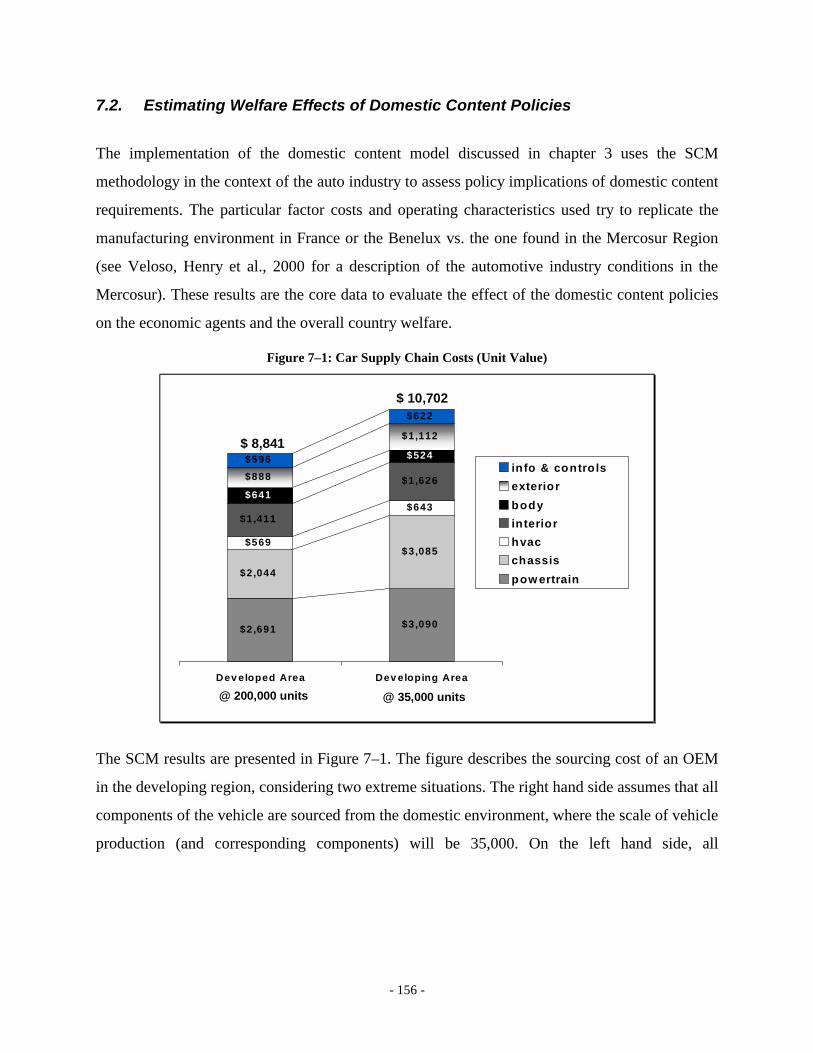
- 156 -

7.2. Estimating Welfare Effects of Domestic Content Policies

The implementation of the domestic content model discussed in chapter 3 uses the SCM

methodology in the context of the auto industry to assess policy implications of domestic content

requirements. The particular factor costs and operating characteristics used try to replicate the

manufacturing environment in France or the Benelux vs. the one found in the Mercosur Region

(see Veloso, Henry et al., 2000 for a description of the automotive industry conditions in the

Mercosur). These results are the core data to evaluate the effect of the domestic content policies

on the economic agents and the overall country welfare.

Figure 7–1: Car Supply Chain Costs (Unit Value)

$2,691 $3,090

$2,044

$3,085$569

$643$1,411

$1,626$641

$524

$888$596

$622

$1,112

Dev eloped Area Dev eloping Area

info & controlsexteriorbodyinteriorhvacchassispow ertrain

$ 10,702

$ 8,841

@ 200,000 units @ 35,000 units

The SCM results are presented in Figure 7–1. The figure describes the sourcing cost of an OEM

in the developing region, considering two extreme situations. The right hand side assumes that all

components of the vehicle are sourced from the domestic environment, where the scale of vehicle

production (and corresponding components) will be 35,000. On the left hand side, all

- 157 -

components are bought from the international market, produced at high production volumes50

(200,000 are assumed) and imported into the country.

The costs for the scenario of manufacturing in the developed world are different from those

presented in chapter 6. The reasons for this difference are the added logistics and duty as well as

tariff costs to which imported components are subject. Logistics costs result from a commercial

freight cost of $1500 associated with shipping a 40’ container for 15 days across the ocean and

an insurance cost of 2% of product value. Duty and tariff costs are 16%, a value established

against what is typically found in South America.

The total sourcing cost in the developing area is higher than the foreign alternative. Nevertheless,

the same does not hold true for all individual subsystems. The body group is less expensive in the

developing world. These aggregate results provide an initial perception of how an automaker

may want to pick and choose suppliers from different regions of the world depending on the

component. If the choices were limited to those described above, an OEM investing in the

developing country would buy the body from local firms and the rest from foreign suppliers.

Using the models developed in chapter 3 and 6, this section analyzes in detail the sourcing

decisions and costs of an automotive OEM, including how these are affected by government

policies, and the overall impact on domestic welfare.

7.2.1. Market Conditions and Sourcing Decisions

To study the pattern of OEM sourcing decisions, the SCM model for the context of the

automotive is used. As described in chapter 6, the decision involves 274 systems that are bought

by the OEM. This almost continuum of components enables a very reasonable replication of the

model described in Chapter 3 regarding OEM sourcing decisions. Figure 7–2 represents an

application of the model to the component data set. The two graphs in the figure show the two

equivalent representations of the problem. On the left hand side, costs are presented as a function

50 The idea is that a similar car is produced in the foreign region, thus taking all the remaining volume of components that is not exported

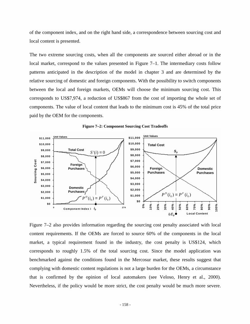
- 158 -

of the component index, and on the right hand side, a correspondence between sourcing cost and

local content is presented.

The two extreme sourcing costs, when all the components are sourced either abroad or in the

local market, correspond to the values presented in Figure 7–1. The intermediary costs follow

patterns anticipated in the description of the model in chapter 3 and are determined by the

relative sourcing of domestic and foreign components. With the possibility to switch components

between the local and foreign markets, OEMs will choose the minimum sourcing cost. This

corresponds to US$7,974, a reduction of US$867 from the cost of importing the whole set of

components. The value of local content that leads to the minimum cost is 45% of the total price

paid by the OEM for the components.

Figure 7–2: Component Sourcing Cost Tradeoffs

$0

$1,000

$2,000

$3,000

$4,000

$5,000

$6,000

$7,000

$8,000

$9,000

$10,000

$11,000

0 274Com ponent Index i

Sou

rcin

g C

ost

Unit Values

Total Cost

Foreign Purchases

Domestic Purchases

i0

)()( 00 iPiP FD =

0)(' =iS

Unit Values

$0

$1,000

$2,000

$3,000

$4,000

$5,000

$6,000

$7,000

$8,000

$9,000

$10,000

$11,000

0% 10%

20%

30%

40%

50%

60%

70%

80%

90%

100%

Local Content

Total Cost

Foreign Purchases

Domestic Purchases

LC0

)()( 00 iPiP FD =

S0

Figure 7–2 also provides information regarding the sourcing cost penalty associated with local

content requirements. If the OEMs are forced to source 60% of the components in the local

market, a typical requirement found in the industry, the cost penalty is US$124, which

corresponds to roughly 1.5% of the total sourcing cost. Since the model application was

benchmarked against the conditions found in the Mercosur market, these results suggest that

complying with domestic content regulations is not a large burden for the OEMs, a circumstance

that is confirmed by the opinion of local automakers (see Veloso, Henry et al., 2000).

Nevertheless, if the policy would be more strict, the cost penalty would be much more severe.

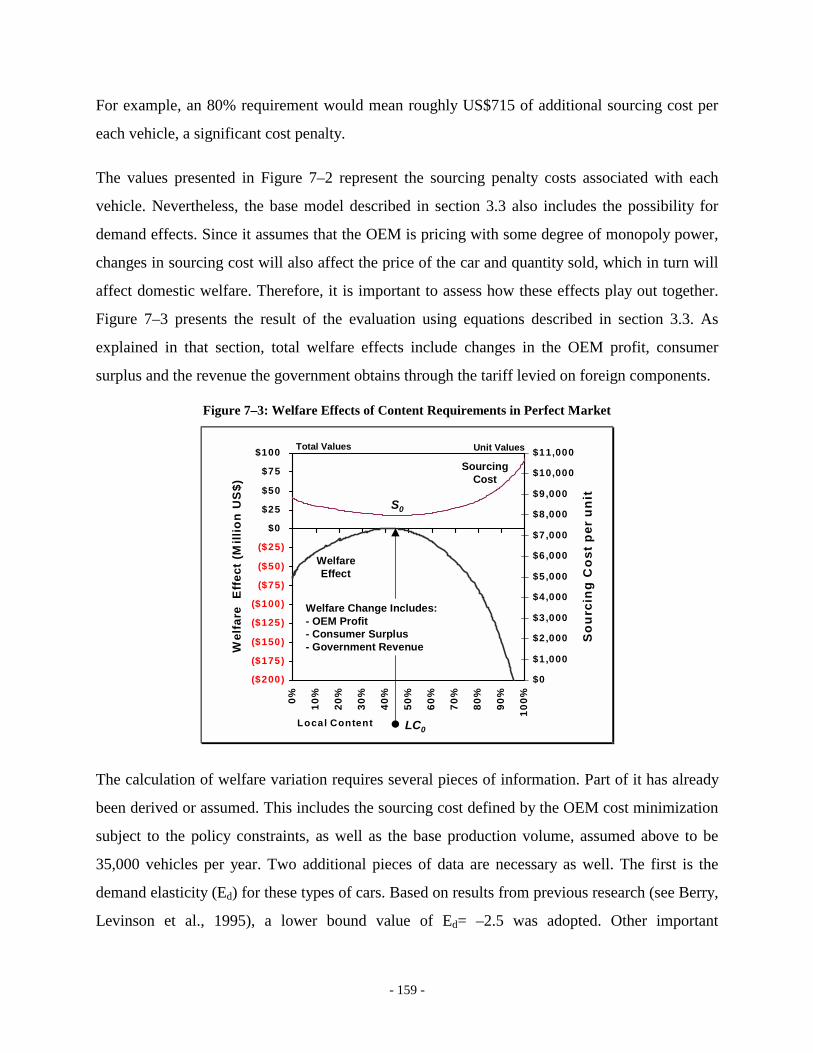
- 159 -

For example, an 80% requirement would mean roughly US$715 of additional sourcing cost per

each vehicle, a significant cost penalty.

The values presented in Figure 7–2 represent the sourcing penalty costs associated with each

vehicle. Nevertheless, the base model described in section 3.3 also includes the possibility for

demand effects. Since it assumes that the OEM is pricing with some degree of monopoly power,

changes in sourcing cost will also affect the price of the car and quantity sold, which in turn will

affect domestic welfare. Therefore, it is important to assess how these effects play out together.

Figure 7–3 presents the result of the evaluation using equations described in section 3.3. As

explained in that section, total welfare effects include changes in the OEM profit, consumer

surplus and the revenue the government obtains through the tariff levied on foreign components.

Figure 7–3: Welfare Effects of Content Requirements in Perfect Market

($200)

($175)

($150)

($125)

($100)

($75)

($50)

($25)

$0

$25

$50

$75

$100

0% 10%

20%

30%

40%

50%

60%

70%

80%

90%

100%

Local Content

Wel

fare

Eff

ect (

Mill

ion

US

$)

$0

$1,000

$2,000

$3,000

$4,000

$5,000

$6,000

$7,000

$8,000

$9,000

$10,000

$11,000

Sou

rcin

g C

ost p

er u

nit

Total Values

LC0

S0

Welfare Change Includes:- OEM Profit- Consumer Surplus- Government Revenue

WelfareEffect

SourcingCost

Unit Values

The calculation of welfare variation requires several pieces of information. Part of it has already

been derived or assumed. This includes the sourcing cost defined by the OEM cost minimization

subject to the policy constraints, as well as the base production volume, assumed above to be

35,000 vehicles per year. Two additional pieces of data are necessary as well. The first is the

demand elasticity (Ed) for these types of cars. Based on results from previous research (see Berry,

Levinson et al., 1995), a lower bound value of Ed= –2.5 was adopted. Other important

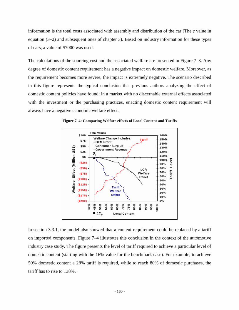
- 160 -

information is the total costs associated with assembly and distribution of the car (The c value in

equation (3–2) and subsequent ones of chapter 3). Based on industry information for these types

of cars, a value of $7000 was used.

The calculations of the sourcing cost and the associated welfare are presented in Figure 7–3. Any

degree of domestic content requirement has a negative impact on domestic welfare. Moreover, as

the requirement becomes more severe, the impact is extremely negative. The scenario described

in this figure represents the typical conclusion that previous authors analyzing the effect of

domestic content policies have found: in a market with no discernable external effects associated

with the investment or the purchasing practices, enacting domestic content requirement will

always have a negative economic welfare effect.

Figure 7–4: Comparing Welfare effects of Local Content and Tariffs

($200)

($175)

($150)

($125)

($100)

($75)

($50)

($25)

$0

$25

$50

$75

$100

40%

45%

50%

55%

60%

65%

70%

75%

80%

85%

90%

95%

100%

Local Content

Wel

fare

Eff

ect (

Mill

ion

US

$)

0%10%20%30%40%50%60%70%80%90%100%110%120%130%140%150%160%

Tari

ff L

evel

Total Values

LC0

S0

Welfare Change Includes:- OEM Profit- Consumer Surplus- Government Revenue

Tariff

LCRWelfareEffect

TariffWelfareEffect

In section 3.3.1, the model also showed that a content requirement could be replaced by a tariff

on imported components. Figure 7–4 illustrates this conclusion in the context of the automotive

industry case study. The figure presents the level of tariff required to achieve a particular level of

domestic content (starting with the 16% value for the benchmark case). For example, to achieve

50% domestic content a 28% tariff is required, while to reach 80% of domestic purchases, the

tariff has to rise to 138%.

- 161 -

The model also demonstrates the superiority of content requirements over tariffs as a policy

mechanism because it generates fewer distortions in the economy. The welfare impact of both the

content requirement and the tariff are presented on the left axis. The welfare effect for the tariff

policy is always substantially inferior to the one for the content requirement policy. For small

deviations away from the natural content level, the relative difference is particularly important.

For example, to increase the level of domestic content from 45% to 55%, content requirements

penalize the economy by 8.2 million dollars, 3% of the total base sourcing cost (unit cost times

quantity), while a tariff diminishes domestic welfare by 76 million dollars, 27% of the total base

sourcing cost.

7.2.2. The Social Opportunity Cost and the Welfare Effect of a Content Policy

The critical question the model addresses is the issue of social opportunity cost and externalities-

from-entry. The idea explained in section 3.4. is that there may be a gap between the social and

private costs for the resources used in the supplier activities. If this is the case, the content policy

may become valuable to the local economy.

Accurate estimates of the social opportunity costs of resources require a detailed investigation of

the economic conditions of the region where the investment is taking place. Since this thesis

discusses a generic evaluation of the local content policy rather than an analysis of a particular

project, a base set of average levels are considered and a sensitivity analysis to the values of these

parameters is done to make sure that the conclusions are not biased by the particular values that

were chosen.

For the application of the theoretical models to the auto industry case, the social opportunity cost

for the wages of the workers is considered to be half of the value paid by the firms, which results

in a 0.5 value for the parameter λ . This means that an alternative use for the labor only results in

half the result for the local economy. Following a similar logic for the cost of capital, each dollar

of capital used by the suppliers is assumed to have a social opportunity cost of 80 cents. As a

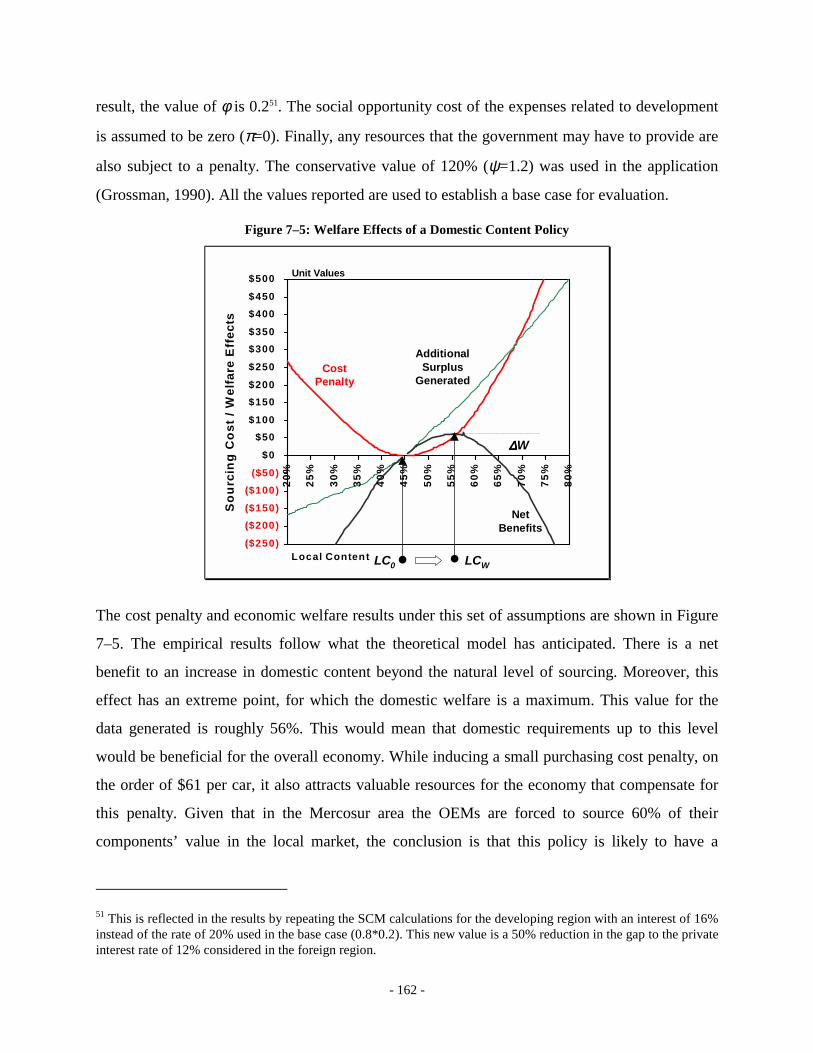
- 162 -

result, the value of φ is 0.251. The social opportunity cost of the expenses related to development

is assumed to be zero (π=0). Finally, any resources that the government may have to provide are

also subject to a penalty. The conservative value of 120% (ψ=1.2) was used in the application

(Grossman, 1990). All the values reported are used to establish a base case for evaluation.

Figure 7–5: Welfare Effects of a Domestic Content Policy

($250)($200)($150)($100)

($50)$0

$50$100$150$200$250$300$350$400$450$500

20%

25%

30%

35%

40%

45%

50%

55%

60%

65%

70%

75%

80%

Local Content

Sou

rcin

g C

ost /

Wel

fare

Eff

ects

Unit Values

LC0 LCW

∆∆∆∆W

Cost Penalty

AdditionalSurplus

Generated

Net Benefits

The cost penalty and economic welfare results under this set of assumptions are shown in Figure

7–5. The empirical results follow what the theoretical model has anticipated. There is a net

benefit to an increase in domestic content beyond the natural level of sourcing. Moreover, this

effect has an extreme point, for which the domestic welfare is a maximum. This value for the

data generated is roughly 56%. This would mean that domestic requirements up to this level

would be beneficial for the overall economy. While inducing a small purchasing cost penalty, on

the order of $61 per car, it also attracts valuable resources for the economy that compensate for

this penalty. Given that in the Mercosur area the OEMs are forced to source 60% of their

components’ value in the local market, the conclusion is that this policy is likely to have a

51 This is reflected in the results by repeating the SCM calculations for the developing region with an interest of 16% instead of the rate of 20% used in the base case (0.8*0.2). This new value is a 50% reduction in the gap to the private interest rate of 12% considered in the foreign region.

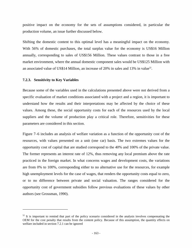
- 163 -

positive impact on the economy for the sets of assumptions considered, in particular the

production volume, an issue further discussed below.

Shifting the domestic content to this optimal level has a meaningful impact on the economy.

With 56% of domestic purchases, the total surplus value for the economy is US$16 Million

annually, corresponding to sales of US$156 Million. These values contrast to those in a free

market environment, where the annual domestic component sales would be US$125 Million with

an associated value of US$14 Million, an increase of 20% in sales and 13% in value52.

7.2.3. Sensitivity to Key Variables

Because some of the variables used in the calculations presented above were not derived from a

specific evaluation of market conditions associated with a project and a region, it is important to

understand how the results and their interpretations may be affected by the choice of these

values. Among these, the social opportunity costs for each of the resources used by the local

suppliers and the volume of production play a critical role. Therefore, sensitivities for these

parameters are considered in this section.

Figure 7–6 includes an analysis of welfare variation as a function of the opportunity cost of the

resources, with values presented on a unit (one car) basis. The two extremes values for the

opportunity cost of capital that are studied correspond to the 40% and 100% of the private value.

The former represents an interest rate of 12%, thus removing any local premium above the rate

practiced in the foreign market. In what concerns wages and development costs, the variations

are from 0% to 100%, corresponding either to no alternative use for the resources, for example

high unemployment levels for the case of wages, that renders the opportunity costs equal to zero,

or to no difference between private and social valuation. The ranges considered for the

opportunity cost of government subsidies follow previous evaluations of these values by other

authors (see Grossman, 1990).

52 It is important to remind that part of the policy scenario considered in the analysis involves compensating the OEM for the cost penalty that results from the content policy. Because of this assumption, the quantity effects on welfare included in section 7.2.1 can be ignored

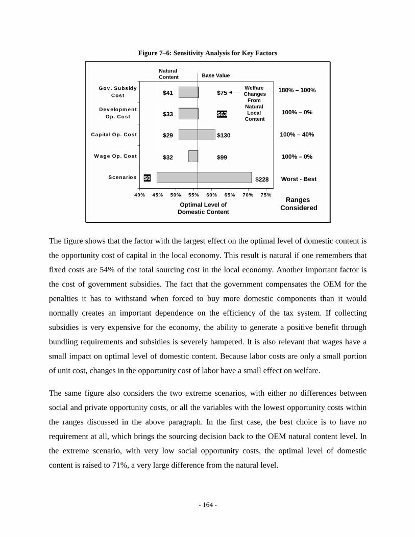
- 164 -

Figure 7–6: Sensitivity Analysis for Key Factors

40% 45% 50% 55% 60% 65% 70% 75%

Scenarios

W age Op. Cost

Capita l Op. Cost

Dev elopm entOp. Cost

Gov . SubsidyCost

180% – 100%

100% – 0%

100% – 40%

100% – 0%

Optimal Level of Domestic Content

$130

$228

$75

$99$32

$33 $63

$41

$0

$29

Base ValueNatural Content

Worst - Best

Welfare Changes

From Natural Local

Content

Ranges Considered

The figure shows that the factor with the largest effect on the optimal level of domestic content is

the opportunity cost of capital in the local economy. This result is natural if one remembers that

fixed costs are 54% of the total sourcing cost in the local economy. Another important factor is

the cost of government subsidies. The fact that the government compensates the OEM for the

penalties it has to withstand when forced to buy more domestic components than it would

normally creates an important dependence on the efficiency of the tax system. If collecting

subsidies is very expensive for the economy, the ability to generate a positive benefit through

bundling requirements and subsidies is severely hampered. It is also relevant that wages have a

small impact on optimal level of domestic content. Because labor costs are only a small portion

of unit cost, changes in the opportunity cost of labor have a small effect on welfare.

The same figure also considers the two extreme scenarios, with either no differences between

social and private opportunity costs, or all the variables with the lowest opportunity costs within

the ranges discussed in the above paragraph. In the first case, the best choice is to have no

requirement at all, which brings the sourcing decision back to the OEM natural content level. In

the extreme scenario, with very low social opportunity costs, the optimal level of domestic

content is raised to 71%, a very large difference from the natural level.

- 165 -

Scale is the other the key factor affecting manufacturing cost. Smaller production volumes affect

the component manufacturing cost and, as a consequence the natural level of domestic purchases

and the impact of any domestic content requirements. Figure 7–7 shows that very small

production volumes imply important decreases in the level of domestic content. At volumes on

the order of 5,000 cars per year, roughly 20% of the total purchases are done in the local

economy, while for 200,000 cars per year, the domestic content reaches almost 90%.

Figure 7–7: The implications of Volume for Domestic Content

$0

$1,000

$2,000

$3,000

$4,000

$5,000

$6,000

$7,000

$8,000

$9,000

$10,000

5,000 20000 35,000 75,000 100,000 200,0000%

10%

20%

30%

40%

50%

60%

70%

80%

90%

100%Sourcing Cost

Natural Local Content

($ 1 5 0 )

($ 1 2 5 )

($ 1 0 0 )

($ 7 5 )

($ 5 0 )

($ 2 5 )

$ 0

$ 2 5

$ 5 0

$ 7 5

$ 1 0 0

0 % 1 0 % 2 0 % 3 0 % 4 0 % 5 0 % 6 0 % 7 0 % 8 0 % 9 0 % 1 0 0%

L e v e l o f L o c a l C o n te n t R e q u ir e m e n t

Ne

t A

dd

itio

na

l Ec

on

om

ic B

en

e

5 ,0 0 0

2 0 ,0 0 0

3 5 ,0 0 0

7 5 ,0 0 0

1 0 0 ,0 0 0

2 0 0 ,0 0 0

Volumes

Unit Values

The production scale also affects the ability of the domestic content policy to have a positive

effect on the economy. For very small scales, the rise in the cost penalty curve is so steep that it

rapidly reaches the marginal benefit generated by forcing domestic purchases through regulation.

Therefore, for a production volume of 5,000 vehicles, the maximum benefit that the local

economy can reach through the content policy is negligible. On the contrary, as production

increases, there are greater potential welfare improvements from establishing such a policy.

These results show the determinant role of the relative curvature of the domestic and foreign cost

functions. If these are similar, the total cost curve will have a wide flat region around the

minimum, which means that there is a large leeway in substituting between domestic and foreign

components with minimum impact on the sourcing cost, but potentially important benefits for the

welfare of the domestic economy. On the contrary, a sharp difference in curvatures, usually due

to a technological gap between the regions will limit the ability to derive a positive result by

- 166 -

forcing domestic contents. This effect follows the logic presented in figure 5 of chapter 3. The

effects of production scale are a good example of how this relationship affects natural and

optimal domestic content levels.

These results indicate that within reasonable ranges of social opportunity cost for the relevant

variables, there is value to the enactment of modest levels of domestic content requirements. To

have a positive impact, these ought to be aimed at pushing the natural decisions of the OEMs

beyond what they would normally do. Nevertheless, there is a clear maximum benefit that can be

achieved and strict policies can have very harmful effects to an economy. Moreover, it is crucial

to recognize the role that scale plays. For very small scales, there is little potential welfare

improvements that can be generated through content requirements. Scale also indicates how

setting a blanket policy that is equal for all automakers and plants can have very different results.

While for some the impact can be positive, there are also others where it will be either negligible

or even negative.

7.2.4. Externalities and Learning Effects

The argument so far has relied on the notion of differences between social and private values for

the resources used in the industry. Parameters representing the potential gaps were considered to

in order to understand how their relative importance could justify the enactment of policies such

as domestic content requirements. Following the description of section 3.4.2, this section models

two situations that can drive this gap and result in sub-optimal decisions from private players: the

potential for learning by doing and then the possibility of learning by spillovers.

Before presenting the implementation of the model it is important to note that discussion is only

a first approximation to this complex problem. Give the approach used in chapter 5 to build up

the supplier’s cost structure, a detailed assessment of the learning effects should be grounded in

this model. This would require a careful modeling of how learning affects the use of resources

and the efficiency parameters of the manufacturer. This analysis is beyond the scope of the thesis.

Therefore, the choice to model learning as a direct effect on base cost is a first approximation to

the problem that bundles all the effects together. A detailed specification of the learning

mechanisms and their cost impact will be left for future work.

- 167 -

As explained in chapter 3, the existence of learning is associated with the cumulative output of

individual firms and the industry as a whole. Therefore, assessing its effect requires the

introduction of a time horizon for the project. In the context of the auto industry, the time horizon

considered will be five years. This period corresponds to the time over which a particular car

model retains similar characteristics and, as a result, the same supplier base (Veloso, Henry et al.,

2000, chapter 3). After this period, the OEM is likely to introduce significant design and

technical changes in the vehicle, or change the production to a completely different car. When

this happens, a new open bid for suppliers is usually conducted, which may result in significant

changes in the supplier base.

Following section 3.4.2., the effect of learning on the decisions is evaluated by minimizing

equation (3-31) with respect to i for particular values for the learning indexes γ and β and

comparing the results to the base situation with no learning (which corresponds to having

exponents equal to zero). The base discount rate used in the 5 year discounted sourcing cost

calculations will be the one considered in the evaluation of the cost of the domestic components.

In this case it will be 20%.

The level of domestic content over the 5-year period can be calculated by dividing the discounted

sum of the domestic purchases by the total discounted cost. While this value reflects the true

level of domestic content, it makes it hard to compare with the previous discussions that were

done on a year and unit basis and with a fixed cost. Therefore, learning effects are also discussed

by analyzing the first year level of domestic content. This value is calculated by dividing the cost

of domestic sourcing by the total cost in the first year of the five. Since, by construction, learning

and discounting only affect sourcing cost calculation starting in the second year, the first year

calculation of the local content value enables a good comparison of how much learning shifts the

firm decision to incorporate local components from the market base choice presented in Figure

7–5.

Initially, only learning by doing is assumed to be taking place. This means that the exponent β

will be zero. Figure 7–8 presents the results of the simulation. It considers values for the learning

parameter γ between 0 and 0.2, a range consistent with recent finding by other authors (Sinclair,

Klepper et al., 2000). Nevertheless, the horizontal axis is presented in terms of the learning slope

- 168 -

instead of the elasticity to facilitate perception (this calculated as 2-γ). The left axis has the total

five year discounted sourcing cost, while the right axis presents the five year average and the first

year equivalent levels of domestic content. As seen in the Figure, the maximum value of γ

corresponds to a cost reduction of 13% in total cost every time cumulative output doubles. This

extreme value implies that, in the fifth year, the cost of each domestic component is 76% of the

original cost. The drop in the cost of domestic components due to learning is reflected in the total

discounted sourcing cost. At the maximum learning rate, the total cost is 7% below its original

value.

Figure 7–8: Learning by Doing and Domestic Content

$20,000

$21,000

$22,000

$23,000

$24,000

$25,000

$26,000

$27,000

$28,000

$29,000

0% 2% 4% 6% 8% 10%

12%

14%

Slope of Learning Curve

Sou

rcin

g C

ost

44%

46%

48%

50%

52%

54%

56%

58%

60%

62%

64%

Dom

estic

Con

tent

Lev

el

Sum of Discounted Values over 5 years

5 yearAverage

Domestic Content

SourcingCost

7% Drop

1st yearDomestic Content

Because domestic cost is reduced over the project life, some components that are more expensive

than foreign equivalents in initial years will have a total discounted cost over the project time

below the imported counterparts total cost. These components, which would not be sourced

locally in the static analysis discussed in the previous sections, will now be part of the domestic

content. As a result, this is reflected in the share of sourcing that is done in the domestic market,

which increases with the learning rate53. As it can be seen in Figure 7–8, a learning curve slope

53 A careful analysis of the graph reveals that there are regions where the average domestic content curve is downward sloping. This happens because, unless a there is a change in the sourcing structure (change in the value if

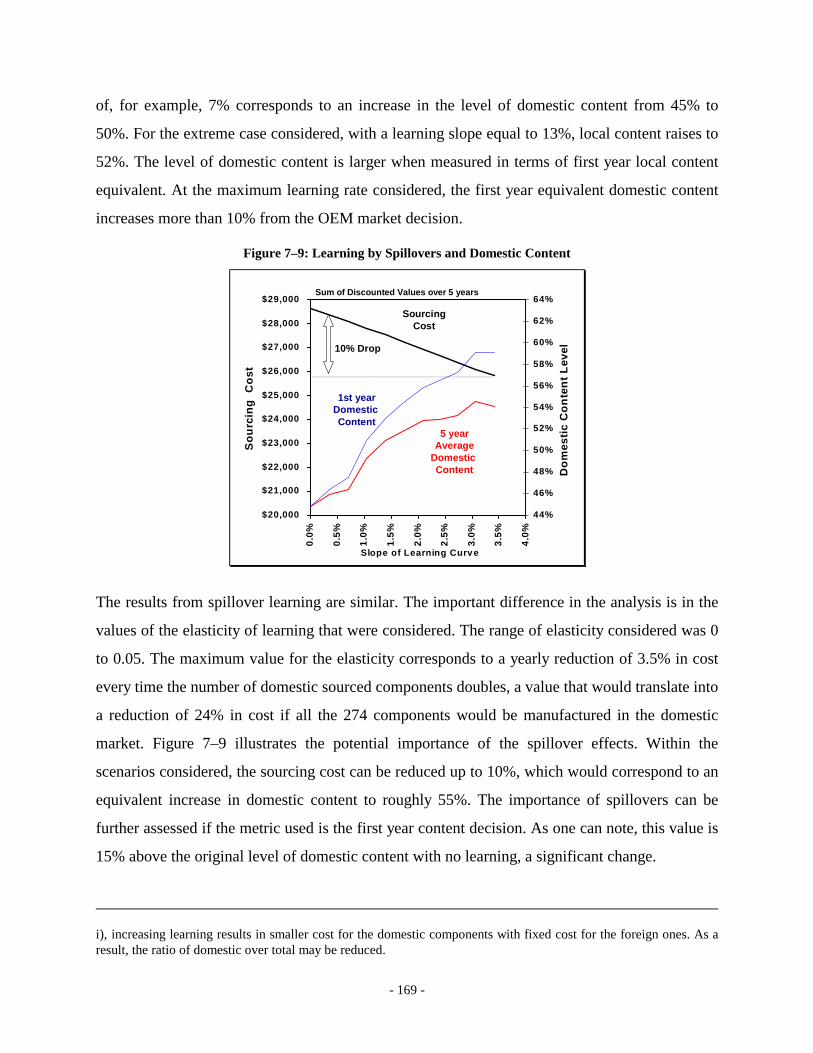
- 169 -

of, for example, 7% corresponds to an increase in the level of domestic content from 45% to

50%. For the extreme case considered, with a learning slope equal to 13%, local content raises to

52%. The level of domestic content is larger when measured in terms of first year local content

equivalent. At the maximum learning rate considered, the first year equivalent domestic content

increases more than 10% from the OEM market decision.

Figure 7–9: Learning by Spillovers and Domestic Content

$20,000

$21,000

$22,000

$23,000

$24,000

$25,000

$26,000

$27,000

$28,000

$29,0000.

0%

0.5%

1.0%

1.5%

2.0%

2.5%

3.0%

3.5%

4.0%

Slope of Learning Curve

Sou

rcin

g C

ost

44%

46%

48%

50%

52%

54%

56%

58%

60%

62%

64%

Dom

estic

Con

tent

Lev

el

Sum of Discounted Values over 5 years

5 yearAverage

Domestic Content

SourcingCost

10% Drop

1st yearDomestic Content

The results from spillover learning are similar. The important difference in the analysis is in the

values of the elasticity of learning that were considered. The range of elasticity considered was 0

to 0.05. The maximum value for the elasticity corresponds to a yearly reduction of 3.5% in cost

every time the number of domestic sourced components doubles, a value that would translate into

a reduction of 24% in cost if all the 274 components would be manufactured in the domestic

market. Figure 7–9 illustrates the potential importance of the spillover effects. Within the

scenarios considered, the sourcing cost can be reduced up to 10%, which would correspond to an

equivalent increase in domestic content to roughly 55%. The importance of spillovers can be

further assessed if the metric used is the first year content decision. As one can note, this value is

15% above the original level of domestic content with no learning, a significant change.

i), increasing learning results in smaller cost for the domestic components with fixed cost for the foreign ones. As a result, the ratio of domestic over total may be reduced.

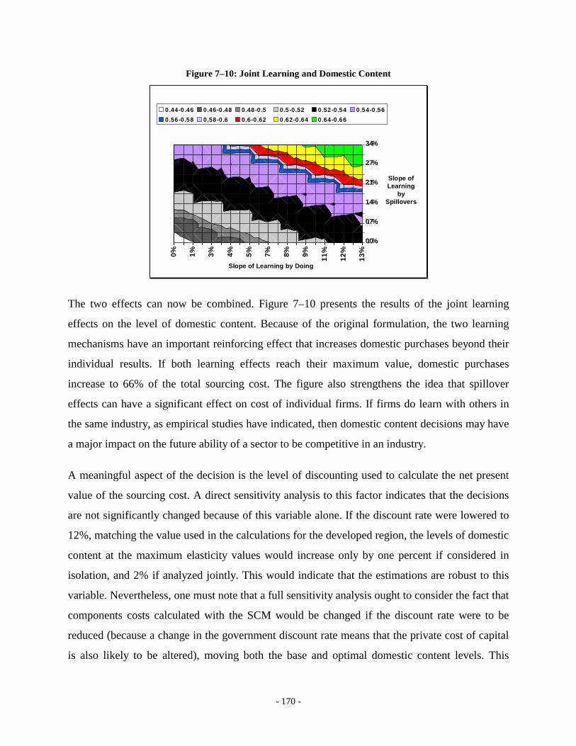
- 170 -

Figure 7–10: Joint Learning and Domestic Content

0% 1% 3% 4% 5% 7% 8% 9% 11%

12%

13%

0.0%

0.7%

1.4%

2.1%

2.7%

3.4%

0.44-0.46 0.46-0.48 0.48-0.5 0.5-0.52 0.52-0.54 0.54-0.560.56-0.58 0.58-0.6 0.6-0.62 0.62-0.64 0.64-0.66

Slope of Learning by Doing

Slope of Learning

by Spillovers

The two effects can now be combined. Figure 7–10 presents the results of the joint learning

effects on the level of domestic content. Because of the original formulation, the two learning

mechanisms have an important reinforcing effect that increases domestic purchases beyond their

individual results. If both learning effects reach their maximum value, domestic purchases

increase to 66% of the total sourcing cost. The figure also strengthens the idea that spillover

effects can have a significant effect on cost of individual firms. If firms do learn with others in

the same industry, as empirical studies have indicated, then domestic content decisions may have

a major impact on the future ability of a sector to be competitive in an industry.

A meaningful aspect of the decision is the level of discounting used to calculate the net present

value of the sourcing cost. A direct sensitivity analysis to this factor indicates that the decisions

are not significantly changed because of this variable alone. If the discount rate were lowered to

12%, matching the value used in the calculations for the developed region, the levels of domestic

content at the maximum elasticity values would increase only by one percent if considered in

isolation, and 2% if analyzed jointly. This would indicate that the estimations are robust to this

variable. Nevertheless, one must note that a full sensitivity analysis ought to consider the fact that

components costs calculated with the SCM would be changed if the discount rate were to be

reduced (because a change in the government discount rate means that the private cost of capital

is also likely to be altered), moving both the base and optimal domestic content levels. This

- 171 -

analysis requires a more detailed framework that relates the micro variables used in the SCM

with the learning dynamics, something that will not be addressed in the thesis.

As noted in the discussion of section 3.4.2., if the presence of learning effects is anticipated or

known by OEM, it would naturally lead to higher levels of domestic purchases. The firm would

incorporate the new price regime in the sourcing decision, finding the optimal solution to the

problem from a private as well as social perspective. The natural level of domestic content would

be the one presented in the figures above, conditional on the relative importance of learning.

The problem arises if learning is not recognized or accepted by the OEM, or impossible to

measure ex-ante. If this were the case, the firm would make the base decision with no learning.

Therefore, it becomes clear from the figures presented above that both the investing firm and

domestic economy would benefit if government required a level of domestic content that

accounted for the learning potential. This situation embodies the well known infant-industry

protection argument, whereby because of myopic economic agents or coordination problems, the

government establishes restrictive policies to allow learning from domestic producers, but with

the understanding that the total welfare of the country will be improved (Dasgupta and Stiglitz,

1988; Grossman, 1990).

When enacting domestic requirements, the government should also be aware of their impact on

the incentives of the economic agents. If suppliers see the market as guaranteed, they may slack

and not learn as much as they would if pressed by a contract. On the other hand, they may

effectively go down the learning curve, but do not reflect that in the cost of the components to

extract rents from the contract. A potential solution to this problem is to enact contracts that

require price reductions over time, meeting the expected effect of the learning curve. In fact, the

establishment of contracts between OEMs and suppliers that have price reductions clauses are

common practice in the industry, even in contexts without any type of domestic requirements

(Clark and Veloso, 2000).

An important aspect to note is that within the reasonable levels of learning considered in the

analysis, the optimal domestic sourcing decisions are similar to those justified through gaps in

the valuations of the critical resources exposed in section 7.2.2. It we assume that learning effects

- 172 -

are embedded in the use of capital and human resources in the suppliers, the two approaches

converge. The idea is that each worker and each unit of capital embodies, not only its direct

productive use that results in the component that is delivered to the OEM, but also a future

learning potential that is not valued and paid by the market. This learning potential generates the

gap between private and social opportunity costs. The underlying assumption is that the

government must be able to see or value this learning better than the economic agents.

Otherwise, it would be incorporated in the decisions of both the OEM and local suppliers. To the

extent that learning is external and difficult to value ex-ante, this situation becomes more likely.

Another reason that could lead the OEM to underestimate the importance of learning could be

management risk aversion. If learning happens only with a certain probability, then a risk averse

purchasing manager might prefer a foreign supplier with a cost for sure to a domestic supplier

with a lower expected cost but a non zero chance of a higher cost than the foreign alternative.

This aspect will be detailed in the next section.

7.2.5. Risk Averse Decisions

Understanding the effect of risk aversion from the OEM managers is very close to the situation

described above where potential learning effects are not recognized. As described in section 3.5,

the focus is on a situation where the prices of domestic components have a normal distribution

around a mean value, rather than a certain value, together with the fact that the purchasing

manager is risk averse. Under certain assumptions, this situation can be described by replacing

the original price by 2. 2i

rPP Di

Di εσ+→ , where r is the degree of risk aversion and σi

2 is the

variance of the price of component i.

The importance of risk aversion depends on the potential variances associated with prices and

with the degree of risk aversion. The variance is taken to be a share of the price of the

component, varying between zero and half the expected price54. The coefficient of risk aversion

54 A more general model could be considered, but that would mean that the component index generated through increasing cost ratio would no longer be valid. The solution could be achieved through a mixed integer programming analysis, that would yield similar results, although of less intuitive analysis.

- 173 -

will be assumed to go from zero to 1.25, to be able to evaluate a wide spectrum of risk aversion.

The results of the estimates are presented in Figure 7–11.

As it can be seen from the figure, the impact of risk aversion on the degree of domestic content

can be quite significant. Risk averse purchasing managers that face local component costs with

variances below 35% of the expected cost will substantially reduce their level of domestic

purchasing. These variances are rather small. For the average component that is bought by the

OEM, which costs on the order of $35, this variance represents a standard deviation in cost on

the order of $3.5, 10% of the price. As one would expect, as the degree of risk aversion is

reduced, the impact on the level of domestic cost is much reduced.

Figure 7–11: The Impact of Risk Aversion in Domestic Sourcing

15%

20%

25%

30%

35%

40%

45%

50%

0% 5% 10%

15%

20%

25%

30%

35%

40%

45%

50%

Price Variance (share of component price)

Dom

estic

Con

tent

1 .2510.750.50.25

Coefficient Of

Risk Aversion

The reason small uncertainties on cost have an important impact on the level of domestic content

is very similar to the reason that differences between private and social opportunity costs affect

the level of domestic content, only with the reverse interpretation. As described in section 7.2.1,

there are a large number of components whose cost difference between domestic and foreign

sourcing is very small. Therefore, forcing some of these to be bought in the local economy

beyond what would be natural generates a limited sourcing cost penalty, which may be

overcompensated by the additional benefits that result from the differences in opportunity cost.

- 174 -

The risk-averse manager has precisely the opposite logic. Because there is a range of components

with small differences in expected cost, even a small uncertainty will make him choose the

foreign supplier with a price for sure, rather than a domestic one with uncertainty on cost. The

idea is that, because the potential cost penalty of the imports is small, he prefers not to take any

chances. The remedy discussed in section 3.5 may be the establishment of a preemptive domestic

requirement that counters the aversion of the purchasing manager. If it enacts a regulation that is

equal to the base level of domestic content, it forces the manager to choose the solution that an

equivalent risk neutral manager would choose, with obvious benefits for the local economy.

7.3. Incentive Contracts, Asymmetric Information and Content Decisions

The previous section implemented the overall framework and the models discussed in chapter 3.

It discussed the implications of domestic content policies for a range of market conditions,

analyzing the circumstances under which the domestic market may benefit from this policy, as

well as those where it is likely to hurt the economy. This section follows the approach and

models presented in chapter 4. This chapter addressed contractual conditions and the

mechanisms that local governments may use to maximize the benefit of the policy in the

domestic market. In particular, it showed that, instead of demanding content levels, it was

possible to establish incentive schemes that would lead the OEM to make the sourcing decisions

according to the desires of the local government. This section presents the application of these

models to the context of the automotive case study that has been the object of this chapter.

7.3.1. The Optimal Incentive Contract

Section 4.3.1 described the general case whereby the government receives increasing benefits

from higher levels of domestic purchases, but the firm faces additional costs resulting from this

increase in content. The equilibrium solution matches the findings of chapter 3. The general

result is that components will be sourced in the domestic market until the marginal benefit to the

government matches the marginal cost resulting from the subsidies awarded to compensate the

OEM for the cost penalties it has to endure. The section also showed that, if both the government

and the firm were aware of the cost structure of the components, it was possible to establish an

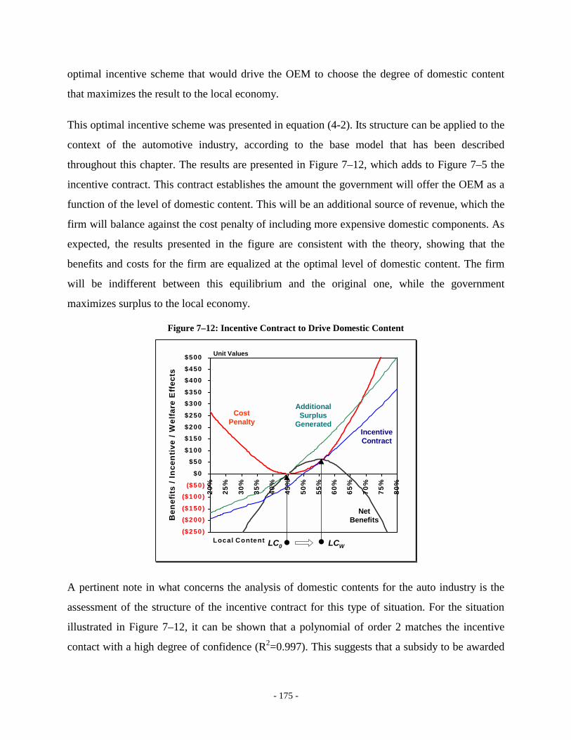
- 175 -

optimal incentive scheme that would drive the OEM to choose the degree of domestic content

that maximizes the result to the local economy.

This optimal incentive scheme was presented in equation (4-2). Its structure can be applied to the

context of the automotive industry, according to the base model that has been described

throughout this chapter. The results are presented in Figure 7–12, which adds to Figure 7–5 the

incentive contract. This contract establishes the amount the government will offer the OEM as a

function of the level of domestic content. This will be an additional source of revenue, which the

firm will balance against the cost penalty of including more expensive domestic components. As

expected, the results presented in the figure are consistent with the theory, showing that the

benefits and costs for the firm are equalized at the optimal level of domestic content. The firm

will be indifferent between this equilibrium and the original one, while the government

maximizes surplus to the local economy.

Figure 7–12: Incentive Contract to Drive Domestic Content

($250)($200)($150)($100)

($50)$0

$50$100$150$200$250$300$350$400$450$500

20%

25%

30%

35%

40%

45%

50%

55%

60%

65%

70%

75%

80%

Local Content

Ben

efits

/ In

cent

ive

/ Wel

fare

Eff

ects

Unit Values

LC0 LCW

AdditionalSurplus

Generated

Net Benefits

IncentiveContract

CostPenalty

A pertinent note in what concerns the analysis of domestic contents for the auto industry is the

assessment of the structure of the incentive contract for this type of situation. For the situation

illustrated in Figure 7–12, it can be shown that a polynomial of order 2 matches the incentive

contact with a high degree of confidence (R2=0.997). This suggests that a subsidy to be awarded

- 176 -

to the investing OEM ought have an increase that is more aggressive than a linear dependence on

the commitment of the firm to buy domestic components beyond its market level ( Subsidy = -

52.3 + 1751.3(LC-45%)2 + 862.28(LC-45%) ).

The shape of the incentive contract is determined by the benefit curve associated to the inclusion

of domestic components. Sensitivity analysis to the various scenarios exposed in Figure 7–6 and

a range of production volume indicates that, in general, an incentive contract for the auto industry

with the aim of inducing higher levels of domestic content ought to be more aggressive than a

linear one, but less than a full quadratic relationship.

7.3.2. Degree of Uncertainty, Government Menus and Firm Decisions

The results discussed in 4.3.1 and the application presented in the previous section relied on the

assumption that the firm and the government had the same information regarding the cost

structures of the components to be purchased. Nevertheless, there may be situations where this

assumption is not true. In fact, it is reasonable to suppose that the OEM has more information

than the government regarding the true costs of the components and that it tries to use it for its

own advantage. Section 4.3.2 developed a simple model to study these effects, considering

differences both in the cost penalty and in the benefits generated by increasing domestic

purchases from the investing firm. The objective was to understand how this situation would

affect the ability of the Government to enact efficient content policies, in particular its ability to

establish incentive contracts. This section applies the asymmetric information model to the auto

industry case study.

The application considers that the true cost of the domestic components is private information of

the OEM. Domestic components will have either a base cost similar to the one presented in the

section above (corresponding to the low cost β firm), or face a cost that includes an additional

penalty (corresponding to high cost β ). The penalty is treated as a percentage increase over the

base cost for every component that is bought in the domestic market. The OEM will be aware of

which of the situations is true, but not the government, which will nevertheless know the

probability that the cost of the domestic components cost is either the base cost or the high cost.

- 177 -

The benefit side is simplified, allowing each component to generate an identical surplus effect,

regardless of its true cost55

The results of the theoretical model, detailed in Chapter 4, indicated that the incentive contract

involves offering the investing OEM a menu that includes both a level of required domestic

content and an associated subsidy targeted to the base cost ),( et→β , as well as one aimed

towards the high cost scenario ),( et→β . The objective is to structure these offers to make sure

that the OEM selects the option that fits its true cost structure, therefore revealing its type and

maximizing the benefits to the local economy. The calculations show that the best incentive

scheme that can be derived leads to an optimal choice of domestic content if the firm has the

lower (base) cost, equivalent to the one that would be chosen in the case of full information, but a

potential sub-optimal level of domestic content if the high domestic cost situation is verified. It

also explains that the firm with the base cost will be able to extract subsidies from the

government that go beyond what it would receive with full information.

The reason for inefficient contracting is the ability of the low cost firm to mimic the behavior of

the firm with high sourcing costs. To make sure that the OEM facing base costs chooses the

optimal levels of domestic content and does not mimic the high cost behavior, the government

uses two complementary mechanisms that drive the inefficiency of the contract: it may be less

ambitious in the incentive contract towards the high cost and it may also award a subsidy

targeting the base cost scenario that is greater than the value it would award with full

information.

The auto application results for this second best contracting arrangement involve menus targeted

both at the base cost and the high cost scenarios. For the menu targeted at the base case cost, a

domestic content of 56% is always demanded (equal to the full information optimal content

level) and the corresponding subsidy depends on the probability that the government is facing a

55 A general discussion would consider the added costs to be generated by different underlying sourcing conditions (e.g. line efficiency) that would also affect the benefits generated to the domestic economy. Such an analysis was performed with similar results to those that are presented here. Nevertheless, because the interpretation of the full variation is less obvious, this simpler analysis is considered

- 178 -

higher domestic sourcing cost scenario and the particular cost penalty associated to it. The values

for this subsidy transfer (represented as ),( ξρt ) as a function of the probability of facing this

higher domestic cost (ξ) and for several cost penalty scenarios (ρ) are shown on the right hand

side of Figure 7–13. The left hand side shows the level of domestic content requirement targeted

for the high cost scenario as a function of the same variables ( ),( ξρe ). The subsidy transfer for

the high cost scenario, not shown in the graphs, is calculated as the value that exactly matches the

cost penalty associated to reaching the required content level ( )(et ). The set of menus offered by

the government can be represented as ( ) ( ){ })(),,(;),(%,56 etet ξρξρ .

Figure 7–13: Menu of Contracts Offered as a Function of Uncertainty

30%

35%

40%

45%

50%

55%

60%

0% 10%

20%

30%

40%

50%

60%

70%

80%

90%

100%

Probability of Base Cost

Loca

l Con

tent

Hig

h C

ost

Unit Value

$50

$60

$70

$80

$90

$100

0% 10%

20%

30%

40%

50%

60%

70%

80%

90%

100%

Probability of Base Cost

Tran

sfer

to L

ow C

ost F

irm

0%4%8%12%

Unit Value

HighCost

Penalty

On the left hand side of Figure 7–13, it is possible to note that, if the government knows for sure

that the OEM faces high costs (probability equal to zero), it will offer an optimal (first best)

contract, similar to the one described in the beginning of the section, but adjusted to the higher

cost conditions. Nevertheless, as the probability of facing base costs increases, the government

will demand less content and award correspondingly lower subsidies for the high cost situation,

eventually reaching the natural level of domestic content for the particular sourcing conditions

(the domestic content when probability is one). When the domestic content reaches the natural

level, the government stops considering it to be worthwhile to induce extra content from the high

cost situation and will offer no subsidy at all. This is the extreme case of presenting the OEM

- 179 -

with the choice of either no requirement and no subsidy, or a particular requirement and

associated subsidy.

The ability of the lower cost OEM to extract extra rents from the government is clearly seen on

the right hand side of the figure. To assure that the OEM does not mimic the higher cost

situation, the government awards it with a subsidy that is greater than the value given out in the

situation of full information (domestic content in the base cost scenario is always at the optimal

level). As the probability of encountering a base cost situation increases, the need to award the

extra subsidy is reduced, eventually reaching the base value of $61 dollars paid in the case of full

information. Comparing the two graphs of Figure 7–13, it is also possible to see that a reduction

in the probability of the base cost leads the government, initially to reduce the domestic content

requirements in the part of the menu targeted for the higher cost situation, and only afterwards to

start awarding extra subsidies to the base cost scenario.

An increasing gap between the base and the high cost scenarios has a different impact on in the

two mechanisms discussed. The need to reduce content requirements for the high cost scenario is

aggravated, since the ability to demand the optimal level of domestic content is reduced with the

increasing cost penalty. The need to consider extra subsidies to the lower cost firm is less

prevalent in the full range of probabilities as the cost penalty increases, but the values of these

extra rents tend to be higher for greater cost penalties, up to a point. When the optimal level of

domestic content for the high cost OEM reaches values close to the natural level of the base cost

situation, the problems become separated and the need to award large rents is reduced. This is the

reason why the transfer value with an 8% cost penalty is higher than the value for both the 4%

and the 12% penalty levels. The separation is driven by the assumption that the OEM facing a

base cost does not have an incentive to go below the natural level of domestic content. As a

result, if the optimal domestic content for the high cost is below the natural content level for the

base cost, the government offers a menu with two potential contracts that do not interact, the

separation will be complete and the contract becomes efficient again.

Because asymmetric information limits the possibility of the government to establish efficient

incentive contracts, its ability to maximize domestic welfare is reduced. This result is presented

in Figure 7–14. To understand this reduction note that net welfare gains do not vary linearly with

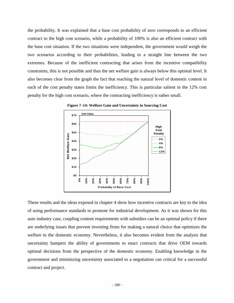
- 180 -

the probability. It was explained that a base cost probability of zero corresponds to an efficient

contract to the high cost scenario, while a probability of 100% is also an efficient contract with

the base cost situation. If the two situations were independent, the government would weigh the

two scenarios according to their probabilities, leading to a straight line between the two

extremes. Because of the inefficient contracting that arises from the incentive compatibility

constraints, this is not possible and thus the net welfare gain is always below this optimal level. It

also becomes clear from the graph the fact that reaching the natural level of domestic content in

each of the cost penalty states limits the inefficiency. This is particular salient in the 12% cost

penalty for the high cost scenario, where the contracting inefficiency is rather small.

Figure 7–14: Welfare Gain and Uncertainty in Sourcing Cost

$0

$10

$20

$30

$40

$50

$60

$70

0% 10%

20%

30%

40%

50%

60%

70%

80%

90%

100%

Probability of Base Cost

Net

Wel

fare

Gai

n

0%4%8%12%

Unit Value

HighCost

Penalty

These results and the ideas exposed in chapter 4 show how incentive contracts are key to the idea

of using performance standards to promote for industrial development. As it was shown for this

auto industry case, coupling content requirements with subsidies can be an optimal policy if there

are underlying issues that prevent investing firms for making a natural choice that optimizes the

welfare to the domestic economy. Nevertheless, it also becomes evident from the analysis that

uncertainty hampers the ability of governments to enact contracts that drive OEM towards

optimal decisions from the perspective of the domestic economy. Enabling knowledge in the

government and minimizing uncertainty associated to a negotiation can critical for a successful

contract and project.

- 181 -

7.4. Summary

This chapter analyzes the specific context of domestic content requirements, integrating the

theoretical models presented in chapters 3 and 4 with the system cost model proposed in chapter

5 and the specific context of the auto industry supply chain presented in chapter 6.

The base scenario considers a market with no discernable external effects associated with the

investment or the purchasing practices. The results confirm the typical conclusion that previous

authors analyzing the effect of domestic content policies, whereby enacting domestic content

requirement will always have a negative economic welfare effect. Similarly, it is also shown that

the welfare effect of a tariff policy is always substantially inferior to the one resulting from a

content requirement. For small deviations away from the natural content level, the magnitude of

the relative difference is particularly important as tariffs may reduce welfare as much as nine

times more than domestic content.

In the presence of external effects, the results confirm that there is a net benefit to an increase in

domestic content beyond the natural level of sourcing. For the base case considered in the

analysis, shifting the domestic content to this optimal level has a meaningful impact on the

economy, with annual domestic sales of components increasing by 20% and the net external

value growing by 13%. Nevertheless, the optimal level of domestic content and the related

market effects depend on a number of variables, in particular the production volume of the

vehicle and the opportunity cost of capital. Therefore, domestic content policies should be

considered case-by-case. For very small scales, in particular, there seems to be little potential

welfare improvements that can be generated through content requirements.

The model evaluation is then used to consider explicit learning mechanisms associated with

cumulative output of the industry and the firm. As expected, these effects justify an increase in

the level of domestic content An important aspect to note is that, within the reasonable levels of

learning considered in the analysis, the optimal domestic sourcing decisions are similar to those

justified through gaps in the valuations of the critical resources. If one considers that learning

effects are embedded in the use of capital and human resources in the suppliers, then the two

approaches converge and the comparable empirical results work as a confirmation of this idea.

- 182 -

The contracting analysis shows that, for the particular situation considered, a polynomial of order

2 matches the incentive contact with a high degree of confidence. In the presence of asymmetric

information the incentive contract involves offering the investing OEM a menu that includes

both a level of required domestic content and an associated subsidy targeted to the base cost as

well as one aimed at the high cost scenario. The results show the expected contract inefficiency

that results from the differences in information between the government and the firms, but only

up to a point. Large cost gaps create a natural separation between potential players that enable the

government to offer two contracts without the problem of having the low cost firm mimicking

the high cost one.

Finally, the analysis associated with risk averse purchasing managers shows how this is pressing

problem, as it may lead to substantial reductions in the level of domestic purchasing, even with

modest uncertainty on domestic component costs.

- 183 -

Chapter 8. Conclusions and Future Work

8.1. Conclusions

This thesis addresses the question of performance standards in developing nations, focusing on

the role of local content requirements. Initial chapters proposed a theoretical framework to

understand the impact of these policies on the decisions of the firms and the welfare of the

domestic economy, while the later chapters offer a methodology to apply the analysis for the

context of the automotive industry.

The first important conclusion deriving from the theoretical analysis presented in chapter 3 is that

the policy of content requirements is superior to the use of tariffs and subsidies as a means to

increase the share of domestic purchases from the OEM. The key intuition as to why this may be

the case is the fact that the government is setting a standard, but relying on the OEM to make the

decisions on how to comply, the government benefits from the firm’s ability to minimize

potential negative impacts on its cost and, as a result, on the overall economy.

The second and central conclusion of the thesis relates to the existence of gaps between private

and social opportunity costs of the resources employed in the OEM and its suppliers. In a

developing country, a new foreign OEM investment generates a unique occasion for a set of local

firms to enter into the manufacturing of complex products. Because of spillovers and learning

effects, this possibility tends to propel the overall capability of the industry to levels that would

not be attainable by alternative means. In some circumstances, these industry external effects

may not be accounted in the valuations of private economic agents. If these effects depend on the

breadth of the supplier structure, there will be an externality-from-entry associated with domestic

suppliers that drives a gap between social and private valuation. This gap generates the

opportunity for the enactment of domestic content requirements. The analysis shows that local

- 184 -

content requirements can improve welfare as long as the opportunity cost gap of the components

sourced beyond the OEM market decision is above the cost penalty associated with them.

Chapter 4 discusses implementation. Subsidies and requirements coupled through reciprocity

principles act as incentive mechanisms that align the OEM decision with the optimal for the

domestic economy. Nevertheless, the analysis also shows that uncertainty concerning the effects

of content requirements on the cost structures of the firms reduces the ability of the government

to have efficient incentive contracts and thus to improve domestic welfare.

A case study for the automotive industry, where content restriction policies are extremely active,

is used to demonstrate the applicability of the model. This entailed the development of a new

methodology, called Systems Cost Modeling (SCM), which proposes simple metrics and rules to

build bottom-up cost structures where estimates for large number of components have to be

considered. Detailed empirical data from a particular car is then used to build a sourcing cost

structure. These costs are integrated with the content model to show that, for existing market and

policy conditions there is value to the enactment of modest levels of domestic content

requirement in the auto industry. It also shows that the impact of the policy is very sensitive to

project characteristics and that this should be factored in the policy decisions of the nations.

There are also a number of insights that the model and application provide:

• The social opportunity cost requirement. Domestic content requirements are relevant for

economies when differences between social and private opportunity costs exist. In an

economy where social and private cost of the resources used in manufacturing components

that result from the requirement policy are close, the requirement policy is bound to have a

negative effect. This could be because the knowledge is already present or because there are

alternative uses for the resources that are equally beneficial for the society. This is the case in

advanced economies, where the same resources devoted to research and development are

likely to generate greater benefits to the society.

• Value at the margin. Domestic content requirements are likely to be effective in regions

where the overall technology gap of the components that are forced into local production is

- 185 -

small. In this situation, the cost penalty is likely to be small and the region is able to realize

the most from potential external-benefits from entry.

• Unique policies are not feasible. As illustrated, the optimal level of domestic content depends

on a number of variables, in particular the production volume of the vehicle. Therefore, it is

insufficient to establish only one measure of domestic content, but rather it should part of a

case-by-case negotiation.

• Coupling requirements and subsidies is optimal. Coupling content requirements with

subsidies can be an optimal policy to drive investing firms to make a choice that optimizes

the welfare of the domestic economy without hurting their competitive ability. Nevertheless,

uncertainty hampers the ability of governments to enact these contracts.

• Greedy government. Domestic requirements have a clear upper bound. Therefore,

governments that are too greedy and demand too high a level of content are likely to severely

hurt the economy. In adverse situations, often associated with small production volumes, it

may be virtually impossible to have a positive effect from the regulation.

• Cooperative approaches. Governments and firms are likely to mutually gain by cooperating

up-front in the decisions regarding local purchasing and subsidies. A careful balance between

the two aspects is likely to propel the economy into a higher level of welfare, while leaving

the investing firm indifferent.

• The importance of learning. As shown in the analysis, the presence of learning effects that are

not internalized in the decisions of the firms can justify the enactment of content

requirements. Moreover, they will benefit both the investing firm and the local economy.

• Risk averseness. Domestic content requirements can also be used to dampen potential risk

averse behavior from the purchasing manager at the local plant.

These conclusions provide a good explanation regarding why it is possible to find situations

where domestic content requirement have had a positive effect on the economy and others where

the policy is disastrous. A government that forces high levels of domestic content in a context

- 186 -

where cost penalties are high will never be able to recoup the costs to the economy through

external effects. It also helps to explain why, in situations where the cost penalty is small (and

often paid by subsidies) and local jobs are being generated, managers in the investing OEM may

feel indifferent or even have a positive attitude towards local content requirements. A final aspect

that the analysis presented in this thesis exposes the need for additional empirical research

associated with the conditions under which linkages generate learning in the local firms.

8.2. Future Work

As expected, the research work raises a number of additional questions that are not directly

addressed in the work presented here. Some of these that are of particular significance in terms of

future work are discussed below.

The analysis of the thesis has shown that the results of the models are sensitive to the ability of

local suppliers to improve their manufacturing cost through learning. Therefore, this is an area

where it is important to develop further research. While learning has been considered an

exogenous mechanism in this dissertation, it is important to change this aspect and incorporate

endogenous supplier learning.

The intuitive idea is that if local suppliers are expected to learn as they work with foreign

multinationals, government could be more aggressive in terms of local content requirements.

Nevertheless, because these same local firms may feel that they are shielded by government

regulation, they may have fewer incentives to invest in learning. Understanding the dynamics of

this relationship is the objective of this section of the proposed research.

Another area where further work is appropriate is in the decision of the OEM to invest. The

research presented in the dissertation assumes the decision to invest in the particular region under

analysis to have already taken place. Nevertheless, competition for foreign investments has

become increasingly important. Therefore, it is important to understand how competition for

foreign investment may affect the results of the models presented in the dissertation. The avenue

to pursue is to couple the models discussed in the thesis with a model of government competition

for multinational investment.

- 187 -

One of the aspects of the thesis where significant future development can be made is in the

System Cost Model described in chapter 5. The critical issue is refining the estimation process

used for each of the technologies. This will entail gathering component and processing

conditions data for each process to enable more accurate estimates of the functional relationships

between component characteristics and fixed costs, labor utilization and cycle time. The first step

is refining the factor relations that establish the relative importance of complexity and weight. A

second step is to have enough information to enable direct regression estimates.

A different level of development is related to alternative applications of the systems cost model

in the study of global supply chain dynamics, in the auto industry or elsewhere. The ability to

have estimates for the complete supply chain cost structure of a product, as well as the capacity

to evaluate cost sensitivity to key parameters, can be of relevance to examine issues ranging from

distribution strategies to global capacity management or e-commerce cost savings. Any of them

provide an avenue of research that can be pursued.

- 188 -

Chapter 9. Appendix

9.1. Appendix with Details of the Demonstrations of Chapter 4

9.1.1. Calculations for Asymmetric Information

First, the implications of the four constraints for the behavior of both the government and the

firms are examined. First lets consider the ICCs. Adding them up one gets:

⇔≥−−+ 0),(),(),(),( ββββ eSeSeSeS

0),(0),(),()(

)(

'''' ≤⇔≥−⇔ ∫ ∫∫=

=

ββββββ

β

β

ββ

β

βββ dedeSdeSeS

ee

eee

For this to be verified, the profit function of the firms should verify the single crossing property

(SC), which can be translated as:

0),(0),(0 ''2

>⇔>∂∂

∂⇔>

∂Π∂

∂Π∂

−∂∂ β

ββ

β β eSe

eS

t

ee

This result is consistent with our assumptions, provided that β > β and 0<∂∂βe (which can be

understood as more cost penalty inducing less content effort).

The solution of the constrained maximization problem involves some useful simplifications.

First, it is not difficult to see that, if IC1, IC2 and PC2 are valid, then PC1 is automatically

verified (since the low cost firm is better off than if it would choose to play the role of the high

cost one). Second, following the literature, the analysis initially ignores IC2, and then later

verifies that it holds with the solution found.

- 189 -

The Lagrangean is:

[ ] [ ] [ ] )),((),()),()1(),()1()1(),( βµββλψβξψβξ eSteSteStteVteVL −−−−−−+−−++−=

The first order conditions are:

),(),(0),(),( '''' βλβξβλβξ eSeVeSeVeL

eeee −=⇔=+=∂∂

0),(),(),()1( ''' =+−−=∂∂ βµβλβξ eSeSeV

eL

eee

)1(0)1( ψξλλψξ +=−⇔=−+−=∂∂

tL

µψξψψξµλψξ =+−+−+⇔=−++−−=∂∂ )1()1()1(0)1)(1(

tL

0),()1(),()1(),()1( ''' =+−++− βψβψξβξ eSeSeV eee .

The equilibrium solution is:

For β : [ ]),(),(1

),(1

),( *'*'*'*'

ββξ

ξβψ

β eSeSeSeVeee

e −−

+=+

.

Noting that it is possible to write ∫=−=Φβ

ββ ββββ deSeSeSe eee ),(),(),()( ''''' , then the result can

be summarized as:

For β : )(1

),(1

),( *'*'*'

eeSeVe

e Φ−

+=+ ξ

ξβψ

β

For β : ),(1

),( *'*'

βψ

βeS

eVe

e =+

- 190 -

To see that the low cost firm derives an extra rent, consider IC1:

⇔−+−=−⇔−=−=

),(),(),(),(),(),(2,0

ββββββ eSeSeSteSteSteStCbecauseofP

"#"$%

)(),(),( edeSeSt Φ==−⇔ ∫β

ββ βββ <= This is the extra rent derived by the able firm.

9.1.2. Deviations from Optimality

When the government can only offer one contract, it maximizes the expected result, subject to

the firms’ participation constraints:

[ ] [ ]teVteVMaxte

)1(),()1()1(),(:,

ψβξψβξ +−−++−

s.t. the khun-tucker conditions

00 ),( Π≥−+Π βeSt or 0),( ≤+− λβ SteS (a)

00 ),( Π≥−+Π βeSt or 0),( ≤+− αβ SteS (b)

The first order conditions are:

0),(.),(),()1(),(. '''' =−−−+ βαβλβξβξ eSeSeVeV eeee

0))1()(1())1(( =+++−−++− αλψξψξ

02 =λλS ; 02 =ααS

Given that, by assumption, 00),(),(0'' =⇒>>⇒> αβ ββ SeSeSSe , the result is:

),()1(),()1().,(. ''' βψβξβξ eSeVeV eee +=−+ or

- 191 -

),()1(),(.),( *'*''*' βψββξββ

ββ eSdeVeV eee +=− ∫

A different outcome happens when the difference in marginal benefit from domestic content

requirements between the low and high cost firm is very large. The government will choose to

shut down the high cost firm if the expected benefits of having this type of firm doing the project

are below the rents that the government is giving away in case it gets a low cost type (this means

dropping the khun tucker condition (b) above). In this situation, the government will always

require a high level of content requirement, offering the appropriate high incentives. This

happens when:

[ ] [ ]<+−−+Φ++− ),()1(),()1())(),()(1(),( βψβξβψβξ eSeVeeSeV

[ ]),()1(),( βψβξ eSeV +−< => )(),(),()1/()1( eeSeV Φ+<+− ξββψξ

This holds if Φ(e) is large enough, which is equivalent to have 0),('' >>ββ eSe .

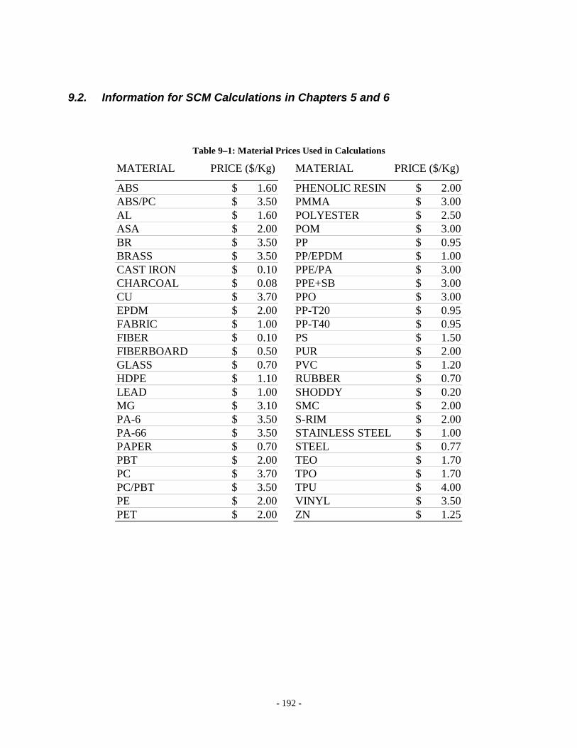
- 192 -

9.2. Information for SCM Calculations in Chapters 5 and 6

Table 9–1: Material Prices Used in Calculations

MATERIAL PRICE ($/Kg) MATERIAL PRICE ($/Kg)

ABS $ 1.60 PHENOLIC RESIN $ 2.00 ABS/PC $ 3.50 PMMA $ 3.00 AL $ 1.60 POLYESTER $ 2.50 ASA $ 2.00 POM $ 3.00 BR $ 3.50 PP $ 0.95 BRASS $ 3.50 PP/EPDM $ 1.00 CAST IRON $ 0.10 PPE/PA $ 3.00 CHARCOAL $ 0.08 PPE+SB $ 3.00 CU $ 3.70 PPO $ 3.00 EPDM $ 2.00 PP-T20 $ 0.95 FABRIC $ 1.00 PP-T40 $ 0.95 FIBER $ 0.10 PS $ 1.50 FIBERBOARD $ 0.50 PUR $ 2.00 GLASS $ 0.70 PVC $ 1.20 HDPE $ 1.10 RUBBER $ 0.70 LEAD $ 1.00 SHODDY $ 0.20 MG $ 3.10 SMC $ 2.00 PA-6 $ 3.50 S-RIM $ 2.00 PA-66 $ 3.50 STAINLESS STEEL $ 1.00 PAPER $ 0.70 STEEL $ 0.77 PBT $ 2.00 TEO $ 1.70 PC $ 3.70 TPO $ 1.70 PC/PBT $ 3.50 TPU $ 4.00 PE $ 2.00 VINYL $ 3.50 PET $ 2.00 ZN $ 1.25

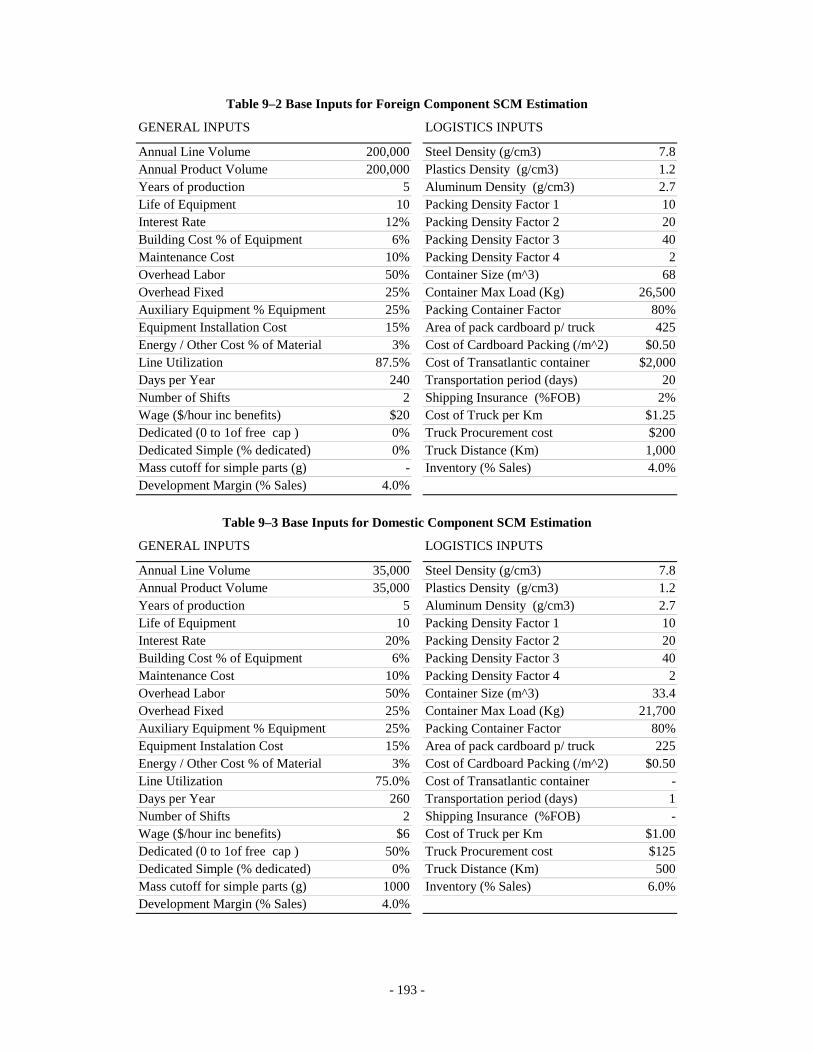
- 193 -

Table 9–2 Base Inputs for Foreign Component SCM Estimation

GENERAL INPUTS LOGISTICS INPUTS

Annual Line Volume 200,000 Steel Density (g/cm3) 7.8 Annual Product Volume 200,000 Plastics Density (g/cm3) 1.2 Years of production 5 Aluminum Density (g/cm3) 2.7 Life of Equipment 10 Packing Density Factor 1 10 Interest Rate 12% Packing Density Factor 2 20 Building Cost % of Equipment 6% Packing Density Factor 3 40 Maintenance Cost 10% Packing Density Factor 4 2 Overhead Labor 50% Container Size (m^3) 68 Overhead Fixed 25% Container Max Load (Kg) 26,500 Auxiliary Equipment % Equipment 25% Packing Container Factor 80% Equipment Installation Cost 15% Area of pack cardboard p/ truck 425 Energy / Other Cost % of Material 3% Cost of Cardboard Packing (/m^2) $0.50 Line Utilization 87.5% Cost of Transatlantic container $2,000 Days per Year 240 Transportation period (days) 20 Number of Shifts 2 Shipping Insurance (%FOB) 2% Wage ($/hour inc benefits) $20 Cost of Truck per Km $1.25 Dedicated (0 to 1of free cap ) 0% Truck Procurement cost $200 Dedicated Simple (% dedicated) 0% Truck Distance (Km) 1,000 Mass cutoff for simple parts (g) - Inventory (% Sales) 4.0% Development Margin (% Sales) 4.0%

Table 9–3 Base Inputs for Domestic Component SCM Estimation

GENERAL INPUTS LOGISTICS INPUTS

Annual Line Volume 35,000 Steel Density (g/cm3) 7.8 Annual Product Volume 35,000 Plastics Density (g/cm3) 1.2 Years of production 5 Aluminum Density (g/cm3) 2.7 Life of Equipment 10 Packing Density Factor 1 10 Interest Rate 20% Packing Density Factor 2 20 Building Cost % of Equipment 6% Packing Density Factor 3 40 Maintenance Cost 10% Packing Density Factor 4 2 Overhead Labor 50% Container Size (m^3) 33.4 Overhead Fixed 25% Container Max Load (Kg) 21,700 Auxiliary Equipment % Equipment 25% Packing Container Factor 80% Equipment Instalation Cost 15% Area of pack cardboard p/ truck 225 Energy / Other Cost % of Material 3% Cost of Cardboard Packing (/m^2) $0.50 Line Utilization 75.0% Cost of Transatlantic container - Days per Year 260 Transportation period (days) 1 Number of Shifts 2 Shipping Insurance (%FOB) - Wage ($/hour inc benefits) $6 Cost of Truck per Km $1.00 Dedicated (0 to 1of free cap ) 50% Truck Procurement cost $125 Dedicated Simple (% dedicated) 0% Truck Distance (Km) 500 Mass cutoff for simple parts (g) 1000 Inventory (% Sales) 6.0% Development Margin (% Sales) 4.0%

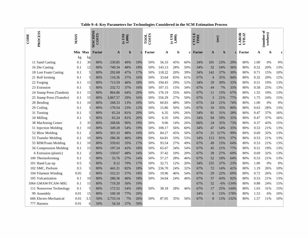
Table 9–4: Key Parameters for Technologies Considered in the SCM Estimation Process C

OD

E

PRO

CE

SS

MA

SS

MA

CH

INE

CO

STS

(x U

S$

1,00

0)

TOO

L C

OST

S

(x U

S$

1,00

0)

CY

CLE

TI

ME

(sec

)

LAB

OR

U

TILI

Z

(num

ber

of

wor

kers

)

Min Max Factor A b c Factor A b c Factor A b c Factor A b c kg kg

11 Sand Casting 0.1 30 80% 230.85 49% 19% 50% 56.33 45% 60% 34% 101 23% 29% 80% 1.00 0% 0% 16 Die Casting 0.1 12 80% 749.34 48% 18% 50% 143.13 28% 50% 34% 32 54% 36% 80% 0.52 20% 13% 18 Lost Foam Casting 0.1 5 80% 292.68 47% 17% 50% 118.22 20% 39% 34% 142 37% 30% 80% 0.71 15% 10% 21 Roll forming 0.1 5 80% 116.36 37% 16% 50% 33.64 83% 61% 67% 4 35% 84% 80% 0.32 20% 12% 22 Forging 0.1 15 80% 713.59 46% 18% 50% 194.43 29% 52% 34% 29 39% 33% 80% 0.51 19% 13% 23 Extrusion 0.1 5 80% 232.72 37% 16% 50% 107.15 15% 34% 67% 44 7% 35% 80% 0.58 25% 13% 24 Stamp Press (Tandem) 0.1 15 80% 864.86 64% 20% 50% 176.19 55% 60% 67% 11 15% 67% 80% 1.55 19% 13% 25 Stamp Press (Transfer) 0.1 15 80% 3,867.57 29% 16% 50% 556.29 27% 50% 67% 3 21% 77% 80% 1.75 24% 15% 28 Bending 0.1 10 80% 268.33 13% 10% 50% 60.83 48% 58% 67% 24 21% 74% 80% 1.00 0% 0% 29 Coiling 0.1 3 80% 170.54 23% 12% 50% 15.86 50% 54% 67% 10 35% 80% 80% 0.63 28% 13% 31 Turning 0.1 5 80% 65.24 81% 20% 50% 6.35 10% 26% 34% 81 31% 28% 80% 0.47 37% 16% 34 Milling 0.1 5 80% 65.24 81% 20% 50% 6.35 10% 26% 34% 94 59% 35% 80% 0.47 37% 16% 38 Machining Center 2 35 80% 268.66 90% 19% 50% 9.06 14% 26% 66% 24 35% 73% 80% 0.37 43% 15% 51 Injection Molding 0.1 10 80% 349.28 54% 19% 50% 108.17 56% 60% 34% 47 54% 35% 80% 0.53 21% 13% 52 Blow Molding 0.1 2 80% 301.33 48% 16% 50% 84.27 45% 50% 67% 21 117% 99% 80% 0.69 32% 13% 53 Transfer Molding 0.1 10 80% 286.36 46% 18% 50% 64.81 33% 53% 34% 113 91% 37% 80% 0.53 21% 13% 55 RIM/Foam Molding 0.1 10 80% 559.02 35% 17% 50% 93.54 27% 49% 67% 49 15% 64% 80% 0.53 21% 13% 56 Compression Molding 0.1 15 80% 197.24 42% 18% 50% 65.67 34% 54% 67% 45 21% 77% 80% 0.51 19% 13%

6 Extrusion (plastic) 0.1 2 80% 150.67 48% 16% 50% 37.42 10% 20% 67% 28 27% 69% 80% 0.69 32% 13% 100 Thermoforming 0.1 5 80% 55.76 27% 14% 50% 57.27 28% 46% 67% 52 18% 64% 80% 0.53 21% 13% 101 Hand Lay-up 0.5 5 80% 8.12 70% 17% 50% 32.71 12% 20% 34% 155 37% 23% 80% 1.00 0% 0% 102 SMC, Preform 0.5 5 80% 441.21 82% 18% 50% 236.70 24% 32% 67% 72 14% 41% 80% 1.19 26% 10% 104 Filament Winding 0.05 2 80% 552.21 57% 18% 50% 19.96 46% 54% 67% 29 22% 69% 80% 0.72 26% 13% 105 Vulcanization 0.1 10 80% 286.36 46% 18% 50% 34.64 24% 46% 67% 37 43% 92% 80% 0.53 21% 13%

1064 GMAW/FCAW-MIG 0.1 15 80% 719.20 56% 19% 67% 52 -6% -134% 80% 0.88 24% 15% 111 Nonwoven Technology 0.1 5 80% 172.52 54% 18% 50% 38.18 28% 46% 67% 17 25% 144% 80% 1.03 31% 15%

99 Assembly 0.01 15 80% 100.18 77% 20% 34% 6 15% 178% 80% 1.53 6% 10% 666 Electro-Mechanical 0.01 3.5 50% 2,733.14 7% 26% 50% 87.05 35% 56% 67% 8 13% 132% 80% 1.57 11% 10% 777 Harness 0.01 6 50% 54.34 37% 59%

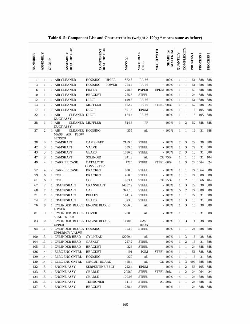
- 195 -

Table 9–5: Component List and Characteristics (weight > 100g; * means same as before)

NU

NM

BE

R

ASS

EM

BL

Y

GR

OU

P

ASS

EM

BL

Y

DE

SCR

IPT

ION

CO

MPO

NE

NT

D

ESC

RIP

TIO

N

MA

SS (g

)

MA

TE

RIA

L

TY

PE

MIX

ED

WIT

H

SHA

RE

1st

M

AT

ER

IAL

QU

AN

TIT

Y

CO

MPL

EX

ITY

PRO

CE

SS 1

PRO

CE

SS 2

PRO

CE

SS 3

1 1 1 AIR CLEANER HOUSING UPPER 572.8 PA-66 - 100% 1 1 51 888 888 3 1 1 AIR CLEANER HOUSING LOWER 754.4 PA-66 - 100% 1 1 51 888 888 6 1 1 AIR CLEANER FILTER 228.6 PAPER EPDM 100% 1 1 50 888 888

10 1 1 AIR CLEANER BRACKET 255.8 STEEL - 100% 1 1 24 888 888 12 1 1 AIR CLEANER DUCT 149.6 PA-66 - 100% 1 1 51 888 888 13 1 1 AIR CLEANER MUFFLER 862.2 PA-66 STEEL 60% 1 1 52 888 24 17 1 1 AIR CLEANER DUCT 501.8 EPDM - 100% 1 1 6 105 888 22 1 1 AIR CLEANER

DUCT ASSY DUCT 174.4 PA-66 - 100% 1 1 6 105 888

28 1 1 AIR CLEANER DUCT ASSY

MUFFLER 514.6 PP - 100% 1 2 52 888 888

37 2 1 AIR CLEANER MASS AIR FLOW SENSOR

HOUSING 355 AL - 100% 1 1 16 31 888

38 3 1 CAMSHAFT CAMSHAFT 2169.6 STEEL - 100% 2 3 22 38 888 42 3 1 CAMSHAFT VALVE 339.6 STEEL - 100% 1 3 22 31 888 43 3 1 CAMSHAFT GEARS 1036.5 STEEL - 100% 2 3 18 31 888 47 3 1 CAMSHAFT SOLINOID 341.8 AL CU 75% 1 1 16 31 104 49 4 2 CARRIER CASE CATALYTIC

CONVERTER 7720 STEEL STEEL 60% 1 3 24 1064 24

52 4 2 CARRIER CASE BRACKET 600.8 STEEL - 100% 1 1 24 1064 888 59 6 1 COIL BRACKET 460.6 STEEL - 100% 1 1 24 888 888 61 6 1 COIL COIL 983.4 STEEL CU 75% 1 2 18 666 104 67 7 1 CRANKSHAFT CRANSHAFT 14857.2 STEEL - 100% 1 3 22 38 888 68 7 1 CRANKSHAFT CAP 347.16 STEEL - 100% 5 2 24 888 888 71 7 1 CRANKSHAFT PULLEY 1441.2 STEEL - 100% 1 1 22 31 888 74 7 1 CRANKSHAFT GEARS 323.6 STEEL - 100% 1 3 18 31 888 76 8 1 CYLINDER BLOCK

LOWER ENGINE BLOCK 5566.6 AL - 100% 1 3 16 38 888

81 9 1 CYLINDER BLOCK SEAL REAR

COVER 208.6 AL - 100% 1 1 16 31 888

83 10 1 CYLINDER BLOCK UPPER

ENGINE BLOCK 33800 CAST IRON

- 100% 1 3 11 38 888

94 11 1 CYLINDER BLOCK UPPERPCV VALVE

HOUSING 353.8 STEEL - 100% 1 1 24 888 888

100 13 1 CYLINDER HEAD CYL HEAD 12209.4 AL - 100% 1 3 16 38 888 104 13 1 CYLINDER HEAD GASKET 227.2 STEEL - 100% 1 2 18 31 888 105 13 1 CYLINDER HEAD BRACKET 326 STEEL - 100% 1 1 24 888 888 126 14 1 ELEC ENG CNTRL BRACKET 101 POM STEEL 100% 1 1 51 888 888 129 14 1 ELEC ENG CNTRL HOUSING 229 AL - 100% 1 1 16 31 888 130 14 1 ELEC ENG CNTRL CIRCUIT BOARD 458.4 AL CU 100% 1 3 999 888 888 132 15 1 ENGINE ASSY SERPENTINE BELT 222.4 EPDM - 100% 1 2 56 105 888 133 15 1 ENGINE ASSY CRADLE 20560 STEEL STEEL 50% 1 2 24 1064 24 134 15 1 ENGINE ASSY CRADLE 170.05 STEEL - 100% 4 1 24 888 888 135 15 1 ENGINE ASSY TENSIONER 311.6 STEEL AL 50% 1 1 24 888 16 137 15 1 ENGINE ASSY BRACKET 738.4 STEEL - 100% 1 1 24 888 888

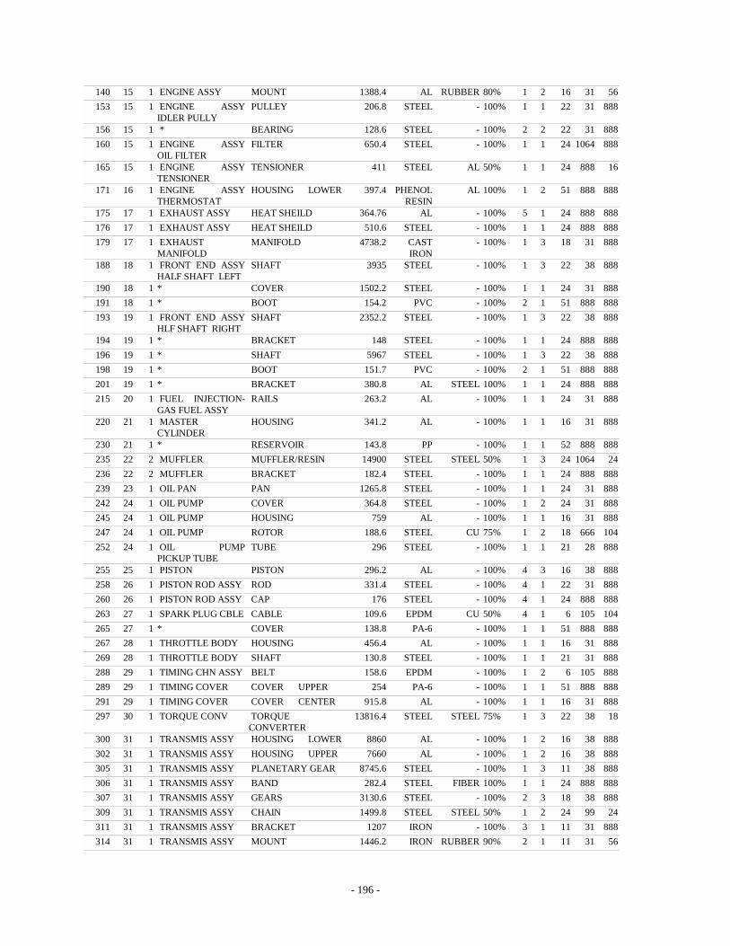
- 196 -

140 15 1 ENGINE ASSY MOUNT 1388.4 AL RUBBER 80% 1 2 16 31 56 153 15 1 ENGINE ASSY

IDLER PULLY PULLEY 206.8 STEEL - 100% 1 1 22 31 888

156 15 1 * BEARING 128.6 STEEL - 100% 2 2 22 31 888 160 15 1 ENGINE ASSY

OIL FILTER FILTER 650.4 STEEL - 100% 1 1 24 1064 888

165 15 1 ENGINE ASSY TENSIONER

TENSIONER 411 STEEL AL 50% 1 1 24 888 16

171 16 1 ENGINE ASSY THERMOSTAT

HOUSING LOWER 397.4 PHENOL RESIN

AL 100% 1 2 51 888 888

175 17 1 EXHAUST ASSY HEAT SHEILD 364.76 AL - 100% 5 1 24 888 888 176 17 1 EXHAUST ASSY HEAT SHEILD 510.6 STEEL - 100% 1 1 24 888 888 179 17 1 EXHAUST

MANIFOLD MANIFOLD 4738.2 CAST

IRON - 100% 1 3 18 31 888

188 18 1 FRONT END ASSY HALF SHAFT LEFT

SHAFT 3935 STEEL - 100% 1 3 22 38 888

190 18 1 * COVER 1502.2 STEEL - 100% 1 1 24 31 888 191 18 1 * BOOT 154.2 PVC - 100% 2 1 51 888 888 193 19 1 FRONT END ASSY

HLF SHAFT RIGHT SHAFT 2352.2 STEEL - 100% 1 3 22 38 888

194 19 1 * BRACKET 148 STEEL - 100% 1 1 24 888 888 196 19 1 * SHAFT 5967 STEEL - 100% 1 3 22 38 888 198 19 1 * BOOT 151.7 PVC - 100% 2 1 51 888 888 201 19 1 * BRACKET 380.8 AL STEEL 100% 1 1 24 888 888 215 20 1 FUEL INJECTION-

GAS FUEL ASSY RAILS 263.2 AL - 100% 1 1 24 31 888

220 21 1 MASTER CYLINDER

HOUSING 341.2 AL - 100% 1 1 16 31 888

230 21 1 * RESERVOIR 143.8 PP - 100% 1 1 52 888 888 235 22 2 MUFFLER MUFFLER/RESIN 14900 STEEL STEEL 50% 1 3 24 1064 24 236 22 2 MUFFLER BRACKET 182.4 STEEL - 100% 1 1 24 888 888 239 23 1 OIL PAN PAN 1265.8 STEEL - 100% 1 1 24 31 888 242 24 1 OIL PUMP COVER 364.8 STEEL - 100% 1 2 24 31 888 245 24 1 OIL PUMP HOUSING 759 AL - 100% 1 1 16 31 888 247 24 1 OIL PUMP ROTOR 188.6 STEEL CU 75% 1 2 18 666 104 252 24 1 OIL PUMP

PICKUP TUBE TUBE 296 STEEL - 100% 1 1 21 28 888

255 25 1 PISTON PISTON 296.2 AL - 100% 4 3 16 38 888 258 26 1 PISTON ROD ASSY ROD 331.4 STEEL - 100% 4 1 22 31 888 260 26 1 PISTON ROD ASSY CAP 176 STEEL - 100% 4 1 24 888 888 263 27 1 SPARK PLUG CBLE CABLE 109.6 EPDM CU 50% 4 1 6 105 104 265 27 1 * COVER 138.8 PA-6 - 100% 1 1 51 888 888 267 28 1 THROTTLE BODY HOUSING 456.4 AL - 100% 1 1 16 31 888 269 28 1 THROTTLE BODY SHAFT 130.8 STEEL - 100% 1 1 21 31 888 288 29 1 TIMING CHN ASSY BELT 158.6 EPDM - 100% 1 2 6 105 888 289 29 1 TIMING COVER COVER UPPER 254 PA-6 - 100% 1 1 51 888 888 291 29 1 TIMING COVER COVER CENTER 915.8 AL - 100% 1 1 16 31 888 297 30 1 TORQUE CONV TORQUE

CONVERTER 13816.4 STEEL STEEL 75% 1 3 22 38 18

300 31 1 TRANSMIS ASSY HOUSING LOWER 8860 AL - 100% 1 2 16 38 888 302 31 1 TRANSMIS ASSY HOUSING UPPER 7660 AL - 100% 1 2 16 38 888 305 31 1 TRANSMIS ASSY PLANETARY GEAR 8745.6 STEEL - 100% 1 3 11 38 888 306 31 1 TRANSMIS ASSY BAND 282.4 STEEL FIBER 100% 1 1 24 888 888 307 31 1 TRANSMIS ASSY GEARS 3130.6 STEEL - 100% 2 3 18 38 888 309 31 1 TRANSMIS ASSY CHAIN 1499.8 STEEL STEEL 50% 1 2 24 99 24 311 31 1 TRANSMIS ASSY BRACKET 1207 IRON - 100% 3 1 11 31 888 314 31 1 TRANSMIS ASSY MOUNT 1446.2 IRON RUBBER 90% 2 1 11 31 56

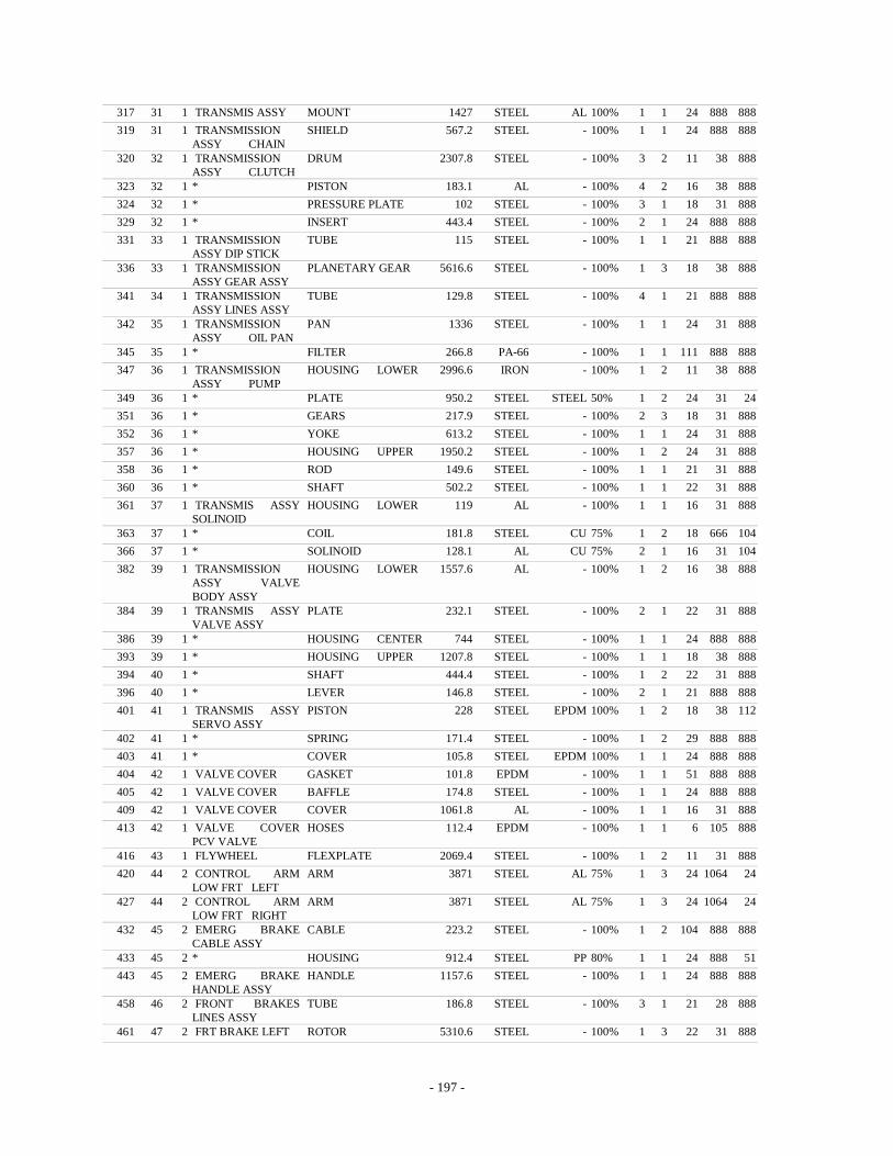
- 197 -

317 31 1 TRANSMIS ASSY MOUNT 1427 STEEL AL 100% 1 1 24 888 888 319 31 1 TRANSMISSION

ASSY CHAIN SHIELD 567.2 STEEL - 100% 1 1 24 888 888

320 32 1 TRANSMISSION ASSY CLUTCH

DRUM 2307.8 STEEL - 100% 3 2 11 38 888

323 32 1 * PISTON 183.1 AL - 100% 4 2 16 38 888 324 32 1 * PRESSURE PLATE 102 STEEL - 100% 3 1 18 31 888 329 32 1 * INSERT 443.4 STEEL - 100% 2 1 24 888 888 331 33 1 TRANSMISSION

ASSY DIP STICK TUBE 115 STEEL - 100% 1 1 21 888 888

336 33 1 TRANSMISSION ASSY GEAR ASSY

PLANETARY GEAR 5616.6 STEEL - 100% 1 3 18 38 888

341 34 1 TRANSMISSION ASSY LINES ASSY

TUBE 129.8 STEEL - 100% 4 1 21 888 888

342 35 1 TRANSMISSION ASSY OIL PAN

PAN 1336 STEEL - 100% 1 1 24 31 888

345 35 1 * FILTER 266.8 PA-66 - 100% 1 1 111 888 888 347 36 1 TRANSMISSION

ASSY PUMP HOUSING LOWER 2996.6 IRON - 100% 1 2 11 38 888

349 36 1 * PLATE 950.2 STEEL STEEL 50% 1 2 24 31 24 351 36 1 * GEARS 217.9 STEEL - 100% 2 3 18 31 888 352 36 1 * YOKE 613.2 STEEL - 100% 1 1 24 31 888 357 36 1 * HOUSING UPPER 1950.2 STEEL - 100% 1 2 24 31 888 358 36 1 * ROD 149.6 STEEL - 100% 1 1 21 31 888 360 36 1 * SHAFT 502.2 STEEL - 100% 1 1 22 31 888 361 37 1 TRANSMIS ASSY

SOLINOID HOUSING LOWER 119 AL - 100% 1 1 16 31 888

363 37 1 * COIL 181.8 STEEL CU 75% 1 2 18 666 104 366 37 1 * SOLINOID 128.1 AL CU 75% 2 1 16 31 104 382 39 1 TRANSMISSION

ASSY VALVE BODY ASSY

HOUSING LOWER 1557.6 AL - 100% 1 2 16 38 888

384 39 1 TRANSMIS ASSY VALVE ASSY

PLATE 232.1 STEEL - 100% 2 1 22 31 888

386 39 1 * HOUSING CENTER 744 STEEL - 100% 1 1 24 888 888 393 39 1 * HOUSING UPPER 1207.8 STEEL - 100% 1 1 18 38 888 394 40 1 * SHAFT 444.4 STEEL - 100% 1 2 22 31 888 396 40 1 * LEVER 146.8 STEEL - 100% 2 1 21 888 888 401 41 1 TRANSMIS ASSY

SERVO ASSY PISTON 228 STEEL EPDM 100% 1 2 18 38 112

402 41 1 * SPRING 171.4 STEEL - 100% 1 2 29 888 888 403 41 1 * COVER 105.8 STEEL EPDM 100% 1 1 24 888 888 404 42 1 VALVE COVER GASKET 101.8 EPDM - 100% 1 1 51 888 888 405 42 1 VALVE COVER BAFFLE 174.8 STEEL - 100% 1 1 24 888 888 409 42 1 VALVE COVER COVER 1061.8 AL - 100% 1 1 16 31 888 413 42 1 VALVE COVER

PCV VALVE HOSES 112.4 EPDM - 100% 1 1 6 105 888

416 43 1 FLYWHEEL FLEXPLATE 2069.4 STEEL - 100% 1 2 11 31 888 420 44 2 CONTROL ARM

LOW FRT LEFT ARM 3871 STEEL AL 75% 1 3 24 1064 24

427 44 2 CONTROL ARM LOW FRT RIGHT

ARM 3871 STEEL AL 75% 1 3 24 1064 24

432 45 2 EMERG BRAKE CABLE ASSY

CABLE 223.2 STEEL - 100% 1 2 104 888 888

433 45 2 * HOUSING 912.4 STEEL PP 80% 1 1 24 888 51 443 45 2 EMERG BRAKE

HANDLE ASSY HANDLE 1157.6 STEEL - 100% 1 1 24 888 888

458 46 2 FRONT BRAKES LINES ASSY

TUBE 186.8 STEEL - 100% 3 1 21 28 888

461 47 2 FRT BRAKE LEFT ROTOR 5310.6 STEEL - 100% 1 3 22 31 888

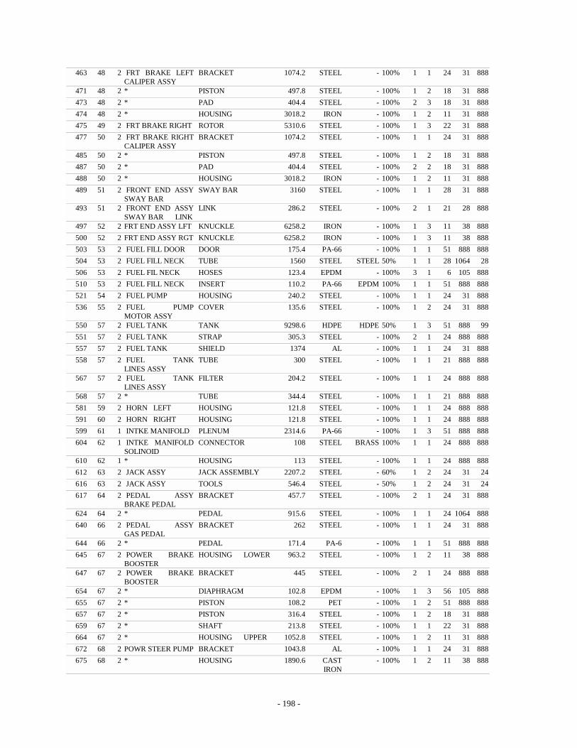
- 198 -

463 48 2 FRT BRAKE LEFT CALIPER ASSY

BRACKET 1074.2 STEEL - 100% 1 1 24 31 888

471 48 2 * PISTON 497.8 STEEL - 100% 1 2 18 31 888 473 48 2 * PAD 404.4 STEEL - 100% 2 3 18 31 888 474 48 2 * HOUSING 3018.2 IRON - 100% 1 2 11 31 888 475 49 2 FRT BRAKE RIGHT ROTOR 5310.6 STEEL - 100% 1 3 22 31 888 477 50 2 FRT BRAKE RIGHT

CALIPER ASSY BRACKET 1074.2 STEEL - 100% 1 1 24 31 888

485 50 2 * PISTON 497.8 STEEL - 100% 1 2 18 31 888 487 50 2 * PAD 404.4 STEEL - 100% 2 2 18 31 888 488 50 2 * HOUSING 3018.2 IRON - 100% 1 2 11 31 888 489 51 2 FRONT END ASSY

SWAY BAR SWAY BAR 3160 STEEL - 100% 1 1 28 31 888

493 51 2 FRONT END ASSY SWAY BAR LINK

LINK 286.2 STEEL - 100% 2 1 21 28 888

497 52 2 FRT END ASSY LFT KNUCKLE 6258.2 IRON - 100% 1 3 11 38 888 500 52 2 FRT END ASSY RGT KNUCKLE 6258.2 IRON - 100% 1 3 11 38 888 503 53 2 FUEL FILL DOOR DOOR 175.4 PA-66 - 100% 1 1 51 888 888 504 53 2 FUEL FILL NECK TUBE 1560 STEEL STEEL 50% 1 1 28 1064 28 506 53 2 FUEL FIL NECK HOSES 123.4 EPDM - 100% 3 1 6 105 888 510 53 2 FUEL FILL NECK INSERT 110.2 PA-66 EPDM 100% 1 1 51 888 888 521 54 2 FUEL PUMP HOUSING 240.2 STEEL - 100% 1 1 24 31 888 536 55 2 FUEL PUMP

MOTOR ASSY COVER 135.6 STEEL - 100% 1 2 24 31 888

550 57 2 FUEL TANK TANK 9298.6 HDPE HDPE 50% 1 3 51 888 99 551 57 2 FUEL TANK STRAP 305.3 STEEL - 100% 2 1 24 888 888 557 57 2 FUEL TANK SHIELD 1374 AL - 100% 1 1 24 31 888 558 57 2 FUEL TANK

LINES ASSY TUBE 300 STEEL - 100% 1 1 21 888 888

567 57 2 FUEL TANK LINES ASSY

FILTER 204.2 STEEL - 100% 1 1 24 888 888

568 57 2 * TUBE 344.4 STEEL - 100% 1 1 21 888 888 581 59 2 HORN LEFT HOUSING 121.8 STEEL - 100% 1 1 24 888 888 591 60 2 HORN RIGHT HOUSING 121.8 STEEL - 100% 1 1 24 888 888 599 61 1 INTKE MANIFOLD PLENUM 2314.6 PA-66 - 100% 1 3 51 888 888 604 62 1 INTKE MANIFOLD

SOLINOID CONNECTOR 108 STEEL BRASS 100% 1 1 24 888 888

610 62 1 * HOUSING 113 STEEL - 100% 1 1 24 888 888 612 63 2 JACK ASSY JACK ASSEMBLY 2207.2 STEEL - 60% 1 2 24 31 24 616 63 2 JACK ASSY TOOLS 546.4 STEEL - 50% 1 2 24 31 24 617 64 2 PEDAL ASSY

BRAKE PEDAL BRACKET 457.7 STEEL - 100% 2 1 24 31 888

624 64 2 * PEDAL 915.6 STEEL - 100% 1 1 24 1064 888 640 66 2 PEDAL ASSY

GAS PEDAL BRACKET 262 STEEL - 100% 1 1 24 31 888

644 66 2 * PEDAL 171.4 PA-6 - 100% 1 1 51 888 888 645 67 2 POWER BRAKE

BOOSTER HOUSING LOWER 963.2 STEEL - 100% 1 2 11 38 888

647 67 2 POWER BRAKE BOOSTER

BRACKET 445 STEEL - 100% 2 1 24 888 888

654 67 2 * DIAPHRAGM 102.8 EPDM - 100% 1 3 56 105 888 655 67 2 * PISTON 108.2 PET - 100% 1 2 51 888 888 657 67 2 * PISTON 316.4 STEEL - 100% 1 2 18 31 888 659 67 2 * SHAFT 213.8 STEEL - 100% 1 1 22 31 888 664 67 2 * HOUSING UPPER 1052.8 STEEL - 100% 1 2 11 31 888 672 68 2 POWR STEER PUMP BRACKET 1043.8 AL - 100% 1 1 24 31 888 675 68 2 * HOUSING 1890.6 CAST

IRON - 100% 1 2 11 38 888

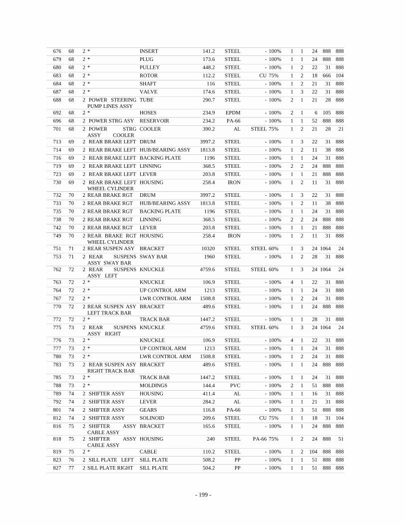
- 199 -

676 68 2 * INSERT 141.2 STEEL - 100% 1 1 24 888 888 679 68 2 * PLUG 173.6 STEEL - 100% 1 1 24 888 888 680 68 2 * PULLEY 448.2 STEEL - 100% 1 2 22 31 888 683 68 2 * ROTOR 112.2 STEEL CU 75% 1 2 18 666 104 684 68 2 * SHAFT 116 STEEL - 100% 1 2 21 31 888 687 68 2 * VALVE 174.6 STEEL - 100% 1 3 22 31 888 688 68 2 POWER STEERING

PUMP LINES ASSY TUBE 290.7 STEEL - 100% 2 1 21 28 888

692 68 2 * HOSES 234.9 EPDM - 100% 2 1 6 105 888 696 68 2 POWER STRG ASY RESERVOIR 234.2 PA-66 - 100% 1 1 52 888 888 701 68 2 POWER STRG

ASSY COOLER COOLER 390.2 AL STEEL 75% 1 2 21 28 21

713 69 2 REAR BRAKE LEFT DRUM 3997.2 STEEL - 100% 1 3 22 31 888 714 69 2 REAR BRAKE LEFT HUB/BEARING ASSY 1813.8 STEEL - 100% 1 2 11 38 888 716 69 2 REAR BRAKE LEFT BACKING PLATE 1196 STEEL - 100% 1 1 24 31 888 719 69 2 REAR BRAKE LEFT LINNING 368.5 STEEL - 100% 2 2 24 888 888 723 69 2 REAR BRAKE LEFT LEVER 203.8 STEEL - 100% 1 1 21 888 888 730 69 2 REAR BRAKE LEFT

WHEEL CYLINDER HOUSING 258.4 IRON - 100% 1 2 11 31 888

732 70 2 REAR BRAKE RGT DRUM 3997.2 STEEL - 100% 1 3 22 31 888 733 70 2 REAR BRAKE RGT HUB/BEARING ASSY 1813.8 STEEL - 100% 1 2 11 38 888 735 70 2 REAR BRAKE RGT BACKING PLATE 1196 STEEL - 100% 1 1 24 31 888 738 70 2 REAR BRAKE RGT LINNING 368.5 STEEL - 100% 2 2 24 888 888 742 70 2 REAR BRAKE RGT LEVER 203.8 STEEL - 100% 1 1 21 888 888 749 70 2 REAR BRAKE RGT

WHEEL CYLINDER HOUSING 258.4 IRON - 100% 1 2 11 31 888

751 71 2 REAR SUSPEN ASY BRACKET 10320 STEEL STEEL 60% 1 3 24 1064 24 753 71 2 REAR SUSPENS

ASSY SWAY BAR SWAY BAR 1960 STEEL - 100% 1 2 28 31 888

762 72 2 REAR SUSPENS ASSY LEFT

KNUCKLE 4759.6 STEEL STEEL 60% 1 3 24 1064 24

763 72 2 * KNUCKLE 106.9 STEEL - 100% 4 1 22 31 888 764 72 2 * UP CONTROL ARM 1213 STEEL - 100% 1 1 24 31 888 767 72 2 * LWR CONTROL ARM 1508.8 STEEL - 100% 1 2 24 31 888 770 72 2 REAR SUSPEN ASY

LEFT TRACK BAR BRACKET 489.6 STEEL - 100% 1 1 24 888 888

772 72 2 * TRACK BAR 1447.2 STEEL - 100% 1 1 28 31 888 775 73 2 REAR SUSPENS

ASSY RIGHT KNUCKLE 4759.6 STEEL STEEL 60% 1 3 24 1064 24

776 73 2 * KNUCKLE 106.9 STEEL - 100% 4 1 22 31 888 777 73 2 * UP CONTROL ARM 1213 STEEL - 100% 1 1 24 31 888 780 73 2 * LWR CONTROL ARM 1508.8 STEEL - 100% 1 2 24 31 888 783 73 2 REAR SUSPEN ASY

RIGHT TRACK BAR BRACKET 489.6 STEEL - 100% 1 1 24 888 888

785 73 2 * TRACK BAR 1447.2 STEEL - 100% 1 1 24 31 888 788 73 2 * MOLDINGS 144.4 PVC - 100% 2 1 51 888 888 789 74 2 SHIFTER ASSY HOUSING 411.4 AL - 100% 1 1 16 31 888 792 74 2 SHIFTER ASSY LEVER 284.2 AL - 100% 1 1 21 31 888 801 74 2 SHIFTER ASSY GEARS 116.8 PA-66 - 100% 1 3 51 888 888 812 74 2 SHIFTER ASSY SOLINOID 209.6 STEEL CU 75% 1 1 18 31 104 816 75 2 SHIFTER ASSY

CABLE ASSY BRACKET 165.6 STEEL - 100% 1 1 24 888 888

818 75 2 SHIFTER ASSY CABLE ASSY

HOUSING 240 STEEL PA-66 75% 1 2 24 888 51

819 75 2 * CABLE 110.2 STEEL - 100% 1 2 104 888 888 823 76 2 SILL PLATE LEFT SILL PLATE 508.2 PP - 100% 1 1 51 888 888 827 77 2 SILL PLATE RIGHT SILL PLATE 504.2 PP - 100% 1 1 51 888 888

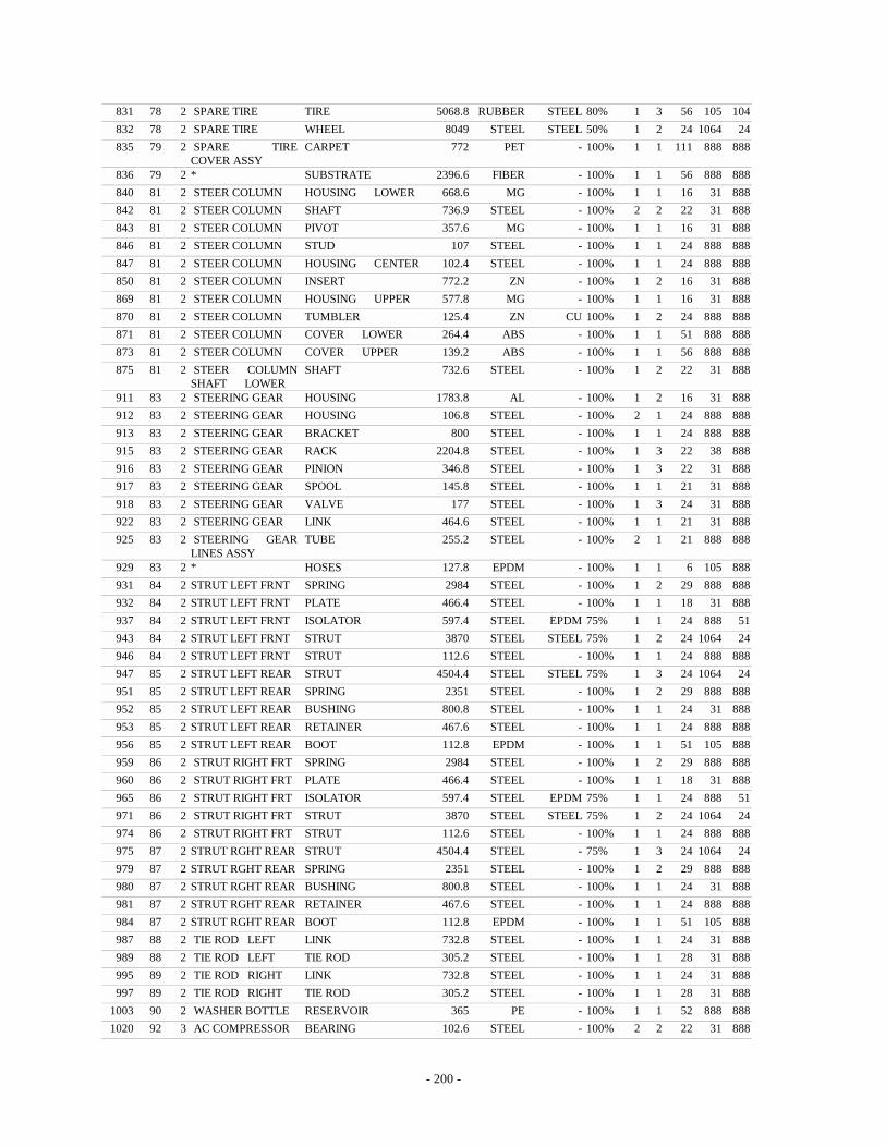
- 200 -

831 78 2 SPARE TIRE TIRE 5068.8 RUBBER STEEL 80% 1 3 56 105 104 832 78 2 SPARE TIRE WHEEL 8049 STEEL STEEL 50% 1 2 24 1064 24 835 79 2 SPARE TIRE

COVER ASSY CARPET 772 PET - 100% 1 1 111 888 888

836 79 2 * SUBSTRATE 2396.6 FIBER - 100% 1 1 56 888 888 840 81 2 STEER COLUMN HOUSING LOWER 668.6 MG - 100% 1 1 16 31 888 842 81 2 STEER COLUMN SHAFT 736.9 STEEL - 100% 2 2 22 31 888 843 81 2 STEER COLUMN PIVOT 357.6 MG - 100% 1 1 16 31 888 846 81 2 STEER COLUMN STUD 107 STEEL - 100% 1 1 24 888 888 847 81 2 STEER COLUMN HOUSING CENTER 102.4 STEEL - 100% 1 1 24 888 888 850 81 2 STEER COLUMN INSERT 772.2 ZN - 100% 1 2 16 31 888 869 81 2 STEER COLUMN HOUSING UPPER 577.8 MG - 100% 1 1 16 31 888 870 81 2 STEER COLUMN TUMBLER 125.4 ZN CU 100% 1 2 24 888 888 871 81 2 STEER COLUMN COVER LOWER 264.4 ABS - 100% 1 1 51 888 888 873 81 2 STEER COLUMN COVER UPPER 139.2 ABS - 100% 1 1 56 888 888 875 81 2 STEER COLUMN

SHAFT LOWER SHAFT 732.6 STEEL - 100% 1 2 22 31 888

911 83 2 STEERING GEAR HOUSING 1783.8 AL - 100% 1 2 16 31 888 912 83 2 STEERING GEAR HOUSING 106.8 STEEL - 100% 2 1 24 888 888 913 83 2 STEERING GEAR BRACKET 800 STEEL - 100% 1 1 24 888 888 915 83 2 STEERING GEAR RACK 2204.8 STEEL - 100% 1 3 22 38 888 916 83 2 STEERING GEAR PINION 346.8 STEEL - 100% 1 3 22 31 888 917 83 2 STEERING GEAR SPOOL 145.8 STEEL - 100% 1 1 21 31 888 918 83 2 STEERING GEAR VALVE 177 STEEL - 100% 1 3 24 31 888 922 83 2 STEERING GEAR LINK 464.6 STEEL - 100% 1 1 21 31 888 925 83 2 STEERING GEAR

LINES ASSY TUBE 255.2 STEEL - 100% 2 1 21 888 888

929 83 2 * HOSES 127.8 EPDM - 100% 1 1 6 105 888 931 84 2 STRUT LEFT FRNT SPRING 2984 STEEL - 100% 1 2 29 888 888 932 84 2 STRUT LEFT FRNT PLATE 466.4 STEEL - 100% 1 1 18 31 888 937 84 2 STRUT LEFT FRNT ISOLATOR 597.4 STEEL EPDM 75% 1 1 24 888 51 943 84 2 STRUT LEFT FRNT STRUT 3870 STEEL STEEL 75% 1 2 24 1064 24 946 84 2 STRUT LEFT FRNT STRUT 112.6 STEEL - 100% 1 1 24 888 888 947 85 2 STRUT LEFT REAR STRUT 4504.4 STEEL STEEL 75% 1 3 24 1064 24 951 85 2 STRUT LEFT REAR SPRING 2351 STEEL - 100% 1 2 29 888 888 952 85 2 STRUT LEFT REAR BUSHING 800.8 STEEL - 100% 1 1 24 31 888 953 85 2 STRUT LEFT REAR RETAINER 467.6 STEEL - 100% 1 1 24 888 888 956 85 2 STRUT LEFT REAR BOOT 112.8 EPDM - 100% 1 1 51 105 888 959 86 2 STRUT RIGHT FRT SPRING 2984 STEEL - 100% 1 2 29 888 888 960 86 2 STRUT RIGHT FRT PLATE 466.4 STEEL - 100% 1 1 18 31 888 965 86 2 STRUT RIGHT FRT ISOLATOR 597.4 STEEL EPDM 75% 1 1 24 888 51 971 86 2 STRUT RIGHT FRT STRUT 3870 STEEL STEEL 75% 1 2 24 1064 24 974 86 2 STRUT RIGHT FRT STRUT 112.6 STEEL - 100% 1 1 24 888 888 975 87 2 STRUT RGHT REAR STRUT 4504.4 STEEL - 75% 1 3 24 1064 24 979 87 2 STRUT RGHT REAR SPRING 2351 STEEL - 100% 1 2 29 888 888 980 87 2 STRUT RGHT REAR BUSHING 800.8 STEEL - 100% 1 1 24 31 888 981 87 2 STRUT RGHT REAR RETAINER 467.6 STEEL - 100% 1 1 24 888 888 984 87 2 STRUT RGHT REAR BOOT 112.8 EPDM - 100% 1 1 51 105 888 987 88 2 TIE ROD LEFT LINK 732.8 STEEL - 100% 1 1 24 31 888 989 88 2 TIE ROD LEFT TIE ROD 305.2 STEEL - 100% 1 1 28 31 888 995 89 2 TIE ROD RIGHT LINK 732.8 STEEL - 100% 1 1 24 31 888 997 89 2 TIE ROD RIGHT TIE ROD 305.2 STEEL - 100% 1 1 28 31 888

1003 90 2 WASHER BOTTLE RESERVOIR 365 PE - 100% 1 1 52 888 888 1020 92 3 AC COMPRESSOR BEARING 102.6 STEEL - 100% 2 2 22 31 888

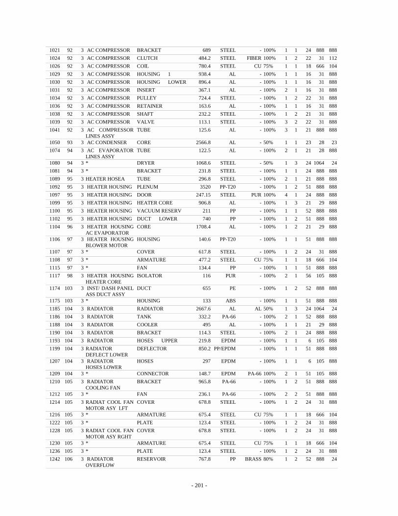
- 201 -

1021 92 3 AC COMPRESSOR BRACKET 689 STEEL - 100% 1 1 24 888 888 1024 92 3 AC COMPRESSOR CLUTCH 484.2 STEEL FIBER 100% 1 2 22 31 112 1026 92 3 AC COMPRESSOR COIL 780.4 STEEL CU 75% 1 1 18 666 104 1029 92 3 AC COMPRESSOR HOUSING 1 938.4 AL - 100% 1 1 16 31 888 1030 92 3 AC COMPRESSOR HOUSING LOWER 896.4 AL - 100% 1 1 16 31 888 1031 92 3 AC COMPRESSOR INSERT 367.1 AL - 100% 2 1 16 31 888 1034 92 3 AC COMPRESSOR PULLEY 724.4 STEEL - 100% 1 2 22 31 888 1036 92 3 AC COMPRESSOR RETAINER 163.6 AL - 100% 1 1 16 31 888 1038 92 3 AC COMPRESSOR SHAFT 232.2 STEEL - 100% 1 2 21 31 888 1039 92 3 AC COMPRESSOR VALVE 113.1 STEEL - 100% 3 2 22 31 888 1041 92 3 AC COMPRESSOR

LINES ASSY TUBE 125.6 AL - 100% 3 1 21 888 888

1050 93 3 AC CONDENSER CORE 2566.8 AL - 50% 1 1 23 28 23 1074 94 3 AC EVAPORATOR

LINES ASSY TUBE 122.5 AL - 100% 2 1 21 28 888

1080 94 3 * DRYER 1068.6 STEEL - 50% 1 3 24 1064 24 1081 94 3 * BRACKET 231.8 STEEL - 100% 1 1 24 888 888 1089 95 3 HEATER HOSEA TUBE 296.8 STEEL - 100% 2 1 21 888 888 1092 95 3 HEATER HOUSING PLENUM 3520 PP-T20 - 100% 1 2 51 888 888 1097 95 3 HEATER HOUSING DOOR 247.15 STEEL PUR 100% 4 1 24 888 888 1099 95 3 HEATER HOUSING HEATER CORE 906.8 AL - 100% 1 3 21 29 888 1100 95 3 HEATER HOUSING VACUUM RESERV 211 PP - 100% 1 1 52 888 888 1102 95 3 HEATER HOUSING DUCT LOWER 740 PP - 100% 1 2 51 888 888 1104 96 3 HEATER HOUSING

AC EVAPORATOR CORE 1708.4 AL - 100% 1 2 21 29 888

1106 97 3 HEATER HOUSING BLOWER MOTOR

HOUSING 140.6 PP-T20 - 100% 1 1 51 888 888

1107 97 3 * COVER 617.8 STEEL - 100% 1 2 24 31 888 1108 97 3 * ARMATURE 477.2 STEEL CU 75% 1 1 18 666 104 1115 97 3 * FAN 134.4 PP - 100% 1 1 51 888 888 1117 98 3 HEATER HOUSING

HEATER CORE ISOLATOR 116 PUR - 100% 2 1 56 105 888

1174 103 3 INST/ DASH PANEL ASS DUCT ASSY

DUCT 655 PE - 100% 1 2 52 888 888

1175 103 3 * HOUSING 133 ABS - 100% 1 1 51 888 888 1185 104 3 RADIATOR RADIATOR 2667.6 AL AL 50% 1 3 24 1064 24 1186 104 3 RADIATOR TANK 332.2 PA-66 - 100% 2 1 52 888 888 1188 104 3 RADIATOR COOLER 495 AL - 100% 1 1 21 29 888 1190 104 3 RADIATOR BRACKET 114.3 STEEL - 100% 2 1 24 888 888 1193 104 3 RADIATOR HOSES UPPER 219.8 EPDM - 100% 1 1 6 105 888 1199 104 3 RADIATOR

DEFLECT LOWER DEFLECTOR 850.2 PP/EPDM - 100% 1 1 51 888 888

1207 104 3 RADIATOR HOSES LOWER

HOSES 297 EPDM - 100% 1 1 6 105 888

1209 104 3 * CONNECTOR 148.7 EPDM PA-66 100% 2 1 51 105 888 1210 105 3 RADIATOR

COOLING FAN BRACKET 965.8 PA-66 - 100% 1 2 51 888 888

1212 105 3 * FAN 236.1 PA-66 - 100% 2 2 51 888 888 1214 105 3 RADIAT COOL FAN

MOTOR ASY LFT COVER 678.8 STEEL - 100% 1 2 24 31 888

1216 105 3 * ARMATURE 675.4 STEEL CU 75% 1 1 18 666 104 1222 105 3 * PLATE 123.4 STEEL - 100% 1 2 24 31 888 1228 105 3 RADIAT COOL FAN

MOTOR ASY RGHT COVER 678.8 STEEL - 100% 1 2 24 31 888

1230 105 3 * ARMATURE 675.4 STEEL CU 75% 1 1 18 666 104 1236 105 3 * PLATE 123.4 STEEL - 100% 1 2 24 31 888 1242 106 3 RADIATOR

OVERFLOW RESERVOIR 767.8 PP BRASS 80% 1 2 52 888 24

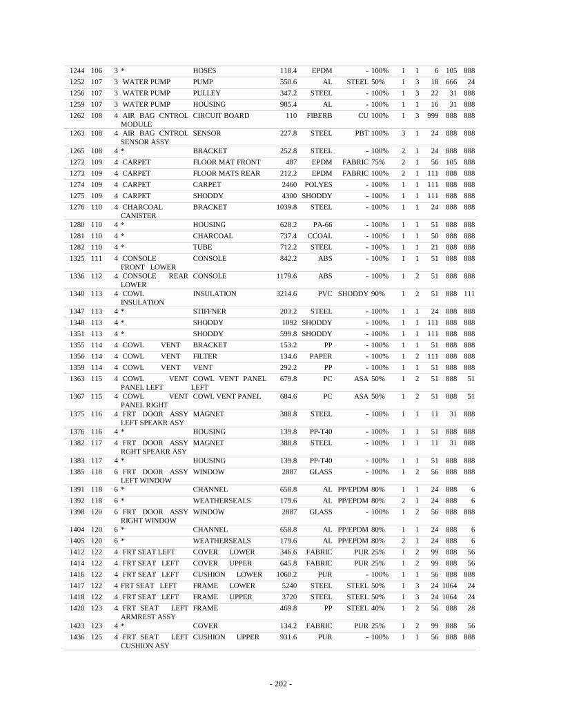
- 202 -

1244 106 3 * HOSES 118.4 EPDM - 100% 1 1 6 105 888 1252 107 3 WATER PUMP PUMP 550.6 AL STEEL 50% 1 3 18 666 24 1256 107 3 WATER PUMP PULLEY 347.2 STEEL - 100% 1 3 22 31 888 1259 107 3 WATER PUMP HOUSING 985.4 AL - 100% 1 1 16 31 888 1262 108 4 AIR BAG CNTROL

MODULE CIRCUIT BOARD 110 FIBERB CU 100% 1 3 999 888 888

1263 108 4 AIR BAG CNTROL SENSOR ASSY

SENSOR 227.8 STEEL PBT 100% 3 1 24 888 888

1265 108 4 * BRACKET 252.8 STEEL - 100% 2 1 24 888 888 1272 109 4 CARPET FLOOR MAT FRONT 487 EPDM FABRIC 75% 2 1 56 105 888 1273 109 4 CARPET FLOOR MATS REAR 212.2 EPDM FABRIC 100% 2 1 111 888 888 1274 109 4 CARPET CARPET 2460 POLYES - 100% 1 1 111 888 888 1275 109 4 CARPET SHODDY 4300 SHODDY - 100% 1 1 111 888 888 1276 110 4 CHARCOAL

CANISTER BRACKET 1039.8 STEEL - 100% 1 1 24 888 888

1280 110 4 * HOUSING 628.2 PA-66 - 100% 1 1 51 888 888 1281 110 4 * CHARCOAL 737.4 CCOAL - 100% 1 1 50 888 888 1282 110 4 * TUBE 712.2 STEEL - 100% 1 1 21 888 888 1325 111 4 CONSOLE

FRONT LOWER CONSOLE 842.2 ABS - 100% 1 1 51 888 888

1336 112 4 CONSOLE REAR LOWER

CONSOLE 1179.6 ABS - 100% 1 2 51 888 888

1340 113 4 COWL INSULATION

INSULATION 3214.6 PVC SHODDY 90% 1 2 51 888 111

1347 113 4 * STIFFNER 203.2 STEEL - 100% 1 1 24 888 888 1348 113 4 * SHODDY 1092 SHODDY - 100% 1 1 111 888 888 1351 113 4 * SHODDY 599.8 SHODDY - 100% 1 1 111 888 888 1355 114 4 COWL VENT BRACKET 153.2 PP - 100% 1 1 51 888 888 1356 114 4 COWL VENT FILTER 134.6 PAPER - 100% 1 2 111 888 888 1359 114 4 COWL VENT VENT 292.2 PP - 100% 1 1 51 888 888 1363 115 4 COWL VENT

PANEL LEFT COWL VENT PANEL LEFT

679.8 PC ASA 50% 1 2 51 888 51

1367 115 4 COWL VENT PANEL RIGHT

COWL VENT PANEL 684.6 PC ASA 50% 1 2 51 888 51

1375 116 4 FRT DOOR ASSY LEFT SPEAKR ASY

MAGNET 388.8 STEEL - 100% 1 1 11 31 888

1376 116 4 * HOUSING 139.8 PP-T40 - 100% 1 1 51 888 888 1382 117 4 FRT DOOR ASSY

RGHT SPEAKR ASY MAGNET 388.8 STEEL - 100% 1 1 11 31 888

1383 117 4 * HOUSING 139.8 PP-T40 - 100% 1 1 51 888 888 1385 118 6 FRT DOOR ASSY

LEFT WINDOW WINDOW 2887 GLASS - 100% 1 2 56 888 888

1391 118 6 * CHANNEL 658.8 AL PP/EPDM 80% 1 1 24 888 6 1392 118 6 * WEATHERSEALS 179.6 AL PP/EPDM 80% 2 1 24 888 6 1398 120 6 FRT DOOR ASSY

RIGHT WINDOW WINDOW 2887 GLASS - 100% 1 2 56 888 888

1404 120 6 * CHANNEL 658.8 AL PP/EPDM 80% 1 1 24 888 6 1405 120 6 * WEATHERSEALS 179.6 AL PP/EPDM 80% 2 1 24 888 6 1412 122 4 FRT SEAT LEFT COVER LOWER 346.6 FABRIC PUR 25% 1 2 99 888 56 1414 122 4 FRT SEAT LEFT COVER UPPER 645.8 FABRIC PUR 25% 1 2 99 888 56 1416 122 4 FRT SEAT LEFT CUSHION LOWER 1060.2 PUR - 100% 1 1 56 888 888 1417 122 4 FRT SEAT LEFT FRAME LOWER 5240 STEEL STEEL 50% 1 3 24 1064 24 1418 122 4 FRT SEAT LEFT FRAME UPPER 3720 STEEL STEEL 50% 1 3 24 1064 24 1420 123 4 FRT SEAT LEFT

ARMREST ASSY FRAME 469.8 PP STEEL 40% 1 2 56 888 28

1423 123 4 * COVER 134.2 FABRIC PUR 25% 1 2 99 888 56 1436 125 4 FRT SEAT LEFT

CUSHION ASY CUSHION UPPER 931.6 PUR - 100% 1 1 56 888 888

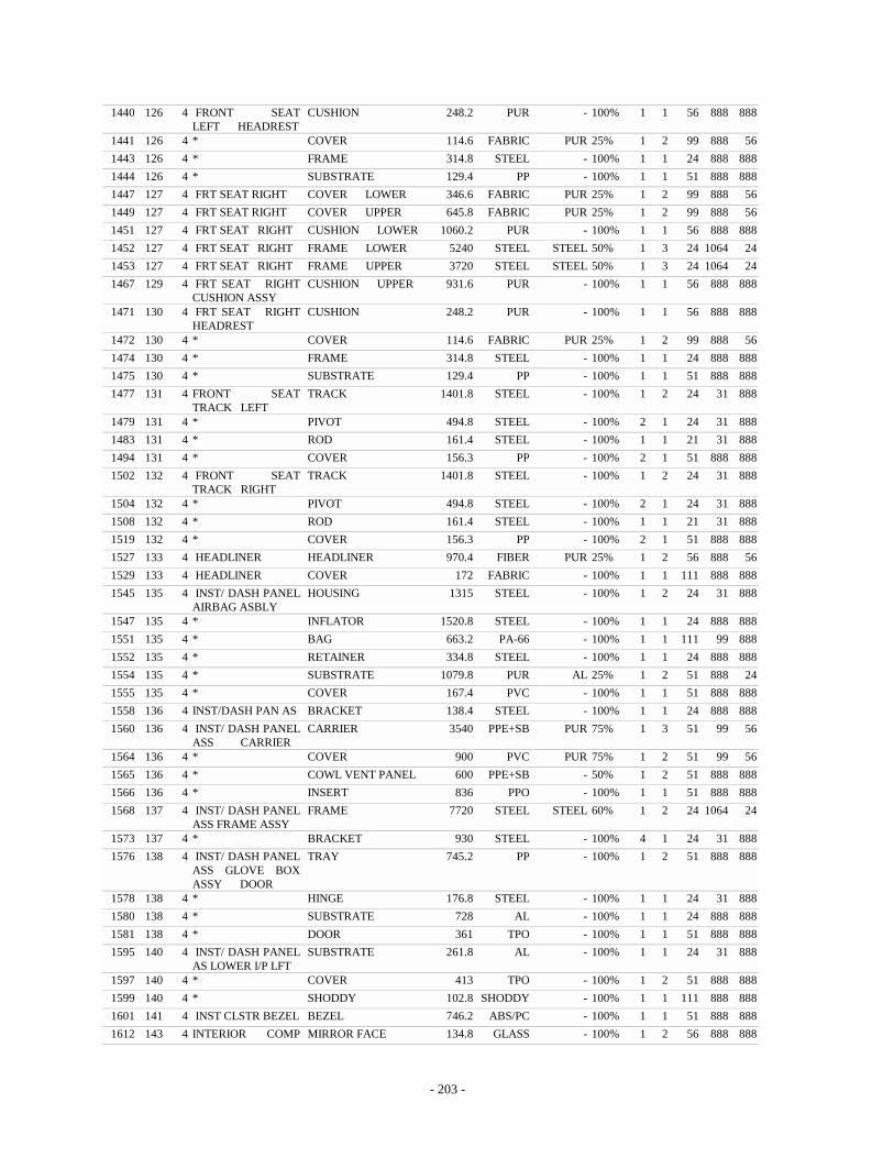
- 203 -

1440 126 4 FRONT SEAT LEFT HEADREST

CUSHION 248.2 PUR - 100% 1 1 56 888 888

1441 126 4 * COVER 114.6 FABRIC PUR 25% 1 2 99 888 56 1443 126 4 * FRAME 314.8 STEEL - 100% 1 1 24 888 888 1444 126 4 * SUBSTRATE 129.4 PP - 100% 1 1 51 888 888 1447 127 4 FRT SEAT RIGHT COVER LOWER 346.6 FABRIC PUR 25% 1 2 99 888 56 1449 127 4 FRT SEAT RIGHT COVER UPPER 645.8 FABRIC PUR 25% 1 2 99 888 56 1451 127 4 FRT SEAT RIGHT CUSHION LOWER 1060.2 PUR - 100% 1 1 56 888 888 1452 127 4 FRT SEAT RIGHT FRAME LOWER 5240 STEEL STEEL 50% 1 3 24 1064 24 1453 127 4 FRT SEAT RIGHT FRAME UPPER 3720 STEEL STEEL 50% 1 3 24 1064 24 1467 129 4 FRT SEAT RIGHT

CUSHION ASSY CUSHION UPPER 931.6 PUR - 100% 1 1 56 888 888

1471 130 4 FRT SEAT RIGHT HEADREST

CUSHION 248.2 PUR - 100% 1 1 56 888 888

1472 130 4 * COVER 114.6 FABRIC PUR 25% 1 2 99 888 56 1474 130 4 * FRAME 314.8 STEEL - 100% 1 1 24 888 888 1475 130 4 * SUBSTRATE 129.4 PP - 100% 1 1 51 888 888 1477 131 4 FRONT SEAT

TRACK LEFT TRACK 1401.8 STEEL - 100% 1 2 24 31 888

1479 131 4 * PIVOT 494.8 STEEL - 100% 2 1 24 31 888 1483 131 4 * ROD 161.4 STEEL - 100% 1 1 21 31 888 1494 131 4 * COVER 156.3 PP - 100% 2 1 51 888 888 1502 132 4 FRONT SEAT

TRACK RIGHT TRACK 1401.8 STEEL - 100% 1 2 24 31 888

1504 132 4 * PIVOT 494.8 STEEL - 100% 2 1 24 31 888 1508 132 4 * ROD 161.4 STEEL - 100% 1 1 21 31 888 1519 132 4 * COVER 156.3 PP - 100% 2 1 51 888 888 1527 133 4 HEADLINER HEADLINER 970.4 FIBER PUR 25% 1 2 56 888 56 1529 133 4 HEADLINER COVER 172 FABRIC - 100% 1 1 111 888 888 1545 135 4 INST/ DASH PANEL

AIRBAG ASBLY HOUSING 1315 STEEL - 100% 1 2 24 31 888

1547 135 4 * INFLATOR 1520.8 STEEL - 100% 1 1 24 888 888 1551 135 4 * BAG 663.2 PA-66 - 100% 1 1 111 99 888 1552 135 4 * RETAINER 334.8 STEEL - 100% 1 1 24 888 888 1554 135 4 * SUBSTRATE 1079.8 PUR AL 25% 1 2 51 888 24 1555 135 4 * COVER 167.4 PVC - 100% 1 1 51 888 888 1558 136 4 INST/DASH PAN AS BRACKET 138.4 STEEL - 100% 1 1 24 888 888 1560 136 4 INST/ DASH PANEL

ASS CARRIER CARRIER 3540 PPE+SB PUR 75% 1 3 51 99 56

1564 136 4 * COVER 900 PVC PUR 75% 1 2 51 99 56 1565 136 4 * COWL VENT PANEL 600 PPE+SB - 50% 1 2 51 888 888 1566 136 4 * INSERT 836 PPO - 100% 1 1 51 888 888 1568 137 4 INST/ DASH PANEL

ASS FRAME ASSY FRAME 7720 STEEL STEEL 60% 1 2 24 1064 24

1573 137 4 * BRACKET 930 STEEL - 100% 4 1 24 31 888 1576 138 4 INST/ DASH PANEL

ASS GLOVE BOX ASSY DOOR

TRAY 745.2 PP - 100% 1 2 51 888 888

1578 138 4 * HINGE 176.8 STEEL - 100% 1 1 24 31 888 1580 138 4 * SUBSTRATE 728 AL - 100% 1 1 24 888 888 1581 138 4 * DOOR 361 TPO - 100% 1 1 51 888 888 1595 140 4 INST/ DASH PANEL

AS LOWER I/P LFT SUBSTRATE 261.8 AL - 100% 1 1 24 31 888

1597 140 4 * COVER 413 TPO - 100% 1 2 51 888 888 1599 140 4 * SHODDY 102.8 SHODDY - 100% 1 1 111 888 888 1601 141 4 INST CLSTR BEZEL BEZEL 746.2 ABS/PC - 100% 1 1 51 888 888 1612 143 4 INTERIOR COMP

REAR MIRROR MIRROR FACE 134.8 GLASS - 100% 1 2 56 888 888

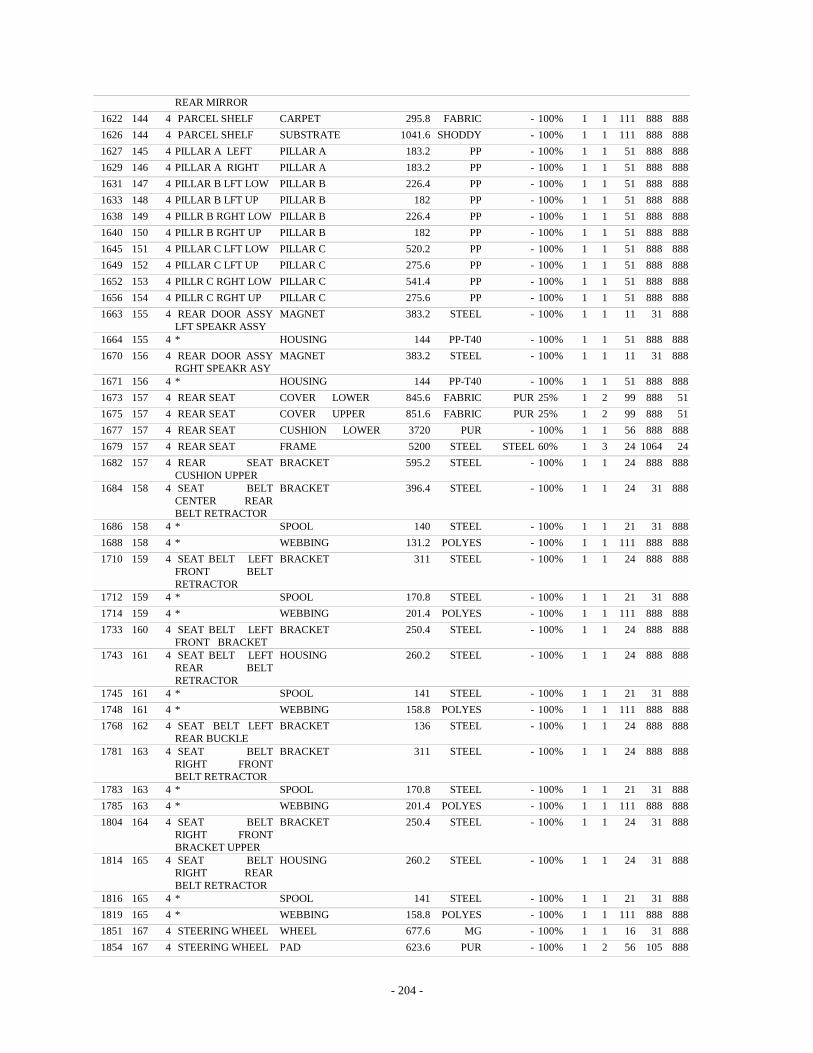
- 204 -

REAR MIRROR 1622 144 4 PARCEL SHELF CARPET 295.8 FABRIC - 100% 1 1 111 888 888 1626 144 4 PARCEL SHELF SUBSTRATE 1041.6 SHODDY - 100% 1 1 111 888 888 1627 145 4 PILLAR A LEFT PILLAR A 183.2 PP - 100% 1 1 51 888 888 1629 146 4 PILLAR A RIGHT PILLAR A 183.2 PP - 100% 1 1 51 888 888 1631 147 4 PILLAR B LFT LOW PILLAR B 226.4 PP - 100% 1 1 51 888 888 1633 148 4 PILLAR B LFT UP PILLAR B 182 PP - 100% 1 1 51 888 888 1638 149 4 PILLR B RGHT LOW PILLAR B 226.4 PP - 100% 1 1 51 888 888 1640 150 4 PILLR B RGHT UP PILLAR B 182 PP - 100% 1 1 51 888 888 1645 151 4 PILLAR C LFT LOW PILLAR C 520.2 PP - 100% 1 1 51 888 888 1649 152 4 PILLAR C LFT UP PILLAR C 275.6 PP - 100% 1 1 51 888 888 1652 153 4 PILLR C RGHT LOW PILLAR C 541.4 PP - 100% 1 1 51 888 888 1656 154 4 PILLR C RGHT UP PILLAR C 275.6 PP - 100% 1 1 51 888 888 1663 155 4 REAR DOOR ASSY

LFT SPEAKR ASSY MAGNET 383.2 STEEL - 100% 1 1 11 31 888

1664 155 4 * HOUSING 144 PP-T40 - 100% 1 1 51 888 888 1670 156 4 REAR DOOR ASSY

RGHT SPEAKR ASY MAGNET 383.2 STEEL - 100% 1 1 11 31 888

1671 156 4 * HOUSING 144 PP-T40 - 100% 1 1 51 888 888 1673 157 4 REAR SEAT COVER LOWER 845.6 FABRIC PUR 25% 1 2 99 888 51 1675 157 4 REAR SEAT COVER UPPER 851.6 FABRIC PUR 25% 1 2 99 888 51 1677 157 4 REAR SEAT CUSHION LOWER 3720 PUR - 100% 1 1 56 888 888 1679 157 4 REAR SEAT FRAME 5200 STEEL STEEL 60% 1 3 24 1064 24 1682 157 4 REAR SEAT

CUSHION UPPER BRACKET 595.2 STEEL - 100% 1 1 24 888 888

1684 158 4 SEAT BELT CENTER REAR BELT RETRACTOR

BRACKET 396.4 STEEL - 100% 1 1 24 31 888

1686 158 4 * SPOOL 140 STEEL - 100% 1 1 21 31 888 1688 158 4 * WEBBING 131.2 POLYES - 100% 1 1 111 888 888 1710 159 4 SEAT BELT LEFT

FRONT BELT RETRACTOR

BRACKET 311 STEEL - 100% 1 1 24 888 888

1712 159 4 * SPOOL 170.8 STEEL - 100% 1 1 21 31 888 1714 159 4 * WEBBING 201.4 POLYES - 100% 1 1 111 888 888 1733 160 4 SEAT BELT LEFT

FRONT BRACKET BRACKET 250.4 STEEL - 100% 1 1 24 888 888

1743 161 4 SEAT BELT LEFT REAR BELT RETRACTOR

HOUSING 260.2 STEEL - 100% 1 1 24 888 888

1745 161 4 * SPOOL 141 STEEL - 100% 1 1 21 31 888 1748 161 4 * WEBBING 158.8 POLYES - 100% 1 1 111 888 888 1768 162 4 SEAT BELT LEFT

REAR BUCKLE BRACKET 136 STEEL - 100% 1 1 24 888 888

1781 163 4 SEAT BELT RIGHT FRONT BELT RETRACTOR

BRACKET 311 STEEL - 100% 1 1 24 888 888

1783 163 4 * SPOOL 170.8 STEEL - 100% 1 1 21 31 888 1785 163 4 * WEBBING 201.4 POLYES - 100% 1 1 111 888 888 1804 164 4 SEAT BELT

RIGHT FRONT BRACKET UPPER

BRACKET 250.4 STEEL - 100% 1 1 24 31 888

1814 165 4 SEAT BELT RIGHT REAR BELT RETRACTOR

HOUSING 260.2 STEEL - 100% 1 1 24 31 888

1816 165 4 * SPOOL 141 STEEL - 100% 1 1 21 31 888 1819 165 4 * WEBBING 158.8 POLYES - 100% 1 1 111 888 888 1851 167 4 STEERING WHEEL WHEEL 677.6 MG - 100% 1 1 16 31 888 1854 167 4 STEERING WHEEL PAD 623.6 PUR - 100% 1 2 56 105 888

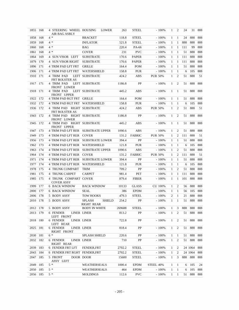
- 205 -

1855 168 4 STEERING WHEEL AIR BAG ASBLY

HOUSING LOWER 263 STEEL - 100% 1 2 24 31 888

1858 168 4 * BRACKET 118.8 STEEL - 100% 1 1 24 888 888 1859 168 4 * INFLATOR 521.8 STEEL - 100% 1 1 888 888 888 1860 168 4 * BAG 220.4 PA-66 - 100% 1 1 111 99 888 1861 168 4 * COVER 231 PVC - 100% 1 1 51 888 888 1864 169 4 SUN VISOR LEFT SUBSTRATE 170.6 PAPER - 100% 1 1 111 888 888 1879 170 4 SUN VISOR RIGHT SUBSTRATE 170.6 PAPER - 100% 1 1 111 888 888 1896 171 4 TRIM PAD LFT FRT GRILLE 164.4 POM - 100% 1 1 51 888 888 1906 171 4 TRIM PAD LFT FRT WATERSHIELD 158.8 PUR - 100% 1 1 6 105 888 1910 171 4 TRIM PAD LEFT

FRT BOLSTER AS SUBSTRATE 424.2 ABS PUR 50% 1 2 51 888 51

1917 171 4 TRIM PAD LEFT FRONT LOWER

SUBSTRATE 1186.8 PP - 100% 1 2 51 888 888

1918 171 4 TRIM PAD LEFT FRONT UPPER

SUBSTRATE 445.2 ABS - 100% 1 1 51 888 888

1922 172 4 TRIM PAD RGT FRT GRILLE 164.4 POM - 100% 1 1 51 888 888 1932 172 4 TRIM PAD RGT FRT WATERSHIELD 158.8 PUR - 100% 1 1 6 105 888 1936 172 4 TRIM PAD RIGHT

FRT BOLSTER AS SUBSTRATE 424.2 ABS PUR 50% 1 2 51 888 51

1943 172 4 TRIM PAD RIGHT FRONT LOWER

SUBSTRATE 1186.8 PP - 100% 1 2 51 888 888

1945 172 4 TRIM PAD RIGHT FRONT UPPER

SUBSTRATE 445.2 ABS - 100% 1 1 51 888 888

1947 173 4 TRIM PAD LFT RER SUBSTRATE UPPER 1090.6 ABS - 100% 1 2 51 888 888 1949 173 4 TRIM PAD LFT RER COVER 131.2 FABRIC PUR 50% 1 2 111 888 51 1956 173 4 TRIM PAD LFT RER SUBSTRATE LOWER 394.4 PP - 100% 1 1 51 888 888 1962 173 4 TRIM PAD LFT RER WATERSHIELD 121.8 PUR - 100% 1 1 6 105 888 1963 174 4 TRIM PAD LFT RER SUBSTRATE UPPER 1090.6 ABS - 100% 1 2 51 888 888 1964 174 4 TRIM PAD LFT RER COVER 131.2 FABRIC PUR 50% 1 2 111 888 51 1971 174 4 TRIM PAD LFT RER SUBSTRATE LOWER 394.4 PP - 100% 1 1 51 888 888 1977 174 4 TRIM PAD LFT RER WATERSHIELD 121.8 PUR - 100% 1 1 6 105 888 1978 175 4 TRUNK COMPART TRIM 709.2 PP - 100% 1 2 51 888 888 1981 175 4 TRUNK CARPET CARPET 981.4 PET - 100% 1 1 111 888 888 1985 175 4 TRUNK COMPART

COVER ASSY COVER 879.4 FIBER - 100% 1 1 101 888 888

1999 177 6 BACK WINDOW BACK WINDOW 10133 GLASS CU 100% 1 2 56 888 888 2000 177 6 BACK WINDOW SEAL 386 EPDM - 100% 1 1 56 105 888 2006 178 5 BODY ASSY TOW HOOKS 479.3 STEEL - 100% 2 1 21 888 888 2010 178 5 BODY ASSY SPLASH SHIELD

RIGHT REAR 254.2 PP - 100% 1 1 51 888 888

2012 178 5 BODY ASSY BODY IN WHITE 269688 STEEL - 100% 1 3 888 888 888 2013 179 6 FENDER LINER

LEFT FRONT LINER 813.2 PP - 100% 1 2 51 888 888

2018 180 6 FENDER LINER LEFT REAR

LINER 722.8 PP - 100% 1 2 51 888 888

2025 181 6 FENDER LINER RIGHT FRONT

LINER 818.4 PP - 100% 1 2 51 888 888

2030 181 6 * SPLASH SHIELD 220.6 PP - 100% 1 1 51 888 888 2032 182 6 FENDER LINER

RIGHT REAR LINER 710 PP - 100% 1 2 51 888 888

2039 183 6 FENDER FRT LFT FENDER,FRT 2702.2 STEEL - 100% 1 2 24 1064 888 2043 184 6 FENDER FRT RGHT FENDER,FRT 2702.2 STEEL - 100% 1 2 24 1064 888 2047 185 5 FRONT DOOR

ASSY LEFT DOOR 15600 STEEL - 100% 1 3 888 888 888

2049 185 5 * WEATHERSEALS 1000.4 EPDM STEEL 40% 1 1 6 105 24 2050 185 5 * WEATHERSEALS 464 EPDM - 100% 1 1 6 105 888 2056 185 5 * MOLDINGS 112.6 PVC - 100% 1 1 51 888 888

- 206 -

2066 187 5 FRT DOOR ASSY LEFT DOOR CHECK

DOOR CHECK 214 STEEL - 100% 1 1 24 888 888

2087 189 4 FRT DOOR ASSY LEFT LATCH ASSY

FRAME 247.6 STEEL - 100% 1 3 24 1064 888

2120 192 4 FRT DOOR ASSY LEFT REGULATOR

CHANNEL 467 STEEL - 100% 1 1 24 888 888

2137 193 5 FRONT DOOR ASSY RIGHT

DOOR 15600 STEEL - 100% 1 3 888 888 888

2139 193 5 * WEATHERSEALS 1000.4 EPDM STEEL 40% 1 1 6 105 24 2140 193 5 * WEATHERSEALS 464 EPDM - 100% 1 1 6 105 888 2146 193 5 * MOLDINGS 112.6 PVC - 100% 1 1 51 888 888 2156 195 5 FRONT DOOR

ASSY RIGHT DOOR CHECK

DOOR CHECK 214 STEEL - 100% 1 1 24 888 888

2178 197 4 FRONT DOOR ASSY RIGHT LATCH ASSY

FRAME 247.6 STEEL - 100% 1 3 24 1064 888

2211 200 4 FRT DOOR ASSY RGHT REGULATOR

CHANNEL 467 STEEL - 100% 1 1 24 888 888

2228 201 5 FRONT DOOR HINGE LEFT

HINGE 345.3 STEEL - 100% 2 1 24 31 888

2230 201 5 * HINGE 345.2 STEEL - 100% 2 1 24 31 888 2232 201 5 * HINGE 354.6 STEEL - 100% 2 1 24 31 888 2234 201 5 * HINGE 354.6 STEEL - 100% 2 1 24 31 888 2236 202 6 HOOD HOOD 14800 STEEL - 100% 1 3 24 888 888 2238 202 6 HOOD HINGE 349.2 STEEL - 100% 2 1 24 31 888 2240 202 6 HOOD ROD 330 STEEL - 100% 1 1 21 31 888 2241 202 6 HOOD WEATHERSEALS

FRONT 156.8 EPDM - 100% 1 1 6 105 888

2243 202 6 HOOD WEATHERSEALS REAR

357.2 EPDM - 100% 1 1 6 105 888

2258 204 6 HOOD LATCH ASY LATCH 454.8 STEEL - 100% 1 3 24 1064 888 2268 207 5 REAR DOOR ASSY

LEFT DOOR 12840 STEEL - 100% 1 3 888 888 888

2270 207 5 * DOOR CHECK 213 STEEL - 100% 1 1 24 888 888 2273 207 5 REAR DOOR ASSY

LEFT WEATHERSEALS 859.6 EPDM - 100% 1 1 6 105 888

2304 210 4 REAR DOOR ASSY LEFT LATCH ASSY

FRAME 274.8 STEEL - 100% 1 3 24 1064 888

2333 212 4 REAR DOOR ASSY LFT REGULATOR

CHANNEL 298.6 STEEL - 100% 1 1 24 31 888

2351 212 4 REAR DOOR ASSY LFT REGULATOR ASSY CABLE

HOUSING 120.6 STEEL PVC 100% 1 2 24 888 888

2352 213 6 REAR DOOR ASSY LEFT WINDOW

WINDOW 2497.4 GLASS - 100% 1 2 56 888 888

2355 213 6 * CHANNEL 466.4 AL PP/EPDM 80% 1 1 24 888 50 2356 213 6 * SEAL 149.3 AL PP/EPDM 100% 2 1 16 31 888 2364 215 5 REAR DOOR ASSY

RIGHT DOOR 12840 STEEL - 100% 1 3 888 888 888

2366 215 5 * DOOR CHECK 213 STEEL - 100% 1 1 24 888 888 2369 215 5 * WEATHERSEALS 859.6 EPDM - 100% 1 1 6 105 888 2400 218 4 REAR DOOR ASSY

RGHT LATCH ASSY FRAME 274.8 STEEL - 100% 1 3 24 1064 888

2429 220 4 REAR DOOR ASSY RGHT REGULATOR

CHANNEL 298.6 STEEL - 100% 1 2 24 31 888

2447 220 4 REAR DOOR ASSY RGHT REGULATOR ASSY CABLE

HOUSING 120.6 STEEL PVC 100% 1 2 24 888 888

2448 221 6 REAR DOOR ASSY RIGHT WINDOW

WINDOW 2497.4 GLASS - 100% 1 2 56 888 888

2451 221 6 * CHANNEL 466.4 AL PP/EPDM 80% 1 1 24 888 50

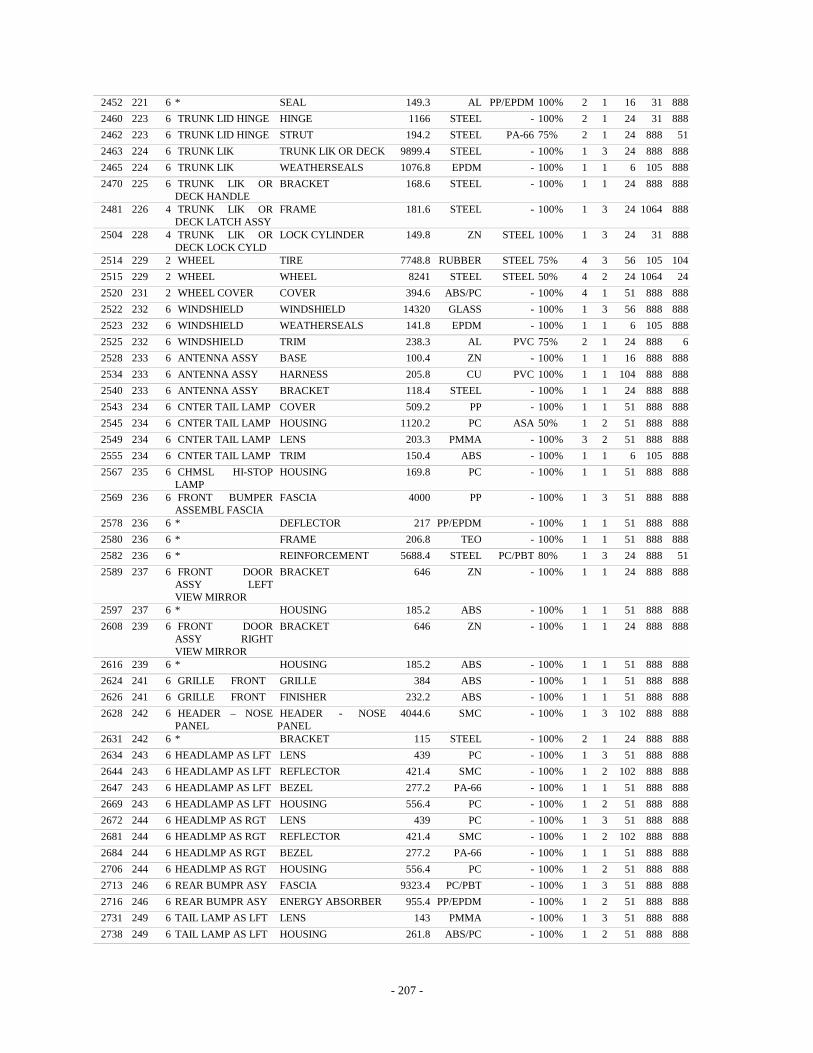
- 207 -

2452 221 6 * SEAL 149.3 AL PP/EPDM 100% 2 1 16 31 888 2460 223 6 TRUNK LID HINGE HINGE 1166 STEEL - 100% 2 1 24 31 888 2462 223 6 TRUNK LID HINGE STRUT 194.2 STEEL PA-66 75% 2 1 24 888 51 2463 224 6 TRUNK LIK TRUNK LIK OR DECK 9899.4 STEEL - 100% 1 3 24 888 888 2465 224 6 TRUNK LIK WEATHERSEALS 1076.8 EPDM - 100% 1 1 6 105 888 2470 225 6 TRUNK LIK OR

DECK HANDLE BRACKET 168.6 STEEL - 100% 1 1 24 888 888

2481 226 4 TRUNK LIK OR DECK LATCH ASSY

FRAME 181.6 STEEL - 100% 1 3 24 1064 888

2504 228 4 TRUNK LIK OR DECK LOCK CYLD

LOCK CYLINDER 149.8 ZN STEEL 100% 1 3 24 31 888

2514 229 2 WHEEL TIRE 7748.8 RUBBER STEEL 75% 4 3 56 105 104 2515 229 2 WHEEL WHEEL 8241 STEEL STEEL 50% 4 2 24 1064 24 2520 231 2 WHEEL COVER COVER 394.6 ABS/PC - 100% 4 1 51 888 888 2522 232 6 WINDSHIELD WINDSHIELD 14320 GLASS - 100% 1 3 56 888 888 2523 232 6 WINDSHIELD WEATHERSEALS 141.8 EPDM - 100% 1 1 6 105 888 2525 232 6 WINDSHIELD TRIM 238.3 AL PVC 75% 2 1 24 888 6 2528 233 6 ANTENNA ASSY BASE 100.4 ZN - 100% 1 1 16 888 888 2534 233 6 ANTENNA ASSY HARNESS 205.8 CU PVC 100% 1 1 104 888 888 2540 233 6 ANTENNA ASSY BRACKET 118.4 STEEL - 100% 1 1 24 888 888 2543 234 6 CNTER TAIL LAMP COVER 509.2 PP - 100% 1 1 51 888 888 2545 234 6 CNTER TAIL LAMP HOUSING 1120.2 PC ASA 50% 1 2 51 888 888 2549 234 6 CNTER TAIL LAMP LENS 203.3 PMMA - 100% 3 2 51 888 888 2555 234 6 CNTER TAIL LAMP TRIM 150.4 ABS - 100% 1 1 6 105 888 2567 235 6 CHMSL HI-STOP

LAMP HOUSING 169.8 PC - 100% 1 1 51 888 888

2569 236 6 FRONT BUMPER ASSEMBL FASCIA

FASCIA 4000 PP - 100% 1 3 51 888 888

2578 236 6 * DEFLECTOR 217 PP/EPDM - 100% 1 1 51 888 888 2580 236 6 * FRAME 206.8 TEO - 100% 1 1 51 888 888 2582 236 6 * REINFORCEMENT 5688.4 STEEL PC/PBT 80% 1 3 24 888 51 2589 237 6 FRONT DOOR

ASSY LEFT VIEW MIRROR

BRACKET 646 ZN - 100% 1 1 24 888 888

2597 237 6 * HOUSING 185.2 ABS - 100% 1 1 51 888 888 2608 239 6 FRONT DOOR

ASSY RIGHT VIEW MIRROR

BRACKET 646 ZN - 100% 1 1 24 888 888

2616 239 6 * HOUSING 185.2 ABS - 100% 1 1 51 888 888 2624 241 6 GRILLE FRONT GRILLE 384 ABS - 100% 1 1 51 888 888 2626 241 6 GRILLE FRONT FINISHER 232.2 ABS - 100% 1 1 51 888 888 2628 242 6 HEADER – NOSE

PANEL HEADER - NOSE PANEL

4044.6 SMC - 100% 1 3 102 888 888

2631 242 6 * BRACKET 115 STEEL - 100% 2 1 24 888 888 2634 243 6 HEADLAMP AS LFT LENS 439 PC - 100% 1 3 51 888 888 2644 243 6 HEADLAMP AS LFT REFLECTOR 421.4 SMC - 100% 1 2 102 888 888 2647 243 6 HEADLAMP AS LFT BEZEL 277.2 PA-66 - 100% 1 1 51 888 888 2669 243 6 HEADLAMP AS LFT HOUSING 556.4 PC - 100% 1 2 51 888 888 2672 244 6 HEADLMP AS RGT LENS 439 PC - 100% 1 3 51 888 888 2681 244 6 HEADLMP AS RGT REFLECTOR 421.4 SMC - 100% 1 2 102 888 888 2684 244 6 HEADLMP AS RGT BEZEL 277.2 PA-66 - 100% 1 1 51 888 888 2706 244 6 HEADLMP AS RGT HOUSING 556.4 PC - 100% 1 2 51 888 888 2713 246 6 REAR BUMPR ASY FASCIA 9323.4 PC/PBT - 100% 1 3 51 888 888 2716 246 6 REAR BUMPR ASY ENERGY ABSORBER 955.4 PP/EPDM - 100% 1 2 51 888 888 2731 249 6 TAIL LAMP AS LFT LENS 143 PMMA - 100% 1 3 51 888 888 2738 249 6 TAIL LAMP AS LFT HOUSING 261.8 ABS/PC - 100% 1 2 51 888 888

- 208 -

2740 250 6 TAIL LAMP AS RGT LENS 143 PMMA - 100% 1 3 51 888 888 2747 250 6 TAIL LAMP AS RGT HOUSING 261.8 ABS/PC - 100% 1 2 51 888 888 2749 251 6 WINDSHIELD

WIPER ARM LEFT ARM 299.8 STEEL - 100% 1 3 24 888 888

2757 251 6 * BLADE 126 STEEL - 100% 1 3 24 888 888 2761 251 6 WINDSHIELD

WIPER ARM RGHT ARM 321 STEEL - 100% 1 3 24 888 888

2769 251 6 * BLADE 126 STEEL - 100% 1 3 24 888 888 2773 252 6 WIPER MOTOR HOUSING 250.8 AL - 100% 1 1 16 31 888 2775 252 6 WIPER MOTOR ARMATURE 403.2 STEEL CU 75% 1 2 18 666 104 2789 252 6 WIPER MOTOR COVER 562 STEEL - 100% 1 1 24 888 888 2791 253 6 WIPER TRANSM BRACKET 591.5 STEEL - 100% 1 2 24 888 888 2793 253 6 WIPER TRANSM PIVOT 157.9 ZN - 100% 2 3 16 888 888 2794 253 6 WIPER TRANSM ROD 161 STEEL - 100% 2 1 21 31 888 2795 253 6 WIPER TRANSM ARM 196.8 STEEL - 100% 3 1 24 888 888 2803 254 7 CRUISE SPEED

CONTROL BRACKET 138 STEEL - 100% 1 1 24 888 888

2805 254 7 * HOUSING LOWER 221.2 AL - 100% 1 1 24 31 888 2806 254 7 * COIL 331.2 STEEL CU 80% 1 1 21 31 104 2807 254 7 * ARMATURE 118.8 STEEL - 100% 1 1 18 666 888 2808 254 7 * GEARS 133.2 STEEL - 100% 1 3 18 31 888 2828 254 7 CRUISE SPEED

BRACKET ASSY BRACKET 181.6 STEEL - 100% 1 1 24 888 888

2830 254 7 CRUISE SPEED CABLE ASSY

HOUSING 148 STEEL PA-66 100% 1 1 24 888 888

2857 257 7 INST/ DASH PANEL ASS SWITCH ASSY

HOUSING 107.2 ABS - 100% 1 1 51 888 888

2874 258 7 INSTRUMENT CLUSTER

HOUSING LOWER 437.8 PP-T20 - 100% 1 1 51 888 888

2905 260 7 INSTRUMENT CLUSTER SPEEDOM ASSY

BEZEL 168.4 ABS - 100% 1 1 51 888 888

2906 260 7 * LENS 122 PMMA - 100% 1 2 51 888 888 2910 261 7 RADIO BRACKET 403 ABS - 100% 1 1 51 888 888 2912 261 7 RADIO HOUSING 385.2 STEEL - 100% 1 1 24 888 888 2914 261 7 RADIO BRACKET 107.4 MG - 100% 1 1 24 888 888 2916 261 7 RADIO CIRCUIT BOARD 114.2 FIBER CU 100% 2 3 999 888 888 2918 261 7 RADIO HEAT SINK 102.6 ZN - 100% 1 1 24 888 888 2920 261 7 RADIO TAPE DECK 532.6 STEEL CU 100% 1 1 24 888 888 2980 268 8 ALTERNATOR HOUSING LOWER 700.4 AL - 100% 1 1 16 31 888 2982 268 8 ALTERNATOR STATOR 1368.6 STEEL CU 75% 1 3 24 888 104 2983 268 8 ALTERNATOR ROTOR 3275.6 STEEL CU 80% 1 3 11 666 104 2984 268 8 ALTERNATOR BEARING 106.4 STEEL - 100% 1 2 22 31 888 2985 268 8 ALTERNATOR CONTACT 331.8 AL CU 90% 1 3 24 888 888 2993 268 8 ALTERNATOR HOUSING UPPER 342.8 STEEL - 100% 1 1 24 888 888 2994 268 8 ALTERNATOR PULLEY 166.2 STEEL - 100% 1 1 22 31 888 2996 268 8 ALTERNATOR BRACKET 1787.4 AL - 100% 1 1 16 31 888 2998 269 8 BATTERY

COVER ASSY BATTERY 14753.2 LEAD PP 90% 1 1 16 99 51

3003 269 8 BATTERY TRAY RETAINER 161 STEEL - 100% 1 1 24 888 888 3005 269 8 BATTERY TRAY TRAY 1477.2 STEEL - 100% 1 1 24 888 888 3007 270 8 STARTER HOUSING LOWER 502.8 AL - 100% 1 1 16 31 888 3009 270 8 STARTER HOUSING CENTER 743.4 STEEL - 100% 1 1 24 31 888 3012 270 8 STARTER SHAFT 173.2 STEEL - 100% 1 1 21 31 888 3014 270 8 STARTER ARMATURE 856.8 STEEL CU 75% 1 1 18 666 104 3016 270 8 STARTER CLUTCH 231.2 STEEL - 100% 1 2 18 31 888 3022 270 8 STARTER HOLDER 183 PA-66 CU 100% 1 1 51 888 888

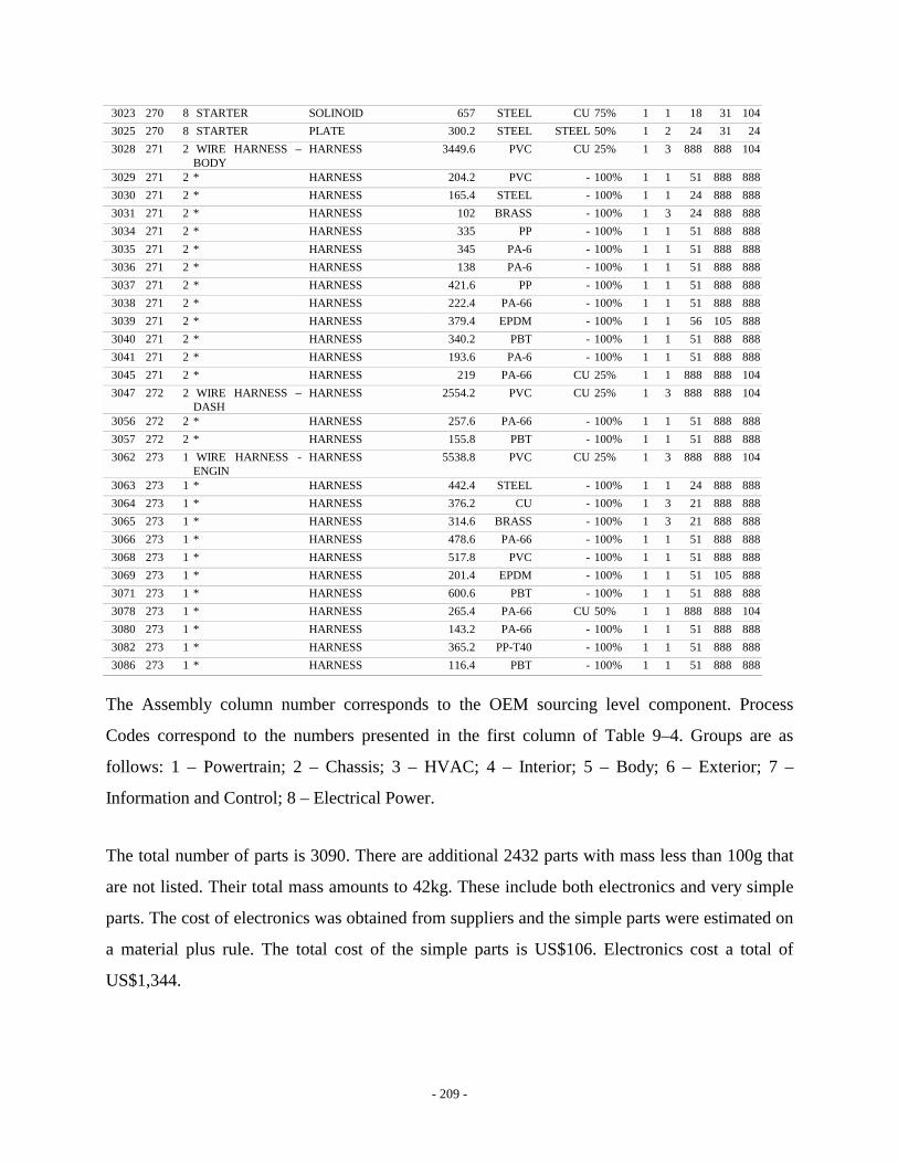
- 209 -

3023 270 8 STARTER SOLINOID 657 STEEL CU 75% 1 1 18 31 104 3025 270 8 STARTER PLATE 300.2 STEEL STEEL 50% 1 2 24 31 24 3028 271 2 WIRE HARNESS –

BODY HARNESS 3449.6 PVC CU 25% 1 3 888 888 104

3029 271 2 * HARNESS 204.2 PVC - 100% 1 1 51 888 888 3030 271 2 * HARNESS 165.4 STEEL - 100% 1 1 24 888 888 3031 271 2 * HARNESS 102 BRASS - 100% 1 3 24 888 888 3034 271 2 * HARNESS 335 PP - 100% 1 1 51 888 888 3035 271 2 * HARNESS 345 PA-6 - 100% 1 1 51 888 888 3036 271 2 * HARNESS 138 PA-6 - 100% 1 1 51 888 888 3037 271 2 * HARNESS 421.6 PP - 100% 1 1 51 888 888 3038 271 2 * HARNESS 222.4 PA-66 - 100% 1 1 51 888 888 3039 271 2 * HARNESS 379.4 EPDM - 100% 1 1 56 105 888 3040 271 2 * HARNESS 340.2 PBT - 100% 1 1 51 888 888 3041 271 2 * HARNESS 193.6 PA-6 - 100% 1 1 51 888 888 3045 271 2 * HARNESS 219 PA-66 CU 25% 1 1 888 888 104 3047 272 2 WIRE HARNESS –

DASH HARNESS 2554.2 PVC CU 25% 1 3 888 888 104

3056 272 2 * HARNESS 257.6 PA-66 - 100% 1 1 51 888 888 3057 272 2 * HARNESS 155.8 PBT - 100% 1 1 51 888 888 3062 273 1 WIRE HARNESS -

ENGIN HARNESS 5538.8 PVC CU 25% 1 3 888 888 104

3063 273 1 * HARNESS 442.4 STEEL - 100% 1 1 24 888 888 3064 273 1 * HARNESS 376.2 CU - 100% 1 3 21 888 888 3065 273 1 * HARNESS 314.6 BRASS - 100% 1 3 21 888 888 3066 273 1 * HARNESS 478.6 PA-66 - 100% 1 1 51 888 888 3068 273 1 * HARNESS 517.8 PVC - 100% 1 1 51 888 888 3069 273 1 * HARNESS 201.4 EPDM - 100% 1 1 51 105 888 3071 273 1 * HARNESS 600.6 PBT - 100% 1 1 51 888 888 3078 273 1 * HARNESS 265.4 PA-66 CU 50% 1 1 888 888 104 3080 273 1 * HARNESS 143.2 PA-66 - 100% 1 1 51 888 888 3082 273 1 * HARNESS 365.2 PP-T40 - 100% 1 1 51 888 888 3086 273 1 * HARNESS 116.4 PBT - 100% 1 1 51 888 888

The Assembly column number corresponds to the OEM sourcing level component. Process

Codes correspond to the numbers presented in the first column of Table 9–4. Groups are as

follows: 1 – Powertrain; 2 – Chassis; 3 – HVAC; 4 – Interior; 5 – Body; 6 – Exterior; 7 –

Information and Control; 8 – Electrical Power.

The total number of parts is 3090. There are additional 2432 parts with mass less than 100g that

are not listed. Their total mass amounts to 42kg. These include both electronics and very simple

parts. The cost of electronics was obtained from suppliers and the simple parts were estimated on

a material plus rule. The total cost of the simple parts is US$106. Electronics cost a total of

US$1,344.

- 210 -

References

Aghion, P. and P. Howitt (1998). Endogenous Growth Theory. Cambridge, MIT Press.

Aitken, B. J., G. H. Hanson, et al. (1997). “Spillovers, Foreign Investment, and Export Behavior.” Journal of International Economics 43(1-2): p 103-32.

Aitken, B. J. and A. E. Harrison (1999). “Do Domestic Firms Benefit from Direct Foreign Investment? Evidence from Venezuela.” American Economic Review 89(3): p 605-18.

Aitken, B. J., A. E. Harrison, et al. (1996). “Wages and Foreign Ownership: A comparative study of Mexico, Venezuela and the United States.” Journal of International Economics 40: 345-371.

Amsden, A. (1989). Asia's Next Giant: South Korea and Late Industrialization, Oxford University Press.

Amsden, A. (2000). Industrialization under new WTO law. High Level Round Table on Trade and Development: Directions for the Twenty-first Century, Bangkok.

Amsden, A. (2000). The Rise of the Rest, 1850-2000: Late industrialization outside the nort-atlantic economies, Oxford University Press.

Anderson, S. W. (1995). A Framework for Assessing Cost Management System Changes: The Case of Activity Based Costing Implementation at General Motors, 1986-1993. Cambridge, IMVP: 63.

Argote, L., S. L. Beckman, et al. (1990). “The persistence and transfer of learning in industrial settings.” Management Science 36(2): 140-154.

Arntzen, B. C., G. G. Brown, et al. (1995). “Global supply chain management at Digital Equipment Corporation.” Interfaces 25(1): 69-93.

Arrow, K. (1962). “The Economic Implications of Learning by Doing.” Review of Economic Studies 28: 155-73.

Bale, H. E. and D. A. Walters (1986). “Investment Policy Aspects of US and Global Trade Interests.” Looking Ahead 9(1): 1-14.

Ballman, P. and R. Shusman (1959). Easy Ways to Calculate Injection Molding Set-Up, Modern Plastics. NY, McGraw-Hill.

Beghin, J. C. and C. A. K. Lovell (1993). “Trade and Efficiency Effects of Domestic Content Protection: The Australian Tobacco and Cigarette Industries.” Review of Economics & Statistics 75(4): 623-31.

Belderbos, R. A. and L. Sleuwaegen (1997). “Local Content Requirements and Vertical Market Structure.” European Journal of Political Economy 13(1): 101-19.

Bell, M. P. K. (1993). “Technological Accumulation and Industrial Growth: Contrasts Between Developed and developing Countries.” Industrial and Corporate Change 2(2): 157- 210.

Bennet, D. C. and K. E. Sharpe (1990). Transnational Corporations versus the State: Political Economy of the Mexican Auto Industry. Princeton, NJ, Princeton University Press.

Bennet, M. (1986). Public Policy and Industrial Development: The Case of the Mexican Auto Parts Industry. Boulder, Colorado, Westview Press.

Berry, S., J. Levinson, et al. (1995). “Automobile Prices in Market Equilibrium.” Econometrica 63(4): 841-890.

Blomstrom, M. and A. Kokko (1998). “Multinational Corporations and Spillovers.” Journal of Economic Surveys 12(3): p 247-77.

Blomstrom, M. and H. Persson (1983). “Foreign Investment and Spillover Efficiency in an Underdeveloped Economy: Evidence from the Mexican Manufacturing Industry.” World Development 11: 493-501.

Boothroyd, G., P. Dewhurst, et al. (1994). Product design for manufacture and assembly. New York, M. Dekker.

- 211 -

Borensztein, E., J. Gregorio, et al. (1995). “How does FDI Affect Economic Growth.” NBER Working Paper Series(5057).

Brainard, S. L. and D. Martimort (1997). “Strategic trade policy with incompletely informed policymakers.” Journal of International Economics 42: 33-65.

Brander, J. and B. Spencer (1985). “Export Subsidies and International Market Share Rivlary.” JIE 18: 83-100.

Brannon, J. T., D. D. James, et al. (1994). “Generating and Sustaining Backward Linkages.” World Development 22(12): 1933-1945.

Braunerhjelm, P. and R. Svensson (1996). “Host Country Characteristics and Agglomeration in Foreign Direct Investment.” Applied Economics 28(7): p 833-40.

Brent, R. (1990). Project Appraisal for Developing Nations. New York, New York University Press.

Buckley, P. and M. Casson (1976). The Future of the Multinational Enterprise. London, MacMillan.

Busch, J. V. (1987). Technical Cost Modeling of Plastic Fabrication Processes. Materials Science and Engineering. Cambridge, MIT: 164.

Busch, J. V. and F. R. Field III (1988). Technical Cost Modeling. The Blow Molding Handbook. D. Rosato and D. Rosato. New York, Hansr Publishers. Chapter 24: 839-871.

Caves, R. (1976). Multinational Enterprise and Economic Analysis. London, Cambridge University Press.

Caves, R. (1996). Multinational Enterprise and Economic Analysis. Cambridge, Cambridge University Press.

Chitrakar, R. and J. Weiss (1995). “Foreign Investment in Nepal in the 1980s: A Cost Benefit Evaluation.” The Journal of Development Studies 31(3): p 451-66.

Chuang, Y.-C. and C.-M. Lin (1999). “Foreign Direct Investment, R&D and Spillover Efficiency: Evidence from Taiwan's Mannufacturing Firms.” Journal of Development Studies 35(4): 117-137.

Clark, J. P., R. Roth, et al., Eds. (1997). Techno-Economic Issues in Materials Selection. Materials Selection and Design. Materials Park, OH, ASM International.

Clark, J. P. and F. Veloso (2000). The vertical integration of the component supplier chains and its impact on multi-tier supplier relations. The automotive industry: Component suppliers; current and prospective regulatory approaches. Sta Maria da Feira, Portugal.

Cohen, M. and S. Mallik (1997). “Global Supply Chains: Research and Applications.” Production and Operations Management 6(3): 193-210.

Cooper, R. and P. Kaplan (1988). “Measure Costs Right.” Harvard Business Review(Sept-Oct).

Curry, S. and J. Weiss (1993). Project analysis in developing countries. New York, N.Y., St. Martin's Press.

Dahlman, C., Ross-Larson B. and L. Westphal (1985). “Managing Technological Development: Lessons from the NICs.” World Bank Staff Working Paper: 717.

Dasgupta, P. and J. Stiglitz (1988). “Learning-by-doing, market structures and industrial and trade policies.” Oxford Economic Papers 40: 246-268.

Davidson, C., S. J. Matusz, et al. (1985). “Analysis of Performance Standards for Direct Foreign Investments.” Canadian Journal of Economics 18(4): 876-90.

de Mello Jr., L. R. (1995). “Vintage Capital Accumulation: Endogenous Growth Conditions.” Journal of Macroeconomics 17: 703-716.

de Mello Jr., L. R. (1997). “Foreign Direct Investment in Developing Countries and Growth: A Selective Survey.” Journal of Development Studies 34(1): 1-34.

Dinwiddy, C. L. and F. Teal (1996). Principles of cost-benefit analysis for developing countries. Cambridge ; New York, Cambridge University Press.

- 212 -

Dunning, J. (1981). International Production and the Multinational Enterprise. London, Georoge, Allen and Unwin.

EIU (1999). European Automotive Components. London, Economist Intelligence Unit.

Fosfuri, A. and M. Motta (1999). “Multinationals without Advantages.” Scandinavian Journal of Economics 101(4): p 617-30.

Frischtak, C. (1986). Brazil. National Policies for Developing High Tech Industries: International Comparisons. F. R. a. C. Brown. Boulder, Westview Press.

Fukasaku, K. (2000). Special and Differential Treatment for Developing Countries: Does It Help Those Who Help Themselves? Globalisation and the Obstacles to the Successful Integration of Small Vulnerable Economies, Paris, UN/WIDER.

German, L. (1998). Low Volume Manufactuing Strategies for the Automotive Industry: A Global and Emerging Economy Perspective. Materials Engineering. Cambridge, Massachusetts, MIT: 119.

Gershwin, S. B. (1994). Manufacturing systems engineering. Englewood Cliffs, N.J., PTR Prentice Hall.

Global Interest Group (1998). The Globalization of the Automobile industry. Greenwich, Connecticut, Mckinsey & Co.

Gorg, H. and F. Ruane (2000). “An analysis of backward linkages in the Irish electronics.” Economic and Social Review 31(3): 215-235.

Gray, P. and I. Walter (1984). “Investment-related trade distortions in petrochemicals.” Journal of World Trade Law(January): pp. 283-307.

Grossman, G. (1990). “Promoting New Industrial Activities: A survey of Recent Arguments and Evidence.” OECD Economic Studiesq 14(Spring): 87-125.

Grossman, G. a. H. E. (1991). Innovation and Growth in the Global Economy. Cambridge, MIT Press.

Grossman, G. M. (1981). “The Theory of Domestic Content Protection and Content Preference.” The Quarterly Journal of Economics 96(4): 583-603.

Group, B. C. (1978). Cross sectional experience curves. Boston, MA, Boston Consulting Group.

Guisinger, S. (1989). “Total protection: a new measure of the impact of government intervention on investment profitability.” Journal of International Business Studies 20: 280-295.

Guisinger, S. and Associates (1985). Investment Incentives and Performance Requirements. New York, Praeger Publishers.

Haddad, M. and A. Harrison (1993). “Are There Positive Spillovers from Direct Foreign Investment? Evidence from Panel Data for Morocco.” Journal of Development Economics 42(1): p 51-74.

Han, H. N. (1994). The Competitive Position of Alternative Automotive Materials. Materials Science and Engineering. Cambridge, MIT: 131.

Helleiner, G. (1992). Trade, Industrialization and Development, Oxford University Press.

Herander, M. G. and C. R. Thomas (1986). “Export Performance and Export-Import Linkage Requirements.” The Quarterly Journal of Economics 101(3): p 591-607.

Hikino, T. and A. Amsden (1994). Staying Behind, Stumbling Back, Sneaking Up, Soaring Ahead: Late Industrialization in Historical Perspective. Convergence of Productivity: Cross National Studies and Historical EvidenceZ. W. Baumol, R. a. Nelson and E. Wolf. New York, Oxford University Press.

Hirschman, A. (1958). The Strategy of Economic Development. New Haven, Yale University Press.

Hobday, M. (1995). “East Asian Latecomer Firms: Learning the Technology of Electronics.” World Development 23(7): 1171-1193.

Hollander, A. (1987). “Content Protection and Transnational Monopoly.” Journal of International Economics 23(3/4): 283-97.

- 213 -

Humphreys, K. K. and P. Wellman (1996). Basic cost engineering. New York, M. Dekker.

Hymer, S. (1976). The International Operations of National Firms. 1959 PhD diss. Cambridge, MA, MIT Press.

Inro, T. (1998). Benchmarking Logistics. Delft, TNO Inro.

Jarmin, R. B. (1994). Asymmetric learning in US manufacturing industries, Center for Economic Studies, Bureau of the Census.

Kalpakjian, S. (1995). Manufacturing engineering and technology. Reading, Mass., Addison-Wesley.

Kang, P. J. (1998). A technical and economic analysis of structural composite use in automotive body-in-white applications. Technology Policy Program. Cambridge, MIT: 170.

Kim, T.-H. (1997). “Domestic Content Protection in a Dynamic Small Open Economy.” Canadian Journal of Economics 30(2): 429-41.

Kirchain, R. E. (1999). Modeling Methods for Complex Manufacturing Systems: Studying the Effects of Material Substitution on the Automobile Recycling Infrastructure. Materials Science and Engineering. Cambridge, MIT: 241.

Kirchain, R. E. and J. P. Clark (2001). Process Based Cost Modeling: Understanding the Economics of Technical Decisions. The Encyclopedia of Materials Science.

Kogut, B. and S. J. Chang (1991). “Technological Capabilities and Japanese Foreign Direct Investment in the United States.” Review of Economics & Statistics 73(3): p 401-13.

Kokko, A. (1994). “Technology, market characteristics and spillovers.” Journal of Development Economics 43: 279-293.

Kokko, A. and M. Blomstrom (1995). “Policies to Encourage Inflows of Technology through Foreign Multinationals.” World Development 23(3): p 459-68.

Kolev, D. R. (1997). Tariff policy for a monopolist under incomplete information. Cambridge, NBER.

Krishna, K. and M. Itoh (1988). “Content Protection and Oligopolistic Interactions.” The Review of Economic Studies 55(1): 107-25.

Krueger, A. (1975). The benefits and costs of protection. Minneapolis, University of Minnesota Press.

Krueger, A. (1990). “Government Failures in Development.” Journal of Economic Perspectives 4(3): 9-23.

Krugman, P. (1986). Strategic Trade Policy and the New International Economics. Cambridge, MIT Press.

Krugman, P. (1991). Geography and Trade. Leuven, Belgium and Cambridge, MA, USA, Leuven University Press and MIT Press.

Laffont, J.-J. and J. Tirole (1993). A theory of incentives in procurement and regulation. Cambridge, Mass., MIT Press.

Lagendijk, A. (1993). The internationalisation of the Spanish automobile industry and its regional impact : the emergence of a growth-periphery. Amsterdam, Thesis Publishers.

Lahiri, S. and Y. Ono (1998). “Foreign Direct Investment, Local Content Requirement, and Profit Taxation.” Economic Journal 108(447): 444-57.

Lal, D. (1978). “The evaluation of Capital Inflows.” Industry and Development 1(1): 87-103.

Lall, S. (1978). “Transnationals, Domestic Enterprises and Industrial Structure in Host LDCs: A Survey.” Oxford Economic Papers 30(2): pp. 217-48.

Lall, S. (1992). “Technological Capabilities and Development.” World Development 20(2): 165-186.

Lall, S. (1993). “Technological Development, Technology Impacts and Industrial Strategy: A Review of the Issues.” Industry and Development 34: 1-36.

Lall, S. and P. Streeten (1977). Foreign investment, transnationals and developing countries. Boulder, Colo., Westview Press.

- 214 -

Lamoreaux, N., D. Raff, et al. (1999). Learning by Doing in Markets, Firms and Countries. Chicago, The University of Chicago Press.

Lane, R. (2000). What it costs to build a Focus - Part 3 of 4, BlueOvalNews. 2000.

Levy, S. and S. Nolan (1991). “Trade and Foreign Investment Policies under Imperfect Competition: Lessons for Developing Countries.” Journal of Development Economics 37(1-2): p 31-62.

Lieberman, M. B. (1984). “The learning curve and pricing in the chemical processing industries.” Rand Journal of Economics 15(2): 213-228.

Lieberman, M. B. (1987). “The learning curve, diffusion, and competitive strategy.” Strategic Management Journal 8: 441-452.

Lim, L. Y. and P. E. Fong (1991). Foreign Direct Investment and Industrialization in Malasya, Singapore, Taiwan and Thailand. Paris, OECD.

Little, I. M. D. and J. A. Mirrlees (1968). Manual of Industrial Project Analysis in Developing Countries. Paris, OECD Development Centre.

Little, I. M. D. and J. A. Mirrlees (1974). Project appraisal and planning for developing countries. New York,, Basic Books.

Lung, Y., J.-J. Chanaron, et al., Eds. (1999). Coping with Variety: Flexible Production Systems for Product Variety in the Auto Industry. Abingdon, Oxon, Ashgate.

Lung, Y., M. S. Salerno, et al. (1999). Flexibility Through Modularity: Experimentations with Fractal Production in Brazil and in Europe. Coping with Variety: Flexible Production Systems for Product Variety in the Auto Industry. Y. Lung, J.-J. Chanaron, T. Fujimoto and D. Raff. Abingdon, Oxon, Ashgate.

Markusen, J. R. (1995). “The Boundaries of Multinational Enterprises and the Theory of International Trade.” Journal of Economic Perspectives 9(2): p 169-89.

Markusen, J. R. and A. J. Venables (1999). “Foreign Direct Investment as a Catalyst for Industrial Development.” European Economic Review 43(2): p 335-56.

Mas-Colell, A., M. Whinston, et al. (1995). Microeconomic Theory. New York, New York, Oxford University Press.

Maxton, G. P. and J. Wormald (1995). Driving over a cliff? : business lessons from the world's car industry. [London]

Wokingham, England ; Reading, Mass., Economist Intelligence Unit ;

Addison-Wesley Pub.

Mazolla, F. and S. Bruni (2000). “The role of linkages in firm performance: evidence from southern Italy.” Journal of Economic Behavior & Organization 43: 199-221.

Mody, A. (1989). “Firm Strategies for Costly Engineering Learning.” Management Science 35(4): 496-511.

Moran, T. (1998). Foreign Direct Investment and Development. Washington D.C., Institute for International Economics.

Moran, T. and C. Pearson (1987). Trade Related Investment Performance Requirements. Washington D.C., OPIC.

Neven, D. J. and G. Siotis (1996). “Technology Sourcing and FDI in the EC: An Empirical Evaluation.” International Journal of Industrial Organization 14(5): p 543-60.

Nunez, W. P. (1990). Foreign Investment and Industrial Development in Mexico. Paris, OECD Development Center.

OECD (1989). Investment Incentives and Disincentives: Effects on International Direct Investment. Paris, OECD.

Pack, H. and L. E. Westphal (1986). Industrial Strategy and Technological Change.

Pesaran, H. and M. Wickens (1997). Handbook of applied econometrics. Oxford, UK, Blackwell.

- 215 -

Pontrandolfo, P. and O. G. Okogbaa (1999). “Global Manufacturing: a review and a framework for planning in a global coorporation.” International Journal of Production Research 37(1): 1-19.

Prasad, S. and B. Sunil (2000). “International operations management research.” Journal of Operations Management 18: 209-247.

Qiu, L. D. (1994). “Optimal strategic trade policy under asymmetric information.” Journal of International Economics 36: 333-354.

Ray, D. (1998). Development Economics. New Jersey, Princeton University Press.

Richardson, M. (1991). “The Effects of a Content Requirement on a Foreign Duopsonist.” Journal of International Economics 31(1-2): 143-55.

Rodriguez-Clare, A. (1996). “Multinationals, Linkages, and Economic Development.” American Economic Review 86(4): p 852-73.

Rodrik, D. (1988). Imperfect Competition, Scale Economies and Trade Policy in Developing Countries. Trade Policy Issues and Empirical Analysis. R. E. Baldwin. Chicago, Chicago University Press.

Rodrik, D. (1996). “Coordination Failures and Government Policy: A Model with Applications to East Asia and Eastern Europe.” Journal of International Economics 40(1-2): p 1-22.

Romer, P. (1986). “Increasing Returns and Long Run Growth.” Journal of Political Economy 94(5): 1002-1037.

Rugman, A. M. (1980). “Internalization Theory and Corporate International Finance.” California Management Review 23(2): p 73-79.

Rugman, A. M. (1986). “New Theories of the Multinational Enterprise: An Assessment of Internalization Theory.” Bulletin of Economic Research 38(2): p 101-18.

Salanié, B. (1997). The economics of contracts : a primer. Cambridge, Mass., MIT Press.

Schmidt, G. and W. E. Wilhelm (2000). “Strategic, tactical and operational decisions in multinational logistics networks: a review and discussion on modeling issues.” International Journal of Production Research 38(7): 1501-1523.

Shapiro, H. (1993). Engines of Growth. New York, Cambridge University Press.

Sims, E. R. (1995). Precision manufacturing costing. New York, M. Dekker.

Sinclair, G., S. Klepper, et al. (2000). “What's Experience Got to Do with It? Sources of Cost Reduction in a Large Specialty Chemicals Producer.” Management Science 46(1): 28-45.

Sjoholm, F. (1999). “Technology Gap, Competition and Spillovers from Foreign Direct Investment: Evidence from Established Data.” Journal of Development Studies 36(1): 53-73.

Squire, L. and H. G. Tak (1975). Economic analysis of projects. Baltimore, Published for the World Bank [by] Johns Hopkins University Press.

Stewart, J. and J. James (1982). The Economics of New Technology in Developing Nations. Boulder, Colorado, Westview Press.

Stiglitz, J. (1989). “Markets, Market Failures and Development.” American Economic Review 79(2): 197-203.

Stiglitz, J. (1993). The Role of The State in Financial Markets. The World bank Annual Conference on Development Economics.

Sturgeon, T. and R. Florida (1999). Globalization and Jobs in the Automotive Industry. Cambridge, IMVP.

Takacs, W. E. (1991). The High Cost of Protecting Uruguay's Automotive Industry, The World Bank: 26.

Takacs, W. E. (1994). “Domestic Content and Compensatory Export Requirements: Protection of the Motor Vehicle Industry in the Philippines.” World Bank Economic Review 8(1): 127-49.

Tayur, S., R. Ganeshan, et al. (1999). Quantitative models for supply chain management. Boston, Kluwer Academic.

- 216 -

Teece, D. J. (1986). “Transactions Cost Economics and the Multinational Enterprise: An Assessment.” Journal of Economic Behavior & Organization 7(1): p 21-45.

Tirole, J. (1988). The theory of industrial organization. Cambridge, Mass., MIT Press.

Ulrich, K. T. and S. Pearson (1998). “Assessing the Importance of Design Through Product Archeology.” Management Science 44(3): 352-369.

UNCTAD (1991). The Impact of Trade-Related Investment Measures on Trade and Development. New York, United Nations.

UNCTAD (1996). Incentives and Foreign Direct Invesment. New York, United Nations.

UNCTAD (1997). Survey of Best Practices in Investment Promotion. New York, United Nations.

UNCTAD (1998). The World Investment Report. Geneva and New York, United Nations.

Varian, H. R. (1992). Microeconomic analysis. New York, Norton.

Veloso, F., C. Henry, et al. (2000). Can small firms leverage global competition? Evidence from the Portuguese and Brazilian Automotive Supplier Industriesv. Fourth International Conference on Technology Policy and Innovation, Curitiba, Brazil.

Veloso, F., C. Henry, et al. (2000). Global Strategies for the Development of the Portuguese Autoparts Industry. Lisboa, IAPMEI.

Veloso, F., J. M. Soto, et al. (1998). A comparative assessment of the development of the Auto Parts Industry in Taiwan and Mexico: Policy Implications for Thailand. Cambridge, Massachusetts, Massachusetts Institute of Technology.

Vidal, C. J. and M. Goetschalckx (1997). “Strategic production-distribution models: A critical review with emphasis on global supply chain models.” European Journal of Operational Research 98(1): 1-18.

Vousden, N. J. (1987). “Content Protection and Tariffs under Monopoly and Competition.” Journal of International Economics 23(3/4): 263-82.

Wards (1999). Wards Automotive Yearbook.

Warr, P. G. (1983). “The Jakarta Export Processing Zone: Benefits and Costs.” Bulletin of Indonesian Economic Studies 19(3): 28-49.

Weiss, J. (1980). “Cost-benefit analysis of foreign industrial investments in developing countries.” Industry and Development 1(5): 41-58.

Weisskoff, R. and E. Wolff (1977). “Linkages and Leakages: Industrial Tracking in the Enclave Economy.” Economic Development and Cultural Change 25(4): pp. 607-28.

Wibe, S. (1984). “Engineering Production Functions: A Survey.” Economica 51: 401-411.

Wilson, P. (1992). Exports and local development: Mexico's new maquiladoras. Austin, Texas, University of Texas Press.

Womack, J. P. and D. T. Jones (1996). Lean thinking : banish waste and create wealth in your corporation. New York, Simon & Schuster.

World Bank (1999). World development report. Washington, D.C., World Bank.