local linear convergence of the alternating direction ...boley/publications/papers/admm13.pdf ·...
TRANSCRIPT

LOCAL LINEAR CONVERGENCE OF THE ALTERNATING
DIRECTION METHOD OF MULTIPLIERS ON QUADRATIC OR
LINEAR PROGRAMS∗
DANIEL BOLEY†
Abstract. We introduce a novel matrix recurrence yielding a new spectral analysis of the localtransient convergence behavior of the Alternating Direction Method of Multipliers (ADMM), for theparticular case of a quadratic program or a linear program. We identify a particular combinationof vector iterates whose convergence can be analyzed via a spectral analysis. The theory predictsthat ADMM should go through up to four convergence regimes, such as constant step convergence orlinear convergence, ending with the latter when close enough to the optimal solution if the optimalsolution is unique and satisfies strict complementarity.
Key words. ADMM, linear programming, quadratic programming.
AMS subject classifications. 65K05, 90C05, 90C20.
1. Introduction. Very large-scale convex optimization problems arise in manyapplications from economics to signal processing to machine learning and data mining,and the solution of such problems requires methods that can scale to large sizes. In[4], there is an excellent survey of applications for which the Alternating DirectionMethod of Multipliers (ADMM) has been found to be very effective and scalable. Inthis paper we introduce a novel spectral analysis of the local transient convergencebehavior of the ADMM method on a model quadratic or linear program (QP or LP):
min 1/2xTQx+ cTx s.t. Ax = b, x ≥ 0,(1.1)
where Q is symmetric positive semi-definite, and Q = 0 for a linear program.The ADMM method is a specific example out of a class of proximal Douglas-
Rachford splitting methods [6, 11, 13, 19, 22, 23, 36]. This class of methods has seena recent explosion of interest because of the wide applicability to problems in machinelearning, signal processing, compression, and many other areas [1, 4, 5, 7, 9, 15, 16, 31,32, 46, 50, 51, 53, 56, 57]. The ADMM method and variations have been found to beparticularly suitable for very large sparse or separable problems [2, 3, 17, 40, 41, 55].
Existing convergence results for ADMM include bounds on the sum of the normsof differences between consecutive iterates during the entire course of the algorithm,yielding a guarantee of convergence for any initial vector (so-called global conver-gence), but without specific bounds on the rate of convergence [4, 13, 21, 23, 38]. Alater paper [12] gave linear convergence bounds for linear programs, depending on avariety of quantities including a bound on the largest iterate encountered during theiteration. Recently, a global linear convergence result in a semi-norm for a strictlyconvex objective function (e.g. (1.1) with Q strictly positive definite) was given in [10].A linear convergence bound for sufficiently small step size was shown in [33]. Thesebounds were global bounds applying from beginning to end, while ignoring the de-tailed transient behavior encountered during the iteration process. There have been avariety of results showing global sublinear convergence rates (O(1/k) or O(1/k2) wherek is the iteration number) under certain assumptions, following the seminal work ofNesterov [42, 43]. Since our approach and ultimate goals are completely different,
∗Copyright 2013, SIAM - all rights reserved†University of Minnesota, Minneapolis, MN 55455 USA
1
2 DANIEL BOLEY
here we limit ourselves to referring the reader to [1, 24, 25, 26, 29, 30, 39, 44, 45, 54],or to recent results for splitting into more than two parts [14, 49].
In contrast to these results, we do not establish a global convergence rate, butrather establish bounds on the local behavior of a specific variation of the alternatingdirection method during the course of the iteration, showing that linear convergenceis reached eventually, but not necessarily from the beginning. We show by examplethat linear convergence can still be very slow in practice. Like [1] we analyze theoperator that maps the iterate at one pass to the iterate at the next pass, but unlike[1] we limit ourselves to problems in which we can write this operator explicitly as amatrix amenable to a detailed spectral analysis, i.e. problems that can be expressed asa QP or LP. In [30], the authors explicitly handle general linear equality constraints,and examine the linear mapping from the iterate at one pass to the iterate in thenext pass as a matrix operator, but keep the primal and dual variables separate. Inour analysis, we carry the ADMM iteration using a novel vector recombination of theoriginal primal and dual iterates and examine the linear mapping on this particularcombination.
In this paper we restrict our attention to linear and quadratic programs, as op-posed to general convex problems, and examine a particular splitting in which theinequality and equality constraints are separated. We focus on the less ambitiousproblem of local convergence, as opposed to global convergence. The general model(1.1) subsumes many special cases of specific interest such a simple sparse basis pur-suit problem [5, 8] min ‖x‖1 s.t. Ax = b, though the splitting one would use for thesespecial problems would be different from the splitting used on the general model (1.1).The details of our analysis is very much tied to the specific splitting, hence we focuson the generic LP/QP using a standard splitting.
We analyze the local behavior of ADMM as it passes through several phases or“regimes,” treating each regime separately. We represent the ADMM iteration in anovel way as a matrix recurrence and apply a spectral analysis on this recurrence tocharacterize the possible convergence regimes one can encounter during the course ofthe iteration. Under normal circumstances, the theory predicts that ADMM shouldpass through several stages or “regimes” of four different types, some of which consistof taking constant steps, but finally reaching a regime of linear convergence whenclose enough to the optimal solution. Our theory is a local convergence result, nota global convergence theory. It says little about how long it might take to reach thefinal “linear convergence” regime, and examples suggest this could be made arbitrarilylong. The theory does suggest that any acceleration scheme would be more effective ifit were adjusted on the fly to take account of the particular regime currently in effect.
Unless otherwise specified, all vectors and matrices are real, and all vector andmatrix norms are the ℓ2 norms (e.g., the largest singular value for a matrix). For realsymmetric matrices, the matrix 2-norm is the same as the spectral radius (largestabsolute value of any eigenvalue), hence we use those interchangeably for symmetricmatrices. In section 6 we use some other norms, described therein. In all casesthe matrix p-norm is the norm induced by the corresponding vector norm: ‖A‖p =max‖v‖p=1 ‖Av‖p (called matrix operator norms). We use the notation σ to denotethe spectral radius because the usual notation “ρ” is used here for the proximityparameter.
The rest of this paper is organized as follows. We develop the ADMM iterationfor (1.1) in section 2, give our recombination of the vector iterates in section 3, andshow how this leads to a matrix recurrence in section 4. We show how the spectral
LOCAL CONVERGENCE OF ADMM 3
properties of the matrix recurrence is reflected the local behavior of ADMM in generalterms in section 5 and then more specifically for the case of a unique solution in section6. The spectral properties are used to analyze over-relaxed ADMM in section 7 andto analyze a few illustrative examples in section 8, leading to some conclusions insection 9.
2. ADMM Iteration. The Alternating Direction Method of Multipliers is con-structed by splitting the primal x variables into two separate variables such that theminimum with respect to each individual variable can be easily computed, and thenimposing an equality constraint between the two variables. A common splitting for(1.1) is to use variables x satisfying the equality constraints and z satisfying the in-equality constraints, together with the constraint x = z (see all the details in, e.g.,[4]). The augmented Lagrangian for the resulting optimization problem is then
Lρ(x, z,y) = 1/2xTQx+ cTx+ g(z) + yT (x− z) + 1/2ρ‖x− z‖22, s.t.Ax = b,(2.1)
where y is the vector of Lagrange multipliers for the additional constraint x−z = 0, ρis a proximity penalty parameter chosen by the user, and g(z) is the indicator functionfor the non-negative orthant:
g(z) =
{0 if z ≥ 0∞ if any component of z is negative.
The ADMM method is based on finding the critical points for Lρ(x, z,y), though itis common to rewrite this Lagrangian in terms of scaled dual variables u = y/ρ [4]:
Lρ(x, z,u) = 1/2xTQx+ cTx+ g(z)+ 1/2ρ‖x− z+u‖22−
1/2ρ‖u‖22, s.t.Ax = b,(2.2)
Using the common splitting [4], the ADMM method for (1.1) consists of three steps:first minimize (2.2) with respect to x, then with respect to z, and then perform oneascent step on the Lagrange multipliers u:
1. Set x[k+1] = argminx
1/2xTQx+ cTx+ 1/2ρx
Tx+ ρxT (u[k] − z[k])subject to Ax = b
2. Set z[k+1] = argminzg(z) + 1/2ρz
T z− ρzT (x[k+1] + u[k])
3. Set u[k+1] = u[k] +∇uLρ(x[k+1], z[k+1],u).
(2.3)
We will use the notation u[k],u[k+1] to denote the iterates at the beginning and endof the k-th pass, respectively, when necessary.
Each step of (2.3) can be solved in closed form, leading to the ADMM iteration(with no acceleration) consisting of the following steps repeated until convergence,where z[k],u[k] denote the vectors from the previous pass, and ρ is a given fixedproximity penalty:
Algorithm 1: One Pass of ADMM
Start with z[k],u[k].
1. Solve
(Q+ ρI AT
A 0
)(x[k+1]
ν
)=
(ρ(z[k] − u[k])− c
b
)for x[k+1],ν.
2. Set z[k+1] = max{0,x[k+1]+u[k]} (where “max” is taken elementwise).3. Set u[k+1] = u[k] + x[k+1] − z[k+1].
Result is z[k+1],u[k+1] for next pass.

4 DANIEL BOLEY
Lemma 2.1. After every pass, the vectors z[k+1],u[k+1] satisfya. z[k+1] ≥ 0,b. u[k+1] ≤ 0,
c. z[k+1]i · u
[k+1]i = 0, ∀i (a complementarity condition).
d. x[k+1] satisfies the equality constraints Ax[k+1] = b.
Proof. In Algorithm 1 step 2: if xi + ui ≥ 0 then z[k+1]i = xi + ui ≥ 0 and
u[k+1]i = ui+xi−(xi+ui) = 0. If xi+ui ≤ 0 then z
[k+1]i = 0 and u
[k+1]i = ui+xi ≤ 0.
Point d follows directly from step 1.So we can assume z[k],u[k] satisfy these conditions at the beginning of each pass,
including the very beginning if we start with z = u = 0.Lemma 2.2. If in Algorithm 1 step 1 x[k+1] = z[k], and z[k],u[k] satisfy the
complementarity condition Lemma 2.1(c), then z[k+1] = z[k], and x[k+1], ν, y[k] =ρu[k] satisfy the first order KKT conditions for (1.1), where ν, y[k] are the Lagrangemultipliers for the equality and inequality constraints, respectively.
Proof. We temporarily omit the pass number [k]. Let xi = zi, ∀i. By thecomplementarity condition, either zi = xi = 0 or ui = 0. In the latter case, xi + ui =
xi ≥ 0 so z[k+1]i = xi. In the former case, xi + ui = ui ≤ 0 so z
[k+1]i = 0 = xi. In
either case u[k+1]i = ui. From step 1: Qx+ ρx+AT
ν = ρz− ρu− c, which simplifiesto Qx+AT
ν = y− c. This, combined with the previous lemma, form the first orderKKT conditions.
3. Auxiliary Variables with Locally Monotonic Behavior. Instead of car-rying the iteration using variables z[k],u[k], we use two auxiliary variables to carrythe iteration. One variable exhibits smooth (almost monotonic) behavior, with linearconvergence locally around a fixed point, and the other variable is simply a binaryvector of flags marking which inequality constraints are active.
Let w = z− u, and let d be a vector of flags such that
di = +1 iff ui = 0di = −1 iff ui 6= 0.
Because of the complementarity condition, zi = 1/2(1+ di)wi and ui = −1/2(1− di)wi.If D = Diag(d) (the diagonal matrix with elements of vector d on the diagonal), then1/2(I−D)w = −u and 1/2(I+D)w = z. The flags indicate which inequality constraintsare actively enforced on z at each pass. Then we can write ADMM steps 2 and 3elementwise as follows:
z[k+1]i =
{0 if x
[k+1]i + u
[k]i < 0
x[k+1]i + u
[k]i if x
[k+1]i + u
[k]i ≥ 0
u[k+1]i =
{u[k]i + x
[k+1]i if x
[k+1]i + u
[k]i < 0
0 if x[k+1]i + u
[k]i ≥ 0
(3.1)
and so (using u[k]i = −1/2(1−d
[k]i )w
[k]i )
d[k+1]i =
{−1 if x
[k+1]i − 1/2(1−d
[k]i )w
[k]i ≤ 0
+1 if x[k+1]i − 1/2(1−d
[k]i )w
[k]i > 0
w[k+1]i = |x
[k+1]i + u
[k]i | = d
[k+1]i (x
[k+1]i − 1/2(1−d
[k]i )w
[k]i )
(3.2)
where d[k+1]i = ±1 to match the effect of the absolute value sign. In matrix form, the
modified ADMM iteration using the new variables can be written as:

LOCAL CONVERGENCE OF ADMM 5
Algorithm 2: One Pass of Modified ADMM
Start with w[k], D[k].
1. Solve
(Q/ρ+ I AT /ρ
A 0
)(x[k+1]
ν
)=
(w[k] − c/ρ
b
)for x[k+1],ν.
2. Set w[k+1] = |x[k+1] − 1/2(I −D[k])w[k]| = D[k+1](x[k+1] − 1/2(I −
D[k])w[k]), where D[k] = Diag(d[k]), and the new D[k+1] =Diag(±1, . . . ,±1) to match the effect of taking absolute values.
Result is w[k+1], D[k+1] for next pass.
Next, we focus on step 1 and find an explicit formula for x in terms of w. (Weomit the [k] temporarily.) The ultimate goal is to eliminate x,ν entirely from theformulas. We do this by explicitly inverting the matrix in Algorithm 2 step 1.
(x
ν
)=
(Q/ρ+ I AT /ρ
A 0
)−1 (w − c/ρ
b
)
=
(N RATS
ρSAR −ρS
)(w − c/ρ
b
),
(3.3)
where R = (Q/ρ + I)−1 is the resolvent of Q, S = (ARAT )−1 is the inverse of theSchur complement, and N = R − RATSAR. The operator N satisfies the followingspectral properties.
Lemma 3.1. The operator N = R − RATSAR is positive semi-definite and‖N‖2 ≤ ‖R‖2 ≤ 1. If Q is strictly positive definite, then also ‖R‖2 < 1.
Proof.
a. For symmetric matrices, the 2-norm is the same as the spectral radius σ, so wecan use them interchangeably [34]. If the eigenvalues ofQ are 0 ≤ λn ≤ · · · ≤
λ1, then the eigenvalues of R are 0 < (λ1/ρ+1)−1 ≤ · · · ≤ (λn/ρ+1)−1 ≤ 1.
Hence ‖R‖2 ≤ 1. The inequalities in the boxes are strict iff Q is strictlypositive definite.
b. Let LLT = R be its Cholesky factorization, and let A = AL. Then we canwrite N = R − RATSAR = L[I − AT (AAT )−1A]LT = L[· · ·]LT where thepart within the square brackets is an orthogonal projector with eigenvalues0 or 1. The matrix N is positive semi-definite because xTL[· · ·]LTx ≥ 0for any vector x. The eigenvalues of N are the same as the eigenvalues ofLTL[· · ·] (where [· · ·] stands for the orthogonal projector), and so we have‖N‖2 = σ(LTL[· · ·]) ≤ ‖LTL[· · ·]‖2 ≤ ‖L
TL‖2 = ‖LLT ‖2 = ‖R‖2.
So we can use (3.3) to write the first ADMM step as
x[k+1] = Nw[k] −Nc/ρ+RATSb = Nw[k] + h,(3.4)
for a constant vector h = RATSb−Nc/ρ, dropping the vector ν.
Remark 3.2. We remark that in the case of a linear program, Q = 0, we haveR = I, S = (AAT )−1, so the recurrence matrix N = I−A+A reduces to the orthogonalprojector onto the nullspace of A (as noted in [12]), and the constant vector h can bewritten h = A+b − Nc/ρ, where A+ is the Moore-Penrose pseudo-inverse of A. Inthis case, N is guaranteed to have only eigenvalues 0 and 1 with various multiplicities.We also remark that in this case, the matrix N is completely independent of ρ.

6 DANIEL BOLEY
4. ADMM as a Matrix Recurrence. Next we focus on the entire ADMMiteration. The input at each pass consists of the vector w[k] and the diagonal matrixof flags D[k]. Substituting (3.4) into step 1 of Algorithm 2, we can reduce the entireADMM pass to the following simple procedure.
Algorithm 3: One Pass of Reduced ADMM
Start with w[k], D[k].1. D[k+1] = Diag(sign(N − 1/2(I−D
[k]))w[k] + h)2. w[k+1] = D[k+1](N − 1/2(I−D
[k]))w[k] +D[k+1]h
Result is w[k+1], D[k+1] for next pass.
This procedure is mathematically equivalent to Alg. 1 and is designed solely for thepurpose of analysis, but is not so suitable for computation. It is seen that M [k] =D[k+1](N − 1/2(I−D[k])) plays a critical role in the convergence of this procedure.
Hence we now establish some spectral properties of M [k]. First we recall some theoryrelating the spectral radius to the matrix norm from [27, 35, 47].
Theorem 4.1. Let σ(M) denote the spectral radius of an arbitrary square realmatrix M , and let ‖M‖2 = max‖x‖2=1 ‖Mx‖2 denote the matrix 2-norm (maximumsingular value). Then
a. For any matrix operator norm, σ(M) ≤ ‖M‖p.b. If ‖M‖2 = σ(M) then for any eigenvalue λ such that |λ| = σ(M), the alge-
braic and geometric multiplicities of λ are the same (all Jordan blocks for λare 1× 1). Such a matrix is said to be a member of Class M [35].
c. For any normal matrix M (i.e., satisfying MMT = MTM), σ(M) = ‖M‖2.This includes all real symmetric matrices.
d. If a λ such that |λ| = σ(M) has a Jordan block of dimension larger than1 (the geometric multiplicity is strictly less than the algebraic multiplicity),then for any ǫ > 0 there exists a matrix norm ‖ · ‖P (based on a non-singularmatrix P ) such that σ(M) < ‖M‖P ≤ σ(M) + ǫ.
Proof. Part (a): Mx = λx =⇒ |λ|‖x‖ = ‖Mx‖ ≤ ‖M‖‖x‖. Part (b) holdsfor any induced matrix operator norm. The proof in general is based on the JordanCanonical Form, or the Schur form for normal matrices. For details see [47, sec. 1.3] or[35, sec. 2.3]. We need the result just for the matrix 2-norm, for which the followingis a sketch of the proof. Assume without loss of generality that M is scaled sothat ‖M‖2 = 1. Form the Schur decomposition M = PRPH where P is unitary(possibly complex), R is upper triangular (possibly complex) with the eigenvalues onthe diagonal, and PH denotes the complex conjugate transpose of P [27, 47]. Wecan assume repeated eigenvalues appear consecutively. From part (a), 1 = ‖M‖2 =‖R‖2 ≥ ‖ri‖2, where ri is any individual row or column or R. If ri is a row or columncontaining one of the eigenvalues λ with |λ| = 1, then the only way it can have normat most 1 is for that row or column be all zero except for that diagonal entry. HenceM − λI must have n(λ) all zero columns where n(λ) is the algebraic multiplicity ofλ. That is: the geometric multiplicity must match n(λ). Part (c): If M is normal,then the R in the Schur decomposition is diagonal. Part (d): Use a diagonal scalingtransformation to shrink the strict upper triangle of R. The detailed construction isgiven in proof of Lemma 6.2 below.
Lemma 4.2. ‖M‖2 = ‖D[k+1](N − 1/2(I−D[k]))‖2 ≤ 1. Any eigenvalues of
M = D[k+1](N−1/2(I−D[k])) on the unit circle must have a complete set of eigenvectors
(no Jordan blocks larger than 1× 1).
Proof. Proved as part of the proof of the next lemma.

LOCAL CONVERGENCE OF ADMM 7
A special case occurs when D[k+1] = D[k], i.e., the set of active inequality con-straints enforced on the vector iterate z does not change from one pass to the next. Itis often observed in practice that the set of active constraints do not change over manyconsecutive passes through the iteration, whether the iteration appears to be eitherstagnating or converging, especially if ρ is large. Hence we use a spectral analysis ofthis special case to provide insight into the behavior during these consecutive passes.
Lemma 4.3. Using the same notation as Lemma 4.2, if D = D[k+1] = D[k] (theflags remain unchanged), then all eigenvalues of D(N−1/2(I−D)) must lie in the closeddisk in the complex plane with center 1/2 and radius 1/2, denoted D(
1/2,1/2). The only
possible eigenvalue on the unit circle is +1, and if present must have a complete setof eigenvectors. In the case of a linear program, Q = 0, N is an orthogonal projector,and all the eigenvalues of M = D(N − 1/2(I−D)) lie on the boundary of D(1/2,
1/2).
Proof. Returning to Lemma 4.2, we have M [k] = D[k+1](N − 1/2(I−D[k])) =
D[k+1]D[k]D[k](N − 1/2(I−D[k])) = D[k+1]D[k](D[k](N − I/2) + I/2). Here we have
used the fact D2 = I. From Lemma 3.1, N is symmetric positive semidefinite withnorm at most 1. Hence the eigenvalues of N are in the interval [0, 1], where the rightend will be open if Q is strictly positive definite. (If Q is strictly positive definite,then ‖N‖2 < 1, but N is still singular with nullspace equal to the row space of A, so‖N − 1/2(I−D
[k])‖ could still have norm equal to 1 (say with D = −I) and hence socould the resulting M . Such a flag matrix D might never occur, but could be madeto occur in certain cases by careful choice of starting iterates z[0] = 0, u[0] < 0, withu[0] ∈ nullspace(N), if this exists.)
Hence we have the following (using D ≡ D[k] to reduce clutter)
a. The eigenvalues of N are in the interval [0, 1].b. The eigenvalues of N − I/2 are in [−1/2,+
1/2].c. ‖N − I/2‖2 ≤
1/2, since N is symmetric.d. ‖D(N − I/2)‖2 ≤
1/2, and ‖D(N − I/2) + I/2‖2 = ‖D(N − 1/2(I−D))‖2 ≤ 1.e. The eigenvalues of D(N − I/2) lie in the closed circular disk on the complex
plane with center 0 and radius 1/2, denoted D(0,1/2).
f. The eigenvalues of D(N−I/2)+I/2 lie in the disk D(1/2,1/2), which is entirely
in the open right half plane plus the origin.g. In particular, if D(N − 1/2(I−D)) has any eigenvalue with absolute value
1 = ‖D(N − 1/2(I−D))‖2, then that eigenvalue must be exactly 1 and musthave a complete set of eigenvectors (no non-trivial Jordan blocks).
h. The above proves Lemma 4.3 for the case D[k+1] = D[k]. In the general caseof Lemma 4.2, ‖M [k]‖2 = ‖D[k+1]D[D(N − 1/2(I−D))]‖2 ≤ ‖D
[k+1]D‖2 ·
‖D(N − 1/2(I−D))‖2 ≤ 1, since D[k+1]D is a unitary matrix.
In the case of a linear program, we have the following for D[k+1] = D[k].i. Q = 0 in (1.1), N is an orthogonal projector (see Remark 3.2), so that N2 =
N = NT . Hence 2(N−I/2) is an orthogonal matrix: 2(N−I/2)T 2(N−I/2) =4(N2 −N + I/4) = I.
j. 2D(N−I/2) is also an orthogonal matrix since it is the product of orthogonalmatrices.
k. All the eigenvalues of 2D(N − I/2) lie on the unit circle. Hence all theeigenvalues of M = D(N − I/2) + I/2 lie on the boundary of D(1/2,
1/2).
We conclude this section by noting that we can write the heart of Algorithm 3 as ahomogeneous matrix recurrence. We will use this form to characterize its convergence

8 DANIEL BOLEY
properties. Step 2 of Algorithm 3 is written as follows:
(w[k+1]
1
)= M
[k]aug
(w[k]
1
)=
(M [k] D[k+1]h
0 1
)(w[k]
1
)
=
(D[k+1](N − 1/2(I−D
[k])) D[k+1]h
0 1
)(w[k]
1
),
(4.1)
where h = RATSb−Nc/ρ as in (3.4).
5. Convergence Properties. We show how the spectral properties of (4.1) arereflected in the possible convergence “regimes” that ADMM can encounter.
5.1. Spectral Properties. The eigenvalues of the augmented matrix Maug in(4.1) consist of those of M plus an extra eigenvalue equal to 1. If M already hasan eigenvalue equal to 1, then the extra eigenvalue 1 might or might not add acorresponding eigenvector.
We state two lemmas regarding the spectral properties of Maug. The first lemmagives limits on the properties of the eigenvalue 1 for any matrix of the general form ofMaug, while the second relates the corresponding eigenvector(s) to the original QP/LP.
Lemma 5.1. Let Maug =
(M p
0 1
)be any block upper triangular matrix with
a 1 × 1 lower right block. The matrix Maug has an eigenvalue λ1 = 1; suppose acorresponding eigenvector has a non-zero last element. We scale that eigenvector to
take the form
(w1
)= Maug
(w1
).
Suppose the upper left block M either has no eigenvalue equal to 1 or the eigenvalue1 of M has a complete set of eigenvectors. Then λ1 = 1 has no non-trivial Jordan
block. Furthermore, if the given eigenvector
(w1
)is unique, then M has no eigenvalue
equal to 1.
Proof. We can block diagonalize the upper left block M = P
(M11 00 I
)P−1
with a suitable transformation matrix P , where M11 has no eigenvalue equal to 1.Then
(P−1 00 1
)Maug
(P 00 1
)=
M11 0 p1
0 I p2
0 0 1
,
Then we must have for
(w1
w2
)= P−1w:
w1
w2
1
=
(P−1 00 1
)Maug
(P 00 1
)
w1
w2
1
=
M11 0 p1
0 I p2
0 0 1
w1
w2
1
=
M11w1 + p1
w2 + p2
1
This implies that p2 = 0, i.e., the eigenvalue 1 of the entire matrix Maug has acomplete set of eigenvectors. Regarding uniqueness: any value for w2 would yield an

LOCAL CONVERGENCE OF ADMM 9
eigenvector for λ1 = 1, so such an eigenvector is unique iff the w2 block is empty (i.e.,absent).
Lemma 5.2. Let Maug be the matrix in (4.1) and assume D = D[k+1] = D[k]
is a flag matrix of the form Diag(±1, . . . ,±1). Suppose
(w1
)is an eigenvector
corresponding to eigenvalue 1 of the matrix Maug and furthermore suppose w ≥ 0.Then the primal variables defined by x = z = 1/2(I+D)w and dual variables y =ρu = −ρ/2(I−D)w satisfy the first order KKT conditions for (1.1). Conversely, if
x = z,u satisfy the KKT conditions, then
(w1
)is an eigenvector of Maug corre-
sponding to eigenvalue 1, where w = z − u, and Maug is defined as in (4.1) withD[k+1] = D[k] = D = Diag(d) with entries di = +1 if zi > 0, di = −1 if ui < 0, elsedi = ±1 (either sign).
Proof.a. Let z = 1/2(I+D)w, u = −1/2(I−D)w. By construction, z ≥ 0, u ≤ 0,
zTu = 0.b. By assumption we have
w = D[Nw − 1/2(I−D)]w +DRATSb−DNc/ρ.
This equation can be rewritten
0 = DN(w − c/ρ)− 1/2(I+D)w +DRATSb,
or
z = 1/2(I+D)w = DN(w − c/ρ) +DRATSb.
Noting that Dz = z, D2 = I, and w = z− u, we see that z satisfies
(z
ν
)=
(N RATS
ρSAR −ρS
)(z− u− c/ρ
b
)
c. Inverting the matrix above, as in (3.3), the above means that z satisfies theequation
(Q+ ρI AT
A 0
)(z
ν
)=
(ρ(z− u)− c
b
)
d. We have thus satisfied all the KKT conditions:(1) the gradients satisfy Qz+AT
ν + y = 0;(2) the equality constraints are satisfied: Az = b;(3) the inequality constraints are satisfied: z ≥ 0;(4) the multipliers have the right sign: y ≤ 0;(5) the complementarity conditions are satisfied: yT z = 0;where y = ρu are the multipliers for the inequality constraints and ν are themultipliers for the equality constraints.
e. The converse follows from Lemma 2.2.
Since the ADMM iteration has been converted into a variation of an eigenproblem,we can study the convergence in terms of the spectral properties of the operator Maug
10 DANIEL BOLEY
defined by (4.1). The spectral properties of M[k]aug are summarized in terms of its
possible Jordan canonical form as given in the following Lemma.
Lemma 5.3. The matrix M[k]aug defined by (4.1) for any flag matrices D[k+1] and
D[k] has a spectral decomposition M[k]aug = PJP−1, where J is a block diagonal matrix:
J =
J1 0 0 00 J2 0 00 0 J3 00 0 0 J4
=
(1 10 1
)0 0 0
0 I 0 00 0 J3 00 0 0 J4
,(5.1)
where J1 is a single 2 × 2 Jordan block for eigenvalue 1 (possibly absent), I is anidentity matrix (possibly empty), J3 is a diagonal matrix with diagonal entries allhaving absolute value 1, but not equal to 1, and J4 is a matrix with spectral radiusstrictly less than 1 (possibly empty). If D[k+1] = D in (4.1), then the J3 block isabsent.
Proof. The upper left block of (4.1) satisfies Lemma 4.2 and hence contributesblocks of the form I, J3, J4. No eigenvalue with absolute value 1 can have a non-diagonal Jordan block, so the blocks corresponding to those eigenvalues must bediagonal. Embedding that upper left block M into the entire matrix yields a matrixMaug with the exact same set of eigenvalues with the same algebraic and geometricmultiplicities, except for the eigenvalue 1.
If the upper left block of Maug (4.1) has no eigenvalue equal to 1, then Maug hasa simple eigenvalue 1. In general for eigenvalue 1, the algebraic multiplicity goes upby one and the geometric multiplicity can either stay the same or increase by 1. Inother words, Maug either satisfies the conditions of Lemma 5.1, or the algebraic andgeometric multiplicities of eigenvalue 1 for Maug differ by 1, meaning we have a single2× 2 Jordan block.
If D[k+1] = D[k], then the upper left block of (4.1) satisfies Lemma 4.3, hence theJ3 block must be absent (the only eigenvalue with absolute value 1 is 1 itself).
5.2. Regimes. Lemma 5.3 immediately yields the possible local behaviors or“regimes” that can arise from the ADMM iteration, in terms of the recurrence (4.1).There are four possible regimes that can arise, depending on the flag matrix and the
eigenvalues of the augmented matrix M[k]aug. When the flag matrix remains the same
over several passes of the iteration process, the operator remains invariant over thosepasses, so that the structure of the spectrum for that specific operator controls theconvergence behavior of the process during these passes. When the flag matrix doeschange, it means the set of active constraints at the current pass in the process haschanged, and the current pass is a transition to a different operator with a differenteigenstructure. This is where the algorithm takes on a combinatorial aspect whileit is searching for the correct set of active constraints. Hence we treat separatelythe case where the flag matrix remains the same, and treat all the transitional casestogether in their own regime [d]. The specific possible regimes are distinguished by
the eigenstructure of the operator M[k]aug summarized as follows.
[a] The spectral radius of M [k] is strictly less than 1. If close enough to theoptimal solution (if it exists), the result is linear convergence to that solution.
[b] M [k] has an eigenvalue equal to 1 which results in a 2 × 2 Jordan block for
M[k]aug. The process tends to a constant step, either diverging, or driving some
component negative, eventually resulting in a change in the operator M [k].

LOCAL CONVERGENCE OF ADMM 11
[c] M [k] has an eigenvalue equal to 1, but M[k]aug still has no non-diagonal Jordan
block for eigenvalue 1; If close enough to the optimal solution (if it exists),the result is linear convergence to that solution.
One of the above regimes must occur when D[k+1] = D[k]. If D[k+1] 6= D[k], then alsothe following eigenstructure is possible.
[d] M [k] has have an eigenvalue of absolute value 1, but not equal to 1. This canoccur when the iteration transitions to a new set of active constraints.
If D[k+1] 6= D[k], then regardless of the eigenstructure, the next pass [k + 1] will beusing a different operator with different flags, so this pass represents a transition toa different operator. Hence we treat this as part of regime [d], and limit regimes [a],[b], [c] to the cases when D[k+1] = D[k].
The four possible eigenstructures correspond to four possible configurations in thediagonalization (5.1). The resulting behavior depends on the corresponding spectralproperties. The first three regimes correspond to the non-transitional passes whenthe flag matrix remains unchanged: D[k+1] = D[k] and hence can be thought of asthe eigenvalue power method [27, 35, 47] applied to Maug. In detail the four possibleeigenstructures are as follows.
[a] The spectral radius of M [k] is strictly less than 1, so the blocks J1,J3 areabsent from (5.1), and the block J2 = I is 1 × 1. As long as the flags donot change, the recurrence (4.1) hence will converge linearly to a unique fixedpoint which is an eigenvector of Maug corresponding to eigenvalue 1 with anon-zero last element, according to the theory for the power method. If thateigenvector is non-negative, then the eigenvector satisfies the KKT conditionsfor (1.1).
[b] The matrixM [k] has an eigenvalue equal to 1, and the augmented matrixMaug
has a non-trivial Jordan block (J1). There is no other eigenvalue on the unitcircle, so the block J3 is absent, and the theory of the power method impliesthe vector iterate will converge to the invariant subspace corresponding to thelargest eigenvalue 1 [35]. The presence of J1 means there is a Jordan chain[20]: two non-zero vectors q, r such that (Maug−I)q = r, (Maug−I)r = 0. Anyvector which includes a component of the form αq+βr will be transformed byMaug into Maug(αq+βr) = αq+(α+β)r, i.e., each pass would add a constantvector αr, plus fading lower order terms from the other lesser eigenvalues[35, sec. 7.3]. As long as the flags do not change, this will result in constant
steps: the difference between consecutive iterates,
(w[k+1]
1
)−
(w[k]
1
), would
converge to a constant vector, asymptotically as the effects of the smallereigenvalues fade. That constant vector is an eigenvector for eigenvalue 1.The ADMM iteration will not converge unless and until a sign change inw[k] forces a change in the flags D[k]. If we satisfy the conditions for globalconvergence of ADMM, then such a sign change is guaranteed to occur.
[c] The matrixM [k] has an eigenvalue equal to 1 but the block J1 is absent. Thereare no other eigenvalues on the unit circle (J3 is absent). In this case, thepower method theory implies the recurrence (4.1) will still linearly convergeto a fixed point (an eigenvector for eigenvalue 1) at a rate determined by thenext largest eigenvalue in absolute value (largest eigenvalue of the block J4),as long as the flags do not change.The matrix Maug has more than one independent eigenvector correspondingto eigenvalue λ = 1, including at least one with a non-zero last element.

12 DANIEL BOLEY
A non-negative eigenvector with a non-zero last element satisfies the KKTconditions. If there is such an eigenvector with all positive entries, thenadding a small multiple of one of the other eigenvectors for λ = 1 wouldyield another all-positive eigenvector with a non-zero last element, that is, analternative solution to (1.1).
The above three eigenstructures yield the corresponding regimes when the operatorremains invariant over more than one pass, i.e., when D[k+1] = D[k]. If the flag matrixchanges (D[k+1] 6= D[k], representing a change in the set of active constraints), thenthe eigenstructure of M [k] could match one of the conditions in [a], [b], or [c], butcould also have the following eigenstructure.
[d] The matrix M [k] = D[k+1](N − 1/2(I−D[k])) has an eigenvalue with absolute
value 1, but not equal to 1, so J3 is present. The effect of this eigenvaluewill be limited by the fact that the next pass in the iteration will involve adifferent flag matrix yielding different eigenvalues.
We consider any pass in which the flag matrix changes as part of regime [d] regardlessof the eigenstructure.
6. Unique Solution: Linear Convergence. In the case that (1.1) has aunique solution with strict complementarity, we can give a guarantee that eventu-ally the flag matrix will not change. By strict complementarity, we mean that forevery index i, either z∗i > 0 = y∗i or y∗i < 0 = z∗i , i.e. w
∗i = z∗i − y∗i /ρ > 0. Once the
iteration matrix M [k] stays fixed, the ADMM iteration behaves just like the powermethod for the matrix eigenvalue problem. In this case, the spectral theory developedhere gives a guarantee of linear convergence.
In this section we will use the ℓ∞ norm of a vector: ‖v‖∞ = maxi |vi|, and theassociated induced matrix norm ‖A‖∞ = maxi
∑j |aij |. We will also use the P -norm
where P is a non-singular matrix, defined to be ‖x‖P = ‖Px‖∞ for any vector x, and‖A‖P = ‖PAP−1‖∞ for any matrix A. We need one technical lemma relating thevector ∞-norm to the vector 2-norm.
Lemma 6.1. For any n-vectors a, b, (‖a‖∞ + ‖b‖∞)2≤ 2
(‖a‖22 + ‖b‖
22
).
Proof. Using ‖v‖∞ ≤ ‖v‖2 for any n-vector v [27], we have (‖a‖∞ + ‖b‖∞)2≤
(‖a‖2 + ‖b‖2)2= ‖a‖22 + ‖b‖22 + 2‖a‖2‖b‖2. We also have 0 ≤ (‖a‖2 − ‖b‖2)
2=
‖a‖22 + ‖b‖22 − 2‖a‖2‖b‖2 implying 2‖a‖2‖b‖2 ≤ ‖a‖22 + ‖b‖22. The result follows.
Under the assumption of strict complementarity, we can prove the specific resultthat the ADMM iteration must eventually reach and remain in “linear convergence”regime [a]. First we note that by Lemmas 5.1 & 5.2, this solution must correspond to
a unique strictly positive eigenvector
(w∗
1
)for eigenvalue λ1 = 1 for the matrix Maug
(4.1) where the flag matrix D[k+1] = D[k] does not change. Hence by Lemma 5.1, thematrix M has no eigenvalue equal to 1, and by Lemma 4.3 all the eigenvalues of Mmust be strictly less than 1 in absolute value. Hence the following lemma applies tothis situation.
Lemma 6.2. Consider the matrix and eigenvector
Maug =
(M p
0 1
)and w∗
aug =
(w∗
1
)> 0 such that Maugw
∗aug = w∗
aug,
where M is any n×n matrix such that the spectral radius σ of M satisfies σ(M) < 1.The vector w∗
aug is the unique eigenvector corresponding to eigenvalue 1, scaled so thatits last element is w∗
n+1 = 1. Then the following holds.

LOCAL CONVERGENCE OF ADMM 13
(a) For any ǫ > 0 there is a matrix norm ‖ · ‖P such that σ(M) ≤ ‖M‖P <σ(M) + ǫ. In particular, one can choose ǫ small enough so that ‖M‖P < 1.Also, there is a positive constant C1 (depending on M) such that for anyvector or matrix X, ‖X‖P ≤ C1‖X‖∞ and ‖X‖∞ ≤ C1‖X‖P .
(b) The iterates of the power iteration w[k+1]aug = Maugw
[k]aug satisfy ‖w
[k]aug−w∗
aug‖P ≤
‖M‖[k]P ‖w
[0]aug −w∗
aug‖P and hence converge linearly to w∗aug at a rate bounded
by σ(M)+ǫ where ǫ is the same arbitrary constant used in (a). This a specialcase of the theory behind the power method for computing matrix eigenvalues[27, 35, 47].
(c) Given any positive constant C2, if w[0]aug is any vector such that ‖w
[0]aug −
w∗aug‖∞ ≤ C2/C
21 then ‖M
[k]augw
[0]aug −w∗
aug‖∞ ≤ C2 for all k. In particular, if
w∗aug > 0 and C2 = (mini w
∗i )−ǫ > 0, then M
[k]augw
[0]aug > 0 for all k = 0, 1, 2, . . ..
Proof.(a) This is a special case of Theorem 4.1, but we include here a short proof
for completeness. We must construct the (possibly complex) matrix P . LetM = P−1
1 R1P1 be the Schur decomposition or the Jordan canonical form forM , where P is nonsingular and R1 is upper triangular with the eigenvalues ofM on the diagonal (either decomposition will do). Here P1, R1 are possiblycomplex matrices, as is R2 below. Let P2 = Diag(1, δ−1, δ−2, . . . , δ1−n) withδ small enough so that the upper triangle of R2 = P2R1P
−12 is small enough
so that ‖R2‖∞ < σ(M)+ǫ. Applying P2 in this manner shrinks the entries inthe upper triangle by a factor of at least δ while leaving the diagonal entriesunchanged. Set P = P2P1 so that R2 = PMP−1 is upper triangular withM ’s eigenvalues on its diagonal and having very small elements above thediagonal. From the definition of ‖ · ‖P , it follows that σ(M) ≤ ‖M‖P =‖R2‖∞ < σ(M) + ǫ, and C1 = max{‖P‖∞, ‖P−1‖∞, ‖P‖∞ · ‖P
−1‖∞} willall satisfy the properties asked for in part (a).
(b) Let the error vector at the k-th pass of the power method be
t[k]aug = w[k]aug −w∗
aug =
(t[k]
0
)=
(w[k]
1
)−
(w∗
1
)
Then the power iteration on w[k]aug yields
w[k+1]aug = Maug(w
∗aug + t[k]aug) = w∗
aug +Maugt[k]aug = w∗
aug + t[k+1]aug ,
with t[k+1] = M · t[k]. Hence ‖t[k]aug‖P ≤ O(‖M‖kP ) < O((σ(M) + ǫ)k) =⇒ 0
as k →∞.
(c) Define Paug =
(P 00 1
)with the P from part (a), and define the corresponding
Paug-norm on the augmented quantities. Define the following balls around theeigenvector w∗
aug:
B1 = {waug : ‖waug −w∗aug‖∞ ≤ C2, wn+1 = 1}
B2 = {waug : ‖waug −w∗aug‖Paug
≤ C2/C1, wn+1 = 1}B3 = {waug : ‖waug −w∗
aug‖∞ ≤ C2/C21 , wn+1 = 1}
(6.1)
From part (a), B3 ⊆ B2 ⊆ B1. From part (b), if any power method iteratesatisfies w[0] ∈ B2, then all subsequent iterates stay in B2. Hence if the powermethod starts in B3, all subsequent iterates will lie in B1.

14 DANIEL BOLEY
We now invoke the global convergence property of ADMM.Theorem 6.3. [4, 13, 18] Problem (1.1) has a solution iff there is a saddle point
(x∗, z∗,y∗) (with y = ρu) of the Lagrangian Lρ (2.2), i.e. a point such that
Lρ(x∗, z∗,u) ≤ Lρ(x
∗, z∗,u∗) ≤ Lρ(x, z,u∗) ∀x, z,u.
If Problem (1.1) has a solution, then there is a solution (x∗, z∗,u∗) such that
‖z[k+1] − z∗‖22 + ‖u[k+1] − u∗‖22
≤ ‖z[k] − z∗‖22 + ‖u[k] − u∗‖22 − ‖x
[k+1] − z[k+1]‖22 − ‖z[k+1] − z[k]‖22
and f(x[k])+ g(z[k]) −→ f(x∗)+ g(z∗), where f(x)= 1/2xTQx+ cTx, g(z)= 0 iff z ≥
0, g(z)=∞ otherwise.Proof. Omitted. This is a restatement of the convergence theorem in [4, 13, 18].
As noted in [4], this implies that the iterates converge to a solution to (1.1), butpossibly irregularly. This theorem says little on the local behavior of the algorithm,but does guarantee that eventually the iterates are close enough to the solution toenable the following result.
Theorem 6.4. Suppose the LP/QP (1.1) has a unique solution x∗ = z∗ andcorresponding unique optimal Lagrange multipliers y∗ for the inequality constraints,and this solution has strict complementarity: that is either z∗i > 0 = y∗i or y∗i < 0 = z∗i(i.e. w∗
i = z∗i − y∗i /ρ > 0) for every index i. Then eventually the ADMM iterationreaches a stage where it converges linearly to that unique solution.
Proof. The dual vector u∗ = y/ρ ≤ 0 is a non-positive vector, and the combinedvector w∗ ≡ z∗−u∗ > 0 is strictly positive. Let C2 = (mini w
∗i )− ǫ > 0 for a positive
constant ǫ sufficiently small to make C2 > 0. This means all vectors in B1 defined in(6.1) have all positive entries.
By Theorem 6.3, there exists a pass k such that ‖z[k] − z∗‖22 + ‖u[k] − u∗‖22 <1/2
(C2/C
21
)2. By Lemma 6.1, ‖z[k] − z∗‖∞ + ‖u[k] − u∗‖∞ < C2/C
21 . This, combined
with the strict complemenarity, means that for every index i, z∗i > 0 implies z[k]i > 0
& u[k]i = 0, and likewise u∗
i < 0 implies u[k]i < 0 & z
[k]i = 0.
Hence w[k] ≡ z[k]−u[k] > 0 lies in B3, and D[k] = Diag(sign(z[k]+u[k])) is theassociated flag matrix. By Lemma 6.2(c) w[j] > 0 lies in B1 for all j = k+1, k+2, . . ..Since the elements remain positive, the flag matricesD[j] = D[k] remain unchanged forall j > k. Thus starting at the k-th pass, the ADMM iteration reduces to the power
method on the matrix M[k]aug = M∗
aug, converging linearly to the unique eigenvector ata rate given by Lemma 6.2(b).
7. Acceleration via Over-Relaxation. A proposed way to accelerate ADMM(Algorithm 1) is the following [4, 13]
Algorithm 4: One Pass of ADMM with Over-Relaxation
Start with z[k],u[k].
1. Solve
(Q+ ρI AT
A 0
)(x[k+1]
ν
)=
(ρ(z[k] − u[k])− c
b
)for x[k+1],ν.
2. Set x[k+1] = αx[k+1] + (1−α)z[k]. ←− (relaxation step)3. Set z[k+1] = max{0, x[k+1] + u[k]}.4. Set u[k+1] = u[k] + x[k+1] − z[k+1].
Result is z[k+1],u[k+1] for next pass.
LOCAL CONVERGENCE OF ADMM 15
An analysis similar to section 3 yields the same complementarity conditions forz[k+1],u[k+1], and the following expressions for x[k+1], based on (3.4):
x[k+1] = αx[k+1] + (1−α)z[k]. = αNw[k] + αh+ (1−α)z[k].(7.1)
Using zi = 1/2(1+di)wi, we can follow the analysis similar to (3.1) to obtain (where
we omit the [k] from the d,w, y, z’s and the [k+1] from the x’s):
d[k+1]i =
{−1 if xi − 1/2(1−di)wi ≤ 0+1 if xi − 1/2(1−di)wi > 0
w[k+1]i = |xi − 1/2(1−di)wi| = d
[k+1]i [xi − 1/2(1−di)wi]
= d[k+1]i [αxi +
1/2(1−α)(1+di)wi − 1/2(1−di)wi]
= d[k+1]i [α(xi − (1+di)wi) + diwi]
,(7.2)
which yields the accelerated formula
w[k+1] = M [k](α)w[k] + αD[k+1]h,with M [k](α) = D[k+1]
[α(N − 1/2(I+D[k])) +D[k]
].
(7.3)
This reduces to step 2 of Algorithm 3 when α = 1. We have the following lemmaLemma 7.1. For any 0 < α < 2, the spectrum of M [k](α) lies in the unit disk on
the complex plane. When D[k+1] = D[k], the spectrum of D[α(N − 1/2(I+D)) + D]lies in the disk D(1−α/2,
α/2). For a linear program Q = 0 and D[k+1] = D[k], theeigenvalues lie on the boundary of D(1−α/2,
α/2).Proof. (Use shorthand D = D[k])a. The eigenvalues of the symmetric matrix N are in the interval [0, 1].b. M(α) = D[k+1][α(N − 1/2(I+D)) +D] = D[k+1]D[αD(N − 1/2I) + I(1−α/2)].
Hence ‖M(α)‖ ≤ ‖D[k+1]D‖·‖αD(N−1/2I)+I(1−α/2)‖ = 1 ·‖αD(N−1/2I)+I(1−α/2)‖ (since D[k+1]D is unitary).
c. The eigenvalues of α(N − 1/2I)) are in [−α/2,α/2]. So ‖α(N −
1/2I))‖ ≤α/2.
d. ‖αD(N−1/2I)+ I(1−α/2)‖ ≤ ‖αD(N−1/2I)‖+ ‖I(1−α/2)‖ ≤
α/2+(1−α/2) = 1.If D[k+1] 6= D we are done.
e. We now let D[k+1] = D, so then D[k+1]D = I, and M(α) = αD(N−1/2I) +I(1−α/2).
f. ‖αD(N−1/2I))‖ ≤α/2. Hence the eigenvalues of αD(N−1/2I) are in D(0,
α/2).g. The eigenvalues of αD(N−1/2I) + I(1−α/2) are in D(1−α/2,
α/2).h. For a linear program, N−1/2I is half a unitary matrix, hence its eigenvalues lie
on the boundary of D(0, 1/2), hence the eigenvalues of αD(N−1/2I)+ I(1−α/2)are on the boundary of the disk D(1−α/2,
α/2).
This suggests that one should choose α to push the eigenvalues away from theboundary of the unit disk, but this turns out to be difficult if the eigenvalues arelocated on the boundary of the disk D(1−α/2,
α/2), as we now elaborate for a linearprogram.
Adjusting the relaxation parameter α 6= 1 will not accelerate the iteration duringregime [a] or [c] for an LP. In such a regime, D[k+1] = D[k] and M(α) = α[M−I]+I =α[M−γI] where γ = 1−1/α is a shift such that the eigenvalue 1 of M is mapped to theeigenvalue 1 of M(α). We can examine the ratio r of the second largest eigenvalueof M−γI to the largest eigenvalue (in absolute value). Let λ = (1 + c + is)/2 beprospective eigenvalue of M on the boundary of D(1/2,
1/2), with c2 + s2 = 1. We

16 DANIEL BOLEY
can calculate the ratio r = |λ − γ|/|1 − γ| for some real shift γ. A tedious algebraicmanipulation yields the result that r is minimized when γ = 0, i.e., no shift. So duringthe last stage of the ADMM process, in regime [a] or [c], a shift will not yield a usefulacceleration, and could actually slow down the convergence. We also remark thatduring the last linear stage, the spectrum of the matrix operator is also independentof ρ.
During regime [b] the process converges to a “constant step,” that is, the differencebetween consecutive iterates w[k+1] − w[k] converges to a constant vector. In sucha regime, a shift may still yield a speedup depending on the term αD[k+1]h. Theeffect of this scheme on regime [d] could vary, depending very much on the specificeigenstructure found.
8. Examples. Example 1. We illustrate the eigen-analysis of the behaviorof ADMM on a simple linear program modelling a production process. We givea motivation for this LP to point out that this could represent a real physical orbiological system, but the main purpose of this example is to show different interestingconvergence behaviors when solved using the ADMM process.
We consider a production process in which we would like to maximize the pro-duction of a desired final product where for each unit of raw material we can produce2 units of final product by means of a cheap method with flux rate x1, or 30 unitsof final product by means of a more expensive process with flux rate x2. The cheapmethod uses only 2 units of internal capacity while the more expensive process uses50. The constraints on the system are (i) a limit on the availability of raw materialx1 + x2 ≤ x0,max, (ii) a limit on the internal capacity 2x1 + 50x2 ≤ 200, and (iii)irreversibility of the processes x1, x2 ≥ 0. This is modelled by the following linearprogram.
minimizex −2x1− 30x2 (desired end product production)subject to x1 +x2 + x3 = x0,max (limit on raw material)
2x1 +50x2 + x4 = 200 (internal capacity limit)x1 ≥ 0 x2 ≥ 0 (irreversibility of reactions)x3 ≥ 0 x4 ≥ 0 (slack variables)
(8.1)
The slack variables x3, x4 have been added to put it into standard form (1.1) (withQ = 0), converting the inequality constraints into equality constraints. This LPcould represent a industrial process in which the input is metal ore, the output is thepure metal, and the internal capacity limit is a limit on the power available to run theprocess. It could also represent a very simplified model of a biological process in whichthe raw material is a sugar and/or oxygen, the desired output is energy representedby ATP, and the two processes are fermentation (cheap) and respiration (expensive),both limited by the biochemical capacity within the cell (see e.g. [58] and referencestherein).
The ADMM process exhibits its most interesting behavior when the raw materiallimit x0,max is near a point of phase transition where the optimal solution changesfrom “all cheap process” to “a mix of both processes” to “all expensive process.” Forx0,max > 100 the optimal solution is x1 = 100, x2 = 0; for 0 < x0,max < 4 theoptimal solution is x1 = 0, x2 = x0,max; for the intermediate phase 4 < x0,max <100 the optimal solution has x1, x2 both non-zero. We illustrate ADMM’s typicalbehavior with x0,max = 99.9 (see Fig. 8.1). Using the notation from theorems 6.3 &6.4, the figures show the error ‖w[k] − w∗‖22 (A: top curve), the difference betweentwo consecutive iterates ‖w[k] − w[k−1]‖22 (B: second from top), the primal residual

LOCAL CONVERGENCE OF ADMM 17
0 20 40 60 80 100 120 140 16010
−16
10−14
10−12
10−10
10−8
10−6
10−4
10−2
100
102
104
iteration number
max 2x+30y s.t. x+y<99.9, 2x+50y<200. ADMM trace
A
B
C
D
A=||error||2
B=||diffs||2
C=r:norm2
D=s:norm2/10
Fig. 8.1. ADMM on Example 1: typical behavior. Curves: A: error ‖(z[k]−u[k])− (z∗−u∗)‖2.B: ‖(z[k] − u[k]) − (z[k−1] − u[k−1])‖2. C: ‖(x[k] − z[k])‖2. D: ‖(z[k] − z[k−1])‖2/10 (D is scaled by1/10 just to separate it from the rest).
‖x[k] − z[k]‖22 (C), and the dual residual ‖zk+1 − z[k]‖22 (D), where curve D is scaled by1/10 just to separate it from the other curves in the figure.
Since (8.1) is an LP, the operator N in (3.4) is simply the orthogonal projector
onto the nullspace of the constraint matrix A =
(1 1 1 02 50 0 1
). The operator N
and vector h in (3.4) in this case are
N =
0.5201 −0.0210 −0.4991 0.0096−0.0210 0.0012 0.0197 −0.0204−0.4991 0.0197 0.4793 0.01080.0096 −0.0204 0.0108 0.9994
, h =
48.35462.096849.4487−1.5470
.(8.2)
During the first 124 iterations of ADMM, the flag matrix D = Diag(+1,+1,+1,−1)is invariant, and the iterates w[k] = z[k] − u[k] obey the recurrence (4.1) for k =1, . . . , 124:
(w[k+1]
1
)= Maug
(w[k]
1
)
=
0.5201 −0.0210 −0.4991 0.0096 48.3546−0.0210 0.0012 0.0197 −0.0204 2.0968−0.4991 0.0197 0.4793 0.0108 49.4487−0.0096 0.0204 −0.0108 0.0006 1.5470
0 0 0 0 1.0000
(w[k]
1
),
The eigenvalues of the operator Maug are given by its Jordan canonical form (5.1):
J = Diag(J1, J4) = Diag
((1 10 1
), 6.2357e-4± 2.4964e-2i, 0
)

18 DANIEL BOLEY
The 2×2 Jordan block corresponding to eigenvalue 1 indicates we are in the “constant-step” regime [b]. The difference between two consecutive iterates quickly convergesto Maug’s only eigenvector for eigenvalue 1:
(w[k+1]
1
)−
(w[k]
1
)=⇒
0.4160−0.0166−0.3993
00
,
for k = 1, . . . , 124.From iteration 125 to 132, the iteration passes through a few transitional phases
until in iteration 133 it reaches the final regime [a], converging in 21 steps. Duringthe final regime, the iterates obey the following recurrence (4.1) for k = 133, . . . , 154:
(w[k+1]
1
)= Maug
(w[k]
1
)
=
0.5201 −0.0210 −0.4991 0.0096 48.3546−0.0210 0.0012 0.0197 −0.0204 2.09680.4991 −0.0197 0.5207 −0.0108 −49.4487−0.0096 0.0204 −0.0108 0.0006 1.5470
0 0 0 0 1.0000
(w[k]
1
),
(8.3)
with final iterate(w∗
1
)=
(w[155]
1
)= (99.8958, 0.0042, 0.8334, 0.5833, 1)
T.
The final flag matrix is D∗ = Diag(+1,+1,−1,−1), indicating that the first twocomponents of w∗ correspond to primal variables (x∗
1, x∗2) and the last two to dual
variables (u∗3, u
∗4), all non-zero. Thus the true optimal solution to (8.1) is x∗
1 = 99.8958,x∗2 = 0.0042. u∗
3 = −0.8334, u∗4 = −0.5833. The vector [w∗; 1] is the eigenvector
corresponding to eigenvalue 1 for the operator in (8.3). Following Lemma 6.2(b),convergence is rapid because the spectral radius of the 4 × 4 upper left part of theoperator in (8.3) is σ(M) = 0.7217, well separated from Maug’s largest eigenvalue 1.
From Fig. 8.1, it is clear that while the primal and dual residuals (C,D) can behavein oscillatory fashion, the combined iterate w[k] behaves in much smoother fashion. Itis also clear that there is an imbalance between the primal and dual residuals duringthe “constant-step” regime [b]. This could be alleviated by dynamically adjustingρ. Also, the “constant-step” regime could be shortened by adjusting α. But wehave chosen to show the iteration without these adjustments to better illustrate thetransitions between regimes. Allowing ρ to vary dynamically cuts the iteration countto 77, and separately setting α = 1.8 cuts the iteration count to 144. We show in Fig.8.2 the behavior when α = 1.8. The early “constant-step” regime [b] is shortened to73 steps, but after several transitions the trailing “linear convergence” regime [a] islengthened to 60 steps, as one would expect from the considerations of section 7.Example 2. This example is the same as the previous example, but with the rawmaterial limit set to x0,max = 3.9, near the lower phase transition boundary. We findthe ADMM process behaves very differently. The matrix N is exactly the same as in(8.2), but the “right hand side” vector h changes to
h = (0.4444, 3.9924, −0.5368, −0.5094)T .

LOCAL CONVERGENCE OF ADMM 19
0 50 100 15010
−12
10−10
10−8
10−6
10−4
10−2
100
102
104
iteration number
max 2x+30y s.t. x+y<99.9, 2x+50y<200. α=1.8
A
B
CD
A=||error||2
B=||diffs||2
C=r:norm2
D=s:norm2/10
Fig. 8.2. Accelerated ADMM on Example 1: α = 1.8. Curves as in Fig. 8.1.
After 560 initial iterations (3 in regime [a] and 557 in regime [b]), it reaches the finalregime [a] at iteration 561 with flag matrix D = Diag(−1,+1,−1,+1). The methodcontinues in regime [a] with very slow convergence until it reaches the preset iterationlimit of 5000 steps. The iterates during the final regime obey (4.1) for k ≥ 561:
(w[k+1]
1
)= Maug
(w[k]
1
)
=
0.4799 0.0210 0.4991 −0.0096 −0.4444−0.0210 0.0012 0.0197 −0.0204 3.99240.4991 −0.0197 0.5207 −0.0108 0.53680.0096 −0.0204 0.0108 0.9994 −0.5094
0 0 0 0 1.0000
(w[k]
1
),
(8.4)
converging towards the eigenvector
(w∗
1
)=
28.03.930.05.01
.
The true answer computed using CVX [28] is
w∗ = z∗ − u∗ =
0.03.90.05.0
−
−28.00.0
−30.00.0
=
28.03.9
30.05.0
which matches exactly the eigenvector for the final operator in (8.4). The iterates areclose enough to the final optimum so that the entries never change sign (the essence
20 DANIEL BOLEY
0 500 1000 1500 2000 2500 3000 3500 4000 4500 500010
−16
10−14
10−12
10−10
10−8
10−6
10−4
10−2
100
102
104
iteration number
max 2x+30y s.t. x+y<3.9, 2x+50y<200. ADMM trace
A
BC
D
A=||error||2
B=||diffs||2
C=r:norm2
D=s:norm2/10
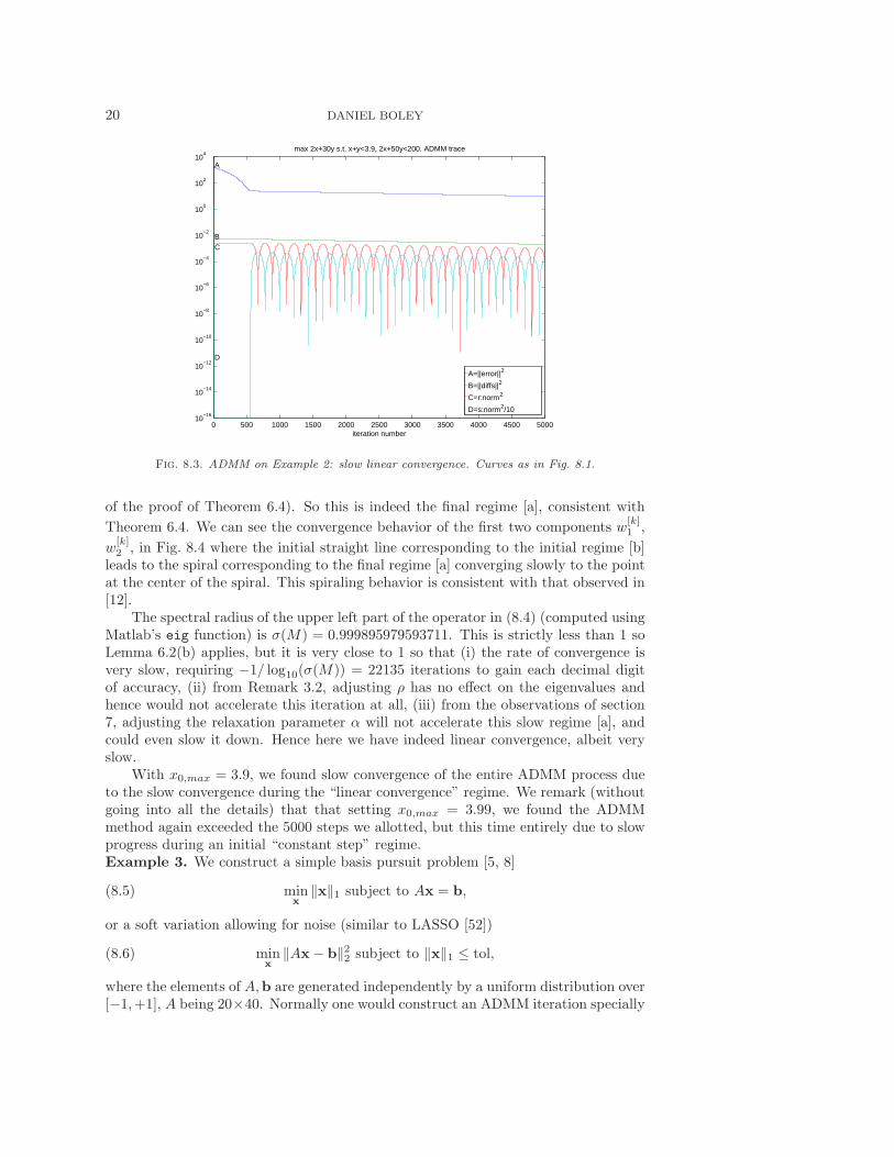
Fig. 8.3. ADMM on Example 2: slow linear convergence. Curves as in Fig. 8.1.
of the proof of Theorem 6.4). So this is indeed the final regime [a], consistent with
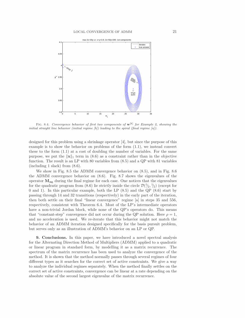
Theorem 6.4. We can see the convergence behavior of the first two components w[k]1 ,
w[k]2 , in Fig. 8.4 where the initial straight line corresponding to the initial regime [b]
leads to the spiral corresponding to the final regime [a] converging slowly to the pointat the center of the spiral. This spiraling behavior is consistent with that observed in[12].
The spectral radius of the upper left part of the operator in (8.4) (computed usingMatlab’s eig function) is σ(M) = 0.999895979593711. This is strictly less than 1 soLemma 6.2(b) applies, but it is very close to 1 so that (i) the rate of convergence isvery slow, requiring −1/ log10(σ(M)) = 22135 iterations to gain each decimal digitof accuracy, (ii) from Remark 3.2, adjusting ρ has no effect on the eigenvalues andhence would not accelerate this iteration at all, (iii) from the observations of section7, adjusting the relaxation parameter α will not accelerate this slow regime [a], andcould even slow it down. Hence here we have indeed linear convergence, albeit veryslow.
With x0,max = 3.9, we found slow convergence of the entire ADMM process dueto the slow convergence during the “linear convergence” regime. We remark (withoutgoing into all the details) that that setting x0,max = 3.99, we found the ADMMmethod again exceeded the 5000 steps we allotted, but this time entirely due to slowprogress during an initial “constant step” regime.Example 3. We construct a simple basis pursuit problem [5, 8]
minx
‖x‖1 subject to Ax = b,(8.5)
or a soft variation allowing for noise (similar to LASSO [52])
minx
‖Ax− b‖22 subject to ‖x‖1 ≤ tol,(8.6)
where the elements of A,b are generated independently by a uniform distribution over[−1,+1], A being 20×40. Normally one would construct an ADMM iteration specially
LOCAL CONVERGENCE OF ADMM 21
0 5 10 15 20 25 30 353.8
3.85
3.9
3.95
4
4.05
4.1max 2x+30y s.t. x+y<3.9, 2x+50y<200. 1st components
w1
w2
iteratestrue answer
←step
1
step5000→
↑truesoln
Fig. 8.4. Convergence behavior of first two components of w[k] for Example 2, showing theinitial straight line behavior (initial regime [b]) leading to the spiral (final regime [a]).
designed for this problem using a shrinkage operator [4], but since the purpose of thisexample is to show the behavior on problems of the form (1.1), we instead convertthese to the form (1.1) at a cost of doubling the number of variables. For the samepurpose, we put the ‖x‖1 term in (8.6) as a constraint rather than in the objectivefunction. The result is an LP with 80 variables from (8.5) and a QP with 81 variables(including 1 slack) from (8.6).
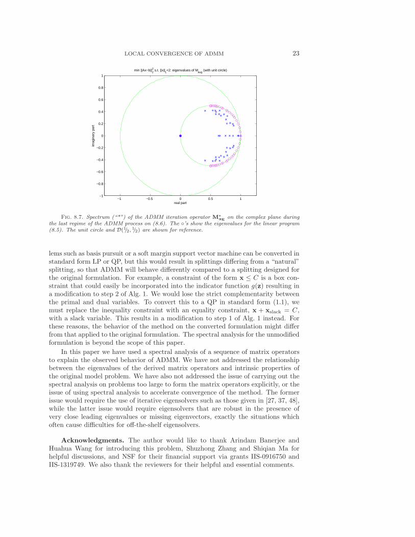
We show in Fig. 8.5 the ADMM convergence behavior on (8.5), and in Fig. 8.6the ADMM convergence behavior on (8.6). Fig. 8.7 shows the eigenvalues of theoperator Maug during the final regime for each case. One notices that the eigenvaluesfor the quadratic program from (8.6) lie strictly inside the circle D(1/2,
1/2) (except for0 and 1). In this particular example, both the LP (8.5) and the QP (8.6) start bypassing through 14 and 32 transitions (respectively) in the early part of the iteration,then both settle on their final “linear convergence” regime [a] in steps 35 and 556,respectively, consistent with Theorem 6.4. Most of the LP’s intermediate operatorshave a non-trivial Jordan block, while none of the QP’s operators do. This meansthat “constant-step” convergence did not occur during the QP solution. Here ρ = 1,and no acceleration is used. We re-iterate that this behavior might not match thebehavior of an ADMM iteration designed specifically for the basis pursuit problem,but serves only as an illustration of ADMM’s behavior on an LP or QP.
9. Conclusions. In this paper, we have introduced a novel spectral analysisfor the Alternating Direction Method of Multipliers (ADMM) applied to a quadraticor linear program in standard form, by modelling it as a matrix recurrence. Thespectrum of the matrix recurrence has been used to analyze the convergence of themethod. It is shown that the method normally passes through several regimes of fourdifferent types as it searches for the correct set of active constraints. We give a wayto analyze the individual regimes separately. When the method finally settles on thecorrect set of active constraints, convergence can be linear at a rate depending on theabsolute value of the second largest eigenvalue of the matrix recurrence.

22 DANIEL BOLEY
0 500 1000 150010
−16
10−14
10−12
10−10
10−8
10−6
10−4
10−2
100
102
iteration number
20 x 40 basis pursuit: min ||x||1 s.t. Ax=b. ρ= α=
A
B
C
D
A=||error||2
B=||diffs||2
C=r:norm2
D=s:norm2/10
Fig. 8.5. ADMM applied to the LP of Example 3 (8.5) using α = ρ = 1. Curves as in Fig. 8.1.
0 20 40 60 80 100 120 14010
−14
10−12
10−10
10−8
10−6
10−4
10−2
100
102
iteration number
20 x 40 basis pursuit: min ||Ax−b||2 s.t. ||x||
1<2; ρ= α=
A
B
C
D
A=||error||2
B=||diffs||2
C=r:norm2
D=s:norm2/10
Fig. 8.6. Unaccelerated ADMM applied to the QP of Example 3 (8.6) using α = ρ = 1. CurveA,B,C,D are as in Fig. 8.5.
The analysis in terms of regimes allows one to more effectively adjust accelerationmethods to match the current regime. For example, we have shown for LPs duringthe “linear convergence” regime, relaxation can be detrimental to the performance ofthe algorithm, while during “constant-step” regime it can be beneficial. Likewise withrespect to the proximity parameter ρ, while adjusting ρ can have a dramatic effect onthe rate of convergence in general, in LPs it has almost no effect on the asymptoticrate of convergence during the regime of linear convergence.
This paper is limited to LPs and QPs in standard form. In principle other prob-
LOCAL CONVERGENCE OF ADMM 23
−1 −0.5 0 0.5 1−1
−0.8
−0.6
−0.4
−0.2
0
0.2
0.4
0.6
0.8
1
min ||Ax−b||22 s.t. ||x||
1<2: eigenvalues of M
aug (with unit circle)
real part
imag
inar
y pa
rt
Fig. 8.7. Spectrum (“*”) of the ADMM iteration operator M∗aug on the complex plane during
the last regime of the ADMM process on (8.6). The ◦’s show the eigenvalues for the linear program(8.5). The unit circle and D(1/2, 1/2) are shown for reference.
lems such as basis pursuit or a soft margin support vector machine can be converted instandard form LP or QP, but this would result in splittings differing from a “natural”splitting, so that ADMM will behave differently compared to a splitting designed forthe original formulation. For example, a constraint of the form x ≤ C is a box con-straint that could easily be incorporated into the indicator function g(z) resulting ina modification to step 2 of Alg. 1. We would lose the strict complementarity betweenthe primal and dual variables. To convert this to a QP in standard form (1.1), wemust replace the inequality constraint with an equality constraint, x + xslack = C,with a slack variable. This results in a modification to step 1 of Alg. 1 instead. Forthese reasons, the behavior of the method on the converted formulation might differfrom that applied to the original formulation. The spectral analysis for the unmodifiedformulation is beyond the scope of this paper.
In this paper we have used a spectral analysis of a sequence of matrix operatorsto explain the observed behavior of ADMM. We have not addressed the relationshipbetween the eigenvalues of the derived matrix operators and intrinsic properties ofthe original model problem. We have also not addressed the issue of carrying out thespectral analysis on problems too large to form the matrix operators explicitly, or theissue of using spectral analysis to accelerate convergence of the method. The formerissue would require the use of iterative eigensolvers such as those given in [27, 37, 48],while the latter issue would require eigensolvers that are robust in the presence ofvery close leading eigenvalues or missing eigenvectors, exactly the situations whichoften cause difficulties for off-the-shelf eigensolvers.
Acknowledgments. The author would like to thank Arindam Banerjee andHuahua Wang for introducing this problem, Shuzhong Zhang and Shiqian Ma forhelpful discussions, and NSF for their financial support via grants IIS-0916750 andIIS-1319749. We also thank the reviewers for their helpful and essential comments.

24 DANIEL BOLEY
REFERENCES
[1] A. Beck and M. Teboulle, A fast iterative shrinkage-thresholding algorithm for linear inverseproblems, SIAM J. Imaging Sciences, 2 (2009), pp. 183–202.
[2] D. Bertsekas and J. Tsitsiklis, Parallel and Distributed Computation, Prentice Hall, 1989.[3] , Parallel and Distributed Computation: Numerical Methods, Athena Scientific, 1997.[4] S. Boyd, N. Parikh, E. Chu, B. Peleato, and J. Eckstein, Distributed optimization and sta-
tistical learning via the alternating direction method of multipliers, Foundations and Trendsin Machine Learning, 3 (2011), pp. 1–122. http://www.stanford.edu/~boyd/papers/admm/.
[5] A. M. Bruckstein, D. L. Donoho, and M. Elad, From sparse solutions of systems of equa-tions to sparse modeling of signals and images, SIAM Review, 51 (2009), pp. 34–81.
[6] T. F. Chan and R. Glowinski, Finite element approximation and iterative solution of a classof mildly nonlinear elliptic equations. technical report, Computer Science Department,Stanford University, 1978.
[7] C. H. Chen, B. S. He, and X. M. Yuan, Matrix completion via an alternating directionmethod, IMA J. Numer. Anal., 32 (2012), pp. 227–245.
[8] S. Chen and D. Donoho, Basis pursuit, in Signals, Systems and Computers, 1994. 1994Conference Record of the Twenty-Eighth Asilomar Conference on, vol. 1, 1994, pp. 41–44.
[9] E. Dall’Anese, J. A. Bazerque, and G. B. Giannakis, Group sparse LASSO for cognitivenetwork sensing robust to model uncertainties and outliers, Physical Communication, 5(2012), pp. 161–172.
[10] W. Deng and W. Yin, On the global and linear convergence of the generalized alternatingdirection method of multipliers. Rice Univ. CAAM Tech. Rep. TR12-14, 2012.
[11] J. Douglas and H. H. Rachford, On the numerical solution of the heat conduction problemin 2 and 3 space variables, Trans. Amer. Math. Soc., 82 (1956), pp. 421–439.
[12] J. Eckstein and D. P. Bertsekas, An alternating direction method for linear programming.MIT Lab. for Info. and Dec. Sys. report LIDS-P-1967, April 1990.
[13] J. Eckstein and D. P. Bertsekas, On the Douglas-Rachford splitting method and the proximalpoint algorithm for maximal monotone operators, Math. Program., 55 (1992), pp. 293–318.
[14] J. Eckstein and B. F. Svaiter, General projective splitting methods for sums of maximalmonotone operators, SIAM J. Control Optim., 48 (2009), pp. 787–811.
[15] T. Erseghe, D. Zennaro, E. Dall’Anese, and L. Vangelista, Fast consensus by the alter-nating direction multipliers method, IEEE Trans. Signal Proc., 59 (2011), pp. 5523–5537.
[16] E. Esser, Applications of Lagrangian-based alternating direction methods and connections tosplit Bregman. UCLA CAM Report 09-31, University of California, Los Angeles, 2009.
[17] M. Fukushima, Application of the alternating direction method of multipliers to separableconvex programming problems, Comput. Optim. Appl., 2 (1992), pp. 93–111.
[18] D. Gabay, Applications of the method of multipliers to variational inequalities,, in AugmentedLagrangian Methods: Applications to the Solution of Boundary-Value Problems, M. Fortinand R. Glowinski, eds., North-Holland: Amsterdam, 1983.
[19] D. Gabay and B. Mercier, A dual algorithm for the solution of non- linear variationalproblems via finite-element approximations, Comp. Math. Appl., 2 (1976), pp. 17–40.
[20] F. R. Gantmacher, The Theory of Matrices, Chelsea Publishing Company, New York, 1959.[21] R. Glowinski, T. Karkkainen, and K. Majava, On the convergence of operator-splitting
methods, in Numerical Methods for Scientific Computing, Variational Problems and Ap-plications, 2003. Barcelona.
[22] R. Glowinski and A. Marrocco, Sur l’approximation, par elements finis d’ordre un, et laresolution par penalisation-dualite, d’une classe de problemes de Dirichlet non lineaires,Revue Francaise d’Automatique, Informatique, et Recherche Operationelle, 9 (1975),pp. 41–76.
[23] R. Glowinski and P. Le Tallec, Augmented Lagrangian and Operator-Splitting Methods inNonlinear Mechanics, vol. 9, SIAM Studies in Applied and Numerical Mathematics, 1989.
[24] D. Goldfarb and S. Ma, Fast multiple-splitting algorithms for convex optimization, SIAM J.Optim., 22 (2012), pp. 533–556.
[25] D. Goldfarb, S. Ma, and K. Scheinberg, Fast alternating linearization methods for mini-mizing the sum of two convex functions, Math. Program. Ser. A, (2012), pp. 1–34.
[26] T. Goldstein, B. O’Donoghue, and S. Setzer, Fast alternating direction optimization meth-ods. CAM report 12-35, UCLA, 2012.
[27] G. H. Golub and C. F. Van Loan, Matrix Computations, Johns Hopkins Univ. Press, 4th ed.,2013.
[28] M. Grant and S. Boyd, CVX: Matlab software for disciplined convex programming, version1.21. http://cvxr.com/cvx, Apr. 2011.

LOCAL CONVERGENCE OF ADMM 25
[29] B. S. He and X. M. Yuan, On non-ergodic convergence rate of Douglas-Rachford alternat-ing direction method of multipliers. http://www.optimization-online.org/DB HTML/2012/
01/3318.html, 2012.[30] B. S. He and X. M. Yuan, On the O(1/n) convergence rate of the Douglas-Rachford alter-
nating direction method, SIAM J. Numer. Anal., 50 (2012), pp. 700–709.[31] B. S. He, L. Z. Liao, D. R. Han, and H. Yang, A new inexact alternating directions method
for monontone variational inequalities, Math. Program. Ser. A, 92 (2002), pp. 103–118.[32] B. S. He, M. H. Xu, and X. M. Yuan, Solving large-scale least squares semidefinite program-
ming by alternating direction methods, SIAM J. Matrix Anal. Appl., 32 (2011), pp. 136–152.[33] M. Hong and Z. Q. Luo, On the linear convergence of the alternating direction method of
multipliers. Arxiv preprint arXiv:1208.3922, 2012.[34] R. A. Horn and C. R. Johnson, Matrix Analysis, Cambridge University Press, Cambridge,
1985.[35] A. S. Householder, The Theory of Matrices in Numerical Analysis, Dover Publishing, New
York, 1964. Originally published by Ginn Blaisdell.[36] S. Kontogiorgis and R. R. Meyer, A variable-penalty alternating directions method for
convex optimization, Math. Program., 83 (1998), pp. 29–53.[37] R. B. Lehoucq, D. C. Sorensen, and C. Yang, ARPACK Users’ Guide: Solution of Large
Scale Eigenvalue Problems with Implicitly Restarted Arnoldi Methods, SIAM, 1998.[38] P. L. Lions and B. Mercier, Splitting algorithms for the sum of two nonlinear operators,
SIAM J. Numer. Anal., 16 (1979), pp. 964–979.[39] S. Ma and S. Zhang, An extragradient-based alternating direction method for convex mini-
mization. arXiv:1301.6308v1 [math.OC], 2013.[40] J. F. C. Mota, J. M. F. Xavier, P. M. Q. Aguiar, and M. Puschel, D-
ADMM: A communication-efficient distributed algorithm for separable optimization.arXiv:1202.2805v1 [math.OC], 2012.
[41] J. F. C. Mota, J. M. F. Xavier, P. M. Q. Aguiar, and M. Puschel, Distributed basispursuit, Signal Processing, IEEE Transactions on, 60 (2012), pp. 1942 –1956.
[42] Y. E. Nesterov, A method for unconstrained convex minimization problem with the rate ofconvergence o(1/k 2 ), Dokl. Akad. Nauk SSSR, 269 (1983), pp. 543–547.
[43] , Introductory Lectures on Convex Optimization, A Basic Course, vol. 87 of Appl. Op-tim., Kluwer Academic Publishers, Boston, 2004.
[44] , Smooth minimization for non-smooth functions, Math. Program. Ser. A, 103 (2005),pp. 127–152.
[45] , Gradient methods for minimizing composite objective function. CORE Discussion Paper2007/76, 2007. http://www.optimizationonline.org/DBFILE/2007/09/1784.pdf.
[46] M. K. Ng, P. Weiss, and X. M. Yuan, Solving constrained total-variation image restorationproblems via alternating direction methods, SIAM J. Sci. Comput., 32 (2010), pp. 2710–2736.
[47] J. M. Ortega, Numerical Analysis: A Second Course, Academic Press, New York, 1972.(republished by SIAM, 1990).
[48] Y. Saad, Numerical Methods for Large Eigenvalue Problems, SIAM, 2nd ed., 2011.[49] J. E. Spingarn, Partial inverse of a monotone operator, Appl. Math. Optim., 10 (1983),
pp. 247–265.[50] J. Sun and S. Zhang, A modified alternating direction method for convex quadratically con-
strained quadratic semidefinite programs, Euro. J. Oper. Res., 207 (2010), pp. 1210–1220.[51] M. Tao and X. M. Yuan, Recovering low-rank and sparse components of matrices from in-
complete and noisy observations, SIAM J. Optim., 21 (2011), pp. 57–81.[52] R. Tibshirani, Regression shrinkage and selection via the LASSO, Journal of the Royal Sta-
tistical Society. Series B (Methodological), 58 (1996), pp. 267–288.[53] R. Tibshirani, M. Saunders, S. Rosset, J. Zhu, and K. Knight, Sparsity and smoothness
via the fused LASSO, J. Royal Statist. Soc., 67 (2005), pp. 91–108.[54] P. Tseng, A modified forward-backward splitting method for maximal monotone mappings,
SIAM J. Control Optim., 38 (2000), pp. 431–446.[55] H. Wang and A. Banerjee, Online alternating direction method, in Proc. 29th Intl. Conf.
Machine Learning, 2012.[56] J. Yang and Y. Zhang, Alternating direction algorithms for L1–problems in compressive
sensing, SIAM J. Sci. Comput., 33 (2011), pp. 250–278.[57] C. H. Ye and X. M. Yuan, A descent method for structured monotone variational inequalities,
Optim. Methods Softw., 22 (2007), pp. 329–338.[58] K. Zhuang, G. N. Vemuri, and R. Mahadevan, Economics of membrane occupancy and
respiro-fermentation, Mol Syst Biol, 7 (2011).