UNIVERSITÀ DEGLI STUDI DI GENOVA

FACOLTÀ DI INGEGNERIA

Tesi di Laurea Specialisticain

INGEGNERIA MECCANICA

Local Stability Analysis of a

Coaxial Jet at low

Reynolds Number

Candidato:

Giacomo Gallino

Relatore:

Chiar.mo Prof.Alessandro Bottaro

Relatore:

Prof.François Gallaire

Anno accademico 2011/2012

Riassunto

La formazione di gocce in getti a bassi numeri di Reynolds è unfenomeno di grande interesse dal punto di vista ingegneristico, es-sendo molte le sue possibili applicazioni in diversi processi industriali.Solo per nominarne alcune: stampanti a getto d'inchiostro, processi diemulsicazione e estrusione di polimeri. Motivati da queste possibiliapplicazioni, abbiamo studiato la stabilità di getti coassiali in micro-canali. La congurazione sica osservata è una variante del classicoproblema di Rayleigh-Plateau, dove però imponiamo connamentodel getto. Da studi precedenti è stata osservata sperimentalmentela transizione tra situazioni dove il usso forma un getto (regimedi jetting) o dove forma delle gocce (regime di dripping). Il veri-carsi di questi due regimi è stato giusticato dal tipo di instabilitàpresente nel usso che può essere convettiva o assoluta. Eseguendoanalisi di stabilità locale per diverse coordinate assiali del usso, ab-biamo studiato il usso nella regione in cui si sviluppa e abbiamo pro-posto un'interpretazione dei meccanismi che regolano la transizionetra regime di jetting e regime di dripping.

i

Abstract

Droplets formation in jets at low Reynolds number is a phenomenonof great engineering interest because of its applicability in industrialprocesses. Just to name a few: ink-jet printing, emulsication processand polymer extrusion. Motivated by these possible applications, westudy the stability of coaxial biphasic jets in micro-channels. Thephysical conguration observed is a variant of the classical Rayleigh-Plateau problem, where we impose wall connement. In previousstudies it has been observed experimentally the transition betweensituations where the ow takes the forms of a jet (jetting regime)or where it forms droplets (dripping regime). These two regimes areexplained with the ow being convectively unstable or absolutely un-stable. Performing local stability analysis for various axial coordinateof the ow, we analyze the developing region and we propose an inter-pretation of the mechanisms that rule the transition between jettingand dripping regime.

iii

Acknowledgments

I would like to express my gratitude to all the people who have con-tributed to the realization of this project. Especially I want to thankAlessandro Bottaro and François Gallaire, they have supervised mywork and really helped me in this rst experience in the researchworld. My gratitude is also for the members of the lab (LFMI-EPFL)in which I've worked in these months spent in Switzerland: LauraAugello for her patience and availability; Mathias Nagel for his com-petence about the boundary element method; Francesco Viola andMarc-Antoine Habisreutinger for their knowledge and for the won-derful week-ends spent skiing in the Swiss Alps; Edouard Boujo whotaught me not only about FreeFem but also about climbing; Cristo-bal Arratia, Pierre-Thomas Brun, Vladislav Lugo and Yoan Mar-chand for their friendship that made me feel like at home duringthese months.

v

Preface

The work presented in this project is the result of a collaboration be-tween the Laboratory of Fluid Mechanics and Instabilities (LFMI),EPFL, Lausanne (Switzerland), and the Department of Civil, Chemi-cal and Environmental Engineering, University of Genova. The workhas been carried out under the supervision of Alessandro Bottaro(UNIGE) and François Gallaire, head director of the LFMI-EPFL.The whole active has been realized, between September 2012 andFebruary 2013 at the EPFL, as part of a wider project focused onthe stability analysis of ows at low Reynolds number; this is donein order to be able to predict droplets formation in micro-channels.

In the rst stage of the project I have written a MATLAB code,using the boundary element method, to simulate numerically thephysical phenomenon. In the second stage I have adapted an in-house MATLAB code (from LFMI) to my problem. These two toolsmake possible to perform stability analysis on the ow studied. Thenumerical tool that I have developed in the frame of the project willbe used to carry on studies on the stability of ows characterizedfrom low Reynolds number and axisymmetric congurations.

vii

Contents

Introduction 1

1 Base ow calculations 51.1 The base . . . . . . . . . . . . . . . . . . . . . . . . . 51.2 Mathematical formulation of the problem . . . . . . . 71.3 Stokes as boundary integral equation . . . . . . . . . 91.4 Numerical method . . . . . . . . . . . . . . . . . . . 121.5 Results from the base ow calculations . . . . . . . . 21

2 Local linear stability analysis 232.1 How does it work . . . . . . . . . . . . . . . . . . . . 232.2 Mathematical formulation of the problem . . . . . . . 252.3 Numerical method . . . . . . . . . . . . . . . . . . . 292.4 How to look at the results . . . . . . . . . . . . . . . 34

3 Results 393.1 Axial dependency of the results . . . . . . . . . . . . 393.2 Comparison with previous studies . . . . . . . . . . . 41

Conclusions and future developments 493.3 Conclusions . . . . . . . . . . . . . . . . . . . . . . . 493.4 Future developments . . . . . . . . . . . . . . . . . . 51

Bibliography 53

ix

Introduction

Stability of jets is of great engineering interest since the work ofRayleigh [1] and Plateau [2] about jets instability; in fact it is verycommon to nd this kind of phenomena in many industrial applica-tions from energy generation to chemical processes. The jets analyzedin this project model those found in applications, like ink-jet prin-ters (gure 1). Ink-printers are very interesting to study because thesame technology could also be used to manufacture high technologyproducts, for example polymer extrusion of use in the microchip in-dustry (gure 2). Other applications vary from food to biomedicalindustry, for example in the second one it could be important to knowif a drug injected in vein forms droplets before or after it touches theorgan to which it is destined.

The jets present in the applications described above belong to aparticular class: coaxial conned jets at low Reynolds number. Theconguration of the system we will study is composed of a micro-channel (the size of the radius of the channel is about 10−4m) wheretwo immiscible uids touch each other (cf. gure 2.2); the two u-ids can not mix because of surface tension. From experimental andanalytical studies this conguration has always yielded an instabilitythat leads to droplets formation, as we can see in gure 4. Sometimesthe droplet is formed just outside the inlet (dripping) and sometimeswe can identify a jet after which the droplet is formed (jetting). In [5]the stability of the fully developed ow (for which an analytical solu-tion exists under lubrication theory simplication) has been studied;the ow is always locally unstable, the criterion to predict dripping

1

Figure 1: Ink-jets, experimental study by Steve Hoath in [3].

Figure 2: Polymer extrusion presented in [4], the ow of hexadecanepush the polymer at the tip of the nozzle that detaching forms thedroplets.

2

Figure 3: Flow conguration, experimental study presented in [5].

Figure 4: Two dierent regimes of droplets formation, jetting anddripping, experimental study presented in [5].

3

or jetting regime is to look if the instability is absolute or convective.If it is absolute the instability is strong enough for the disturbanceto move upstream and the dripping regime is thus formed; otherwisethe instability is washed away from the ow and the jetting regime isreached. In [5] a qualitatively good transition region between drip-ping and jetting regime is found, although in some cases the dierencebetween the experimental results and the analytical solutions seemsquite signicant.

In this project the main idea is to perform local stability analy-sis in the developing region, where we believe important mechanismsregarding the droplets formation are localized. In this way, not ap-plying lubrication theory, we hope to have a deeper understanding ofthe phenomenon and to nd better agreement with the experimentalresults.

What is done, more in detail, is to nd a stable congurationof the system; since this is not physically possible, we will force thesystem to be stable. This stable conguration is found numericallywith a code written in MATLAB in the frame of this work, usingthe boundary elements method. How this is done will be explainedin chapter 1. Once the stable conguration is reached we performlocal stability analysis in the region close to the inlet. In practicewe add small perturbations at the stable solution and look if theconguration remains stable or not. The method to do this will beexplained in chapter 2. From the results in the developing regionwe should capture eects which are not taken into account whenlooking only at the developed region. For example, we could ndthat a ow that has a convective mode in the developed region isactually characterized from an absolute instability in the developingregion, this eventually leading to a dripping regime. On the otherhand a convective mode in the developing region could wash away anabsolute mode coming from the developed region, yielding the jettingregime.

4

Chapter 1

Base ow calculations

1.1 The base

To perform the stability analysis we rst need a stationary congu-ration of the system, the base ow is in fact a so called xed point,a base conguration that does not change if not perturbed. In ourcase we have a coaxial jet and we expect droplets formation when theinterface between the uids touches the axis. Droplets formation isthought to be caused from the surface tension between the two uidsthat drives the instability (ref. [1] and [2]).

In order to nd a solution without droplets formation we neglectthe terms responsible of the instability, this will be discussed more indetail in the next section. In gure 1.1 we can see a base ow obtainednumerically with the boundary elements method code developed inthis project, from this is possible to perform a local stability analysisas it will be described in chapter 2.

5

Figure 1.1: Base ow computed with boundary element method.

Figure 1.2: Observed domain.

6

1.2 Mathematical formulation of the pro-

blem

The phenomenon we want to observe allows us to do the followingsimplifying hypothesis

• Reynolds number tends to 0, this means that the inertial forcesare negligible compared to the viscous forces

• Stationary ow

• Axisymmetric ow

• Gravity terms negligible

Considering the hypothesis, the governing equations of the problemare the stationary Stokes and continuity equations for incompressi-ble ows for each uid (domain 1 and 2, cf. gure 1.2), neglectingexternal forces:

∇Pi + µi∇2Ui = 0,

∇ ·Ui = 0, i = 1, 2

with the following boundary conditions: no slip at the wall and sym-metry at the axis

Uz(R2) = 0, Ur(R2) = 0,∂Uz

∂r= 0, Ur = 0,

∂P

∂r= 0.

The inner and outer domains are then coupled with the followinginterface conditions:continuity of tangential stress

tT (σ2 − σ1) n = 0,

where t and n are the tangential and normal unit vectors at the

7

Figure 1.3: Normal and tangential unit vector to the interface.

interface (gure 1.3) and σ is the Newtonian stress tensor

σ =

−Pi + 2µi∂Uzi

∂zµi

(∂Uzi

∂r+

∂Uri

∂z

)µi

(∂Uzi

∂r+

∂Uri

∂z

)−Pi + 2µi

∂Uri

∂r

i = 1, 2.

Discontinuity of normal stress due to surface tension

nT (σ2 − σ1)n = γ1

R‖.

Note that we use only the curvature given by the inection of theinterface in the meridional plane (the plane containing the axis), thisis because we want to nd a stable solution of the system (base ow)and the azimuthal component 1/R⊥ causes the instability of the ow.

What we are doing is to force the system to be stable, we will add1/R⊥ later, together with the perturbations.The continuity of the velocities across the interface reads:

Ur1(R0) = Ur2(R0), Uz1(R0) = Uz2(R0),

and the impermeability of the interface is

Ur − Uz∂R0

∂z= 0,

R0 being the position of the interface.

8

Figure 1.4: Example of the computation of the velocity in (x0, y0)with boundary integral equations.

1.3 Stokes as boundary integral equation

To treat interface problems like the one we want to analyze it is veryconvenient to reformulate the governing equations of the system asintegral equations

αu(x0) = −∮l

G(x,x0)f(x)dl + µ

∮l

u(x)T (x,x0)n(x)dl. (1.1)

In equation 1.1 we have the boundary integral formulation of theStokes equation given in [6] for a domain Ω closed from a boundaryl.

α =

0 if x0 /∈ Ω

4πµ if x0 ∈ l8πµ if x0 ∈ Ω− l

G and T are the Green's functions for an axisymmetic domain, froma physical point of view they propagate the information applied atthe boundaries, in terms of stresses f and velocities u, to the otherparts of the domain (n is the unit vector normal to the boundarypointing inside the domain).

9

Figure 1.5: The two dierent domains coupled with the interfaceconditions.

For example to compute the velocity in (x0, y0) in gure 1.4 wejust have to perform an integration along the boundary l using equa-tion 1.1 with α = 8πµ. This has many advantages, for example thereis no need to mesh the inner domain, on the other hand the nume-rical treatment of the integral equation can be problematic in somesituations. As stated before, the implementation of this kind of equa-tion for a problem with interface is quite straightforward, in fact wecan imagine to have two separate domains in which we want to solve

10

Stokes equations (gure 1.5)

αu(x0) =−∫l1

G(x,x0)f(x)dl

+ µ1

∫l1

u(x)T (x,x0)n(x)dl

−∫int

G(x,x0)f(x)dl

+ µ1

∫int

u(x)T (x,x0)n(x)dl,

(1.2)

βu(x0) =−∫l2

G(x,x0)f(x)dl

+ µ2

∫l2

u(x)T (x,x0)n(x)dl

−∫int

G(x,x0)f(x)dl

+ µ2

∫int

u(x)T (x,x0)n(x)dl.

(1.3)

For these two domains we have the integral equations, 1.2 and 1.3,respectively. Summing 1.2 and 1.3 and taking into account the con-tinuity of the velocities and the discontinuity of the normal stress atthe interface ∆f = f2 + f1 = γ(1/R‖), we obtain

(α + β)u(x0) =−∫l1+l2

G(x,x0)f(x)dl

+ µ1

∫l1

u(x)T (x,x0)n(x)dl

+ µ2

∫l2

u(x)T (x,x0)n(x)dl

−∫int

G(x,x0)∆f(x)dl

+ (µ2 − µ1)

∫int

u(x)T (x,x0)n(x)dl,

(1.4)

11

where

α + β =

0 if x0 /∈ Ω1 + Ω2

4πµ1 if x0 ∈ l14πµ2 if x0 ∈ l28πµ1 if x0 ∈ Ω1 − l18πµ2 if x0 ∈ Ω2 − l24π(µ1 + µ2) if x0 ∈ interface.

The signs in equation 1.4, in the part regarding the interface, comefrom having considered positive the normal to the interface pointinginside the domain 2 (gure 1.5). Once the governing equation isdetermined, we impose the boundary conditions in order to close theproblem. In every point of the domain we have four variables, stressesand velocities in the axial and radial direction, in every point of theboundary we impose two of them. Looking at gure 1.2 we impose

• no slip condition at wall

• uniform normal stress and zero radial velocity at the outlet

• bi-Poiseuille axial velocity and zero radial velocity at the inlet

there is no need to impose anything on the axis because the Green'sfunctions already take in account the axisymmetric character of theproblem.

1.4 Numerical method

In this section it is explained how the integral equation 1.4 is solvednumerically. In gure 1.6 we can see how we discretize the boundaries.The position of the interface in the gure 1.6 is a guess position fromwhich we start the calculation, what we do is to nd the velocities inthe interface nodes and move them with these velocities after havingxed a ∆t.

12

Figure 1.6: Discretization of the problem.

This process is carried out until the velocities in these nodes sati-sfy the interface condition of impermeability, velocity normal to theinterface equal to zero (very small in our discretized case). In gure1.7 we see an example of evolution of the interface after a few it-erations. This approach is very good from a physical point of view,because it uses a physical criterion to move the interface, on the otherhand we must be very careful because of its explicit nature.

In fact, if we take too high ∆t the information given from onenode is moved too far (moving the node itself with its velocity) andthis gives rise to numerical oscillations. The nodes distribution isdone with the aim to have a ner mesh where we have discontinuouschanges in viscosity (where the interface touches inlet and outlet) andwhere we have a change in the boundary condition imposed (cornerpoints). We also have a higher density of nodes at the interface closeto the inlet, where the interface will bend more and the computationof the curvature will need to be more accurate. In every node ingure 1.6 a six points Gauss integration of the Green's functions isperformed, assuming stresses and velocities constants (cf. gure 1.8).

13

Figure 1.7: Iterative process to nd the interface position.

Figure 1.8: Six points Gauss integration for every node.

14

−1 −0.8 −0.6 −0.4 −0.2 0 0.2 0.4 0.6 0.8 1−5

−4

−3

−2

−1

0

1

2

3

4

5

x−x0

f

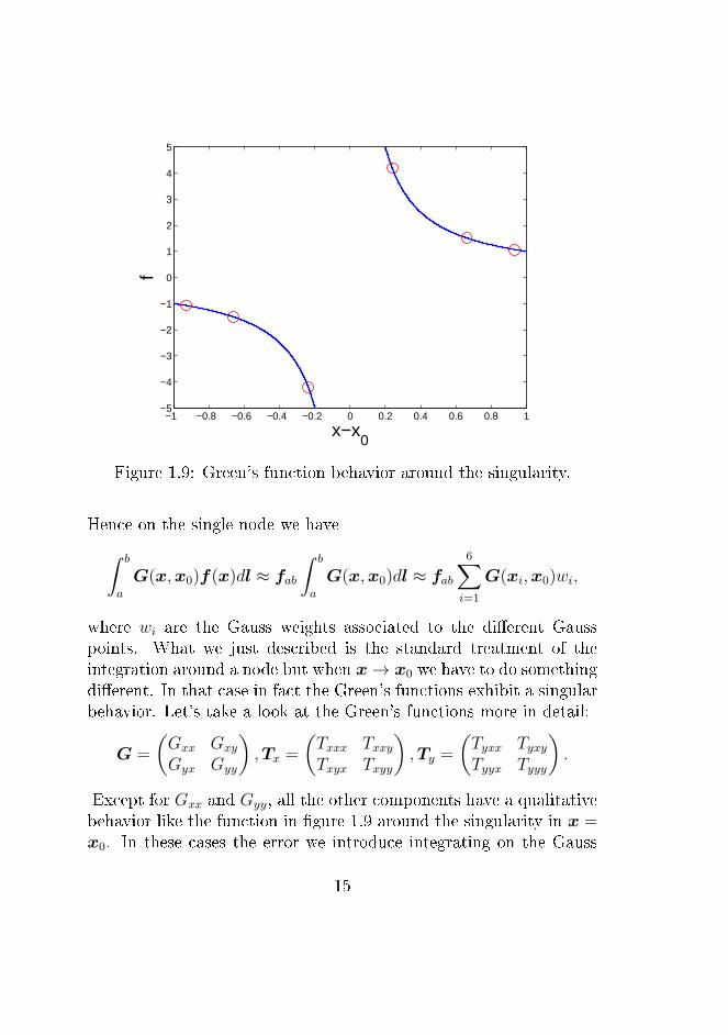
Figure 1.9: Green's function behavior around the singularity.

Hence on the single node we have∫ b

a

G(x,x0)f(x)dl ≈ fab∫ b

a

G(x,x0)dl ≈ fab6∑

i=1

G(xi,x0)wi,

where wi are the Gauss weights associated to the dierent Gausspoints. What we just described is the standard treatment of theintegration around a node but when x→ x0 we have to do somethingdierent. In that case in fact the Green's functions exhibit a singularbehavior. Let's take a look at the Green's functions more in detail:

G =

(Gxx Gxy

Gyx Gyy

),Tx =

(Txxx TxxyTxyx Txyy

),Ty =

(Tyxx TyxyTyyx Tyyy

).

Except for Gxx and Gyy, all the other components have a qualitativebehavior like the function in gure 1.9 around the singularity in x =x0. In these cases the error we introduce integrating on the Gauss

15

−1 −0.8 −0.6 −0.4 −0.2 0 0.2 0.4 0.6 0.8 10

5

10

15

20

25

x−x0

f

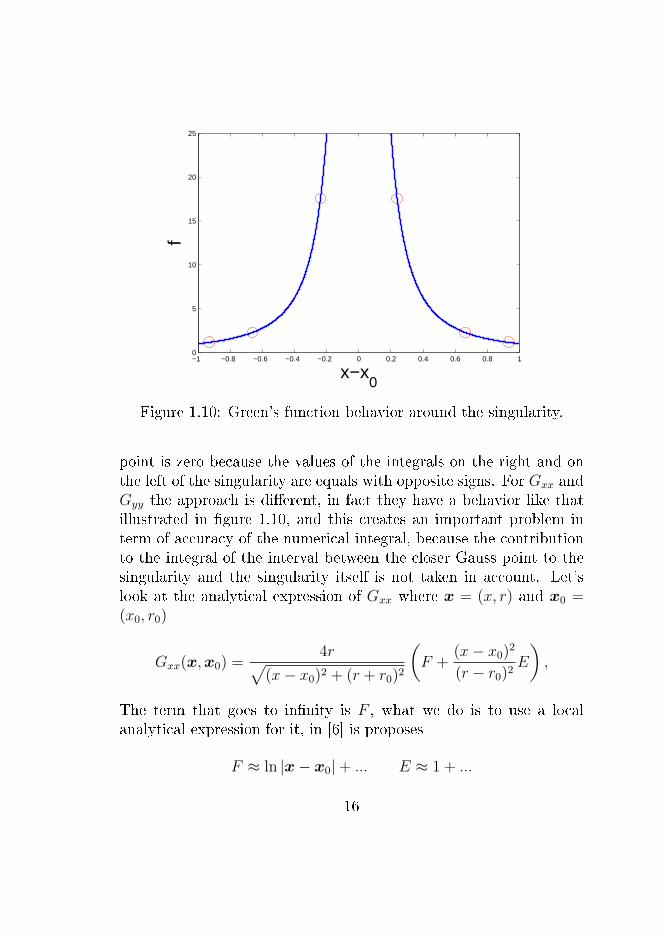
Figure 1.10: Green's function behavior around the singularity.

point is zero because the values of the integrals on the right and onthe left of the singularity are equals with opposite signs. For Gxx andGyy the approach is dierent, in fact they have a behavior like thatillustrated in gure 1.10, and this creates an important problem interm of accuracy of the numerical integral, because the contributionto the integral of the interval between the closer Gauss point to thesingularity and the singularity itself is not taken in account. Let'slook at the analytical expression of Gxx where x = (x, r) and x0 =(x0, r0)

Gxx(x,x0) =4r√

(x− x0)2 + (r + r0)2

(F +

(x− x0)2

(r − r0)2E

),

The term that goes to innity is F , what we do is to use a localanalytical expression for it, in [6] is proposes

F ≈ ln |x− x0|+ ... E ≈ 1 + ...

16

Taking the rst order expansion we obtain the local approximation

Gxx(x,x0) ≈ −2 ln |x− x0|+ 1, (1.5)

since 1.5 is analytically integrable, we can write∫ b

a

Gxx(x,x0)dl =

∫ b

a

(Gxx(x,x0) + 2 ln |x− x0|+ 1)dl+∫ b

a

(−2 ln |x− x0|+ 1)dl =∫ b

a

(Gxx(x,x0) + 2 ln |x− x0|+ 1)dl

+[− 2|x− x0| ln |x− x0|+ 3|x− x0|

]ba.

In this way we subtract the diverging part from the numerical integraland add it in an analytical form, keeping a good accuracy. Nowthat we have the integrals of the Green's functions for every nodes,we perform a numerical integral of the entire boundary l using therectangle method. If we have N nodes we obtain∮

l

G(x,x0)f(x)dl ≈N∑

n=1

fn

( 6∑i=1

G(xi,x0)wi

)n

.

This leads to a linear problem (2N unknowns in 2N equations) thatonce solved provides the velocities and the stresses on the boundariesand on the interface. These results are used as boundary conditionsto run a FreeFem [7] simulation using the nite elements method.We have chosen this approach because it would have taken too long(in the frame of this project) to have access to all the quantitieswe need to perform local stability analysis (stress tensor gradient)with the boundary elements method. On the other hand with theboundary elements method it is much easier to nd the interfaceposition, in gure 1.11 we can see a convergence study on the erroron the interface position in the fully developed region computed with

17

0 50 100 150 200 250 3000

5

10

15

20

25

30

35

nodes

erro

r %

Figure 1.11: Convergence study.

Figure 1.12: FreeFem mesh for domain 1 and 2.

18

Figure 1.13: Zoom of FreeFem mesh close to the inlet for domain 1and 2.

the boundary elements method, compared to the analytical solution.

FreeFem computations have been carried on by Edouard Boujo aformer Phd student at LFMI-EPFL; in these computations domain 1and 2 are computed separately like two dierent ows, in gure 1.12we can see the mesh in FreeFem based on the domain congurationfound with the boundary elements method, imposing the velocitiesas boundaries conditions, in gure 1.13 we may notice how the meshis ner close to inlet where our study is focused. In this way we ndthe pressure eld (gure 1.14), axial and radial velocities elds (gure1.15 and 1.16) in all the domain and we obtain all the quantities weneed to perform local stability analysis.

19

Figure 1.14: Pressure eld for domain 1 and 2.

Figure 1.15: Axial velocity eld for domain 1 and 2.

Figure 1.16: Radial velocity eld for domain 1 and 2.

20

Figure 1.17: Interface position for dierent ow rate ratio, λ = 0.6,Ka = 10.

Figure 1.18: Interface position for dierent viscosity ratio, Q = 0.5,Ka = 10.

1.5 Results from the base ow calculations

The problem is treated in function of three dimensionless numbers:the ow rate ratio, the viscosity ratio and the capillary number

Q =Q1

Q2

, λ =µ1

µ2

, Ka =∂zpR

22

γ.

Here are reported some ow conguration obtained with the bound-ary elements method code previously mentioned. As for the analyti-cal description we can notice how the interface position at the outletvaries when we change ow rate and viscosity ratios. Increasing theow rate and the viscosity ratio will move the interface toward thewall and vice versa, we can observe this behavior in gure 1.17 and1.18. The duration of the calculations is very dependent on the valueof the surface tension and on the velocity of the ow; these parame-ters are taken into account with the capillary number. The larger thepressure gradient is the more the velocity is high and the movement

21

of the interface is fast; then the calculation is fast. Opposite behavioris found when the surface tension is large, because this tends to makethe computation numerically unstable.

22

Chapter 2

Local linear stability analysis

2.1 How does it work

The aim of the stability analysis is to understand if a certain physicalconguration is stable when we apply small perturbations on it. Thecongurations to which we are going to add perturbations are calledxed points, this means that they wouldn't change their state if notperturbed. One common example of stable and unstable congura-tion is the ball at the bottom of the valley or on the top of a mountain(gure 2.1). In the rst case if we move the ball of an innitesimalspace (small perturbation), the ball will return in the initial positionafter an oscillation around the xed point. In the second case the

Figure 2.1: Stable and unstable congurations.

23

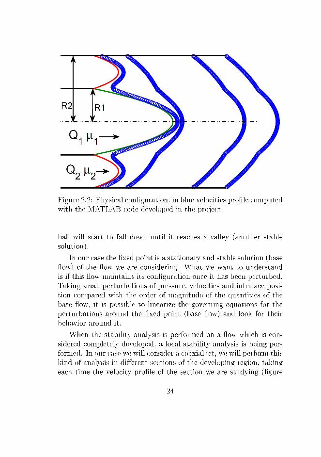
Figure 2.2: Physical conguration, in blue velocities prole computedwith the MATLAB code developed in the project.

ball will start to fall down until it reaches a valley (another stablesolution).

In our case the xed point is a stationary and stable solution (baseow) of the ow we are considering. What we want to understandis if this ow maintains its conguration once it has been perturbed.Taking small perturbations of pressure, velocities and interface posi-tion compared with the order of magnitude of the quantities of thebase ow, it is possible to linearize the governing equations for theperturbations around the xed point (base ow) and look for theirbehavior around it.

When the stability analysis is performed on a ow which is con-sidered completely developed, a local stability analysis is being per-formed. In our case we will consider a coaxial jet, we will perform thiskind of analysis in dierent sections of the developing region, takingeach time the velocity prole of the section we are studying (gure

24

2.2). We are thus doing a "local" analysis of a (mildly) non-parallelow.

2.2 Mathematical formulation of the pro-

blem

The assumptions of the local analysis lead to some important simpli-cations such as

Ur = 0,∂

∂z= 0,

from a physical point of view this means that the radial velocityis very small everywhere and the evolution of the ow in the axialdirection is slow compared to the wavelength of the perturbation.As it was stated in the previous section, small perturbations willbe summed to the quantities of the unperturbed ow, the base ow(capitol letters for the base ow quantities). That is

Uz

Ur

PR

=

Uz + εuz0 + εurP + εpR0 + εη

with ε 1.

Replacing the unperturbed quantities with the perturbed ones in thegoverning equations it is found

r : −∂P∂r− ε∂p

∂r+ µ

[1

r

∂

∂r

(rε∂ur∂r

)+ ε

∂2ur∂z2

− εurr2

]= 0,

z : −∂P∂z− ε∂p

∂z+ µ

[1

r

∂

∂r

(r∂Uz

∂r+ rε

∂uz∂r

)+∂2Uz

∂z2+ ε

∂2uz∂z2

]= 0,

ε∂ur∂r

+ εurr

+∂Uz

∂z+ ε

∂uz∂z

= 0.

Canceling the part verifying the governing equations for the base owand taking only the terms of order ε, we reach the linearized equation

25

for the perturbations

r : −∂p∂r

+ µ

[1

r

∂

∂r

(r∂ur∂r

)+∂2ur∂z2

− urr2

]= 0,

z : −∂p∂z

+ µ

[1

r

∂

∂r

(r∂uz∂r

)+∂2uz∂z2

]= 0,

∂ur∂r

+urr

+∂uz∂z

= 0.

In the same way we obtain the linearized boundary conditions

no slip at the wall: uz(R2) = 0, ur(R2) = 0,

symmetry on the axis: ur(0) = 0,∂uz∂r

∣∣∣0

= 0,∂p

∂r

∣∣∣0

= 0.

For the linearized interface conditions we have to consider the pertur-bation of the interface itself, than the conditions should be imposedat R0 + εη.

Let's see how these conditions should be applied, for example forthe continuity of axial velocity

Uz1(R0 + εη) + εuz1(R0 + εη) = Uz2(R0 + εη) + εuz2(R0 + εη). (2.1)

The problem is that from the computation of the base ow we don'tknow the position of the perturbed interface. We can however carryout a Taylor expansion around R0, the unperturbed interface point,to extract the quantities in the perturbed location (gure 2.3). Let'ssee an example for a generic function f

f(R0 + εη) = f(R0) +∂f

∂r

∣∣∣R0

εη.

In our case we obtain, for the continuity of the axial velocity

Uz1(R0 + εη) + εuz1(R0 + εη) =Uz1(R0) +∂Uz1

∂r

∣∣∣R0

εη

+ εuz1(R0) +∂uz1∂r

∣∣∣R0

ε2η,

26

Figure 2.3: "Flattening" hypothesis.

and similarly for the outer domain. Replacing in 2.1 and neglectingthe terms which satisfy the base ow interface conditions and theterms of order ε2 and smaller, we have:

uz1(R0) +∂Uz1

∂r

∣∣∣R0

η = uz2(R0) +∂Uz2

∂r

∣∣∣R0

η.

Following the same process we come to the other linearized interfaceconditions,the continuity of radial velocities

ur1(R0) +∂Ur1

∂r

∣∣∣R0

η = ur2(R0) +∂Ur2

∂r

∣∣∣R0

η,

that becomes ur1(R0) = ur2(R0) because Ur = 0 everywhere.The continuity of the tangential stress reads:

tT [(σ2 + εe2)− (σ1 + εe1)]n = 0,

where e is the Newtonian stress tensor for the perturbation and nand t are the perturbed normal and tangential unit vectors to theinterface (gure 2.3)

n =

(− ∂η

∂z, 1

)T

, t =

(1 ,

∂η

∂z

)T

,

27

we then come to write:(µ2∂2Uz2

∂r2−µ1

∂2Uz1

∂r2

)η+µ2

(∂uz2∂r

+∂ur2∂z

)−µ1

(∂uz1∂r

+∂ur1∂z

)= 0,

The balance of normal stress reads:

nT [(σ2 + εe2)− (σ1 + εe1)]n = γ

(1

R‖+

1

R⊥

),

that nally leads to(∂P1

∂r− ∂P2

∂r

)η + 2

(µ1∂Uz1

∂r− µ2

∂Uz2

∂r

)∂η

∂z+ p1 − p2

−2µ1∂uz1∂r

+ 2µ2∂uz2∂r

= −γ(η

R20

+∂2η

∂z2

).

Finally, the kinematic interface condition is:

∂η

∂t

∣∣∣∣R0

= ur1(R0)− U intz

∂η

∂z

∣∣∣∣R0

.

The unknowns of the problem are than substituted with the modalexpansion

ur = ur(r)ei(kz−ωt), uz = uz(r)e

i(kz−ωt),

p = p(r)ei(kz−ωt), η = ηei(kz−ωt).

Writing the unknowns in this way we split the radial evolution of theperturbations and the axial and temporal evolutions of the perturba-tions, the latter are included in the exponential term.

What we will do is to perturb the system in the space along theaxial direction, choosing a certain wavelength, trough k and see howit will react in time, looking at the ω we will nd. More in detailwe set a linear system containing the discretized Stokes equations fordomain 1 and 2 coupled with the interface condition equations. Thesystem has the following form:

Aϕ = 0,

28

where ϕ is the unknowns vector

ϕ =

(ur1 uz1 p1 ur2 uz2 p2 η

)T

,

and A is the matrix of the coecients of the linear system, which wecan write schematically as:

A =

[Domain 1] [0][0] [Domain 2]

[interface conditions]

This system has non trivial solution if and only if det(A) = 0; oncek is xed, the previous condition leads to an eigenvalue problem forω. We can then nd the complex parameter that determines thetemporal evolution of the perturbations

ω = ωr + iωi.

From the way in which the modal expansion is formulated, the com-plex part of ω will give the temporal evolution of the perturbation,i.e. its growth rate, the real part will give the temporal frequency ofthe perturbation.

2.3 Numerical method

In this project, the system shown in the previous section is solvednumerically with a in-house MATLAB code using a spectral method.The code, rst developed by Francesco Viola (former Phd studentat the LFMI-EPFL) to perform stability analysis on ows at highReynolds number, has been adapted for problems with interfacesat low Reynolds numbers. Replacing the unknowns of the problemwith their modal expansion we obtain, for a function f(r, z, t) =f(r)ei(kz−ωt)

∂f

∂z= f(r)ikei(kz−ωt),

∂f

∂t= −f(r)iωei(kz−ωt),

∂f

∂r=∂f

∂rei(kz−ωt),

29

this leads to a system of ODEs in r. The governing equation aremodied as follow:Stokes equation

r : µi

(1

r

durjdr

+d2urjdr2

− urik2 −urjr2

)− dpj

dr= 0,

z : µi

(1

r

duzjdr

+d2uzjdr2

− uzjk2)− ikpj = 0,

mass continuity

urjr

+durjdr

+ ikuzj = 0, j = 1, 2

impermeability of the interface

−iωη = ur1 − U intz kzη,

no slip condition at the wall

ur2(R2) = 0, uz2(R2) = 0,

symmetry condition at the axis:

ur1(0) = 0,∂uz1∂r

∣∣∣∣0

= 0,∂p1∂r

∣∣∣∣0

= 0,

continuity of the velocity at the interface

ur1(R0) = ur2(R0),

uz1(R0) +∂Uz1

∂r

∣∣∣R0

η = uz2(R0) +∂Uz2

∂r

∣∣∣R0

η,

continuity of tangential stress(µ2∂2Uz2

∂r2−µ1

∂2Uz1

∂r2

)η+µ2

(∂uz2∂r

+ikur2

)−µ1

(∂uz1∂r

+ikur1

)= 0,

30

−1 −0.8 −0.6 −0.4 −0.2 0 0.2 0.4 0.6 0.8 1−1

−0.8

−0.6

−0.4

−0.2

0

0.2

0.4

0.6

0.8

1

1234

Figure 2.4: Chebyshev polynomials of dierent degree.

balance of normal stress(∂P1

∂r− ∂P2

∂r

)η + 2

(µ1∂Uz1

∂r− µ2

∂Uz2

∂r

)ikη + p1 − p2

−2µ1∂uz1∂r

+ 2µ2∂uz2∂r

= −γ(

1

R20

− k2)η.

To perform the derivatives the domain is discretized in the radialdirection, thus every ODE become a system of linear equation. Toensure a good accuracy without high computational cost the codeemploys Chebyshev polynomials.

The nodes are determined from the roots of the Chebyshev poly-nomial, they are as much as the degree of the polynomial. In gure2.4 we can see Chebyshev polynomial of dierent degrees. Using thiskind of discretization, every node gives information to all the others.The computation of the derivate of a generic function f will be givenby the product between a full matrix times the vector containing the

31

Figure 2.5: Fitting the nodes in the physical domain.

values of f in the nodes.f ′1f ′2...f ′n

=

a11 a12 . . . a1na21 a22 . . . a2n...

.... . .

...an1 an2 . . . ann

f1f2...fn

The main advantage of this method is a really fast convergence (expo-nential if the function is smooth), this makes the method convenienteven if we have fully populated matrices. A drawback of the spec-tral collocation method is the fact that the distribution of the nodesis determined from the polynomials and it is not straightforward tomodify it.

In our code we have just changed the starting and ending point

32

of the polynomial (previously dened between −1 and 1) performinga linear mapping (gure 2.5) to t the physical domain we had toanalyze. Calling s the original independent variable of the Cheby-shev polynomial and R0 the position of the interface, the physicalcoordinate is for the domain 1 and 2 respectively

r1 =s+ 1

2R0, r2 = R0 + (R2 −R0)

s+ 1

2.

From this change of coordinate also the derivatives vary:rst derivatives

∂f

∂r1=∂f

∂s

∂s

∂r1=∂f

∂s

2

R0

,

∂f

∂r2=∂f

∂s

∂s

∂r2=∂f

∂s

2

R2 −R0

,

second derivatives, taking in account that s is a linear function of r

∂2f

∂r21=

∂f

∂s∂r1

∂s

∂r1+∂f

∂s

∂2s

∂r21=∂2f

∂s2

(∂s

∂r1

)2

=∂2f

∂s24

R20

,

∂2f

∂r22=∂2f

∂s24

(R2 −R0)2.

In gure 2.6 we can see a study on the convergence of the method thatconsiders the error on the maximum value of ωi compared with theanalytical solution in the completely developed region. This demon-strates that a resolution with 20 Chebyshev points (for each domain)is perfectly adequate for our purpose. The linear system is nallystructured in the following way

[Stokes r direction]1 0 0[Stokes z direction]1 0 0

[Continuity]1 0 00 [Stokes r direction]2 00 [Stokes z direction]2 00 [Continuity]2 0

impermeability of the interface

[ur1 ][uz1 ][p1][ur2 ][uz2 ][p2]η

= 0.

33

0 5 10 15 200

0.01

0.02

0.03

0.04

0.05

nodes

erro

r

Figure 2.6: Convergence study.

The rows in squared bracket are the ones that contain derivatives inthe radial direction, each of those is actually formed from as manylines as the number of nodes. The rst and last lines of these sectionscontain the boundary and interface conditions. In order to have anon trivial solution the determinant of the matrix is set equal to zeroleading to an eigenvalue problem to identify ω.

2.4 How to look at the results

To better treat the problem, we use the same adimensionalization asin [5]:

Q =Q1

Q2

, λ =µ1

µ2

, Ka =−∂zpR2

2

γ, k = kR1, ω =

16ωµ2R2

γ.

As function of Q, λ and Ka it is possible to uniquely determinethe shape of the interface and the velocity at the interface, we can

34

Figure 2.7: Interface position for Q = 0.7, λ = 0.5, Ka ≈ 1, R1 = 0.5.

thus study the problem in function of the independent dimensionlessvariable k and dependent variable ω.

From the numerical results in gure 2.8, we can observe that ωhas always the same shape also in dierent sections, that is also theshape of the analytical form found in [5] in the fully developed region:

ω = αk + iA

((k

b

)2

−(k

b

)4).

The dierence in our case is that A, b, and α, here constants onceQ, λ and Ka are chosen, depend on the axial coordinate at which weperform the analysis,

ω(z) = α(z)k + iA(z)

((k

b(z)

)2

−(

k

b(z)

)4).

Taking the base ow conguration in gure 2.7, we can see the nu-merical results for dierent axial coordinates in gure 2.8. Havingnoticed this similarity, we follow the same criterion used [5] to un-derstand if the regime is convective or absolutely unstable (cf. g2.9), and than if we expect to have jetting or dripping regime. Infact we can nd the back velocity v− and front velocity v+ of theperturbation imposing

v =ωi

ki,

∂ωi

∂kr= 0, v =

∂ωi

∂ki,

35

0 0.1 0.2 0.3 0.4 0.5 0.6 0.7 0.8 0.9 10

1

2

3

4

5

6

7

8

kad

ωr ad

z=0.1z=0.25z=0.5z=1z=2

0 0.1 0.2 0.3 0.4 0.5 0.6 0.7 0.8 0.9 1−0.1

0

0.1

0.2

0.3

0.4

0.5

0.6

kad

ωi ad

z=0.1z=0.25z=0.5z=1z=2

Figure 2.8: Real and imaginary part of ω for Q = 0.7, λ = 0.5,Ka ≈ 1, R1 = 0.5.

36

Figure 2.9: Wave packets propagating downstream and upstreamrespectively.

this criterion leads to

v± = α(z)± A(z)

(√7 + 5

12b(z)2−√

7 + 5

36b(z)4

)√24b(z)2√

7− 1.

We are interested in the back velocity v−, because if it is positivethe wave packet is washed away from the ow, if it's negative theperturbation can go upstream and propagate toward the inlet regionleading to dripping regime (gure 2.9). Let's see an example of v−in function of the axial coordinate (gure 2.10) We can observe thatclose to the inlet we have an absolute regime, this is physically co-herent because at the inlet the interface velocity is zero and then theperturbation can easily go upstream.

For this reason we will always expect an absolutely unstable regionclose to the inlet because the velocity at the interface we will not behigh enough to wash the perturbation away. This is why we putanother restriction for the instability to be absolute: we say that thelength of the absolute region LABS, has to be long enough to allowthe growth of the perturbation. Thus the minimum wavelength ofthe perturbation λmin must be shorter than the length of the absolute

37

0 0.2 0.4 0.6 0.8 1 1.2 1.4 1.6 1.8 2−1

−0.5

0

0.5

1

1.5

2

2.5

3

3.5

4

z

v −

Figure 2.10: Regime of the instability for Q = 0.7, λ = 0.5, Ka ≈ 1,R1 = 0.5.

regionLABS > λmin.

We should dene λmin with the frequency corresponding to the ab-solute mode of the perturbation, however we can dene in rst ap-proximation

λmin =2π

kcut off.

In the example in gure 2.10 we have LABS ≈ 0.125, much shorterthat λmin, and in this case, an absolute instability is not expected.

38

Chapter 3

Results

3.1 Axial dependency of the results

In this chapter we will present the dierences in the results of the localstability analysis computed in the region close to the inlet, comparedwith the results found for the fully developed ow. We also com-pare the results to the analytical solutions and experimental datapresented in [5]. Taking the ow conguration in gure 3.1, we canobserve the strong dependence of ω on the axial coordinate when wehave a considerable change of interface position between inlet andfully developed ow. In fact, in this case we have a position of theinterface around 0.5 (adimensional unit length) at the outlet and 0.1at the inlet. Looking at gure 3.2, we notice the dierent behavior of

Figure 3.1: Interface position for Q = 0.7, λ = 0.5, Ka = 1, R1 = 0.1.

39

0 0.5 1 1.50

2

4

6

8

10

12

14

kad

ωr ad

x=0.2x=0.25x=0.3x=0.36x=0.4x=0.6x=0.8x=1x=2x=3

0 0.5 1 1.5−3.5

−3

−2.5

−2

−1.5

−1

−0.5

0

0.5

1

1.5

kad

ωi ad

x=0.2x=0.25x=0.3x=0.36x=0.4x=0.6x=0.8x=1x=2x=3

Figure 3.2: Real and imaginary part of ω for Q = 0.7, λ = 0.5,Ka = 1, R1 = 0.1.

40

0 0.5 1 1.5 2 2.5 31

1.5

2

2.5

3

3.5

4

4.5

x

v −

Figure 3.3: Regime of the instability for ω for Q = 0.7, λ = 0.5,Ka = 1, R1 = 0.1.

both real and imaginary part of ω at dierent sections. This under-lines the fact that it is indeed important to analyze the developingregion because it could give quite dierent results from the regionwhere the ow is fully developed. In gure 3.3 we observe that theregime of the instability is convective everywhere in this case since thevelocity of the upstream front of the wave packet is always positive.

3.2 Comparison with previous studies

Here we analyze a case that in the analytic solution proposed in [5]is on the threshold between absolute and convective instability (theconguration is shown in gure 3.4). In gure 3.5 we can see the bluepoint, that identify the case we analyze, overlapped to the line that

41

Figure 3.4: Interface position for Q = 0.5636, λ = 0.2, Ka = 1,R1 = 0.2.

0 0.2 0.4 0.6 0.8 110

−6

10−5

10−4

10−3

10−2

10−1

100

101

interface position

Ka

case analyzedthreshold

absolute regime

convective regime

Figure 3.5: Absolute and convective regions in the (x,Ka) planefound analytically in [5].

42

0 0.5 1 1.50

5

10

15

20

25

kad

ωr ad

x=0.2x=0.25x=0.3x=0.36x=0.4x=0.6x=0.8x=1x=2x=3

Figure 3.6: Real part of ω for Q = 0.5636, λ = 0.2, Ka = 1, R1 = 0.2.

gives the threshold between absolute and convective region foundin [5]. This is a really interesting situation to observe because wecan understand if our model gives a more convectively or absolutelyunstable solution with respect to the analytical solution cited before.

In gure 3.6 and 3.7 the real and complex part of ω are shown,and from these the nature of the instability can be inferred (cf. g.3.8 where results at dierent sections z are reported). In gure 3.9we can see the eigenfunctions corresponding to the maximum valueof v− in the developing region and to the fully developed region. Tocompare the results shown in 3.8 with the analytical solution we haveto look at the fully developed ow, that corresponds to the v− valueson the right of the graph. Here we can notice a clearly convective be-havior, and this agrees well with the experimental results in [5], where

43

0 0.5 1 1.5−8

−6

−4

−2

0

2

4

kad

ωi ad

x=0.2x=0.25x=0.3x=0.36x=0.4x=0.6x=0.8x=1x=2x=3

Figure 3.7: Imaginary part of ω for Q = 0.5636, λ = 0.2, Ka = 1,R1 = 0.2.

0 0.5 1 1.5 2 2.5 31.5

2

2.5

3

3.5

4

4.5

5

5.5

z

v −

Figure 3.8: Regime of the instability for ω for Q = 0.5636, λ = 0.2,Ka = 1, R1 = 0.2.

44

0 0.2 0.4 0.6 0.8 10

0.2

0.4

0.6

0.8

1

ur1

ur2

uz1

uz2

p1p2

0 0.2 0.4 0.6 0.8 10

0.2

0.4

0.6

0.8

1

ur1

ur2

uz1

uz2

p1p2

Figure 3.9: Eigenfunctions for z = 0.3 and z = 3.5.

45

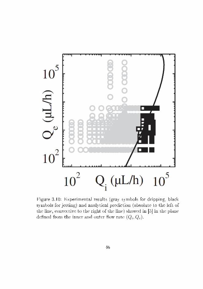
Figure 3.10: Experimental results (gray symbols for dripping, blacksymbols for jetting) and analytical prediction (absolute to the left ofthe line, convective to the right of the line) showed in [5] in the planedened from the inner and outer ow rate (Qi, Qe).

46

Figure 3.11: Droplets formation in an intermediate regime betweendripping and jetting, experimental study presented in [5].

the experimental data give jetting regime (convective), whereas theanalytical solution indicates an absolutely unstable behavior. In -gure 3.10 we can notice that the dierences between experimentaldata and analytical solutions are signicant, considering that a loga-rithmic scale is used.

It is also of great interest the peak for v− that we nd in thedeveloping region; since this value is higher then the value found forthe fully developed region, we could expect a positive v− even if itis negative in the fully developed region. This particular behavior ofv− (observed both in g. 3.3 and g. 3.8) could explain why in somecases the droplets form neither at the inlet nor in the fully developedregion, but in the middle (cf. g. 3.11). It is possible that thedisturbance moves upstream from the fully developed region towardthe inlet, and this movement would stop when v− changes sign.

47

Conclusions and future

developments

3.3 Conclusions

The tool developed in this project makes possible to perform localstability analysis on a coaxial jet for dierent axial coordinates, fromthe inlet to the fully developed region. What has been observedis the regime (absolute or convective instability) of dierent owsat dierent sections in order to determine whenever the system willgive rise to droplets formation at the inlet (dripping) or in the fullydeveloped region (jetting).

The study has the purpose to improve our understanding of theresults obtained in [5], for the transition between absolute and con-vective regime. To do that we have focused our attention on valuesof the parameters governing the problem, for which the ow is closeto threshold between absolute and convective regime. Doing thiswe have been able to have a good comparison between our model,the analytical solutions and the experimental results presented in [5].The results found are in good agreement with the experimental data;in addition they provide a basis for a better understanding of thephenomena going on in the developing region of the ow.

49

0 0.5 1 1.5 2 2.5 3−2.5

−2

−1.5

−1

−0.5

0

0.5

1

z

v −

Figure 3.12: Hypothesis on the behavior of the parameter v− in thecase of a mixed absolute and convective regime, v− determines theabsolute (when is negative) or convective (when is positive) regimeof the ow.

50

3.4 Future developments

The rst attempt to improve these results would be to nd a owthat exhibits a convective regime and absolute regime together, onein developing region and the other in the fully developing region (cf.g. 3.12). This case would be of great interest in justifying thetransition between dripping and jetting.

The following step would be to perform a global stability analy-sis, in order to take into account the variation of the system in theaxial direction. This is probably the best theoretical tool to analyzethis phenomenon and remains the main idea to follow in a possiblecontinuation of this project.

51

Bibliography

[1] Lord Rayleigh, On the Capillary Phenomena, Proceedings of theLondon Mathematical Society, Vol. XXIX, pp.71-97 (1879).

[2] Joseph Plateau, Statique Experimentale et Theorique des Liquidessoumis aux Seules Forces Moleculaires, Gauthier-Villars, Paris,(1873).

[3] Steve Hoats, Inkjet Printing - the Physics of Manipulating Liquid

Jets and Drops, Journal of Physics 105, 012001 (2008).

[4] Jeong Rim Hwang,Michael V. Sefton, Eect of capsule diame-

ter on the permeability to horseradish peroxidase of individual

HEMA-MMA microcapsules, Journal of Controlled Release, Vol-ume 49, Issues 23, Pages 217-227 (1997).

[5] Pierre Guillot, Annie Colin, Andrew S. Utada, Armand Ajdari,Stability of a Jet in Conned Pressure-Driven Biphasic Flows

at Low Reynolds Numbers, Physical Review Letters 99, 104502(2007).

[6] Constantine Pozrikidis, Boundary Integral and Singularity Meth-

ods for Linearized Viscous Flow, Cambridge University Press(1992).

[7] http://www.freefem.org/

53