localization using imu/gps sensors for mobility assistant ... · localization using imu/gps sensors...
TRANSCRIPT
Localization using IMU/GPS Sensors ForMobility Assistant for Visually Imparied
System (MAVI)
A thesis submitted in partial fulfillment of the requirement for the degreeof
Master of Technology
in
Integrated Electronics and Circuits
by
K. Hassen Basha2014EEN2790
Under the guidance of
Prof. M. Balakrishnan
Department of Electrical Engineering,Indian Institute of Technology Delhi.
June 2016.
Certificate
This is to certify that the project titled Localization using IMU/GPS
Sensors being submitted by K Hassen Basha, Entry No.2014EEN2790,
to the Department of Electrical Engineering, Indian Institute of
Technology Delhi, India, in partial fulfillment of requirements for the
award of the degree of Master of Technology in Integrated Electronics and
Circuits, is a bonafide record of research work carried out by him under my
guidance and supervision. The work presented in this thesis has not been
submitted elsewhere either in part or full, for the award of any other degree.
Prof. M.Balakrishnan
Department of Computer Science and Engineering
Indian Institute of Technology, Delhi
Abstract
The objective of location using GPS/IMU Sensors project is used to find
the accurate location of pedestrian. This location is used to store the lo-
cal sign board information into database. This information can be accessed
dynamically to find out the Sign board information. The localization using
GPS/IMU application can be efficiently implemented using Hardware/Software
co-design methodology.
The embedded applications can be better implemented using Xilinx Zynq All
Programmable System-on-Chip device as it has ARM processor core along
with the programmable FPGA fabric on the same chip. This approach facil-
itates the acceleration based implementations which can further optimized
for performance.
With the help of IMU, we can find out position increments. These incre-
ments can be aided with the GPS to calculate the current location. The
Kalman filter predicts and corrects the errors in the IMU and updates the
position to improve the accuracy.
The location using GPS/IMU integration was implemented on Zed Board.
The custom SDSoC platform was created to capture the GPS and IMU data
at various sampling rates. The fusion algorithm was implemented on proces-
sor of the Zed Board. The sensors were connected to PL of Zynq FPGA and
data captured using UART protocol.
The fusion algorithm was profiled using the SDSoC tool. The hotspots in
the algorithm were identified and realized in the hardware. The Kalman fil-
ter function was identified as a hotspot. This function is synthesized using
Vivado-HLS optimally to improve the overall performance of the system.

Acknowledgment
I take this opportunity to express my sincere regards to my supervisor Prof.
M. Balakrishnan, Department of Computer Science, for providing an oppor-
tunity to work under his supervision. I am grateful to him for providing
necessary suggestions and guidance during the course of this work. I learnt
how to approach a problem, explore possible solutions, analyze them criti-
cally and come up with an efficient solution. Without his support, this work
would not have been possible.
I would also like to thank Dr. Chetan Arora for his valuable insights and
assistance regarding subject of Computer Vision.
I also extent my thanks to Mr. Rajesh Kedia and Mrs. Radhika for having
useful discussions and providing us with ideas, Mr. Sharma (DHD) for pro-
viding me with all the lab equipments and support.
My heartfelt thanks to Munib Fazal and Yoosuf KK for making my thesis
journey fun filled and memorable.
I would like to thank Akshay Jain and Siva Krishna for their help and sug-
gestions. I am very grateful to my parents and well-wishers for their support.
K Hassen Basha
Contents
1 INTRODUCTION 1
1.1 Mobility Assistant for Visually Impaired (MAVI) . . . . . . . 1
1.2 Thesis Organization . . . . . . . . . . . . . . . . . . . . . . . . 3
2 Literature Review 4
3 IMU, GPS and Kalman Filtering 6
3.1 Inertial Measurement Unit . . . . . . . . . . . . . . . . . . . . 6
3.2 Reference Frames and Transformations . . . . . . . . . . . . . 6
3.2.1 The Inertial frame . . . . . . . . . . . . . . . . . . . . 7
3.2.2 The Earth Frame . . . . . . . . . . . . . . . . . . . . . 7
3.2.3 The Navigation Frame . . . . . . . . . . . . . . . . . . 8
3.2.4 The Body Frame . . . . . . . . . . . . . . . . . . . . . 10
3.3 Equations of Motion . . . . . . . . . . . . . . . . . . . . . . . 10
3.3.1 Errors in the IMU . . . . . . . . . . . . . . . . . . . . 15
3.4 Global Positioning System . . . . . . . . . . . . . . . . . . . . 15
3.4.1 Limitations and Errors in GPS . . . . . . . . . . . . . 17
3.5 Sensor Fusion Theory . . . . . . . . . . . . . . . . . . . . . . . 18
3.5.1 Kalman Filter . . . . . . . . . . . . . . . . . . . . . . . 19
3.5.2 Implementation of a Digital Kalman Filter . . . . . . . 22
3.5.3 GPS/IMU integration . . . . . . . . . . . . . . . . . . 23
4 Sensor Characterization 25
4.1 GPS . . . . . . . . . . . . . . . . . . . . . . . . . . . . . . . . 25
4.1.1 Key Features . . . . . . . . . . . . . . . . . . . . . . . 25
4.2 IMU . . . . . . . . . . . . . . . . . . . . . . . . . . . . . . . . 25
c© 2016, Indian Institute of Technology Delhi
CONTENTS 5
4.2.1 Accelerometer Bias . . . . . . . . . . . . . . . . . . . . 26
4.2.2 Gyroscope Bias . . . . . . . . . . . . . . . . . . . . . . 26
4.3 Calibration using Arduino . . . . . . . . . . . . . . . . . . . . 27
4.4 Configuration Registers of IMU . . . . . . . . . . . . . . . . . 27
4.4.1 Accelerometer . . . . . . . . . . . . . . . . . . . . . . . 27
4.4.2 Gyroscope . . . . . . . . . . . . . . . . . . . . . . . . . 27
4.4.3 Magnetometer . . . . . . . . . . . . . . . . . . . . . . . 29
5 Hardware Implementation 31
5.1 Overview . . . . . . . . . . . . . . . . . . . . . . . . . . . . . . 31
5.2 Architecture . . . . . . . . . . . . . . . . . . . . . . . . . . . . 32
5.2.1 Processing System . . . . . . . . . . . . . . . . . . . . 32
5.2.2 Programmable Logic . . . . . . . . . . . . . . . . . . . 33
5.2.3 Interconnect Features . . . . . . . . . . . . . . . . . . . 33
5.2.4 AXI Interconnect Types . . . . . . . . . . . . . . . . . 34
5.3 UART . . . . . . . . . . . . . . . . . . . . . . . . . . . . . . . 34
5.4 Co-ordinate Conversion . . . . . . . . . . . . . . . . . . . . . . 36
5.4.1 System Generator . . . . . . . . . . . . . . . . . . . . . 36
5.4.2 Fixed Point Implementation . . . . . . . . . . . . . . . 36
5.4.3 Single Point Implementation . . . . . . . . . . . . . . . 36
5.4.4 Double Precision Floating Point . . . . . . . . . . . . . 37
5.5 Data capture module for GPS . . . . . . . . . . . . . . . . . . 38
5.6 Complete Conversion for GPS . . . . . . . . . . . . . . . . . . 39
5.6.1 Debug using Chip scope Pro . . . . . . . . . . . . . . . 40
5.6.2 Vivado-SDK implementation . . . . . . . . . . . . . . . 41
5.7 Data Capture module for IMU . . . . . . . . . . . . . . . . . . 41
5.8 Complete IMU and GPS data Capture . . . . . . . . . . . . . 43
c© 2016, Indian Institute of Technology Delhi
CONTENTS 6
6 Custom SDSoC Platform Creation 44
6.1 Development Tools . . . . . . . . . . . . . . . . . . . . . . . . 44
6.1.1 Vivado IDE . . . . . . . . . . . . . . . . . . . . . . . . 44
6.1.2 Vivado HLS . . . . . . . . . . . . . . . . . . . . . . . . 44
6.1.3 Xilinx SDK . . . . . . . . . . . . . . . . . . . . . . . . 45
6.1.4 Xilinx SDSoC . . . . . . . . . . . . . . . . . . . . . . . 46
6.2 SDSoC Platform . . . . . . . . . . . . . . . . . . . . . . . . . 48
6.2.1 Steps to Generate SDSoc Hardware Platform Description 49
6.2.2 Steps to generate SDSoC Software Plaform Description 51
7 Software Implementation and Acceleration Using Vivado-
HLS 54
7.1 Functions implemented in SDK . . . . . . . . . . . . . . . . . 54
7.1.1 IEEE-74 Single Point to Hex Conversion . . . . . . . . 54
7.1.2 Hex to IEEE-754 Single Point Float Conversion . . . . 54
7.1.3 Fixed Point to Hex Conversion . . . . . . . . . . . . . 55
7.1.4 Hex to Fixed Point Conversion . . . . . . . . . . . . . 55
7.2 SDSoC implementation . . . . . . . . . . . . . . . . . . . . . 55
7.2.1 IMU Mechanization . . . . . . . . . . . . . . . . . . . . 55
7.2.2 Kalman Filter module . . . . . . . . . . . . . . . . . . 56
7.3 Accelerator Synthesis using Vivado HLS . . . . . . . . . . . . 56
7.3.1 Synthesize of Kalman Filter . . . . . . . . . . . . . . . 57
8 Performance and Power Measurements 58
8.1 Hardware setup for Power and Energy measurement . . . . . . 58
8.2 Sensor Power Measurement . . . . . . . . . . . . . . . . . . . 59
9 Conclusion and Future Work 63
9.1 Future Work . . . . . . . . . . . . . . . . . . . . . . . . . . . . 63
c© 2016, Indian Institute of Technology Delhi

Bibliography 64

List of Figures
1.1 Overview of MAVI System . . . . . . . . . . . . . . . . . . . 1
3.1 The inertial Frame [23] . . . . . . . . . . . . . . . . . . . . . 7
3.2 The Navigation Frame [24] . . . . . . . . . . . . . . . . . . . 9
3.3 Euler Angles . . . . . . . . . . . . . . . . . . . . . . . . . . . . 11
3.4 The Navigation Frame INS mechanization [24] . . . . . . . . 15
3.5 The Linear Kalman Filter Operation Cycle [21] . . . . . . . . 22
3.6 Loosely coupled GPS-INS integrated system . . . . . . . . . . 24
3.7 Tightly coupled GPS-INS integrated system . . . . . . . . . . 24
5.1 Zynq Features . . . . . . . . . . . . . . . . . . . . . . . . . . . 31
5.2 The Zynq Processing System [30] . . . . . . . . . . . . . . . . 32
5.3 The Interconnect Features [30] . . . . . . . . . . . . . . . . . . 34
5.4 UART Input/Ouput Ports . . . . . . . . . . . . . . . . . . . . 35
5.5 Single Precision Floating Point Representation . . . . . . . . . 37
5.6 Double Precision Floating Point Representation . . . . . . . . 37
5.7 Controller Module Input/ Output Ports . . . . . . . . . . . . 39
5.8 Error in X-Co-ordinate . . . . . . . . . . . . . . . . . . . . . . 42
5.9 Error in Y-Co-ordinate . . . . . . . . . . . . . . . . . . . . . . 42
5.10 Error in Z-Co-ordinate . . . . . . . . . . . . . . . . . . . . . . 42
6.1 Behavioural Synthesis using Vivado HLS [28] . . . . . . . . . . 45
6.2 SDSoC Design Flow [10] . . . . . . . . . . . . . . . . . . . . . 48
6.3 Directory Structure for a Typical SDSoC Platform [10] . . . . 49
8.1 Hardware Setup for Energy Measurement for ZedBoard . . . . 58
8.2 Power Measurement at Varies Sampling Rates of IMU Sensor 60
c© 2016, Indian Institute of Technology Delhi
8.3 Accuracy Measurement at Various Sampling Rates of IMU
Sensor . . . . . . . . . . . . . . . . . . . . . . . . . . . . . . . 61
8.4 Energy Measurement Vs Sampling Rates of IMU Sensor . . . 62
List of Tables
3.1 Sensor Errors in the IMU [20] . . . . . . . . . . . . . . . . . . 16
4.1 Variance of Accelerometer and Gyroscope . . . . . . . . . . . 26
4.2 Register 0x2C-BW RATE(Read/Write) . . . . . . . . . . . . . 27
4.3 Register 0x2C-BW RATE(Read/Write) . . . . . . . . . . . . . 28
4.4 Register 0x15 (Read/Write) . . . . . . . . . . . . . . . . . . . 28
4.5 Register 0x16 (Read/Write) . . . . . . . . . . . . . . . . . . . 28
4.6 Register 0x16-Bits(4-3) (FS SEL) . . . . . . . . . . . . . . . . 29
4.7 Register 0x16-Bits(2-0) (DLPF CFG) . . . . . . . . . . . . . . 29
4.8 Configuration of Register A . . . . . . . . . . . . . . . . . . . 29
4.9 Configuration of Register A Bit Designations . . . . . . . . . . 30
5.1 UART Resource Utilization . . . . . . . . . . . . . . . . . . . 35
5.2 Co-ordinate Conversion Resource Utilization . . . . . . . . . . 37
5.3 Controller Module Resource Utilization . . . . . . . . . . . . . 39
5.4 Complete Conversion for GPS Resource Utilization . . . . . . 40
5.5 Complete Conversion (Vivado) Resource Utilization . . . . . . 41
5.6 IMU module Resource Utilization . . . . . . . . . . . . . . . . 43
5.7 Complete IMU and GPS data Capture Resource Utilization . 43
7.1 Kalman Filter Performance . . . . . . . . . . . . . . . . . . . 57
7.2 Kalman Filter Resource Utilization . . . . . . . . . . . . . . . 57
8.1 Sensor Only Power Measurement . . . . . . . . . . . . . . . . 59
8.2 Processing Power Measurement . . . . . . . . . . . . . . . . . 60
8.3 Sampling Rate Power Measurement . . . . . . . . . . . . . . . 60
c© 2016, Indian Institute of Technology Delhi

LIST OF TABLES 11
8.4 Accuracy Measurement at Various Sampling Rates of IMU
Sensor . . . . . . . . . . . . . . . . . . . . . . . . . . . . . . . 61
8.5 Kalman Filter Power Measurement . . . . . . . . . . . . . . . 62
8.6 Energy Measurement Vs Sampling Rate . . . . . . . . . . . . 62
c© 2016, Indian Institute of Technology Delhi
LIST OF TABLES 12
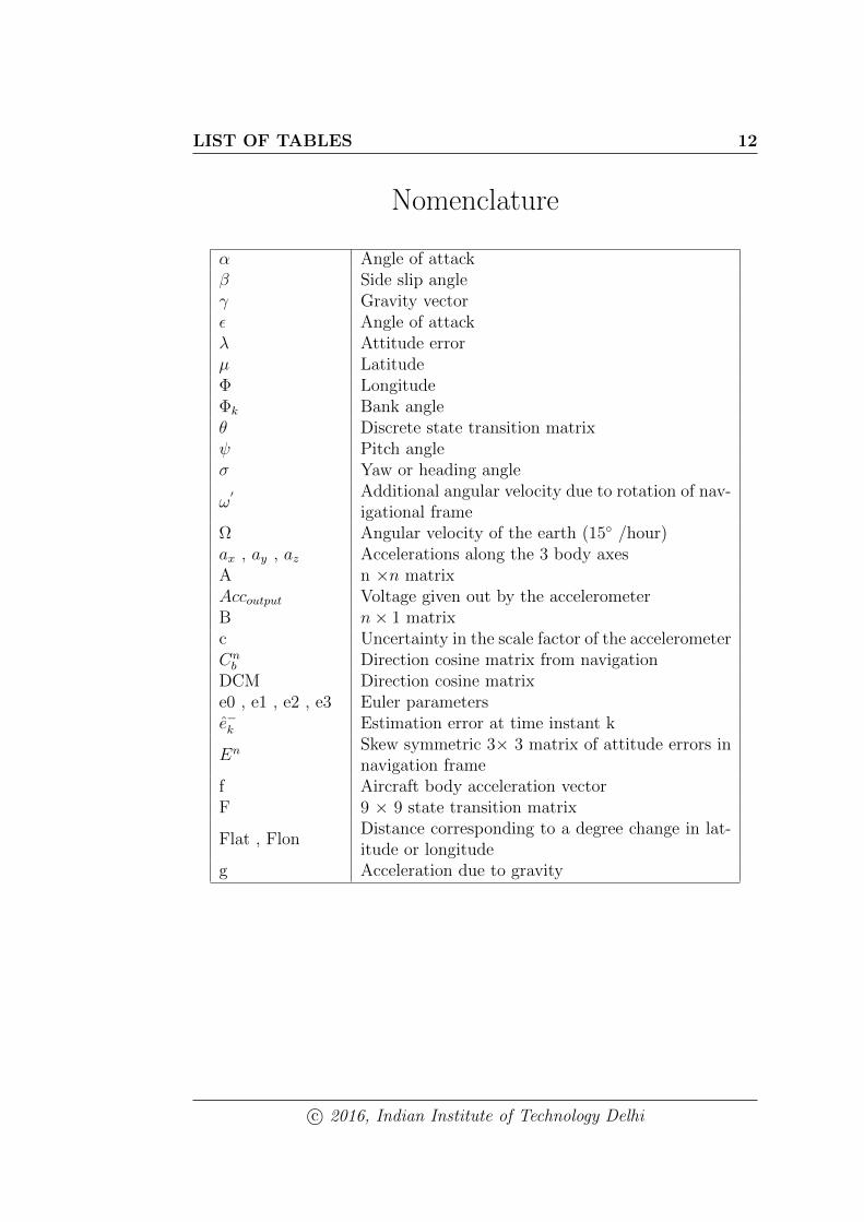
Nomenclature
α Angle of attackβ Side slip angleγ Gravity vectorε Angle of attackλ Attitude errorµ LatitudeΦ LongitudeΦk Bank angleθ Discrete state transition matrixψ Pitch angleσ Yaw or heading angle
ω′ Additional angular velocity due to rotation of nav-
igational frameΩ Angular velocity of the earth (15 /hour)ax , ay , az Accelerations along the 3 body axesA n ×n matrixAccoutput Voltage given out by the accelerometerB n× 1 matrixc Uncertainty in the scale factor of the accelerometerCn
b Direction cosine matrix from navigationDCM Direction cosine matrixe0 , e1 , e2 , e3 Euler parameterse−k Estimation error at time instant k
En Skew symmetric 3× 3 matrix of attitude errors innavigation frame
f Aircraft body acceleration vectorF 9 × 9 state transition matrix
Flat , FlonDistance corresponding to a degree change in lat-itude or longitude
g Acceleration due to gravity
c© 2016, Indian Institute of Technology Delhi
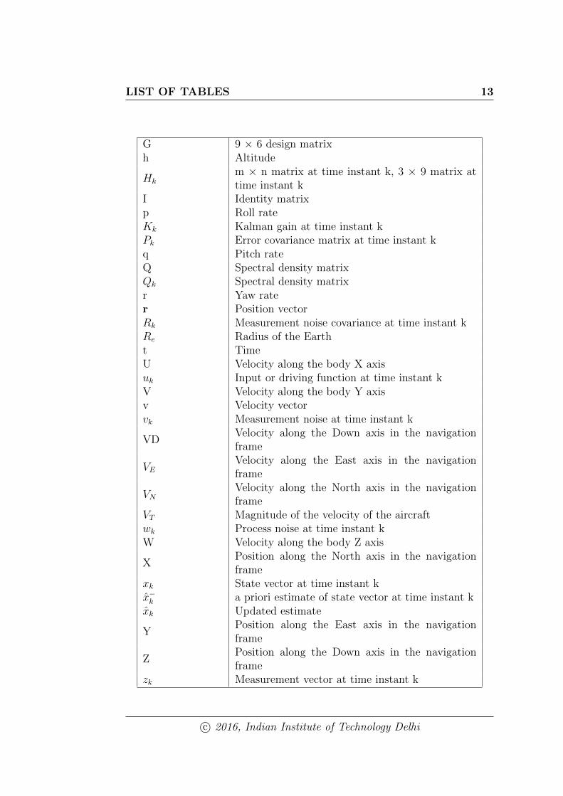
LIST OF TABLES 13
G 9 × 6 design matrixh Altitude
Hkm × n matrix at time instant k, 3 × 9 matrix attime instant k
I Identity matrixp Roll rateKk Kalman gain at time instant kPk Error covariance matrix at time instant kq Pitch rateQ Spectral density matrixQk Spectral density matrixr Yaw rater Position vectorRk Measurement noise covariance at time instant kRe Radius of the Eartht TimeU Velocity along the body X axisuk Input or driving function at time instant kV Velocity along the body Y axisv Velocity vectorvk Measurement noise at time instant k
VDVelocity along the Down axis in the navigationframe
VEVelocity along the East axis in the navigationframe
VNVelocity along the North axis in the navigationframe
VT Magnitude of the velocity of the aircraftwk Process noise at time instant kW Velocity along the body Z axis
XPosition along the North axis in the navigationframe
xk State vector at time instant kx−k a priori estimate of state vector at time instant kxk Updated estimate
YPosition along the East axis in the navigationframe
ZPosition along the Down axis in the navigationframe
zk Measurement vector at time instant k
c© 2016, Indian Institute of Technology Delhi
Chapter 1
INTRODUCTION
1.1 Mobility Assistant for Visually Impaired
(MAVI)
Mobility assistance for the visually impaired persons is of utmost importance.
This research was motivated by the problem of navigation of the visually
impaired persons in outdoor environment. The autonomous navigation is
important for people suffering from visual impairment, without depending
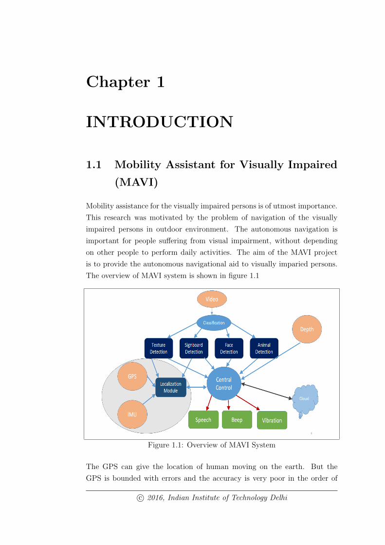
on other people to perform daily activities. The aim of the MAVI project
is to provide the autonomous navigational aid to visually imparied persons.
The overview of MAVI system is shown in figure 1.1
Figure 1.1: Overview of MAVI System
The GPS can give the location of human moving on the earth. But the
GPS is bounded with errors and the accuracy is very poor in the order of
c© 2016, Indian Institute of Technology Delhi
1.1 Mobility Assistant for Visually Impaired (MAVI) 2
20-25meters. We can not depend on the GPS for finding the location of
pedestrian accurately. To overcome this problem IMU (Inertial Measure-
ment Unit) sensor is used. The IMU gives the position and velocity of the
human but it drifts with errors due to the fact that any small bias error and
gain errors can grow with time. Hence, a position update fix is taken from
the GPS receiver module. With the help of the Kalman filter the errors in
both the IMU and the GPS is estimated and corrected to give better position
information.
There are very good advantages in designing this kind of a navigation as
compared to the ones used earlier in other systems in terms of speed and
compactness. The IMU and GPS sensors can be easily integrated with any
FPGA boards and can give effectively the position of the visually impaired
persons. With the help of MEMS technology, integration can done with high
accuracy and at lower costs and can be implemented on real-time hardware
like FPGAs.
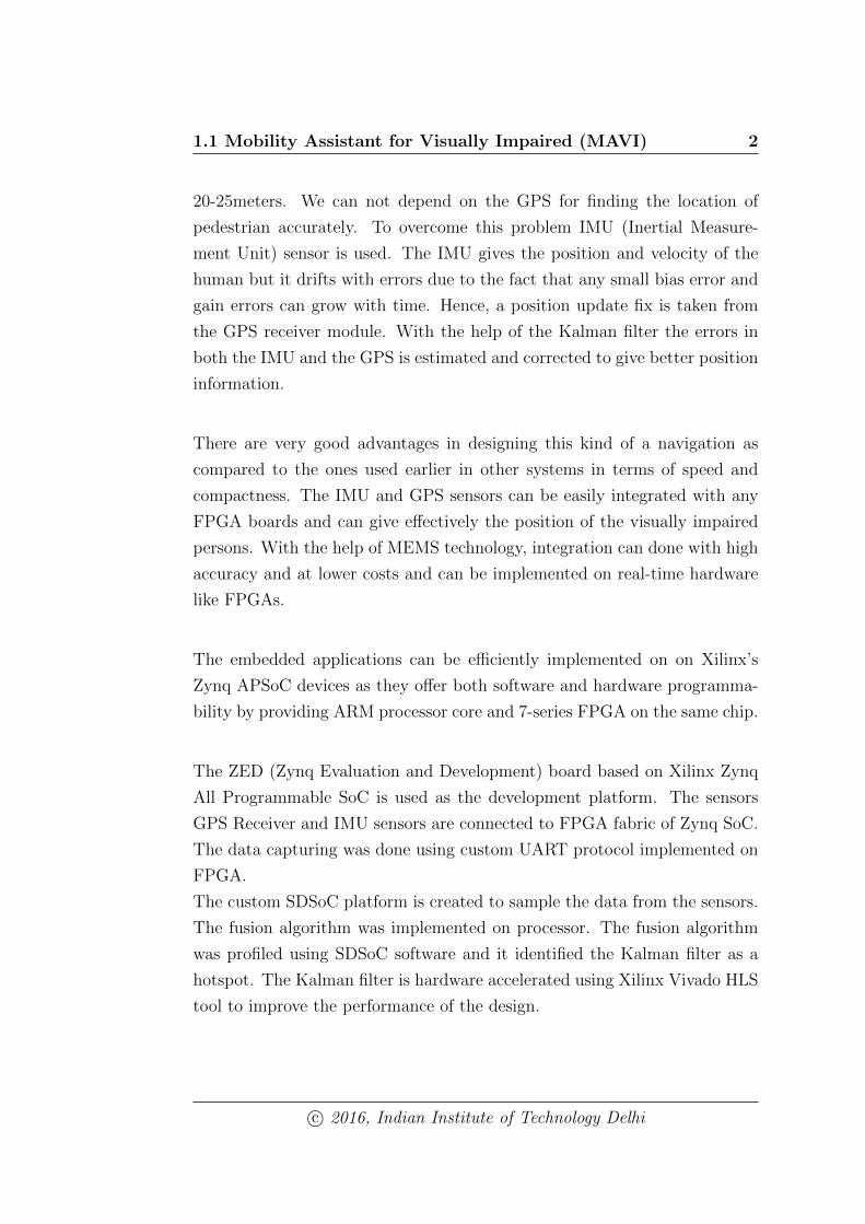
The embedded applications can be efficiently implemented on on Xilinx’s
Zynq APSoC devices as they offer both software and hardware programma-
bility by providing ARM processor core and 7-series FPGA on the same chip.
The ZED (Zynq Evaluation and Development) board based on Xilinx Zynq
All Programmable SoC is used as the development platform. The sensors
GPS Receiver and IMU sensors are connected to FPGA fabric of Zynq SoC.
The data capturing was done using custom UART protocol implemented on
FPGA.
The custom SDSoC platform is created to sample the data from the sensors.
The fusion algorithm was implemented on processor. The fusion algorithm
was profiled using SDSoC software and it identified the Kalman filter as a
hotspot. The Kalman filter is hardware accelerated using Xilinx Vivado HLS
tool to improve the performance of the design.
c© 2016, Indian Institute of Technology Delhi

1.2 Thesis Organization 3
1.2 Thesis Organization
The remaining chapters of the thesis are organized as follows:
Chapter 2: Gives a brief review of various methods of Estimation algorithms
used for sensor fusion
Chapter 3 discusses about the sensors GPS, IMU and their integration with
the Kalman filter.
Chapter 4 describes the various errors in the sensors and their calculation.
It also discusses the calibration of sensors and configuring of Register to op-
erate in various sampling rates.
Chapter 5 deals with hardware implementation. It describes the various
modules implemented in hardware and their performance
Chapter 6 describes complete custom SDSoC platform creation.
Chapter 7 deals with software implementation. It describes the various func-
tion SDSoC and SDK implementations and profiling of algorithm. It also
describes the synthesis of the Kalman filter accelerator
Chapter 8 focuses on various performance measurements
Chapter 9 conclude the thesis and gives future scope
c© 2016, Indian Institute of Technology Delhi
Chapter 2
Literature Review
There are several GPS-IMU integration techniques were implemented. Some
of them briefly described below.
Grewal et al [19]have discussed in detail in their books the working of each
of the INS, GPS and Kalman filtering in detail and have given a model of
a 54 states Kalman filter. Magnusson has discussed the sensor fusion model
based on the extended Kalman filter and inputs from a low-grade GPS re-
ceiver, IMU sensors and odometer, to improve absolute position estimation.
Vishisht Gupta [14] dissertation focused on vehicle localization using an In-
ertial Measurement Unit (IMU), GPS and a monocular camera along with
a map of the environment. The sensors used in his dissertation complement
each other to enhance the accuracy of vehicle localization in addition to
having different failure modes to increase the robustness of the system.GPS
provides the initial position required to initialize the IMU and periodically
corrects the IMU solution to estimate the accelerometer and gyroscope biases
whereas the IMU provides a fast data rate thus compensating for the slow
data rate of the GPS. Similarly, vision sensors along with a map of the envi-
ronment provide periodic corrections to the IMU solution whereas the IMU
helps the vision algorithm by predicting the location and possible variability
of the features in the map.
Maklouf [22] in his paper describes the integration of GPS with INS using
a Kalman filter in loosely coupled mode. In this integration the INS error
states, together with any navigation state (position, velocity, and attitude)
and other unknown parameters of interest, are estimated using GPS mea-
surements.
c© 2016, Indian Institute of Technology Delhi
5
Martin [18] in his thesis describes the differential GPS methods are developed
for use in automated vehicle convoy positioning. The GPS pseudo range and
carrier phase measurements are used to compute relative position vectors
between two vehicles with sub-meter errors. The carrier phase measurement
makes this level of accuracy attainable, but the carrier phase ambiguity must
be resolved prior to the relative position estimation. An algorithm, referred
to as dynamic base Real Time Kinematic (DRTK) algorithm, is described in
his thesis to estimate the carrier phase ambiguity and the relative position
vector between two GPS receivers.
Iozan [17] in their paper presents a new Hybrid Navigation System (HNS)
that combines the performances offered by inertial sensors with the ones of-
fered by the Global Navigation Satellite System(GNSS). This way the HNS
is able to estimate the 2D navigation solution even if GNSS signals are cur-
rently unavailable or intermittent. In their paper they proposed a hybrid
navigation system that combines the advantages offered by GPS and DR
(Dead Reckoning) technology. Based on this association they were able to
obtain a continuous navigation solution despite the fact that for some areas
the line-of-sight between GPS receiver and the satellites was lost.
Zhao [34] describes that the performance of the GPS/IMU integrated navi-
gation system is greatly determined by the bridging ability of the stand-alone
IMU during GPS signal outage. With better knowledge of the sensor stochas-
tic errors, we can get better estimates of the systematic errors, i.e. the bias
and drift of IMU, so that better navigation accuracy and longer bridging time
can be reached. To analyze different types of stochastic errors, they tried to
build up different stochastic models of the IMU sensors and the practical
tests on a MEMS based IMU are carried out. Although different methods
of estimating stochastic errors lead to different error models with different
coefficients, some stochastic errors of a specific sensor can be verified by com-
paring and analyzing these methods and their results. The stochastic error
models can be further used in the Kalman filter and applied in the GPS/IMU
integrated system, which is helpful for bounding the error drift during GPS
outage and the faster GPS signal reacquisition.
c© 2016, Indian Institute of Technology Delhi
Chapter 3
IMU, GPS and Kalman Filter-
ing
This section explains Inertial Navigation Systems, Reference co-ordinate
frames, GPS, Kalman Filtering. The sensors integrated are the Inertial Nav-
igation Systems. The integration of more sensors provides more accuracy
than that of the individual systems.
3.1 Inertial Measurement Unit
The IMU consists of 3-axis gyroscopes which provide the roll, pitch and
yaw about the body axes. It also consists of 3-axis accelerometers which
gives the accelerations along the three body axes. The inertial mechanism is
strap down where the gyros and accelerometers are strapped down to body
frame. The accelerometer’s, acceleration values are corrected for rotation of
the earth and gravity to give the velocity and position of the moving body.
3.2 Reference Frames and Transformations
When describing the position on or near the Earths surface, we need to de-
fine the coordinate system. The commonly used frames in inertial navigation
systems are inertial frame (i-frame), conventional terrestrial frame (e-frame),
navigation frame (n-frame) and body frame (b-frame).
Many reference frames are involved in the INS development, a vector rep-
resented in one frame must frequently be transformed into another. This
c© 2016, Indian Institute of Technology Delhi
3.2 Reference Frames and Transformations 7
section gives the various reference frames and pertaining relationships be-
tween each of them [23].
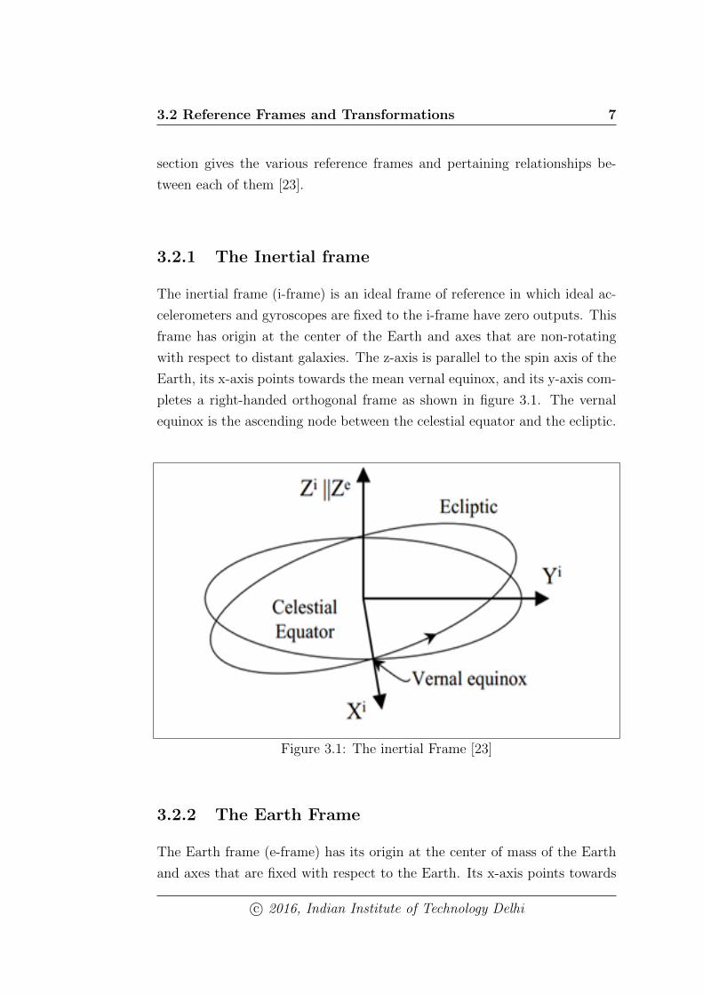
3.2.1 The Inertial frame
The inertial frame (i-frame) is an ideal frame of reference in which ideal ac-
celerometers and gyroscopes are fixed to the i-frame have zero outputs. This
frame has origin at the center of the Earth and axes that are non-rotating
with respect to distant galaxies. The z-axis is parallel to the spin axis of the
Earth, its x-axis points towards the mean vernal equinox, and its y-axis com-
pletes a right-handed orthogonal frame as shown in figure 3.1. The vernal
equinox is the ascending node between the celestial equator and the ecliptic.
Figure 3.1: The inertial Frame [23]
3.2.2 The Earth Frame
The Earth frame (e-frame) has its origin at the center of mass of the Earth
and axes that are fixed with respect to the Earth. Its x-axis points towards
c© 2016, Indian Institute of Technology Delhi
3.2 Reference Frames and Transformations 8
the mean meridian of Greenwich, its Z-axis is parallel to the mean spin axis
of the Earth, and its y-axis completes a right-handed orthogonal frame [23].
The rotation rate vector of the e-frame with respect to the i-frame projected
to the e-frame is given as
ωeie =
[0 0 ωe
]T(3.1)
Where ωe is the magnitude of the rotation rate of the Earth (7.2921158 ∗10−5rad/s)
The position vector in the e-frame can be expressed in terms of the geodetic
latitude (λ), longitude (φ), height(h) as follows
re =
x
y
z
=
(RN + h) cosφ cosλ
(RN + h) cosφ sinλ
(RN(1− e2) + h) sinφ
(3.2)
Where e is the first eccentricity of the reference ellipsoid, and RN is the ra-
dius of the curvature in the prime vertical.
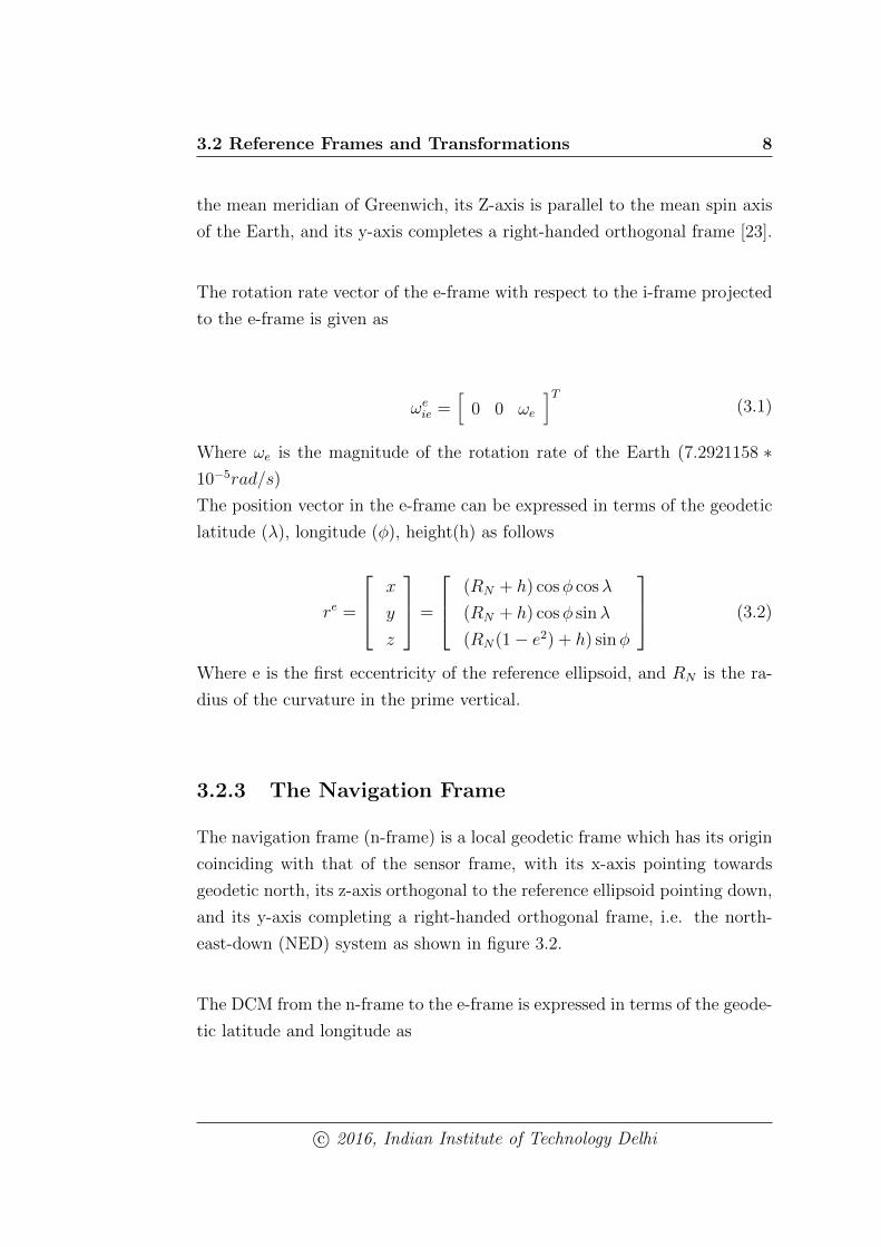
3.2.3 The Navigation Frame
The navigation frame (n-frame) is a local geodetic frame which has its origin
coinciding with that of the sensor frame, with its x-axis pointing towards
geodetic north, its z-axis orthogonal to the reference ellipsoid pointing down,
and its y-axis completing a right-handed orthogonal frame, i.e. the north-
east-down (NED) system as shown in figure 3.2.
The DCM from the n-frame to the e-frame is expressed in terms of the geode-
tic latitude and longitude as
c© 2016, Indian Institute of Technology Delhi
3.2 Reference Frames and Transformations 9
Figure 3.2: The Navigation Frame [24]
Cen =
− sinφcosλ − sinλ − cosφ cosλ
− sinφ cosλ cosλ − cosφ sinλ
cosφ 0 − sinφ
(3.3)
The quaternion corresponding to Cen is written as
qen =
cos(−π/4− φ/2) cos(λ/2)
−sin(−π/4− φ/2) sin(λ/2)
sin(−π/4− φ/2) cos(λ/2)
cos(−π/4− φ/2) sin(λ/2)
(3.4)
The Earths rotation rate can be described in the n-frame using [24]
ωnie = Cn
e ∗ ωeie
[ωe cosφ 0 −ωe ∗ sinφ
]T(3.5)
The rotation rate of the n-frame with respect to the e-frame is called the
transport rate, which can be expressed in terms of the rate of change of lat-
itude and longitude.
c© 2016, Indian Institute of Technology Delhi
3.3 Equations of Motion 10
ωnen =
·λ cosφ
−·φ
−·λ sinφ
(3.6)
Substituting·φ = vN/(RM + h) and
·λ = vE/(RN + h) cosφ into equation 3.6
yields
ωnen =
vE/(RN + h)
−vN/(RM + h)
−vE tanφ/(RN + h)
(3.7)
Where h is height; VN , VE are velocities in the north and east direction, re-
spectively; and RM is the meridian radius of curvature.
3.2.4 The Body Frame
The body frame (b-frame) is the frame in which accelerations and angular
rates generated by the strap down accelerometers and gyroscopes are re-
solved. The b-frame axes will be the same as the IMUs body axes here [24].
3.3 Equations of Motion
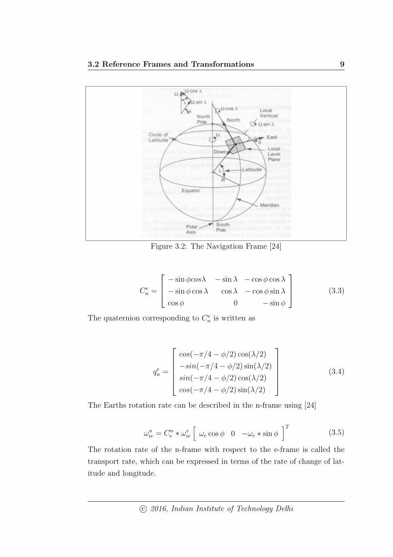
The orientation of a system with respect to a fixed inertial frame of axes is
defined by three Euler angles. The system is oriented parallel to the fixed
reference frame of axes. A series of rotations bring it to the orientation about
axes OX, OY and OZ as shown in figure 3.3 [20].
• Clockwise rotation about the yaw axis, through the yaw (or heading)
angle φ ,followed by
c© 2016, Indian Institute of Technology Delhi
3.3 Equations of Motion 11
• a clockwise rotation about the pitch axis, through the pitch angle θ,
followed by
• a clockwise rotation about the roll axis, through the bank angle ψ
Figure 3.3: Euler Angles
The relation between the gyro rates roll, pitch, yaw (p,q,r) and the Euler
angles ψ, θ, φ and their rates is given below.
·φ·θ·ψ
=
1 sinφ tan θ cosφ tan θ
0 cosφ − sinφ
0 sinφ sec θ cosφ sec θ
p
q
r
(3.8)
By integrating above equations the euler angles can be derived using the ini-
tial conditions. But the pitch angle around +/- 90 degrees tends to diverges
as tan θ tends to infinity. By using the quaternion algebra this problem can
be avoided.
The relation between Euler parameters e1, e2, e3, e4 and angular rates given by
c© 2016, Indian Institute of Technology Delhi
3.3 Equations of Motion 12
·e0 = −1
2(e1p+ e2q + e3r)
·e1 =
1
2(e0p+ e2q − e3q)
·e2 =
1
2(e0q + e3q − e1r)
·e3 =
1
2(e0r + e1q − e2p)
(3.9)
with the parameters satisfying the equation for all points of time.
e20 + e21 + e22 + e23 = 1 (3.10)
The initial values of four parameters can be calculated with the following
equations.
e0 = cosψ
2cos
θ
2cos
φ
2+ sin
ψ
2sin
θ
2sin
φ
2
e1 = cosψ
2cos
θ
2sin
φ
2− sin
ψ
2sin
θ
2cos
φ
2
e2 = cosψ
2sin
θ
2cos
φ
2+ sin
ψ
2cos
θ
2sin
φ
2
e3 = − cosψ
2sin
θ
2sin
φ
2+ sin
ψ
2cos
θ
2cos
φ
2
(3.11)
After calculating the time history of the four parameters, the Euler angles
can be calculated using the following equations.
θ = sin−1 [−2(e1e3− e0e2)] (3.12)
φ = cos−1
[e20 − e21 − e22 + e23√1− 4(e1e3 − e0e2)2
]sign [2(e2e3 + e0e1)] (3.13)
ψ = cos−1
[e20 + e21 − e22 − e23√1− 4(e1e3 − e0e2)2
]sign [2(e1e2 + e0e3)] (3.14)
The position can be calculated using the accelerations of the accelerometers.
The accelerometers gives the accelerations (ax, ay, az) along the body frame
axes. U,V,W and p,q,r are all available as states. If the acceleration due to
c© 2016, Indian Institute of Technology Delhi
3.3 Equations of Motion 13
gravity (g) model is supplied as a function of location round the earth, then·U,
·V and
·W can be calculated.
·U = aX + V r −Wq + g sin θ (3.15)
·V = aY − Ur +Wp− g cos θ sinφ (3.16)
·W = aZ + Uq − V p− g cos θ cosφ (3.17)
The earth is rotating in space at a rate Ω (15 per hour) around an axis
South to North as shown in figure 3.2.
Ω =
Ω cosλ
0
−Ω sinλ
(3.18)
The motion of the vehicle at a constant height above the ground will induce
an additional rotation given by
ω′=
.µ cosλ
−.
λ
− .µ sinλ
(3.19)
The measured angular rates include Ω and′
ω, the actual angular rates given
by p
q
r
=
p
q
r
m
−DCM[
Ω + ω′]
(3.20)
Where DCM is the the direction cosine matrix or the transformation matrix,
from navigation frame to body frame..µ is the rate of change of longitude
and.
λ is the rate of change of latitude.
c© 2016, Indian Institute of Technology Delhi
3.3 Equations of Motion 14
DCM =
cos θ cosψ cos θ sinψ − sin θ
sin θ sinφ cosψ − sinψ cosφ sinψ sin θ sinφ+ cosψ cosφ sinφ cos θ
sin θ cosφ cosψ + sinψ sinφ sinφ sin θ cosφ− cosψ sin θ cosφ cos θ
(3.21)
.
U ,.
V and.
W are integrated to calculate the velocity components (U,V, and
W) which are transformed using the direction cosine matrix to give the ve-
locity along North (VN), Velocity along East (VE) and downward velocity
(VD) in the navigation frame.
.
X.
Y.
Z
=
VN
VE
VD
= DCMT
U
V
W
(3.22)
VN ,VE and VD are then integrated to give distances moved along the naviga-
tion axes (X, Y, Z) on the surface of the earth.
Let λ, µ and H denote the latitude, longitude and height of the aircraft at
any instant, then rate of change of latitude.
λ is given by
.
λ =VNRe
(3.23)
And rate of change of longitude is given by
.µ =
VERe cosλ
(3.24)
where Re is the radius of the earth. The rate of change of altitude of the
aircraft is given by
.
H = −VD (3.25)
The position of the aircraft in terms of latitude, longitude and altitude can
be thus calculated by integrating above equations.
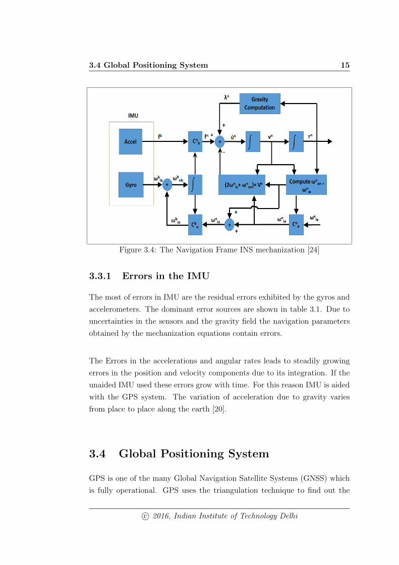
The overall navigation frame mechanization summarizes by following figure
3.4
c© 2016, Indian Institute of Technology Delhi
3.4 Global Positioning System 15
Figure 3.4: The Navigation Frame INS mechanization [24]
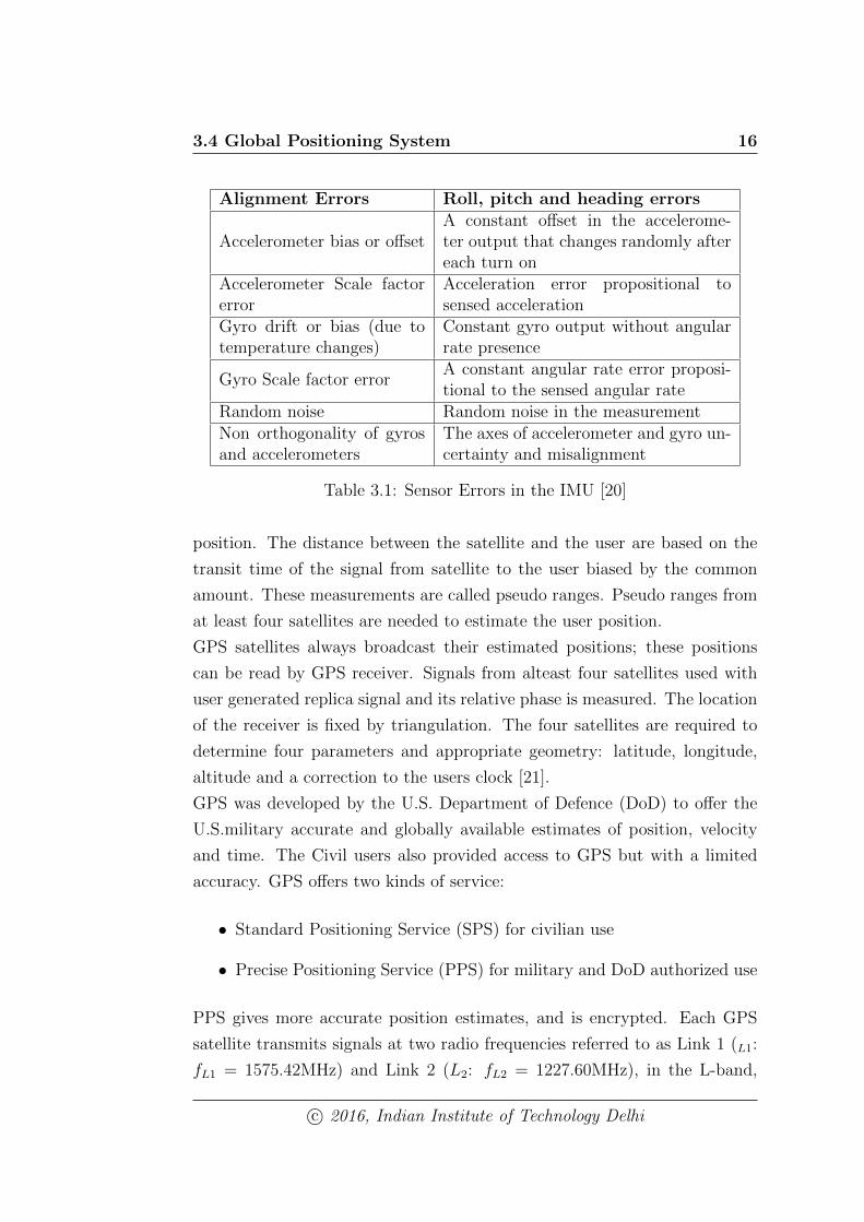
3.3.1 Errors in the IMU
The most of errors in IMU are the residual errors exhibited by the gyros and
accelerometers. The dominant error sources are shown in table 3.1. Due to
uncertainties in the sensors and the gravity field the navigation parameters
obtained by the mechanization equations contain errors.
The Errors in the accelerations and angular rates leads to steadily growing
errors in the position and velocity components due to its integration. If the
unaided IMU used these errors grow with time. For this reason IMU is aided
with the GPS system. The variation of acceleration due to gravity varies
from place to place along the earth [20].
3.4 Global Positioning System
GPS is one of the many Global Navigation Satellite Systems (GNSS) which
is fully operational. GPS uses the triangulation technique to find out the
c© 2016, Indian Institute of Technology Delhi
3.4 Global Positioning System 16
Alignment Errors Roll, pitch and heading errors
Accelerometer bias or offsetA constant offset in the accelerome-ter output that changes randomly aftereach turn on
Accelerometer Scale factorerror
Acceleration error propositional tosensed acceleration
Gyro drift or bias (due totemperature changes)
Constant gyro output without angularrate presence
Gyro Scale factor errorA constant angular rate error proposi-tional to the sensed angular rate
Random noise Random noise in the measurementNon orthogonality of gyrosand accelerometers
The axes of accelerometer and gyro un-certainty and misalignment
Table 3.1: Sensor Errors in the IMU [20]
position. The distance between the satellite and the user are based on the
transit time of the signal from satellite to the user biased by the common
amount. These measurements are called pseudo ranges. Pseudo ranges from
at least four satellites are needed to estimate the user position.
GPS satellites always broadcast their estimated positions; these positions
can be read by GPS receiver. Signals from alteast four satellites used with
user generated replica signal and its relative phase is measured. The location
of the receiver is fixed by triangulation. The four satellites are required to
determine four parameters and appropriate geometry: latitude, longitude,
altitude and a correction to the users clock [21].
GPS was developed by the U.S. Department of Defence (DoD) to offer the
U.S.military accurate and globally available estimates of position, velocity
and time. The Civil users also provided access to GPS but with a limited
accuracy. GPS offers two kinds of service:
• Standard Positioning Service (SPS) for civilian use
• Precise Positioning Service (PPS) for military and DoD authorized use
PPS gives more accurate position estimates, and is encrypted. Each GPS
satellite transmits signals at two radio frequencies referred to as Link 1 (L1:
fL1 = 1575.42MHz) and Link 2 (L2: fL2 = 1227.60MHz), in the L-band,
c© 2016, Indian Institute of Technology Delhi
3.4 Global Positioning System 17
which covers frequencies between 1 GHz and 2 GHz. Each GPS signal con-
sists of the following components:
• RF sinusoidal carrier signal with frequency fL1 and fL2
• Binary codes called pseudo-random noise (PRN) codes are modulated
on the carrier signals
For a low-cost receiver operating in autonomous mode, only L1 frequency
C/A or Clear Acquisition Code measurements are available. C/A code is
unencrypted signal broadcast at a higher bandwidth. Precise Code is broad-
cast at a higher bandwidth and is restricted for military use. The C/A code
is intentionally degraded the accuracy by introducing the clock jitter and
is known as Selective Availability. Errors of 100m can exist with selective
availability. There are six major causes of ranging errors: Satellite ephemeris,
Satellite clock, tropospheric group delay, ionospheric group delay, multipath
and receiver measurement errors.
3.4.1 Limitations and Errors in GPS
In order to pinpoint a location using GPS atleast four or more satellites in-
formation is needed. If the no of visible satellites are lesser than four, the
receiver can′t estimate its position. If the no of visible satellites more than
four then the measurement accuracy improved. This means the system is
more robust to disturbances in the signals received [21].
Errors in the position measurement can originates either from transmitted
satellite, during signal propagation or in the receiver. There many errors
and biases that affect the GPS system from satellite to receiver viz., Clock
error, relativistic effects, orbital error, ionospheric and tropospheric delay,
multipath error and instrumental biases.
Even though, each GPS satellite has four atomic clocks on board, there will
be always a small timing error. When a satellite moves out of orbit then the
orbital error occurs, this needs to be corrected. Relativity is affecting the
GPS system by changing orbital position due to earth gravitation field, the
c© 2016, Indian Institute of Technology Delhi
3.5 Sensor Fusion Theory 18
satellite clock frequency is influenced by the gravitational field.
The GPS signals travels through ionosphere and troposphere which creates
the delay in the signal received by receiver. The ionosphere delay is mea-
sured and corrected. But the tropospheric delay depends on temperature,
air pressure and humidity which are difficult to estimate and hence affects
the measurement accuracy.
Multipath errors occurs due to reception of one or more reflections of same
GPS signal, caused by the surroundings such as buildings, trucks or large ob-
jects. These multipath errors can be attenuated by the use of Right-Handed
Circularly Polarized (RHCP) antennas and another method that uses the
Signal to Noise Ratio(SNR). One more method is to use a so-called choke
ring antenna, which reflects signals coming from shallow angles. However the
best method is keep the receiver in outer space where the risk of reflections
reduced.
Large structures not only create the multipath errors and also block the sig-
nals. The signal blocking is most common in urban areas.
3.5 Sensor Fusion Theory
The goal of sensor fusion is to combine the measurements from different sen-
sors to improve the quality of the information, as the combined information
is more valuable than individual sensor. The sensor fusion is divided into
following categories; fusion across sensors, fusion across attributes, fusion
across domains and fusion across time.
Fusion across sensors is when several sensors measure the same attribute eg:
velocity of vehicle, which improves the robustness of measured data. Fusion
across attributes is when several sensors measure the different attributes, e.g.
c© 2016, Indian Institute of Technology Delhi
3.5 Sensor Fusion Theory 19
acceleration, position and angular velocity. This kind improves the value of
the data by combining information from different sources. Fusion across do-
mains measures same attribute but at different range., e.g. cold and warm
ranged temperature sensors. The sensor fusion across time where the same
attribute is measured at different times, which could increase reliability of a
measurement [21].
Another way of sensor fusion is divided into three parts; complementary,
competitive and cooperative. In Complementary fusion, the independent
sensors measures different parts of the system to obtain whole system infor-
mation. In competitive fusion, different sensors measures same attribute to
make the system more robust. Finally in cooperative fusion, a combination
of the sensors obtains information, which could not be possible with single
sensor.
3.5.1 Kalman Filter
A Kalman filtering is a recursive filtering method which used frequently in
sensor fusion for discrete data, developed by Rudolph Kalman and published
in 1960. The Kalman filter estimates the past, present and future states of
linear systems by using measurements in a fashion that minimizes the least
mean squared error (LMSE). Kalman Filter minimizes the variance between
the prediction of parameters from a previous time instant and external ob-
servations at a present time instant.
In order to deal with nonlinear systems, the Extended Kalman filter (EKF)
which is linearized around a working point is used. In most of the sensor
fusion applications the Kalman Filter is used due to its computational effi-
ciency. Following equations describes the Kalman Filter [21].
The states, x ε Rn, are a part of a linear discrete time process described below
c© 2016, Indian Institute of Technology Delhi
3.5 Sensor Fusion Theory 20
xk = Axk−1 +BUk−1 + wk−1 (3.26)
Where
Matrix A ε Rnxn relates the state x from time step k-1 to k, and can be
either constant or changing in time. The matrix A is often referred to as the
process model of the Kalman filter.
Matrix B ε Rnx1 relates the control input u to the states from time step k-1
to k, and can be either constant or changing in time.
Vector u ε Rl is the control input, which is optional.
Vector w ε Rn is a random variable representing the process noise of the sys-
tem, which is assumed to be white and normally distributed, w ∼ N(0, Q),
where Q is the process noise covariance matrix that can be either constant
or changing in time.
The states x are effected by measurements z ε Rmthat, e.g., can be data from
sensor outputs.
Zk = Hxk + vk (3.27)
Where
Matrix H ε Rmxn relates the state x from time step from k to measurements
z at time step k, and can be either constant or changing in time. The matrix
H is often referred to as the measurement model of the Kalman filter.
Vector v ε Rn is a random variable representing the measurement noise of
the system, which is assumed to be white and normally distributed, v ∼ N(0,
R), where R is the measurement noise covariance matrix that can be either
constant or changing in time.
First the Kalman filter calculates a primary priori estimate of process infor-
c© 2016, Indian Institute of Technology Delhi
3.5 Sensor Fusion Theory 21
mation of step k- x−k and then calculate a final priori estimate of the state
for given measurement Zk at time step k— xk
An initial estimate of the process at time instant tk assumed, and this es-
timate is based on process prior to tk. The prior estimate is denoted by
x−k , where hat denotes its estimate and minus denotes its previous best esti-
mate [20].
The estimate error can be define as
ek = xk − xk (3.28)
and the covariance matrix as
P−k = E[(e−k )(e−k )T
]= E
[(xk − x−k )(xk − x−k )
](3.29)
The assumed prior estimate can be improved with the help Zk by the follow-
ing equation
xk = x−k +Kk(zk −Hx−k ) (3.30)
where the updated estimate xk and Kk is the Kalman Gain which minimizes
a posteriori error covariance
Substituting equation 3.26 into 3.32 and then substituting the resulting ex-
pression into 3.33 we get
Pk = (I −KkHk)P−k (3.31)
The Kalman gain which reduces the mean square error can be given by
Kk = P−k HT (HP−k H
T +R)−1 (3.32)
The measurement error R decreases, the Kalman gain will increase and the
estimate dependents more on measurement. When a priori estimate error Pk
decreases, the Kalman gain will decrease and the Kalman filter output rely
on the priori estimate.
The next estimated step measurement x−k+1, the error covariance P−k+1 and
c© 2016, Indian Institute of Technology Delhi
3.5 Sensor Fusion Theory 22
the process repeats.
x−k+1 = Akxk +Bkuk (3.33)
P−k+1 = AkPkATk +Qk (3.34)
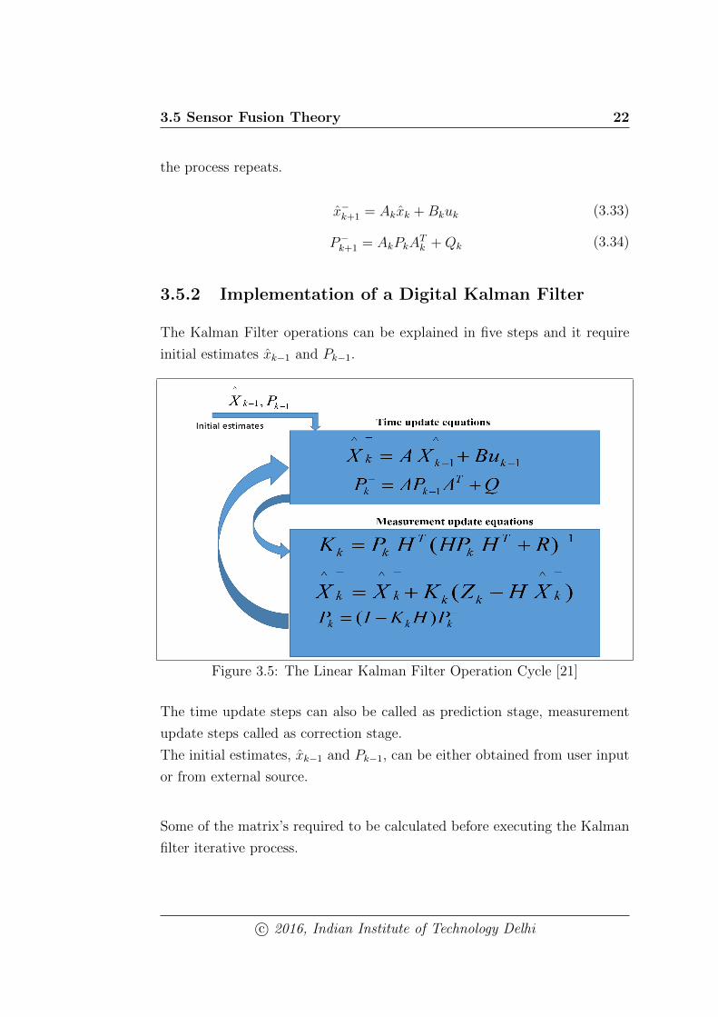
3.5.2 Implementation of a Digital Kalman Filter
The Kalman Filter operations can be explained in five steps and it require
initial estimates xk−1 and Pk−1.
Figure 3.5: The Linear Kalman Filter Operation Cycle [21]
The time update steps can also be called as prediction stage, measurement
update steps called as correction stage.
The initial estimates, xk−1 and Pk−1, can be either obtained from user input
or from external source.
Some of the matrix’s required to be calculated before executing the Kalman
filter iterative process.
c© 2016, Indian Institute of Technology Delhi
3.5 Sensor Fusion Theory 23
state transformation matrix A,
the optional control input transformation matrix B,
measurement noise covariance matrix R,
process noise covariance matrix Q,
and the state to measurement transformation matrix H.
the state transformation matrix A includes, both the state in x and its pre-
vious state xk−1 which together forms the current state xk. Depending on
the type of system u the control input will exists. In sensor fusion if there is
no direct control action then there is no need of control matrix u and matrix
B. The measurement noise covariance matrix R, which is calculated offline,
its depends upon the environment where the sensor data is captured. The
Rk matrix either updated iteratively or through user input. The state to
measurement transformation matrix H, it needs relationship between state
and measurement.
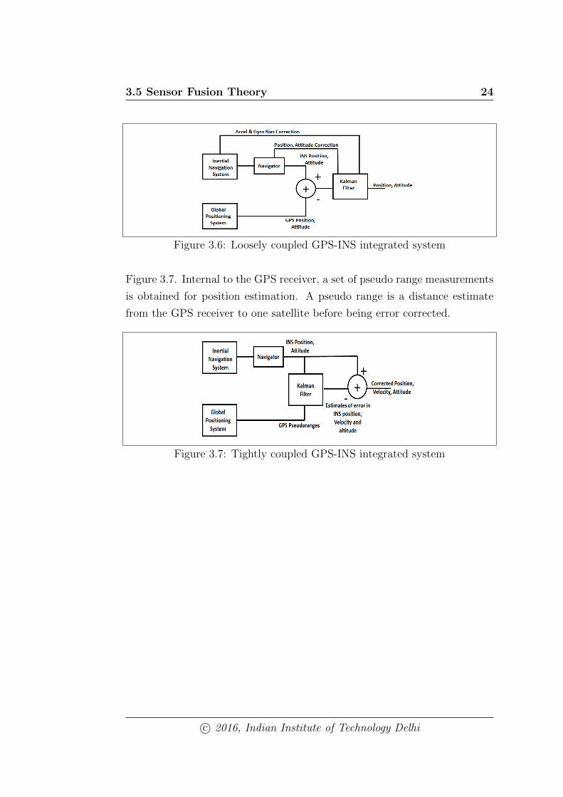
3.5.3 GPS/IMU integration
There are many methods to integrate GPS data with the IMU data. These
includes loosely, tightly and even ultra-tightly.
In case of loosely coupled approach, the GPS data is extracted at the latest
stage of processing within the GPS receiver. i.e. the position, velocity, al-
titude. The tightly coupled approach, the GPS data is extracted as pseudo
range, carrier phase and Doppler measurements. In case of ultra-tightly cou-
pled approach, data fetching done early and apart from having pseudo range,
carrier phase and Doppler measurements there is feedback Doppler estimates
to GPS receiver [21].
Each of integration method has their advantages and disadvantages. The
loosely coupled approach is relatively simple to implement but has the prob-
lem of not computing the position due to limited satellite visibility but this
problem is avoided by tightly coupled approach.
The block diagram of a tightly coupled integration technique is shown in
c© 2016, Indian Institute of Technology Delhi
3.5 Sensor Fusion Theory 24
Figure 3.6: Loosely coupled GPS-INS integrated system
Figure 3.7. Internal to the GPS receiver, a set of pseudo range measurements
is obtained for position estimation. A pseudo range is a distance estimate
from the GPS receiver to one satellite before being error corrected.
Figure 3.7: Tightly coupled GPS-INS integrated system
c© 2016, Indian Institute of Technology Delhi
Chapter 4
Sensor Characterization
4.1 GPS
The GPS module used in project was SIM28, which is a stand-alone GPS
receiver. The SIM28 has low power consumption (acquisition 24mA, tracking
19mA) [25,26] .
4.1.1 Key Features
The communication with the sensor will be in NMEA message format. The
module operates on 2.8V-4.3V power supply.The I/O data levels are 2.8V
CMOS compatible [25].
• Interface
– UART
– SPI/I2C
• Operating Temperature: -40 — +85 C
• Accuracy 2.5m CEP
4.2 IMU
The IMU sensor used is 9 Degrees of Freedom- Razor IMU. It has three
sensors- an ITG-3200 (MEMS triple-axis gyro), HMC5883L (triple-axis mag-
netometer) and ADXL345 (triple axis accelerometer).The sensor data is pro-
cessed by a micro controller ATmega328 and output over UART or SPI/I2C
c© 2016, Indian Institute of Technology Delhi
4.2 IMU 26
serial interfaces. It operates with 3.3VDC supply [1].
The IMU data was captured from the sensors through UART at 57600bps
data rate. The data was sampled from individual sensors i.e. Accelerometer,
Gyroscope and magnetometer at various sampling rates.
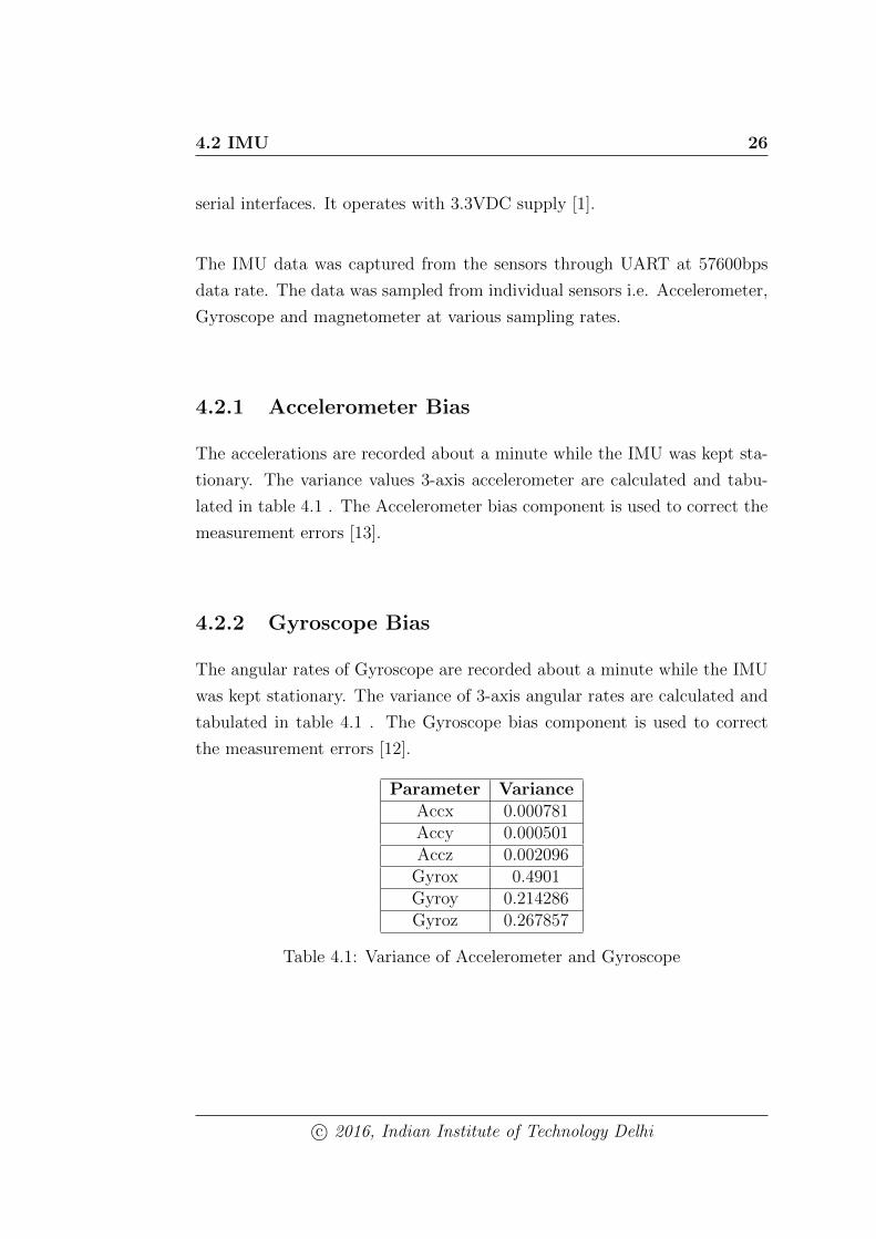
4.2.1 Accelerometer Bias
The accelerations are recorded about a minute while the IMU was kept sta-
tionary. The variance values 3-axis accelerometer are calculated and tabu-
lated in table 4.1 . The Accelerometer bias component is used to correct the
measurement errors [13].
4.2.2 Gyroscope Bias
The angular rates of Gyroscope are recorded about a minute while the IMU
was kept stationary. The variance of 3-axis angular rates are calculated and
tabulated in table 4.1 . The Gyroscope bias component is used to correct
the measurement errors [12].
Parameter VarianceAccx 0.000781Accy 0.000501Accz 0.002096
Gyrox 0.4901Gyroy 0.214286Gyroz 0.267857
Table 4.1: Variance of Accelerometer and Gyroscope
c© 2016, Indian Institute of Technology Delhi
4.3 Calibration using Arduino 27
4.3 Calibration using Arduino
The individual sensors of IMU is required to be calibrated before actual us-
ing. The calibration improves sensors performance by removing its structural
errors. These errors are difference in measured and expected outputs. The
sensor should be powered on few minutes before the calibration so that the
sensor can warm up.
The sensors accelerometer, gyroscope and magnetometer can be calibrated
by the standard procedure given in [2]. The calibrated values are obtained
by calibration and are updated.
4.4 Configuration Registers of IMU
The individual sensors can be programmed for different sampling rates by
configuring the specified registers.
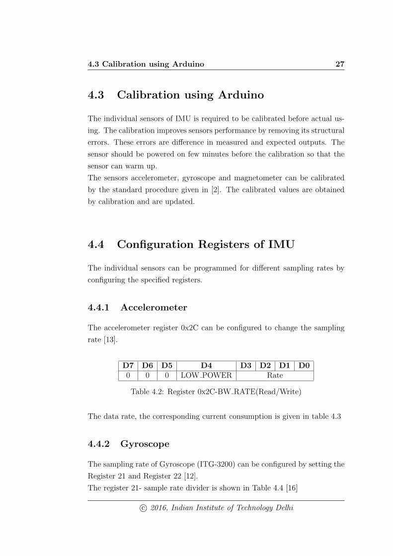
4.4.1 Accelerometer
The accelerometer register 0x2C can be configured to change the sampling
rate [13].
D7 D6 D5 D4 D3 D2 D1 D00 0 0 LOW POWER Rate
Table 4.2: Register 0x2C-BW RATE(Read/Write)
The data rate, the corresponding current consumption is given in table 4.3
4.4.2 Gyroscope
The sampling rate of Gyroscope (ITG-3200) can be configured by setting the
Register 21 and Register 22 [12].
The register 21- sample rate divider is shown in Table 4.4 [16]
c© 2016, Indian Institute of Technology Delhi
4.4 Configuration Registers of IMU 28
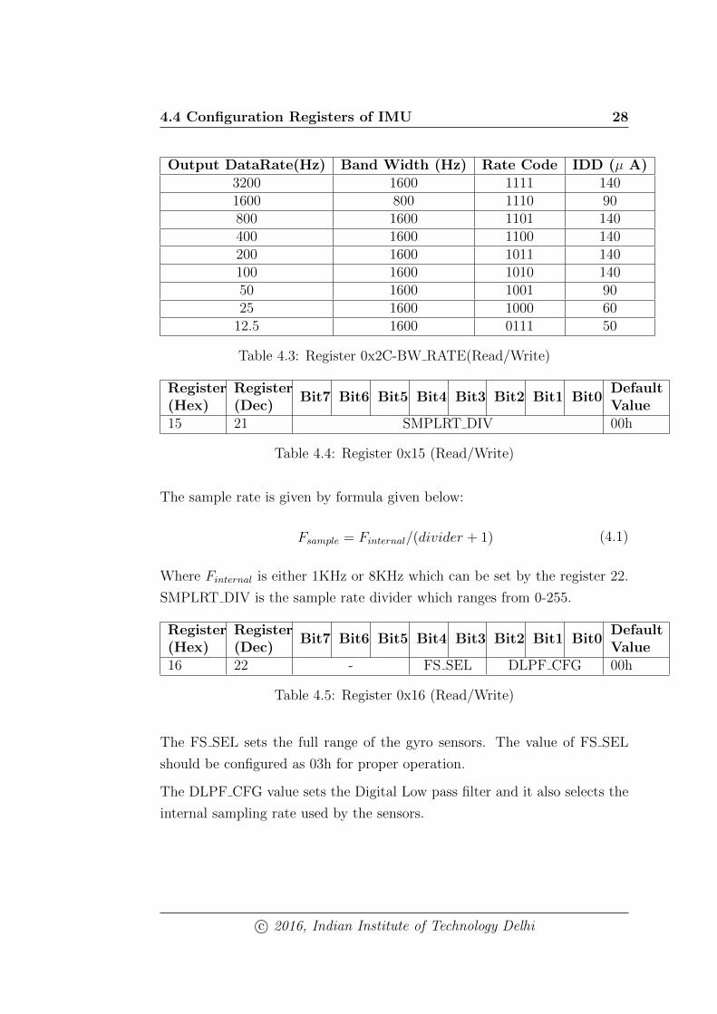
Output DataRate(Hz) Band Width (Hz) Rate Code IDD (µ A)3200 1600 1111 1401600 800 1110 90800 1600 1101 140400 1600 1100 140200 1600 1011 140100 1600 1010 14050 1600 1001 9025 1600 1000 60
12.5 1600 0111 50
Table 4.3: Register 0x2C-BW RATE(Read/Write)
Register(Hex)
Register(Dec)
Bit7 Bit6 Bit5 Bit4 Bit3 Bit2 Bit1 Bit0DefaultValue
15 21 SMPLRT DIV 00h
Table 4.4: Register 0x15 (Read/Write)
The sample rate is given by formula given below:
Fsample = Finternal/(divider + 1) (4.1)
Where Finternal is either 1KHz or 8KHz which can be set by the register 22.
SMPLRT DIV is the sample rate divider which ranges from 0-255.
Register(Hex)
Register(Dec)
Bit7 Bit6 Bit5 Bit4 Bit3 Bit2 Bit1 Bit0DefaultValue
16 22 - FS SEL DLPF CFG 00h
Table 4.5: Register 0x16 (Read/Write)
The FS SEL sets the full range of the gyro sensors. The value of FS SEL
should be configured as 03h for proper operation.
The DLPF CFG value sets the Digital Low pass filter and it also selects the
internal sampling rate used by the sensors.
c© 2016, Indian Institute of Technology Delhi
4.4 Configuration Registers of IMU 29
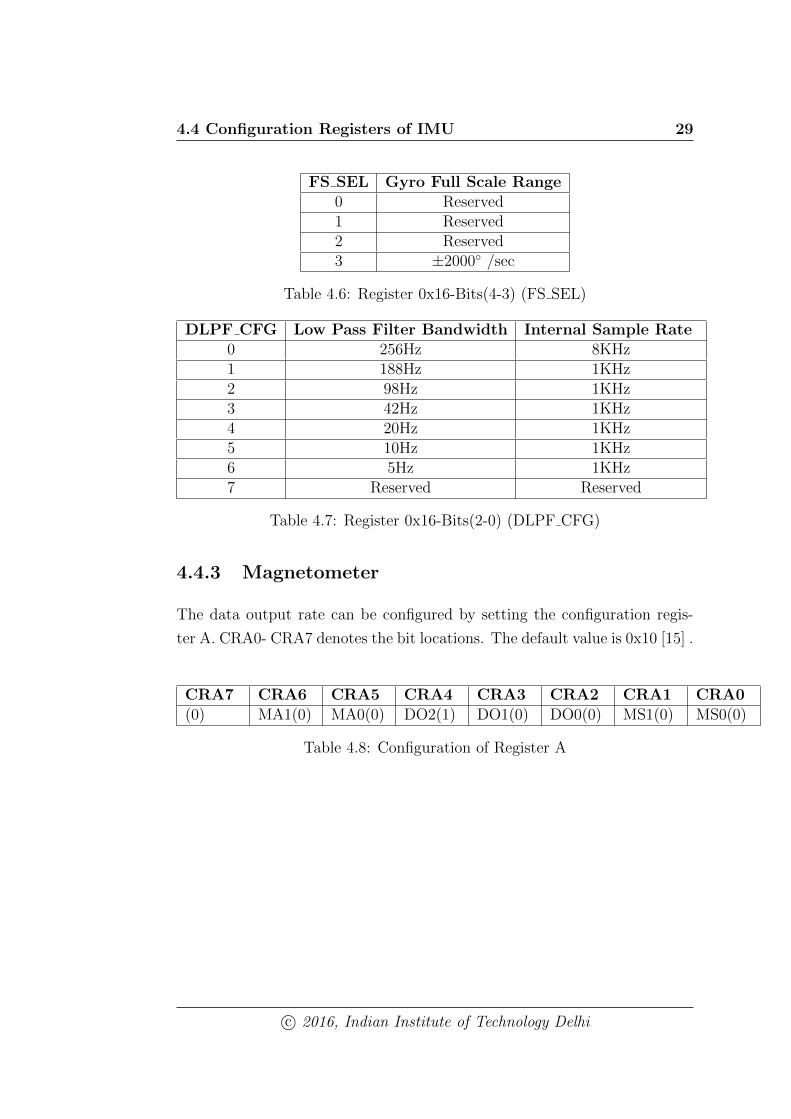
FS SEL Gyro Full Scale Range0 Reserved1 Reserved2 Reserved3 ±2000 /sec
Table 4.6: Register 0x16-Bits(4-3) (FS SEL)
DLPF CFG Low Pass Filter Bandwidth Internal Sample Rate0 256Hz 8KHz1 188Hz 1KHz2 98Hz 1KHz3 42Hz 1KHz4 20Hz 1KHz5 10Hz 1KHz6 5Hz 1KHz7 Reserved Reserved
Table 4.7: Register 0x16-Bits(2-0) (DLPF CFG)
4.4.3 Magnetometer
The data output rate can be configured by setting the configuration regis-
ter A. CRA0- CRA7 denotes the bit locations. The default value is 0x10 [15] .
CRA7 CRA6 CRA5 CRA4 CRA3 CRA2 CRA1 CRA0(0) MA1(0) MA0(0) DO2(1) DO1(0) DO0(0) MS1(0) MS0(0)
Table 4.8: Configuration of Register A
c© 2016, Indian Institute of Technology Delhi

4.4 Configuration Registers of IMU 30
Location Name Description
CRA7 CRA7Bit CRA7 is reserved for futurefunction. Set to 0 when configur-ing CRA
CRA6 to CRA5 MA1 to MA0
Select number of samplesaveraged (1-8) per mea-surement output. 00=1(De-fault);01=2;10=4;11=8
CRA4 to CRA2 DO2 to DO0
Data Output Rate Bits. Thesebits set the rate at which data iswritten to all three data outputregisters.
CRA1 to CRA0 MS1 to MS0
Measurement Configuration Bits.These bits define the measure-ment flow of the device, specifi-cally whether or not to incorpo-rate an applied bias into the mea-surement.
Table 4.9: Configuration of Register A Bit Designations
c© 2016, Indian Institute of Technology Delhi
Chapter 5
Hardware Implementation
5.1 Overview
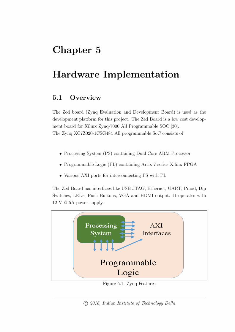
The Zed board (Zynq Evaluation and Development Board) is used as the
development platform for this project. The Zed Board is a low cost develop-
ment board for Xilinx Zynq-7000 All Programmable SOC [30].
The Zynq XC7Z020-1CSG484 All programmable SoC consists of
• Processing System (PS) containing Dual Core ARM Processor
• Programmable Logic (PL) containing Artix 7-series Xilinx FPGA
• Various AXI ports for interconnecting PS with PL
The Zed Board has interfaces like USB-JTAG, Ethernet, UART, Pmod, Dip
Switches, LEDs, Push Buttons, VGA and HDMI output. It operates with
12 V @ 5A power supply.
Figure 5.1: Zynq Features
c© 2016, Indian Institute of Technology Delhi
5.2 Architecture 32
5.2 Architecture
5.2.1 Processing System
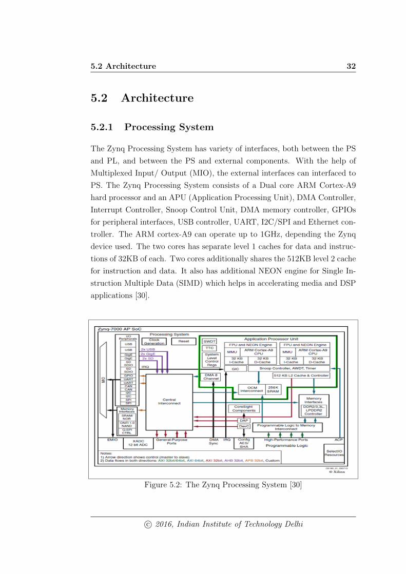
The Zynq Processing System has variety of interfaces, both between the PS
and PL, and between the PS and external components. With the help of
Multiplexed Input/ Output (MIO), the external interfaces can interfaced to
PS. The Zynq Processing System consists of a Dual core ARM Cortex-A9
hard processor and an APU (Application Processing Unit), DMA Controller,
Interrupt Controller, Snoop Control Unit, DMA memory controller, GPIOs
for peripheral interfaces, USB controller, UART, I2C/SPI and Ethernet con-
troller. The ARM cortex-A9 can operate up to 1GHz, depending the Zynq
device used. The two cores has separate level 1 caches for data and instruc-
tions of 32KB of each. Two cores additionally shares the 512KB level 2 cache
for instruction and data. It also has additional NEON engine for Single In-
struction Multiple Data (SIMD) which helps in accelerating media and DSP
applications [30].
Figure 5.2: The Zynq Processing System [30]
c© 2016, Indian Institute of Technology Delhi
5.2 Architecture 33
5.2.2 Programmable Logic
The PL predominantly composed of general purpose Artix 7 FPGA logic fab-
ric which composed of slices, CLBs (Configuration Logic Blocks) and Input/
Output Blocks (IOBs) for interfacing.
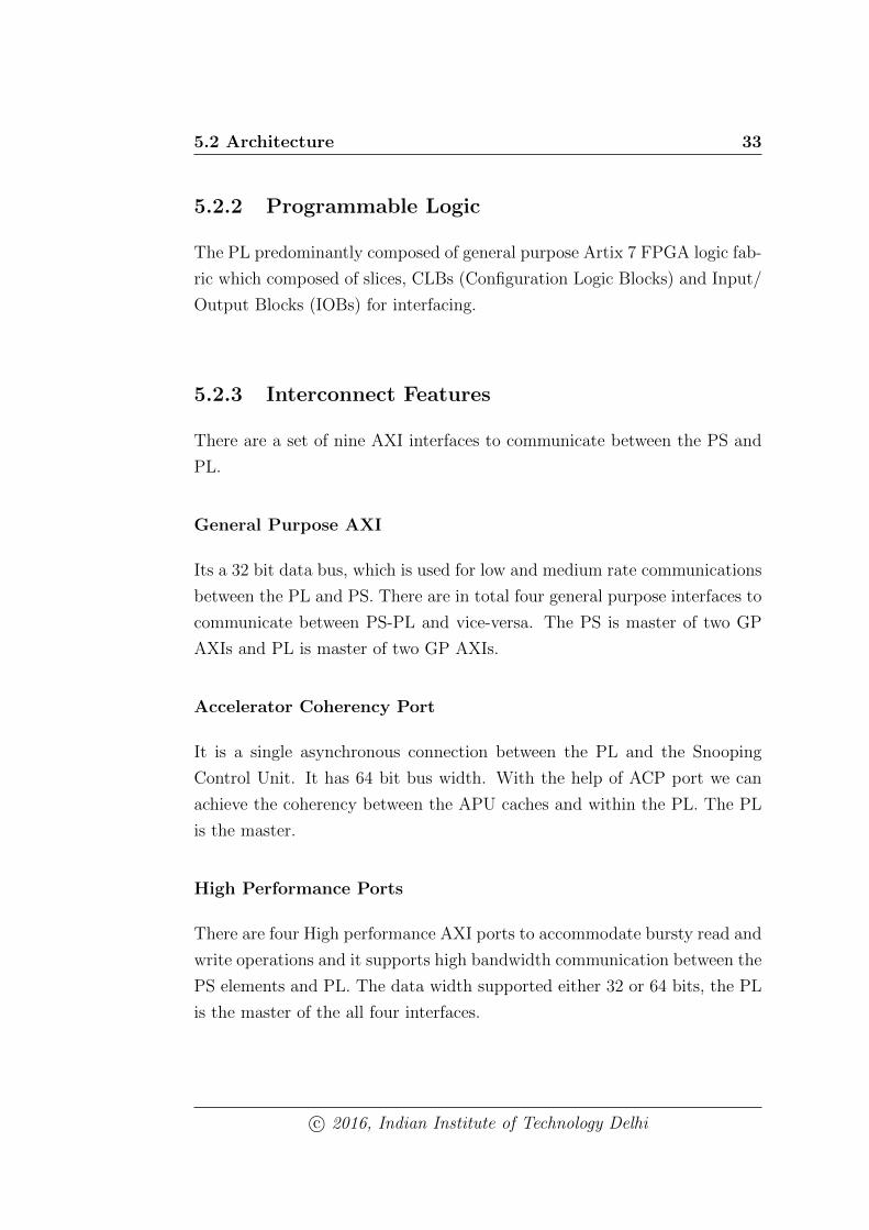
5.2.3 Interconnect Features
There are a set of nine AXI interfaces to communicate between the PS and
PL.
General Purpose AXI
Its a 32 bit data bus, which is used for low and medium rate communications
between the PL and PS. There are in total four general purpose interfaces to
communicate between PS-PL and vice-versa. The PS is master of two GP
AXIs and PL is master of two GP AXIs.
Accelerator Coherency Port
It is a single asynchronous connection between the PL and the Snooping
Control Unit. It has 64 bit bus width. With the help of ACP port we can
achieve the coherency between the APU caches and within the PL. The PL
is the master.
High Performance Ports
There are four High performance AXI ports to accommodate bursty read and
write operations and it supports high bandwidth communication between the
PS elements and PL. The data width supported either 32 or 64 bits, the PL
is the master of the all four interfaces.
c© 2016, Indian Institute of Technology Delhi
5.3 UART 34
5.2.4 AXI Interconnect Types
There are 3 flavours of AXI (Advanced Extensible Interfaces) Standards.
• AXI4: It is a memory mapped interface. An address is supplied fol-
lowed by data burst of size upto 256 data words.
• AXI4-Lite: A simplified link supporting only one data transfer per
connection. AXI4-Lite is also memory mapped but only one address
and single data word is transferred.
• AXI4-streaming: For transferring high speed streaming data of unre-
stricted size it will be used. There is no address mechanism. This type
of bus is best suited to direct data flow between source and destination.
Figure 5.3: The Interconnect Features [30]
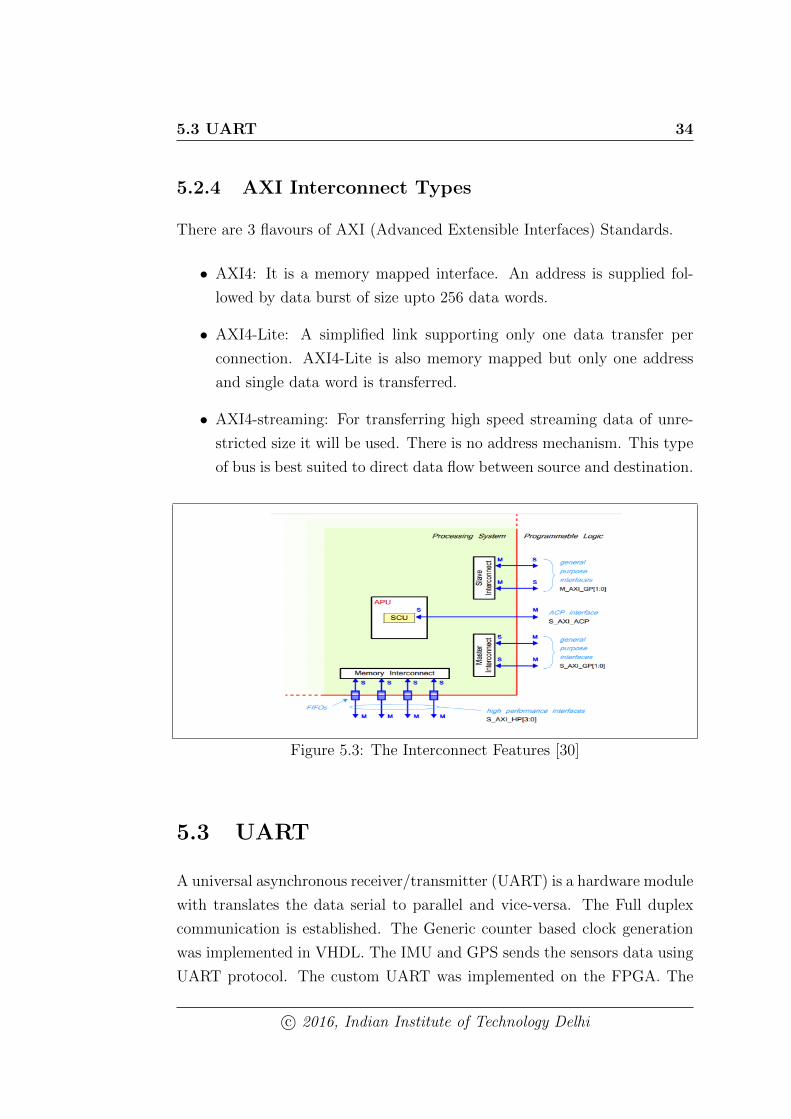
5.3 UART
A universal asynchronous receiver/transmitter (UART) is a hardware module
with translates the data serial to parallel and vice-versa. The Full duplex
communication is established. The Generic counter based clock generation
was implemented in VHDL. The IMU and GPS sends the sensors data using
UART protocol. The custom UART was implemented on the FPGA. The
c© 2016, Indian Institute of Technology Delhi
5.3 UART 35
GPS and IMU sensors were connected to FPGA through PMOD connector
User I/O s. The GPS sends the data at 9600 bps rate and IMU sends the
data at 57600 bps rate. The two different UARTs were implemented and
used.
Figure 5.4: UART Input/Ouput Ports
Resource Utilization
The following table 5.1 shows the resource utilization of UART module im-
plemented.
Resource UtilizationSlice Registers 72(≈ 0%)Slice LUTs 133(≈ 0%)DSP48E1 0(≈ 0%)BUFG/BUFGCTRLs 2(≈ 6%)
Table 5.1: UART Resource Utilization
c© 2016, Indian Institute of Technology Delhi
5.4 Co-ordinate Conversion 36
5.4 Co-ordinate Conversion
5.4.1 System Generator
The GPS gives the data in Longitude, latitude format. This data needs to
convert into Cartesian coordinates, which will be used in the algorithm. The
coordinate conversion algorithm was implemented using Xilinx System Gen-
erator [31] tool. The system generator is the industrys leading high level tool
for designing high performance DSP systems using Xilinx All Programmable
FPGAs. The co-ordinate conversion was verified by simulating using system
generator tool. The VHDL net list files were generated by the System Gen-
erator tool. The net list files were synthesized using the Xilinx ISE tool. The
three different data types of implementation were done. i.e. Fixed Point,
Single-Precision Floating Point , Double Precision Floating Point.
5.4.2 Fixed Point Implementation
The 32 bit fixed point implementation is used. The appropriate binary point
was selected at all stages of conversion.
5.4.3 Single Point Implementation
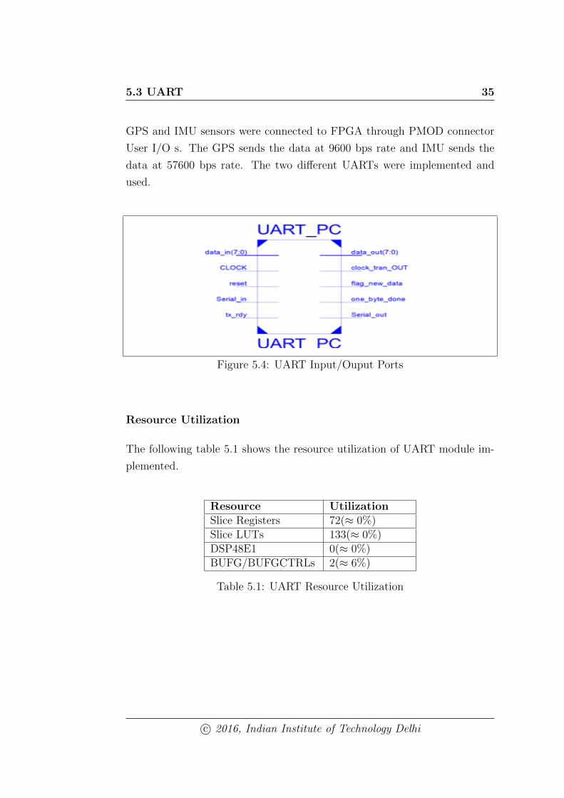
Single-Precision floating point format uses 32bit IEEE 754-2008 [8]. It has
wider range over fixed point of same bit-width. The IEEE 754 standard
specifies a binary32 as
• Sign bit : 1bit
• Exponenet width: 8 bits
• Significand precision:24 bits
c© 2016, Indian Institute of Technology Delhi

5.4 Co-ordinate Conversion 37
Figure 5.5: Single Precision Floating Point Representation
5.4.4 Double Precision Floating Point
Double-precision floating point used due its wider range over single-precision
floating point [4]. The IEEE 754 standard specifies a binary64 as having
• Sign bit : 1bit
• Exponenet width: 11 bits
• Significand precision:53 bits
Figure 5.6: Double Precision Floating Point Representation
The three implementation were implemented on Zynq FPGA and the imple-
mentation results are given below.
Resource Fixed PointSingle-PrecisionFloat
Double-PrecisionFloat
Slice Registers 20370(≈ 19%) 15634(≈ 14%) 16206(≈ 15%)Slice LUTs 20737(≈ 38%) 21752(≈ 33%) 29653(≈ 55%)DSP48E1 80(≈ 36%) 42(≈ 19%) 196(≈ 89%)BUFG/BUFGCTRLs 1(≈ 3%) 1(≈ 3%) 1(≈ 3%)
Table 5.2: Co-ordinate Conversion Resource Utilization
c© 2016, Indian Institute of Technology Delhi
5.5 Data capture module for GPS 38
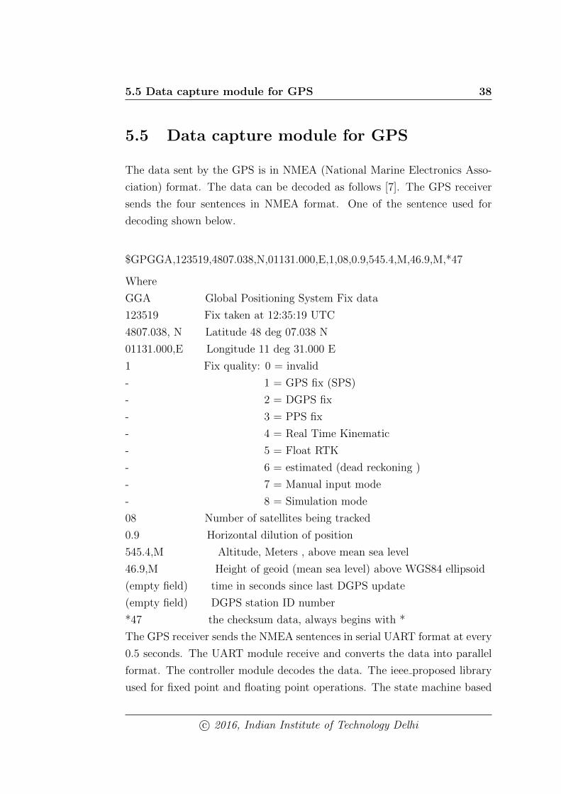
5.5 Data capture module for GPS
The data sent by the GPS is in NMEA (National Marine Electronics Asso-
ciation) format. The data can be decoded as follows [7]. The GPS receiver
sends the four sentences in NMEA format. One of the sentence used for
decoding shown below.
$GPGGA,123519,4807.038,N,01131.000,E,1,08,0.9,545.4,M,46.9,M,*47
Where
GGA Global Positioning System Fix data
123519 Fix taken at 12:35:19 UTC
4807.038, N Latitude 48 deg 07.038 N
01131.000,E Longitude 11 deg 31.000 E
1 Fix quality: 0 = invalid
- 1 = GPS fix (SPS)
- 2 = DGPS fix
- 3 = PPS fix
- 4 = Real Time Kinematic
- 5 = Float RTK
- 6 = estimated (dead reckoning )
- 7 = Manual input mode
- 8 = Simulation mode
08 Number of satellites being tracked
0.9 Horizontal dilution of position
545.4,M Altitude, Meters , above mean sea level
46.9,M Height of geoid (mean sea level) above WGS84 ellipsoid
(empty field) time in seconds since last DGPS update
(empty field) DGPS station ID number
*47 the checksum data, always begins with *
The GPS receiver sends the NMEA sentences in serial UART format at every
0.5 seconds. The UART module receive and converts the data into parallel
format. The controller module decodes the data. The ieee proposed library
used for fixed point and floating point operations. The state machine based
c© 2016, Indian Institute of Technology Delhi
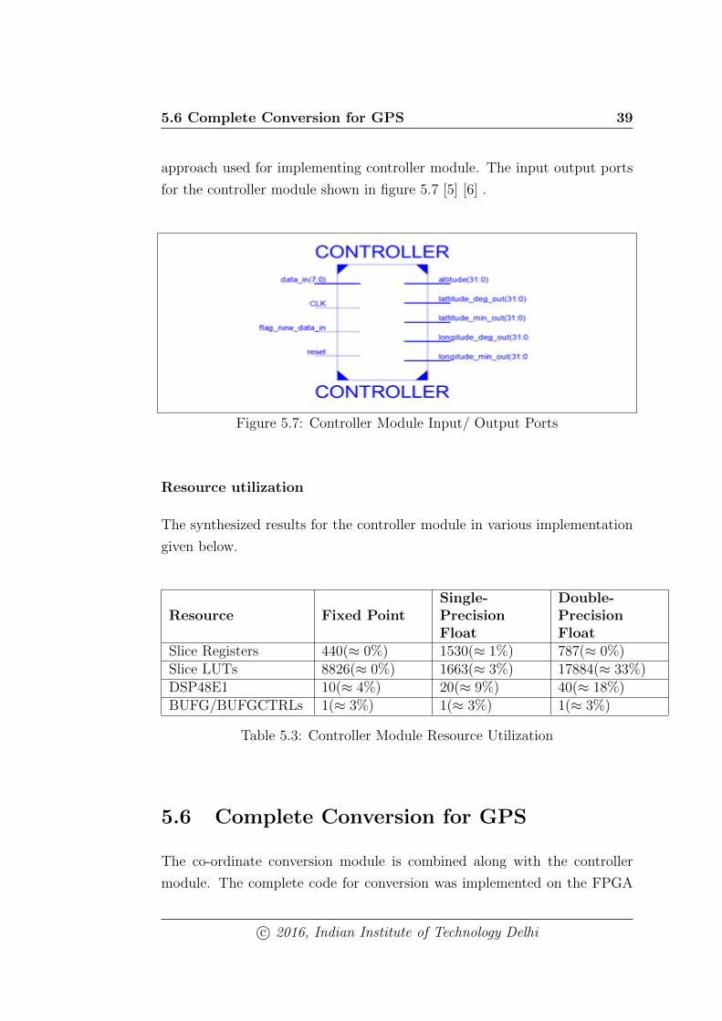
5.6 Complete Conversion for GPS 39
approach used for implementing controller module. The input output ports
for the controller module shown in figure 5.7 [5] [6] .
Figure 5.7: Controller Module Input/ Output Ports
Resource utilization
The synthesized results for the controller module in various implementation
given below.
Resource Fixed PointSingle-PrecisionFloat
Double-PrecisionFloat
Slice Registers 440(≈ 0%) 1530(≈ 1%) 787(≈ 0%)Slice LUTs 8826(≈ 0%) 1663(≈ 3%) 17884(≈ 33%)DSP48E1 10(≈ 4%) 20(≈ 9%) 40(≈ 18%)BUFG/BUFGCTRLs 1(≈ 3%) 1(≈ 3%) 1(≈ 3%)
Table 5.3: Controller Module Resource Utilization
5.6 Complete Conversion for GPS
The co-ordinate conversion module is combined along with the controller
module. The complete code for conversion was implemented on the FPGA
c© 2016, Indian Institute of Technology Delhi
5.6 Complete Conversion for GPS 40
using Xilinx ISE tool. The resource utilization of place and routed imple-
mentation given below.
Resource utilization
The synthesized results for the Complete Conversion for GPS module in var-
ious implementation given below.
Resource Fixed PointSingle-PrecisionFloat
Double-PrecisionFloat
Slice Registers 20684(≈ 19%) 15228(≈ 14%) 17241(≈ 16%)Slice LUTs 21731(≈ 40%) 28073(≈ 52%) 44442(≈ 83%)DSP48E1 98(≈ 44%) 52(≈ 23%) 236 (≈ 107%)BUFG/BUFGCTRLs 1(≈ 3%) 1(≈ 3%) 1(≈ 3%)
Table 5.4: Complete Conversion for GPS Resource Utilization
As we can notice from the results that double precision floating point imple-
mentation was failing to meet the resources. The double precision floating
point design cannot implemented on Zynq FPGA. The other designs were
implemented on Zynq FPGA.
5.6.1 Debug using Chip scope Pro
After configuring the FPGA, the design can be debugged using Chipscope
Pro software. The Chipscope software is performs in-circuit verification of
the design. There are three steps to be followed for debugging the design [3].
• Insert the Chipscope pro into the design using the core inserter tool
• Implement the design and configure the FPGA
• Analyze the design using the Chipscope Pro Analyzer
c© 2016, Indian Institute of Technology Delhi
5.7 Data Capture module for IMU 41
The Complete co-ordinate conversion was verified using the Chipscope Pro
tool.
5.6.2 Vivado-SDK implementation
The custom IP core was created for the complete conversion for GPS. This IP
was imported to Vivado [29] to interface with processor of Zynq. The GPS
IP was interfaced to the ARM using GPIOs. The design was implemented
on FPGA.
Resource Fixed PointSingle-PrecisionFloat
Slice Registers 26886(≈ 25%) 22793(≈ 22%)Slice LUTs 24525(≈ 46%) 27587(≈ 52%)DSP48E1 82(≈ 37.27%) 44(≈ 19%)BUFG/BUFGCTRLs 1(≈ 3%) 1(≈ 3%)
Table 5.5: Complete Conversion (Vivado) Resource Utilization
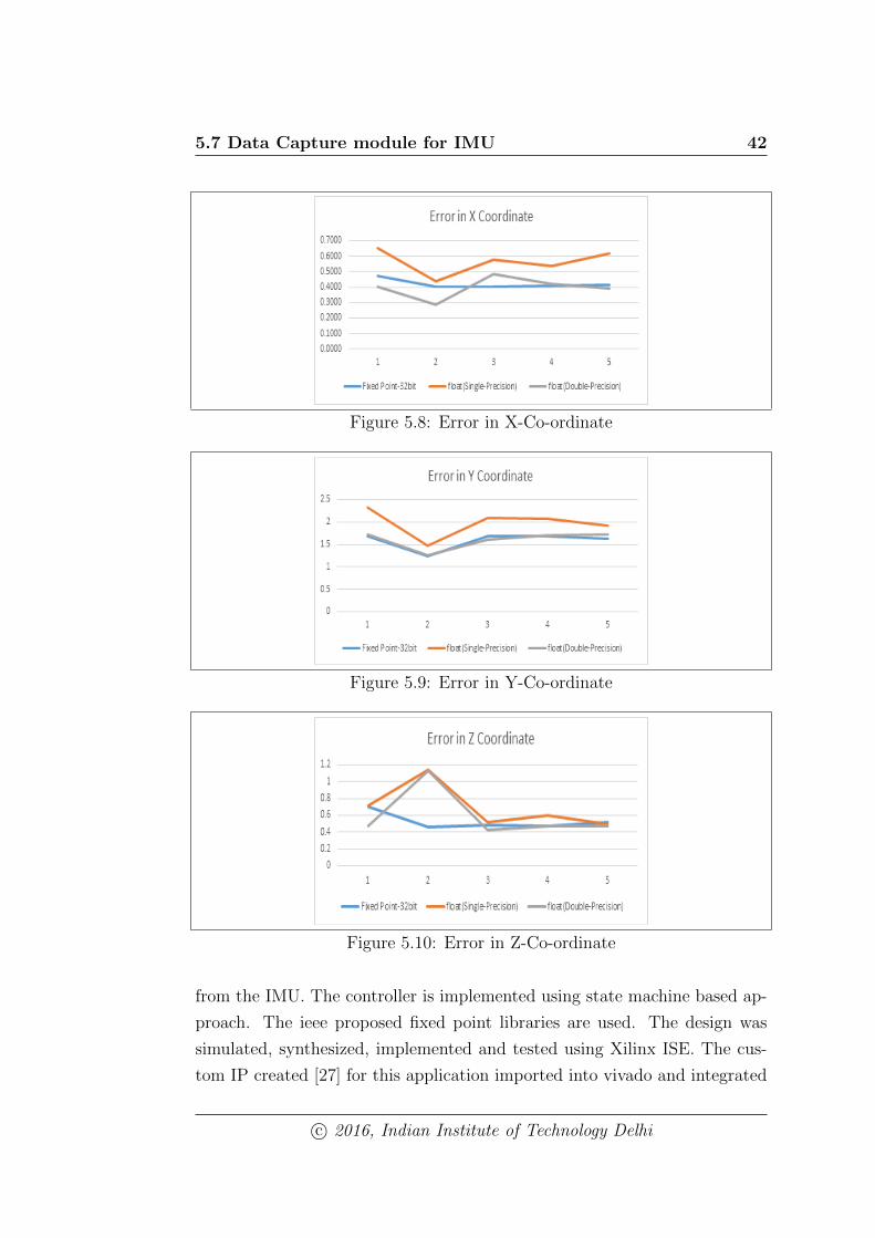
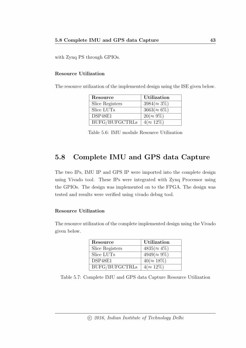
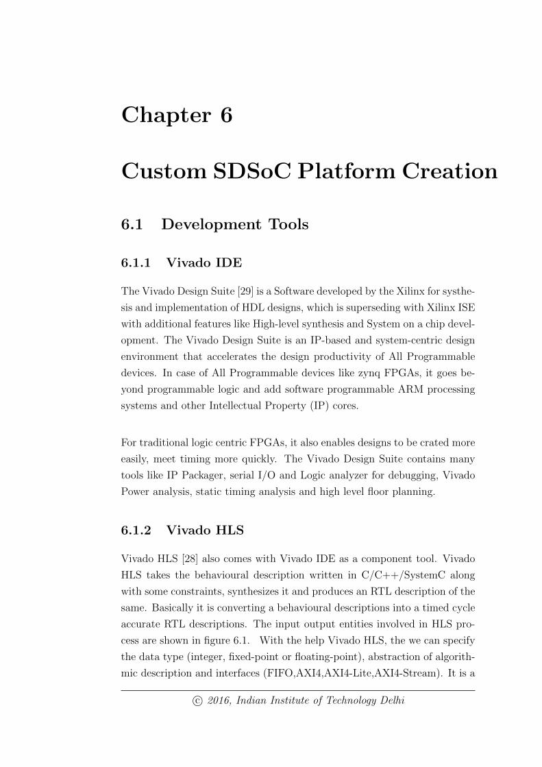
Conversion Error Results
The co-ordinate conversion results were compared with matlab implemented
results and errors were calculated. The GPS co-ordinates are captured and
averaged for 50 readings at 5 different locations. The error plots in three axis
are shown below figures 5.8 5.9 5.10.
5.7 Data Capture module for IMU
The IMU send the acceleration and angular rate velocity data using UART
protocol. The UART module was implemented on FPGA and connected to
IMU through PMOD connector. The data was captured at 57600bps data
rate. The fixed point controller module is implemented to decode the data
c© 2016, Indian Institute of Technology Delhi
5.7 Data Capture module for IMU 42
Figure 5.8: Error in X-Co-ordinate
Figure 5.9: Error in Y-Co-ordinate
Figure 5.10: Error in Z-Co-ordinate
from the IMU. The controller is implemented using state machine based ap-
proach. The ieee proposed fixed point libraries are used. The design was
simulated, synthesized, implemented and tested using Xilinx ISE. The cus-
tom IP created [27] for this application imported into vivado and integrated
c© 2016, Indian Institute of Technology Delhi
5.8 Complete IMU and GPS data Capture 43
with Zynq PS through GPIOs.
Resource Utilization
The resource utilization of the implemented design using the ISE given below.
Resource UtilizationSlice Registers 3984(≈ 3%)Slice LUTs 3663(≈ 6%)DSP48E1 20(≈ 9%)BUFG/BUFGCTRLs 4(≈ 12%)
Table 5.6: IMU module Resource Utilization
5.8 Complete IMU and GPS data Capture
The two IPs, IMU IP and GPS IP were imported into the complete design
using Vivado tool. These IPs were integrated with Zynq Processor using
the GPIOs. The design was implemented on to the FPGA. The design was
tested and results were verified using vivado debug tool.
Resource Utilization
The resource utilization of the complete implemented design using the Vivado
given below.
Resource UtilizationSlice Registers 4835(≈ 4%)Slice LUTs 4949(≈ 9%)DSP48E1 40(≈ 18%)BUFG/BUFGCTRLs 4(≈ 12%)
Table 5.7: Complete IMU and GPS data Capture Resource Utilization
c© 2016, Indian Institute of Technology Delhi
Chapter 6
Custom SDSoC Platform Creation
6.1 Development Tools
6.1.1 Vivado IDE
The Vivado Design Suite [29] is a Software developed by the Xilinx for systhe-
sis and implementation of HDL designs, which is superseding with Xilinx ISE
with additional features like High-level synthesis and System on a chip devel-
opment. The Vivado Design Suite is an IP-based and system-centric design
environment that accelerates the design productivity of All Programmable
devices. In case of All Programmable devices like zynq FPGAs, it goes be-
yond programmable logic and add software programmable ARM processing
systems and other Intellectual Property (IP) cores.
For traditional logic centric FPGAs, it also enables designs to be crated more
easily, meet timing more quickly. The Vivado Design Suite contains many
tools like IP Packager, serial I/O and Logic analyzer for debugging, Vivado
Power analysis, static timing analysis and high level floor planning.
6.1.2 Vivado HLS
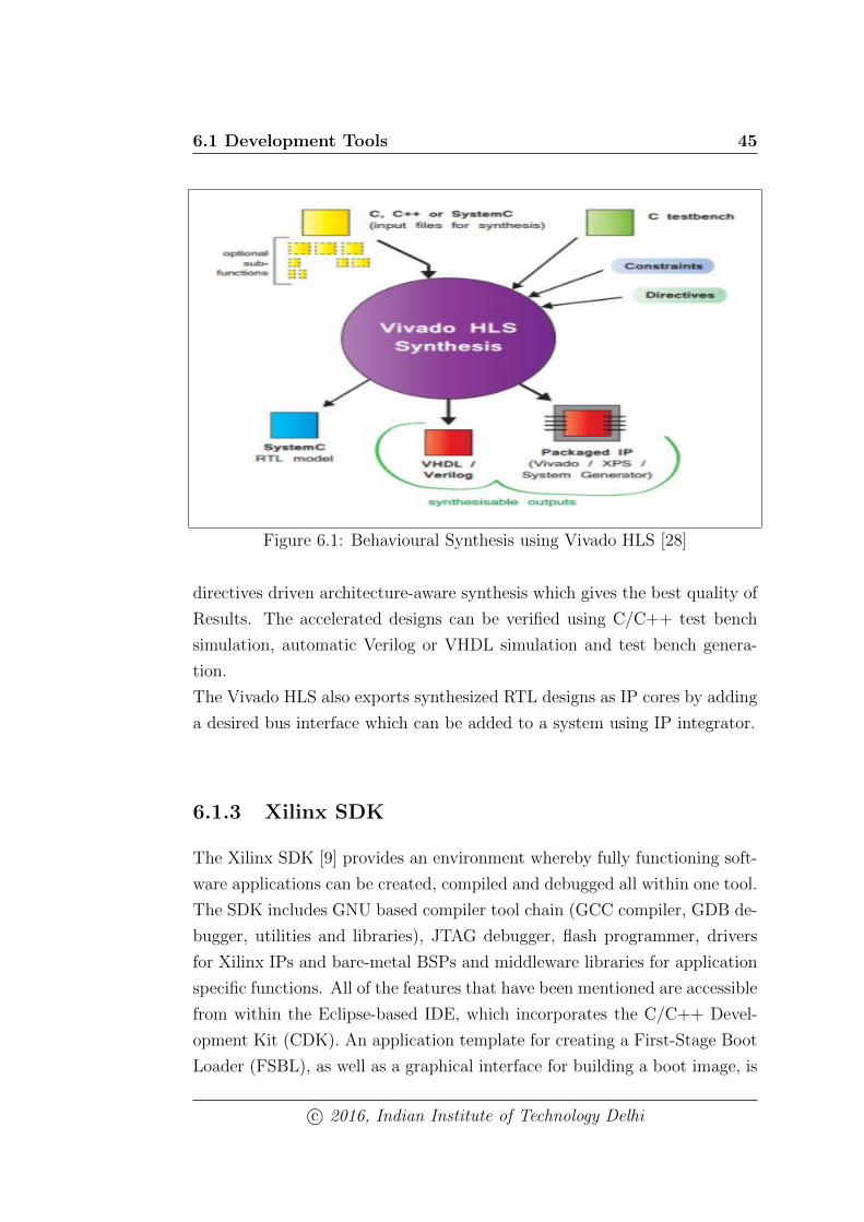
Vivado HLS [28] also comes with Vivado IDE as a component tool. Vivado
HLS takes the behavioural description written in C/C++/SystemC along
with some constraints, synthesizes it and produces an RTL description of the
same. Basically it is converting a behavioural descriptions into a timed cycle
accurate RTL descriptions. The input output entities involved in HLS pro-
cess are shown in figure 6.1. With the help Vivado HLS, the we can specify
the data type (integer, fixed-point or floating-point), abstraction of algorith-
mic description and interfaces (FIFO,AXI4,AXI4-Lite,AXI4-Stream). It is a
c© 2016, Indian Institute of Technology Delhi
6.1 Development Tools 45
Figure 6.1: Behavioural Synthesis using Vivado HLS [28]
directives driven architecture-aware synthesis which gives the best quality of
Results. The accelerated designs can be verified using C/C++ test bench
simulation, automatic Verilog or VHDL simulation and test bench genera-
tion.
The Vivado HLS also exports synthesized RTL designs as IP cores by adding
a desired bus interface which can be added to a system using IP integrator.
6.1.3 Xilinx SDK
The Xilinx SDK [9] provides an environment whereby fully functioning soft-
ware applications can be created, compiled and debugged all within one tool.
The SDK includes GNU based compiler tool chain (GCC compiler, GDB de-
bugger, utilities and libraries), JTAG debugger, flash programmer, drivers
for Xilinx IPs and bare-metal BSPs and middleware libraries for application
specific functions. All of the features that have been mentioned are accessible
from within the Eclipse-based IDE, which incorporates the C/C++ Devel-
opment Kit (CDK). An application template for creating a First-Stage Boot
Loader (FSBL), as well as a graphical interface for building a boot image, is
c© 2016, Indian Institute of Technology Delhi
6.1 Development Tools 46
also included in the SDK. Xilinx SDK is used to develop the software appli-
cation for the system.
6.1.4 Xilinx SDSoC
The SDSoC [10] (software defined system-on-chip) development environment
provides an embedded C/C++ application development experience for Zynq
All Programmable SoC. It has complete industrys first C/C++ full system
optiminzing compiler, System level Profiler, automated software acceleration
in programmable logic and automated system connectivity generation. It
supports bare metal, Linux and FreeRTOS as target OS.
The SDSoC system compilers analyze a program to determine the data flow
between software and hardware functions, and generate an application spe-
cific system on chip. We can achieve high performance by configuring each
hardware function runs as an independent thread. The system compilers
ensures synchronization between hardware and software threads and enables
pipelined computation. The SDSoC system compilers can invoke the Vivado
HLS tool to compile the synthesizable C/C++ functions into programmable
logic. The tool generate a complete hardware system which includes DMAs,
interconnects, hardware buffer and other IPs, and it also configures the
FPGA by invoking the Vivado tools.
SDSoC (Software Defined System-on-Chip) is a C/C++ environment for
complete embedded system design on heterogeneous platform of Zynq us-
ing hardware/software partitioning. SDSoC performs program analysis, task
scheduling and binding onto processor and configurable logic for accelerator,
specified by user. SDSoC compiler and linker generates code for hardware
and software that automatically orchestrates communication and cooperation
among hardware and software components . User can play around with dif-
ferent accelerators by just toggling the target of that function, i.e. hardware
or software. It invokes Vivado HLS for accelerator and interface synthesis,
then makes connections in Vivado Design Suite and generates the bitfile.
Thereafter it generates object code for processor using GNU toolchain. It
also generates the bootfiles: kernel image, devicetree, boot-image etc. to
c© 2016, Indian Institute of Technology Delhi
6.1 Development Tools 47
run the application from ramdisk. User can optimize the hardware by using
pragmas and he/she can also decide a datamover type and PS-port which
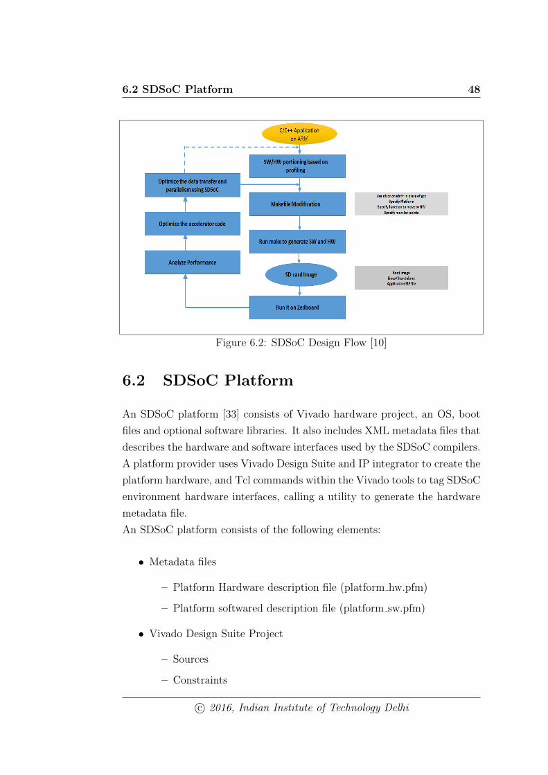
will be interfaced to accelerator. In the Figure 6.2 , the design flow is clearly
depicted. The some important points are:
• User will profile the code and will define the hotspot function as HW
target. More than one accelerator is also possible here.
• The hardware is synthesized using Vivado HLS and so HLS guidelines
should be followed. HLS pragmas or compiler directives can be used to
optimize the hardware.
• The code is compiled by sdscc for C-code, sds++ for C++ code.
• The SDSoC linker creates SD card image to implement the application
in Linux environment.
• SDSoC also gives provision to decide specific data-movers: AXI DMA
in simple mode, AXI DMA scatter-gather mode etc and PS-PL inter-
face ports: ACP, HP, GP etc by using pragmas.
• In Linux, memory allocation is done in virtual space always. It is dis-
tributed across multiple pages in physical space. DMA or any hardware
operates on physical address only. So for each memory allocation, the
elements must be mapped to physical space. Scatter-gather DMA can
handle such list of pages, whereas simple DMA can handle only single
page [32].
• SDSoC provides mechanism to allocate contiguous memory in physical
address space using sds alloc and sds free. Basically Linux kernel also
has support for CMA (contiguous memory allocator).
• So in Linux, memory allocated by malloc can be taken care of by
scatter-gather DMA, where as simple DMA handles memory allocated
by sds alloc
c© 2016, Indian Institute of Technology Delhi
6.2 SDSoC Platform 48
Figure 6.2: SDSoC Design Flow [10]
6.2 SDSoC Platform
An SDSoC platform [33] consists of Vivado hardware project, an OS, boot
files and optional software libraries. It also includes XML metadata files that
describes the hardware and software interfaces used by the SDSoC compilers.
A platform provider uses Vivado Design Suite and IP integrator to create the
platform hardware, and Tcl commands within the Vivado tools to tag SDSoC
environment hardware interfaces, calling a utility to generate the hardware
metadata file.
An SDSoC platform consists of the following elements:
• Metadata files
– Platform Hardware description file (platform hw.pfm)
– Platform softwared description file (platform sw.pfm)
• Vivado Design Suite Project
– Sources
– Constraints
c© 2016, Indian Institute of Technology Delhi

6.2 SDSoC Platform 49
– IP blocks
• Software files
– Library header files (optional)
– Static kibraries (optional)
– Linux related objects (device-tree, U-boot, Linux-kernel, ramdisk)
• Pre-built hardware files (optinal)
– Bitstream
– Exported hardware files for SDK
– Pregenerated hardware and software interface files
– Pre-generated device registration and port information software
files
Figure 6.3: Directory Structure for a Typical SDSoC Platform [10]
6.2.1 Steps to Generate SDSoc Hardware Platform De-
scription
• Create the hardware design using vivado design suite.
c© 2016, Indian Institute of Technology Delhi
6.2 SDSoC Platform 50
• Run the following command in the Vivado Tcl console to enable SD-
SoC platform hardware description generation
set param project.enablePlatformHandoff true
• Next declare the default platform clock by following command
set property SDSOC PFM.PFM CLOCK TRUE [get bd pins /ps7/FCLK CLK2]
• Next declare the platform clocks and their IDs
set property SDSOC PFM.CLOCK ID2 [get bd pins/ps7/FCLK CLK2]
set property SDSOC PFM.MARK SDSOC true [get bd pins/ps7/FCLK CLK2]
• Next step is to synchronize the platform resets to specific clock using
proc sys reset IP blocks
set property SDSOC PFM.MARK SDSOC true
[get bd pins/proc sys reset 2/interconnect aresetn]
set property SDSOC PFM.MARK SDSOC true
[get bd pins/proc sys reset2/peripheral aresetn]
set property SDSOC PFM.MARK SDSOC true
[get bd pins/proc sysreset 2/peripheral reset]
• Next declare the axi gpio IP block as a UIO device. To support linux
applications, the platform provides a userspace library to write or read
to the I/O s on the Linux UIO framework.
set property SDSOC PFM.UIO true [get bd cells/axi gpio ∗]
• Now generate the bitstream , after the bitstream generation export the
hardware description and do not select the include the bitstream as
part of the handoff.
• Next step open the Tcl console of SDSoC and invoke the HSI utility
and following commands to generate the SDSoC platform description.
c© 2016, Indian Institute of Technology Delhi
6.2 SDSoC Platform 51
load features hsi
hsi::open hw design project name.sdk/project name wrapper.hdf
hsi::generate target sdsoc [hsi::current hw design] dir ..
This step generate the hardware platform description file in the parent
directory, which will support Linux and standalone applications.
• Exit the Vivado and remove unnecessary project directories by running
following commands
rm -rf zc702 acp.cache
rm -rf zc702 led.hw
rm -rf zc702 led.runs
rm -rf zc702 led.sdk
rm -rf zc702 led.sim
rm -rf vivado
• In case 2015.2 release version, the project name hw.pfm needs to be
modified. Open in a text editor to make following changes.
Replace the device capacity attributes in xd:component for the xc7z020
device as follows.
<xd:component xd:BRAM=140 xd:DSP=220 xd:FF=106400 xd:LUT=53200
Replace the platform resource usage attributes in xd:resourceEstimates
as follows
<xd:resourceEstimates xd:BRAM=-1 xd:DSP=-1 xd:FF=-1 xd:LUT=-
1 />
Where -1 indicates uncomputed
Validate the hardware description file using the SDSoC terminal shell.
sds-pf-check ../project name hw.pfm
6.2.2 Steps to generate SDSoC Software Plaform De-
scription
The SDSoC platform software description is an XML file that contain re-
quired to link against platform libraries and create boot images to run the
c© 2016, Indian Institute of Technology Delhi
6.2 SDSoC Platform 52
application on the hardware platform
• Open the software platform description project name sw.pfm
The following element instructs the SDSoC environment where to find
the platform software libraries created in the platform directory.
<xd:libraryFiles
xd:os=”linux”
xd:includeDir=”arm-xilinx-linux-gnueabi/include”
xd:libDir=”arm-xilinx-linux-gnueabi/lib”
xd:libName=zc702 axis io
/>
• Similarly, the boot files are specified as follows:
<xd:bootFiles xd:os=”linux”
xd:bif=”boot/linux.bif”
xd:readme=boot/generic.readme
xd:devicetree=”boot/devicetree.dtb”
xd:linuxImage=”boot/uImage”
xd:ramdisk=”boot/uramdisk.image.gz”
/>
The GPIOs can be included to the Linux Software Plaform, by updat-
ing the Linux device tree. The device tree is to be manually created by
modifying the devicetree.dtb from the platform. The devicetree.dtb is
first converted into text format using the dtc compiler.
dtc -I dtb -O dts -o devicetree.dts boot/devicetree.dtb
There are two changes are required to the device tree file devicetree.dts, to
register the axi gpios platform peripherals with the Linux.
c© 2016, Indian Institute of Technology Delhi
6.2 SDSoC Platform 53
• First Add uio pdrv genirq.of id=generic-uio to bootargs as follows
bootargs=console=ttyPSO, 115200 root=/dev/ram rw earlyprintk uio pdrv genirq.of
=generic-uio;
• Next add the device tree blob to it for all gpios, check gpio address
from the Vivado address editor.
gpio@41200000 compatible = ”generic-uio”;
reg = <0x41200000 0x10000>;
;
• Next step is to convert back the device tree to binary format required
by the Linux kernel.
dtc -I dts -O dtb -o devicetree.dtb boot/devicetree.dts
c© 2016, Indian Institute of Technology Delhi
Chapter 7
Software Implementation and Ac-
celeration Using Vivado-HLS
In order to communicate with the hardware and get the programmable func-
tionality software programming is required. In order to interface with hard-
ware the Xilinx provided Software Development Kit (SDK) and SDSoC. The
Xilinx SDK provides an environment whereby fully functioning software ap-
plications can be created, compiled and debugged all within one tool.
7.1 Functions implemented in SDK
7.1.1 IEEE-74 Single Point to Hex Conversion
The Single Precision floating point data required to send to the Hardware,
where the actual co-ordinate conversion taking place. The float data is rep-
resented in 32 bit hex format as referred in the figure 5.5 . The conversion
was implemented in software [8].
7.1.2 Hex to IEEE-754 Single Point Float Conversion
Hex to IEEE-754 floating point conversion is required in order to display the
data on the terminal. The GPS latitude, longitude and altitude co-ordinates
are converted into X, Y and Z co-ordinates. These co-ordinates were out-
putted on the terminal. The conversion algorithm was implemented using
SDK software. The 32 bit hex data was converted into float values.
c© 2016, Indian Institute of Technology Delhi
7.2 SDSoC implementation 55
7.1.3 Fixed Point to Hex Conversion
The 32 bit fixed point data is used in the conversion algorithms. The data
received from the UART will be converted into the 32 bit Hex value [6].
7.1.4 Hex to Fixed Point Conversion
Hex to Fixed Point conversion is required in order to display the data on
the terminal. The GPS latitude, longitude and altitude co-ordinates are
converted into X, Y and Z co-ordinates. These co-ordinates were outputted
on the terminal.
7.2 SDSoC implementation
The Localization algorithm was implemented in SDSoC. The data sampling
of Sensors GPS and IMU was implemented in the hardware. The GPS pro-
vides the co-ordinates (latitude, longitude, altitude) and IMU provides the
acceleration in 3 axis, angular rates in 3 axis and Euler angles. This in-
formation was passed to the Processor (Processing System) with the help of
GPIOs .There are multiple GPIOs which are interfaced to Zynq PS. There are
three modules in SDSoC implementation. i.e, IMU Mechanization, Kalman
filter and Error update module. The fourth order Runga-kutta numerical
integration is used.
7.2.1 IMU Mechanization
The IMU mechanization requires the following data as the input to apply
mechanization equations to calculate the position and velocity of moving
object [20].
• ax,ay, az accelerations of the accelerometers in m/s2
• p, q, r are the roll, pitch and yaw rates from the gyroscopes in radians
per second,
c© 2016, Indian Institute of Technology Delhi
7.3 Accelerator Synthesis using Vivado HLS 56
• φ,θ, ψ are the Euler angles in radians,
• X, Y, Z are the distances along the three axes in the navigation frame
in meters,
• VT ,α,β are the velocity of the aircraft in m/s, the angle of attack in
radians and the sideslip angle in radians, respectively.
The set of equations given in the chapter 3 can be applied to calculate the
position. For each time the algorithm starts the initial position of current
location should be given to algorithm.
7.2.2 Kalman Filter module
There are four set of equations which is applied interactively to correct the
error occurred in the position calculation.
All the error matrices used are initialized to zero before starting filtering
operation. The matrices Rk and Qdev holds the variance of the GPS, ac-
celerometer and Gyroscope respectively. The 9-state Kalman filter used. The
four equations were implemented using the For-loops. The 3 *3 matrix in-
version was implemented. The Kalman filter algorithm was applied at every
0.5sec to correct the errors.
7.3 Accelerator Synthesis using Vivado HLS
This section deals with behavioural synthesis of the hotspots identified after
partitioning by profiling the application. With the help of SDSoC [10] the
hotspot function can be mapped to Hardware. The clock period and the
implementation platform needs to be specified while converting an untimed
description to a timed description. The synthesis process can be tuned to
improve the performance and reduce resources by applying directives. Direc-
tives are applied at various levels, i.e.., function level, block level and loop
c© 2016, Indian Institute of Technology Delhi
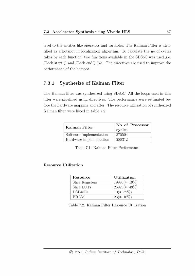
7.3 Accelerator Synthesis using Vivado HLS 57
level to the entities like operators and variables. The Kalman Filter is iden-
tified as a hotspot in localization algorithm. To calculate the no of cycles
takes by each function, two functions available in the SDSoC was used.,i.e.
Clock start () and Clock end() [32]. The directives are used to improve the
performance of the hotspot.
7.3.1 Synthesize of Kalman Filter
The Kalman filter was synthesized using SDSoC. All the loops used in this
filter were pipelined using directives. The performance were estimated be-
fore the hardware mapping and after. The resource utilization of synthesized
Kalman filter were listed in table 7.2.
Kalman FilterNo of Processorcycles
Software Implementation 375504Hardware implementation 288312
Table 7.1: Kalman Filter Performance
Resource Utilization
Resource UtillizationSlice Registers 19995(≈ 19%)Slice LUTs 25925(≈ 49%)DSP48E1 70(≈ 32%)BRAM 23(≈ 16%)
Table 7.2: Kalman Filter Resource Utilization
c© 2016, Indian Institute of Technology Delhi
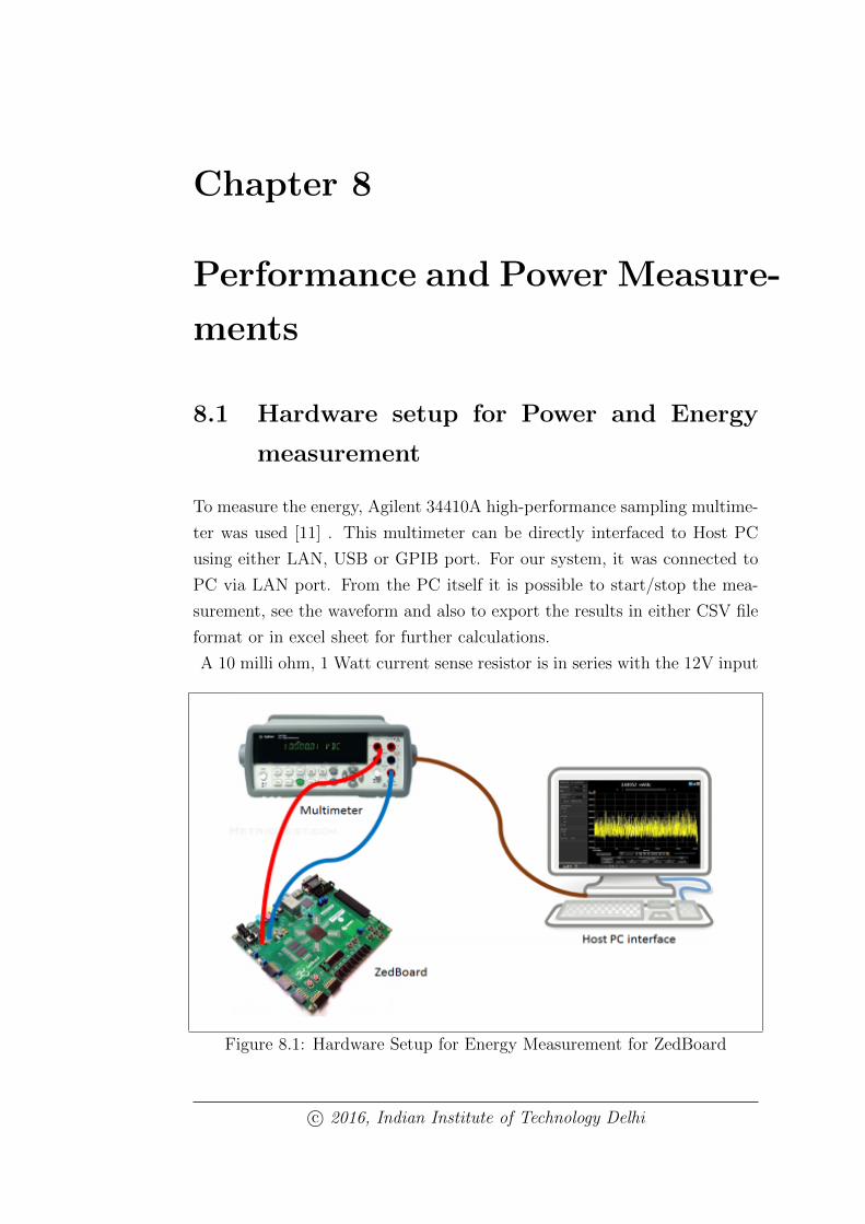
Chapter 8
Performance and Power Measure-
ments
8.1 Hardware setup for Power and Energy
measurement
To measure the energy, Agilent 34410A high-performance sampling multime-
ter was used [11] . This multimeter can be directly interfaced to Host PC
using either LAN, USB or GPIB port. For our system, it was connected to
PC via LAN port. From the PC itself it is possible to start/stop the mea-
surement, see the waveform and also to export the results in either CSV file
format or in excel sheet for further calculations.
A 10 milli ohm, 1 Watt current sense resistor is in series with the 12V input
Figure 8.1: Hardware Setup for Energy Measurement for ZedBoard
c© 2016, Indian Institute of Technology Delhi
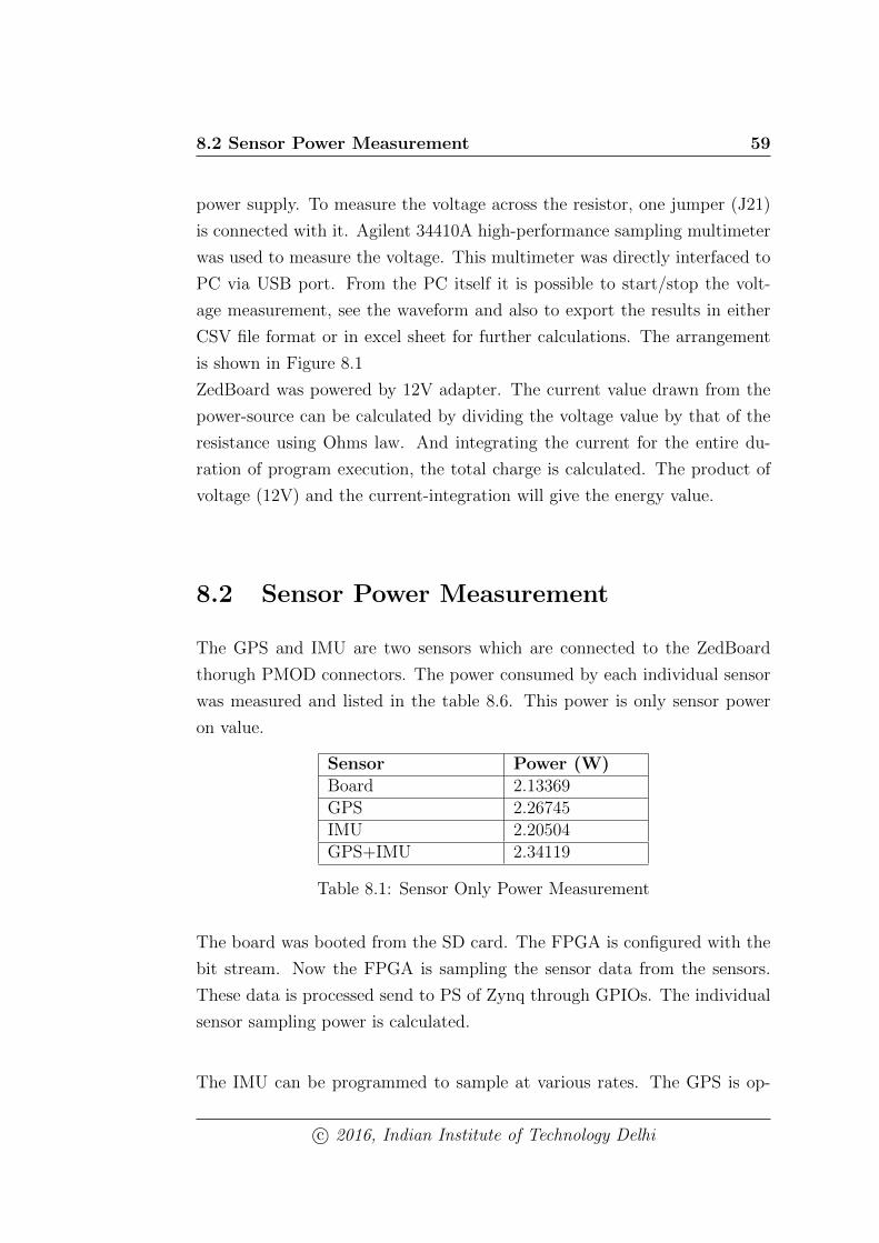
8.2 Sensor Power Measurement 59
power supply. To measure the voltage across the resistor, one jumper (J21)
is connected with it. Agilent 34410A high-performance sampling multimeter
was used to measure the voltage. This multimeter was directly interfaced to
PC via USB port. From the PC itself it is possible to start/stop the volt-
age measurement, see the waveform and also to export the results in either
CSV file format or in excel sheet for further calculations. The arrangement
is shown in Figure 8.1
ZedBoard was powered by 12V adapter. The current value drawn from the
power-source can be calculated by dividing the voltage value by that of the
resistance using Ohms law. And integrating the current for the entire du-
ration of program execution, the total charge is calculated. The product of
voltage (12V) and the current-integration will give the energy value.
8.2 Sensor Power Measurement
The GPS and IMU are two sensors which are connected to the ZedBoard
thorugh PMOD connectors. The power consumed by each individual sensor
was measured and listed in the table 8.6. This power is only sensor power
on value.
Sensor Power (W)Board 2.13369GPS 2.26745IMU 2.20504GPS+IMU 2.34119
Table 8.1: Sensor Only Power Measurement
The board was booted from the SD card. The FPGA is configured with the
bit stream. Now the FPGA is sampling the sensor data from the sensors.
These data is processed send to PS of Zynq through GPIOs. The individual
sensor sampling power is calculated.
The IMU can be programmed to sample at various rates. The GPS is op-
c© 2016, Indian Institute of Technology Delhi
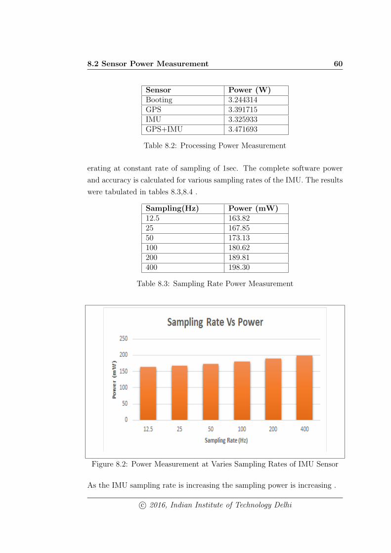
8.2 Sensor Power Measurement 60
Sensor Power (W)Booting 3.244314GPS 3.391715IMU 3.325933GPS+IMU 3.471693
Table 8.2: Processing Power Measurement
erating at constant rate of sampling of 1sec. The complete software power
and accuracy is calculated for various sampling rates of the IMU. The results
were tabulated in tables 8.3,8.4 .
Sampling(Hz) Power (mW)12.5 163.8225 167.8550 173.13100 180.62200 189.81400 198.30
Table 8.3: Sampling Rate Power Measurement
Figure 8.2: Power Measurement at Varies Sampling Rates of IMU Sensor
As the IMU sampling rate is increasing the sampling power is increasing .
c© 2016, Indian Institute of Technology Delhi

8.2 Sensor Power Measurement 61
Sampling(Hz)Accuracy X(m)
Accuracy Y(m)
12.5 11.5 15.725 8.6 11.150 5.9 7.6100 4.1 5.7200 3.4 4.3400 0 0
Table 8.4: Accuracy Measurement at Various Sampling Rates of IMU Sensor
Figure 8.3: Accuracy Measurement at Various Sampling Rates of IMU Sensor
Kalman Filter is partitioned to be hardware. The power was calculated for
software and Hardware for the case of Kalman Filter. In this case the IMU
is sampled at constant rate of 100Hz.
The IMU can be programmed to sample at various rates. The GPS is
operating at constant rate of sampling of 1sec. The engergy taken for each
case is calculated. The results were tabulated in tables .The localization
is a dedicated module which required to operate all the time. The time
required for algorithm to calculate the position is ’t’ and the remaining time
this module is ideal. Presently this module is independently working so the
processor time is not effectively used for other purposes.When the module is
c© 2016, Indian Institute of Technology Delhi
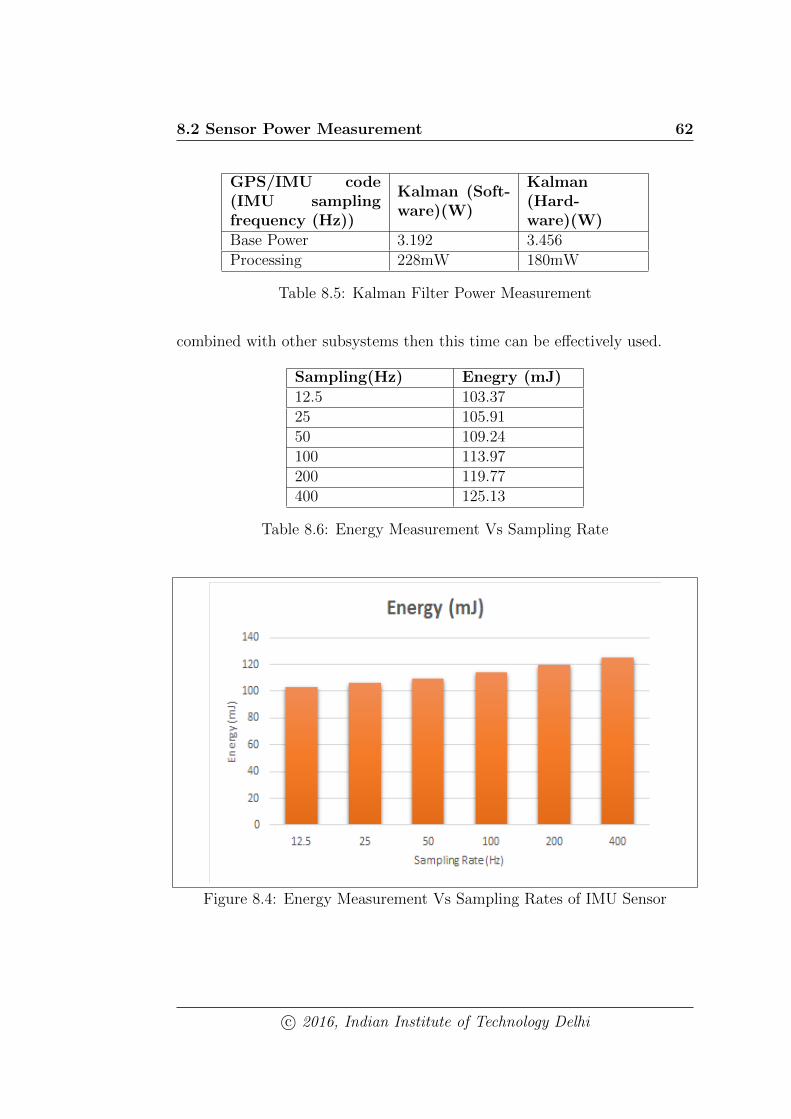
8.2 Sensor Power Measurement 62
GPS/IMU code(IMU samplingfrequency (Hz))
Kalman (Soft-ware)(W)
Kalman(Hard-ware)(W)
Base Power 3.192 3.456Processing 228mW 180mW
Table 8.5: Kalman Filter Power Measurement
combined with other subsystems then this time can be effectively used.
Sampling(Hz) Enegry (mJ)12.5 103.3725 105.9150 109.24100 113.97200 119.77400 125.13
Table 8.6: Energy Measurement Vs Sampling Rate
Figure 8.4: Energy Measurement Vs Sampling Rates of IMU Sensor
c© 2016, Indian Institute of Technology Delhi
Chapter 9
Conclusion and Future Work
This thesis has presented loosely coupled localization using GPS/IMU in-
tegration. The IMU sensor and GPS Sensors were interfaced to ZedBoard
through PMOD connectors. The data from GPS and IMU sensors are sam-
pled at 9600bps and 57600bps using the UART protocol. The Custom
Generic UART was implemented to sample the data from the sensors. The
Zynq PL side the data sampling was implemented using RTL. The custom
SDSoC platform was created which holds the hardware interfaces with GPS
and IMU on PL side. The IMU mechanization and Kalman Filter were im-
plemented in PS side of Zynq. The hotspot identified as Kalman Filter which
taking more no of processor cycles of Processor. The Kalman Filter was syn-
thesized using Vivado HLS mapped to Hardware. The accuracy, power and
energy were calculated for various sampling rates of IMU. With the help of
Zed board the localization was implemented using Hardware software co-
design.
9.1 Future Work
The accuracy can be further improved if the no of states of the Kalman
filter increased to includes the scale factors and biases of the sensors. The
Accuracy can be further improved by using cameras. The vision algorithm
make it more robust. Integration of IMU, GPS with Vision provides better
estimates of location along with adding redundancy to the system.
c© 2016, Indian Institute of Technology Delhi
Bibliography
[1] 9 degrees of freedom - razor imu. https://www.sparkfun.com/
products/10736. Accessed: 2016-06-16.
[2] Building an ahrs using the sparkfun ”9dof razor imu”. https://github.
com/ptrbrtz/razor-9dof-ahrs/wiki/Tutorial. Accessed: 2016-06-
16.
[3] Chipscope pro debugging. http://www.xilinx.com/itp/xilinx10/
isehelp/ise_c_process_analyze_design_using_chipscope.htm.
Accessed: 2016-06-16.
[4] Double-precision floating-point format. https://en.wikipedia.org/
wiki/Double-precision_floating-point_format. Accessed: 2016-
06-16.
[5] Fixed point operations. https://forums.xilinx.com/t5/Synthesis/
ieee-proposed-fixed-pkg-all-in-Xilinx-ISE-12-1/td-p/75873.
Accessed: 2016-06-16.
[6] Fixed point operations. http://vhdlguru.blogspot.in/2010/03/
fixed-point-operations-in-vhdl-tutorial.html. Accessed: 2016-
06-16.
[7] Nmea data. http://www.gpsinformation.org/dale/nmea.htm. Ac-
cessed: 2016-06-16.
[8] Single-precision floating-point format. https://en.wikipedia.org/
wiki/Single-precision_floating-point_format. Accessed: 2016-
06-16.
[9] Xilinx sdk. http://www.xilinx.com/support/documentation/sw_
manuals/xilinx2015_1/SDK_Doc/index.html. Accessed: 2016-06-16.
[10] Xilinx sdsoc. http://www.xilinx.com/products/design-tools/
software-zone/sdsoc.html#training. Accessed: 2016-06-16.
[11] Agilent. Agilent 34410A Digit Multimeter, 1 2007. Rev 1.0.
c© 2016, Indian Institute of Technology Delhi
BIBLIOGRAPHY 65
[12] Analog Devices. ITG-3200 3-Axis Gyro Evaluation Board, 3 2010. Rev.
1.1.
[13] Analog Devices. Digital Accelerometer, 6 2011. Rev. E.
[14] Vishisht Gupta. Vehicle localization using low-accuracy gps, imu and
map-aided vision, 2009. The Pennsylvania State University.
[15] Honeywell. 3-Axis Digital Compass IC, 3 2011. Rev. D.
[16] InvenSense. Register Map and Register Descriptions, 6 2011. Revision
1.0.
[17] Jussi Collin Lucian Ioan Iozan and Jarmo Takala. Integrating mems sen-
sors with gps technology for obtaining a continuous navigation solution
in urban areas, 2011. Technical University of Cluj-Napoca.
[18] Scott M. Martin. Closely coupled gps/ins relative positioning for auto-
mated vehicle convoys, 2011. Auburn University.
[19] Lawrence R.Weill Mohinder S.Grewal and Angus P.Andrews. Global
positioning systems, inertial navigation, and integration, 2001.
[20] Vikas Kumar N. The new reno modification to tcp’s fast recovery algo-
rithm, 2004. INDIAN INSTITUTE OF TECHNOLOGY, BOMBAY.
[21] TOBIAS ODENMAN NIKLAS MAGNUSSON. Improving absolute po-
sition estimates of an automotive vehicle using gps in sensor fusion, 2002.
CHALMERS UNIVERSITY OF TECHNOLOGY.
[22] Ahmed Abdulla Ameer Yousef Othman Maklouf, Abdurazag Ghila. Low
cost imu gps integration using kalman filtering for land vehicle naviga-
tion application, 2013. International Journal of Electrical, Computer,
Energetic, Electronic and Communication Engineering.
[23] Eun-Hwan Shin. Accuracy improvement of low cost ins/gps for land
applications, 2001. University of Calgary.
[24] Eun-Hwan Shin. Estimation techniques for low-cost inertial navigation,
2005. University of Calgary.
c© 2016, Indian Institute of Technology Delhi
BIBLIOGRAPHY 66
[25] SIM Com. SIM28 Hardware Design, 5 2013. V1.06.
[26] SIM Com. SIM28 Specification, 5 2013. Rev 1242.
[27] Xilinx. Creating and Packaging Custom IP, 10 2014. v2014.3.
[28] Xilinx. High-Level Synthesis, 10 2014. v2014.3.
[29] Xilinx. Vivado Design Suite User Guide, 4 2014. v2014.1.
[30] Xilinx. The Zynq Book, 5 2014. Rev 0.
[31] Xilinx. Model-Based DSP Design Using System Generator, 9 2015.
v2015.3.
[32] Xilinx. SDSoC Environment User Guide, 9 2015. Rev. 2.
[33] Xilinx. ug1146-sdsoc-platforms-and-libraries, 9 2015. Rev. 2.
[34] Yueming Zhao. Gps/imu integrated system for land vehicle navigation
based on mems, 2011. Royal Institute of Technology.
c© 2016, Indian Institute of Technology Delhi