locally owned: do local business ownership and size matter
TRANSCRIPT

Community and Economic Development Discussion Paper No. 01-13 • August 2013
Federal Reserve Bank of Atlanta Community and Economic Development Department 1000 Peachtree Street, N.E. Atlanta, GA 30309-4470
Locally Owned: Do Local Business Ownership and Size
Matter for Local Economic Well-being?
Anil Rupasingha, PhD
Federal Reserve Bank of Atlanta
Community and Economic Development Department

1
The Federal Reserve Bank of Atlanta’s Community and Economic
Development Discussion Paper Series addresses emerging and critical issues in
community development. Our goal is to provide information on topics that will be
useful to the many actors involved in community development—governments,
nonprofits, financial institutions, and beneficiaries. frbatlanta.org/commdev/
No. 01-13 • August 2013
Locally Owned: Do Local Business Ownership and Size
Matter for Local Economic Well-being?
Abstract: The concept of “economic gardening”—supporting locally owned businesses over nonlocally owned businesses and small businesses over large ones—has gained traction as a means of economic development since the 1980s. However, there is no definitive evidence for or against this pro-local business view. Therefore, I am using a rich U.S. county-level data set to obtain a statistical characterization of the relationship between local-based entrepreneurship and county economic performance for the period 2000–2009. I investigate the importance of the size of locally based businesses relative to all businesses in a county measured by the share of employment by local businesses in total employment. I also disaggregate employment by local businesses based on the establishment size. My results provide evidence that local entrepreneurship matters for local economic performance and smaller local businesses are more important than larger local businesses for local economic performance.
JEL Classification: O18, R11 Key words: local ownership, small business, firm size, income growth, employment growth, poverty, rural
About the Author: Anil Rupasingha is a research adviser and economist in the community and economic development (CED) group at the Federal Reserve Bank of Atlanta. His major fields of study are microbusiness and small business, entrepreneurship, self-employment, regional income growth and poverty, internal migration, and social capital. Prior to joining the Atlanta Fed in 2011, Rupasingha was a faculty member in the Department of Agricultural Economics at New Mexico State University, and prior to that in the Department of Economics at American University of Sharjah in the United Arab Emirates, a senior research associate in the Northeast Regional Center for Rural Development at Pennsylvania State University, and a postdoctoral fellow in TVA rural studies at the University of Kentucky.
He has published his research in various journals, including American Journal of Agricultural Economics, Annals of Regional Science, Economic Development Quarterly, Journal of Economic Behavior and Organization, Papers in Regional Science, and Review of Agricultural Economics. A native of Sri Lanka, Rupasingha received a BA in economics from the University of Peradeniya (Sri Lanka). He earned his PhD in agricultural economics at Texas A&M University.
Acknowledgments: I am indebted to Chris Cunningham, Michael Fritsch, Stephan Goetz, Todd Greene, Karen Leone de Nie, and Urvi Neelakantan for helpful comments. An earlier version of this paper was presented at the 58th Annual North American Regional Science Association Meetings, held in Miami, Florida, in November 2011. The views expressed here are the author’s and not necessarily those of the Federal Reserve Bank of Atlanta or the Federal Reserve System. Any remaining errors are the author’s responsibility.
Comments to the author are welcome at [email protected].

Federal Reserve Bank of Atlanta Community and Economic Development Discussion Paper Series • No. 01-13
2
Introduction
In most counties in the U.S., the percent of workers employed by locally- or resident-owned businesses
outweigh the percent of workers employed by nonresident-owned businesses. But this number varies
widely among counties (see Figures 1 and 2). For example, the share of employment in resident
businesses varies from 10.7 percent in Loving County, Texas to 87.2 percent in Franklin County, Texas in
2007. The share of employment in nonresident businesses varies from zero percent in 24 counties
across the nation to 85 percent in Tunica County, Mississippi. This spatial variation is ideal for assessing
whether such variation explains the inter-county variation in economic well-being. The objective of this
paper is twofold: (1) to assess if locally-owned businesses improve local economic performance, and (2)
to I investigate whether the size of the locally-owned businesses affects local economic well-being. I
Figure 1. Spatial variation of workers employed by resident businesses, 2007
Source: Author’s calculation using NETS Database, Edward Lowe Foundation

Federal Reserve Bank of Atlanta Community and Economic Development Discussion Paper Series • No. 01-13
3
Figure 2. Spatial variation of workers employed by nonresident businesses, 2007
Source: Author’s calculation using NETS Database, Edward Lowe Foundation
Historically, the most popular local economic development approach was to attract businesses
from outside a particular municipality, state or region, which was commonly known as industrial
recruitment or “smokestack chasing.” State and local policy makers have been giving numerous
incentives including tax subsidies, low-rent land, and job training subsidies to attract existing firms from
elsewhere. This includes relocation of existing plants or expansion of existing firms. These incentive
policies resulted in fierce competition among states to attract various big plants and large employers to
respective states. For example (see Rork, 2005, for more details), General Motors received offers
consisting of tax breaks and cash subsidies from over 35 different states before choosing to locate its
Saturn plant in Tennessee (1985). Toyota received such incentives from over 30 states before settling
one of its plants in Kentucky (1985). Similar competitions took place before BMW settled in South
Carolina and when Alabama successfully lured Mercedes-Benz (1990s).
This economic development strategy of industrial recruitment presents several challenges and
limitations, especially in terms of a local area’s ability to sustain economic activity. One main problem with
industrial recruitment is that policy makers had little influence over if or when the recruited
establishments wanted to leave. A case in point is labor intensive companies such as call centers.1 The
policy of industrial recruitment may also have led to a tax competition between states that led to a “race
1 Call centers are kind of “foot-loose” businesses due to less capital intensive nature and less intensive labor skill requirements. It is easier for them to relocate to an alternative location that offers attractive incentives once the incentive structure in the current location is exhausted.

Federal Reserve Bank of Atlanta Community and Economic Development Discussion Paper Series • No. 01-13
4
to the bottom.”2 Furthermore, local small businesses, or mom-and-pop stores, face stiff competition from
big firms locating in local communities. On a more positive note, as a companion activity to recruiting
particular plants, some states took steps to improve general business climate in their respective states
using different fiscal incentives to create an environment beneficial to all firms in the state.
However, approaches to local economic development have evolved in the recent past and
economic development based on local entrepreneurship is increasingly gaining traction in the research,
policy, and practice spheres. This approach is a subset of the broader concept of sustainable
development and more generally known as “development from below” or “bottom-up development”
(Coffey and Polese, 1984) or more recently as “economic gardening” (Barrios and Barrios, 2004). The
idea is that directing economic development resources to support local businesses over outside
businesses and local small businesses over big businesses will be beneficial for the local community in
number of ways. One concern is that outside corporations will be less environmentally sensitive to local
communities. Outside firms are also subject to global economic outlook and therefore more amenable
to relocation in other areas than local businesses. Also by favoring local businesses, local communities
are more likely to keep the economic and political power within the local community (Barrios and
Barrios, 2004). The development of local entrepreneurship can lead to a diversified economic structure
that will protect the local economy from being overly dependent on one firm or establishment, or one
industry. The result of local entrepreneurship, it may be presumed, is increased trade within the local
economy, greater export of goods and services out of the local economy, and improved quality of life.
The idea of locally-owned business development is especially favorable for economically distressed rural
areas when it is difficult for these communities to attract outside businesses.
Pro-local business supporters also argue that more local businesses enhance healthy
competition due to the fact that most local businesses are smaller scale operations, increase efficiency,
and increase entrepreneurship in local communities. Kolko and Neumark (2010) argue that locally-
owned firms are more likely to internalize the costs of job loss to communities by not relocating and
closing. There may be other considerations such as “…loyalty toward the headquarters’ hometown or a
desire for better public relations in the headquarters’ hometown, perhaps for political reasons” (Kolko
and Neumark, 2010, p. 103). In addition to these, Kolko and Neumark (2010) point out other specific
economic arguments such as small businesses start-up opportunities for local residents, preserving
businesses in downtown and cultural districts, economic multiplier effects by local businesses spending
more in local communities, local innovation and long-term economic stability in localities. To take
advantage of all these benefits, many local, state and federal governments are initiating numerous
policy approaches to promote locally grown businesses. Numerous localities have enacted policies
favoring locally-owned businesses such as implementing restrictions on formula businesses, store size
cap, local purchasing programs, and set asides for local retail (Kolko and Neumark, 2010). But these
arguments are not without criticisms. For example, some argue that businesses coming from outside to
a locality have been around for a while, are more stable, and may bring higher quality jobs compared to
jobs coming from locally-based firms.
There is no definitive evidence for or against the pro-local business view. For example, numerous
papers (discussed below) suggest that local economic performance in general and employment growth in
2 The phrase “race to the bottom” is commonly used in regional studies literature to convey the behavior of states that
compete with one another by lowering taxes and reducing environmental regulations to attract businesses, which often reduces public revenues for infrastructure, education, and healthcare, for example, and strains environmental conditions.
Federal Reserve Bank of Atlanta Community and Economic Development Discussion Paper Series • No. 01-13
5
particular is strongly associated with smaller average establishment size, but little or no evidence exists
whether these small establishments are resident versus nonresident-owned. The objective of this paper is
to provide such evidence using a new data set. Based on aforementioned claims I investigate whether the
relative size of the locally-owned business sector has a positive association with local economic well-being.
To assess this, I examine the relationship between the percent of establishment-level employment and
local economic indicators such as income and employment growth and change in poverty. I also
investigate whether the different sizes of local businesses have different effects on local economic well-
being. There is evidence on how the size of businesses affects local economies, but not based on whether
the businesses are local or non-local. With the exception of Kolko and Neumark (2010) and Fleming and
Goetz (2011), I am not aware of any research that studies directly the relationship between local
businesses and local economic well-being. One main difference between Kolko and Neumark (2010) and
the present study is that while they look at employment within business establishment, I focus on general
employment growth, income growth and change in poverty in a county. By doing this I am able to capture
the positive externalities of local ownership due to multiplier effects. To capture these effects, I rely on
county-level aggregates rather than establishment-level data. Fleming and Goetz (2011) study the effects
of local and nonlocal businesses on county income growth using establishment counts. In this study I use
employment data as opposed to establishment counts and expand the analysis to study the effects on
employment and poverty.
My resident business measure is the share of the employment in resident business
establishments in total employment by all establishments (resident, non-resident, and noncommercial)
in a county. I assess the relationship between the size of the local business sector and the local income
and employment growth and the change in poverty as measured by the per capita real income growth,
the change in full- and part-time employment, and the change in poverty rate, respectively, averaged
over the period 2000 to 2008.3 Next I disaggregate the measures of percent of employment in resident
establishments into different sizes based on the categorization provided by the data developer Edward
Lowe Foundation (youreconomy.org) and examine the relationship between these various categories on
measures of county economic performance.
The rest of the paper is structured as follows. Section 2 provides a summary of related existing
literature. Descriptive evidence on resident and nonresident employment is provided in Section 3.
Section 4 presents methodology and Section 5 presents descriptive statistics and correlations. Section 6
presents my main results. Section 7 concludes the paper.
Existing Literature
The local entrepreneurship approach is not new and dates back to Schumpeter. Schumpeter (1934) saw
the technological innovation introduced by the entrepreneur playing a central role in economic growth
and development. However, there is a dearth of research that speaks directly to the question of how
locally-owned businesses affect local economic performance. Michelacci and Silva (2007) study factors
affecting the local bias in entrepreneurship (LBE), measured as a fraction of entrepreneurs working in
the region where they were born, including the effects of local unemployment rate and per capita Gross
Domestic Product (GDP). Utilizing data from the United States and Italy, they find a negative relation
3 Poverty rate up to 2009.

Federal Reserve Bank of Atlanta Community and Economic Development Discussion Paper Series • No. 01-13
6
between LBE and local unemployment rates and LBE is higher in more developed regions. A special issue
of the Journal of Urban Economics (67(1), 2010) brings together papers that specifically focus on the
local dimensions of entrepreneurship. The first paper of this issue (Glaeser, et al., 2010) sheds light on
core questions4 that researchers face when studying local causes and consequences of
entrepreneurship, presents a model to incorporate entrepreneurship in urban settings, and offers an
agenda for future work on the spatial aspects of entrepreneurship. They also point out that although
nonresident firms may bring new employment opportunities and economic activities to a region, they
may be less effective in providing local economic impact because of vertical and horizontal integration
with other non-local (subsidiary) firms. Kolko and Neumark (2010) assess the argument that local
businesses are more likely to internalize the costs to the community regarding decisions to reduce
employment, thereby helping cities to absorb adverse economic shocks. They find that some types of
local ownership do protect regions from economic shocks, but this protection mainly comes from
corporate headquarters rather than from small independent businesses. Fleming and Goetz (2011) study
the effects of local ownership of businesses on income growth using the establishment data from
Edward Lowe Foundation and find evidence that local ownership matters for income growth. Several
sociological studies have identified local ownership as a key factor in a community’s long-term economic
viability and resilience against shocks (Varghese, et al., 2006). Tolbert (2005) argues that locally-based
businesses, along with civic organizations, associations, and churches, have a positive impact on
community quality of life and these entities have a strong capacity for local problem-solving.
Small business and job creation
David Birch (Birch, 1987, 1979) pioneered the idea that small firms are an effective engine for
job creation. The main finding of Birch’s research was that small firms are the most important source of
job creation in the U.S. economy. He claims that 66 percent of all net new jobs in the United States were
created by firms with 20 or fewer employees and 81.5 percent were created by firms with 100 or fewer
employees during 1969-1976. The pro-small firm idea was immediately embraced by the U.S. Small
Business Administration and they implemented numerous policies and programs to promote small
business development.
Subsequent researchers have found fault with Birch’s findings. Biggs (2003) cites a number of
studies that dispute the findings by Birch. Among the criticisms: not controlling for many new or small
establishments that are owned by large firms such as Wal-Mart (Armington and Odle, 1982); many jobs
created by small firms are destroyed due to high failure rate of new small firms (Dunne, Roberts and
Samuelson, 1987); and statistical errors in Birch study (Hamilton and Medoff, 1990; Davis, Haltiwanger
and Schuh, 1993). Davis et al. (1996) argue that Birch’s conclusion is flawed and concluded that there
was no relationship between establishment size and net job creation using improved methods and data
for the manufacturing sector. Using the National Establishments Time Series (NETS) data, Neumark, et
al. (2008) present evidence that small firms and small establishments create more jobs, on net, although
the difference is much smaller than what is suggested by Birch’s methods. They also find a negative
relationship between establishment size and job creation for both the manufacturing and services
sectors.
4 For example: What is the impact of entrepreneurship at the local level? What are the causes of spatial variations in
entrepreneurial activity? To what extent do social interactions in a place create a local multiplier in entrepreneurship? See Glaeser, et al., (2010) for details.

Federal Reserve Bank of Atlanta Community and Economic Development Discussion Paper Series • No. 01-13
7
Descriptive Evidence on Resident and Nonresident Employment
This study uses data from NETS Database provided by the Edward Lowe Foundation (). The NETS is a
unique data set that describes the type of ownership, the size of firms, and geographic location. It was
constructed using the most recent waves of the Dun and Bradstreet (D&B) data. The Edward Lowe
Foundation organizes NETS business establishments in a county into unique sectors as follows:
Resident — either stand-alone businesses in the area or businesses with headquarters in the
same state.
Nonresident — businesses that are located in the area but headquartered in a different state.
Noncommercial — educational institutions, post offices, government agencies and other
nonprofit organizations.
These categories were then subdivided into stages based on employment size. They are self-employed (1
employee), stage 1 (2-9 employees)5, stage 2 (10-99 employees), stage 3 (100-499 employees), and stage
4 (500 or more employees). This categorization, the Edward Lowe Foundation claims, reflects “operational
and management issues establishments face as they grow from startups to mature companies”. Following
Fleming and Goetz (2011), I name these four stages respectively as micro, small, medium, and large.
County-level analysis show that there were nearly 100 million workers employed by resident
establishments and a little over 31 million workers employed by nonresident establishments in the
United States in 2007. As a percent of total employment, 59 percent were employed by resident
establishments and 22 percent were employed by nonresident establishments. The remaining
employees were in the noncommercial sector. One noticeable feature is that these proportions between
resident and nonresident employee categories do not vary much and stay more or less stable during the
time period considered, 1997 to 2007 (Figure 3). The figures for metro areas in 2007 were 86 million
resident employees (57 percent) and 27 million nonresident employees (18 percent) and for nonmetro
areas, there were 14 million resident employees (52 percent) and 4 million nonresident employees (15
percent) (Figure 4).6
5 The data that I received from the Edward Lowe Foundation had the self-employed category included in stage 1.
6 I use USDA-ERS rural urban continuum codes to classify counties as metro (codes 1 through 3) and nonmetro (codes 4 through
9) counties.

Federal Reserve Bank of Atlanta Community and Economic Development Discussion Paper Series • No. 01-13
8
Figure 3. Resident and nonresident employment shares for all counties in the U.S., 1997-2007
Source: Author’s calculation using NETS Database, Edward Lowe Foundation
Figure 4. Resident and nonresident employment shares for metro and nonmetro counties in
the U.S., 1997-2007
Source: Author’s calculation using NETS Database, Edward Lowe Foundation
The share of workers employed by resident establishments is substantially greater compared to
those employed by non-resident establishments in all size (stage) categories. Figures 5.1 through 5.4
show that the distribution of workers (as a percent of total employment) among the four stages
described above for all counties in the United States, from 1997 through 2007. Casual examination of
figures 5.1 through 5.4 shows that the nonresident shares of employment is very low (less than 2
percent) for micro businesses and gradually starts to go up for small and medium size businesses.
0
10
20
30
40
50
60
70
1997 1998 1999 2000 2001 2002 2003 2004 2005 2006 2007
pe
rce
nt
of
tota
l em
plo
yme
nt
All establishments
%Total -resident %Total -non-resident
0
10
20
30
40
50
60
70
1997 1998 1999 2000 2001 2002 2003 2004 2005 2006 2007
pe
rce
nt
of
tota
l em
plo
yme
nt
All establishments
%resident-urban %non-resident -urban
%resident-rural %non-resident -rural

Federal Reserve Bank of Atlanta Community and Economic Development Discussion Paper Series • No. 01-13
9
Another notable feature is that employment shares for micro and small businesses stay somewhat
stable during the time period considered, but starts going down for both resident and nonresident types
for medium and large businesses after 2001.
Figure 5.1. Resident and nonresident employment shares for all counties in the U.S., 1997-2007
Source: Author’s calculation using NETS Database, Edward Lowe Foundation
Figure 5.2. Resident and nonresident employment shares for all counties in the U.S., 1997-
2007
Source: Author’s calculation using NETS Database, Edward Lowe Foundation
0
5
10
15
20
1997 1998 1999 2000 2001 2002 2003 2004 2005 2006 2007
pe
rce
nt
of
tota
l em
plo
yme
nt
1-9 employee establishments
%Total -resident %Total -non-resident
0
5
10
15
20
25
1997 1998 1999 2000 2001 2002 2003 2004 2005 2006 2007
pe
rce
nt
of
tota
l em
plo
yme
nt
10-99 employee establishments
%Total -resident %Total -non-resident

Federal Reserve Bank of Atlanta Community and Economic Development Discussion Paper Series • No. 01-13
10
Figure 5.3. Resident and nonresident employment shares for all counties in the U.S., 1997-
2007
Source: Author’s calculation using NETS Database, Edward Lowe Foundation
Figure 5.4. Resident and nonresident employment shares for all counties in the U.S., 1997-2007
Source: Author’s calculation using NETS Database, Edward Lowe Foundation
A similar graphical analysis for metro and nonmetro counties separately shows some notable
differences between the two types of counties. Figure 6.1 shows that nonmetro areas have a higher
percent of people employed by resident, micro establishments (20 percent in 2007) than metro
counties (18 percent in 2007), but the share of nonresident employees in this stage is very low (1
percent in 2007) and about the same for both nonmetro and metro counties. These respective shares
stay about the same throughout the time period considered with some minor fluctuations in the
resident employment category. Figures 6.2 through 6.4 show that the employment shares for resident
and nonresident establishments were higher in metro areas than nonmetro areas for small, medium,
0
2
4
6
8
10
12
1997 1998 1999 2000 2001 2002 2003 2004 2005 2006 2007
pe
rce
nt
of
tota
l em
plo
yme
nt
100-499 employee establishments
%Total -resident %Total -non-resident
0
2
4
6
8
10
12
1997 1998 1999 2000 2001 2002 2003 2004 2005 2006 2007 pe
rce
nt
of
tota
l em
plo
yme
nt
500 and above employee establishments
%Total -resident %Total -non-resident
Federal Reserve Bank of Atlanta Community and Economic Development Discussion Paper Series • No. 01-13
11
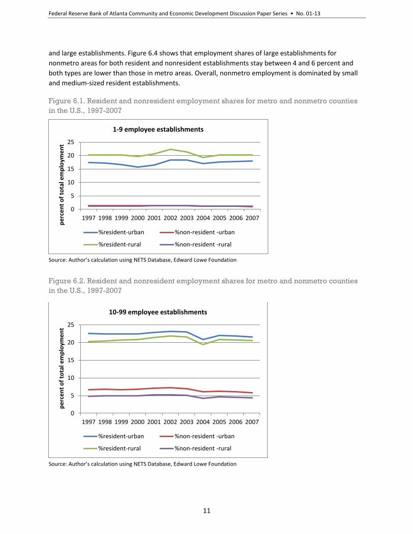
and large establishments. Figure 6.4 shows that employment shares of large establishments for
nonmetro areas for both resident and nonresident establishments stay between 4 and 6 percent and
both types are lower than those in metro areas. Overall, nonmetro employment is dominated by small
and medium-sized resident establishments.
Figure 6.1. Resident and nonresident employment shares for metro and nonmetro counties
in the U.S., 1997-2007
Source: Author’s calculation using NETS Database, Edward Lowe Foundation
Figure 6.2. Resident and nonresident employment shares for metro and nonmetro counties
in the U.S., 1997-2007
Source: Author’s calculation using NETS Database, Edward Lowe Foundation
0
5
10
15
20
25
1997 1998 1999 2000 2001 2002 2003 2004 2005 2006 2007
pe
rce
nt
of
tota
l em
plo
yme
nt
1-9 employee establishments
%resident-urban %non-resident -urban
%resident-rural %non-resident -rural
0
5
10
15
20
25
1997 1998 1999 2000 2001 2002 2003 2004 2005 2006 2007
pe
rce
nt
of
tota
l em
plo
yme
nt
10-99 employee establishments
%resident-urban %non-resident -urban
%resident-rural %non-resident -rural

Federal Reserve Bank of Atlanta Community and Economic Development Discussion Paper Series • No. 01-13
12
Figure 6.3. Resident and nonresident employment shares for metro and nonmetro counties
in the U.S., 1997-2007
Source: Author’s calculation using NETS Database, Edward Lowe Foundation
Figure 6.4. Resident and nonresident employment shares for metro and nonmetro counties
in the U.S., 1997-2007
Source: Author’s calculation using NETS Database, Edward Lowe Foundation
0
2
4
6
8
10
12
1997 1998 1999 2000 2001 2002 2003 2004 2005 2006 2007
pe
rce
nt
of
tota
l em
plo
yme
nt
100-499 employee establishments
%resident-urban %non-resident -urban
%resident-rural %non-resident -rural
0
2
4
6
8
10
12
14
1997 1998 1999 2000 2001 2002 2003 2004 2005 2006 2007
pe
rce
nt
of
tota
l em
plo
yme
nt
500 and above employee establishments
%resident-urban %non-resident -urban
%resident-rural %non-resident -rural

Federal Reserve Bank of Atlanta Community and Economic Development Discussion Paper Series • No. 01-13
13
Methodology
The empirical framework for the analysis is based on Mankiw, et al (1992), but I use a more ad hoc
regression equation (Temple, 1999) that includes a wider set of factors that affect local economic
performance. To evaluate the relationship between local entrepreneurship and economic performance
over the period 2000-2008, I use the following regression equation:
(1) yi = αi + βyit−T + γestabit−T + δ Xit−T + εi
where yi is the dependent variable under consideration for economy i during the time period T, yit−T is a
convergence variable, estabit−T is a vector of the initial employment share of resident establishments (or
a vector of their subcategories based on employment size of establishments), as a percent of total
employment, Xit−T is a vector of other initial conditions, and εi is the error term. For the dependent
variables I use county per capita real income growth, employment growth, and change in poverty rate,
between 2000 and 2008 (2009 for poverty rate). For the employment rate, I use total full- and part-time
employment in a county. What follows is a brief description of the variables used in the estimation and
their measurement.
To measure the role of resident businesses in a county, I use the NETS database on the share of
total employment accounted for by these businesses.7 In one specification of the equation (1), I use the
total employment in resident establishments as a percent of total employment by all establishments
(resall). In another specification of equation (1) I use a disaggregated shares of total resident
employment based on establishment size. I control for eight initial conditions. As in most regional
growth regressions, I include initial per capita income (rlinc), initial total full-and part-time employment
(temp), and initial poverty rate (indpov) in each of the regression equations respectively to control for
convergence effects. Other control variables include percent of people who have a college degree or
more (college) to capture human capital, local government property taxes per capita (pcptaxt), and
expenditures on education (edexp) and highways (hyexp) as policy variables, nonwhite minorities
(nonwhite) to capture recent labor market trends, population density (popden) as an agglomeration
variable and natural amenity index (amnscale).
Based on previous literature on local entrepreneurship and small business, I test the following
two major hypotheses in this study:
(1) local entrepreneurship has a positive effect on county per capita income growth and
employment growth and a negative effect on change in poverty in counties; and
(2) smaller local businesses have a more positive effect on local economic performance
(measured as per capita income growth, employment growth, and change in poverty) than
larger local businesses.
Estimation issues: endogeneity and spatial dependence
My analyses may be prone to biases resulting from endogeneity. For example faster per capita
income and employment growth might encourage the entry of more local businesses to the locality.
Michelacci and Silva (2007) find that local bias in entrepreneurship is associated with a region’s level of
7 One shortcoming of this measure, as observed by Beck et al (2005), is that it is a static measure. My data do not take into
consideration the entry of new firms, firm deaths, or growth of firms.

Federal Reserve Bank of Atlanta Community and Economic Development Discussion Paper Series • No. 01-13
14
economic development. This scenario would bias, usually upward, the parameter estimates and
explanatory power (Glaeser and Kerr, 2009). I use lag values for local entrepreneurship variables and
spatial econometric methods (described below) to mitigate the endogeneity bias in the data.
Lesage and Fischer (2008) present a strong case for using a spatial econometric approach to
estimate regional growth models. There is also a sizeable and growing literature in regional science
showing that regional growth rates exhibit spatial dependence and Abreu et al. (2004) summarizes over
50 such studies. The present study uses county-level data in the United States and many county- and
state-level studies that have been conducted to investigate income growth, poverty, and employment in
the United States use spatial econometric approach (see for example Rey and Montouri, 1999;
Rupasingha et al., 2002; Rupasingha and Goetz, 2007). Previous growth studies have used competing
spatial models to address various forms of spatial dependence. For example, some studies consider only
spatial dependence in the dependent variable using spatial lag model (SAR) and others examine only
spatial dependence in the error term using spatial error model (SEM) (Abreu, et al., 2004). Abreu et al.
(2004) also refer to studies that use both error and lag dependence in the same model using general
spatial model (SAC) as well as spatial dependence in the independent variables. Lesage and Fischer
(2008), based on the results derived in Lesage and Pace (2009), suggest that the appropriate spatial
regression model for regional growth regressions is the Spatial Durbin Model (SDM). The SDM includes a
spatial lag of the dependent variable as well as spatial lags of the explanatory variables.
The SDM for the growth model in equation (1) can be written as:
(2) yi = αi + W(yi) + βYit-T + µWYit-T + ∑ δjX ij,t−T + W∑
γj(Xij,t-T) + εi
~ N(0,2In)
where yi denotes an nx1 vector of the dependent variable (income growth, employment growth or
change in poverty in the present case) as in equation (1), Yit-T is the convergence variable, X represents
an nxk matrix containing the determinants of the dependent variable including variables for local
entrepreneurship and W is an nxn spatial weights matrix. The terms W(yi), µWYit-T , and
γW∑ (Xit−T) in the equation adds dependent variable, convergence variables, and explanatory
variables respectively from neighboring counties. , β, µ, δ, and γ denote the parameters to be
estimated. The coefficients, µ, and γ pick up the extent to which the dependent and independent
variables of nearby counties influence economic performance in the original county.
One motivation for using the SDM for growth regressions is that it is the only spatial model that
nests spatial dependence in the dependent variable, independent variables and error term that will
produce unbiased estimates (Lesage and Pace, 2009). The setting parameters µ = 0 and γ = 0 in equation
(2) leads to the SAR specification that includes a spatial lag of the dependent variable from neighboring
regions. Imposing the common factor parameter restriction γ = -δ and µ = -β yields the SEM
specification (LeSage and Pace, 2009). Also, imposing the restriction that all spatial parameters are equal
to zero yields the standard OLS regression model. Another motivation for using the SDM is that an
omitted variables problem likely arises when handling regional data samples and Lesage and Pace (2009)
demonstrate that parameter estimates of the SDM are not affected by the magnitude of the spatial
dependence in the omitted variables.

Federal Reserve Bank of Atlanta Community and Economic Development Discussion Paper Series • No. 01-13
15
Descriptive Statistics and Correlations
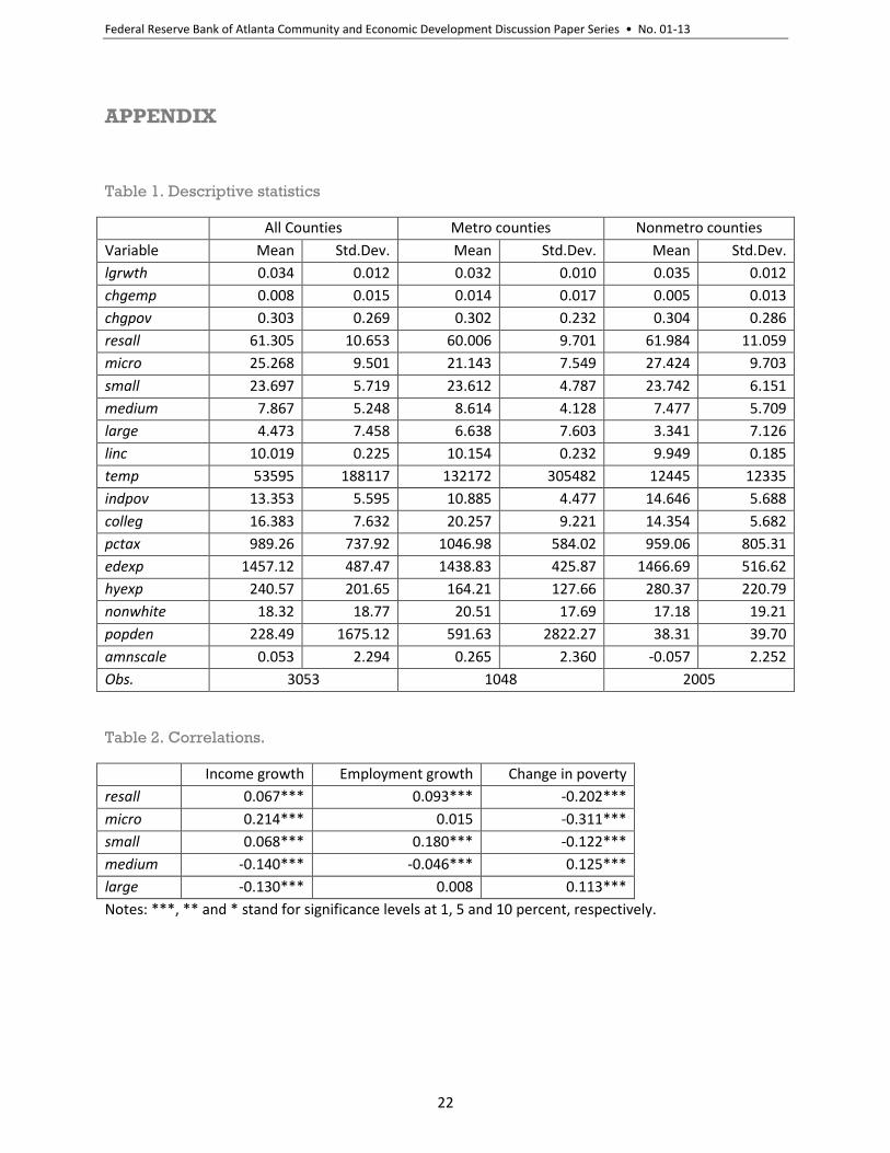
Table 1 presents summary statistics of the variables used in the analysis for all counties, metro counties,
and nonmetro counties.8 There is a wide variation in average annual real per capita income growth
across the counties in my sample over the period 2000–2008, ranging from –10.0 percent in Slope
County, North Dakota to 12 percent in Hayes County, Nebraska, with a mean of 0.8 percent and
standard deviation of 2 percent. Average annual employment growth varies from –6.0 percent in St.
Bernard Parish, Louisiana to 11 percent in Storey County, Nevada and average annual individual poverty
rate changes from –1.3 percent in Starr County, Texas, to 2.3 percent in Irwin County, Georgia. I
generally observe substantial county-level variation in the measures of initial conditions. For example,
the share of the population who have a college degree or more range from 5 percent (Edmonson
County, Kentucky) to 61 percent (Los Alamos County, New Mexico), with a mean of 16 percent and
standard deviation of 7.63 percent. The natural amenity index varies from -6.40 in Red Lake County,
Minnesota to 11.17 in Ventura County, California, with a mean of 0.27 and standard deviation of 2.4.
There is also substantial variation across counties in local government taxes and expenditure on
education and highways.
Table 2 presents the correlations between the dependent variables and the variables of interest in
this study which are percent of employment in total resident establishments and the establishment
categories based on employment size described above. For the sake of conciseness, only the statistically
significant correlations for all counties sample are discussed here. Simple correlations indicate that the
total employment share in resident establishments is positively correlated with real per capita income and
employment growth and negatively correlated with change in poverty, indicating that the resident
establishment employment share is clearly favorably correlated with local economic performance
measures. Results are mixed with respect to employment size (stages) categories. The share of
employment in micro businesses is positively correlated with income growth, negatively correlated with
change in poverty, and not significantly correlated with employment growth. The share of employment in
small resident establishments is positively correlated with income and employment growth and negatively
correlated with change in poverty. The resident share of employment in medium businesses is negatively
correlated with income and employment growth and positively correlated with change in poverty. The
resident share of employment in large establishments is negatively correlated with income growth,
positively correlated with change in poverty, and not significantly correlated with employment growth.
Econometric Estimation Results
I use three samples to estimate the model presented in equation 1 for each of my local economic
performance measures. The three samples are all counties of the United States, both metro and
nonmetro counties. For all three samples, I obtained two sets of estimates as follows. First, I include all
the initial conditions and aggregated resident employment share (set one). Second, I include all the
initial conditions and disaggregated resident employment shares based on employment size (set two).
Results are organized as follows.
I first present and discuss income growth results, followed by employment growth and change
in poverty. Each dependent variable is featured in two separate tables, one for the set-one and another
8 See Appendix for all tables.
Federal Reserve Bank of Atlanta Community and Economic Development Discussion Paper Series • No. 01-13
16
for the set-two variables. Each table has three samples: all counties, metro counties, and nonmetro
counties. Multicollinearity across the independent variables was not found to be an issue, as variance
inflation factors were consistently below 2 for all variables in income and employment growth and all
variables in change in poverty equation with the exception of 2.1 for one variable in the set-two
regression.
OLS results
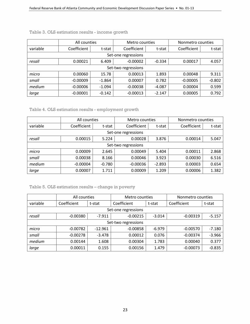
Tables 3-5 presents results of OLS estimations of equation (1) and the consistent estimates were
produced using White procedure. The results for the income growth equation with set-one and set-two
results are presented in Table 3. The resident share of employment was highly significant and positive in
all counties and nonmetro counties samples but not significant in the metro sample. Next I estimate the
income growth equation with set-two variables. Results for all counties show that among resident
employment sizes, micro business share has a positive and significant association with income growth
(significant at 1 percent), but the small business share has a negative and significant (at 10 percent)
association. Medium and large employment shares are not significant. Results for the metro sample
show that the micro establishment share is positive and significant at the 6 percent level, but medium
and large shares are negative and significant (at 1 percent and 5 percent respectively). In the nonmetro
sample only the micro employment share is significant (1 percent) and positively associated with income
growth. Other sizes are not statistically significant.
The model represented in Equation (1) is used to analyze employment growth in all U.S.
counties, metro counties, and nonmetro counties, from 2000 to 2008 and results are reported in Table 4
for set-one and set-two variables. The resident share of employment was highly significant (at 1 percent)
and positive in all samples. Next I estimate the employment growth equation with set-two variables.
Results for all counties show that among resident employment sizes, micro and small business
employment shares were significant at 1 percent and large business share was significant at the 10
percent level. All three of these parameters are positive, indicating a favorable association with
employment growth in counties. Results for the metro sample show that micro and small employment
shares have a positive and significant (at 1 percent level) association with employment growth. Medium
employment share is negative and significant (at 1 percent), indicating an unfavorable association with
employment growth in metro counties. In the nonmetro sample only micro and small employment
shares are significant (1 percent) and positively associated with employment growth. Other sizes are not
statistically significant.
Next I estimate the model represented in Equation (1) to analyze change in poverty from 2000
to 2009 and results are reported in Table 5. Regression results with set-one variables show that resident
share employment is negatively associated with change in poverty in all three samples. Estimated
parameters were significant at 1 percent for all samples. Table 5 also reports the results for set-two
variables. The share of micro and small employment shares are negative and significant (1 percent) for
all counties and nonmetro counties samples. The share of micro employment share is negative and
significant (1 percent) for the metro sample. The medium employment share is positive and significant
(10 percent) for all counties and nonmetro counties samples.

Federal Reserve Bank of Atlanta Community and Economic Development Discussion Paper Series • No. 01-13
17
Spatial model results
As pointed out above, growth models with county-level data may exhibit spatial dependence. In
this section, following Lesage and Fischer (2008) and others (Fischer, et al., 2009, LeSage and Pace,
2009), I estimate a series of SDM specifications and show that the SDM is the suitable choice among
competing spatial specifications. The estimation of the SDM is the same as the spatial lag model (SAR),
through maximum likelihood procedure, the difference being that the SDM procedure doubles the
number of independent variables in the model with the inclusion of spatially lagged independent
variables. Results presented in Tables 6-119 show that all the spatial lag parameters are statistically
significant at the 1 percent level, indicating spatial dependence in the dependent variables and
therefore the simple restriction that spatial lag parameter is equal to zero does not hold. The likelihood
ratio tests conducted to discriminate between unrestricted SDM and the SEM (Fischer, et al., 2009)
reject the common factor restriction at the 1 percent level for all specifications in all samples and
therefore the SEM specification. The significant spatial parameters in all specifications for all samples
also show that my results based on OLS may be biased, inefficient, and inconsistent (Anselin, 1988).
Also notable in Tables 6-11 is that there are many statistically significant spatially-lagged initial
conditions in all specifications, indicating that characteristics of neighboring counties do play a role in
explaining the economic performance of a particular county. If the coefficients of my variables of
interest in the OLS model and the SDM are to be compared, the parameter estimates for most of the
resident employment shares were not changed in terms of signs and general significance levels. Affected
resident employment shares were as follows. In the income growth model, medium employment share
is significant and large employment share is not significant in the OLS for all counties, micro and large
employment shares were significant in the OLS for metro counties, and medium share is not significant
in the OLS for nonmetro counties. In the employment growth model, large share is not significant for
metro counties. In the change in poverty model, total resident share and medium share of employment
are significant in the OLS model. Overall, the estimation results on resident employment shares support
my a priori hypothesis that resident/local establishment employment shares are associated with better
local economic performance and when disaggregated, higher shares of smaller resident businesses are
associated with better county economic performance.
The interpretation of estimated parameters in the SDM estimation is richer and more
complicated due to the fact that spatial models expand the information set to include the information
on neighboring regions (LeSage and Pace, 2009). Therefore the least squares simple partial derivative
interpretation of regression parameters does not hold any more in the SDM context. For example, in my
SDM setting, the per capita income growth in county i depends on the income growth of county i's
neighboring counties, county i's initial per capita income, initial per capita income of neighboring
counties, county i's other initial conditions including local entrepreneurship shares, and other initial
conditions of neighboring counties. LeSage and Pace (2009) demonstrate that a change in a single
explanatory variable in region i has a ‘direct effect’ on region i as well an ‘indirect effect’ on i's
neighboring counties. Lesage and Pace (2009) point out that there are two ways to interpret indirect
impacts: the impact a region has on all other regions and the impact of all other regions on a particular
9 I standardized each dependent and independent variable by subtracting its mean and dividing by its standard deviation to
avoid badly conditioned variables and negative definite matrices.

Federal Reserve Bank of Atlanta Community and Economic Development Discussion Paper Series • No. 01-13
18
region. I rely on LeSage and Pace (2009) to interpret correctly the impact of local entrepreneurship on
measures of county economic performance.10
Tables 12-17 present the summary direct and indirect impact measures for my SDM
specification for set-one and set-two variables for all samples. A comparison between the model
average estimates presented in Tables 6-11 and the direct impact estimates presented in Tables 12-17
shows that in some cases these estimates are similar in magnitudes, while others are different in
magnitude. The reason for these differences is due to feedback effects (Lesage and Fischer, 2008). For
example, while the coefficient estimates seem to be similar in magnitude for amenity scale in income
growth equation for all counties model (-0.088 and -0.088, respectively for average estimate and direct
estimate), they seem to differ in magnitude for per capita property taxes (0.139 and 0.170, respectively
for average estimate and direct estimate).
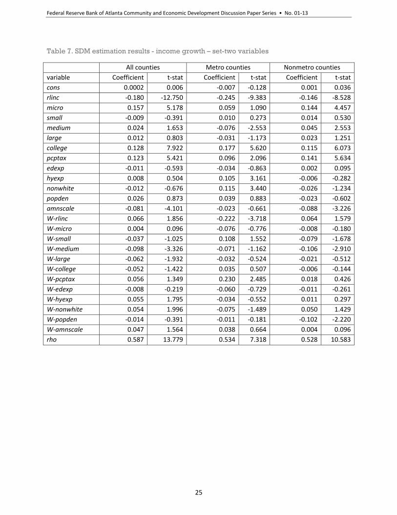
Income growth
The direct and indirect impact measures for the income growth equation for all samples are
presented in Table 12 for set-one variables and Table 13 for set-two variables. Turning to the direct
impact of total resident employment share on county real per capita income growth, it has a positive
and significant impact for all counties and nonmetro samples, but has no significant effect for metro
sample. When disaggregated to establishment size, the share of employment in micro establishments is
positive and significant for all counties and nonmetro samples. The medium share is negative and
significant for metro sample and positive and significant for the nonmetro sample. While I do not
observe any significant indirect impact of aggregate resident employment share, few estimates in set-
two regression are significant. The micro share is positive and medium and large shares are negative in
the all counties sample and medium share is negative in the nonmetro sample. The positive and
significant indirect impact of the micro share in the all counties sample can be interpreted as: one
percent increase in the share of micro employment in a county will on average result in all other
counties collectively experiencing a 0.23 percent increase in real per capita income. This can also be
interpreted as a one percent increase in micro share in all other counties will on average lead to a 0.23
percent increase in real per capita income for a particular county.
The direct impacts of the rest of the control variables11 have generally been as expected. Initial
per capita income is negative and highly significant for all samples in both set-one and set-two
regressions. The estimate for the percentage of the population with at least a bachelor’s degree is
positive and significant in all samples and highly significant for all samples in both set-one and set-two
regressions. The estimate for the per capita property tax variable is significant with an unexpected
positive sign for all samples in both set-one and set-two regressions. While the estimate for government
expenditure on education is not significant in any of the specifications, the estimate for per capita
expenditure on highways is positive and significant for the all counties and metro samples in set-one
regression and positive and significant for metro sample in set-two regression. The nonwhite estimate is
significant and negative for the all counties and nonmetro samples, but significant and positive for
metro counties in set-one regression. This estimate in significant only in the metro sample and is
10
See LeSage and Pace (2009) and others (Fischer, et al., 2009; Lesage and Fischer, 2008) for details regarding the specific calculations. 11
For the sake of brevity, we only discuss here the direct effects of these variables and interested readers may consult Tables 12-17 for details.

Federal Reserve Bank of Atlanta Community and Economic Development Discussion Paper Series • No. 01-13
19
positive in set-two regression. The estimate for population density is only significant for nonmetro
sample in set-one regression and is negative. The estimate for natural amenity index is negative and
significant for the all counties and nonmetro samples in set-one and set-two regressions.
Employment growth
The direct and indirect impact measures for the employment growth equation for all samples
are present in Table 14 for set-one variables and Table 15 for set-two variables. The aggregate resident
share of employment has a positive and significant impact for all samples. When disaggregated to
establishment size, the shares of employment in micro and small establishments are positive and
significant for all samples. The medium share is negative and significant for the metro sample and the
large share is positive and significant in the all counties and metro samples. Indirect impact estimates for
all employment shares, except the micro share, in employment growth equation for the all counties
model are not significant. The micro share in employment growth equation for the all counties sample is
negative and significant indicating that the feedback effects of this particular variable are negative from
a particular county to rest of the counties and vice versa.
I now turn to a brief discussion of the direct impacts of the rest of the control variables in
employment growth equation. The estimated convergence parameter (initial employment level in a
county) has the expected negative sign and is significant in all specifications except for the nonmetro
sample, where it is not statistically significant. The estimated parameter for the education variable is
positive and significant in all regressions. Per capita property taxes enter negatively and significantly for
the all counties and metro samples, but not for the nonmetro sample. The direct impact estimate for per
capita education expenditure indicates no significant association with employment growth in any
specification. A negative and highly significant association is shown for per capita government
expenditure on highways for the all counties and nonmetro samples. The direct impact estimate for the
nonwhite variable is negative and significant in the all counties and metro samples and positive and
significant in the nonmetro sample. Population density estimate shows no statistically significant
association with employment growth in any sample. The natural amenity scale estimate is significant
and positive for the nonmetro sample only.
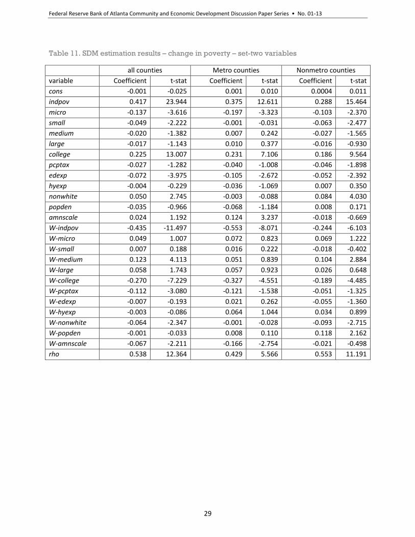
Change in poverty regressions
The direct and indirect impact measures for change in the poverty equation for all samples are
present in Table 16 for set-one variables and Table 17 for set-two variables. The aggregate resident
share of employment has a negative and significant direct impact for the all counties and nonmetro
samples, indicating that this measure has a favorable association with poverty reduction in respective
regions. This estimate is not significant in the metro sample. As for the direct impact of disaggregated
resident employment shares, the micro share is negative and significant for all samples. And the small
share is negative and significant for the all counties and nonmetro samples. Turning to indirect effects of
the variables of interest, only the medium share estimate is significant, and that is for the all counties
and nonmetro samples. This estimate has a positive sign, showing that the feedback effects of this
particular variable from a particular county to rest of the counties and vice versa are not favorable for
poverty reduction.
Signs and significant levels of the direct impact measure for rest of the control variables in the
poverty regressions, in general, are as expected except for the initial poverty level (convergence

Federal Reserve Bank of Atlanta Community and Economic Development Discussion Paper Series • No. 01-13
20
variable) and education variables. The parameter estimates for both of these variables are consistently
significant across all specifications for all three samples, but have a positive sign. A positive and
significant initial poverty rate estimate indicates that counties that had higher initial poverty have gotten
poorer over the study period. The positive sign for the estimate for the education variable is against the
conventional belief. The direct impact of per capita property taxes is negative and significant in the all
counties and nonmetro samples. The estimate for per capita expenditure on education is negative and
significant for all specifications. The highway expenditure estimate is negative and significant only for
the metro sample with set-one variables. The estimate for the nonwhite variable is positive and
significant for all samples with set-one specification and for the all counties and nonmetro samples with
set-two specification. The estimate for population density is not significant in any of the specifications
and the estimate for the natural amenity index is positive and significant for the metro sample.
Endogeneity bias
As mentioned above, my results could be subject to endogeneity bias and I have attempted to
address this issue in my estimation methods. First, I use initial or beginning period values of resident and
nonresident businesses, which is known as a weakly exogenous regressors approach (Levine, et al.,
2000). Lagged values from year 2000 were also used for other explanatory variables in order to mitigate
the potential endogeneity issues associated with those variables. I also test this further by including
lagged employment shares of 1997, which is prior to my initial year of 2000, considering the fact that my
initial employment shares may be subject to a greater level of stochastic disturbance over short time
period. The results (not reported here) remained unchanged for coefficients and significance levels with
the use of 1997 values for local employment shares. Another way that I correct the endogeneity bias in
my data is with the use of SDM. A main concern for endogeneity arises when there are omitted variables
that exhibit non-zero covariance with variables included in the model. The use of the SDM for the
analysis minimizes this problem (Brasington and Hite, 2005) because the SDM controls for the influence
of omitted variables, thus alleviating the need to instrument for endogenous variables.
Summary and Conclusions
This study presents preliminary evidence on the effects of local entrepreneurship on local economic
performance. Exploiting a rich county-level variation in locally-owned businesses and economic
performance variables, I conducted a systematic investigation into the significance of local
entrepreneurship for local economic performance in the United States at the county-level. The
conceptual framework followed a conventional conditional growth model to study the effects of local
entrepreneurship on real per capita income growth, employment growth, and change in poverty for all
counties in the United States. I also estimated the models for metro and nonmetro. The estimation
approach used an OLS, corrected for heteroskedasticity, and spatial econometric method that utilizes a
Spatial Durbin Model. I addressed possible endogeneity bias in my data. Two main hypotheses were
tested with the estimation. They are: (1) local entrepreneurship in general has a positive effect on
county per capita income growth and employment growth and a negative effect on change in poverty in
counties; and (2) smaller local businesses have a more positive effect on local economic performance
(measured as per capita income growth, employment growth, and change in poverty) than larger local
businesses.

Federal Reserve Bank of Atlanta Community and Economic Development Discussion Paper Series • No. 01-13
21
My results in general support the two main hypotheses and provide evidence that local
entrepreneurship matters for local economic performance and smaller local businesses are more
conducive than larger local businesses for local economic performance. Results are quite robust to the
inclusion of other commonly used control variables in regional growth models, the incorporation of
spatial dependence in the data, and the estimation of sub-samples for metro and nonmetro counties. I
find that the percent of employment provided by resident, or locally-owned, business establishments
has a significant positive effect on county income and employment growth and a significant and
negative effect on change in poverty in the all counties and nonmetro counties samples. When
disaggregated the employment share of resident businesses to establishment size, the results show that
smaller resident establishments are more favorable for county economic performance. For example, the
micro employment share is positive and significant for income growth for the all counties and nonmetro
counties samples. The same estimate is positive and significant in employment growth and negative and
significant in change in poverty for all samples that I estimated. The share of employment in small
establishments has a positive and significant association with employment growth for all samples and a
negative and significant association with change in poverty for the all counties and nonmetro samples.
The effects of the employment shares in medium and large businesses are mixed. For example, the
medium share is negative and significant on income growth for the metro sample and positive and
significant on income growth for the nonmetro sample. In the employment growth equation, the
medium share is negative and significant for the metro sample and the large share is positive and
significant for the all counties and metro samples. The poverty regressions show no clear effects of
medium and large establishments. These findings clearly show that employment in micro and small-
sized local establishments are favorable for county income and employment growth and poverty
reduction. However, the effects of employment in larger resident establishments on local economies are
mixed.
Supporting the expectations of policy makers, some researchers and economic development
practitioners, I find evidence that locally-based business development may be a viable local economic
development approach. More specifically, I find evidence that higher percentages of employment in
locally-based, micro and small-sized businesses are more favorable for local economies. Based on my
results, the evidence for the effects of medium- and large-sized establishments is ambiguous. My results
suggest that fostering smaller local businesses may be good local economic development policy. While
more research is needed to identify the primary needs of local entrepreneurs, local policy makers and
economic development practitioners may want to consider strategic interventions to help local small
business owners by addressing barriers such as access to technology and capital by building and
investing in entrepreneurship-friendly ecosystems. Though, my study does not shed light on the efficacy
of specific policies to stimulate local entrepreneurship. Of course, my findings are only preliminary and
additional studies are necessary to substantiate these findings. This may require conducting panel
studies, establishing stronger causal relationships, and also examining the industrial composition and
dynamics of these local businesses.
Federal Reserve Bank of Atlanta Community and Economic Development Discussion Paper Series • No. 01-13
22
APPENDIX
Table 1. Descriptive statistics
All Counties Metro counties Nonmetro counties
Variable Mean Std.Dev. Mean Std.Dev. Mean Std.Dev.
lgrwth 0.034 0.012 0.032 0.010 0.035 0.012
chgemp 0.008 0.015 0.014 0.017 0.005 0.013
chgpov 0.303 0.269 0.302 0.232 0.304 0.286
resall 61.305 10.653 60.006 9.701 61.984 11.059
micro 25.268 9.501 21.143 7.549 27.424 9.703
small 23.697 5.719 23.612 4.787 23.742 6.151
medium 7.867 5.248 8.614 4.128 7.477 5.709
large 4.473 7.458 6.638 7.603 3.341 7.126
linc 10.019 0.225 10.154 0.232 9.949 0.185
temp 53595 188117 132172 305482 12445 12335
indpov 13.353 5.595 10.885 4.477 14.646 5.688
colleg 16.383 7.632 20.257 9.221 14.354 5.682
pctax 989.26 737.92 1046.98 584.02 959.06 805.31
edexp 1457.12 487.47 1438.83 425.87 1466.69 516.62
hyexp 240.57 201.65 164.21 127.66 280.37 220.79
nonwhite 18.32 18.77 20.51 17.69 17.18 19.21
popden 228.49 1675.12 591.63 2822.27 38.31 39.70
amnscale 0.053 2.294 0.265 2.360 -0.057 2.252
Obs. 3053 1048 2005
Table 2. Correlations.
Income growth Employment growth Change in poverty
resall 0.067*** 0.093*** -0.202***
micro 0.214*** 0.015 -0.311***
small 0.068*** 0.180*** -0.122***
medium -0.140*** -0.046*** 0.125***
large -0.130*** 0.008 0.113***
Notes: ***, ** and * stand for significance levels at 1, 5 and 10 percent, respectively.
Federal Reserve Bank of Atlanta Community and Economic Development Discussion Paper Series • No. 01-13
23
Table 3. OLS estimation results - income growth
All counties Metro counties Nonmetro counties
variable Coefficient t-stat Coefficient t-stat Coefficient t-stat
Set-one regressions
resall 0.00021 6.409 -0.00002 -0.334 0.00017 4.057
Set-two regressions
micro 0.00060 15.78 0.00013 1.893 0.00048 9.311
small -0.00009 -1.864 0.00007 0.782 -0.00005 -0.802
medium -0.00006 -1.094 -0.00038 -4.087 0.00004 0.599
large -0.00001 -0.142 -0.00013 -2.147 0.00005 0.792
Table 4. OLS estimation results - employment growth
All counties Metro counties Nonmetro counties
variable Coefficient t-stat Coefficient t-stat Coefficient t-stat
Set-one regressions
resall 0.00015 5.224 0.00028 3.876 0.00014 5.047
Set-two regressions
micro 0.00009 2.645 0.00049 5.404 0.00011 2.868
small 0.00038 8.166 0.00046 3.923 0.00030 6.516
medium -0.00004 -0.780 -0.00036 -2.893 0.00003 0.654
large 0.00007 1.711 0.00009 1.209 0.00006 1.382
Table 5. OLS estimation results – change in poverty
All counties Metro counties Nonmetro counties
variable Coefficient t-stat Coefficient t-stat Coefficient t-stat
Set-one regressions
resall -0.00380 -7.911 -0.00215 -3.014 -0.00319 -5.157
Set-two regressions
micro -0.00782 -12.961 -0.00858 -6.979 -0.00570 -7.180
small -0.00278 -3.478 0.00012 0.076 -0.00374 -3.966
medium 0.00144 1.608 0.00304 1.783 0.00040 0.377
large 0.00011 0.155 0.00156 1.479 -0.00073 -0.835

Federal Reserve Bank of Atlanta Community and Economic Development Discussion Paper Series • No. 01-13
24
Table 6. SDM estimation results - income growth – set-one variables
All counties Metro counties Nonmetro counties
variable Coefficient t-stat Coefficient t-stat Coefficient t-stat
cons 0.000 -0.003 -0.006 -0.108 0.001 0.026
rlinc -0.214 -14.740 -0.263 -9.896 -0.160 -9.220
resall 0.070 2.345 -0.004 -0.072 0.083 2.631
college 0.112 7.333 0.163 5.853 0.111 5.831
pcptax 0.139 6.156 0.082 1.797 0.146 5.872
edexp -0.011 -0.601 -0.029 -0.760 0.004 0.168
hyexp 0.024 1.457 0.123 3.713 -0.004 -0.183
nonwhite -0.068 -3.813 0.056 1.704 -0.069 -3.283
popden 0.026 0.930 0.035 0.868 -0.047 -1.291
amnscale -0.088 -4.394 -0.015 -0.419 -0.094 -3.490
W-rlinc 0.031 0.877 -0.234 -3.893 0.087 2.123
W-resall -0.013 -0.302 0.016 0.162 -0.068 -1.476
W-college -0.027 -0.933 0.072 1.284 0.012 0.310
W-pcptax 0.097 2.358 0.243 2.631 0.014 0.338
W-edexp 0.002 0.064 -0.087 -1.048 -0.0002 -0.004
W-hyexp 0.058 1.916 -0.039 -0.632 -0.023 -0.610
W-nonwhite 0.085 3.171 -0.007 -0.144 0.075 2.183
W-popden -0.042 -1.249 -0.031 -0.559 -0.166 -3.746
W-amnscale 0.057 1.904 0.042 0.741 -0.003 -0.067
rho 0.633 14.656 0.561 7.652 0.547 10.899
Federal Reserve Bank of Atlanta Community and Economic Development Discussion Paper Series • No. 01-13
25
Table 7. SDM estimation results - income growth – set-two variables
All counties Metro counties Nonmetro counties
variable Coefficient t-stat Coefficient t-stat Coefficient t-stat
cons 0.0002 0.006 -0.007 -0.128 0.001 0.036
rlinc -0.180 -12.750 -0.245 -9.383 -0.146 -8.528
micro 0.157 5.178 0.059 1.090 0.144 4.457
small -0.009 -0.391 0.010 0.273 0.014 0.530
medium 0.024 1.653 -0.076 -2.553 0.045 2.553
large 0.012 0.803 -0.031 -1.173 0.023 1.251
college 0.128 7.922 0.177 5.620 0.115 6.073
pcptax 0.123 5.421 0.096 2.096 0.141 5.634
edexp -0.011 -0.593 -0.034 -0.863 0.002 0.095
hyexp 0.008 0.504 0.105 3.161 -0.006 -0.282
nonwhite -0.012 -0.676 0.115 3.440 -0.026 -1.234
popden 0.026 0.873 0.039 0.883 -0.023 -0.602
amnscale -0.081 -4.101 -0.023 -0.661 -0.088 -3.226
W-rlinc 0.066 1.856 -0.222 -3.718 0.064 1.579
W-micro 0.004 0.096 -0.076 -0.776 -0.008 -0.180
W-small -0.037 -1.025 0.108 1.552 -0.079 -1.678
W-medium -0.098 -3.326 -0.071 -1.162 -0.106 -2.910
W-large -0.062 -1.932 -0.032 -0.524 -0.021 -0.512
W-college -0.052 -1.422 0.035 0.507 -0.006 -0.144
W-pcptax 0.056 1.349 0.230 2.485 0.018 0.426
W-edexp -0.008 -0.219 -0.060 -0.729 -0.011 -0.261
W-hyexp 0.055 1.795 -0.034 -0.552 0.011 0.297
W-nonwhite 0.054 1.996 -0.075 -1.489 0.050 1.429
W-popden -0.014 -0.391 -0.011 -0.181 -0.102 -2.220
W-amnscale 0.047 1.564 0.038 0.664 0.004 0.096
rho 0.587 13.779 0.534 7.318 0.528 10.583

Federal Reserve Bank of Atlanta Community and Economic Development Discussion Paper Series • No. 01-13
26
Table 8. SDM estimation results - employment growth – set-one variables
All counties Metro counties Nonmetro counties
variable Coefficient t-stat Coefficient t-stat Coefficient t-stat
cons 0.002 0.048 0.004 0.060 0.0002 0.004
temp -0.123 -7.961 -0.154 -5.640 -0.001 -0.044
resall 0.098 4.902 0.126 3.566 0.103 3.120
college 0.227 12.894 0.227 7.685 0.170 7.746
pcptax -0.071 -3.212 -0.111 -2.883 -0.013 -0.453
edexp -0.008 -0.395 0.054 1.295 -0.038 -1.509
hyexp -0.078 -4.207 -0.030 -0.844 -0.073 -3.203
nonwhite -0.144 -7.223 -0.303 -7.994 0.050 1.998
popden -0.024 -0.815 -0.002 -0.049 0.028 0.694
amnscale 0.001 0.025 -0.046 -1.130 0.085 2.144
W-temp 0.165 4.045 0.168 2.543 -0.035 -0.742
W-resall -0.055 -1.456 -0.065 -0.953 0.033 0.542
W-college -0.089 -2.705 -0.164 -2.806 -0.108 -2.457
W-pcptax 0.065 1.795 0.136 1.902 0.033 0.747
W-edexp -0.020 -0.539 -0.130 -1.568 0.068 1.475
W-hyexp -0.010 -0.287 0.021 0.323 0.034 0.758
W-nonwhite 0.188 6.174 0.424 7.526 -0.024 -0.585
W-popden -0.012 -0.342 -0.069 -1.109 0.049 1.028
W-amnscale 0.141 3.866 0.125 1.903 0.166 2.584
rho 0.443 9.409 0.418 5.337 0.367 6.450

Federal Reserve Bank of Atlanta Community and Economic Development Discussion Paper Series • No. 01-13
27
Table 9. SDM estimation results - employment growth – set-two variables
all counties Metro counties Nonmetro counties
variable Coefficient t-stat Coefficient t-stat Coefficient t-stat
cons 0.002 0.042 0.002 0.036 0.0004 0.010
temp -0.116 -7.596 -0.133 -4.996 0.009 0.477
micro 0.089 4.520 0.163 4.615 0.078 2.303
small 0.122 5.034 0.106 2.602 0.126 4.087
medium -0.022 -1.300 -0.065 -1.984 0.009 0.453
large 0.032 1.940 0.065 2.232 0.024 1.134
college 0.235 12.599 0.253 7.546 0.166 7.538
pcptax -0.066 -2.852 -0.087 -2.204 -0.007 -0.265
edexp -0.002 -0.090 0.046 1.110 -0.029 -1.134
hyexp -0.082 -4.460 -0.047 -1.313 -0.072 -3.165
nonwhite -0.113 -5.619 -0.232 -6.213 0.061 2.431
popden -0.021 -0.672 -0.003 -0.062 0.033 0.789
amnscale -0.008 -0.328 -0.065 -1.616 0.078 1.977
W-temp 0.147 3.649 0.194 2.950 -0.057 -1.213
W-micro -0.108 -2.759 -0.116 -1.656 -0.007 -0.114
W-small -0.015 -0.381 0.047 0.621 0.021 0.379
W-medium -0.010 -0.302 -0.063 -0.948 0.028 0.653
W-large -0.001 -0.032 -0.112 -1.730 0.052 1.122
W-college -0.101 -2.486 -0.180 -2.477 -0.099 -1.989
W-pcptax 0.056 1.516 0.112 1.554 0.017 0.386
W-edexp -0.011 -0.293 -0.105 -1.291 0.074 1.608
W-hyexp 0.001 0.022 0.009 0.138 0.029 0.648
W-nonwhite 0.145 4.717 0.336 5.990 -0.047 -1.153
W-popden -0.013 -0.339 -0.053 -0.833 0.036 0.721
W-amnscale 0.143 3.967 0.120 1.850 0.167 2.589
rho 0.446 9.517 0.392 5.059 0.360 6.355

Federal Reserve Bank of Atlanta Community and Economic Development Discussion Paper Series • No. 01-13
28
Table 10. SDM estimation results – change in poverty – set-one variables
All counties Metro counties Nonmetro counties
variable Coefficient t-stat Coefficient t-stat Coefficient t-stat
cons -0.001 -0.029 -0.001 -0.024 0.001 0.017
indpov 0.386 22.768 0.365 12.248 0.266 14.520
resall -0.090 -2.442 -0.076 -1.325 -0.084 -1.960
college 0.242 13.638 0.278 8.658 0.186 9.115
pcptax -0.035 -1.669 -0.012 -0.298 -0.051 -2.108
edexp -0.070 -3.828 -0.117 -2.949 -0.048 -2.248
hyexp -0.015 -0.930 -0.072 -2.118 0.004 0.226
nonwhite 0.108 5.965 0.097 2.766 0.122 5.813
popden -0.030 -0.873 -0.059 -1.074 0.024 0.548
amnscale 0.028 1.372 0.111 2.883 -0.016 -0.635
W-indpov -0.492 -12.760 -0.580 -8.365 -0.263 -6.535
W-resall 0.036 0.769 0.061 0.696 0.048 0.860
W-college -0.305 -9.869 -0.381 -6.344 -0.217 -5.725
W-pcptax -0.158 -4.428 -0.150 -1.909 -0.071 -1.887
W-edexp -0.002 -0.071 0.066 0.818 -0.045 -1.122
W-hyexp -0.008 -0.248 0.085 1.385 0.049 1.315
W-nonwhite -0.078 -2.904 -0.085 -1.639 -0.113 -3.338
W-popden 0.023 0.556 0.029 0.381 0.127 2.433
W-amnscale -0.066 -2.209 -0.156 -2.562 -0.016 -0.422
rho 0.568 12.931 0.453 5.830 0.566 11.464
Federal Reserve Bank of Atlanta Community and Economic Development Discussion Paper Series • No. 01-13
29
Table 11. SDM estimation results – change in poverty – set-two variables
all counties Metro counties Nonmetro counties
variable Coefficient t-stat Coefficient t-stat Coefficient t-stat
cons -0.001 -0.025 0.001 0.010 0.0004 0.011
indpov 0.417 23.944 0.375 12.611 0.288 15.464
micro -0.137 -3.616 -0.197 -3.323 -0.103 -2.370
small -0.049 -2.222 -0.001 -0.031 -0.063 -2.477
medium -0.020 -1.382 0.007 0.242 -0.027 -1.565
large -0.017 -1.143 0.010 0.377 -0.016 -0.930
college 0.225 13.007 0.231 7.106 0.186 9.564
pcptax -0.027 -1.282 -0.040 -1.008 -0.046 -1.898
edexp -0.072 -3.975 -0.105 -2.672 -0.052 -2.392
hyexp -0.004 -0.229 -0.036 -1.069 0.007 0.350
nonwhite 0.050 2.745 -0.003 -0.088 0.084 4.030
popden -0.035 -0.966 -0.068 -1.184 0.008 0.171
amnscale 0.024 1.192 0.124 3.237 -0.018 -0.669
W-indpov -0.435 -11.497 -0.553 -8.071 -0.244 -6.103
W-micro 0.049 1.007 0.072 0.823 0.069 1.222
W-small 0.007 0.188 0.016 0.222 -0.018 -0.402
W-medium 0.123 4.113 0.051 0.839 0.104 2.884
W-large 0.058 1.743 0.057 0.923 0.026 0.648
W-college -0.270 -7.229 -0.327 -4.551 -0.189 -4.485
W-pcptax -0.112 -3.080 -0.121 -1.538 -0.051 -1.325
W-edexp -0.007 -0.193 0.021 0.262 -0.055 -1.360
W-hyexp -0.003 -0.086 0.064 1.044 0.034 0.899
W-nonwhite -0.064 -2.347 -0.001 -0.028 -0.093 -2.715
W-popden -0.001 -0.033 0.008 0.110 0.118 2.162
W-amnscale -0.067 -2.211 -0.166 -2.754 -0.021 -0.498
rho 0.538 12.364 0.429 5.566 0.553 11.191

Federal Reserve Bank of Atlanta Community and Economic Development Discussion Paper Series • No. 01-13
30
Table 12. Direct and indirect effects - income growth – set-one variables
Direct effects
all counties Metro counties Nonmetro counties
Coefficient t-stat Coefficient t-stat Coefficient t-stat
rlinc -0.232 -12.463 -0.318 -8.302 -0.162 -8.420
resall 0.075 2.495 -0.005 -0.092 0.081 2.564
college 0.119 7.301 0.184 5.801 0.121 5.845
pcptax 0.170 7.220 0.122 2.530 0.158 6.325
edexp -0.012 -0.632 -0.043 -1.047 0.006 0.242
hyexp 0.035 2.086 0.127 3.578 -0.007 -0.369
nonwhite -0.061 -3.457 0.058 1.776 -0.064 -3.089
popden 0.021 0.846 0.031 0.810 -0.071 -2.015
amnscale -0.088 -4.684 -0.011 -0.321 -0.101 -3.936
Indirect effects
rlinc -0.286 -1.903 -0.881 -2.520 -0.008 -0.081
resall 0.088 0.927 0.037 0.180 -0.042 -0.510
college 0.114 1.460 0.365 2.345 0.150 1.683
pcptax 0.484 4.231 0.639 2.731 0.197 2.389
edexp -0.014 -0.172 -0.238 -1.262 0.004 0.047
hyexp 0.192 2.357 0.075 0.561 -0.055 -0.660
nonwhite 0.111 1.905 0.058 0.574 0.080 1.199
popden -0.065 -1.109 -0.028 -0.300 -0.409 -4.560
amnscale 0.001 0.022 0.079 0.746 -0.111 -1.537

Federal Reserve Bank of Atlanta Community and Economic Development Discussion Paper Series • No. 01-13
31
Table 13. Direct and indirect effects - income growth – set-two variables
Direct effects
all counties Metro counties Nonmetro counties
Coefficient t-stat Coefficient t-stat Coefficient t-stat
rlinc -0.186 -10.817 -0.291 -7.895 -0.148 -7.919
micro 0.171 5.788 0.052 0.972 0.152 4.885
small -0.014 -0.647 0.024 0.648 0.006 0.215
medium 0.012 0.778 -0.088 -2.780 0.036 1.956
large 0.003 0.212 -0.036 -1.260 0.022 1.143
college 0.131 7.082 0.193 5.545 0.122 5.960
pcptax 0.142 6.202 0.134 2.807 0.151 5.992
edexp -0.013 -0.683 -0.044 -1.052 0.002 0.089
hyexp 0.017 1.004 0.108 3.104 -0.005 -0.270
nonwhite -0.005 -0.300 0.114 3.483 -0.021 -0.983
popden 0.027 0.977 0.041 0.991 -0.034 -0.946
amnscale -0.083 -4.248 -0.020 -0.595 -0.094 -3.599
Indirect effects
rlinc -0.101 -0.890 -0.767 -2.578 -0.032 -0.324
micro 0.226 2.234 -0.085 -0.433 0.137 1.602
small -0.100 -1.323 0.234 1.558 -0.142 -1.570
medium -0.193 -2.800 -0.235 -1.584 -0.167 -2.206
large -0.134 -1.823 -0.101 -0.785 -0.013 -0.158
college 0.054 0.609 0.277 1.657 0.109 1.160
pcptax 0.296 3.242 0.583 2.766 0.186 2.390
edexp -0.029 -0.391 -0.164 -0.876 -0.016 -0.194
hyexp 0.137 1.999 0.056 0.417 0.015 0.201
nonwhite 0.111 1.987 -0.020 -0.209 0.073 1.129
popden 0.0003 0.005 0.020 0.219 -0.232 -3.295
amnscale -0.001 -0.011 0.049 0.519 -0.084 -1.066
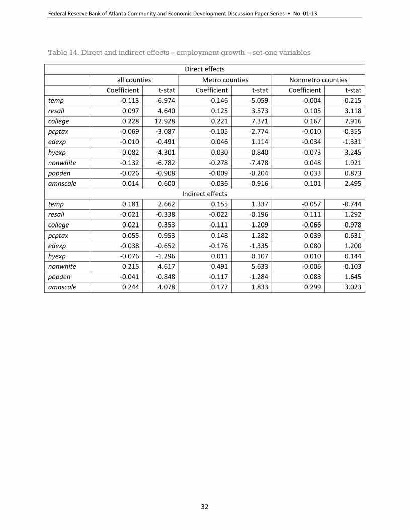
Federal Reserve Bank of Atlanta Community and Economic Development Discussion Paper Series • No. 01-13
32
Table 14. Direct and indirect effects – employment growth – set-one variables
Direct effects
all counties Metro counties Nonmetro counties
Coefficient t-stat Coefficient t-stat Coefficient t-stat
temp -0.113 -6.974 -0.146 -5.059 -0.004 -0.215
resall 0.097 4.640 0.125 3.573 0.105 3.118
college 0.228 12.928 0.221 7.371 0.167 7.916
pcptax -0.069 -3.087 -0.105 -2.774 -0.010 -0.355
edexp -0.010 -0.491 0.046 1.114 -0.034 -1.331
hyexp -0.082 -4.301 -0.030 -0.840 -0.073 -3.245
nonwhite -0.132 -6.782 -0.278 -7.478 0.048 1.921
popden -0.026 -0.908 -0.009 -0.204 0.033 0.873
amnscale 0.014 0.600 -0.036 -0.916 0.101 2.495
Indirect effects
temp 0.181 2.662 0.155 1.337 -0.057 -0.744
resall -0.021 -0.338 -0.022 -0.196 0.111 1.292
college 0.021 0.353 -0.111 -1.209 -0.066 -0.978
pcptax 0.055 0.953 0.148 1.282 0.039 0.631
edexp -0.038 -0.652 -0.176 -1.335 0.080 1.200
hyexp -0.076 -1.296 0.011 0.107 0.010 0.144
nonwhite 0.215 4.617 0.491 5.633 -0.006 -0.103
popden -0.041 -0.848 -0.117 -1.284 0.088 1.645
amnscale 0.244 4.078 0.177 1.833 0.299 3.023

Federal Reserve Bank of Atlanta Community and Economic Development Discussion Paper Series • No. 01-13
33
Table 15. Direct and indirect effects – employment growth – set-two variables
Direct effects
All counties Metro counties Nonmetro counties
Coefficient t-stat Coefficient t-prob Coefficient t-prob
temp -0.108 -6.660 -0.122 -4.436 0.006 0.290
micro 0.084 4.389 0.158 4.338 0.081 2.442
small 0.126 5.299 0.116 2.783 0.132 4.380
medium -0.024 -1.425 -0.074 -2.263 0.010 0.492
large 0.034 1.996 0.058 1.858 0.029 1.301
college 0.236 11.801 0.246 6.954 0.163 7.019
pcptax -0.063 -2.778 -0.081 -2.034 -0.007 -0.262
edexp -0.003 -0.153 0.039 0.965 -0.023 -0.901
hyexp -0.084 -4.483 -0.047 -1.328 -0.072 -3.141
nonwhite -0.103 -5.292 -0.212 -5.776 0.059 2.366
popden -0.026 -0.835 -0.006 -0.142 0.037 0.900
amnscale 0.006 0.264 -0.056 -1.437 0.092 2.356
Indirect effects
temp 0.158 2.281 0.210 2.096 -0.086 -1.105
micro -0.117 -1.873 -0.083 -0.789 0.022 0.238
small 0.069 1.067 0.143 1.155 0.102 1.220
medium -0.034 -0.606 -0.147 -1.327 0.043 0.688
large 0.023 0.389 -0.134 -1.265 0.099 1.374
college 0.011 0.147 -0.124 -1.055 -0.054 -0.697
pcptax 0.043 0.756 0.118 1.099 0.023 0.378
edexp -0.020 -0.335 -0.136 -1.096 0.097 1.452
hyexp -0.062 -1.044 -0.009 -0.089 0.008 0.125
nonwhite 0.160 3.488 0.389 4.643 -0.036 -0.641
popden -0.040 -0.797 -0.090 -1.034 0.073 1.256
amnscale 0.242 4.191 0.151 1.663 0.303 3.051

Federal Reserve Bank of Atlanta Community and Economic Development Discussion Paper Series • No. 01-13
34
Table 16. Direct and indirect effects – change in poverty – set-one variables
Direct effects
all counties Metro counties Nonmetro counties
Coefficient t-stat Coefficient t-prob Coefficient t-prob
indpov 0.348 19.408 0.323 9.887 0.250 12.502
resall -0.093 -2.604 -0.073 -1.325 -0.087 -2.128
college 0.219 12.755 0.251 7.611 0.171 8.282
pcptax -0.059 -2.730 -0.025 -0.630 -0.065 -2.692
edexp -0.075 -4.020 -0.116 -2.980 -0.059 -2.779
hyexp -0.018 -1.052 -0.066 -1.989 0.012 0.580
nonwhite 0.106 5.821 0.092 2.840 0.118 5.498
popden -0.029 -0.887 -0.061 -1.145 0.045 1.071
amnscale 0.020 1.027 0.101 2.748 -0.020 -0.808
Indirect effects
indpov -0.608 -5.902 -0.738 -4.070 -0.251 -2.833
resall -0.034 -0.453 0.046 0.342 0.003 0.029
college -0.366 -5.822 -0.451 -4.036 -0.237 -2.888
pcptax -0.393 -4.396 -0.274 -1.818 -0.224 -2.692
edexp -0.094 -1.316 0.020 0.144 -0.160 -1.818
hyexp -0.034 -0.516 0.092 0.887 0.116 1.375
nonwhite -0.036 -0.707 -0.068 -0.853 -0.093 -1.369
popden 0.012 0.195 -0.0001 -0.001 0.307 3.562
amnscale -0.113 -2.184 -0.181 -2.044 -0.053 -0.797

Federal Reserve Bank of Atlanta Community and Economic Development Discussion Paper Series • No. 01-13
35
Table 17. Direct and indirect effects – change in poverty – set-two variables
Direct effects
all counties Metro counties Nonmetro counties
Coefficient t-stat Coefficient t-prob Coefficient t-prob
indpov 0.390 21.107 0.339 10.810 0.276 13.952
micro -0.142 -3.904 -0.196 -3.456 -0.103 -2.576
small -0.051 -2.294 0.002 0.057 -0.070 -2.744
medium -0.007 -0.442 0.010 0.319 -0.016 -0.838
large -0.011 -0.701 0.015 0.543 -0.013 -0.688
college 0.207 11.619 0.208 6.229 0.175 8.159
pcptax -0.043 -2.009 -0.051 -1.255 -0.055 -2.263
edexp -0.080 -4.337 -0.107 -2.656 -0.063 -2.954
hyexp -0.004 -0.244 -0.032 -0.956 0.012 0.614
nonwhite 0.046 2.617 -0.004 -0.127 0.079 3.811
popden -0.037 -1.047 -0.072 -1.306 0.025 0.595
amnscale 0.017 0.902 0.113 3.119 -0.022 -0.818
Indirect effects
indpov -0.436 -5.391 -0.668 -4.468 -0.187 -2.358
micro -0.055 -0.714 -0.026 -0.199 0.023 0.261
small -0.041 -0.621 0.027 0.221 -0.115 -1.258
medium 0.229 3.635 0.090 0.882 0.191 2.364
large 0.099 1.473 0.109 1.030 0.035 0.404
college -0.304 -3.889 -0.383 -3.106 -0.182 -1.973
pcptax -0.265 -3.578 -0.232 -1.628 -0.164 -2.036
edexp -0.095 -1.356 -0.040 -0.295 -0.183 -2.104
hyexp -0.010 -0.157 0.076 0.749 0.083 1.045
nonwhite -0.075 -1.491 -0.005 -0.060 -0.097 -1.442
popden -0.041 -0.657 -0.033 -0.325 0.263 3.125
amnscale -0.110 -2.232 -0.190 -2.226 -0.066 -0.860
Federal Reserve Bank of Atlanta Community and Economic Development Discussion Paper Series • No. 01-13
36
References
Abreu, M., H. De Groot, and R. Florax. 2004. "Space and Growth." Région et Développement 21:13-40.
Anselin, L. 1988. Spatial Econometrics: methods and models: Springer.
Barrios, S., and D. Barrios. 2004. "Reconsidering economic development: The prospects for economic
gardening." Public Administration Quarterly 28(1/2):70.
Biggs, T. 2003. "Is small beautiful and worthy of subsidy? Literature Review." World Bank. Washington,
DC Processed.
Birch, D. 1987. Job creation in America: How our smallest companies put the most people to work: Free
Pr.
Birch, D. (1979) The Job Generation Process: Final Report to Economic Development Administration,
Cambridge, MA: MIT Program on Neighborhood and Regional Change.
Brasington, D.M., and D. Hite. 2005. "Demand for environmental quality: a spatial hedonic analysis."
Regional Science and Urban Economics 35(1):57-82.
Coffey, W.J., and M. Polese. 1984. "The Concept of Local Development: A Stages Model of Endogenous
Regional Growth*." Papers in Regional Science 55(1):1-12.
Fischer, M.M., M. Bartkowska, A. Riedl, S. Sardadvar, and A. Kunnert. 2009. "The impact of human
capital on regional labor productivity in Europe." Letters in Spatial and Resource Sciences 2(2):97-
108.
Fleming D, Goetz S (2011) Does local firm ownership matter? Economic Development Quarterly 25(3):
277-81
Glaeser, E., S. Rosenthal, and W. Strange. 2010. "Urban economics and entrepreneurship." Journal of
Urban Economics 67(1):1-14.
Glaeser, E.L., and W.R. Kerr. 2009. "Local Industrial Conditions and Entrepreneurship: How Much of the
Spatial Distribution Can We Explain?" Journal of Economics & Management Strategy 18(3):623-663.
Kolko, J., and D. Neumark. 2010. "Does local business ownership insulate cities from economic shocks?"
Journal of Urban Economics 67(1):103-115.
Lesage, J.P., and M.M. Fischer. 2008. "Spatial growth regressions: model specification, estimation and
interpretation." Spatial Economic Analysis 3(3):275-304.
LeSage, J.P., and R.K. Pace. 2009. Introduction to spatial econometrics: Chapman & Hall/CRC.
Levine, R., N. Loayza, and T. Beck. 2000. "Financial intermediation and growth: Causality and causes."
Journal of monetary Economics 46(1):31-78.
Mankiw, N., D. Romer, and D. Weil. 1992. "A contribution to the empirics of economic growth." The
Quarterly Journal of Economics 107(2):407-437.
Michelacci, C., and O. Silva. 2007. "Why so many local entrepreneurs?" The Review of Economics and
Statistics 89(4):615-633.
Federal Reserve Bank of Atlanta Community and Economic Development Discussion Paper Series • No. 01-13
37
Neumark, D., B. Wall, and J. Zhang. 2008. "Do Small Businesses Create More Jobs? New Evidence from
the National Establishment Time Series." NBER working paper No. W13818
Rork, J.C. "Getting what you pay for: The case of Southern economic development." Journal of Regional
Analysis and Policy 35.2: 37-53.
Temple, J. 1999. "The new growth evidence." Journal of Economic literature 37(1):112-156.
Tolbert, C.M. 2005. "Minding our own business: Local retail establishments and the future of southern
civic community." Social Forces 83(4):1309-1328.
Varghese, J., N.T. Krogman, T.M. Beckley, and S. Nadeau. 2006. "Critical Analysis of the Relationship
between Local Ownership and Community Resiliency*." Rural Sociology 71(3):505-527.