Location of a MixAlco Production Facility with Respect to Economic Viability

Michael H. Lau, James W. Richardson, Joe L. Outlaw, Stephen W.

Fuller, Clair J. Nixona, and Brian K. Herbst Department of Agriculture Economics

a - Department of Accounting Texas A&M University

College Station, TX 77843-2124 Phone: (979) 845-5913

Fax: (979) 845-3140 Email: michaellau@tamu.edu

Selected Paper prepared for presentation at the American Agriculture Economics Association Annual Meeting, Denver, Colorado, August 1-4, 2004.

Copyright 2004 by Michael H. Lau, James W. Richardson, Joe L. Outlaw, Stephen W. Fuller, Clair J. Nixon, and Brian K. Herbst. All rights reserved. Readers may make

verbatim copies of this document for non-commercial purposes by any means, provided that this copyright notice appears on all such copies.

brought to you by COREView metadata, citation and similar papers at core.ac.uk

provided by Research Papers in Economics

1

Subject Code: Agribusiness Economics and Management Key Words: Agribusiness, Feasibility Study, Location, Risk Analysis, Simulation.

ABSTRACT

Monte-Carlo simulation modeling is used to perform a feasibility study of alterative locations for a MixAlco production facility. Net present value distributions will be ranked within feasible risk aversion boundaries. If MixAlco is a profitable investment, it would have a major impact on the fuel oxygenate and gasoline markets.

2

INTRODUCTION

Consumption of gasoline and diesel in the U.S. transportation sector has grown at

an annual rate of 1.95% and 3.57% over the past decade (EIA, 2004). Increased gasoline

prices, due to international events and the Clean Air Act, have led to an increased

demand for oxygenates as fuel extenders and octane boosters (EIA, 2004). Methyl

tertiary butyl ether (MTBE) and ethanol have been the primary fuel oxygenates in

gasoline.

MTBE is currently an integral part of the U.S. gasoline supply in terms of volume

and octane. However, gasoline and MTBE prices do not reflect the external costs of

burning fuel such as health and environmental affects (Shapouri, 2003). MTBE has

shown to more likely contaminate ground and surface water due to its persistence and

mobility in water. Ethanol is extremely soluble in water but biodegrades much quicker

than MTBE. The recent California ban of MTBE due to water pollution has put heavy

pressure on increased ethanol production as distributors’ transition away from MTBE to

ethanol.

Production capacity for ethanol in the U.S. is expected to exceed 3 billion gallons

during 2003 (Renewable Fuels Association, 2003). Conflicts over oil in the Middle East,

the need for reduction in air pollution, a proposed ban on MTBE, and suppressed

commodity prices for corn have driven a rapid increase in ethanol production (Herbst,

2003).

Growth of the ethanol industry has also been aided heavily by federal policies.

The National Energy Act, passed in 1978, exempted ethanol blended gasoline from a

portion of the U.S. federal excise tax. The current exemption is $0.052 of the $0.183

3

total excise tax in 2004 and decreases to $0.051 for 2005-2007. Currently, ethanol is the

only biofuel that receives this exemption. The Clean Air Act of 1990 aimed to reduce air

pollution in targeted problem areas in the U.S. The Clean Air Act mandates the sale of

oxygenated and reformulated gasoline during at least four winter months in metropolitan

statistical areas (MSAs). Increase in demand for renewable fuels, the heavy subsidization

of ethanol, and the high cost of corn used in the production of ethanol has led to new

research in development of alternative renewable fuels using cellulose biomass as the

primary feedstock source.

Biomass is used to describe any organic matter from plants that derives energy

from photosynthetic conversion. Traditional sources of biomass include fuel wood,

charcoal, and animal manure. Modern sources of biomass are energy crops, agriculture

residue, and municipal solid waste (ACRE). Estimates show that 512 million dry tons of

biomass residues is potentially available in the U.S. for use as energy production

(Mazza).

Biomass has the potential to provide a sustainable supply of energy. Biomass has

the advantages of being a renewable source of energy that does not contribute to global

warming. It has a neutral effect on carbon dioxide emissions, has low sulfur content and

does not contribute to sulfur dioxide emissions, is an effective use of residual and waste

material for conversion to energy, and biomass is a domestic source that is not subject to

world price fluctuations or uncertainties in imported fuels.

Figure 1 represents consumption of U.S. renewable energy sources. Biomass

energy contributes approximately 14 percent to today's primary energy demand

worldwide (Veringa). Renewable resources account for 7.7% of the total U.S. energy

4

consumption (OIT, 2001). Biomass currently has a 10.5% share of the U.S. renewable

energy mix (Sterling Planet). It supplies approximately 30 times as much energy in the

U.S. as wind and solar power combined. The Department of Energy believes that

biomass could replace 10 percent of transportation fuels by 2010 and 50 percent by 2030

(Sterling Planet). Biogas, biodiesel, ethanol, methanol, diesel, and hydrogen are

examples of energy carriers that can be produced from biomass are possible substitutes

for fossil fuels (Bassam).

Figure 1. U.S. Consumption of Renewable Energy

Source: Office of Industrial Technologies 2001

Ethanol from cellulose biomass is still in the research and development phase

(Mazza). Corn is the major feedstock used in ethanol production and no cellulose ethanol

facilities are in operation (Herbst, 2003). The lack of real-world experience with

cellulose biomass to ethanol production has limited investment in the first production

facilities (California Energy Commission, 1999). Ethanol production using cellulose is

costly due to the need for acid hydrolysis of the cellulose biomass pricing it above the

current market price for ethanol (Badger, 2002). Because of this, advancements in

chemical engineering have led to the development of the MixAlco process as an

alternative to ethanol production using cellulose biomass.

5

MixAlco converts cellulose biomass such as energy crops, weed clippings, or rice

straw, into a mixed alcohol fuel with the use of microorganisms, water, steam, and lime

(Holtzapple, 2003). The anaerobic process coverts the biomass to carboxylate salts.

These salts are dried and thermally converted to ketones (e.g. acetone), which are then

hydrogenated to produce alcohols. The alcohol fuel produced can be a direct replacement

for ethanol and MTBE in gasoline and has two compositional advantages, (1) it has

higher energy content, (2) it can be transported via pipeline when blended with gasoline

unlike ethanol. The ability of MixAlco to convert any biomass source to alcohol fuel and

its ability to be transported via pipeline creates an infinite number of location choices for

production of alcohol fuel.

The study of location science has been developed out of the broad idea of where

businesses and industries locate, why they locate, and what location is potentially most

viable. Minimizing cost has been the most used aspect in location theory. Greenhut

(1974) represents this as the least cost theory of plant location. Declining populations

and limited economic growth have drastically changed rural areas (So, et. al. 1998).

Public policies also affect industry development and can benefit from knowing recent

location trends in business (Isik 2003).

Location science can be broken down into two different areas of study, static

location models and dynamic location models. Static or deterministic models take

constant known quantities of inputs and derive a solution to be implemented. Static

models require that future information is given but in the real world sense of location

science, future information, such as demand and supply, are uncertain. Dynamic location

problems location problems capture the characteristics of real world location analysis.

6

Dynamic models account for imperfect information and incorporate risk into the analysis

and decision making process of locating a business.

The objective of this research is to analyze alternative locations and feasibility for

MixAlco production under a probabilistic framework. If decisions are made without

considering risk, the decision maker can easily determine which strategy is best, the

strategy which returns the greatest average key output variable of the analysis

(Richardson, 2004). When decisions are made considering risk, a distribution is returned

for each alternative, not just a single value. The method used in this study for decision-

making under risk is to simulate three alternative locations for a MixAlco production

facility and estimate the distribution for the key output variable, net present value (NPV),

at each alternative location. A simulation model is created using the SIMETAR©

simulation package (Richardson, et. al., 2004). Each location is ranked based on the

characteristics of the simulated NPV distribution using a risk ranking technique

(Hardaker, et. al., 2004).

To accomplish this objective, this study compares the economics of locating a

MixAlco production facility in the Panhandle, Central, and Coastal Bend Regions of

Texas. When considering the economics of each location, various determinants or

drivers affecting the probability of returning a positive NPV are addressed: the cost and

quantity of feedstocks, variable costs of production, and the sale price of the alcohol fuel.

These results allow for the identification and evaluation of target locations for building a

MixAlco facility and will provide interested parties an unbiased analysis of whether

MixAlco production is economically feasible in Texas.

7

MATERIALS AND METHODS

A Monte Carlo stochastic simulation and capital budgeting model was used to

empirically estimate the probability distribution for NPV on a 45 ton/hour MixAlco

production facility at alternative locations in Texas. Richardson and Mapp, Pouliquen,

and Reutlinger all describe the benefits of Monte Carlo stochastic simulation for

analyzing risk in business. If risk is incorporated into the model, probability distributions

may be developed for key output variables, NPV in this study, showing the risk of

success or failure.

A common set of financial statements, income statement, cash flow, balance

sheet, was developed for each plant location. A 16-year planning horizon is used for this

analysis. Information from the simulated financial sheets are used to calculate the NPV

for each plant location. The NPV is defined as:

(1) ( ) ( )

1616

162 1 1

tj j t

t

Dividends EndingNetWorthNPV InitialEquityInvestmenti i=

= − + + + +

∑

where j is location of the production facility, t is the year, Dividends are the annual

withdrawal from the facility, i is the rate at which returns are discounted to present value

dollars, and Ending Net Worth is the value of net worth in year 16, the last year of the

analysis. A discount rate of 8 percent is assumed. In this NPV framework, a positive

NPV would indicate returns greater than 8 percent or an economic success defined by

Richardson and Mapp (1976).

Location Choices

Site-specific factors are key in choosing a location for a production facility.

However, regional advantages and disadvantages affect the success of a business. Table

8

1 contains a matrix of advantages and disadvantages for three different regions in Texas

the Panhandle Region, the Central Region, and the Coastal Bend Region. The Panhandle

Region includes all the Texas Panhandle and extends south past Lubbock. It

encompasses the primary cattle feeding area and the largest corn and cotton producing

area of the state. The Central Region includes the area from Cameron north through the

major dairy producing area of Stephenville. The Coastal Bend Region includes the area

around Corpus Christi north to Matagorda County. This region is a major grain sorghum

and rice production area and is home to a large number of petroleum refineries.

Table 1. Regional Advantages and Disadvantages for MixAlco Production.

Region Feedstock Livestock Feeding

Petroleum Infrastructure

Market & Transportation

Panhandle Corn/Cotton/GS + Central Corn/GS + Coastal Bend GS/Rice + +

The abundant livestock industry in the Panhandle Region can supply the

necessary nutrient feedstock source for MixAlco production. However, this region is

distant from petroleum refineries and will increase the cost of shipping the alcohol fuel.

The vast petroleum infrastructure in the Coastal Blend is an advantage as alcohol fuel

does not have to shipped a great distance to be blended with gasoline. The Central and

Coastal Bend Regions are closer to large metropolitan areas and is viewed as a positive

because of potential demand for air quality attainment.

Model Assumptions

A 45 ton/hour MixAlco production facility yields 33 million gallons year

(MMGY) of alcohol fuel. The biomass to alcohol fuel conversion rate is assumed to be

93 gallons/ton. The process requires that 80 percent of the feedstock be cellulose

9

biomass (286,720 tons) and the remaining 20 percent a nutrient source (71,680 tons),

such as manure or sewer sludge. The MixAlco process only requires feedstock input

once a year to build the fuel pile for conversion to alcohol fuel.

The initial capital requirements are $20.1 million for a 45 ton/hour facility

according to Holtzapple (2003). For this analysis, the initial capital requirement includes

construction, equipment, and engineering costs, and is based on reference numbers for

standard chemical engineering costs (Holtzapple, 2003). Equipment and buildings are

depreciated at 30 years using straight-line depreciation. It is assumed that 50 percent of

the capital requirements are borrowed funds financed at 8 percent and the remaining 50

percent is contributed from prospective investors. The first year of the analysis is for

construction of the facility. Production begins at half capacity in the second year of the

analysis and reaches full capacity in the third year.

Table 2 presents land cost for the required 20 acres needed for a production

facility. Land costs are determined from the Representative Farm Project of the

Agriculture and Food Policy Center and are based on farm land value per acre for each

region. Land value is held constant over the planning horizon.

The plant will require 4 percent of the initial investment amount for capital

improvements and maintenance of the production facility. The annual capital

improvement cost is $804,000 in the first year and is inflated 2 percent annually.

Table 2. Land Cost for a MixAlco Facility Region County Cost in Dollars Panhandle Deaf Smith 12,000 Central Hill 20,000 Coastal Bend Matagorda 20,000 Source: Agriculture and Food Policy Center, 2004.

10

This analysis assumes a generic business structure. Profits are taxed at corporate

level consistent with 2003 federal income tax codes. Dividends withdrawn are paid as 30

percent of after-tax net income. An operating loan to cover feedstock costs and variable

costs is available at 8 percent. If the facility experiences a loss, the analysis assumes

unlimited financing of cash flow deficits to remain in operation. This assumption is

important for evaluation purposes where the facility operates without shutdown.

Table 3 presents the average non-stochastic variable costs in dollars per ton for

the analysis (Holtzapple, 2003). The deterministic variable costs (lime, inhibitor,

hydrogen, water, labor, steam price, and administration) are inflated at 2 percent a year to

adjust for inflation over the planning period.

Table 3. Variable Cost for MixAlco Production ($/ton Feedstock). Dollars/Ton Lime $4.93 Inhibitor $1.12 Hydrogen $5.44 Steam $4.94 Cooling Water $6.06 Labor $4.37 Administration Cost $1.48 Harvesting* $2.48 Source: Holtzapple, 2003. * For sorghum only.

Stochastic Variables

The stochastic variables for the MixAlco production facility are annual cost per

acre for sorghum silage and corn silage, annual yields for sorghum silage and corn silage,

ethanol price, electricity price, and natural gas price. Corn silage is used as cellulose

feedstock in the Panhandle Region and sorghum silage is used in the Central and Coastal

Bend Regions.

11

Transportation cost for cellulose feedstock is dependent on plant capacity, density

of the crop, and local hauling rates. Plant capacity determines the amount of feedstock

required. Density of the crop is determined by the amount of acres harvested in a square

mile and the yield per acre. As density decreases, transportation cost increases as greater

distances are traveled to secure supply. Transportation cost (TC) is calculated as average

cost per ton of cellulose feedstock using equation (2) (Gallagher1):

(2) *2

3trTC =

where t is the transport cost in dollars/ton/mile and r* is the maximum distance needed to

supply the production facility. A full ring area is used in the Panhandle and Central

Regions and a half ring is used for the Coastal Bend Region because of the coastline.

Because of a half ring, r* is larger for the Coastal Bend Region. A transportation rate of

$2.21/ton/mile is assumed (Texas Agriculture Statistic Service, 1999) and is inflated 2

percent annually.

1 – Gallagher et. al. calculated the cost of residual biomass for energy production. The physical relationship between distance from the plant, r, and available supplies, Q, can be approximated by 2( )Q r dyπ= where d is the density of planted crops per a square mile and y is the biomass

yield per acre. Setting Q as the maximum plant capacity, the maximum distance required by the

plant can be obtained by rearranging and solving * /( )r Q dyπ= . The production from a ring of a given distance from a plant is given by the product of the circumference of the circle, the width of the ring, and the density of biomass. The total cost function can be calculated by

*

0

( ) ( )(2 )( )r

C r P r r dy drπ= ∫ where P(r) is a linear price gradient. The average biomass cost per

ton is *

02

3trAC P= + where P0 is the farm cost of biomass per ton and

*23tr

is the

transportation cost per ton.

12

Because of the compositional advantages of the alcohol fuel produced from

MixAlco, Holtzapple (2003) hypothesized that the alcohol fuel produced will have a

higher price than ethanol. However, until petroleum blenders derive a real price for the

alcohol fuel, ethanol price is used for analysis. The average annual ethanol price for 33

cities is recorded by Hart’s Oxy Fuel News. A mean value of $1.21 per gallon (average

ethanol price from 1994 to 2002) is used as the deterministic forecast value for

simulation.

Industrial electricity and natural gas prices for 1994 to 2002 are available from the

Energy Information Administration of United States Department of Energy. The mean

price for this period (electricity price of $0.043/kWh and natural gas price of $4.9/GJ) is

used as the deterministic forecast for simulation and is inflated at 2 percent a year to

adjust for inflation over the planning period.

The source of historical yields for grain sorghum and corn silage for the period of

1994 to 2002 is the National Agriculture Statistics Service (NASS) of the United States

Department of Agriculture (USDA). Corn silage yields are reported for the Panhandle

Region. Sorghum silage yields are not reported for the Central or Coastal Bend Regions

by USDA. Sorghum silage yields in the Central and Coastal Bend Regions are

interpolated using a regression where historical sorghum silage yields are a function of

historical grain sorghum yields2.

Table 4 presents the average historical corn silage and grain sorghum gross

2 - The regression equation is (20.411)0.206SilageYield GrainYield ε= + where the t-statistic is in

parenthesis and 2 0.98R = , 2 0.98R = . The calculated within sample Mean Absolute Percent Error is 12.2%. Historical silage and grain sorghum yields are available from the USDA.

13

income, average total cost, and yields for each region. Historical feedstock costs are

determined from annual farm budgets for 1998 to 2003 from the Texas Crop Enterprise

Budgets prepared by the Texas Extension Agriculture Economics. To entice farmers to

grow sorghum silage and corn silage for alcohol production, it is assumed that farmers

are offered a guaranteed income per acre between the maximum of gross income

(farming receipts for grain plus loan deficiency payment) or total cost of production plus

a 10 percent risk premium. Based on the historical averages, gross income is offered to

farmers in the Panhandle Region and Coastal Bend Region and total cost is offered in the

Central Region. Corn silage budgets are used for the Panhandle Region while grain

sorghum budgets are used in the Central and Coastal Bend Regions. The mean cost per

acre of feedstock is inflated 2 percent annually. Nutrient source feedstock for the

analysis is priced at $10 per ton and is inflated 2 percent annually.

Table 5 presents the required contracted acres for cellulose feedstock production

calculated using average historical silage yields in each region. Total cellulose feedstock

for fuel conversion is stochastic and calculated by multiplying contracted acres by

stochastic yield. A conservation and crop density percentage of 30 percent is

incorporated into the required acreage.

Table 4. Historical Gross Income, Average Total Cost, and Yields for Corn Silage and Grain Sorghum. Dollars/Acre

Region Commodity Gross

Income* Average

Total Cost* Tons/Acre** Panhandle Corn Silage 686 638 23.7 Central Grain Sorghum 151 184 13.5 Coastal Bend Grain Sorghum 186 175 14.5 Source: Texas Extension Agriculture Economics, 2004. NASS, United States Department of Agriculture, 2003. * Average annual values for 1998-2003. ** Average annual values for 1994-2002.

14

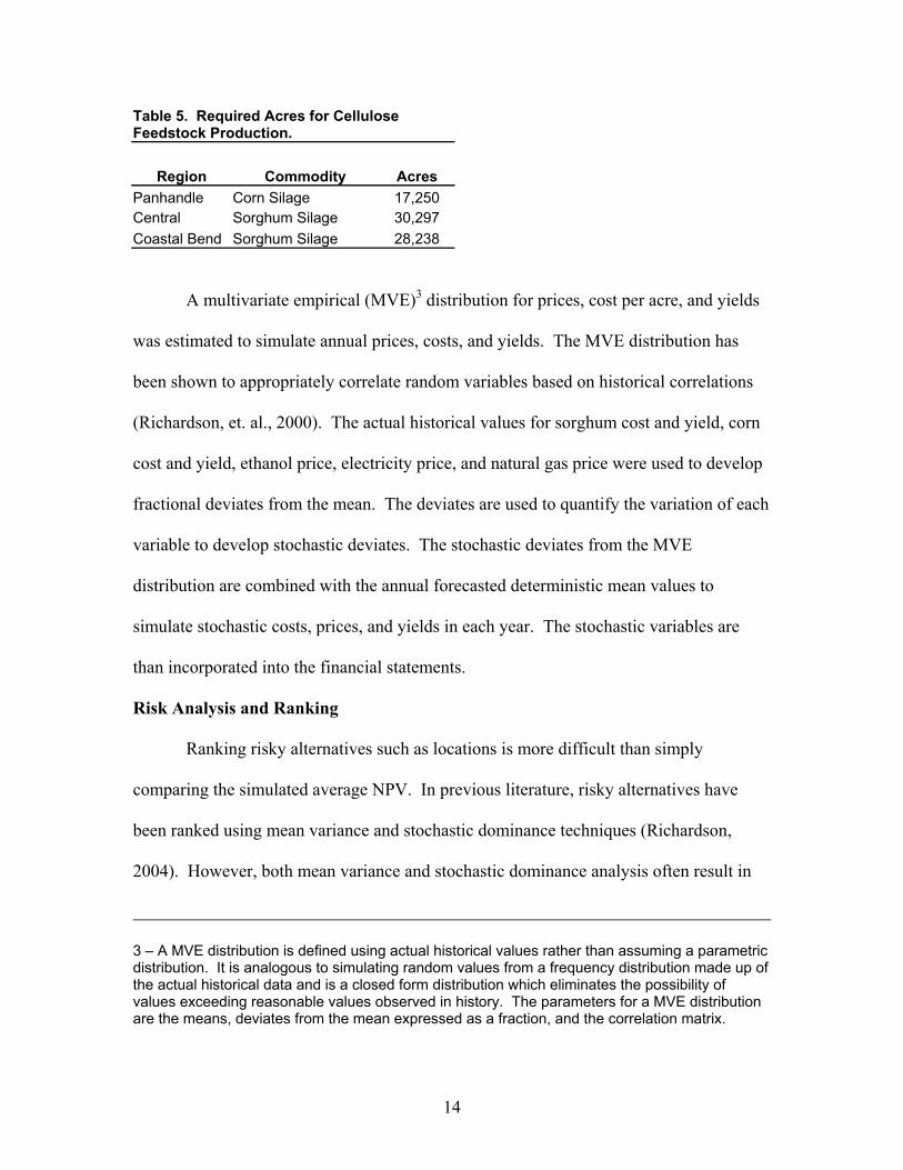
Table 5. Required Acres for Cellulose Feedstock Production.

Region Commodity Acres Panhandle Corn Silage 17,250 Central Sorghum Silage 30,297 Coastal Bend Sorghum Silage 28,238

A multivariate empirical (MVE)3 distribution for prices, cost per acre, and yields

was estimated to simulate annual prices, costs, and yields. The MVE distribution has

been shown to appropriately correlate random variables based on historical correlations

(Richardson, et. al., 2000). The actual historical values for sorghum cost and yield, corn

cost and yield, ethanol price, electricity price, and natural gas price were used to develop

fractional deviates from the mean. The deviates are used to quantify the variation of each

variable to develop stochastic deviates. The stochastic deviates from the MVE

distribution are combined with the annual forecasted deterministic mean values to

simulate stochastic costs, prices, and yields in each year. The stochastic variables are

than incorporated into the financial statements.

Risk Analysis and Ranking

Ranking risky alternatives such as locations is more difficult than simply

comparing the simulated average NPV. In previous literature, risky alternatives have

been ranked using mean variance and stochastic dominance techniques (Richardson,

2004). However, both mean variance and stochastic dominance analysis often result in

3 – A MVE distribution is defined using actual historical values rather than assuming a parametric distribution. It is analogous to simulating random values from a frequency distribution made up of the actual historical data and is a closed form distribution which eliminates the possibility of values exceeding reasonable values observed in history. The parameters for a MVE distribution are the means, deviates from the mean expressed as a fraction, and the correlation matrix.

15

inconclusive rankings for some types of decision makers (McCarl, 1988).

Stochastic efficiency with respect to a function (SERF) is a procedure for ranking

risky alternative scenarios when mean variance and stochastic dominance give

inconsistent results (Hardaker, et. al., 2004). SERF varies risk aversion over a defined

range and ranks risky alternatives in terms of certainty equivalence4. SERF can be used

with any utility function and can identify a smaller efficient set than stochastic

dominance analysis with respect to a function (SDRF). Using SERF will provide an

ordinal ranking of the three alternative location choices for the MixAlco facility within

feasible risk aversion boundaries. It will provide a cardinal measure for decision makers

based on risk preferences defined by the risk aversion coefficient (RAC5). Comparisons

between strongly risk adverse agents, risk neutral agents, and strongly risk-preferring

agents are possible with SERF.

RESULTS AND DISCUSSION

The simulated stochastic variables are compared to the historical values to

validate the simulation procedure. Statistical Student t-tests show all stochastic variables

were equal in mean, variance and correlation to the respective historical values at the 0.05

significance level. This validates that the simulated stochastic variables return the

4 – Certainty equivalence (CE) is the amount of money a decision maker would be willing to pay to gain a fair bet for a risky alternative versus a risk-free alternative with the same average return. The concept of CE, introduced by Freund (1956) and refined by Hardaker (1997), can be used for evaluating risky decisions. 5 – RAC or r(x) is defined as a function of wealth (x) as the negative ratio of the second and first derivatives of a utility function u(x), where r(x) = -u’’(x)/u’(x) (Pratt, 1964; Arrow, 1965). The RAC is positive for risk aversion and diminishes for x if there is diminishing risk aversion (Hardaker et al., 1997). The RACs represent the decisions maker’s degree of risk aversion (RAC>0), neutrality (RAC=0), and preference (RAC<0) and are used to classify decisions makers. SERF ranks risky strategies over a feasible range of RACs and avoids having to estimate RACS for individual decision makers. Meyer (1997) suggests using a range of RACs so that ranking of risky alternatives could be made for policy applications.

16

given mean, variability, and maintain the appropriate correlation among variables.

Simulated corn silage yields in the Panhandle Region are higher than sorghum

silage yields in the Central and Coastal Bend Regions. However, average sorghum silage

yield is higher in the Coastal Bend Region than the Central Region but are not

statistically different at the 0.05 significance level using a Student t test. The similar

yields can be explained by the use of dry-land farming in both regions. The mean and

variance for the simulated yields in each region are statistically equal to their respective

historical values. The mean and variance of simulated values for prices and costs are

statistically equal in mean and variance to their respective historical values. The relative

risk, measured by the coefficient of variation (CV), is also equal. The average cost of

cellulose feedstock is highest in the Panhandle Region and lowest in the Coastal Bend

Region. Transportation cost for feedstock is highest in the Coastal Bend Region and

lowest in the Panhandle Region. All other variable costs were the same for each region.

The correlation matrix of simulated annual values for all stochastic variables was

tested against the historical correlation matrix. Tests show the difference between the

simulated correlation matrix and historical correlation matrix is not statistically

significant at the 0.01 significance level. Therefore, we can say the simulation model

reproduced the historical correlation among all stochastic variables.

Non-stochastic Results

Based on a mean (risk free) NPV ranking of the three alternative locations, the

location with the highest NPV is preferred. The deterministic NPVs are $3.7 million,

$25.1 million, and $25.8 million for the Panhandle, Central, and Coastal Bend Regions,

respectively. The Panhandle Region is the clearly the lowest while the Central and

17

Coastal Bend Regions are nearly identical. A decision maker cannot say the Central

Region is strongly preferred to the Coastal Bend Region and vice-versa.

Stochastic Results

The simulated NPVs for each region are presented as cumulative distribution

functions (CDFs) in Figure 2. The CDF graphs show the probability of NPV being less

than a particular value. Probability is measured on the vertical axis and values for NPV

are measured on the horizontal axis. The Central and Coastal Bend Regions showed a

zero probability of NPV being below zero. The Panhandle Region showed a slight

probability, 3 percent, that NPV will be below zero.

In this analysis, the Central Region returns the highest NPV at each probability

level (CDF line farthest to the right in Figure 2). Because the CDF graphs do not cross,

one can say risk-adverse, risk-neutral, and risk-preferring decision makers’ all prefer the

Central Region to the Panhandle and Coastal Bend Regions.

0

0.1

0.2

0.3

0.4

0.5

0.6

0.7

0.8

0.9

1

-5,000,000 5,000,000 15,000,000 25,000,000 35,000,000 45,000,000 55,000,000 65,000,000

Pro

babi

lity

Panhandle Central Coastal Bend

Figure 2. Cumulative Distribution Functions of NPV for a MixAlco Plant in Panhandle, Central, and Coastal Bend Regions of Texas.

18

Table 6 presents the minimum, mean, maximum, CV, and range for NPV in each

region. Table 8 shows values from the financial statements for each region. The

Panhandle Region has minimum, mean, and maximum NPVs of $-3.49 million, $6.7

million, and $17.36 million, respectively. These NPVs are all lower than the minimum,

mean, and maximum for the Central and Coastal Bend Regions. The Central Region

returned simulated NPVs of $15.73 million, $35.69 million, and $61.11 million for the

minimum, mean, and maximum. The Coastal Bend Region has minimum, mean, and

maximum NPVs of $13.2 million, $30.98 million, and $52.81 million. The Panhandle

Region had the lowest range while the Central Region had the highest range of all three

regions. The simulated relative risk is comparable in Central and Coastal Bend Regions.

The relative risk is higher in the Panhandle Region because there is greater variability in

the cost and yield per acre of corn silage.

Table 6. Minimum, Mean, Maximum, CV, and Range Values of Net Present Value for Panhandle, Central, and Coastal Bend Regions. In Millions of Dollars

Region Minimum Mean Maximum Range CV Panhandle -3.49 6.70 17.36 20.85 51.01 Central 15.73 35.69 61.11 45.38 22.97 Coastal Bend 13.20 30.98 52.81 39.61 22.78

The CDF graphs and simulation results in Table 6 clearly show the Central

Region is preferred over the Panhandle and Coastal Bend Regions. The difference in

NPV between the Panhandle Region versus the Central and Coastal Bend Regions can be

explained by the cost of cellulose feedstock. Even though corn silage yields cellulose

material more than sorghum silage per acre, the additional yield is not enough to

overcome the additional cost of corn silage. Cellulose feedstock cost is approximately 30

percent of all variable costs for the MixAlco Plant.

19

Feedstock costs per acre and yields are similar for the Central and Coastal Bend

Regions. The difference in NPV between the two regions is due to the increased cost of

transporting cellulose feedstock in the Coastal Bend Region. The Coastal Bend Region

requires a half ring area to supply the necessary feedstock because of the adjacent

coastline, thus increasing the travel distance and the average shipping cost per ton.

Figure 3 presents the SERF ranking for the three alternative locations. The SERF

results for comparing the Panhandle, Central, and Coastal Bend Regions reaffirms the

Central Region is preferred by all classes of decision makers because the certainty

equivalence (CE) line for the Central Region is above the CE lines for the Central and

Coastal Bend Regions for RAC levels6 of -0.000001 to +0.000001, indicating a

preference for the Central Region for all classes of decision makers.

0.00

10,000,000.00

20,000,000.00

30,000,000.00

40,000,000.00

50,000,000.00

60,000,000.00

-0.000001 -0.0000008 -0.0000006 -0.0000004 -0.0000002 0 0.0000002 0.0000004 0.0000006 0.0000008 0.000001

RAC

Panhandle Central Coastal Bend

Figure 3. Stochastic Efficiency with Respect to a Function Ranking of NPV for a MixAlco Plant in the Panhandle, Central, and Coastal Bend Regions of Texas.

20

Table 7 presents the calculated risk premiums between the locations. The

absolute differences between the CE lines in Figure 3 represent the risk premium decision

makers place on the preferred alternative over another alternative. Risk premiums

represent the amount of money decision makers would have to be paid to be indifferent

between two risky alternatives

Table 7. Risk Premiums between Panhandle, Central, and Coastal Bend Regions Assuming Alternative Classes of Risk Preferences.* In Millions of Dollars Region Risk-Loving Risk-Neutral Risk-Averse Panhandle -43.42 -29.00 -19.74 Coastal Bend -8.25 -4.71 -2.35 * The Central Region is used as the base location for comparison.

The Central Region is used as the base region for comparison to calculate the risk

premiums. Risk-loving decision makers have risk premiums of $43.42 million and $8.25

million when comparing the Central Region to the Panhandle Region and Coastal Bend

Region. The risk premiums for risk-neutral decision makers are $29 million and $4.71

million for the Central Region compared to the Panhandle and Coastal Bend Regions.

Risk-averse decision makers have the smallest risk premiums, $19.74 million and $2.35

million for the same comparisons, respectively. A decision maker would have to be paid

these amounts to be indifferent from locating in the Central Region to the Panhandle

Region or from the Central Region to the Coastal Bend Region. These results are

consistent for entire range of risk aversion levels. Because the risk premiums are so

large, we are more confident that the ranking is robust (Mjelde and Cochran, 1988).

6 – Ranges of -0.000001 to 0.000001 were used for RAC values to demonstrate the ranking of alternative locations across a wide range of decision makers. If the rankings change over the given RAC range, then alternative locations can be preferred at different risk aversion levels.

21

SUMMARY AND CONCLUSIONS

The fuel oxygenate market has grown at a rapid pace due to increasing gasoline

prices and federal legislation mandating a reduction in air pollution. Because MTBE is

being banned for water pollution and ethanol production is costly, MixAlco was

developed as an alternative process of for making alcohol fuel for oxygenation. Because

any biomass source can be used as feedstock for conversion to alcohol fuel, a number of

location choices for MixAlco production is possible.

Location choices greatly affect the economic success of a business. Regional

differences in the cost of land, input costs, available inputs, and transportation costs, all

add risk when evaluating alternative locations. The objective of this study is to compare

three alternative locations in Texas for a MixAlco production facility under a

probabilistic framework. The method used in this study for decision-making under risk is

to estimate the distribution for each alternative locations’ NPV using simulation. Each

location is than ranked based on the characteristics of the simulated NPV distribution

using the SERF risk ranking procedure.

Based on the non-stochastic NPV ranking, the Panhandle Region is the least

preferred location while the Central and Coastal Bend Regions returned almost identical

NPVs. A decision maker cannot say Central Region is preferred to the Coastal Bend

Region and vice-versa. Results of simulating the alternative locations under risk were

presented as CDFs of NPV. Since the NPVs do not cross, one can say that the Central

Region is preferred over the other two regions for all classes of decision makers. SERF

rankings show the Central Region is preferred to the Panhandle and Coastal Bend

Regions for risk-loving, risk-neutral, and risk-adverse decision makers.

22

Risk premiums range from $43.42 million for risk-loving decision makers to

$19.74 million for risk-adverse decisions makers when comparing the Central Region to

the Panhandle Region. Risk premiums when comparing the Central Region to the

Coastal Bend Region for risk-loving decision makers are $8.25 million and $2.35 million

for risk-adverse decision makers.

The results of this study provide useful information to compare the risk and

benefits of MixAlco production. If the alcohol fuel is priced similar to ethanol, MixAlco

production can be profitable and could substantially impact the fuel oxygenate market.

The ability of MixAlco to convert any biomass material to alcohol fuel makes it an

attractive alternative to ethanol production. Large amounts of available residual biomass

represent a low cost feedstock source that can be used on MixAlco production. However,

even in the Panhandle Region where feedstock cost was highest, MixAlco production

returned a 97 percent probability that NPV will be positive.

LIMITATIONS OF THE STUDY

Historical budgets for the three regions are limited from 1998 to 2003.

Alcohol yield is constant for this analysis but may vary in real life production. Lab

experiments have shown yield may vary from the mean 93 gallons/ton feedstock.

No MixAlco facility is in production. The initial capital investment of $20.1 million

is only an estimate and may increase with the uncertainties of new technology.

This study is limited to three locations and production of feedstock for fuel

conversion. Alternative locations and residual biomass may be available.

No location incentives were considered in this study.

23

REFERENCES

Agriculture and Food Policy Center. “Represented Farm Project.” Texas A&M University, College Station, TX, 2004.

Arrow, K.J. Aspects of the Theory of Risk-Bearing. Academic Bookstore, Helsinki,

Findaland, 1965. Australian CRC for Renewable Energy Ltd. “What is Biomass?.”

<http://acre.murdoch.edu.au/refiles/biomass/text.html> Badger, P.C. "Ethanol from Cellulose: A General Review." Trends in New Crops and

Uses, 2002. Bassam, N. “Global Potential of Biomass for Transport Fuel.” Federal Agriculture

Research Center, Institute of Crop and Grassland Science. California Energy Commission. “Evaluation of Biomass-to-Ethanol Fuel Potential in

California.” Publication P550-99-011. <http://energy.ca.gov/mtbe/ethanol/1999-08-16_500-99-011.html> 1999.

Energy Information Administration, U.S. Department of Energy,

<http://www.eia.doe.gov/> 2004. Gallagher, P. W., M. Dikeman, J. Fritz, E. Wailese, W. Gauther, and H. Shapouri.

“Biomass from Crop Residues, Cost and Supply Estimates.” Office of Energy Policy and New Uses. AER-819.

Greenhut, M.L. A Theory of the Firm in Economic Space. Austin Press, Educational

Division, Lone Star Publishers, Inc., 1974. Hardaker, J.B., Huirne, R.B.M., and J.R. Anderson. Coping with Risk in Agriculture.

Chapter 7, 1997. Hardaker, J.B., J. W. Richardson, G. Lien, and K. D. Schumann. “Stochastic Efficiency

Analysis with Risk Aversion Bounds: A Simplified Approach.” Australian Journal of Agriculture and Resource Economics, Forthcoming, 2004.

Hart’s Oxy-Fuel News, 2003. Herbst, B. K. “The Feasibility of Ethanol Production in Texas.” M.S. Thesis, Department

of Agriculture Economics, Texas A&M University, 2003. Holtzapple, M. “MixAlco Process.” Texas A&M University, College Station, TX, 2003.

24

Isik, M., K. H. Coble, D. Hudson, and L. O. House. A Model of Entry-Exit Decisions and Capacity Choice under Demand Uncertainty. Unpublished manuscript presented at the 2002 American Agriculture Economics Association Annual Meeting, July, 2002.

Mazza, P. "Ethanol: Fueling Rural Economic Revival." Climate Solutions Report. McCarl, B. “Preference Among Risky Prospects Under Constant Risk Aversion.” Journal

of Agriculture and Applied Economics 20:25-33, Dec. 1988. Meyer, J. “Choice Among Distributions.” Econometric Theory 14:326-336, 1997. Mjelde, J.W. and M.J. Cochran. “Obtaining Lower and Upper Bounds on the Value of

Seasonal Climate Forecasts as a Function of Risk Preferences.” Western Journal Agriculture Economics 13:285-293, Dec. 1988.

National Agriculture Statistics Service, U.S. Department of Agriculture,

<http://www.usda.gov/nass/> 2004. Office of Industrial Technology. Biobased Products: Chemicals and Materials.

Unpublished manuscript presented at the 2001 Bioenergy Feedstock Meeting, November 2001.

Pouliquen, L.Y. Risk Analysis in project Appraisal. Baltimore, MD: The Johns Hopkins

University Press, 1970. Pratt, J.W. “Risk Aversion in the Small and in the Large.” Econometrica 32: 122-136,

1964. Renewable Fuels Association. “Ethanol Industry Outlook 2003.” 2003. Reutlinger, S. Techniques for Project Appraisal Under Risk. Baltimore: The John

Hopkins Press, 1970. Richardson, J.W., K. Schumann, and P. Feldman. Simulation for Applied Risk

Management. Department of Agriculture Economics, Texas A&M University. 2004. Richardson, J.W. and H.P. Mapp, Jr. “Use of Probabilistic Cash Flows in Analyzing

Investment Under Conditions of Risk and Uncertainty.” Journal of Agriculture and Applied Economics 8:19-24, Dec. 1976.

Richardson, J.W., S.L. Klose, and A.W. Gray. "An Applied Procedure for Estimating and

Simulating Multivariate Empirical (MVE) Probability Distributions in Farm Level Risk Assessment and Policy Analysis." Journal of Agriculture and Applied Economics 32,2:299-315, Aug. 2000.

25

Shapouri, H. The U.S. Biofuel Industry: Present and Future. Unpublished manuscript presented at the 2003 Conference Agro-Demain, December 2003.

So, K. S., P. F. Orazem, and D. M. Otto, The Effects of Housing Prices, Wages, and

Commuting Time on Joint Residential and Job Location Choices. Unpublished Manuscript presented at the 1998 American Agriculture Economics Association Annual Meeting, July 1998.

Sterling Planet. “Energy for Biomass.” <http://sterlingplanet.com/sp/biomass.jsp> Texas Extension Agriculture Economics. “Texas Crop and Livestock Budgets.”

<http://agecoext.tamu.edu/> 2004. Texas Agriculture Statistics Service. 1999 Texas Custom Rates Statistics. Texas

Agriculture Extension Service, 1999. Veringa, H.J. "Advanced Techniques for Generation of Energy from Biomass and

Waste.” ECN Biomass.

26

Tabl

e 8.

Sim

ulat

ed M

ean

Valu

es fr

om th

e Fi

nanc

ial S

tate

men

ts fo

r a M

ixA

lco

Plan

t in

the

Panh

andl

e, C

entr

al, a

nd C

oast

al B

end

Reg

ions

of T

exas

.

In

Mill

ions

of D

olla

rs

Panh

andl

e R

egio

n 20

04

2005

20

06

2007

20

08

2009

20

10

2011

20

12

2013

20

14

2015

20

16

2017

20

18

Gro

ss In

com

e 17

.91

35.8

335

.86

35.8

936

.00

36.1

036

.27

36.2

6 36

.37

36.4

436

.50

36.5

036

.50

36.4

136

.47

Tot

al C

ost*

15

.27

28.8

729

.38

29.9

530

.43

30.9

731

.52

32.0

6 32

.66

33.2

233

.82

34.4

335

.02

35.6

036

.24

Net

Inco

me

(Los

s)

2.64

6.

96

6.48

5.

94

5.57

5.

13

4.76

4.

20

3.71

3.

22

2.68

2.

07

1.47

0.

81

0.23

E

ndin

g C

ash

Bal

ance

1.

52

5.00

8.

23

11.1

813

.91

16.4

118

.68

20.6

3 22

.30

23.6

424

.61

25.1

325

.18

24.7

323

.73

Tot

al A

sset

s 20

.96

23.7

726

.33

28.6

130

.68

32.5

034

.10

35.3

8 36

.39

37.0

537

.35

37.2

136

.59

35.4

633

.79

End

ing

Net

Wor

th

11.2

7 14

.49

17.4

820

.22

22.7

925

.16

27.3

529

.27

30.9

532

.36

33.4

634

.18

34.4

934

.37

33.7

9 D

ivid

ends

Pai

d 0.

52

1.38

1.

28

1.18

1.

10

1.02

0.

94

0.84

0.

74

0.67

0.

58

0.50

0.

43

0.34

0.

30

C

entr

al R

egio

n 20

04

2005

20

06

2007

20

08

2009

20

10

2011

20

12

2013

20

14

2015

20

16

2017

20

18

Gro

ss In

com

e 18

.10

36.0

936

.34

36.2

936

.61

36.8

737

.07

37.2

8 37

.36

37.5

937

.86

38.0

738

.17

38.1

138

.37

Tot

al C

ost*

12

.59

23.3

723

.75

24.1

024

.58

25.0

525

.41

25.8

9 26

.29

26.7

627

.22

27.7

528

.17

28.6

029

.10

Net

Inco

me

(Los

s)

5.51

12

.72

12.5

912

.19

12.0

211

.82

11.6

611

.39

11.0

710

.83

10.6

310

.32

10.0

09.

51

9.27

E

ndin

g C

ash

Bal

ance

2.

85

9.72

16

.55

23.0

329

.43

35.6

041

.68

47.6

2 53

.24

58.6

863

.96

69.0

773

.85

78.1

882

.37

Tot

al A

sset

s 22

.30

28.5

034

.66

40.4

746

.20

51.7

057

.11

62.3

8 67

.33

72.1

076

.71

81.1

585

.26

88.9

292

.44

End

ing

Net

Wor

th

12.6

1 19

.21

25.8

032

.08

38.3

144

.36

50.3

656

.26

61.9

067

.41

72.8

278

.12

83.1

687

.83

92.4

4 D

ivid

ends

Pai

d 1.

09

2.83

2.

83

2.69

2.

67

2.59

2.

57

2.53

2.

42

2.36

2.

32

2.27

2.

16

2.00

1.

97

C

oast

al B

end

Reg

ion

2004

20

05

2006

20

07

2008

20

09

2010

20

11

2012

20

13

2014

20

15

2016

20

17

2018

G

ross

Inco

me

17.9

6 35

.95

36.1

236

.18

36.4

136

.61

36.9

137

.05

37.1

537

.32

37.5

037

.62

37.7

337

.77

37.9

7 T

otal

Cos

t*

12.7

9 23

.99

24.3

924

.80

25.2

525

.68

26.1

526

.58

27.0

227

.52

27.9

928

.41

28.9

629

.39

29.9

1 N

et In

com

e (L

oss)

5.

17

11.9

611

.73

11.3

811

.16

10.9

210

.76

10.4

8 10

.13

9.80

9.

51

9.21

8.

77

8.38

8.

06

End

ing

Cas

h B

alan

ce

2.69

9.

03

15.2

721

.19

26.9

832

.60

38.0

943

.33

48.3

753

.19

57.6

461

.91

65.9

469

.56

72.9

7 T

otal

Ass

ets

22.1

4 27

.81

33.3

838

.63

43.7

548

.70

53.5

258

.09

62.4

666

.61

70.3

973

.99

77.3

580

.30

83.0

4 E

ndin

g N

et W

orth

12

.45

18.5

224

.52

30.2

435

.86

41.3

646

.77

51.9

7 57

.02

61.9

166

.50

70.9

675

.25

79.2

283

.04

Div

iden

ds P

aid

1.02

2.

60

2.57

2.

45

2.41

2.

36

2.32

2.

23

2.17

2.

10

1.97

1.

92

1.84

1.

71

1.65

* I

nclu

des

depr

ecia

tion

cost

.