LODOP – Multi-Query Optimizationfor Linked Data Profiling Queries

Benedikt Forchhammer1, Anja Jentzsch1, and Felix Naumann1

Hasso-Plattner-Institute firstname.lastname@hpi.uni-potsdam.de

Abstract. The Web of Data contains a large number of different, openly-available datasets. In order to effectively integrate them into existingapplications, meta information on statistical and structural propertiesis needed. Examples include information about cardinalities, value pat-terns, or co-occurring properties. For Linked Datasets such informationis currently very limited or not available at all. Data profiling techniquesare needed to compute respective statistics and meta information. How-ever, current state of the art approaches can either not be applied toLinked Data, or exhibit considerable performance problems.

We present Lodop, a framework for computing, optimizing, and bench-marking data profiling techniques based on MapReduce with ApachePig. We implemented 15 of the most important data profiling tasks, opti-mized their simultaneous execution, and evaluate them with four typicaldatasets from the Web of Data. Our optimizations focus on reducing theamount of MapReduce jobs and minimizing the communication overheadbetween multiple jobs. Our evaluation shows the significant potential inoptimizing the runtime costs for Linked Data profiling.

1 Introduction

Over the past years, an increasingly large number of datasets has been publishedas part of the Web of Data. This trend, together with the inherent heterogeneityof datasets and their schemata, makes it increasingly time-consuming to findand understand datasets that are relevant for integration. In order for users tobe able to integrate Linked Data, they first need an easy way to discover andunderstand relevant datasets on the Web of Data.

Data profiling is an umbrella term for methods that compute meta-data fordescribing datasets [1]. Traditional data profiling tools for relational databaseshave a wide range of features ranging from the computation of cardinalities,such as the number of values or distinct values in a column, to the calculationof inclusion dependencies between multiple columns or sets of columns; theycalculate histograms on numeric values, determine value patterns, and gatherinformation on used data types; some tools also determine the uniqueness ofcolumn values, and find and validate keys and foreign keys.

Use cases for data profiling can be found in various areas concerned withdata processing and data management [1].

Query optimization is concerned with finding optimal execution plans fordatabase queries. Cardinalities and value histograms can help to estimate thecosts of such execution plans. Such metadata can also be used in the area ofLinked Data, e.g., for optimizing SPARQL queries.

Data cleansing can benefit from discovered value patterns. Violations of de-tected patterns can reveal data errors, and respective statistics help measureand monitor the quality of a dataset. For Linked Data, data profiling techniqueshelp validate datasets against vocabularies and schema properties, such as valuerange restrictions.

Data integration is often hindered by the lack of information on new datasets.Data profiling metrics reveal information on, e.g., size, schema, semantics, anddependencies of unknown datasets. This is a highly relevant use case for LinkedData, because for many openly available datasets only little information is avail-able1.

Schema induction: Raw data, e.g., data gathered during scientific experiments,often does not have a known schema at first; data profiling techniques need todetermine adequate schemata, which are required before data can be insertedinto a traditional DBMS. For the field of Linked Data, this applies when workingwith datasets that have no dereferencable vocabulary. Data profiling can helpinduce a schema from the data, which then can be used to find a matchingexisting vocabulary or create a new one.

The process of running data profiling tasks for large Linked Datasets can takehours to days, depending on the complexity of task and the size of the respectivedatasets. Data set characteristics highly influence the profiling task runtime. Asan example, our Property Cooccurrence by Resource script (see Sec. 3) runs 16hours for only 1 million triples of the Web Data Commons RDFa dataset incontrast to 5 min on Freebase and 9 min on DBpedia.

We have compiled a list of 56 data profiling tasks implemented in ApachePig to be executed on Apache Hadoop. At this point Apache Pig only appliessome basic logical optimization rules, like removing unused statements [2]. Wepresent Lodop, a framework for executing, optimizing, and benchmarking sucha set of profiling tasks, highlight reasons for poor performance when executingthe scripts sequentially, and develop a number of optimization techniques. Inparticular, we developed and evaluated three multi-script optimization rules forcombining logical operators in the execution plans of profiling scripts.

2 Related Work

While many tools and algorithms already exist for data profiling in general, mostof them can, unfortunately, not be used for graph datasets, because they assumea relational data structure, a defined schema, or simply cannot deal with verylarge datasets. Nonetheless, some Linked Data profiling tools already exist. Mostof them focus on solving specific use cases instead of data profiling in general.

1 http://lod-cloud.net/state/#data-set-level-metadata

One relevant use case is schema induction, because not having a fixed andwell-defined schema is a common problem with Linked Datasets. One examplefor this field of research is the ExpLOD tool [3]. ExpLOD creates summaries forRDF graphs based on class and predicate usage. It can also help understand theamount of interlinking between datasets based on the owl:sameAs predicate. Lidescribes a tool that can induce the actual schema of an RDF dataset [4]. Itgathers schema-relevant statistics like cardinalities for class and property usage,and presents the induced schema in a UML-based visualization. Its implemen-tation is based on the execution of SPARQL queries against a local database.Like ExpLOD, the approach is not parallelized in any way. It is evaluated withdifferent datasets of up to 13M triples and reportedly faster than ExpLOD.However, both solutions still take approximately 10h to process a 10M triplesdataset with 13 classes and 90 properties. These results illustrate performanceas a common problem with large RDF datasets, and indicate that there is a needfor parallelized, distributed execution.

An example for the query optimization use case is presented in [5]. Theauthors present RDFStats, which uses Jena’s SPARQL processor for collectingstatistics on RDF datasets. These include histograms for subjects (URIs, blanknodes) and histograms for properties and associated ranges. These statistics areused to optimize query execution on the (discontinued) Semantic Web Integratorand Query Engine. Others have worked more generally on generating statisticsthat describe datasets on the Web of Data and thereby help understandingthem. LODStats computes statistical information for datasets from The DataHub2 [6]. It calculates 32 simple statistical criteria, e.g., cardinalities for differentschema elements and types of literal values (e.g., languages, value data types).Approximation techniques are used when memory limits are reached. No detailedinformation about the performance of LODStats is reported.

In [7] the authors use MapReduce to automatically create VoID descriptionsfor large datasets. They manage to profile the Billion Triple Challenge 2010dataset in about an hour on Amazon’s EC2 cloud, showing that parallelizationcan be an effective approach to improve runtime when profiling large amountsof data. Finally, the ProLOD++ tool allows to navigate an RDF dataset viaan automatically computed hierarchical clustering [8] and along its ontology [9].Data profiling tasks are performed on each cluster independently, which servesnot only as a means to derive meaningful results, but also improves efficiency.

3 Linked Data Profiling Tasks

This section lists and explains a set of useful data profiling tasks to profileLinked Data sets. We have implemented a total of 56 data profiling scripts,which compute 15 different statistical properties across different subsets of theinput dataset. These subsets are determined via the following types of groupings:

Overall: no grouping.

2 http://datahub.io

Resource: grouping based on the triple subject; usually paired with some top-klist of resources.

Property: grouping based on the property type.

Class: grouping based on the value of the rdfs:type predicate on a resource.

Class & Property: grouping based on both class and property type.

Datatype: grouping based on the (declared) data type of the object value; onlytyped literals are considered.

Language: grouping based on the (declared) language of the object value; onlylanguage literals are considered.

Context URL: grouping based on the N-Quads context attribute. Values beingaggregated based on the context URL are grouped three times: based on the fullURL, the pay-level-domain (PLD) part of the URL, and the top-level-domain(TLD) part of the UR.

Vocabulary: grouping based on the vocabularies used for predicates or classes.

Object URI: grouping based on the value of the object. Only URI values areconsidered.

The following data profiling tasks are computed. Unless stated differently, ex-amples have been generated from a 1 million triples subset of DBpedia. Moreinformation on datasets can be found in Section 6.

Number of triples for each of the following groupings: overall, resource, prop-erty, object URI, context URL. This highlights, e.g., that the largest resources inour DBpedia subset is http://dbpedia.org/resource/2010-11_SC_Freiburg_season with 867 triples, and the most used property type is rdfs:type with86,856 triples. (7 scripts)

Average number of triples per resource within each of the following group-ings: overall, context URL, class. This reveals that resources in our DBpediasubset are made up of 5.9 triples on average, and that some classes, such ashttp://dbpedia.org/ontology/YearInSpaceflight, have resources with anaverage number of 502 triples. (5 scripts)

Average number of triples per object URI highlights how often certainURI objects are used across the dataset. For our DBpedia subset, each URIobject is (re-)used as the object value for an average of 2.6 triples. For our1 million triples subset of Freebase, this number is lower (1.9), i.e., fewer URIobject values are reused. (1 script)

Average number of triples per URL computes the average number of triplesper value of the graph context URL. For our DBpedia subset, each graph con-text contains an average of 47.8 triples. This means that, in this case, multipleresources share the same graph context, because the average number of triplesper resource is only 5.9 as mentioned above. (1 script)

Number of property types within each of the following groupings: overall,context URL, resource, class, data type. This tasks tells us how many propertytypes are used in different contexts; our DBpedia subset has a total of 7,844

different property types, of which 4,970 are used on resources of the class owl:

Thing. It also reveals that 2,929 property types point to triples having typedobject values with the xsd:int datatype. (7 scripts)

Average number of property values per property type (i.e., triples perpredicate) within each of the following groupings: overall, context-URL, resource,class, property, class, property. For example, resources having the class http://umbel.org/umbel/rc/Event have an average number of 115 values for the http://dbpedia.org/property/time predicate in our DBpedia subset. (8 scripts)

Number of resources in each of the following groupings: property, class,datatype, language, vocabulary. On our subset of DBpedia, these profiling taskstell us that there are a total of 169,035 resources, that the owl:sameAs propertytype is used on 43,840 resources, and the http://xmlns.com/foaf/0.1/Person

class on 4,140 resources. (6 scripts)

Number of context URLs in each of the following groupings: property, class,vocabulary. For DBpedia the context URL usually matches to the correspondingWikipedia page. This task can reveal how many Wikipedia pages lead to certainclasses; for example, the foaf:Person class occurs in 4,140 different contextURLs in our subset of data. (3 scripts)

Number of context PLDs in each of the following groupings: property, class,vocabulary. Alternative script versions additionally group by the TLD of thecontext URL. Similar to the previous task, this task can tell us how manydifferent pay-level domains are responsible for certain properties, classes, orvocabularies. For our WDC RDFa subset (1m triples) this reveals, e.g., thatthe http://www.facebook.com/2008/ predicate is used by 452 domains, whichmakes it the most-used property type in this subset. (6 scripts)

Property co-occurrence computes a list of pairs of property types that areused together: a) on the same resource (by resource), b) within the same con-text URL (by url), or c) pointing to the same resource (by object URI). Thisreveals patterns, such as http://dbpedia.org/ontology/artist and http:

//dbpedia.org/property/title being used together on resources describingartistic work. (3 scripts)

Inverse properties computes a list of properties that are inverse to each other.For example, the relationship between a musician and his band can be de-clared on both resources with two inverse property types http://dbpedia.org/ontology/associatedBand and http://dbpedia.org/ontology/bandMember.(1 script)

URI-literal ratio computes the ratio between the number of URI values andliterals within the following groupings: overall, class, context URL. Our DBpediasubset contains almost as many URI object values as it contains literal values(ratio 1.1); however, the RDFa subset contains far more literals than URI values(ratio 0.2). (5 scripts)

Property value ranges of literal values per property type (numeric and tem-poral values only). For example, the http://dbpedia.org/ontology/bedCountproperty has numeric values between 76 and 785 in our DBpedia subset. (2 scripts)

Average value length of literals per property type can reveal schema prop-erties. For example, the http://dbpedia.org/ontology/title property hasvalues with an average length of 34 characters, whereas values for the http:

//dbpedia.org/property/longTitle property have an average of 288 charac-ters. (1 script)

Number of inlinks computes the number of URI values pointing to otherresources within the same dataset/file. For DBpedia, there are 207,712 valuespointing to resources within the same dataset; for our WDC RDFa subset, thereare far fewer inlinks (35,329). (1 script)

Each of these profiling tasks have been implemented as an Apache Pig scriptand are availabe at https://github.com/bforchhammer/lodop. The runtimeof these scripts even on 1 million triples might take up to hours, e.g., for theproperty co-occurrence determination. Also, scripts often have the same pre-processing steps, e.g., filtering or grouping the dataset. Thus there is a largeincentive and potential to optimize the execution of multiple scripts.

4 Multi-query optimization for Apache Pig

A prevalent goal for relational database optimization is to reduce the amount ofrequired full table scans, which for file-based database systems effectively meansreducing the amount of disk operations. Sellis introduces Multi-Query Optimiza-tion for relational databases as the process of optimizing a set of queries whichmay share common data [10]. The goal is to execute these queries together andreduce the overall effort by executing similar parts only once. The optimizationprocess consists of two parts: identifying shared parts in multiple queries andfinding a globally optimal execution plan that avoids superfluous computation.

Apache Pig3 is a platform for performing large-scale data transformationson top of Apache Hadoop clusters. It provides a high-level language (called PigLatin) for specifying data transformations, e.g., selections, projections, joins,aggregations and sorting on datasets. Pig Latin scripts are compiled into a seriesof MapReduce tasks and executed on a cluster.

The main goals for our multi-query optimization rules for Pig are the fol-lowing two: First, we attempt to minimize the dataflow between operators. Inour evaluation (Sec. 6) we identified the dataflow between MapReduce jobs as areasonable indicator for the performance of Pig scripts, as it is closely related tothe amount of required HDFS operations. Second, we try to avoid performingidentical or similar operations multiple times. The idea behind this is to free upcluster resources for other tasks. All optimization rules presented in this section,are based on optimizing the logical plans of Pig scripts.

Three optimization rules have been implemented: Rule 1 merges identicaloperators in logical plans of different scripts, Rule 2 combines FILTER operators,and Rule 3 combines aggregations, i.e., FOREACH operators. Rule 1 is a prereq-uisite for the other two rules, which work on pairs of siblings operators, i.e.,

3 http://pig.apache.org/

operators that have the same parent operator in a respective logical plan. Forall optimization rules, it was important to make sure that their usage does notaffect the intended output of scripts.

Rule 1 – Merge identical operators: In order to better utilize cluster re-sources, it makes sense to submit jobs to Apache Hadoop in parallel. Lodopsupports this by merging logical plans of different scripts into a single largeplan. In our experiments, executing scripts in parallel as part of one large plancuts execution time down to 25-30% of the time required to execute scripts se-quentially. Once all plans have been merged together, it’s possible to also mergeidentical operators.For 52 of our Pig scripts, this reduces the number of operatorsfrom 365 to 267.

Rule 2 – Combine filters: FILTER operators reduce the amount of data thatneeds to be processed in later steps of the execution pipeline. This optimizationrule aims to avoid iterating over large sets multiple times. From our selection ofprofiling scripts, 25 scripts perform filtering operations on the full initial dataset.

First, we identify all suitable sibling filters, i.e., all FILTER operators that havethe same parent operator. Second, a combined filter is created and we attach it tothe same parent operator. This combined filter contains all boolean expressionsof existing filters concatenated via OR. The expression of the combined filteris cleaned up by transforming it into disjunctive normal form. Finally, we re-arrange all previous filters and move them after the combined filter.

Rule 3 – Combine aggregations: FOREACH operators can be used for pro-jections and aggregations. Some instances perform identical aggregations, butproject different properties. This can happen, e.g., if the aggregation itself isonly a preprocessing step to another aggregation. These operators are not ex-actly identical, so the rule for merging identical operators will not be able tomerge them. However, these cases can be optimized by separating the aggre-gation from the projection, i.e., performing the aggregation only once with allprojected columns, and then projecting the exact columns afterwards. For ourset of scripts, this rule can be applied in seven different cases and combines vary-ing numbers of FOREACH operators from the minimum of two to a maximum ofeleven siblings operators.

While our goal is to optimize the performance of profiling tasks, the opti-mization rules can be applied on any Pig script.

5 The LODOP System

Lodop comprises four major components. Figure 1 shows how they interactwith the Hadoop cluster. The Compiler is responsible for compiling Pig Latinscripts into Logical Plans and eventually into MapReduce jobs; the Optimisertakes care of optimizing logical plans; the ScriptRunner schedules and monitorsthe execution of jobs on the Hadoop cluster; finally, the Reporting componentturns raw statistics into human-readable formats.

Lodop is built to be easily configurable via command line arguments, allow-ing the execution of different combinations of datasets, scripts, and optimization

Fig. 1. LODOP component overview

rules. The benchmarking system parses the arguments supplied by the user, andpasses them on to the compiler. The main responsibility of the compiler is tomake sure that Apache Pig plays well with the optimization component. It takesover Pig’s standard script compilation workflow, and adds in missing features,such as the support for multiple scripts and custom optimization rules.

The compiler first loads the declared list of scripts and compiles them intorespective logical plans. This compilation step is largely taken care of by ApachePig’s compiler, which parses Pig Latin and builds a respective directed acyclicgraph of logical operations. Once these logical plans have been created, our stan-dardized loading and storage functions are injected into each plan. The loadingfunction assumes that all scripts work with the same input file type and schema(N-Quads files). This is an essential prerequisite for merging different scriptstogether in the optimization component. Similarly, outputs are also handled au-tomatically, by always storing the result of the last statement in each script.The respective storing function writes results directly to Hadoop’s distributedfile system (HDFS).

Rule-based optimization is now done in two steps: First, all existing logicalplans are merged into one large logical plan. At this point, each script’s logicaldata flow is still separate from other scripts, but this allows the ScriptRunnercomponent to submit jobs for different scripts at the same time, and thus executethem in parallel. Second, optimization rules are applied to the merged logicalplan. The rules function similar to other optimization rules that are already partof Pig: First the logical plan is searched for applicable patterns in order to gaina list of possible optimization targets. Each match is then checked to determine

whether the rule can be applied to the specific group of operators. Finally, if allchecks are positive, the rule is applied and the logical plan adjusted accordingly.

Lodop currently does not perform cost-based optimization to determinewhether a rule should be applied or not; we simply apply rules repeatedly un-til they cannot be applied any more. To ease debugging and help understandlogical plans, the system additionally visualizes plans after different steps in thecompilation and optimization process.

After the optimization step, logical plans are compiled into MapReduce plansand then handed to the ScriptRunner component. The ScriptRunner submitsMapReduce jobs to the Hadoop cluster, monitors their execution, and gathersperformance statistics. Scheduling and monitoring are handled by Apache Pigitself. Statistics on the performance of MapReduce jobs are provided by Hadoopand only need to be retrieved from the cluster.

6 Evaluation

In this section we evaluate the effect of applying the optimization rules of Sec. 4and investigate under which circumstances the performance is improved. Weevaluate on four selected Linked Data sets that provide a wide range of charac-teristics, ranging from cross-domain to domain-specific as well as ranging fromwell-defined to loosely defined semantics.

6.1 Datasets and experimental setup

DBpedia4 is one of the largest Linked Data sets and contains structured infor-mation extracted from Wikipedia. As such it covers a wide range of differenttopics with a large number of property types and a very large number of classescompared to other datasets. Almost 50% of property values are URIs.

Freebase5 is a community-maintained database of “well-known people, places,and things”. It contains data harvested from sources such as Wikipedia, Chef-Moz, MusicBrainz, and others. It has a fairly small average number of triplesper resource (4.4), but the highest number of URI values.

The Web Data Commons6 project extracts RDF triples directly from infor-mation embedded on websites via RDFa, Microdata, or Microformats. We focuson only the RDFa subset (roughly 500 million triples) which is mostly unstruc-tured and has a small schema compared to other datasets. Most property valuesare literal values (83%) and there are very few in-links (3%). Any faulty defi-nitions on crawled websites can lead to inconsistencies and errors in the triplegraph, e.g., resources that do not conform to well-known schema definitions.

The species dataset of the European Environment Agency (EUNIS)7 is partof a database on species, habitat types, and sites of interest for biodiversity.

4 http://dbpedia.org5 http://www.freebase.com6 http://webdatacommons.org7 http://eunis.eea.europa.eu

The species subset is well-structured with only one class and 16 property types.Compared to other datasets it has a very large average number of triples perresource (15.2).

All evaluations were performed on an Apache Hadoop cluster with one headnode and ten slaves. Each node has a 2-core processor (Core 2 Duo) with 2GBof memory and runs CentOS 5.5. We use Apache Hadoop 1.1.2 and Apache Pig0.11.1 with Java 1.7. In order to explain our observations, we particularly look atthe properties identified as relevant to performance, i.e., the number of operatorsand MapReduce jobs, as well as the amount of I/O activity on HDFS.

6.2 Base performance analysis

This section analyzes the overall runtime of scripts, when executed without anycustom optimizations. We thus establish a baseline against which our customoptimization rules can be compared, and give insights into the reasons for currentperformance.

Figure 2 shows an overview of execution times for all scripts executed on 1million triples of DBpedia, Freebase, WDC RDFa, and EUNIS. The figure showsthat execution times vary depending on the dataset and the script. Overall, onecan see that many scripts finish in under 5 minutes. Some scripts have to performmore complex computations and hence take longer to complete. This includesthe scripts for computing property co-occurrence and the URI-Literal ratio byClass script. These UDF-based scripts dominate the overall execution time, arenot amenable to our rules, and are thus excluded from further evaluation.

Fig. 2. Runtime overview for all datasets (1M triples)

6.3 Effectiveness of merging identical operators

As described in Section 5, Lodop supports two ways for executing multiplescripts: First, they can simply be loaded, compiled, and executed sequentially.

In this case, the monitoring and scheduling overhead of Apache Pig takes someadditional time between jobs and also between scripts, during which the clusteris idle. In order to better utilize cluster resources, it makes sense to submit jobsto Apache Hadoop in parallel instead. Lodop supports this by merging logicalplans of different scripts together into one large plan. By executing multiplejobs simultaneously, Apache Pig can start a MapReduce job, as soon as all itsdependent jobs have finished. Figure 3 shows that this has a large impact on theoverall runtime of the profiling process, cutting execution time down to 25-30%of the execution time required to execute scripts sequentially.

Fig. 3. Execution time for 52 scripts, sequential execution versus merged plan execution

Once all plans have been merged, it is possible to apply the first optimiza-tion rule, merge identical operators. For 52 scripts, this reduces the number ofoperators from 365 to 267. Table 1 shows that we are able to merge, amongstothers, 14 COGROUPs, 12 FOREACHs and 1 JOIN into respective identical operators.In terms of MapReduce jobs, merging identical operators reduces the number ofjobs from 176 jobs to 140.

Pig Operator Defined in scripts Identical operators merged

COGROUP 66 52

ORDER BY 44 44

STORE 52 52

JOIN 6 5

DISTINCT 15 11

FOREACH 98 86

FILTER 28 13

LOAD 52 1

UNION 4 3

Table 1. Number of operators before and after identical operators merged. (52 scripts)

Unfortunately, this operator merging has little to no effect on the overallperformance, as can be seen in Figure 3. The following observations give reasonsfor this: First, we end up with a tree of MapReduce jobs after merging identi-cal operators; while this was an intended effect of this optimization rule, it alsomeans that there is only one root node, which all other jobs depend upon. Be-cause Apache Pig tries to execute as many operators as possible on early Hadoopjobs, we end up with one very large job at the beginning of the workflow. The

reason for this is the process used by Apache Pig to translate logical plans intoMapReduce plans: it generates one MapReduce job for each COGROUP operation,then moves most other operators into the reduce function of the previous job; alloperators before the first COGROUP are pushed into the map function of the firstjob. Executing this large initial job can take up a significant amount of time. Forexample, for 1 million triples of the DBpedia subset, executing the merged rootnode takes almost 10 minutes (570s), which is about 30% of the total executiontime for the merged plan. Compared to the simultaneous execution of unmergedscripts, this hinders parallelism.

Note that the large initial job is also the reason for the missing executiontime value on the EUNIS species dataset in Figure 3: the respective cluster noderan out of memory during the computation of the respective first job.

Second, the amount of data being transferred between jobs can actually in-crease. When scripts are executed simultaneously in the merged plan, multiplejobs load and process the same input file. Most scripts in this case manage toreduce the input size significantly during their respective first job already. Incontrast, when all identical operators are merged, only the root node loads thefull input file. However, in this case 16 of the 36 children of the root job stillneed to work with the full number of input tuples as well. Most of them willhave some columns projected out, so in terms of transferred bytes it is not thefull dataset, but compared to executing scripts in parallel more data needs to bematerialized on HDFS.

Merging identical operators is a prerequisite step to applying the remainingtwo optimization rules. However, it may be more beneficial to only combineidentical operations based on a cost-based approach, which decides whether itis worth merging identical operators based on the possibility of applying otherrules and based on an estimated performance gain.

6.4 Effectiveness of combining filters

In order to evaluate the effect of combining FILTER operators, we look at anexample of two scripts: Property value ranges (temporal) and Property valueranges (numeric). Both scripts load the full input dataset and filter out onlytriples with typed object values. The former script further restricts the set bytemporal data types, the latter by numeric data types. The two can be optimizedby filtering the input dataset only once and applying the additional restrictionon the data type afterwards.

Most of the datasets evaluated have only a small set of triples with typed ob-ject values (< 15%). Therefore, filtering the input dataset only once significantlyreduces the selectivity for the additional selections. Statistics on the amount ofHDFS I/O for this example show that the un-optimized plan reads almost twiceas much data from HDFS than the optimized version (see Table 2). Yet Figure 4shows that the effect on the overall execution time is small.

Even though the merging of filter operators does not improve on the amountof HDFS I/O compared to merging identical operators, the graph still showsa consistent improvement of about 10-20s, compared to only merging identical

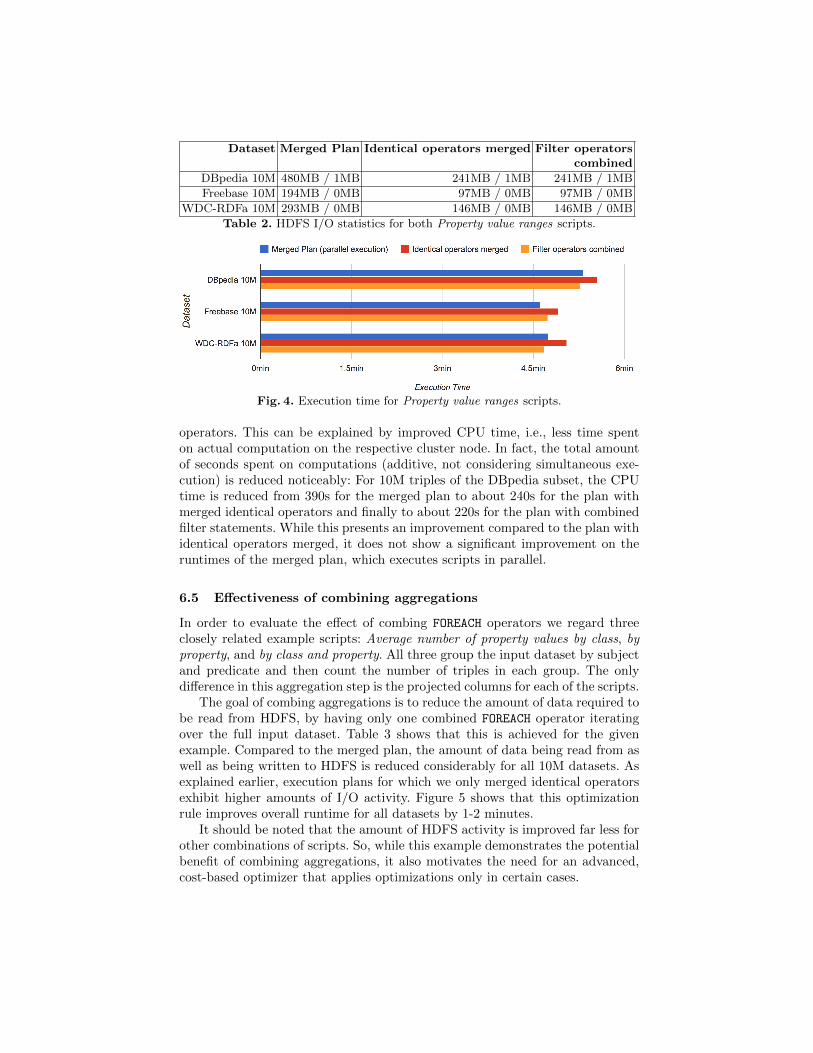
Dataset Merged Plan Identical operators merged Filter operatorscombined

DBpedia 10M 480MB / 1MB 241MB / 1MB 241MB / 1MB

Freebase 10M 194MB / 0MB 97MB / 0MB 97MB / 0MB

WDC-RDFa 10M 293MB / 0MB 146MB / 0MB 146MB / 0MB

Table 2. HDFS I/O statistics for both Property value ranges scripts.

Fig. 4. Execution time for Property value ranges scripts.

operators. This can be explained by improved CPU time, i.e., less time spenton actual computation on the respective cluster node. In fact, the total amountof seconds spent on computations (additive, not considering simultaneous exe-cution) is reduced noticeably: For 10M triples of the DBpedia subset, the CPUtime is reduced from 390s for the merged plan to about 240s for the plan withmerged identical operators and finally to about 220s for the plan with combinedfilter statements. While this presents an improvement compared to the plan withidentical operators merged, it does not show a significant improvement on theruntimes of the merged plan, which executes scripts in parallel.

6.5 Effectiveness of combining aggregations

In order to evaluate the effect of combing FOREACH operators we regard threeclosely related example scripts: Average number of property values by class, byproperty, and by class and property. All three group the input dataset by subjectand predicate and then count the number of triples in each group. The onlydifference in this aggregation step is the projected columns for each of the scripts.

The goal of combing aggregations is to reduce the amount of data required tobe read from HDFS, by having only one combined FOREACH operator iteratingover the full input dataset. Table 3 shows that this is achieved for the givenexample. Compared to the merged plan, the amount of data being read from aswell as being written to HDFS is reduced considerably for all 10M datasets. Asexplained earlier, execution plans for which we only merged identical operatorsexhibit higher amounts of I/O activity. Figure 5 shows that this optimizationrule improves overall runtime for all datasets by 1-2 minutes.

It should be noted that the amount of HDFS activity is improved far less forother combinations of scripts. So, while this example demonstrates the potentialbenefit of combining aggregations, it also motivates the need for an advanced,cost-based optimizer that applies optimizations only in certain cases.

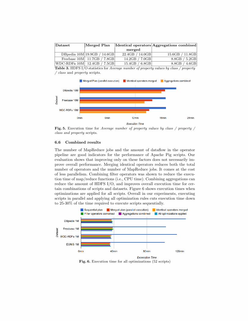
Dataset Merged Plan Identical operators Aggregations combinedmerged

DBpedia 10M 19.9GB / 14.6GB 22.4GB / 14.0GB 15.6GB / 11.8GB

Freebase 10M 11.7GB / 7.8GB 14.2GB / 7.0GB 8.8GB / 5.2GB

WDC-RDFa 10M 12.4GB / 7.5GB 15.4GB / 6.8GB 8.8GB / 4.6GB

Table 3. HDFS I/O statistics for Average number of property values by class / property/ class and property scripts.

Fig. 5. Execution time for Average number of property values by class / property /class and property scripts.

6.6 Combined results

The number of MapReduce jobs and the amount of dataflow in the operatorpipeline are good indicators for the performance of Apache Pig scripts. Ourevaluation shows that improving only on these factors does not necessarily im-prove overall performance. Merging identical operators reduces both the totalnumber of operators and the number of MapReduce jobs. It comes at the costof less parallelism. Combining filter operators was shown to reduce the execu-tion time of map/reduce functions (i.e., CPU time). Combining aggregations canreduce the amount of HDFS I/O, and improves overall execution time for cer-tain combinations of scripts and datasets. Figure 6 shows execution times whenoptimizations are applied for all scripts. Overall in our experiments, executingscripts in parallel and applying all optimization rules cuts execution time downto 25-30% of the time required to execute scripts sequentially.

Fig. 6. Execution time for all optimizations (52 scripts)

7 Conclusion

Existing work on data profiling can either not be applied to the area of LinkedData or exhibits considerable performance problems. To overcome this gap weintroduced a list of 56 data profiling tasks, implemented them as Apache Pigscripts, and analyzed the performance of executing them on an Apache Hadoopcluster. Thereby, we introduced three common techniques for improving perfor-mance, namely algorithmic optimization, parallelization and multi-script opti-mization. We experimentally demonstrated that they achieve their respectivegoals of optimizing the amount of MapReduce jobs or the amount of data ma-terialized between jobs.

In addition to the optimization techniques described in this paper, otheroptimization rules could be implemented. For instance, simple projections couldbe ignored in the logical optimization plans to allow further merging of operators,and aggregations based on similar groupings could be optimised to reduce theamount of redundant computation. Further, an advanced optimization strategyshould apply optimization rules only if the estimated overall performance gainis high enough and not as often as possible, as we do it now.

References

1. Naumann, F.: Data profiling revisited. SIGMOD Record 42(4) (2013)2. Gates, A., Dai, J., Nair, T.: Apache Pig’s Optimizer. IEEE Data Eng. Bull. 36(1)

(2013) 34–453. Khatchadourian, S., Consens, M.P.: ExpLOD: Summary-based exploration of in-

terlinking and RDF usage in the linked open data cloud. In: Proceedings of theExtended Semantic Web Conference (ESWC), Heraklion, Greece (2010) 272–287

4. Li, H.: Data Profiling for Semantic Web Data. In: Proceedings of the InternationalConference on Web Information Systems and Mining (WISM). (2012)

5. Langegger, A., Woß, W.: RDFStats – An extensible RDF statistics generator andlibrary. In: Proceedings of the International Workshop on Database and ExpertSystems Applications (DEXA), Los Alamitos, CA, USA (2009) 79–83

6. Auer, S., Demter, J., Martin, M., Lehmann, J.: LODStats – an extensible frame-work for high-performance dataset analytics. In: Proceedings for the InternationalConference on Knowledge Engineering and Knowledge Management (EKAW).(2012)

7. Bohm, C., Lorey, J., Naumann, F.: Creating VoiD descriptions for web-scale data.Journal of Web Semantics 9(3) (2011) 339–345

8. Bohm, C., Naumann, F., Abedjan, Z., Fenz, D., Grutze, T., Hefenbrock, D., Pohl,M., Sonnabend, D.: Profiling Linked Open Data with ProLOD. In: Proceedingsof the International Workshop on New Trends in Information Integration (NTII).(2010)

9. Abedjan, Z., Grutze, T., Jentzsch, A., Naumann, F.: Mining and profiling RDFdata with ProLOD++. In: Proceedings of the International Conference on DataEngineering (ICDE). (2014) Demo.

10. Sellis, T.K.: Multiple-query optimization. ACM Transactions on Database Systems(TODS) 13(1) (1988) 23–52