Logic, Optimization and Constraint Programming

J. N. Hooker •Graduate School of Industrial Administration

Carnegie Mellon University, Pittsburgh, PA 15213, USA

jh38@andrew.cmu.edu •April 2000; Revised November 2001

Because of their complementary strengths, optimization and constraint programming can

be profitably merged. Their integration has been the subject of increasing commercial and

research activity. This paper summarizes and contrasts the characteristics of the two fields;

in particular, how they use logical inference in different ways, and how these ways can

be combined. It sketches the intellectual background for recent efforts at integration. It

traces the history of logic-based methods in optimization and the development of constraint

programming in artificial intelligence. It concludes with a review of recent research, with

emphasis on schemes for integration, relaxation methods, and practical applications.

(Optimization, Constraint programming, Logic-based methods, Artificial Intelligence)

1. Introduction

Optimization and constraint programming are beginning to converge, despite their very

different origins. Optimization is primarily associated with mathematics and engineering,

while constraint programming developed much more recently in the computer science and

artificial intelligence communities. The two fields evolved more or less independently until

a very few years ago. Yet they have much in common and are applied to many of the

same problems. Both have enjoyed considerable commercial success. Most importantly for

present purposes, they have complementary strengths, and the last few years have seen

growing efforts to combine them.

Constraint programming, for example, offers a more flexible modeling framework than

mathematical programming. It not only permits more succinct models, but the models allow

one to exploit problem structure and direct the search. It relies on such logic-based methods

1

as domain reduction and constraint propagation to accelerate the search. Conversely, opti-

mization brings to the table a number of specialized techniques for highly structured problem

classes, such as linear programming problems or matching problems. It also provides a wide

range of relaxations, which are often indispensable for proving optimality. They may be

based on polyhedral analysis, in which case they take the form of cutting planes, or on the

solution of a dual problem, such as the Lagrangean dual.

The recent interaction between optimization and constraint programming

promises to change both fields. It is conceivable that portions of both will merge into a

single problem-solving technology for discrete and mixed discrete/continuous problems.

The aim of the present paper is to survey current activity in this area and sketch its intel-

lectual background. It begins with a general summary of the characteristics of optimization

and constraint programming: what they have in common, how they differ, and what each

can contribute to a combined approach. It then briefly recounts developments that led up to

the present state of the art. It traces the history of boolean and logic-based methods for opti-

mization, as well as the evolution of logic programming to constraint logic programming and

from there to the constraint programming “toolkits” of today. It concludes with a summary

of some current work. Since a proper tutorial in these ideas would require a much longer

paper, only a cursory explanation of key concepts is provided. A more complete treatment

is provided by Hooker (2000) as well as other sources cited in the context of particular topics

discussed below.

The emphasis in this paper is on exact methods, because this is where most of the

collaboration is now occurring. Yet optimization and constraint programming also share a

strong interest in heuristic methods. Interaction between the two fields in this area is hard

to characterize in general, but both are unaware of much recent research conducted by the

other. This may present a second opportunity for cross-fertilization in the near future.

2. Optimization and Constraint Programming

Compared

Optimization and constraint programming are similar enough to make their combination

possible, and yet different enough to make it profitable.

2

2.1 Two Areas of Commonality

There are at least two broad areas of commonality between optimization and constraint

programming. One is that both rely heavily on branching search, at least when an exact

method is required and the problem is combinatorial in nature.

The other is less obvious: both use logical inference methods to accelerate the search.

Constraint programming uses logical inference in the form of domain reduction and constraint

propagation. In optimization, logical inference takes forms that are not ordinarily recognized

as such, including cutting plane algorithms and certain duality theorems. A cutting plane,

for example, is a logical implication of a set of inequalities. Preprocessing algorithms for

mixed integer programming can also be viewed as limited forms of domain reduction and

constraint propagation.

When one takes a more historical view, the commonality becomes even more visible.

Boolean methods for operations research, which are based on logic processing, date from the

1950’s. Implicit enumeration methods for integer programming enjoyed only a brief moment

of fame in the 1970’s but can be seen as an early form of today’s constraint propagation

methods.

2.2 Two Main Differences

As the names might suggest, constraint programming seeks a feasible solution, and opti-

mization seeks an optimal solution. But this is a superficial distinction, as optimization is

easily incorporated into the algorithms of constraint programming by gradually tightening

a bound on the objective function value. The main differences between optimization and

constraint programming lie elsewhere.

2.2.1 Programming versus “Programming”

One key distinction between the two fields is that constraint programming formulates a

problem within a programming language. The formulation generally has a declarative look,

because one of the historical goals of the field is to allow one to integrate constraints into

programming. Yet the modeling language can give the modeler considerable control over

the search procedure. Thus the “programming” in constraint programming actually refers

to computer programming, unlike the “programming” in mathematical programming, which

recalls George Dantzig’s historical application of linear models to military logistics.

3

2.2.2 Constraint Propagation versus Relaxation

Another distinction is that constraint programming uses logical inference in different ways

than optimization uses it. It uses inference to reduce the search space directly through

such techniques as domain reduction and constraint propagation. Optimization uses infer-

ence (perhaps in the form of cutting planes) primarily to create better relaxations, which

accelerate the search indirectly.

Although optimization is not fundamentally distinguished by the fact that it optimizes,

the presence of cost and profit functions (whether they occur in an objective function or

constraints) has nonetheless taken the field in a different direction than constraint program-

ming. Cost and profit functions tend to contain many variables, representing the many

activities that can incur cost or contribute to profit. This often makes domain reduction and

constraint propagation ineffective.

The domain of a variable is the set of possible values it can take. Domain reduction uses

restrictions on the domain of one variable in a constraint to deduce that the other variables

can only take certain values, if the constraint is to be satisfied. If the constraint does not

contain too many variables, this can significantly reduce domains. The smaller domains are

passed to other constraints, where they are further reduced, thus implementing a form of

constraint propagation. If all goes well, a combination of branching search and constraint

propagation eventually reduce each variable’s domain to a single value, and a feasible solution

is identified.

When a constraint contains a cost or profit function of many variables, however, domain

reduction is ineffective. The optimization community escapes this impasse by using relax-

ation techniques, generally continuous relaxations. The community perhaps moved away

from the early implicit enumeration techniques, which resemble constraint propagation, be-

cause its business and engineering applications require measurement of cost and profit.

The constraint satisfaction community, by contrast, developed to a large degree through

consideration of problems whose constraints are binary; that is, they contain only two vari-

ables each. Many combinatorial problems discussed in the artificial intelligence literature are

of this sort. A standard example is the n-queens problem, which asks one to place n queens

on a chessboard so that no one attacks another. Restricting the domain of one variable in a

binary constraint can substantially reduce the domain of the other variable, and propagation

tends to be effective. It is not surprising that domain reduction and constraint propagation

4

methods have evolved from a field that historically emphasized binary constraints. These

methods can work well when there are no sums over cost or profit, and when the objective

is some such criterion as a min/max or minimum makespan.

It is sometimes said that constraint programming is more effective on “tightly con-

strained” problems, and optimization more effective on “loosely constrained” problems. This

is misleading, because one can typically make a problem more tightly constrained (even in-

feasible) by tightening the bound on a single constraint or the objective function. If the

constraint or objective function contains many variables, this is likely to make the problem

harder for constraint programming, not easier.

2.3 Opportunities for Integration

Many if not most practical problems have constraints that require relaxation as well as

constraints that propagate well. For this reason alone, it is natural to use a combination

of optimization and constraint satisfaction methods. In addition, the versatile modeling

framework of constraint satisfaction leads to models that are more readable and easier to

debug than traditional optimization models. Conversely, powerful optimization methods can

solve structured subproblems more efficiently than constraint programming methods.

2.3.1 Global Constraints

Still another inducement to integration is that constraint programming’s global constraints

provide a practical way for techniques from both fields to exploit problem structure. When

formulating a problem, one can often identify groups of constraints that exhibit a “global”

pattern. For instance, a set of constraints might require that jobs be scheduled so that they

do not overlap (or consume too many resources at any one time). These constraints can be

represented by a single global constraint, in this case a cumulative constraint.

An equally popular global constraint is all-different, which requires that a set of variables

all take different values. It can be used to formulate the traveling salesman problem, for

example, with a single constraint, rather than exponentially many as in the most popular

integer programming model. Let xj denote the jth city visited by the salesman, and let cij

be the distance from city i to city j. Then the traveling salesman problem can be written

minimizen∑

j=1

cxjxj+1

subject to all-different(x1, . . . , xn)

(1)

5

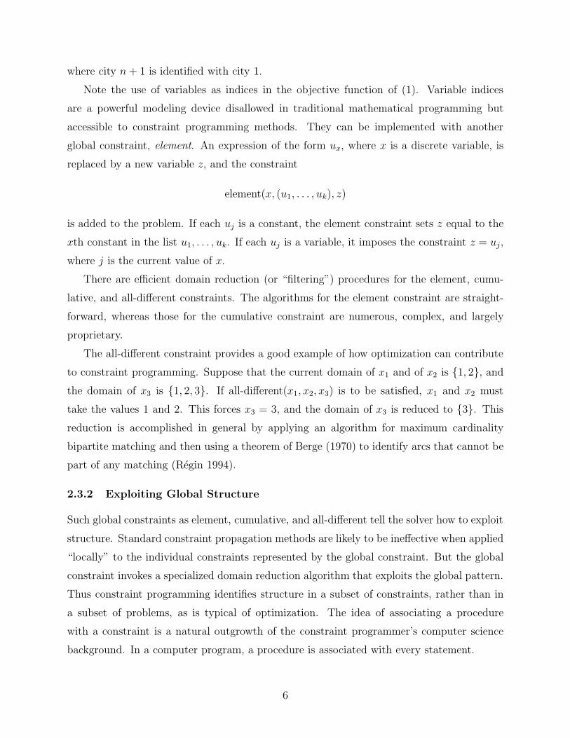
where city n + 1 is identified with city 1.

Note the use of variables as indices in the objective function of (1). Variable indices

are a powerful modeling device disallowed in traditional mathematical programming but

accessible to constraint programming methods. They can be implemented with another

global constraint, element. An expression of the form ux, where x is a discrete variable, is

replaced by a new variable z, and the constraint

element(x, (u1, . . . , uk), z)

is added to the problem. If each uj is a constant, the element constraint sets z equal to the

xth constant in the list u1, . . . , uk. If each uj is a variable, it imposes the constraint z = uj,

where j is the current value of x.

There are efficient domain reduction (or “filtering”) procedures for the element, cumu-

lative, and all-different constraints. The algorithms for the element constraint are straight-

forward, whereas those for the cumulative constraint are numerous, complex, and largely

proprietary.

The all-different constraint provides a good example of how optimization can contribute

to constraint programming. Suppose that the current domain of x1 and of x2 is {1, 2}, and

the domain of x3 is {1, 2, 3}. If all-different(x1, x2, x3) is to be satisfied, x1 and x2 must

take the values 1 and 2. This forces x3 = 3, and the domain of x3 is reduced to {3}. This

reduction is accomplished in general by applying an algorithm for maximum cardinality

bipartite matching and then using a theorem of Berge (1970) to identify arcs that cannot be

part of any matching (Regin 1994).

2.3.2 Exploiting Global Structure

Such global constraints as element, cumulative, and all-different tell the solver how to exploit

structure. Standard constraint propagation methods are likely to be ineffective when applied

“locally” to the individual constraints represented by the global constraint. But the global

constraint invokes a specialized domain reduction algorithm that exploits the global pattern.

Thus constraint programming identifies structure in a subset of constraints, rather than in

a subset of problems, as is typical of optimization. The idea of associating a procedure

with a constraint is a natural outgrowth of the constraint programmer’s computer science

background. In a computer program, a procedure is associated with every statement.

6

Global constraints also take advantage of the practitioner’s expertise. The popular global

constraints evolved because they formulate situations that commonly occur in practice. An

expert in the problem domain can recognize these patterns in practical problems, perhaps

more readily than the developers of a constraint programming system. By using the ap-

propriate global constraints, a practitioner who knows little about solution technology au-

tomatically invokes the best available domain reduction algorithms that are relevant to the

problem.

Global constraints can provide this same service to optimization methods. For example,

a global constraint that represents inequality constraints with special structure can bring

along any known cutting planes for them. Much cutting plane technology now goes un-

used in commercial solvers because there is no suitable framework for identifying when it

applies. Existing optimization solvers identify some types of structure, such as network flow

constraints. But they do so only in a limited way, and in any event it is inefficient to oblit-

erate structure by modeling with an atomistic vocabulary of inequalities and equations and

then try to rediscover the structure automatically. The vast literature on relaxations can be

put to work if practitioners write their models with as many global constraints as possible.

This means that modelers must change their modeling habits, but they may welcome such

a change.

In the current state of the art, a global constraint may have no known relaxation. In this

case the challenge to optimization is clear: use the well-developed theory on this subject to

find one.

3. Logic-Based Methods in Optimization

Boolean and logic-based methods have a long history in discrete optimization. Their develop-

ment might be organized into two overlapping stages. One is the classical boolean tradition,

which traces back to the late 1950’s and continues to receive attention, even though it has

never achieved mainstream status to the same extent as integer programming. The second

stage introduced logical ideas into integer and mixed integer programming. This research

began with the implicit enumeration and disjunctive programming ideas of the 1970’s and

likewise continues to the present day. A more detailed treatment of this history is provided

by Hooker (2000).

7

3.1 Boolean Methods

George Boole’s small book, The Mathematical Analysis of Logic (1847), laid the foundation

for all subsequent work in computational logic. In the 1950s and 1960s, the new field of

operations research was quick to notice the parallel between his two-valued logic and 0-1

programming (Fortet 1959,1960; Hansen et al. 1993). The initial phase of research in boolean

methods culminated in the treatise of Hammer and Rudeanu (1968). Related papers from

this era include those of Hammer, Rosenberg, and Rudeanu (1963); Balas and Jeroslow

(1972); Granot and Hammer (1971,1975); and Hammer and Peled (1972).

These and subsequent investigators introduced three ideas that today play a role in the

integration of optimization with constraint programming: (a) nonserial dynamic program-

ming and the concept of induced width, (b) continuous relaxations for logical constraints,

and (c) derivation of logical propositions from constraints.

3.1.1 Nonserial Dynamic Programming

Nonserial dynamic programming is implicit in Hammer and Rudeanu’s “basic method” for

pseudoboolean optimization (i.e., optimization of a real-valued function of boolean variables).

Bertele and Brioschi (1972) independently developed the concept in the late 1960s and early

1970s, but boolean research took it an important step further. When Crama, Hansen, and

Jaumard (1990) revisited the basic method more than twenty years after its invention, they

discovered that it can exploit the structure of what they called the problem’s co-occurrence

graph. The same graph occurs in the constraint programming literature, where it is called

the dependency graph (or primal graph). Crama et al. found that the complexity of the

algorithm depends on a property of the graph known in the artificial intelligence community

as its induced width, which is defined for a given ordering of the variables. Consideration of

the variables in the right order may result in a small induced width and faster solution.

To elaborate on this a bit, the dependency graph G for an optimization problem contains

a vertex for each variable xj and an edge (i, j) whenever xi and xj occur in the same

constraint, or the same term of the objective function. To define the width of G, suppose

that one removes vertices from G in the order n, n− 1, . . . , 1. If dj is the degree of j at the

time of its removal, the width of G with respect to the ordering 1, . . . , n is the maximum of dj

over all j. Now suppose that just before vertex j is removed, one adds edges to G as needed

to link all vertices that are connected to j by an edge. The induced width of G with respect

8

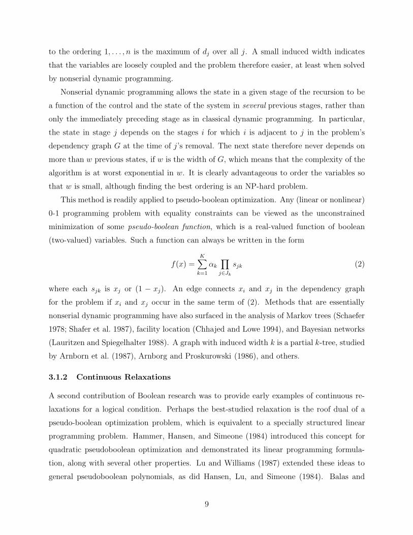
to the ordering 1, . . . , n is the maximum of dj over all j. A small induced width indicates

that the variables are loosely coupled and the problem therefore easier, at least when solved

by nonserial dynamic programming.

Nonserial dynamic programming allows the state in a given stage of the recursion to be

a function of the control and the state of the system in several previous stages, rather than

only the immediately preceding stage as in classical dynamic programming. In particular,

the state in stage j depends on the stages i for which i is adjacent to j in the problem’s

dependency graph G at the time of j’s removal. The next state therefore never depends on

more than w previous states, if w is the width of G, which means that the complexity of the

algorithm is at worst exponential in w. It is clearly advantageous to order the variables so

that w is small, although finding the best ordering is an NP-hard problem.

This method is readily applied to pseudo-boolean optimization. Any (linear or nonlinear)

0-1 programming problem with equality constraints can be viewed as the unconstrained

minimization of some pseudo-boolean function, which is a real-valued function of boolean

(two-valued) variables. Such a function can always be written in the form

f(x) =K∑

k=1

αk

∏j∈Jk

sjk (2)

where each sjk is xj or (1 − xj). An edge connects xi and xj in the dependency graph

for the problem if xi and xj occur in the same term of (2). Methods that are essentially

nonserial dynamic programming have also surfaced in the analysis of Markov trees (Schaefer

1978; Shafer et al. 1987), facility location (Chhajed and Lowe 1994), and Bayesian networks

(Lauritzen and Spiegelhalter 1988). A graph with induced width k is a partial k-tree, studied

by Arnborn et al. (1987), Arnborg and Proskurowski (1986), and others.

3.1.2 Continuous Relaxations

A second contribution of Boolean research was to provide early examples of continuous re-

laxations for a logical condition. Perhaps the best-studied relaxation is the roof dual of a

pseudo-boolean optimization problem, which is equivalent to a specially structured linear

programming problem. Hammer, Hansen, and Simeone (1984) introduced this concept for

quadratic pseudoboolean optimization and demonstrated its linear programming formula-

tion, along with several other properties. Lu and Williams (1987) extended these ideas to

general pseudoboolean polynomials, as did Hansen, Lu, and Simeone (1984). Balas and

9

Mazzola (1980a,1980b) studied a family of bounding functions of which the roof bound is

one sort. The roof dual turns out to be an instance of the well-known Lagrangean dual, ap-

plied to a particular integer programming formulation of the problem. Adams and Dearing

(1994) demonstrated this for the quadratic case, and Adams, Billionnet, and Sutter (1990)

generalized the result. Today the formulation of continuous relaxations for logical and other

discrete constraints is an important research program for the integration of optimization and

constraint programming.

3.1.3 Implied Constraints

A third development in boolean research was the derivation of logical implications from 0-1

inequality constraints. The derived implications can be used in either of two ways. They

have been primarily used as cutting planes that strengthen the continuous relaxation of the

inequalities, as for example in Balas and Mazzola (1980a,1980b). Of greater interest here,

however, is the purely logical use of derived implications. One can solve a 0-1 problem by

reducing its constraints to logical form so that inference algorithms can be applied. The

most advanced effort in this direction is Barth’s pseudo-boolean solver (1995).

The early boolean literature shows how to derive logical clauses from linear or nonlinear

0-1 inequalities. A clause is a disjunction of literals, each of which is a logical variable xj

or its negation ¬xj . For instance, the clause x1 ∨ x2 ∨ ¬x3 states that x1 is true or x2 is

true or x3 is false (where the “or” is inclusive). A simple recursive algorithm of Granot and

Hammer (1971) obtains all nonredundant clauses implied by a single linear 0-1 inequality.

Granot and Hammer (1975) also stated an algorithm for deriving all clausal implications of

a single nonlinear inequality.

Barth took this a step further by deriving cardinality clauses from 0-1 inequalities. A

cardinality clause says that at least k of a set of literals are true (k = 1 in an ordinary

clause). Cardinality clauses tend to capture numerical ideas more succinctly than ordinary

clauses and yet retain many of their algorithmic advantages. Barth’s derivation is based on

a complete inference method for 0-1 inequalities (Hooker 1992) and takes full advantage of

the problem structure to obtain nonredundant clauses efficiently.

Another motivation for deriving constraints is to make a problem more nearly “consis-

tent” (discussed below), so as to reduce backtracking. Constraints derived for this reason

can be contrasted with cutting planes, which are derived with the different motivation of

strengthening a continuous relaxation of the problem. To appreciate the difference, note

10

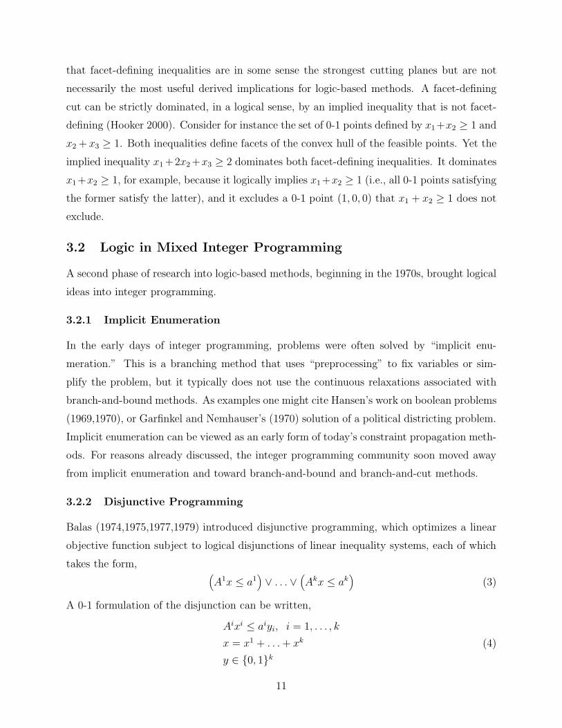
that facet-defining inequalities are in some sense the strongest cutting planes but are not

necessarily the most useful derived implications for logic-based methods. A facet-defining

cut can be strictly dominated, in a logical sense, by an implied inequality that is not facet-

defining (Hooker 2000). Consider for instance the set of 0-1 points defined by x1+x2 ≥ 1 and

x2 + x3 ≥ 1. Both inequalities define facets of the convex hull of the feasible points. Yet the

implied inequality x1 +2x2 +x3 ≥ 2 dominates both facet-defining inequalities. It dominates

x1+x2 ≥ 1, for example, because it logically implies x1 +x2 ≥ 1 (i.e., all 0-1 points satisfying

the former satisfy the latter), and it excludes a 0-1 point (1, 0, 0) that x1 + x2 ≥ 1 does not

exclude.

3.2 Logic in Mixed Integer Programming

A second phase of research into logic-based methods, beginning in the 1970s, brought logical

ideas into integer programming.

3.2.1 Implicit Enumeration

In the early days of integer programming, problems were often solved by “implicit enu-

meration.” This is a branching method that uses “preprocessing” to fix variables or sim-

plify the problem, but it typically does not use the continuous relaxations associated with

branch-and-bound methods. As examples one might cite Hansen’s work on boolean problems

(1969,1970), or Garfinkel and Nemhauser’s (1970) solution of a political districting problem.

Implicit enumeration can be viewed as an early form of today’s constraint propagation meth-

ods. For reasons already discussed, the integer programming community soon moved away

from implicit enumeration and toward branch-and-bound and branch-and-cut methods.

3.2.2 Disjunctive Programming

Balas (1974,1975,1977,1979) introduced disjunctive programming, which optimizes a linear

objective function subject to logical disjunctions of linear inequality systems, each of which

takes the form, (A1x ≤ a1

)∨ . . . ∨

(Akx ≤ ak

)(3)

A 0-1 formulation of the disjunction can be written,

Aixi ≤ aiyi, i = 1, . . . , k

x = x1 + . . . + xk

y ∈ {0, 1}k(4)

11

The continuous relaxation of this formulation (obtained by replacing each yi ∈ {0, 1} by

0 ≤ yi ≤ 1) provides a convex hull relaxation of the feasible set of (3). It does so at the cost

of adding variables yi and vectors xi of variables. Nonetheless (4) provides a tool for ob-

taining continuous relaxations of logical constraints, including constraints other than simple

disjunctions. Sometimes the additional variables can be projected out, or the formulation

otherwise simplified.

In the meantime Jeroslow brought his background in formal logic to integer programming

(e.g., Balas and Jeroslow 1972). He proved what is perhaps the only general theorem of

mixed integer modeling: that representability by a mixed integer model is the same as

representability by disjunctive models of the form (4). From this he derived that a subset of

continuous space is the feasible set of some mixed integer model if and only if it is the union

of finitely many polyhedra, all of which have the same set of recession directions. He proved a

similar result for mixed integer nonlinear programming (1987,1989). His analysis provides a

general tool for obtaining continuous relaxations for nonconvex regions of continuous space,

which again may or may not be practical in a given case.

3.3 Links between Logic and Mathematical Programming

Williams (1976,1977,1987,1991,1995) was among the first to point out parallels between

logic and mathematical programming (see also Williams and Yan 2001). Laundy (1986),

Beaumont (1990), and Wilson (1990,1995,1996) also contributed to this area.

3.3.1 Connections with Resolution

To take one parallel, the well-known resolution method for logical inference can be viewed as

Fourier-Motzkin elimination plus rounding. Fourier-Motzkin elimination was one of the ear-

liest linear programming algorithms, proposed for instance by Boole (Hailperin 1976,1986).

Given two logical clauses for which exactly one variable xj occurs positively in one and neg-

atively in the other, the resolvent of the clauses is the clause consisting of all the literals in

either clause except xj and ¬xj . For example, the resolvent of the clauses

x1 ∨ x2 ∨ ¬x3

¬x1 ∨ x2 ∨ x4(5)

is x2 ∨ ¬x3 ∨ x4. The logician Quine (1952,1955) showed that repeated application of this

resolution step to a clause set, and to the resolvents generated from the clause set, derives all

12

clauses that are implied by the set. To see the connection with Fourier-Motzkin elimination,

write the clauses (5) as 0-1 inequalities:

x1 + x2 + (1− x3) ≥ 1

(1− x1) + x2 + x4 ≥ 1

where 0-1 values of xj correspond to false and true, respectively. If one eliminates x1,

the result is the 0-1 inequality x2 + 12(1 − x3) + 1

2x4 ≥ 1

2, which dominates x2 + (1 −

x3) + x4 ≥ 12. The right-hand side can now be rounded up to obtain the resolvent of

(5). As this example might suggest, a resolvent is a rank 1 Chvatal cutting plane. Further

connections between resolution and cutting planes are described by Hooker (1988,1989,1992).

For example, deriving from a clause set all clauses that are rank 1 cuts is equivalent to

applying the unit resolution algorithm or the input resolution algorithm to the clause set

(Hooker 1989). (In unit resolution, at least one of the two parents of a resolvent contains a

single literal. In input resolution, at least one parent is a member of the original clause set.)

Resolution is also related to linear programming duality, as shown by Jeroslow and Wang

(1989) in the case of Horn clauses, and generalized to gain-free Leontief flows, as shown by

Jeroslow et al. (1989). Horn clauses are those with at most one positive literal and are

convenient because unit resolution can check their satisfiability in linear time. Jeroslow and

Wang pointed out that linear programming can also check their satisfiability. Chandru and

Hooker (1991) showed that the underlying reason for this is related to an integer program-

ming rounding theorem of Chandrasekaran (1984). They used this fact to generalize Horn

clauses to a much larger class of “extended Horn” clauses that have the same convenient

properties, a class that was further extended by Schlipf et al. (1995).

Connections such as these suggest that optimization can help solve logical inference

problems, as well as the reverse. In fact there is a stream of research that does just this,

summarized in a book of Chandru and Hooker (1999). Recent work in this area began with

Blair, Jeroslow and Lowe’s (1988) use of branch-and-bound search to solve the satisfiabil-

ity problem. The link between resolution and cutting planes described above leads to a

specialized branch-and-cut method for the same problem (Hooker and Fedjki 1990). Recent

work shows that integer programming and Lagrangean relaxation can yield a state-of-the-art

method for the satisfiability and incremental satisfiability problems (Bennaceur et al. 1998).

The earliest application of optimization to logic, however, seems to be Boole’s application

of linear programming to probabilistic logic (Boole 1952; Hailperin 1976). (It was in this

connection that he used elimination to solve linear programming problems.) Optimization

13

can also solve inference problems in first order predicate logic, modal logic, such belief logics

as Dempster-Shafer theory, and nonmonotonic logic.

3.3.2 Mixed Logical/Linear Programming

Mixed logical/linear programming (MLLP) might be defined roughly as mixed discrete/linear

programming in which the discrete aspects of the problem are written directly as logical

conditions rather than with integer variables. For example, disjunctions of linear systems

are written as (2) rather than with the convex hull formulation (3) or the big-M formulation

Aix ≤ ai + Mi(1− yi), i = 1, . . . , k

y ∈ {0, 1}k (6)

A logical formulation can be more natural and require fewer variables, but it raises the

question as to how a relaxation can be formulated. The traditional integer programming

formulation comes with a ready-made relaxation, obtained by dropping the integrality re-

quirement for variables. Solution of the relaxation provides a bound on the optimal value

that can be essential for proving optimality.

Beaumont (1990) was apparently the first to address this issue in an MLLP context.

He obtained a relaxation for disjunctions (2) in which the linear systems Aix ≤ bi are

single inequalities aix ≤ bi. He did so by projecting the continuous relaxation of the big-

M formulation (6) onto the continuous variables x. This projection simplifies to a single

“elementary” inequality (k∑

i=1

ai

Mi

)x ≤

k∑i=1

bi

Mi

+ k − 1 (7)

An inexpensive way to tighten the inequality is presented by Hooker and Osorio (1999).

Beaumont also identified some valid inequalities that are facet-defining under certain (strong)

conditions.

A generalization of Beaumont’s approach is to introduce propositional variables and to

associate at least some of them with linear systems. Logical constraints can then express

complex logical relationships between linear systems. One can also process the logical con-

straints to fix values, etc., as proposed by Hooker (1994) and Grossmann et al. (1994). In the

latter, Grossmann et al. designed chemical processing networks by associating a propositional

variable xj with processing units. When xj is true, processing unit j and its associated arcs

are present in the network. When xj is false, flow through unit j is forced to zero. Purely

logical constraints are written to ensure that a unit is not installed unless units that supply

14

its feedstock and receive its output are also present. A number of processing network de-

sign, process scheduling, and truss structure design problems have been solved with the help

of logic (Bollapragada et al. 2001; Cagan et al. 1997; Pinto and Grossmann 1997; Raman

and Grossmann 1991,1993,1994; Turkay and Grossmann 1996). Some of these problems

are nonlinear and are attacked with mixed logical/nonlinear programming (MLNLP). A key

advantage of MLNLP is that situations in which an activity level drops to zero can be dis-

tinguished as logically distinct states with different associated equations, thus avoiding the

singularities that tend to occur in traditional models.

A general approach to MLLP was developed in the mid-1990’s (Osorio and Hooker 1996;

Hooker and Osorio 1999). In particular, these authors critiqued the role of integer variables

in optimization and suggested guidelines for when a logical formulation is better. They,

along with Little and Darby-Dowman (1995), proposed incorporating constraint program-

ming methods into mathematical programming.

4. Constraint Programming and Constraint

Satisfaction

Constraint programming can be conceived generally as the embedding of constraints within

a programming language. This combination of declarative and procedural modeling gives

the user some control over how the problem is solved, even while retaining the ability to

state constraints declaratively.

It is far from obvious how declarative and procedural formulations may be combined. In

a procedural code, for example, it is common to assign a variable different values at various

points in the code. This is nonsense in a declarative formulation, since it is contradictory to

state constraints that assign the same variable different values. The developments that gave

rise to constraint programming can in large part be seen as attempts to address this problem.

They began with logic programming and led to a number of alternative approaches, such as

constraint handling rules, concurrent constraint programming, constraint logic programming,

and constraint programming. Constraint programming “toolkits” represent a somewhat

more procedural version of constraint logic programming and are perhaps the most widely

used alternative.

Two main bodies of theory underlie these developments. One is the theory of first-order

logic on which logic programming is based, which was later generalized to encompass con-

15

straint logic programming. The other is a theory of search developed in the constraint satis-

faction literature, which deals with such topics as consistency, search orders, the dependency

graph, and various measures of its width.

Lloyd’s text (1984) provides a good introduction to logic programming, which is further

exposited in Clocksin and Mellish (1984) and Sterling and Shapiro (1986). Tsang (1993)

provides excellent coverage of the theory of constraint satisfaction. Van Hentenryck (1989)

wrote an early exposition of constraint logic programming, while Marriott and Stuckey’s text

(1998) is a valuable resource for recent work in constraint programming and constraint logic

programming. Chapters 10-11 of Hooker (2000) summarize these ideas.

4.1 Programming with Constraints

Several schemes have been proposed for embedding constraints in a programming language:

constraint logic programming, constraint programming “toolkits,” concurrent constraint pro-

gramming, and time-index variables. All of these owe a conceptual debt to logic program-

ming.

4.1.1 Logic Programming

One of the central themes of logic programming is to combine the declarative and the proce-

dural. As originally conceived by Kowalski (1979) and Colmerauer (1982), a logic program

can be read two ways: as a series of logical propositions that state conditions a solution must

satisfy, and as instructions for how to search for a solution.

To take a very simple example, rules 1 and 2 in the following logic program can be read

as a recursive definition of an ancestor:

1. ancestor(X, Y )←parent(X, Y ).

2. ancestor(X, Z)←parent(X, Y ),ancestor(Y, Z).

3. parent(a, b).4. parent(b, c).

(8)

Here X, Y and Z are variables, and a, b and c are constants. Rule 1 says that X is an

ancestor of Y if X is a parent of Y . One can deduce from statements 1 through 4 that a is

c’s ancestor. This is the declarative reading of the program.

16

ancestor(a, c)������

Rule 1

parent(a, c)"""""

Rule 3

fail

bbbbbRule 4

fail

HHHHHHRule 2

parent(a, Y )ancestor(Y, c)

Rule 3

ancestor(b, c)

Rule 1

parent(b, c)

Rule 4

succeed

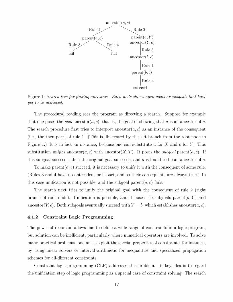
Figure 1: Search tree for finding ancestors. Each node shows open goals or subgoals that haveyet to be achieved.

The procedural reading sees the program as directing a search. Suppose for example

that one poses the goal ancestor(a, c); that is, the goal of showing that a is an ancestor of c.

The search procedure first tries to interpret ancestor(a, c) as an instance of the consequent

(i.e., the then-part) of rule 1. (This is illustrated by the left branch from the root node in

Figure 1.) It is in fact an instance, because one can substitute a for X and c for Y . This

substitution unifies ancestor(a, c) with ancestor(X, Y ). It poses the subgoal parent(a, c). If

this subgoal succeeds, then the original goal succeeds, and a is found to be an ancestor of c.

To make parent(a, c) succeed, it is necessary to unify it with the consequent of some rule.

(Rules 3 and 4 have no antecedent or if-part, and so their consequents are always true.) In

this case unification is not possible, and the subgoal parent(a, c) fails.

The search next tries to unify the original goal with the consequent of rule 2 (right

branch of root node). Unification is possible, and it poses the subgoals parent(a, Y ) and

ancestor(Y, c). Both subgoals eventually succeed with Y = b, which establishes ancestor(a, c).

4.1.2 Constraint Logic Programming

The power of recursion allows one to define a wide range of constraints in a logic program,

but solution can be inefficient, particularly where numerical operators are involved. To solve

many practical problems, one must exploit the special properties of constraints, for instance,

by using linear solvers or interval arithmetic for inequalities and specialized propagation

schemes for all-different constraints.

Constraint logic programming (CLP) addresses this problem. Its key idea is to regard

the unification step of logic programming as a special case of constraint solving. The search

17

ancestor(a, c)������

Rule 1

parent(X,Y )(X,Y ) = (a, b)

"""""Rule 3

(X,Y ) = (a, c)(X,Y ) = (a, b)

fail

bbbbbRule 4

(X,Y ) = (a, c)(X,Y ) = (b, c)

fail

HHHHHHRule 2

parent(X,Y )ancestor(Y,Z)(X,Z) = (a, c)

Rule 3ancestor(Y,Z)

(X,Y,Z) = (a, b, c)

Rule 1

parent(X ′, Y ′)(X,Y,Z) = (a, b, c)(X ′, Y ′) = (Y,Z)

Rule 4

(X,Y,Z) = (a, b, c)(X ′, Y ′) = (Y,Z)(X ′, Y ′) = (b, c)

succeed

Figure 2: Search tree in which unification is interpreted as constraint solving.

tree of Figure 1 becomes the search tree of Figure 2. For instance, unifying ancestor(a, c)

with ancestor(X, Z) is tantamount to solving the equation (a, c) = (X, Z) for X and Z. This

is illustrated in the right descendant of the root node in the figure. The process continues

as before, except that constraints are accumulated into a constraint store as subgoals are

discharged. At the leaf nodes only constraints remain, and the node succeeds if they are

soluble.

In a pure logic programming language such as the early PROLOG (Colmerauer’s ab-

breviation for programmation en logique), the constraint store contains only equations that

unify predicates. One obtains CLP by expanding the repertory of constraints and variables.

Marriott and Stuckey (1998) identify the first CLP system to be Colmerauer’s 1982 lan-

guage PROLOG II (Colmerauer 1982), in which unification requires solution of disequations

as well as equations. Jaffar and Stuckey (1986) showed in 1986 that the theory of pure

logic programming can be extended to PROLOG II. Jaffar and Lassez (1987) pointed out

that PROLOG II is a special case of a general scheme in which unification is viewed as a

constraint-solving problem. The term “constraint logic programming” originates from this

paper.

Several CLP systems quickly followed. Colmerauer and his colleagues added constraint

solving over strings, boolean variables, and real linear arithmetic in PROLOG III (Colmer-

18

auer 1987,1990). Jaffar and Michaylov (1987) and Jaffar et al. (1992) added real arithmetic

to obtain CLP(<). Dincbas et al. (1988) and Aggoun et al. (1988) added constraints over

finite domains, including domains of integers, in their system CHIP.

Although unification is not a hard problem in classical PROLOG, it can quickly become

hard when one adds such constraints as inequalities over integers or constraints over finite

domains. For this reason the constraint solver may be incomplete; it may fail to find a solution

even if one exists. More often constraint solvers narrow the range of possible solutions

through domain reduction. In such cases the constraint store does not contain the hard

constraints but only such very simple ones as “in-domain” constraints; i.e., constraints stating

that each variable must take a value within a certain domain. Domain reduction algorithms

add to the constraint store by deriving new in-domain constraints.

If the constraint solvers and domain reduction fail to find a solution (i.e., fail to reduce the

domains to singletons), one can branch further by splitting variable domains. The constraint

solvers are reapplied after branching, and the domains further reduced. This in turn reduces

the amount of further branching that is necessary.

Constraint programming “toolkits” are based on CLP but do not require the model to

be written in a strict logic programming framework. Early toolkits include the CHARME

system of Oplobedu, Marcovich, and Tourbier (1989) and the PECOS language of Puget

(1992), both of which evolved from CHIP. Puget (1994,1995) later developed the initial

ILOG Solver, which embeds constraints in the object-oriented language C++. The toolkit

provides a library of C++ objects that implement many of the same constraint propagation

algorithms found in CLP systems. Constraints are defined by using the abstraction and

overloading facilities of C++.

4.1.3 Links with Optimization

Linear and even nonlinear programming have played a role in constraint programming sys-

tems for some years. They appear in such systems as CHIP (Aggoun et al. 1987), the ILOG

Solver (Puget 1994) and PROLOG III and IV (Colmerauer 1990,1996). Beringer and De

Backer (1995) used linear programming to tighten upper and lower bounds on continuous

variables. Solnon (1997) proposed that a linear programming solver minimize and maximize

each variable, to obtain bounds on it, at each node of a branch-and-bound tree. Using a

somewhat different approach, McAloon and Tretkoff (1996) developed a system 2LP that

allows one to invoke linear programming in a script that implements logic-based modeling.

19

4.2 Theories of Search

The constraints community has developed at least two related theories of search. One, which

comprises much of the constraint satisfaction field, examines factors that govern the amount

of backtracking necessary to complete a branching search. It is fully explained in Tsang’s text

(1993) and summarized from a mathematical programming perspective by Hooker (1997).

Another explores the idea of constraint-based search, which combines inference and branch-

ing. It is exposited in Chapter 18 of Hooker (2000).

4.2.1 Constraint Satisfaction

The fundamental concept of constraint satisfaction is that of a consistent constraint set,

which is not the same as a satisfiable or feasible constraint set. A consistent constraint set

is fully ramified in the sense that all of its implications are explicitly stated by constraints.

To be more precise, let the vector x = (x1, . . . , xn) be arbitrarily partitioned x = (x1, x2).

Then the assignment x1 = v1 is a partial assignment (or compound label). By convention, a

partial assignment x1 = v1 can violate a constraint only when x1 contains all the variables

that occur in the constraint. Let D1 be the cartesian product of the domains of the variables

in x1, and similarly for D2. Then if v1 ∈ D1, the partial assignment x1 = v1 is redundant

for a constraint set C if it violates no constraints in C but cannot be extended to a feasible

solution. That is, x1 = v1 violates no constraint in C, but (x1, x2) = (v1, v2) is infeasible

for all v2 ∈ D2. A constraint set is consistent if there are no redundant partial assignments.

In other words, any redundant partial assignment is explicitly ruled out because it violates

some constraint. It is not hard to see that one can find a feasible solution for a consistent

constraint set, if one exists, without backtracking.

The concept of consistency also provides a theoretical link between the amount of back-

tracking and the branching order, a link that has not been achieved in the optimization

literature. A constraint set C is k-consistent if for any partition x = (x1, x2) in which x1

contains k − 1 variables, and for any xj in x2, any partial assignment x1 = v1 that violates

no constraints in C can be extended to an assignment (x1, xj) = (v1, vj) that violates no

constraints in C, where vj ∈ Dj . A constraint set is strongly k-consistent if it is t-consistent

for t = 1, . . . , k. Suppose that one seeks a solution for a strongly k-consistent constraint

set C by branching on the variables in the order x1, . . . , xk. Freuder (1982) showed that no

backtracking will occur if the dependency graph for C has width less than k with respect to

20

the ordering x1 . . . , xn.

Consistency is closely related to logical inference. For instance, applying the resolution

algorithm to a set of logical clauses makes the set consistent. If the algorithm is modified so

that it generates only resolvents with fewer than k literals, it makes the clause set strongly k-

consistent. In general, drawing inferences from a constraint set tends to make it more nearly

consistent and to reduce backtracking. This contrasts with mathematical programming,

where inferences in the form of cutting planes are drawn to tighten the continuous relaxation

of the problem. Cutting planes can have the ancillary effect of making the constraint set

more nearly consistent, although the optimization literature has never formally recognized

the concept of consistency.

There are other results that connect backtracking with the search order. Dechter and

Pearl (1988) showed that a given search order results in no backtracking if the constraint

set has adaptive consistency (a kind of local consistency) with respect to that ordering. The

bandwidth of a constraint set’s dependency graph with respect to an ordering xi1 , . . . , xin is

the maximum of |j − k| over all arcs (ij , ik) in the dependency graph. The bandwidth with

respect to an ordering is the maximum number of levels one must backtrack on encountering

an infeasible solution during a tree search that branches on variables in that same order.

The bandwidth is an upper bound on the induced width (Zabih 1990), and a minimum

bandwidth ordering can be computed by dynamic programming (Gurari and Sudborough

1984; Saxe 1980).

Because commercial solvers process constraints primarily by reducing variable domains,

they tend to focus on types of consistency that relate to individual domains. The ideal

is hyperarc consistency, which is achieved when the domains have been reduced as much as

possible. Thus a constraint set is hyperarc consistent when any individual assignment xj = v

that violates no constraint is part of some feasible solution. Hyperarc consistency does not

imply consistency; it implies 2-consistency but is not equivalent to it. When all the con-

straints are binary (contain two variables), hyperarc consistency reduces to arc consistency,

which in this case is equivalent to 2-consistency. Domain reduction procedures often do not

achieve hyperarc consistency. A popular weaker form of consistency is bounds consistency,

which applies to integer-valued variables. A constraint set is bounds consistent when any

integer-valued variable assumes the smallest value in its domain in some feasible solution

and assumes the largest value in its domain in some feasible solution. Bounds consistency

can be achieved by interval arithmetic, which is a standard feature of constraint program-

21

ming systems but is especially important in such nonlinear equation solvers as Newton (Van

Hentenryck and Michel 1997; Van Hentenryck et al. 1998).

Domain reduction can be viewed as the generation of “in-domain” constraints that restrict

the values of variables to smaller domains. The resulting set of in-domain constraints is in

effect a relaxation of the problem. Constraints generated by some other type of consistency

maintenance can conceivably issue a stronger relaxation that consists of more interesting

constraints.

4.2.2 Constraint-Based Search

Depth-first branching and constraint-based search represent opposite poles of a family of

search methods. Depth-first branching incurs little overhead but is very inflexible. Once it

begins to explore a subtree, it must search the entire subtree even when there seems little

chance of finding a solution in it. Constraint-based search can be much more intelligent, but

the mechanism that guides the search exacts a computational toll. After exploring an initial

trial solution, it generates a constraint, called a nogood, that rules out the trial solution

just explored (and perhaps others that must fail for the same reason). At any point in the

search, a set of nogoods have been generated by past trial solutions. The next candidate

solution is identified by finding one that satisfies the nogoods. One might, for example,

optimize the problem’s objective function subject to the nogoods, which may result in a

more intelligent search. Benders decomposition, a well-known optimization method, is a

special case of constraint-based search in which the nogoods are Benders cuts.

Constraint-based search requires solution of a feasibility problem simply to find the next

trial solution to examine. One way to avoid solving such a problem is to process the no-

good set sufficiently to allow discovery of the next candidate solution without backtracking.

A depth-first search can be interpreted as applying a very weak inference method to the

nogoods, which suffices because the choice of the next solution is highly restricted. By

strengthening the inference method, the freedom of choice can be broadened, until finally

arriving at full constraint-based search. Such dependency-directed backtracking strategies as

backjumping, backmarking and backchecking (Gaschnig 1977,1978) are intermediate meth-

ods of this kind. More advanced methods include dynamic backtracking and partial-order

dynamic backtracking (Ginsberg 1993; Ginsberg and McAllester 1994; McAllester 1993). All

of these search methods represent a compromise between pure branching and pure constraint-

based search. As shown by Hooker (2000), they can be organized under a unified scheme in

22

which each search method is associated with a form of resolution.

5. Recent Work

Recent work on the boundary of optimization and constraint programming consists largely

of three activities. One is the proposal of schemes for combining them. Another is the

formulation of relaxations for predicates found in constraint programming models. A third

is the adaptation of hybrid methods for a variety of practical applications, many of them in

scheduling or design. A brief overview of some of this research is provided by Williams and

Wilson (1998), and a detailed discussion by Hooker (2000).

5.1 Schemes for Integration

Previous sections reviewed several ways in which logic can assist optimization, and in which

optimization can play a role in constraint programming. Several more recent schemes have

been proposed for integrating optimization and constraint programming on a more equal

basis.

These schemes might be evaluated by how well they implement the types of mutual

reinforcement that were cited above as arguments for a hybrid method:

• From constraint programming: the use of global constraints to exploit substructures

within a constraint set, and the application of filtering and constraint propagation to

global constraints. The global constraints should include not only those currently used

in constraint programming, but constraints that represent highly-structured subsets of

inequality and equality constraints that typically occur in mathematical programming.

• From optimization: The association of relaxations (as well as filtering algorithms)

with global constraints, and the use of specialized algorithms to solve relaxations and

subproblems into which a problem is decomposed. The relaxations should include not

only those currently used in mathematical programming, but new relaxations developed

for popular global constraints in the constraint programming literature.

5.1.1 Double Modeling

One straightforward path to integration is to use a double modeling approach in which each

constraint is formulated as part of a constraint programming model, or as part of a mixed

23

integer model, or in many cases both. The two models are linked and pass domain reduc-

tions and/or infeasibility information to each other. Rodosek et al. (1997) and Wallace et

al. (1997), for example, implemented this idea. They adapted the constraint logic program-

ming system ECLiPSe so that linear constraints could be dispatched to commercial linear

programming solvers (CPLEX and XPRESS-MP).

Several investigations have supported the double modeling approach. Heipcke (1998,1999)

proposed several variations on it. Darby-Dowman and Little (1998) studied the relative ad-

vantages of integer programming and constraint programming models. Focacci, Lodi, and

Milano (1999,1999a) addressed the difficulties posed by cost and profit functions with “cost-

based domain filtering.” It adapts to constraint programming the old integer programming

idea of using reduced costs to fix variables. A double modeling scheme can be implemented

with ILOG’s OPL Studio (Van Hentenryck 1999), a modeling language that can invoke both

constraint programming (ILOG) and linear programming (CPLEX) solvers and pass some

information from one to the other.

Double modeling occurs in all of the integration schemes discussed here and is perhaps

best viewed a first step toward more specific schemes.

5.1.2 Branch and Infer

Bockmayr and Kasper (1998) proposed an interesting perspective on the integration of con-

straint programming with integer programming, based on the parallel between cutting planes

and inference. It characterizes both constraint programming and integer programming as

using a branch-and-infer principle. As the branching search proceeds, both methods infer

easily-solved primitive constraints from nonprimitive constraints and pool the primitive con-

straints in a constraint store. Constraint programming has a large repertory of nonprimitive

constraints (global constraints, etc.) but only a few, weak primitive ones: equations, dis-

equations, and in-domain constraints. Integer programming enjoys a much richer class of

primitive constraints, namely linear equalities and equations, but it has only one nonprimi-

tive constraint: integrality. Bockmayr and Kasper’s scheme does not so much give directions

for integration as explain why more explicit integration schemes are beneficial: they enrich

constraint programming’s primitive constraint store, thus providing better relaxations, and

they enlarge integer programming’s nonprimitive constraint vocabulary, thus providing a

more versatile modeling environment.

24

5.1.3 Integrated Modeling

It is possible for the very syntax of the problem constraints to indicate how constraint

programming and optimization solvers are to interact. One scheme for doing so, introduced

by Hooker and Osorio (1999) and elaborated by Hooker at al. (2000), is to write constraints

in a conditional fashion. The model has the form

minimize f(u)

subject to gi(x)→ Si(u), all i

In the conditional constraints gi(x) → Si(u), gi(x) is a logical formula involving discrete

variables x, and S(u) is a set of linear or nonlinear programming constraints with continuous

variables u. The constraint says that if gi(x) is true, then the constraints in Si(u) are

enforced. In degenerate cases a conditional can consist of only a discrete part ¬gi(x) or only

a continuous part Si(u).

The search proceeds by branching on the discrete variables; for instance, by splitting the

domain of a variable xj . At each node of the search tree, constraint propagation helps reduce

the domains of xj ’s, perhaps to the point that the truth or falsehood of gi(x) is determined.

If gi(x) is true, the constraints in Si(u) become part of a continuous relaxation that is solved

by optimization methods:

minimize f(u)

subject to Si(u), all i for which gi(x) is true

The relaxation also contains cutting planes and inequalities that relax discrete constraints.

Solution of the relaxation provides a lower bound on the optimal value that can be used to

prune the search tree.

To take a simple example, consider a problem in which the objective is to minimize the

sum of variable and fixed cost of some activity. If the activity level u is zero, then total cost

is zero. If u > 0, the fixed cost is d and the variable cost is cu. The problem can be written

minimize z

subject to x→ (z ≥ cu + d, 0 ≤ u ≤M)

¬x→ (z = u = 0)

(9)

where x is a propositional variable. One could also write the problem with a global constraint

that might be named inequality-or:

minimize z

subject to inequality-or

((x,¬x),

(z ≥ cu + d0 ≤ u ≤M

),

(u = 0z = 0

))

25

(The constraint associates propositions x,¬x respectively with the two disjuncts.) The

inequality-or constraint can now trigger the generation of a convex hull relaxation for the

disjunction:

z ≥(c +

d

M

)x

0 ≤ x ≤M

(10)

These constraints are added to the continuous relaxation at the current node if x is unde-

termined.

In general, the antecedent gi(x) of a conditional might be any constraint from a class that

belongs to NP, and the consequent Si(x) any set of constraints over which one can practically

optimize. Global constraints can be viewed as equivalent to a set of conditional constraints.

These ideas are developed further by Hooker (2000) and Hooker et al. (2000,2001).

In a more general integrated modeling scheme proposed by Hooker (2001a), a model

consists of a sequence of “modeling windows” that correspond to global constraints, variable

declarations, or search instructions. Each window is associated with a modeling language

that is convenient for its purposes. The windows are implemented independently and are

linked by only two data structures: one that holds the variables and their domains (defined

by a declaration window), and one that holds a relaxation collectively generated by global

constraint windows. The search window essentially implements a recursive call that may

result in an exhaustive search (e.g., branching) or heuristic algorithm (e.g., local search).

Examples of integrated modeling appear in Sections 5.3.1 and 5.3.2 below.

5.1.4 Benders Decomposition

Another promising framework for integration is a logic-based form of Benders decomposition,

a well-known optimization technique (Benders 1962; Geoffrion 1972). The variables are

partitioned (x, y), and the problem is written,

minimize f(x)

subject to h(x)

gi(x, y), all i

(11)

The variable x is initially assigned a value x that minimizes f(x) subject to h(x). This gives

rise to a feasibility subproblem in the y variables:

gi(x, y), all i

26

The subproblem is attacked by constraint programming methods. If it has a feasible solution

y, then (x, y) is optimal in (11). If there is no feasible solution, then a Benders cut Bx(x)

is formulated. This is a constraint that is violated by x and perhaps by many other values

of x that can be excluded for a similar reason. In the Kth iteration, the master problem

minimizes f(x) subject to h(x) and all Benders cuts that have been generated so far.

minimize f(x)

subject to h(x)

Bxk(x), k = 1, . . . , K − 1

The master problem would ordinarily be a problem for which optimization methods exist,

such as a mixed integer programming problem. A solution x of the master problem is labeled

xK , and it gives rise to the next subproblem. If the subproblem is infeasible, one generates

the next Benders cut BxK(x). The procedure terminates when the subproblem is feasible,

or when the master problem becomes infeasible. In the latter case, (11) is infeasible.

The logic-based Benders decomposition described here was developed by Hooker (1995,2000),

Hooker and Yan (1995), and Ottosson and Hooker (1998) in a somewhat more general form

in which the subproblem is an optimization problem. Just as a classical Benders cut is

obtained by solving the linear programming dual of the subproblem, a generalized cut can

be obtained by solving the inference dual of the subproblem. Jain and Grossmann (1999)

found that a logic-based Benders approach can dramatically accelerate the solution of a ma-

chine scheduling problem, relative to commercial constraint programming and mixed integer

solvers. Their work is described in Section 5.3.3. Hooker (2000) observed that the master

problem need only be solved once if a Benders cut is generated for each feasible solution

found during its solution. Thorsteinsson (2001) obtained an additional order of magnitude

speedup for the Jain and Grossmann problem by implementing this idea, which he called

branch and check. Classical Benders cuts can also be used in a hybrid context, as illustrated

by Wallace and xx (2001) in their solution of xxx.

5.2 Relaxations

A key step in the integration of constraint programming and optimization is to find good

relaxations for global constraints and the other versatile modeling constructs of constraint

programming.

27

5.2.1 Continuous Relaxations

There are basically two strategies for generating continuous relaxations of a constraint. One

is to introduce integer variables as needed to write an integer programming model of the

constraint. Then one can relax the integrality constraint on the integer variables. This might

be called a lifted relaxation. Specialized cutting planes can be added to the relaxation as

desired. The integer variables need not serve any role in the problem other than to obtain a

relaxation; they may not appear in the original model or play in part in branching.

If a large number of integer variables are necessary to write the model, one may wish to

write a relaxation using only the variables that are in the original constraint. This might

be called a projected relaxation. It conserves variables, but the number of constraints could

multiply.

Disjunctive programming and Jeroslow’s representability theorem, both mentioned ear-

lier, provide general methods for deriving lifted relaxations. For example, Balas’ disjunctive

formulation (4) provides a convex hull relaxation for disjunctions of linear systems. The

big-M formulation (6) for such a disjunction, as well as many other big-M formulations,

can be derived from Jeroslow’s theorem. This lifted relaxation can be projected onto the

continuous variables x to obtain a projected relaxation. In the case of a disjunction of single

linear inequalities, the projected relaxation is simply Beaumont’s elementary inequality (7).

In addition, one can derive optimal separating inequalities for disjunctions of linear systems

(Hooker and Osorio 1999), using a method that parallels cut generation in the lift-and-

project method for 0-1 programming (Balas et al. 1996). This is one instance of a separating

constraint, a key idea of integer programming that may be generalizable to a broader context.

Many logical constraints that do not have disjunctive form are special cases of a cardinality

rule:

If at least k of x1, . . . , xm are true, then at least ` of y1, . . . , yn are true.

Yan and Hooker (1999) describe a convex hull relaxation for propositions of this sort. It

is a projected relaxation because no new variables are added. Williams and Yan (2001a)

describe a convex hull relaxation of the at-least predicate,

at-leastm(x1, . . . , xn) = k

which states that at least m of the variables x1, . . . , xn take the value k.

Another example is the convex hull relaxation (10) of the fixed charge problem (9). It

is also a projected relaxation because it contains only the continuous variables u, z. When

28

a fixed charge network flow problem is relaxed in this manner, the relaxation is a minimum

cost network flow problem (Kim and Hooker 2000). It can be solved much more rapidly than

the traditional relaxation obtained from the 0-1 model, which has no special structure that

can be exploited by linear solvers.

Piecewise linear functions can easily be given a convex hull relaxation without adding

variables. Such a relaxation permits both a simpler formulation and faster solution than

using mixed integer programming with specially ordered sets of type 2 (Ottosson et al.

1999). Refalo (1999) shows how to use the relaxation in “tight cooperation” with domain

reduction to obtain maximum benefit.

The global constraint all-different(x1, . . . , xn) can be given a convex hull relaxation. For

simplicity let the domain of each xj be {1, . . . , n}. The relaxation is based on the fact that

the sum of any k distinct integers in {1, . . . , n} must be at least 1 + 2 + · · ·+ k. As shown

by Hooker (2000) and Williams and Yan (2001), the following is a convex hull relaxation:

n∑j=1

xj = 12n(n + 1)

∑j∈J

xj ≥ 12|J |(|J |+ 1), all J ⊂ {1, . . . , n} with |J | < n

Unfortunately the relaxation is rather weak.

An important relaxation is the one for element(x, (u1, . . . , uk), z), because it implements

variable indices. If each ui is a variable with bounds 0 ≤ ui ≤ mi, the following relaxation

is derived (Hooker 2000; Hooker et al. 1999) from Beaumont’s elementary inequalities:∑

i∈Dx

1

mi

z ≤ ∑

i∈Dx

ui

mi+ k − 1

∑

i∈Dx

1

mi

z ≥ ∑

i∈Dx

ui

mi

− k + 1

where Dx is the current domain of x. If each ui satisfies 0 ≤ ui ≤ m0, then Hooker (2000)

shows that the convex hull relaxation of the element constraint simplifies to

∑i∈Dx

ui − (K − 1)m0 ≤ z ≤ ∑i∈Dx

ui

These relaxations can be very useful in practice, particularly when combined with domain

reduction.

De Farias et al. (1999) have developed relaxations, based on a lifting technique of integer

programming, for constraints on which variables may be positive. For instance, one might

29

require that at most one variable of a set be positive, or that only two adjacent variables be

positive. These relaxations can be useful when imposing type 1 and type 2 specially ordered

constraints without the addition of integer variables.

Hooker and Yan (2001) recently proposed a continuous relaxation for the cumulative

constraint, one of the key global constraints due to its importance in scheduling. Suppose

jobs 1, . . . , n start at times t = (t1, . . . , tn). Earliest start times a = (a1, . . . , an) and latest

start times b = (b1, . . . , bn) are given by the domains of t. Each job j has duration dj and

consumes resources at the rate rj. The constraint

cumulative(t, d, r, L)

ensures that the jobs running at any one moment do not collectively consume resources

at a rate greater than L. An important special case occurs when r = (1, . . . , 1). In this

case at most L jobs may be running at once, a constraint that is imposed in L-machine

scheduling problems. Sophisticated (and often proprietary) domain reduction algorithms

have been developed to reduce the intervals within which the start time tj of each job can

be scheduled.

A relaxation can be obtain by assembling cuts of the following forms. If a given subset of

jobs j1, . . . , jk are identical (i.e., they have the same earliest start time a0, duration d0 and

resource consumption rate r0), then the following is a valid cut

tj1 + · · ·+ tjk≥ (P + 1)a0 + 1

2P [2k − (P + 1)Q]d0

where Q = bL/r0c and P = dk/Qe − 1. The cut is facet defining if there are no deadlines.

More generally, the following is a valid cut for any subset of jobs j1, . . . , jk:

tj1 + · · ·+ tjk≥

k∑i=1

((k − i + 1

2)ri

L− 1

2

)di

Possibly stronger cuts can be obtained by applying a fast greedy heuristic.

Lagrangean relaxation can also be employed in a hybrid setting. Sellmann and Fahle

(2001) use it to strengthen propagation of knapsack constraints in an automatic recording

problem. Benoist et al. (2001) apply it to a traveling tournament problem. It is unclear

whether this work suggests a general method for integrating Lagrangean relaxation with

constraint propagation.

30

5.2.2 Discrete Relaxations

Discrete relaxations have appeared in the optimization literature from time to time. An

early example is Gomory’s (1965) relaxation for integer programming problems. It would

be useful to discover discrete relaxations for constraint programming predicates that do not

appear to have good continuous relaxations, such as all-different. Research in this area has

scarcely begun.

One approach is to solve a relaxation dual, which can be viewed as a generalization of

a Lagrangean or surrogate dual. Given a problem of minimizing f(x) subject to constraint

set S, one can define a parameterized relaxation:

minimize f(x, λ)

subject to S(λ)(12)

Here λ ∈ Λ is the parameter, S ⊂ S(λ) for all λ ∈ Λ, and f(x) ≤ f(x, λ) for all x satisfying

S(x) and all λ ∈ Λ. In a Lagrangean relaxation, λ is a vector of nonnegative real numbers,

S is a set of inequalities gi(x) ≤ 0, and f(x, λ) = f(x) +∑

i λigi(x), where the sum is

over inequalities i in S \ S(λ). In a surrogate relaxation (Glover 1975), f(x) = f(x, λ) and

S(λ) = {∑i λigi(x) ≤ 0}, where the sum is over all inequalities i in S.

For any λ ∈ Λ, the optimal value θ(λ) of (12) is a lower bound on the minimum value

of f(x) subject to x ∈ S. The relaxation dual is the problem of finding the tightest possible

bound over all λ; it is the maximum of θ(λ) subject to λ ∈ Λ. One strategy for obtaining a

discrete relaxation is to solve a relaxation dual when λ is a discrete variable.

For example, one can create a relaxed constraint set S(λ) by removing arcs from the

dependency graph G for S, resulting in a sparser graph G(λ). The parameter λ might be the

set of arcs in G(λ). The set Λ might contain λ’s for which G(λ) has small induced width. The

relaxation could then be solved by nonserial dynamic programming. An arc (xi, xj) can be

removed from G by projecting each constraint C of S onto all variables except xi, and onto

all variables except xj , to obtain new constraints. The new constraints are added to S and

C is deleted. This approach is explored by Hooker (2000). It can be augmented by adding

other relaxations that decouple variables. The relaxation obtained by the roof dual discussed

earlier has a dependency graph with induced width of one, because it is a linear inequality.

Dechter (1999,2000) used a similar relaxation in “bucket elimination” algorithms for solving

influence diagrams; these algorithms are related to the nonserial dynamic programming

methods for Bayesian networks mentioned earlier..

31

The relaxation just described is ineffective for all-different, but there are other possibili-

ties. One can relax the traveling salesman problem, for example, as follows (Hooker 2000).

Here f(x) =∑

j cxjxj+1and S contains all-different(x1, . . . , xn). Let S(λ) = ∅ and

f(x, λ) =∑j

cxjxj+1+ α

∣∣∣∣∣∣∑j

λxj−∑

j

λj

∣∣∣∣∣∣where Λ consists of vectors of integers, perhaps primes, and α is a constant. The second

term vanishes when x satisfies the all-different constraint. Classical dynamic programming

can compute θ(λ), and a heuristic method can be applied to the dual problem of maximizing

θ(λ) with respect to λ.

5.3 Applications

Applications to processing network design, lot sizing, and machine scheduling are discussed

below. The first two illustrate the integrated modeling approach, and the third the Benders

approach. Subsequently a literature survey of other applications is presented.

5.3.1 Processing Network Design

An early application of integrated modeling (Section 5.1.3) was to processing network design

problems in the chemical industry (Grossmann et al. 1994; Raman and Grossmann 1994).

It illustrates the use of conditional and global constraints as well as the concept of a “don’t-

be-stupid” constraint.

Figure 3 displays a small instance of a processing network design problem. The object

is to determine which unit to include in the network so as to maximize net income (revenue

minus cost). Each processing unit i incurs a fixed cost di and delivers revenue diui, where the

variable ui represents the flow volume entering the unit. The revenue is normally positive

for the terminal units (units 4-6) because their output is sold, and it is normally negative

for the remaining units.

32

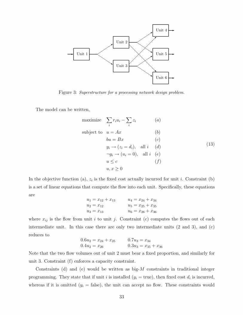
Unit 1- ��

��3

QQ

QQs

Unit 2 ��

��3

QQ

QQs

@@

@@

@@

@RUnit 3 �

��

�3

QQ

QQs

��

��

��

��

Unit 4 -

Unit 5 -

Unit 6 -

Figure 3: Superstructure for a processing network design problem.

The model can be written,

maximize∑

i

riui −∑

i

zi (a)

subject to u = Ax (b)

bu = Bx (c)

yi → (zi = di), all i (d)

¬yi → (ui = 0), all i (e)

u ≤ c (f)

u, x ≥ 0

(13)

In the objective function (a), zi is the fixed cost actually incurred for unit i. Constraint (b)

is a set of linear equations that compute the flow into each unit. Specifically, these equations

areu1 = x12 + x13 u4 = x24 + x34

u2 = x12 u5 = x25 + x35

u3 = x13 u6 = x26 + x36

where xij is the flow from unit i to unit j. Constraint (c) computes the flows out of each

intermediate unit. In this case there are only two intermediate units (2 and 3), and (c)

reduces to0.6u2 = x24 + x25 0.7u3 = x34

0.4u2 = x26 0.3u3 = x35 + x36

Note that the two flow volumes out of unit 2 must bear a fixed proportion, and similarly for

unit 3. Constraint (f) enforces a capacity constraint.

Constraints (d) and (e) would be written as big-M constraints in traditional integer

programming. They state that if unit i is installed (yi = true), then fixed cost di is incurred,

whereas if it is omitted (yi = false), the unit can accept no flow. These constraints would

33

in practice be replaced by inequality-or global constraints as discussed in Section 5.1.3, in

order to obtain the continuous relaxation described there.

One can accelerate the search by making some simple observations. It is clearly pointless

to install unit 1 unless one installs unit 2 or unit 3. This can be written

y1 → (y2 ∨ y3)

Similarly there is no point to installing unit 2 unless one installs units 1 and 6, or unless one

installs unit 4 or unit 5. Rules of this sort can be listed as follows and added to the model:

cnf

y1 → (y2 ∨ y3) y3 → y4

y2 → y1 y3 → (y5 ∨ y6)y2 → (y4 ∨ y5) y4 → (y2 ∨ y3)y2 → y6 y5 → (y2 ∨ y3)y3 → y1 y6 → (y2 ∨ y3)

(14)

These “don’t-be-stupid” rules are not implied by the original model, because they exclude

feasible solutions. There is nothing infeasible about installing a unit that is necessarily idle.

Yet computational experiments show (Grossmann et al. 1994) that without don’t-be-stupid

constraints, a branch-and-bound search (traditional or hybrid) can examine and reject a

large number of solutions in which useless units are installed.

A large number of don’t-be-stupid rules can be used when they are processed symbolically

rather than added to the relaxation. After one or more variables yi are fixed by branching,

logical inference methods can infer that other variables must be fixed, even in cases where

integer programming methods would not detect a fixed variable. This reduces the number

of solutions examined, which can be very useful in engineering design problems where the

continuous relaxation can be nonlinear and hard to solve. A global constraint “cnf” is used

in (14) to signal the solver to apply a logical inference procedure, such as the resolution

method.

A similar consideration applies to symmetry breaking rules, which can be used in some

problems to help avoid enumerating equivalent solutions. They can appear in large numbers

if processed symbolically.

5.3.2 Lot Sizing

A lot sizing problem discussed by Wolsey (1998) illustrates some of the considerations that

arise when designing a relaxation in the context of integrated modeling. (We modify the

example slightly.) Several products i must be shipped in specified quantities dit on each day

34

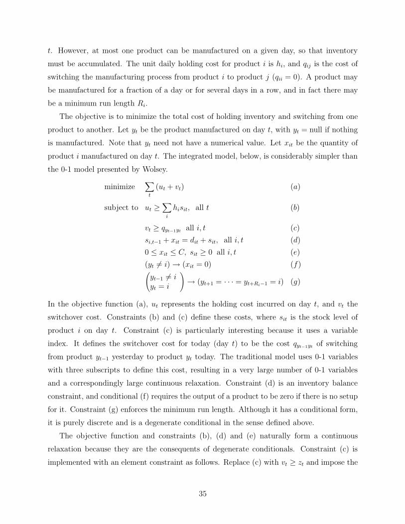
t. However, at most one product can be manufactured on a given day, so that inventory

must be accumulated. The unit daily holding cost for product i is hi, and qij is the cost of

switching the manufacturing process from product i to product j (qii = 0). A product may

be manufactured for a fraction of a day or for several days in a row, and in fact there may

be a minimum run length Ri.

The objective is to minimize the total cost of holding inventory and switching from one

product to another. Let yt be the product manufactured on day t, with yt = null if nothing

is manufactured. Note that yt need not have a numerical value. Let xit be the quantity of

product i manufactured on day t. The integrated model, below, is considerably simpler than

the 0-1 model presented by Wolsey.

minimize∑

t

(ut + vt) (a)

subject to ut ≥∑

i

hisit, all t (b)

vt ≥ qyt−1yt all i, t (c)

si,t−1 + xit = dit + sit, all i, t (d)

0 ≤ xit ≤ C, sit ≥ 0 all i, t (e)

(yt 6= i)→ (xit = 0) (f)(yt−1 6= iyt = i

)→ (yt+1 = · · · = yt+Ri−1 = i) (g)

In the objective function (a), ut represents the holding cost incurred on day t, and vt the

switchover cost. Constraints (b) and (c) define these costs, where sit is the stock level of

product i on day t. Constraint (c) is particularly interesting because it uses a variable

index. It defines the switchover cost for today (day t) to be the cost qyt−1yt of switching

from product yt−1 yesterday to product yt today. The traditional model uses 0-1 variables

with three subscripts to define this cost, resulting in a very large number of 0-1 variables

and a correspondingly large continuous relaxation. Constraint (d) is an inventory balance

constraint, and conditional (f) requires the output of a product to be zero if there is no setup

for it. Constraint (g) enforces the minimum run length. Although it has a conditional form,

it is purely discrete and is a degenerate conditional in the sense defined above.

The objective function and constraints (b), (d) and (e) naturally form a continuous

relaxation because they are the consequents of degenerate conditionals. Constraint (c) is

implemented with an element constraint as follows. Replace (c) with vt ≥ zt and impose the

35

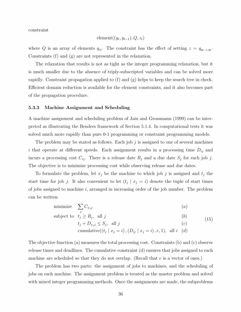
constraint

element((yt, yt−1), Q, zt)

where Q is an array of elements qij . The constraint has the effect of setting z = qyt−1,yt .

Constraints (f) and (g) are not represented in the relaxation.

The relaxation that results is not as tight as the integer programming relaxation, but it

is much smaller due to the absence of triply-subscripted variables and can be solved more

rapidly. Constraint propagation applied to (f) and (g) helps to keep the search tree in check.

Efficient domain reduction is available for the element constraints, and it also becomes part

of the propagation procedure.

5.3.3 Machine Assignment and Scheduling

A machine assignment and scheduling problem of Jain and Grossmann (1999) can be inter-

preted as illustrating the Benders framework of Section 5.1.4. In computational tests it was

solved much more rapidly than pure 0-1 programming or constraint programming models.

The problem may be stated as follows. Each job j is assigned to one of several machines

i that operate at different speeds. Each assignment results in a processing time Dij and

incurs a processing cost Cij. There is a release date Rj and a due date Sj for each job j.

The objective is to minimize processing cost while observing release and due dates.

To formulate the problem, let xj be the machine to which job j is assigned and tj the

start time for job j. It also convenient to let (tj | xj = i) denote the tuple of start times

of jobs assigned to machine i, arranged in increasing order of the job number. The problem

can be written

minimize∑j

Cxjj (a)

subject to tj ≥ Rj , all j (b)

tj + Dxjj ≤ Sj , all j (c)

cumulative((tj | xj = i) , (Dij | xj = i) , e, 1), all i (d)

(15)

The objective function (a) measures the total processing cost. Constraints (b) and (c) observe

release times and deadlines. The cumulative constraint (d) ensures that jobs assigned to each

machine are scheduled so that they do not overlap. (Recall that e is a vector of ones.)

The problem has two parts: the assignment of jobs to machines, and the scheduling of

jobs on each machine. The assignment problem is treated as the master problem and solved

with mixed integer programming methods. Once the assignments are made, the subproblems

36

are dispatched to a constraint programming solver to find a feasible schedule. If there is no

feasible schedule, a Benders cut is generated.

Variables x and t go into the master problem. Finite domain variables t′ that are linked

with t appear in the subproblem. The problem is therefore written as follows for Benders

decomposition.

minimize∑j

Cxjj (a)

subject to tj ≥ Rj , all j (b)

tj + Dxjj ≤ Sj , all j (c)

cumulative((

t′j | xj = i)

, (Dij | xj = i) , e, 1), all i (d)

t′j ≥ Rj , all j (e)

t′j + Dxjj ≤ Sj , all j (f)

link(t′j , tj), all j

(16)

The link constraint requires that Lj ≤ tj ≤ Uj , where Lj is the smallest and Uj the largest

time in the current domain of t′j.

If x has been fixed to x, the subproblem is

t′j ≥ Rj, all j

t′j + Dxjj ≤ Sj, all j

cumulative((

t′j | xj = i), (Dij | xj = i) , e, 1

), all i

(17)

The subproblem can be decomposed into smaller problems, one for each machine. If a smaller

problem is infeasible for some i, then the jobs assigned to machine i cannot all be scheduled

on that machine. In fact, going beyond Jain and Grossmann (1999), there may be a subset

J of these jobs that cannot be scheduled on machine i. This gives rise to a Benders cut

stating that at least one of the jobs in J must be assigned to another machine.

∨j∈J

(xj 6= i) (18)

Let xk be the solution of the kth master problem, Ik the set of machines i in the resulting

subproblem for which the schedule is infeasible, and Jki the infeasible subset. The master

problem can now be written,

minimize∑j

Cxjj

subject to tj ≥ Rj , all j

tj + Dxjj ≤ Sj, all j∨j∈Jki

(xj 6= i), i ∈ Ik, k = 1, . . . , K

(19)

37

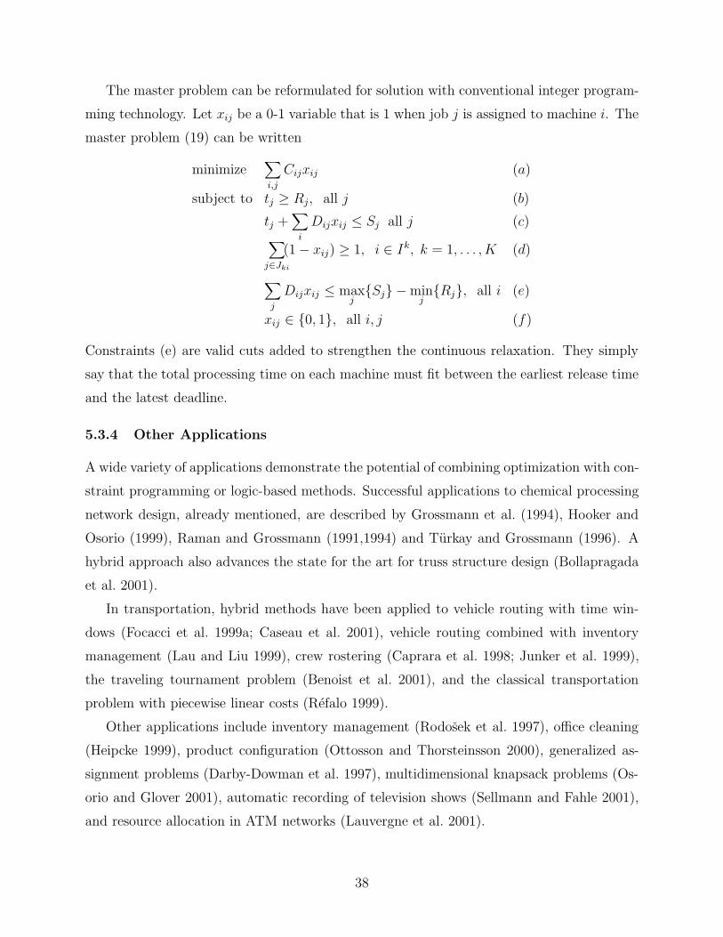
The master problem can be reformulated for solution with conventional integer program-

ming technology. Let xij be a 0-1 variable that is 1 when job j is assigned to machine i. The

master problem (19) can be written

minimize∑i,j

Cijxij (a)

subject to tj ≥ Rj, all j (b)

tj +∑

i

Dijxij ≤ Sj all j (c)∑j∈Jki

(1− xij) ≥ 1, i ∈ Ik, k = 1, . . . , K (d)

∑j

Dijxij ≤ maxj{Sj} −min

j{Rj}, all i (e)

xij ∈ {0, 1}, all i, j (f)

Constraints (e) are valid cuts added to strengthen the continuous relaxation. They simply

say that the total processing time on each machine must fit between the earliest release time

and the latest deadline.

5.3.4 Other Applications

A wide variety of applications demonstrate the potential of combining optimization with con-

straint programming or logic-based methods. Successful applications to chemical processing

network design, already mentioned, are described by Grossmann et al. (1994), Hooker and

Osorio (1999), Raman and Grossmann (1991,1994) and Turkay and Grossmann (1996). A

hybrid approach also advances the state for the art for truss structure design (Bollapragada

et al. 2001).

In transportation, hybrid methods have been applied to vehicle routing with time win-

dows (Focacci et al. 1999a; Caseau et al. 2001), vehicle routing combined with inventory

management (Lau and Liu 1999), crew rostering (Caprara et al. 1998; Junker et al. 1999),

the traveling tournament problem (Benoist et al. 2001), and the classical transportation

problem with piecewise linear costs (Refalo 1999).

Other applications include inventory management (Rodosek et al. 1997), office cleaning

(Heipcke 1999), product configuration (Ottosson and Thorsteinsson 2000), generalized as-

signment problems (Darby-Dowman et al. 1997), multidimensional knapsack problems (Os-

orio and Glover 2001), automatic recording of television shows (Sellmann and Fahle 2001),

and resource allocation in ATM networks (Lauvergne et al. 2001).

38

Most applications seem to have been to scheduling. These include machine schedul-

ing (Heipcke 1998; Raman and Grossmann 1993), sequencing with setups (Focacci et al.

1999), hoist scheduling (Rodosek and Wallace 1998), employee scheduling (Partouche 1998),

dynamic scheduling (El Sakkout et al. 1998), and lesson timetables (Focacci et al. 1999).

Production scheduling applications include scheduling with resource constraints (Pinto and

Grossmann 1997) and with labor resource constraints in particular (Heipcke 1999), two-

stage process scheduling (Jain and Grossmann 1999), machine allocation and scheduling

(Puget and Lustig 1999), production flow planning with machine assignment (Heipcke 1999),

scheduling with piecewise linear costs (Ottosson et al. 1999), scheduling with earliness and

tardiness costs (Beck 2001), and organization of a boat party (Hooker and Osorio 1999;

Smith et al. 1996).

These applications only begin to tap the potential of integrated methods. New ones are

appearing as this article is written.

6. Future Research

Several research needs surfaced in the course of the foregoing discussion. One might begin

with two broad research goals:

• Develop a robust and widely acceptable integration scheme for optimization and con-

straint programming. Perhaps the first step is to take the integrated modeling and

decomposition schemes (discussed earlier) deeper into practical applications to see how

they fare.

• Develop a generic modeling language that can serve as the basis for one or more

viable commercial products that integrate optimization and constraint programming.

The language should (a) strike a balance between the procedural and the declarative,

(b) indicate by its syntactic structure how optimization and constraint programming

should interact, and (c) allow the user to encode knowledge of problem structure, for

instance by using global constraints.

Some more specific research projects might also be mentioned.

• Combine integrated modeling and decomposition into a single framework.

39

• Develop a repertory of useful global constraints for each of several application domains.

They should succinctly capture characteristic modeling situations of the domain and

be amenable to logic processing and/or relaxation.

• Take advantage of the optimization community’s experience with continuous relax-

ations to develop such relaxations for constraint programming predicates.

• Explore discrete relaxations for constraint programming predicates, such as those based

on discrete relaxation duals.

• Move from the exclusive focus on domain reduction to other types of consistency main-

tenance as well. Rather than generate in-domain and other very simple constraints,

generate a wider variety of constraints that comprise tighter and yet soluble relaxations.

• Generalize the integer programming idea of a separating constraint to a broader con-

text.

There is something to be said for isolated research groups working in parallel. They may

develop complementary approaches that at some point can be profitably combined. This

seems to be the situation with optimization and constraint programming. Their ignorance

of each other over a period of years was perhaps a good thing. It is hard to pick the right

time for interaction to begin, but in any event it has begun.

References

Adams, W.P., P.M. Dearing. 1994. On the equivalence between roof duality and Lagrangean

duality for unconstrained 0-1 quadratic programming problems, Discrete Applied Math-

ematics 48 1-20.

Adams, W.P., A. Billionnet, A. Sutter. 1990. Unconstrained 0-1 optimization, and La-

grangean relaxation, Discrete Applied Mathematics 29 131-142.

Aggoun, A., M. Dincbas, A. Herold, H. Simonis, and P. Van Hentenryck. 1987. The CHIP

system. Technical Report TR-LP-24, European Computer Industry Research Centre

(ECRC) (Munich, Germany).

Arnborg, S., D. G. Corneil, A. Proskurowski. 1987. Complexity of finding embeddings in a

k-tree, SIAM Journal on Algebraic and Discrete Mathematics 8 277-284.

40

Arnborg, S., and A. Proskurowski. 1986. Characterization and recognition of partial k-trees,

SIAM Journal on Algebraic and Discrete Mathematics 7 305-314.

Balas, E. 1974. Intersection cuts from disjunctive constraints, Management Sciences Re-

search Report No. 330, Graduate School of Industrial Administration, Carnegie Mellon

University.

Balas, E. 1975. Disjunctive programming: Cutting planes from logical conditions, in O.

L. Mangasarian, R. R. Meyer, and S. M. Robinson, eds., Nonlinear Programming 2,

Academic Press (New York) 279-312.

Balas, E. 1977. A note on duality in disjunctive programming, Journal of Optimization

Theory and Applications 21 523-527.

Balas, E., Disjunctive programming, Annals Discrete Mathematics 5 (1979) 3-51.

Balas, E., S. Ceria, G. Cornuejols. 1996. Mixed 0-1 programming by lift-and-project in a

branch and cut framework, Management Science 42 1229-1246.

Balas, E., R. Jeroslow. 1972. Canonical cuts on the unit hypercube, SIAM Journal on

Applied Mathematics 23 61-69.

Balas, E., J. B. Mazzola. 1980a. Nonlinear 0-1 programming: I. Linearization Techniques,

Mathematical Programming 30 1-20.

Balas, E., and J. B. Mazzola. 1980b. Nonlinear 0-1 programming: II. Dominance relations

and algorithms, Mathematical Programming 30 22-45.

Barth, P. 1995. Logic-Based 0-1 Constraint Solving in Constraint Logic Programming,

Kluwer (Dordrecht). The system OPBDP is available at http://ww.mpi-sb.mpg.de/units/

ag2/software/opbdp.

Beaumont, N. 1990. An algorithm for disjunctive programs, European Journal of Operational

Research 48 362-371.

Beck, C. 2001. A hybrid approach to scheduling with earliness and tardiness costs, Third In-

ternational Workshop on Integration of AI and OR Techniques (CPAIOR01), http://www-

icparc.doc.ic.ac.uk/cpAIOR01.

Benders, J. F. 1962. Partitioning procedures for solving mixed-variables programming prob-

lems, Numerische Mathematik 4 238-252.

Bennaceur, H., I. Gouachi, G. Plateau. 1998. An incremental branch-and-bound method

41

for the satisfiability problem, INFORMS Journal on Computing 10 301-308.

Benoist, T., F. Laburthe, B. Rottembourg. 2001. Lagrange relaxation and constraint

programming collaborative schemes for travelling tournament problems, Third Interna-

tional Workshop on Integration of AI and OR Techniques (CPAIOR01), http://www-

icparc.doc.ic.ac.uk/cpAIOR01.

Berge, C. 1970. Graphes et hypergraphes, Dunod (Paris).

Beringer, H., B. De Backer. 1995. Combinatorial problem solving in constraint logic

programming with cooperating solvers, in C. Beierle and L. Pl”umer, eds., Logic Pro-

gramming: Formal Methods and Practical Applications, Elsevier/North-Holland (Ams-

terdam), 245-272.

Bertele, U., F. Brioschi. 1972. Nonserial Dynamic Programming, Academic Press (New

York).

Blair, C. E., R. G. Jeroslow, J. K. Lowe. 1988. Some results and experiments in programming

techniques for propositional logic, Computers and Operations Research 13 633-645.

Bockmayr, A., T. Kasper. 1998. Branch and infer: A unifying framework for integer and

finite domain constraint programming, INFORMS Journal on Computing 10 287-300.

Boole, G. 1847. The Mathematical Analysis of Logic: Being a Essay Toward a Calculus of

Deductive Reasoning, Blackwell (Oxford, 1951), original work published 1847.

Boole, G. 1952. Studies in Logic and Probability, in R. Rhees, ed., Watts, and Company

(London) and Open Court Publishing Company (La Salle, Illinois). This ia a collection

of some of Boole’s papers.

Bollapragada, S., O. Ghattas, J. N. Hooker. 2001. Optimal design of truss structures by

mixed logical and linear programming, Operations Research, to appear.

Cagan, J., I. E. Grossmann, J. N. Hooker. 1997. A conceptual framework for combining

artificial intelligence and optimization in engineering design, Research in Engineering

Design 9 20-34.

Caprara, A., et al. 1998. Integrating constraint logic programming and operations research

techniques for the crew rostering problem, Software - Practice and Experience 28 49-76.

Caseau, Y., G. Silverstein, F. Laburthe. 2001. Learning hybrid algorithms for vehicle

routing problems, Third International Workshop on Integration of AI and OR Techniques

42

(CPAIOR01), http://www-icparc.doc.ic.ac.uk/cpAIOR01.

Chandrasekaran, R. 1984. Integer programming problems for which a simple type of rounding

algorithm works, in W. R. Pulleyblank, ed., Progress in Combinatorial Optimization,

Academic Press Canada, 101-106.

Chandru, V., J. N. Hooker. 1991. Extended Horn sets in propositional logic, Journal of the

ACM 38 205-221.

Chandru, V., J. N. Hooker. 1999. Optimization Methods for Logical Inference, Wiley (New

York).

Chhajed, D., T. J. Lowe. 1994. Solving structured multifacility location problems efficiently,

Transportation Science 28 104-115.

Clocksin, W. F., C. S. Mellish. 1984. Programming in Prolog, 2nd ed., Springer (New York).

Colmerauer, A. 1982. PROLOG II reference maual and theoretical model. Technical report,

Groupe Intelligence Artificielle, Universite Aix-Marseille II (October).

Colmerauer, A. 1987. Opening the PROLOG-III universe, BYTE Magazine 12 no. 9 (Au-

gust).

Colmerauer, A. 1990. An introduction to PROLOG-III, Communications of the ACM 33

no. 7, 69-90.

Colmerauer, A. 1996. Specifications de Prolog IV, Technical report, Laboratoire d’Informatique

de Marseille, Universite Aix-Marseille II.

Crama, Y., P. Hansen, and B. Jaumard. 1990. The basic algorithm for pseudo-boolean

programming revisited, Discrete Applied Mathematics 29 171-185.

Darby-Dowman, K., J. Little. 1998. Properties of some combinatorial optimization prob-

lems and their effect on the performance of integer programming and constraint logic

programming, INFORMS Journal on Computing 10 276-286.

Darby-Dowman, K., J. Little, G. Mitra, M. Zaffalon. 1997. Constraint logic programming

and integer programming approaches and their collaboration in solving an assignment

scheduling problem, Constraints 1 245-264.

De Farias, I. R., E. L. Johnson and G. L. Nemhauser. 1999. A branch-and-cut approach

without binary variables to combinatorial optimization problems with continuous vari-

ables and combinatorial constraints, manuscript, Georgia Institute of Technology.

43

Dechter, R. 1999. Bucket elimination: A unifying framework for reasoning, Artificial Intel-

ligence 41 41-85.

Dechter, R. 2000. An anytime approximation for optimizing policies under uncertainty,

presented in Workshop on Decision Theoretic Planning, AIPS2000.

Dechter, R., J. Pearl. 1988. Tree-clustering schemes for constraint processing, Proceeedings,

National Conference on Artificial Intelligence, AAAI 150-154.

Dincbas, M., P. Van Hentenryck, H. Simonis, A. Aggoun, T. Graf, F. Bertier. 1988. The

constraint programming language CHIP, Proceedings on the International Conference on

Fifth Generation Computer Systems, Tokyo (December).

El Sakkout, L., T. Richards, M. Wallace. 1998. Minimal perturbance in dynamic scheduling,

in H. Prade, ed., Proceedings, 13th European Conference on Artificial Intelligence, Wiley

(New York), 504-508.

Focacci, F., A. Lodi, M. Milano. 1999. Cost-based domain filtering, Principles and Practice

of Constraint Programming, Lecture Notes in Computer Science 1713 189-203.

Focacci, F., A. Lodi, M. Milano. 1999a. Solving TSP with time windows with constraints,

presented at 16th International Conference on Logic Programming, (Las Cruces, NM).

Fortet, R. 1959. L’algebre de Boole et ses applications en recherche operation-nelle, Cahiers

du centre d’etudes de recherche operationnelle 1 5-36.

Fortet, R. 1960. Applications de l’algebre de Boole en recherche operation-nelle, Revue

Fran caise d’informatique et de recherche operationnelle 1 17-25.

Freuder, E. C. 1982. A sufficient condition for backtrack-free search, Journal of the ACM

29 24-32.

Garfinkel, R., G. Nemhauser. 1970. Optimal political districting by implicit enumeration

techniques, Management Science 16 B495-B508.

Gaschnig, J. 1977. A general backtrack algorithm that eliminates most redundant tests,

Proceedings, 5th International Joint Conference on AI 457.

Gaschnig, J. 1978. Experimental studies of backtrack vs. Waltz-type vs. new algorithms for

satisficing-assignment problems, Proceedings, 2nd National Conference of the Canadian

Society for Computational Studies of Intelligence, 19-21.

Geoffrion, A. M. 1972. Generalized Benders decomposition, Journal of Optimization Theory

44

and Applications 10 237-260.

Ginsberg, M. L. 1993. Dynamic backtracking, Journal of Artificial Intelligence Research 1

25-46.

Ginsberg, M. L., and D. A. McAllester. 1994. GSAT and dynamic backtracking, Second

Workshop on Principles and Practice of Constraint Programming (May) 216-225.

Glover, F. 1975. Surrogate constraint duality in mathematical programming, Operations

Research 23 434-451.

Gomory, R. E. 1965. On the relation between integer and noninteger solutions to linear

programs, Proceedings of the National Academy of Sciences of the USA 53 260-265.

Granot, F., P. L. Hammer. 1971. On the use of boolean functions in 0-1 programming,

Methods of Operations Research 12 154-184.

Granot, F., P. L. Hammer. 1975. On the role of generalized covering problems, Cahiers du

Centre d’Etudes de Recherche Operationnelle 17 277-289.

Grossmann, I. E., J. N. Hooker, R. Raman, H. Yan. 1994. Logic cuts for processing networks

with fixed charges, Computers and Operations Research 21 265-279.

Gurari, E., I. Sudborough. 1984. Improved dynamic programming algorithms for bandwidth

minimization and the mincut linear arrangement problem, Journal of Algorithms 5 531-

546.

Hailperin, T. 1976. Boole’s Logic and Probability, Studies in Logic and the Foundations of

Mathematics v. 85, North-Holland.

Hailperin, T. 1986. Boole’s Logic and Probability, Second Edition, Studies in Logic and the

Foundations of Mathematics v. 85, North-Holland.

Hammer, P. L., P. Hansen, B. Simeone. 1984. Roof duality, complementation and persistency

in quadratic 0-1 optimization, Mathematical Programming 28 121-155.

Hammer, P. L., U. Peled. 1972. On the maximization of a pseudo-boolean function, Journal

of the Assosciation for Computing Machinery 19 265-282.

Hammer, P. L., I. Rosenberg, S. Rudeanu. 1963. On the determination of the minima of

pseudo-boolean functions (in Romanian), Studii si Cercetari Matematice 14 359-364.

Hammer, P. L., S. Rudeanu. 1968. Boolean Methods in Operations Research and Related

Areas, Springer (New York).

45

Hansen, P. 1969. Un algorithme S.E.P. pour les programmes pseudo-booleens non lineaires,

Cahiers du Centre d’Etudes de Recherche Operationnelle 11 26-44.

Hansen, P. 1970. Un algorithme pour les programmes non lineaires en variables zero-un,

Comptes Rendus de l’Academie des Sciences de Paris 273 1700-1702.

Hansen, P. L., B. Jaumard, V. Mathon. 1993. Constrained nonlinear 0-1 programming,

ORSA Journal on Computing 5 97-119.

Hansen, P., S. H. Lu, B. Simeone. 1984. On the equivalence of paved duality and standard

linearization in nonlinear 0-1 optimization, Mathematical Programming 28 121-155.

Heipcke, S. 1998. Integrating constraint programming techniques into mathematical pro-

gramming, in H. Prade, ed., Proceedings, 13th European Conference on Artificial Intelli-

gence, Wiley (New York) 259-260.

Heipcke, S. 1999. Combined Modelling and Problem Solving in Mathematical Programming

and Constraint Programming, Ph.D. Thesis, University of Buckingham.

Hooker, J. N. 1988. Generalized resolution and cutting planes, Annals of Operations Research

12 217-239.

Hooker, J. N. 1989. Input proofs and rank one cutting planes, ORSA Journal on Computing

1 137-145.

Hooker, J. N. 1992. Generalized resolution for 0-1 linear inequalities, Annals of Mathematics

and Artificial Intelligence 6 271-286.

Hooker, J. N. 1994. Logic-based methods for optimization, in A. Borning, ed., Principles and

Practice of Constraint Programming, Lecture Notes in Computer Science 874 336-349.

Hooker, J. N. 1995. Logic-based Benders decomposition, presented at INFORMS 1995.

Hooker, J. N. 1997. Constraint satisfaction methods for generating valid cuts, in D. L.

Woodruff, ed., Advances in Computational and Stochasic Optimization, Logic Program-

ming and Heuristic Search, Kluwer (Dordrecht) 1-30.

Hooker, J. N. 2000. Logic-Based Methods for Optimization: Combining Optimization and

Constraint Satisfaction, Wiley (New York).

Hooker, J. N. 2001. Integrating solution methods for optimization and constraint satisfaction

problems, manuscript, Carnegie Mellon University, 2001.

Hooker, J. N., C. Fedjki. 1990. Branch-and-cut solution of inference problems in proposi-

46

tional logic, Annals of Mathematics and Artificial Intelligence 1 123-140.

Hooker, J. N., Hak-Jin Kim, G. Ottosson. 2001. A declarative modeling framework that

combines solution methods, Annals of Operations Research, to appear.

Hooker, J. N., M. A. Osorio. 1999. Mixed logical/linear programming, Discrete Applied

Mathematics 96-97 395-442.

Hooker, J. N. G. Ottosson. 1998. Logic-based Benders decomposition, manuscript, Carnegie

Mellon University.

Hooker, J. N., G. Ottosson, E. Thorsteinsson, Hak-Jin Kim. 1999. On integrating constraint

propagation and linear programming for combinatorial optimization, Proceeedings, 16th

National Conference on Artificial Intelligence, MIT Press (Cambridge) 136-141.

Hooker, J. N., G. Ottosson, E. Thorsteinsson, Hak-Jin Kim. 2000. A scheme for unifying

optimization and constraint satisfaction methods, Knowledge Engineering Review 15 11-

30.

Hooker, J. N., and Hong Yan. 1995. Logic circuit verification by Benders decomposition,

in V. Saraswat and P. Van Hentenryck, eds., Principles and Practice of Constraint Pro-

gramming: The Newport Papers, MIT Press (Cambridge, MA) 267-288.

Jaffar, J., J.-L. Lassez. 1987. Constraint logic programming, Proceedings, 14th ACM Sym-

posium on Principles of Programming Languages, ACM Press (Munich) 111-119.

Jaffar, J., S. Michaylov. 1987. Methodology and implementation of a CLP system, in J.-L.

Lassez, ed., Logic Programming: Proceedings, 4th International Conference, MIT Press

(Cambridge) 196-218.

Jaffar, J., S. Michaylov, P. Stuckey, R. Yap. 1992. The CLP(<) language and system, ACM

Transactions of Programming Languages and Systems 14 339-395.

Jaffar, J., P. Stuckey. 1986. Semantics of infinite tree logic programming, Theoretical Com-

puter Science 42 141-158.

Jain, V., I. E. Grossmann. 1999. Algorithms for hybrid MILP/CLP models for a class of

optimization problems, INFORMS Journal on Computing, to appear.

Jeroslow, R. E. 1987. Representability in mixed integer programming, I: Characterization

results, Discrete Applied Mathematics 17 223-243.

Jeroslow, R. E. 1989. Logic-Based Decision Support: Mixed Integer Model Formulation,

47

Annals of Discrete Mathematics 40. North-Holland (Amsterdam).

Jeroslow, R. E., R. K. Martin, R. L. Rardin, J. Wang. 1989. Gain-free Leontief flow

problems, mauscript, Graduate School of Business, University of Chicago.

Jeroslow, R. G., J. Wang. 1989. Dynamic programming, integral polyhedra and Horn clause

knowledge base, ORSA Journal on Computing 4 7-19.

Junker, U., S. E. Karisch, N. Kohl, B. Vaaben, T. Fahle, M. Sellmann. 1999. A framework

for constraint programming based column generation, in J. Jaffar, ed., Principles and

Practice of Constraint Programming, Lecture Notes in Computer Science 1713, Springer

(Berlin), 261-274.

Kim, Hak-Jin, J. N. Hooker. 2001. Solving fixed-charge network flow problems with a

hybrid optimization and constraint programming approach, manuscript, Carnegie Mellon

UNiversity.

Kowalski, R. 1979. Logic for Problem Solving, Elsevier North-Holland (New York).

Lau, H. C., Q. Z. Liu. 1999. Collaborative model and algorithms for supporting real-time

distribution logistics systems, CP99 post-Conference Workshop on Large Scale Combina-

torial Optimization and Constraints, http://www.dash.co.uk/wscp99, 30-44.

Laundy, R. S. 1986. Logically Constrained Mathematical Programming Problems, Ph.D.

thesis, University of Southampton.

Lauritzen, S. L., D. J. Spiegelhalter. 1988. Local computations with probabilities on graph-

ical structures and their application to expert systems, Journal of the Royal Statistical

Society B, 50 157-224.

Lauvergne, M., P. David, P. Boizumault. 2001. Resource allocation in ATM networks:

A hybrid approach, Third International Workshop on the Integration of AI and OR

Techniques (CPAIOR 2001), http://www-icparc.doc.ic.ac.uk/cpAIOR01/.

Little, J., K. Darby-Dowman. 1995. The significance of constraint logic programming to

operational research, in M. Lawrence and C. Wilson, eds., Operational Research 20-45.

Lloyd, W. 1984. Foundations of Logic Programming, Springer (New York).

Lu, S. H., A. C. Williams. 1987. Roof duality for polynomial 0-1 optimization, Mathematical

Programming 37 357-360.

Marriott, K., P. J. Stuckey. 1998. Programming with Constraints: An Introduction, MIT

48

Press (Cambridge).

McAllester, D. A. 1993. Partial order backtracking, Manuscript, AI Laboratory, MIT, Cam-

bridge.

McAloon, K., C. Tretkoff. 1996. Optimization and Computational Logic, Wiley (New York).

The system 2LP is available at http:// www.sci.brooklyn.cuny.edu/ lbslab/doc lplp.html.

Oplobedu, A., J. Marcovitch, Y. Tourbier. 1989. Charme: Un langage industriel de program-

mation par constraintes, illustre par une application chez renault, in Ninth International

Workshop on Expert Systems and Their Applications: General Conference 1 (EC2) 55-70.

Osorio, M. A., F. Glover. 2001. Logic cuts using surrogate constraint analysis in the multi-

dimensional knapsack problem, Third International Workshop on Integration of AI and

OR Techniques (CPAIOR01), http://www-icparc.doc.ic.ac.uk/cpAIOR01.

Osorio, M. A., J. N. Hooker. 1996. General mixed logical/linear solver, presented at IN-

FORMS National Meeting, Washington, D.C. (April).

Ottosson, G., E. Thorsteinsson. 2000. Linear relaxations and reduced-cost based propa-

gation of continuous variable subscripts, presented at Second International Workshop

on Integration of AI and OR Techniques in Constraint Programming for Combinatorial

Optimization Problems, University of Paderborn.

Ottosson, G., E. Thorsteinsson, J. N. Hooker. 1999. Mixed global constraints and inference

in hybrid CLP-IP solvers, CP99 Post-Conference Workshop on Large Scale Combinatorial

Optimization and Constraints, http://www.dash.co.uk/wscp99, 57-78.

Partouche, A. 1998. Planification d’horaires de travail, Ph.D. thesis, Universite Paris-

Daphine, U. F. R. Sciences des Organisations.

Pinto, J. M., I. E. Grossmann. 1997. A logic-based approach to scheduling problems with

resource constraints, Computers and Chemical Engineering 21 801-818.

Puget, J.-F. 1992. PECOS: A high-level constraint programming language, in Proceedings,

SPICIS’92 (Singapore).

Puget, J.-F. 1994. A C++ implementation of CLP, in Proceedings of SPICIS’94 (Singapore).

Puget, J.-F., M. Leconte. 1995. Beyond the black box: Constraints as objects, in J. Lloyd,

ed., Logic Programming: Proceedings, 1988 Joint International Conference and Sympo-

sium, MIT Press (Cambridge) 140-159.

49

Puget, J.-F., I. Lustig. 1999. Constraint programming and math programming, Manuscript,

ILOG S. A.

Quine, W. V. 1952. The problem of simplifying truth functions, American Mathematical

Monthly 59 521-531.

Quine, W. V. 1955. A way to simplify truth functions, American Mathematical Monthly 62

627-631.

Raman, R., I. Grossmann. 1991. Symbolic integration of logic in min mixed-integer linear

programming techniques for process synthesis, Computers and Chemical Engineering 17

909-927.

Raman, R., I. Grossmann. 1993. Relation between MILP modeling and logical inference for

chemical process synthesis, Computers and Chemical Engineering 15 73-84.

Raman, R., I. Grossmann. 1994. Modeling and computational techniques for logic based

integer programming, Computers and Chemical Engineering 18 563-578.

Refalo, P. 1999. Tight cooperation and its application in piecewise linear optimization,

in J. Jaffar, ed., Principles and Practice of Constraint Programming, Lecture Notes in

Computer Science 1713, Springer (Berlin), 373-389.

Regin, J.-C. 1994. A filtering algorithm for constraints of difference in CSPs, Proceedings,

National Conference on Artificial Intelligence 362-367.

Rodosek, R., M. Wallace. 1998. A generic model and hybrid algorithm for hoist scheduling

problems, Principles and Practice of Constraint Programming (CP-98), Lecture Notes in

Computer Science 1520, Springer (Berlin) 385-399.

Rodosek, R., M. Wallace, M. Hajian. 1997. A new approach to integrating mixed integer

programming and constraint logic programming, Annals of Operations Research 86 63-87.

Saxe, J. 1980. Dynamic programming algorithms for recognizing small bandwidth graphs in

polynomial time, SIAM Journal on Algebraic and Discrete Methods 1 363-369.

Schlipf, J. S., F. S. Annexstein, J. V. Franco, R. P. Swaminathan. 1995. On finding solutions

for extended Horn formulas, University of Cincinnati.

Schaefer, T. J. 1978. The complexity of satisfiability problems, Proceedings, 10th ACM

Symposium on Theory of Computing, 216-226.

Sellmann, M., T. Fahle. 2001. CP-based Lagrangian relaxation for a multimedi application.

50

Third International Workshop on the Integration of AI and OR Techniques (CPAIOR

2001), http://www-icparc.doc.ic.ac.uk/cpAIOR01/.

Shafer, G., P. P. Shenoy, K. Mellouli. 1987. Propagating belief functions in qualitative

Markov trees, International Journal of Approximate Reasoning 1 349-400.

Smith, B. M., S. C. Brailsford, P. M. Hubbard, H. P. Williams. 1996. The progressive party

problem: Integer linear programming and constraint programming compared, Constraints

1 119-138.

Solnon, C. 1997. Cooperation de solveurs lineaires sur les reels pour la resolution de

problemes lineaires en nombres entiers, Journees Francophones de la programmation

logique par contraintes, Orleans, Hermes.

Sterling, L., E. Shapiro. 1986. The Art of Prolog: Advanced Programming Techniques, MIT

Press (Cambridge).

Thorsteinsson, E. S. 2001. Branch-and-check: A hybrid framework integrating mixed integer

programming and constraint logic programming, Seventh International Conference on

Principles and Practice of Constraint Programming (CP2001).

Tsang, E. 1993. Foundations of Constraint Satisfaction, Academic Press (London). Now

available from the author.

Turkay, M., I. E. Grossmann. 1996. Logic-based MINLP algorithms for the optimal synthesis

of process networks, Computers and Chemical Engineering 20 959-978.

Van Hentenryck, P. 1989. Constraint Satisfaction in Logic Programming, MIT Press (Cam-

bridge).

Van Hentenryck, P. 1999. Modeling with OPL Studio CHECK THIS, MIT Press (Cambridge,

MA).

Van Hentenryck, P., L. Michel. 1997. Newton: Constraint programming over nonlinear real

constraints, Technical Report CS-95-25, Computer Science Department, Brown Univer-

sity.

Van Hentenryck, P., L. Michel, F. Benhamou. 1998. Newton: Constraint programming over

nonlinear constraints, Science of Computer Programming 30 83-118.

Wallace, M., S. Novello, J. Schimpf. 1997. ECLiPSe: A platform for constraint logic pro-

gramming, ICL Systems Journal 12 159-200.

51

Williams, H. P. 1976. Fourier-Motzkin elimination extension to integer programming prob-

lems, Journal of Combinatorial Theory 21 118-123.

Williams, H. P. 1977. Logical problems and integer programming, Bulletin of the Institute

of Mathematics and its Implications 13 18-20.

Williams, H. P. 1987. Linear and integer programming applied to the propositional calculus,

International Journal of Systems Research and Information Science 2 81-100.

Williams, H. P. 1991. Computational logic and integer programming: Connections between

the methods of logic, AI and OR, Technical Report, University of Southamption.

Williams, H. P. 1995. Logic applied to integer programming and integer programming ap-

plied to logic, European Journal of Operations Research 81 605-616.

Williams, H. P., Hong Yan. 2001. Representations of the all-different predicate, INFORMS

Journal on Computing, to appear.

Williams, H. P., Hong Yan. 2001a. Convex hull representations of the at-least predicate of

constraint satisfaction, manuscript, London School of Economics.

Williams, H. P., J. M. Wilson. 1998. Connections between integer linear programming and

constraint logic programming-An overview and introduction to the cluster of articles,

INFORMS Journal on Computing 10 261-264.

Wilson, J. M. 1990. Compact normal forms in propositional logic and integer programming

formulations, Computers and Operations Research 90 309-314.

Wilson, J. M. 1995. Problem specification in constraint logic programming and integer pro-

gramming, Working paper 1995:32, Loughborough University Business School Research

Series.

Wilson, J. M. 1996. A note on logic cuts and valid inequalities for certain standard (0-1)

integer programs, JORBEL 36 27-41.

Wolsey, L. A. 1998. Integer Programming, Wiley (New York).

Yan, H., J. N. Hooker. 1999. Tight representation of logical constraints as cardinality rules,

Mathematical Programming 85 363-377.

Zabih, R. 1990. Some applications of graph bandwidth to constraint satisfaction problems,

Proceedings, National Conference on Artificial Intelligence, 46-51.

52