1

A LONG MEMORYPATTERN MODELLING AND RECOGNITION SYSTEM

FOR FINANCIAL TIME-SERIES FORECASTING

Sameer Singh

{s.singh@exeter.ac.uk}

University of ExeterDepartment of Computer Science

Prince of Wales RoadExeter EX4 4PT

Singh, S. "A Long Memory Pattern Modelling and Recognition System for Financial Forecasting",Pattern Analysis and Applications, vol. 2, issue 3, pp. 264-273, 1999.

2

A LONG MEMORYPATTERN RECOGNITION AND MODELLING SYSTEM

FOR FINANCIAL TIME-SERIES FORECASTING

ABSTRACT

In this paper, the concept of a long memory system for forecasting is developed.

Pattern Modelling and Recognition Systems are introduced as local

approximation tools for forecasting. Such systems are used for matching current

state of the time-series with past states to make a forecast. In the past, this system

has been successfully used for forecasting the Santa Fe competition data. In this

paper, we forecast the financial indices of six different countries and compare the

results with neural networks on five different error measures. The results show

that pattern recognition based approaches in time-series forecasting are highly

accurate and these are able to match the performance of advanced methods such

as neural networks.

3

1. MOTIVATION

Time-series forecasting is an important research area in several domains.

Traditionally, forecasting research and practice has been dominated by statistical

methods. More recently, neural networks and other advanced methods on

prediction have been used in financial domains [1-3]. As we get to know more

about the dynamic nature of the financial markets, the weaknesses of traditional

methods become apparent. In the last few years, research has focussed on

understanding the nature of financial markets before applying methods of

forecasting in domains including stock markets, financial indices, bonds,

currencies and varying types of investments. Peters [4] notes that most financial

markets are not Gaussian in nature and tend to have sharper peaks and fat tails, a

phenomenon well know in practice. In the face of such evidence, a number of

traditional methods based on Gaussian normality assumption have limitations

making accurate forecasts.

One of the key observations explained by Peters [4] is the fact that most financial

markets have a very long memory; what happens today affects the future forever.

In other words, current data is correlated with all past data to varying degrees.

This long memory component of the market can not be adequately explained by

systems that work with short-memory parameters. Short-memory systems are

characterised by using the use of last i series values for making the forecast in

univariate analysis. For example most statistical methods and neural networks are

given last i observations for predicting the actual at time i+1. For the sake of

4

argument, such systems are termed as ‘short memory systems’ in this paper.

Long memory systems on the other hand are characterised by their ability to

remember events in the long history of time-series data and their ability to make

decisions on the basis of such memories. Such a system is not constrained by how

old the memory is. Hence, in such systems the forecasts are based on historical

matches of market situations.

One strand of our motivation comes from the Fractal Market Hypothesis, Peters

[4]. Peters [4] provided extensive results supporting his claim that markets have a

fractal structure based on different investment horizons and that they cover more

distance than the square root of time, i.e. they are not random in nature. Instead

they consist of non-periodical cycles which are hard to detect and use in statistical

or neural forecasting. He argues that financial markets are predictable but

algorithms need long memories for accuracy in forecasting. The investment

behaviour in markets has a repetitive nature over a long period of time and we

believe that this can be detected using local approximation. Short memory

systems can not capture the essence of this behaviour. This paper is also

motivated by a study by Farmer and Sidorowich [5] who found that chaotic time-

series prediction is several orders of magnitude better using local approximation

techniques than universal approximators. Local approximation refers to the

concept of breaking up the time domain into several small neighbourhood regions

and analysing these separately. The well-known methods of local approximation

for time-series prediction include chart representations, nearest neighbour

5

methods [5] and pattern imitation techniques [6]. In this paper, we propose a new

method of local approximation based on pattern matching that will be

implemented in our Pattern Modelling and Recognition system.

A Pattern Modelling and Recognition System (PMRS) is a pattern recognition

tool for forecasting. In this paper we approach the development of this tool with

the aim of forecasting six different financial indices. The paper is organised as

follows. We first discuss the concept of local approximation in forecasting and

detail its implementation in the PMRS algorithm. The PMRS algorithm for

forecasting is detailed next. The paper discusses the financial index data used in

this study with their statistical characteristics. The results section compares the

results obtained using the PMRS algorithm and backpropagation neural networks

that are widely used in the financial industry. The results are compared on a total

of five different error measures. Plots comparing PMRS and neural network

predictions and actual series values for August 1996 are shown in Appendix I.

The paper concludes by suggesting further areas of improvement.

2. LOCAL APPROXIMATION USING PMRS

The main emphasis of local approximation techniques is to model the current state

of the time-series by matching its current state with past states. If we choose to

represent a time-series as y = {y1, y2, ... yn}, then the current state of size one of

the time-series is represented by its current value yn. One simple method of

prediction can be based on identifying the closest neighbour of yn in the past data,

say yj, and predicting yn+1 on the basis of yj+1. This approach can be modified by

6

calculating an average prediction based on more than one nearest neighbours. The

definition of the current state of a time-series can be extended to include more

than one value, e.g. the current state sc of size two may be defined as {yn-1, yn}.

For such a current state, the prediction will depend on the past state sp {yj-1, yj}

and next series value y+p given by yj+1, provided that we establish that the state

{yj-1, yj} is the nearest neighbour of the state {yj-1, yj} using some similarity

measurement. In this paper, we also refer to states as patterns. In theory, we can

have a current state of any size but in practice only matching current states of

optimal size to past states of the same size yields accurate forecasts since too

small or too large neighbourhoods do not generalise well. The optimal state size

must be determined experimentally on the basis of achieving minimal errors on

standard measures through an iterative procedure.

We can formalise the prediction procedure as follows:

ÿ = φ(sc, sp, y+

p, k, c)

where ÿ is the prediction for the next time step, sc is the current state, sp is the

nearest past state, y+p is the series value following past state sp, k is the state size

and c is the matching constraint. Here ÿ is a real value, sc or sp can be represented

as a set of real values, k is a constant representing the number of values in each

state, i.e. size of the set, and c is a constraint which is user defined for the

matching process. We define c as the condition of matching operation that series

direction change for each member in sc and sp is the same.

7

In order to illustrate the matching process for series prediction further, consider

the time series as a vector y = {y1, y2, ... yn} where n is the total number of points

in the series. Often, we also represent such a series as a function of time, e.g. yn =

yt, yn-1 = yt-1, and so on. A segment in the series is defined as a difference vector δδδδ

= (δ1, δ2, ... δn-1) where δi = yi+1 - yi, ∀ i, 1≤i≤n-1. A pattern contains one or more

segments and it can be visualised as a string of segments ρ = (δi, δi+1, ... δh) for

given values of i and h, 1≤i,h≤n-1, provided that h>i. In order to define any

pattern mathematically, we choose to tag the time series y with a vector of change

in direction. For this purpose, a value yi is tagged with a 0 if yi+1 < yi, and as a 1 if

yi+1 ≥ yi. Formally, a pattern in the time-series is represented as ρ = (bi, bi+1, ... bh)

where b is a binary value.

The complete time-series is tagged as (b1, ...bn-1). For a total of k segments in a

pattern, it is tagged with a string of k b values. For a pattern of size k, the total

number of binary patterns (shapes) possible is 2k. The technique of matching

structural primitives is based on the premise that the past repeats itself. Farmer

and Sidorowich [5] state that the dynamic behaviour of time-series can be

efficiently predicted by using local approximation. For this purpose, a map

between current states and the nearest neighbour past states can be generated for

forecasting.

Pattern matching in the context of time-series forecasting refers to the process

of matching current state of the time series with its past states. Consider the

8

tagged time series (b1, bi, ... bn-1). Suppose that we are at time n (yn) trying to

predict yn+1. A pattern of size k is first formulated from the last k tag values in the

series, ρ’ = (bn-k, ... bn-1). The size k of the structural primitive (pattern) used for

matching has a direct effect on the prediction accuracy. Thus the pattern size k

must be optimised for obtaining the best results. For this k is increased in every

trial by one unit till it reaches a predefined maximum allowed for the experiment

and the error measures are noted; the value of k that gives the least error is finally

selected. The aim of a pattern matching algorithm is to find the closest match of

ρ’ in the historical data (estimation period) and use this for predicting yn+1. The

magnitude and direction of prediction depend on the match found. The success in

correctly predicting series depends directly on the pattern matching algorithm.

The overall procedure is shown as a flowchart in Figure 1.

Figure 1 shows the implementation of the Pattern Modelling and Recognition

System for forecasting. The first step is to select a state/pattern of minimal size

(k=2). A nearest neighbour of this pattern is determined from historical data on

the basis of smallest offset ∇ . The nearest neighbour position in the past data is

termed as “marker”. There are three cases for prediction: either we predict high,

we predict low, or we predict that the future value is the same as the current value.

The prediction ÿn+1 is scaled on the basis of the similarity of the match found. We

use a number of widely applied error measures for estimating the accuracy of the

forecast and selecting optimal k size for minimal error. The error measures are

shown in Appendix III and will be discussed later. Another important

measurement, the direction % success measures the ratio in percentage of the

9

number of times the actual and predicted values move in the same direction (go

up or down together) to the total number of predictions. The forecasting process is

repeated with a given test data for states/patterns of size greater than two and a

model with smallest k giving minimal error is selected. In our experiments k is

iterated between 2≤k≤5.

3. Financial Index Data

The financial indices used in this study include: German DAX, British FTSE,

French FRCAC, SWISS, Dutch EOE and the US S&P series. All series data has

been collected over a period of eight years between August 1988 and August

1996 (obtained by personal correspondence from London Business School). This

data is noisy and exponentially increasing in nature. There are a total of 2111

observations in each series. The correlations between yt and yt-1 for all series are

.99. The statistical characteristics of the financial series are shown in Table 1.

Table 1 shows the auto-correlation for the first difference series (returns)

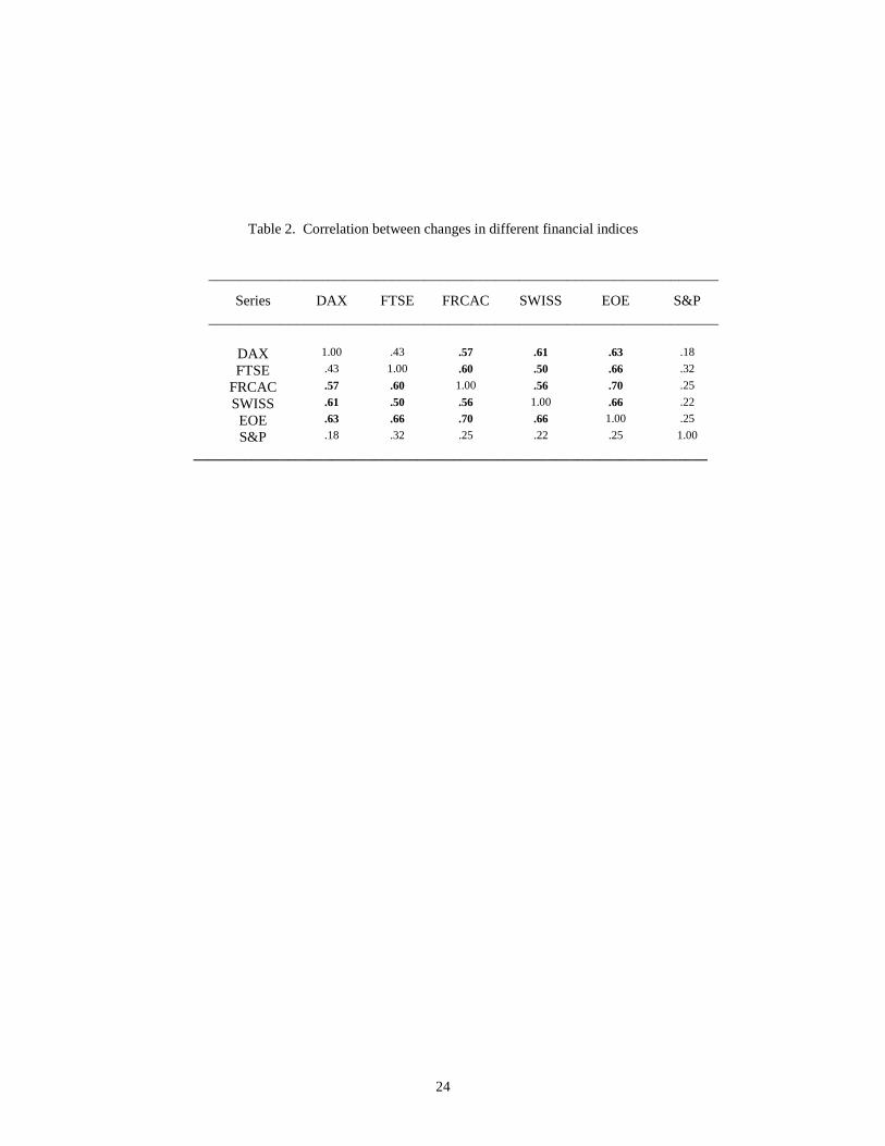
within brackets ( ). Table 2 shows the correlation between returns of different

financial indices. Some stock markets are closely related. This means that market

movements in one country considerably affect the market movement in the

closely related country. All correlation values above .5 have been highlighted.

Since the actual indices show growth with time and they are non stationary, we

perform all of our experiments with the difference series (returns).

10

4. ERROR MEASURES

The selection of appropriate error measures is important in identifying the

differences in the forecasting ability of the PMRS and Neural Networks method.

Fildes [7] notes that several statistical measures should be tried out before

establishing the superiority of forecasting models. The most commonly used

measure in forecasting is the root mean square measure (RMSE). This measure is

very useful in measuring the accuracy of the forecasts but unfortunately it

depends on the scale of the series, Armstrong and Collopy [8]. A more relative

measure is the Mean Absolute Percentage error which shows the error in forecast

relative to the actual value. Armstrong and Collopy [8] note that the RMSE

measure is poor in reliability, fair in construct validity, poor in outlier protection,

good in sensitivity and good in terms of its relationship to decisions. MAPE on

the other hand is fair in reliability, good in construct validity, poor in outlier

protection, good in sensitivity, and fair in terms of relationship to decisions. One

main disadvantage of MAPE is that it puts a heavier penalty on forecasts that

exceed the actual than on those that are less than the actual. Fildes [7] reports that

another important measure is the geometric root mean square error (GRMSE) as it

is well behaved and has a straightforward interpretation. Armstrong and Collopy

[8] also recommend the use of geometric relative absolute error (GMRAE); this

measure has a fair reliability, good construct validity, fair outlier protection, good

sensitivity, and poor relationship to decisions. In general, absolute measurements

are more sensitive and more relevant to decision making than relative measures.

However, they tend to be poorer on outlier protection and reliability. In this paper

11

we select the above four measures for comparing the PMRS and Neural Network

results. We also use the % success in correctly predicting direction of series

change measure which is widely used in the financial markets. We quote the

RMSE, GRMSE, GMRAE measures on a per forecast basis. The formulae for

calculating error measures are shown in Appendix III.

5. EXPERIMENTAL SECTION

In this section we first discuss the various issues involved in developing an

optimal multi-layer perceptron architecture for forecasting. This forecasting

model will be compared with PMRS.

Neural Networks

In the recent past, neural networks have been extensively used for forecasting

stock markets [1-3, 11]. In practice, financial markets depend heavily on the

standard neural network architectures and training algorithms; it will be realistic

to assume that a multi-layer perceptron with backpropagation is a market

standard. In this paper we use the standard MLP architecture for comparison on

forecasting financial indices. The aim is to develop two separate neural networks

for analysis: one for predicting the direction of index change (up or down

movement), and another one for predicting the actuals. We first explain the input

selection process, development of a neural network architecture, and training

procedure.

12

Input/output selection

Gately [2] notes that several outputs may be selected for neural networks. We

could predict the recent index change, the direction of series change, change in

value over the forecast period, whether the trend is up or down, the rate of change,

the quality of making a trade at a given time, volatility or change in volatility. In

our analysis, we develop two separate neural networks: one for predicting the

change in direction (up or down movement) and the other for predicting index

returns. For the first network, the output is coded as a 1 if the series moves up,

and a 0 if it goes down. For the second network, we first predict normalised

returns directly. In this case the network output is a real number between the [0,

1] range.

The selection of inputs depends on what is being forecast (outputs). We use a

linear procedure for determining the inputs to the two networks. We run a linear

regression analysis for predicting the current return using the last ten returns, i.e.

(yt-9, … yt). The relative importance of these inputs in correctly predicting the

output is measured using t-statistic. The five most important variables are selected

for further analysis. Here we make an assumption that the linear input selection is

appropriate for a further non-linear analysis; this is in line with the work done by

Refenes et al. [3]. Hence, for both networks there are the same five inputs. There

is one output which in the first network is a 0 or 1 to predict whether the series

goes up or down, and a real number for the second network to predict the actual

13

changes. The number of hidden nodes are selected using the procedure discussed

below.

Network architecture/hidden nodes

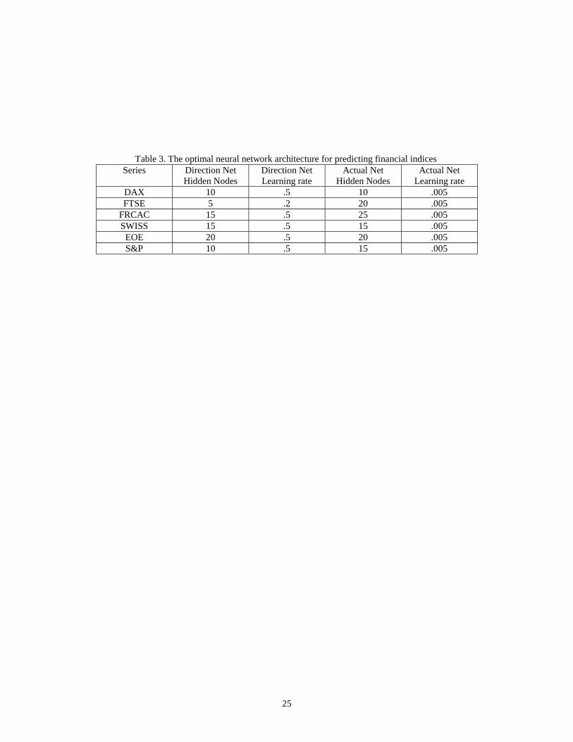
We follow the guidelines set by Weiss and Kulikowski [12]. The aim is to select a

model of minimal complexity which leads to minimal generalisation error. We

increment the number of hidden nodes in a stepwise manner to achieve the

optimal configuration. Table 3 shows the final architectural and training details of

neural networks used for predicting direction and series value of index returns.

Each neural network consists of an input layer, hidden layer and output layer.

Training procedure

The training procedure consists of dividing the data into two parts: estimation

period data and test period data. The estimation period data is used in training. We

use 90% of the total data (total data is 2111 observations in all indices) in the

estimation period and the remaining 10% in the test set. The training/test

procedure is performed using the Stuttgart Neural Network Simulator using the

standard backpropagation algorithm.

6. RESULTS

The first result comes from PMRS predicting the direction of series change;

positive or negative relative to the current position. This is one of the most

important measures in financial markets. The results for the different financial

14

indices are shown in Table 4. For all indices, PMRS and Neural Network models

are able to predict nearly three out of four times the correct direction of move. In

Table 4 shows that the PMRS algorithm is very good at predicting the direction of

the series change. This confirms that the match between the current market

situation and the historical market situation is a crucial link for making accurate

forecasts. The PMRS and NN performances are equally good on FRCAC and

S&P index. The neural network is better on DAX and FTSE index whereas PMRS

is better on SWISS and EOE. Traders in the financial markets are very much

interested in forecasting the direction of index change. At a given time, the value

of the index is known. The knowledge whether the financial index will be higher

or lower the next day is important for the trading buy-sell-hold strategy. If the

index value will be lower the next day, it may be useful to sell stocks, if it will be

higher then it is better to hold on to your stocks and buy some now. A number of

international companies that deal with more than one currency for business are

also heavily dependent on the market changes. The ability to correctly forecast the

direction of index change translates easily into the exchange rates of currencies

and companies can save monies with large transactions through accurate

predictions, Levich [13]. We next compare the RMSE, MAPE, GRMSE and

GMRAE error measures of the two methods in Table 5.

In Table 5, the PMRS algorithm and Neural Networks perform significantly well.

We compare the best PMRS and neural network models. The arithmetic Root

Mean Square Error (RMSE), Geometric Root Mean Square Error, and Mean

15

Absolute Percentage error is lower for neural networks. Neural networks also

have a slight edge over PMRS when compared to a random walk model shown by

the GMRAE measure. The error measure GMRAE is important in measuring how

well both models perform compared to the random walk model. The best method

on this measure will generate a value of 0, the worst value will be ∞, and when

the proposed method performs as good as the random walk model, then GMRAE

should be equal to 1. Hence, the lower the value on this measure, relative to 1, the

better the proposed method is compared to random walk. Since RAE is a ratio, in

order to calculate how many times better than random walk, we can take an

inverse of the value generated on this measure. For example, on DAX prediction,

the difference between a random walk output and the actual series value is 90

times more than the difference between PMRS prediction and actual series value,

and 125 times more for neural networks. The results are similar for other indices.

The key finding is that PMRS performs very efficiently and is quite close to

neural network performance on several measures. These results coupled with

Table 4 show that the PMRS algorithm is both accurate in forecasting the

direction and magnitude of change. Without a doubt, PMRS approach offers the

promise of better performance than neural networks with further modification.

An important step towards establishing PMRS as a good forecasting model is to

show that the errors in prediction are not biased (low auto-correlation between

error at different lags). Table 6 shows the auto-correlation between the PMRS

16

residuals at different lags. Fortunately, the auto-correlations are low proving that

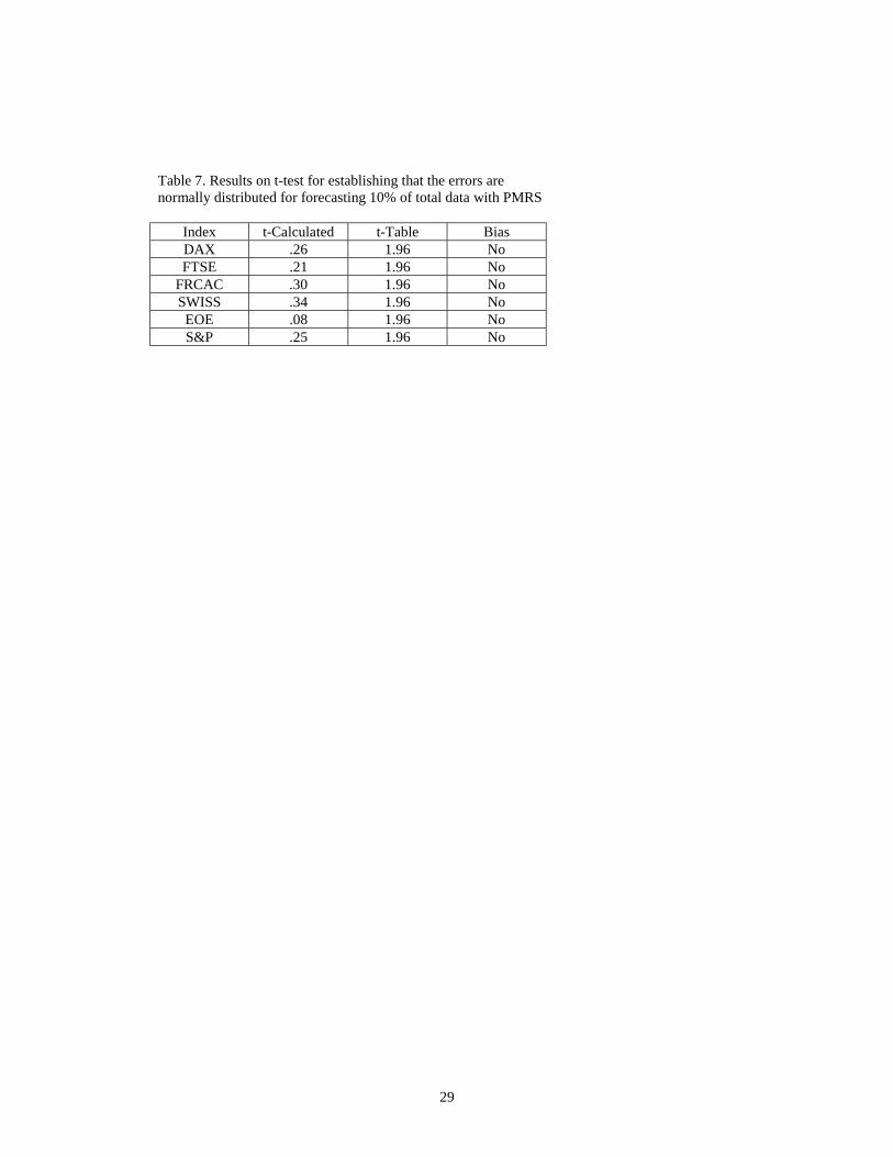
the forecasts are not biased in either direction. We also use a t-test to confirm

whether the mean error is statistically significantly different from zero,

Delurgio[9]. The simple test is:

Null hypothesis: ê = 0; if this hypothesis is proven wrong, then accept

Alternative hypothesis: ê < 0 or ê > 0

A calculated t value is compared to the t-value from the t-table. If the calculated

value is less than or equal to the table value then we accept the null hypothesis,

and otherwise we reject it. The t value from the table for 95% confidence for

n=210 samples (10% of total samples are predicted) is equal to 1.96. The t value

is calculated by:

t-calculated = ê /(Se/√n)

where ê is the mean error, Se is standard deviation of errors about the mean ê and

n is the total number of samples. Table 7 shows the results for all indices. In each

case, we accept the null hypothesis leading us to conclude that there is no bias and

95 percent of the errors lie within 1.96 standard errors of the mean value of zero.

The PMRS algorithm can be improved on these measures by following these

guidelines:

17

• The PMRS algorithm could be optimised for the weights wi as shown in

Figure 1. In this paper, we have used all wi = 1.

• The PMRS algorithm could be capped for a maximum and a minimum

forecast avoiding wild estimates.

• The PMRS algorithm can select more than one nearest neighbour segments

when matching and take an average of forecasts based on them. This

technique may also be tried using extrapolation.

• One important advantage of PMRS is their real-time functioning. On a

Pentium 200 MHz processors, it takes less than 1 second per forecast.

We next take one month August 1996 data of the different financial indices

and plot both PMRS and NN predictions against the actuals. We only plot one

month’s data since larger plots do not exhibit in sufficient detail the differences

between the actual and predicted values. Figures 2 to 7 in Appendix I show the

plots of the different time-series predictions. As it can be seen, the PMRS

forecasts are accurate in following the trend of the time series and the daily

changes. This argument is further supported by the scatter plots shown in

Appendix II. The plots show strong positive correlation between actual series

values and PMRS predictions.

7. CONCLUSION

In this paper we have shown that a pattern recognition algorithm for forecasting is

an alternative solution to using statistical methods that have limitations in non-

18

linear domains, or neural networks that have long training times and require

substantial experience in their prior use. The PMRS performance was found to be

in close competition with neural networks; it is expected that further research on

these predictors will yield superior results in the future. The PMRS tool is

attractive for several reasons: i) pattern matching tasks approximate local

neighbourhoods; ii) such tools require lesser number of parameters that need

optimisation compared to sophisticated recurrent and backpropagation networks;

and iii) PMRS works in real-time because of its non-iterative nature unlike neural

networks, and are particularly suited in stock markets for predicting tick-type

data. A short memory system uses inputs (yt-h, … yt) for predicting yt and it has a

memory equal to h. However, for a long memory system such as PMRS, the

memory h for different test patterns is dynamic and is determined by the matching

process. One important advantage of PMRS is that the historical memory

triggered teaches us something about the time-series (trading behaviour). The

distance between the current time, and the historical time when memory was

triggered, i.e. value of h, showing the closest match can be statistically studied.

Table 8 shows the memory characteristics of PMRS showing an average memory

of more than 1000 days. It is interesting to note that the average memory across

different markets is very similar and quite large. These results are in agreement

with Peters [4] which confirm that financial markets have long memories of

approximately four years. The minimum and maximum values in the table show

how extreme these memories can become. Finally, the standard deviation shows

how varied these memories are across different test patterns; the standard

19

deviations are very large which emphasises that a dynamic rather than fixed

model for prediction is a more natural way of forecasting financial series. Some of

the work on using pattern recognition techniques for stock market forecasting has

been recently implemented in the Norwegian stock market with encouraging

results [14]. We expect that PMRS technology will be further developed and fine-

tuned for practical trials.

20

REFERENCES

[1] M. E. Azoff, Neural Network Time Series Forecasting of Financial

Markets, John Wiley, 1994.

[2] E. Gately, Neural Networks for Financial Forecasting, John Wiley, 1996.

[3] A. N. Refenes, N. Burgess and Y. Bentz, “Neural networks in financial

engineering: A study in methodology,” IEEE Transactions on Neural

Networks, vol. 8, no. 6, pp. 1222-1267, 1997.

[4] E. Peters, Fractal Market Hypothesis: Applying Chaos Theory to

Investment and Economics, John Wiley, 1994.

[5] J. D. Farmer, and J. J. Sidorowich, Predicting chaotic dynamics, in

Dynamic patterns in complex systems, J. A. S. Kelso, A. J. Mandell and

M. F. Shlesinger (Eds.), pp. 265-292, Singapore: World Scientific, 1988.

[6] B. S. Motnikar, T. Pisanski and D. Cepar “Time-series forecasting by

pattern imitation”, OR Spektrum, 18(1), pp. 43-49, 1996.

[7] R. Fildes, “The evaluation of extrapolative forecasting methods”,

International Journal of Forecasting, vol. 8, pp. 81-98, 1992.

[8] J. S. Armstrong, J. S. and F. Collopy, “Error measures for generalising

about forecasting methods: Empirical comparisons”, International

Journal of Forecasting, vol. 8, pp. 69-80, 1992.

[9] S. Delurgio, Forecasting: Principles and applications, McGraw-Hill,

1988.

21

[10] S. Makridakis, A. Andersen, R. Carbone, R. Fildes, M. Hibon, R.

Lewandowski, J. Newton, E. Parzen and R. Winkler, The forecasting

accuracy of major time-series methods, Chichester: John Wiley, 1984.

[11] J. Kingdon, Intelligent Systems for Financial Engineering, Springer, 1997.

[12] S. M. Weiss, and C. A. Kulikowski, Computer systems that learn, Morgan

Kaufmann, San Mateo, CA, 1991.

[13] Levich, R. M., International Financial Markets: Prices and Policies,

McGraw-Hill, 1987.

[14] Linlokken, G., “Syntactical pattern recognition in financial time-series,”

Proceedings of the Norwegian Image Processing and Pattern Recognition

Society Conference, Oslo, 1996.

Figure 1. Flowchart for the PMRS forecasting algorithm

k = k+1

= 0 (predict low)

Yes

Startk=2

Find closestMini

Predict lowÿn+1= yn - β*δj+1, where

kβ = 1/k ∑ δn-i/δj-i

i=1

Choose a pattern of size k

ρ’ = (bn-2, bn-1).

= 1 (predict high)

historical match of ρ’ which is ρ’’ = (bj-1, bj) bymising offset ∇ , j is the marker position

k∇ = ∑ wi(δn-i - δj-i) i=1

bj ?

Predict highÿn+1= yn + β*δj+1, where

kβ = 1/k ∑ δn-i/δj-I

i=1

Calculate MSE, MAPE, GRMSE, GMRAE, and Directionerror where(Direction error) = error when yn+1 - yn > 0 and ÿn+1 - yn ≤ 0

and error when yn+1 - yn ≤ 0 and ÿn+1 - yn > 0

22

NoChoose PMRS model with

smallest pattern size k whichyields minimal error

measurements

end

k < kmax

23

Table 1. Financial series statistics

_________________________________________________________________________

Series Min Max Mean SD Size Autocorrelationr(yt, yt-1)

___________________________________________________________________________

DAX 1152 2583 1798 347 2111 .99 (-.50)

FTSE 1730 3857 2718 550 2111 .99 (-.48)

FRCAC 1276 2355 1862 201 2111 .99 (-.47)

SWISS 1287 3810 2165 635 2111 .99 (-.46)

EOE 729 1458 1030 187 2111 .99 (-.47)

S&P 257 678 422 100 2111 .99 (-.50)

__________________________________________________________________________________

24

Table 2. Correlation between changes in different financial indices

________________________________________________________________

Series DAX FTSE FRCAC SWISS EOE S&P________________________________________________________________

DAX 1.00 .43 .57 .61 .63 .18

FTSE .43 1.00 .60 .50 .66 .32

FRCAC .57 .60 1.00 .56 .70 .25

SWISS .61 .50 .56 1.00 .66 .22

EOE .63 .66 .70 .66 1.00 .25

S&P .18 .32 .25 .22 .25 1.00

_______________________________________________________________________

25

Table 3. The optimal neural network architecture for predicting financial indicesSeries Direction Net

Hidden NodesDirection NetLearning rate

Actual NetHidden Nodes

Actual NetLearning rate

DAX 10 .5 10 .005FTSE 5 .2 20 .005

FRCAC 15 .5 25 .005SWISS 15 .5 15 .005

EOE 20 .5 20 .005S&P 10 .5 15 .005

26

Table 4. The direction success rate % for the predicting differentfinancial indices using PMRS with varying segment size k andNeural Networks (forecasting 10% of total data)

________________________________________________________

Index Optimal k PMRS NN % sizepredicted

________________________________________________________

DAX 5 73 77 10

FTSE 5 71 75 10

FRCAC 3 72 72 10

SWISS 3 72 67 10

EOE 3 75 74 10

S&P 3 76 76 10

______________________________________________________________

27

Table 5. The best performances of PMRS and Neural Networksforecasting 10% of total data

_______________________________________________________

SeriesMethod

SegmentsK

RMSE MAPE GRMSE GMRAE

_______________________________________________________

DAXPMRS

NN5 3.1

2.01.51.4

1.81.1

.011

.008FTSE

PMRSNN

5 3.42.6

1.11.3

1.81.4

.010

.008FRCAC

PMRSNN

3 2.61.4

1.51.3

1.61.0

.008

.004SWISS

PMRSNN

2 4.82.3

1.51.2

2.51.4

.011

.003EOE

PMRSNN

3 1.31.0

1.1 1.3

0.70.6

.008

.007S&P

PMRSNN

3 0.60.4

1.11.1

0.30.2

.008

.004_____________________________________________________________

28

Table 6. Auto-correlation r between residuals at time lags 1 to 5 forforecasting 10% of total data using PMRS

Series r(et, et-1) r(et, et-2) r(et, et-3) r(et, et-4) r(et, et-4)

DAX -.65 .17 -.08 .14 -.13FTSE -.68 .25 -.14 .16 -.14

FRCAC -.65 .17 -.04 .07 -.06SWISS -.57 .27 -.21 .19 -.10EOE -.63 .17 -.11 .19 -.17S&P -.50 .12 -.09 .08 -.08

29

Table 7. Results on t-test for establishing that the errors arenormally distributed for forecasting 10% of total data with PMRS

Index t-Calculated t-Table BiasDAX .26 1.96 NoFTSE .21 1.96 No

FRCAC .30 1.96 NoSWISS .34 1.96 NoEOE .08 1.96 NoS&P .25 1.96 No

30

Table 8. Memory statistics for the PMRS algorithm on forecasting 10% of financial index data

Series Min Mean Max Std. Dev.DAX 24 1007 2040 583FTSE 89 1117 2029 508

FRCAC 54 1019 2062 553SWISS 47 884 1998 523

EOE 51 789 2000 458S&P 35 1126 2051 505

31

Appendix I

Figure 2. DAX forecasts and actual index value for August 1996

Figure 3. FTSE forecasts and actual index value for August 1996

2300

2400

2500

2600

2700

1 4 7 10 13 16 19 22 25 28

time

FI

actual

N-net

PMRS

3500

3600

3700

3800

3900

1 4 7 10 13 16 19 22 25 28

time

FI

actual

N-net

PMRS

32

Figure 4. FRCAC forecasts and actual index value for August 1996

Figure 5. SWISS forecasts and actual index value for August 1996

1800

1900

2000

2100

2200

1 4 7 10 13 16 19 22 25 28

time

FI

actual

N-net

PMRS

3300

3400

3500

3600

3700

3800

3900

1 4 7 10 13 16 19 22 25 28

time

FI

actual

N-net

PMRS

33

Figure 6. EOE forecasts and actual index value for August 1996

Figure 7. S&P forecasts and actual index value for August 1996

1300

1400

1500

1 4 7 10 13 16 19 22 25 28

time

FIactual

N-net

PMRS

600

620

640

660

680

700

1 3 5 7 9 11 13 15 17 19 21 23 25 27 29

time

FIactual

N-net

PMRS

34

Appendix II. Scatter plots for PMRS forecasts

FRCAC scatter plot

1600

1700

1800

1900

2000

2100

2200

2300

1600 1700 1800 1900 2000 2100 2200

Actuals

PM

RS

fo

reca

st

DAX scatter plot

2000

2100

2200

2300

2400

2500

2600

2700

2000 2100 2200 2300 2400 2500 2600 2700

Actuals

PM

RS

fo

reca

st

EOE scatter plot

1200

1250

1300

1350

1400

1450

1500

1200 1250 1300 1350 1400 1450 1500

Actuals

PM

RS

fo

reca

st

FTSE scatter plot

3450

3550

3650

3750

3850

3950

3450 3500 3550 3600 3650 3700 3750 3800 3850 3900

Actuals

PM

RS

fo

reca

st

S&P scatter plot

560

580

600

620

640

660

680

700

560 580 600 620 640 660 680 700

Actuals

PM

RS

fo

reca

st

Swiss scatter plot

3000

3200

3400

3600

3800

4000

3000 3200 3400 3600 3800 4000

Actuals

PM

RS

fo

reca

st

35

APPENDIX III. Error measures

m is the forecasting method

rw is the random walk method

s is the series being forecast

Fm,s is the forecast from method m for series s

Am,s is the actual value for series s

Root mean square error per forecast

Mean Absolute Percentage Error

Geometric Root Mean Square Error per forrecast

Relative Absolute Error

Geometric Relative Absolute Error per forecast

=RMSEm ))((/1 2/12

1,∑ −

=

N

nssm AFN

=MAPEm AAFN s

N

nssm /|))(|(/100

1,∑ −

=

=GRMSE m ))((/1 2

1

1

2, N

N

nssm AFN ∏ −

=

=RAEm||

||

,

,

AF

AF

ssrw

ssm

−−

=GMRAEm ))((/11

1N

m

N

nRAEN ∏

=