long-period ground motions from past and virtual

Ⓔ

Long-Period Ground Motions from Past and Virtual Megathrust

Earthquakes along the Nankai Trough, Japan

by Loïc Viens* and Marine A. Denolle

Abstract Long-period ground motions from large (Mw ≥ 7:0) subduction-zoneearthquakes are a real threat for large-scale human-made structures. The Nankaisubduction zone, Japan, is expected to host a major megathrust earthquake in the nearfuture and has therefore been instrumented with offshore and onshore permanentseismic networks. We use the ambient seismic field continuously recorded at thesestations to simulate the long-period (4–10 s) ground motions from past and futurepotential offshore earthquakes. First, we compute impulse response functions (IRFs)between an ocean-bottom seismometer of the Dense Oceanfloor Network System forEarthquakes and Tsunamis (DONET) network, which is located offshore on the accre-tionary wedge, and 60 onshore Hi-net stations using seismic interferometry by decon-volution. As this technique only preserves the relative amplitude information of theIRFs, we use a moderate Mw 5.5 event to calibrate the amplitudes to absolute levels.After calibration, the IRFs are used together with a uniform stress-drop source modelto simulate the long-period ground motions of the 2004Mw 7.2 intraplate earthquake.For both events, the residuals of the 5% damped spectral acceleration (SA) computedfrom the horizontal and vertical components of the observed and simulated waveformsexhibit almost no bias and acceptable uncertainties. We also compare the observed SAvalues of the Mw 7.2 event to those from the subduction-zone BC Hydro ground-motion model (GMM) and find that our simulations perform better than the model.Finally, we simulate the long-period ground motions of a hypothetical Mw 8.0 sub-duction earthquake that could occur along the Nankai trough. For this event, our sim-ulations generally exhibit stronger long-period ground motions than those predictedby the BC Hydro GMM. This study suggests that the ambient seismic field recordedby the ever-increasing number of ocean-bottom seismometers can be used to simulatethe long-period ground motions from large megathrust earthquakes.

Supplemental Content: Text and figures detailing the raw impulse responsefunctions (IRFs) from the KMD14 virtual source, the correction applied to the IRFamplitudes to account for the nonuniform source of the ambient seismic field, andthe raw IRFs and noise levels at the KMC10 and KMC11 virtual sources, the effectof the surface-wave radiation pattern at periods longer than 10 s for the two earthquakes,the determination of the source parameters for the simulation of theMw 7.2 earthquake,and the attenuation of spectral acceleration values with distance for the Mw 7.2 event.

Introduction

Large (Mw ≥ 7:0) subduction-zone earthquakes can gen-erate strong and long-duration low-frequency seismic waves atgreat distances from the source. Such ground motions are gen-erally the result of an efficient propagation of seismic wavesthrough elastic structures such as accretionary wedges or

sedimentary basins (Koketsu et al., 2008). In urban environ-ments, long-period seismic waves are of particular concerndue to the increasing number of large-scale structures suchas tall buildings and long-span bridges. One of theworst exam-ples of damage caused by long-period ground motionsoccurred during the 1985 Mw 8.0 Michoacán earthquake inMexico City, where hundreds of buildings were destroyedor badly damaged due to sedimentary basin amplification

*Now at Disaster Prevention Research Institute, Kyoto University,Gokasho, Uji, Kyoto 611-0011, Japan.

BSSA Early Edition / 1

Bulletin of the Seismological Society of America, Vol. XX, No. XX, pp. –, – 2019, doi: 10.1785/0120180320

Downloaded from https://pubs.geoscienceworld.org/ssa/bssa/article-pdf/doi/10.1785/0120180320/4753601/bssa-2018320.1.pdfby Harvard University useron 22 July 2019

(Anderson et al., 1986;Beck andHall, 1986).Another exampleis the serious damage to large oil-storage tanks in the city ofTomakomai, Japan, caused by the long-period ground motionsfrom the 2003Mw 8.3 Tokachi-Oki earthquake,which occurredmore than 250 km away offshore (Koketsu et al., 2005).

To assess the seismic hazard related to short- and long-period ground motions, ground-motion models (GMMs),also called ground-motion prediction equations, have beendeveloped specifically for subduction-zone earthquakes(e.g., Crouse et al., 1988; Youngs et al., 1997; Atkinsonand Boore, 2003, 2008; Zhao et al., 2006; BC Hydro,2012; Abrahamson et al., 2016). These empirical relationsrelate the source, path, and site parameters to the ground-motion levels from intraplate and interplate earthquakes insubduction zones and generally capture well the character-istics of the high-frequency ground motions, including non-linear effects. For a specific subduction zone, however, thecrustal structure (e.g., accretionary wedge and sedimentarybasin effects) may have a strong influence on the long-periodground motions, which might not be adequately representedby GMMs. This is in part due to the fact that GMMs aregenerally developed using strong ground motion recordsfrom different regions and may not contain the path effectrelevant to a specific subduction zone. To better understandthe long-period wave propagation effects from offshore sub-duction events, physics-based simulations using simple butrealistic velocity models of subduction zones have been per-formed (e.g., Furumura et al., 2008; Yoshimura et al., 2008;Guo et al., 2016). These simulations indicate that accretion-ary wedges may attenuate long-period ground motions butextend their duration through the development of complexcoda waves. Although these conclusions agree relatively wellwith observed earthquake waveforms, simulations are stilllimited by our imperfect knowledge of the elastic and ane-lastic structure of the Earth, especially near the trench.

In the last decade, seismic interferometry has becomevery popular in seismology. Under certain conditions, thecross correlation of ambient seismic field records at two seis-mometers is proportional to the elastodynamic response of theEarth, or impulse response function (IRF), between the twostations (Shapiro and Campillo, 2004; Sabra et al., 2005).Therefore, the phase information of the IRF closely capturesthat of the true Green’s function, in particular for surfacewaves, and has been widely used to image the Earth’s struc-ture (e.g., Shapiro et al., 2005; Lin et al., 2008). On the otherhand, the amplitude information is, in theory, less reliable dueto the data processing and the nonideal location of the ambientseismic field sources (Tsai, 2011; Weaver, 2011; Stehly andBoué, 2017). Nevertheless, several empirical and numericalstudies have shown promising results in retrieving reliableattenuation measurement (Lawrence and Prieto, 2011;Lawrence et al., 2013) and in simulating earthquake groundmotions (e.g., Prieto and Beroza, 2008; Viens et al., 2017).

Seismic interferometry with deconvolution has beenused to successfully simulate the long-period ground shakingfrom earthquakes in different geological and tectonic

contexts. The long-period seismic waves from moderateMw 4–5 onshore earthquakes, in which the point-sourceapproximation is valid at long periods, have been simulatedin the United States (Prieto and Beroza, 2008; Denolle et al.,2013; Sheng et al., 2017) and Japan (Viens et al., 2014).Kwak et al. (2017) also applied this technique to simulatethe long-period waves generated by a mine collapse event(Mw 4.2) in South Korea. Large past and hypothetical futurecrustal earthquakes, in which finite faults need to be takeninto account, have also been simulated (Denolle et al., 2014;Viens, Miyake, et al., 2016; Denolle et al., 2018). Finally, theseismic interferometry technique has been shown to success-fully recover 3D wave propagation effects in sedimentarybasins, where the complex seismic wave propagation andamplification caused by the velocity structure is captured bythe IRFs (Denolle et al., 2014; Boué et al., 2016; Viens,Koketsu, et al., 2016). The simulation of long-period groundmotions from subduction earthquakes with ambient seismicfield IRFs, however, has only been the focus of one study(Viens et al., 2015), due to the lack of offshore seismic net-works. The deployment of ocean-bottom seismometers insubduction zones worldwide and the recent availability andaccessibility of their data offer the opportunity to investigatethe potential of seismic interferometry to simulate the long-period ground motions from large and megathrust earthquakes.

In southwest Japan, the subduction of the Philippine Seaplate beneath the Eurasian plate along the Nankai trough iswell known to hostMw 8 and greater megathrust earthquakesabout every 100–200 yr (Ando, 1975). To monitor the real-time seismic activity in this region, the Dense OceanfloorNetwork System for Earthquakes and Tsunamis (DONET)was deployed by the Japan Agency for Marine-EarthScience and Technology (Kaneda et al., 2015; Kawaguchiet al., 2015). The DONET 1 network has been operationalsince 2011 and is composed of 20 stations with both broad-band and strong-motion three-component sensors (Fig. 1).The most recent large events along the Nankai trough occurredin 2004 during the Off the Kii peninsula earthquake sequence,with an Mw 7.2 intraplate event that was followed 5 hr laterby an Mw 7.5 intraplate earthquake. Although the DONET 1network was not installed at the time of the earthquakes, theground motions from these events were well recorded onshoreby the different networks of the National Research Institute forEarth Science and Disaster Resilience (NIED; e.g., F-net,Hi-net, KiK-net, and K-NET; Okada et al., 2004; Obara et al.,2005). The recorded waveforms exhibit large long-periodamplifications in the Osaka, Nagoya, and Kanto sedimentarybasins (Miyake and Koketsu, 2005).

In this study, we focus on the simulation of long-period(4–10 s) ground motions from past and future potential off-shore earthquakes along the Nankai trough using the ambientseismic field. First, we introduce the data and our method-ology as well as the metrics that are used for quality assess-ment. We also briefly introduce the subduction-zone BCHydro GMM developed by Abrahamson et al. (2016) thatis used to cross-validate our results. We then simulate two

2 L. Viens and M. A. Denolle

BSSA Early Edition


earthquakes that occurred in 2004, a moderate Mw 5.5 eventand theMw 7.2 intraplate earthquake. We compare the simu-lated and observed long-period ground motions for these twoevents and cross-validate their spectral acceleration (SA) val-ues with those from the GMM. Finally, we simulate a poten-tial Mw 8.0 megathrust event that could occur along theNankai trough, and compare the SA values of the predictedwaveforms with those from the GMM.

Data and Methods

IRF Computation

We use four months of continuous data recorded from 1June to 30 September 2015 by one DONET station (e.g.,KMD14 station) and 60 Hi-net stations located in the surround-ing area (Fig. 1). The study by Takagi et al. (2018) recentlyshowed that the Pacific Ocean is the main source of surface

waves during the summer season and thatthe Japan Sea generates most surface wavesduring winter months in the 4–8 s periodband, which is similar to our focus on the4–10 s period range. By selecting the datarecorded during summer months, the distri-bution of ambient-noise sources favors thecoherence of the signal from offshore toonshore paths near the Nankai trough, thusenhancing the quality of the IRFs.

The broadband seismometers of theDONET 1 network record continuous datawith a 100 Hz sampling rate, and mostsensors are buried in shallow 1-meter-deepboreholes. The Hi-net stations also recordat 100 Hz and are located in boreholes withdepths ranging between 100 and 3000 m.Although Hi-net seismometers are high-sensitivity sensors with a cutoff periodof 1 s, reliable long-period (≥1 s) seismicwaves can also be retrieved after correctingfor the instrumental response thanks to thewide dynamic range of the recording system(Obara et al., 2005). We correct the DONETand Hi-net data for their instrumentalresponses and rotate their horizontal compo-nents to the true north–south and east–westdirections using the orientations determinedby Nakano et al. (2012) and Shiomi (2013).

For each seismic station, we down-sample the velocity data recorded by thethree-component sensors to 10 Hz anddivide them into 1-hour-long time series.To reduce the unwanted effects of transientsignals from earthquakes, we discard thetime windows with peaks greater than 10times the standard deviation of the win-dow. For each station pair, we compute

the IRFs between the vertical, north, and east componentsusing the deconvolution technique. This computation is per-formed in the frequency domain with a smoothing operatorapplied to the denominator spectrum using a moving averageover 20 points. Additional details about the deconvolutionmethod applied in this study can be found in Viens et al.(2017). The 1 hr IRFs are finally stacked together to improvethe signal-to-noise ratio (SNR), time differentiated once toretrieve the proportionality between cross-correlation func-tion and Green’s function (Snieder, 2004; Roux et al.,2005; Prieto et al., 2011), and band-pass filtered between4 and 10 s using a four-pole and two-pass Butterworth filter.We rotate the nine-component Green’s tensor from the east–north–vertical (ENZ) coordinate system to the radial–trans-verse–vertical (RTZ) system for each station pair. By rotatingthe IRFs, we suppose that Rayleigh waves are retrieved on theZ–Z and R–R components and that Love waves are retrievedon the T–T component.

Figure 1. Topographic map of the Kii peninsula region and the Nankai subductionzone including the Hi-net and Dense Oceanfloor Network System for Earthquakes andTsunamis (DONET 1) stations (triangles). The focal mechanisms of the 2004 Mw 5.5and 7.2 earthquakes are shown together with their respective epicenters (stars). The con-tour of the fault plane of the 2004Mw 7.2 event projected at the surface is shown by therectangle. The KMD14 station is the virtual source station used to compute offshore–onshore impulse response functions (IRFs) and its location is shown by the large tri-angle. KMC10 and KMC11 stations are the closest stations from the epicenter of theMw 5.5 event. The names of eight Hi-net stations used in this study are also indicated.(Inset) The Japan Islands and the rectangle is the region of interest. The color version ofthis figure is available only in the electronic edition.

Long-Period Ground Motions from Past and Virtual Megathrust Earthquakes along the Nankai Trough 3

BSSA Early Edition


We show the IRFs for the T–T, R–R, and Z–Z componentscomputed using the data recorded between June and September2015 in Figure 2, and the six other components of the Green’stensor in Ⓔ Figure S1 (available in the supplemental contentto this article). Propagating seismic waves can be observed onboth anticausal (negative) and causal (positive) sides of theIRFs. As the amplitude of the causal part of the IRF is likelyto better capture site amplification and attenuation effects thanthe anticausal part (Bowden et al., 2015; Liu et al., 2016), weonly consider the causal part of the IRFs in this study. To char-acterize the potential bias of the IRF amplitudes caused by var-iations of ambient seismic field sources, we compute the SNRfor the T–T, R–R, and Z–Z IRFs. The SNR is defined as thepeak amplitude of the causal IRFs band-pass filtered between 4and 10 s over the root mean square level of the 25 s preceding avelocity of 3:0 km=s for each station. The SNR values plottedagainst the azimuth from the virtual source (e.g., KMD14 sta-tion) are shown in Ⓔ Figure S2. Although there is almost novariation of the SNR with azimuth for the Z–Z component,there is some variation in the SNR of the R–R and T–T com-ponents. To reduce the amplitude biases, we first correct theIRF amplitudes for their surface-wave theoretical geometricalspreading (multiplication by

��dv−r

p, in which dv−r is the virtual

source–receiver distance) and show the peak values as a func-tion of the azimuth from the virtual source inⒺ Figure S3. Wethen model the small azimuthal variations by fitting the peakamplitudes of the IRFs corrected for the surface-wave geo-metrical spreading with a third degree polynomial. We finallycorrect the IRF amplitudes by multiplying the waveforms bythe ratio of the polynomial function value at the correspondingazimuths over the mean amplitude of the data.

Earthquake Data

For the Mw 5.5 and Mw 7.2 earthquakes considered inthe following sections, earthquake records at Hi-net stations

are first corrected for their instrumental responses to retrievethe velocity ground motion and the horizontal componentsare rotated to the true north–south and east–west directionsusing the orientations determined by Shiomi (2013). Foreach earthquake, the horizontal components are then rotatedto R and T directions from the earthquake epicenter. Finally,the velocity data from the three components are down-sampled to 10 Hz and band-pass filtered between 4 and 10 susing a four-pole and two-pass Butterworth filter.

Source Models

Moderate Earthquake Simulation. We first focus on thesimulation of an Mw 5.5 earthquake, which occurred on10 September 2004 at 11:05 a.m. (Japan Standard Time[JST]) at a depth of ˜5 km (NIED centroid moment tensorsolution). As mentioned in the IRF Computation section,the IRFs are computed between the KMD14 station, whichis located ˜26 km away from the epicenter in a shallow1-meter-deep borehole, and onshore Hi-net stations. Thisallows us to retrieve better-quality IRFs than with theKMC10 and KMC11 stations, which are located closer to theepicenter but directly on the seafloor (Fig. 2 andⒺ Fig. S4).As mentioned in several studies (e.g., Stutzmann et al., 2001;Crawford et al., 2006), seismometers located directly on theseafloor are subject to additional noise sources, thus leadingto a higher noise level, especially for the horizontal compo-nents (Ⓔ Fig. S5). Although some techniques have beendeveloped to reduce the noise levels (Crawford and Webb,2000), we leave this task to future work. To correct for thedifference in location between the earthquake epicenter andthe KMD14 virtual source, we simply time shift the IRFsconsidering a constant surface-wave velocity of 3:2 km=s,assuming that the surface-wave dispersion is weak in thenarrow frequency band of interest. This value corresponds to˜90% of the average S-wave velocity in the upper 15 km of

Figure 2. Causal (positive) and anticausal (negative) parts of the IRFs for the T–T, R–R, and Z–Z components as a function of thedistance to the virtual source (KMD14). All waveforms are band-pass filtered between 4 and 10 s and dashed lines represent the3:0 km=s moveout. The color version of this figure is available only in the electronic edition.


BSSA Early Edition


the crust following the Japan Integrated Velocity StructureModel (JIVSM, Koketsu et al., 2009, 2012). We also correctthe amplitude of the IRFs to account for the difference insurface-wave geometrical spreading between the virtualsource–receiver (dv−r) and the epicenter–receiver (de−r)distances (e.g., multiplication by

��dv−r

p=

��de−r

p). Finally,

we taper the IRFs to remove the spurious and nonphysicalsignals that appear to travel faster than 6 km=s and maycontaminate the IRFs (e.g., Shapiro et al., 2006; Zeng andNi, 2010).

To simulate the velocity waveforms of a moderate earth-quake, the T–T, R–R, and Z–Z IRFs are convolved with asource time function. For theMw 5.5 event, which is approxi-mated as a point source at the periods of interest, we use atriangle moment-rate function as the source time function.The duration of this function (Tr) is based on the moment-duration relation from Somerville et al. (1999) that is definedas Tr � 2:03 × 10−9 × �m0=107��1=3�, in which m0 is theseismic moment of theMw 5.5 event in N · m. For this event,we obtain a source time function duration Tr of 0.26 s, whichis rounded to 0.3 s given our 10 Hz sampling rate. The ampli-tude of the source time function is set so that its integral overits duration is equal to the seismic moment of the Mw 5.5event (e.g., 2:22 × 1017 N · m).

After convolving the IRFs with the source time function,the simulated velocity waveforms need to be calibrated withthe earthquake velocity seismograms as only the relative,rather than absolute, IRF amplitude is retrieved from theambient seismic field. A calibration factor for each compo-nent of the IRF (e.g., Z–Z, R–R, and T–T) but common to allstations is calculated as follows. First, the absolute value ofthe Fourier transform amplitude of both the recorded andsimulated velocity waveforms for all the stations is com-puted. Then, the absolute values are averaged over the 4–10 speriod range and over the number of stations for both therecorded and simulated waveforms. Finally, the calibrationfactor is computed as the ratio of the observed over simulatedvalues, similarly as in Viens et al. (2014). For each compo-nent, the simulated velocity waveforms are multiplied bytheir respective calibration factor. The calibration factorscomputed using the Mw 5.5 event for each component areused to calibrate the IRFs for the computation of large earth-quakes in the following sections.

Radiation pattern effects matter when simulating groundmotions at a wide range of source–receiver paths, in particu-lar when the paths sample the nodal planes of the radiationpattern. Denolle et al. (2013) proposed to correct the surfaceimpulse responses to the displacements that are radiated froma buried double-couple point source for moderate and shal-low Californian earthquakes. For the Mw 5.5 earthquake ofinterest, the observed ground motions do not exhibit clearazimuthal variations that would be indicative of radiationpattern effects in the 4–10 s period range. To demonstratethis feature, we first correct the simulated and observedwaveforms for the surface-wave geometrical spreading bymultiplying them by

��de−r

p. For the three components, we

show the simulated and observed long-period peak groundvelocity (PGV) values after surface-wave geometrical spread-ing correction as a function of the azimuth from the epicenterin Figure 3a and 3b, respectively. These values are com-puted for waves traveling slower than 3:0 km=s to reducethe effect of body waves and primarily focus on surface waves.We also compute the theoretical surface-wave (both Love andRayleigh) amplitudes expected given the radiation pattern ofthe NIED moment tensor solution and the JIVSM profile nearthe earthquake source at various periods (Denolle et al., 2013,their equations 13–15), and show them in Figure 3c.

In the 4–10 s period range, the theoretical Rayleigh-wave radiation pattern indicates that Rayleigh-wave ampli-tudes should increase from azimuth −60° to azimuth 20°.However, the observed vertical and radial long-period PGVsafter geometrical spreading correction in Figure 3b do notexhibit such a variation. For the vertical component, theobserved long-period PGVs even exhibit a decreasing trendwith increasing azimuth angle. There is also no azimuthalvariation of the simulated peak amplitudes of the R–R andZ–Z components in the 4–10 s period range. For the ob-served T and simulated using the T–T IRF amplitudes, theazimuthal variation is similar to the one expected from theLove-wave radiation pattern. However, because the simu-lated waveforms using the T–T IRFs only carry path infor-mation and no source effect, this variation must be attributedto wave propagation effects. At periods longer than 10 s,however, radiation pattern effects can be observed(Ⓔ Fig. S6). Nevertheless, although the loss of radiation pat-tern effects is possible at high frequencies, they have not beenobserved, to our best knowledge, at relatively long periods.

Our analysis may indicate that the accretionary wedgeplays a dominant role in the wave propagation from offshoresources to onshore sites, in particular in the 4–10 s periodrange. The low sensitivity of the surface-wave amplitudes tosource terms in the 4–10 s period range is interesting anddeserves additional research that is beyond the focus of thisstudy. Consequently, we choose not to use the correctionterm for focal mechanism effects proposed by Denolle et al.(2013). We simply use the Z–Z and R–R IRFs to simulateRayleigh waves and the T–T IRFs to simulate Love waves,after accounting for the fact that the virtual source and theepicenter are not collocated, amplitude calibration, and con-volution with the source time function of the Mw 5.5 event.

Large Earthquake Simulation. On 5 September 2004 at19:07 (JST), anMw 7.2 intraplate earthquake occurred alongthe Nankai subduction zone and was later recognized as theforeshock of an Mw 7.5 earthquake. Several studies investi-gated the rupture properties of the foreshock (Yagi, 2004;Park and Mori, 2005; Suzuki et al., 2005; Bai et al., 2007;Okuwaki and Yagi, 2018; Watanabe et al., 2018), and wesummarize their results in Table 1. Although the strike anddip angles of this earthquake are relatively consistent amongthe studies, the length, width, and hypocentral location varysignificantly. The rupture velocity for this earthquake, which


BSSA Early Edition


is not systematically provided in the studies, is also poorlyconstrained. For example, the finite-fault source inversionstudy by Park and Mori (2005) found a rupture velocity of2:0 km=s, whereas Suzuki et al. (2005) found a 3:0 km=srupture velocity using an empirical Green’s functionapproach. Such a large range of solutions is likely due tothe sparsity of near-field measurements at the time of theearthquake (e.g., only the onshore stations in Fig. 1).

In this study, we set the length and width of the faultplane to 54 and 38 km, respectively, which is an averagevalue among all the source inversion studies (Table 1). Wediscretize the fault plane into 27 by 19 subfaults of 2 by2 km2 area along the strike and dip directions, respectively.The surface projection of the fault plane on the seaflooris shown in Figure 4a. For each Hi-net station and each

component, we attribute to each subfault an IRF that is cali-brated to absolute levels with the calibration factor computedusing the Mw 5.5 event. As the virtual source (KMD14) andthe subfaults are not collocated, the IRFs are phase shiftedwith a constant surface-wave phase velocity of 3:2 km=s andare corrected for the difference of surface-wave geometricalspreading (e.g., multiplication by

��dv−r

p=

��dmn−r

p, in which

dv−r is the virtual source–receiver distance and dmn−r is thesurface projection of the mn subfault center–receiver dis-tance). A cartoon of the configuration is shown in Figure 4d.

To account for the slip rate at each subfault, we use atriangle source time function for the moment-rate function(Fig. 4b). As we consider a somewhat elliptic slip model(Fig. 4a), the amplitude of the triangle moment-rate functionvaries throughout the fault with a maximum slip near the

–80 –60 –40 –20 0 20 40

Azimuth from the epicenter (°)

0.5

1

1.5

2

2.5

3

3.5 10–6 T–T component(a)

–80 –60 –40 –20 0 20 40


0.5

1

1.5

2

2.5

3

3.5

10–6 Transverse component(b)

–80 –60 –40 –20 0 20 40


0

1

2

3

4

5

6

The

oret

ical

sur

face

-wav

era

diat

ion

patte

rn c

orre

ctio

n

1015 Love wave(c)

–80 –60 –40 –20 0 20 40


0.5

1

1.5

2

2.5

3

3.5 10–6

SimulationR–R component

–80 –60 –40 –20 0 20 40


0.5

1

1.5

2

2.5

3

3.5

10–6

ObservationRadial component

–80 –60 –40 –20 0 20 40


0

1

2

3

4

5

61011 Rayleigh wave

10 s8 s6 s4 s

–80 –60 –40 –20 0 20 40


0.5

1

1.5

2

2.5

3

3.5 10–6 Z–Z component

–80 –60 –40 –20 0 20 40


0.5

1

1.5

2

2.5

3

3.5

10–6 Vertical component

–80 –60 –40 –20 0 20 40


0

1

2

3

4

5

61011 Rayleigh wave

Figure 3. (a) Long-period peak ground velocity (PGV) of the simulated waveforms corrected for the surface-wave geometrical spreading(

��de−r

p, in which de−r is the epicenter-to-receiver distance) as a function of the azimuth from the epicenter. The simulated waveforms are

computed using the T–T, R–R, and Z–Z IRFs, after accounting for the fact that the virtual source and the epicenter are not collocated,amplitude calibration, and convolution with the source time function of the Mw 5.5 event. (b) Long-period PGVof the 2004 Mw 5.5 earth-quake for the transverse, radial, and vertical components corrected for the surface-wave geometrical spreading (

��de−r

p, in which de−r is

epicenter-to-receiver distance) as a function of the azimuth from the epicenter location. All the PGVs in (a,b) are computed for wavestraveling slower than 3:0 km=s to focus on surface-wave amplitudes. Zero azimuth is north. (c) Theoretical surface-wave amplitudesexpected given the radiation pattern of the Mw 5.5 event and a local velocity profile taken near the source from the Japan IntegratedVelocity Structure Model (Koketsu et al., 2009, 2012). Both Love and Rayleigh theoretical amplitudes are shown at periods of 4, 6, 8,and 10 s. The color version of this figure is available only in the electronic edition.


BSSA Early Edition


epicenter to respect the finite-fault and crack models. Todetermine the duration of the moment-rate function, whichis constant over the fault plane, we vary it between 1.6and 2.2 s every 0.1 s as the rise time for an Mw 7.2 earth-quake is found to be around 1.9 s by Somerville et al. (1999).Finally, the triangle function for each subfault is time shiftedconsidering the epicenter–subfault distance and assuming aconstant rupture velocity. To account for the fact that the rup-ture velocity is not well constrained, we vary it between 2.0and 3:4 km=s, every 0:1 km=s. The integral of the totalsource time function of the Mw 7.2 event (Fig. 4c) is equalto its seismic moment (e.g., M0 � 7:54 × 1019 N · m, NIEDcentroid moment tensor solution).

The long-period ground motions of the 2004 Mw 7.2earthquake are finally computed by summing all individualamplitude-calibrated IRFs convolved with their respectivesubfault moment-rate functions over the fault plane. The bestresults, which are shown in the Results section, are found fora rise time of 1.6 s for the triangle functions and a rupturevelocity close to 3:1 km=s. These results are determinedusing a metric, which minimizes the SA residuals computedbetween the simulated and observed waveforms (e.g., theWaveform Comparison section). The results and detailsabout the metric are provided in theⒺ supplemental contentand in Figure S7. The rupture velocity parameter is not wellconstrained as the metric shows similar results for rupturevelocities ranging from 2.8 to 3:4 km=s. Nevertheless, arupture velocity of 3:1 km=s is consistent with the one foundby Suzuki et al. (2005).

Finally, and similar to the Mw 5.5 event, we do notobserve any clear radiation pattern effect for the Mw 7.2intraplate earthquake in the 4–10 s period range (Ⓔ Fig. S8).Therefore, we do not use any focal mechanism correction tosimulate the Mw 7.2 event. Radiation pattern effects areobserved at longer periods (Ⓔ Fig. S8).

Virtual Megathrust Event Simulation. The probability of amegathrust (Mw 8+) earthquake occurring along the Nankaitrough within the next 30 yr of 1 January 2013 is estimated as60%–70% by The Headquarters for Earthquake ResearchPromotion (2013). To predict the long-period groundmotions that could be generated by such an earthquake, weconstruct the fault plane of an Mw 8.0 scenario earthquake.The empirical scaling relations for reverse oceanic faultingdeveloped by Blaser et al. (2010) suggest that the lengthand width of the fault plane are 142 and 66 km, respectively.We divide the fault plane into 2343 subfaults of 2 by 2 km2

and set the strike and dip angles to 245° and 20°. The am-plitude-calibrated IRFs computed between the KMD14 sta-tion and Hi-net stations are interpolated for each subfault inthe same manner as for theMw 7.2 event. The epicenter of thehypothetical earthquake is chosen to be in the middle of thefault plane and we consider an elliptic slip model (Fig. 5a),which is the solution to a uniform stress-drop crack (Eshelby,1957), with triangle moment-rate functions. The amplitude ofthe triangle functions depends on the subfault’s location andtheir duration (rise time) is set to 4.5 s (Somerville et al., 1999).For this event, we consider three different rupture velocitiesof 2.0, 2.5, and 3:0 km=s and show their total moment-ratefunctions in Figure 5b. The integral of each total moment-ratefunction is equal to the seismic moment of an Mw 8.0 earth-quake (e.g., M0 � 1:12 × 1021 N · m). The velocity wave-forms are simulated by summing the amplitude-calibrated IRFsconvolved with their respective moment-rate functions over thefault plane, similar to the simulation of the Mw 7.2 event.

Validation: GMM for Subduction-Zone Earthquakes

In addition to comparing our results with the recordedwaveforms, we also cross-validate them with the BC HydroGMM for subduction zones (Abrahamson et al., 2016).This GMM has been developed for horizontal-componentacceleration spectral values using ground-motion records

Table 1Source Parameters of the 2004Mw 7.2 Off the Kii Peninsula Earthquake from Source Inversion

Studies and Those Used in This Study

StudyMw

M0 in N · mLatitude (°N), Longitude (°E),

Hypocentral Depth (km)Fault SizeL ×W (km2) Strike/Dip (°)

Yagi (2004) 7.27:0 × 1019

33.06, 136.64, 18.3 66 × 30 280/42

Park and Mori (2005) 7.310 × 1019

33.03, 136.80, 20 50 × 47 270/40

Suzuki et al. (2005) 7.17:7 × 1019

33.03, 136.80, 37.6 30 × 15 263/55

Bai et al. (2007) 7.27:7 × 1019

33.06, 136.64, 18.3 50 × 30 280/40

Okuwaki and Yagi (2018) 7.3N/A

33.033, 136.798, 15 55 × 35 277/38

Watanabe et al. (2018) 7.2N/A

32.86, 136.96, 5.4 35 × 20 280/40

This study 7.27:54 × 1019

33.033, 136.798, 18.2 54 × 38 280/40


BSSA Early Edition


Nankai trough

KMD14

25 km

137.5° E

33.0° N

33.5° N

137.0° E 136.5° E 136.0° E

0 1 2 3

Moment-rate function

peak amplitude ( 1017 N·m/s)

0 0.5 1 1.5 2 2.5Time (s)

0

1

2

3

4

Mom

ent r

ate

(Nm

/s)

1017(b)

(c)

(d)

(a)

0 5 10 15Time (s)

0

2

4

6

8

10

12

Mom

ent r

ate

(Nm

/s)

1018

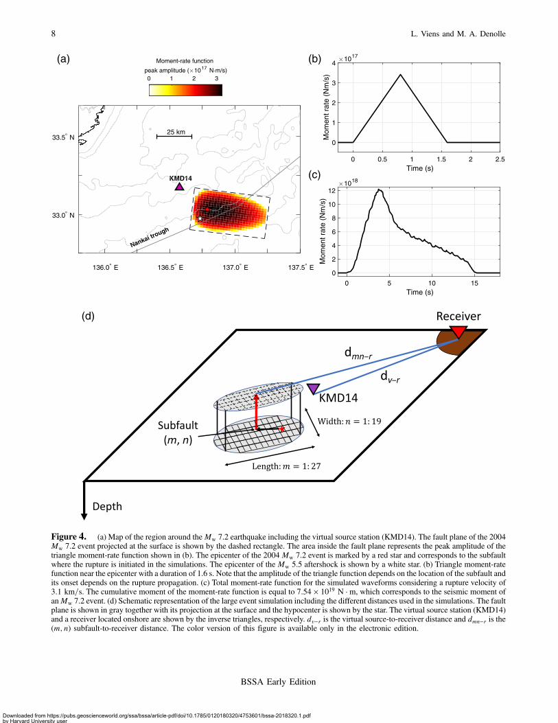
Figure 4. (a) Map of the region around theMw 7.2 earthquake including the virtual source station (KMD14). The fault plane of the 2004Mw 7.2 event projected at the surface is shown by the dashed rectangle. The area inside the fault plane represents the peak amplitude of thetriangle moment-rate function shown in (b). The epicenter of the 2004 Mw 7.2 event is marked by a red star and corresponds to the subfaultwhere the rupture is initiated in the simulations. The epicenter of the Mw 5.5 aftershock is shown by a white star. (b) Triangle moment-ratefunction near the epicenter with a duration of 1.6 s. Note that the amplitude of the triangle function depends on the location of the subfault andits onset depends on the rupture propagation. (c) Total moment-rate function for the simulated waveforms considering a rupture velocity of3:1 km=s. The cumulative moment of the moment-rate function is equal to 7:54 × 1019 N · m, which corresponds to the seismic moment ofanMw 7.2 event. (d) Schematic representation of the large event simulation including the different distances used in the simulations. The faultplane is shown in gray together with its projection at the surface and the hypocenter is shown by the star. The virtual source station (KMD14)and a receiver located onshore are shown by the inverse triangles, respectively. dv−r is the virtual source-to-receiver distance and dmn−r is the(m; n) subfault-to-receiver distance. The color version of this figure is available only in the electronic edition.


BSSA Early Edition


from worldwide subduction-zone earthquakes, includingJapanese earthquakes. In this section, we briefly describethe different parameters considered in our study and referthe reader to the original paper (e.g., Abrahamson et al.,2016) for additional details.

The BC Hydro GMM is composed of two functionalforms that have been determined from the regression analysisof records from interface and intraplate earthquakes. For the2004Mw 7.2 earthquake, we use the intraslab event functionalform and consider that our stations are located in the fore-arcregion. The intraslab GMM has a site amplification compo-nent that is based on VS30, the average S-wave velocity inthe upper 30 m of the ground. As Hi-net stations are locatedin relatively deep boreholes (100–3000 m depth), we use theborehole information provided on the KiK-net website todetermine the S-wave velocity in the borehole at the depthof each station, and set the VS30 parameter to this value. Theaverage S-wave velocity in the boreholes over the 60 Hi-netstations is 1458 m=s. For the stations with S-wave velocitieshigher than 1000 m=s, the VS30 parameter is set to 1000 m=sfollowing the GMM formulation. For intraslab events, the BCHydro model also considers the hypocentral distance, which isset accordingly to the hypocentral location in Table 1. To esti-mate the epistemic uncertainty in the median ground motionrelated to the break in magnitude scaling for Mw 8+ events,Abrahamson et al. (2016) introduced the ΔC1 term, which isset to −0:3 for intraplate events.

For the virtual Mw 8.0 megathrust earthquake, the inter-face event functional form of the BC Hydro GMM is con-sidered. We also consider that all stations are located in the

fore-arc region and use the same site conditions as for theintraplate event. The distance parameter of the interface func-tional form is the closest distance between site and faultplane. Therefore, we set this distance to be the distancebetween each receiver station and the center of the closestsubfault. For interface events, we use values of ΔC1 of−0:4, −0:2, and 0.0 to capture the model’s epistemic uncer-tainties as recommended by Abrahamson et al. (2016).

Waveform Comparison

To compare the simulated and observed waveforms, weuse several metrics that quantify the differences in phase,amplitude, and response spectra. The correlation coefficient(CC) allows us to compare seismic phases and is computedfor each component as

EQ-TARGET;temp:intralink-;df1;313;241CC �PN92:5

t�N2:5St × Et��PN92:5

t�N2:5S2t ×

PN92:5t�N2:5

E2t

q ; �1�

in which Et and St are the observed and simulated velocitywaveforms, respectively. N2:5 and N92:5 correspond to thetimes at which 2.5% and 92.5% of the cumulative energy ofboth signals (sum of the time-series values squared) isreached. We allow a 2 s time shift of the simulated wave-forms to maximize CC as the locations of the Mw 5.5 andMw 7.2 earthquakes are not well constrained (e.g., distancesbetween the epicenter of the Mw 7.2 event used in this studyand those listed in Table 1 vary between 3.5 and 40 km).Additional work, which is not the scope of the study, coulduse this fitting approach to do earthquake relocation.

50 km

Nankai trough

Hi-net DONET 1 DONET 2

135.0° E 135.5° E 136.0° E 136.5° E 137.0° E 137.5° E32.5° N

33.0° N

33.5° N

34.0° N

1 2 3 4

Moment-rate function

peak amplitude ( 1017 N·m/s)

0 5 10 15 20 25 30 35 40 45

Time (s)

0

1

2

3

4

5

6

7

8

9

Mom

ent r

ate

(Nm

/s)

1019

(a) (b)

Rupture velocity: 3.0 km/sRupture velocity: 2.5 km/sRupture velocity: 2.0 km/s

Figure 5. (a) Map of the Nankai subduction zone including the fault plane of a virtualMw 8.0 earthquake (dashed rectangle) determinedusing the oceanic reverse-faulting scaling relationships from Blaser et al. (2010). The area inside the fault plane represents the peak amplitudeof the triangle moment-rate function used for each subfault. The virtual source station (e.g., KMD14 station) is shown by the large triangleand the other DONET 1 stations, 20 of 29 DONET 2 stations, and a few Hi-net are represented by triangles. The star near the KMD14 stationis the epicenter of theMw 8.0 event and the epicenter of theMw 5.5 event is shown by a white star. (b) Total moment-rate functions for rupturevelocities of 2.0, 2.5, and 3:0 km=s. The color version of this figure is available only in the electronic edition.


BSSA Early Edition


The amplitude difference between the simulated andobserved waveforms is evaluated by computing the residualsof the long-period (4–10 s) PGVs for each component as

EQ-TARGET;temp:intralink-;df2;55;697Rj � ln�PGVsimj

PGVobsj

�; �2�

in which PGVobs and PGVsim are the observed and simulatedlong-period PGVs at the jth station, respectively, and ln isthe natural logarithm.

We finally compute the 5% damped SA values for theobserved and simulated waveforms at periods between 4and 10 s. The velocity time series are first differentiated oncein time to retrieve the corresponding acceleration waveformsand their response spectra are computed using the Duhamel’sintegral technique (Chopra, 2015). For each period τi andeach component, we compute the residuals between theobserved and simulated SA values Bj�τi� as

EQ-TARGET;temp:intralink-;df3;55;528Bj�τi� � ln�Asj�τi�Aej�τi�

�; �3�

in which Aej and Asj are the observed and simulated SAvalues at the jth station, respectively. The mean of the SAresiduals is computed by averaging the residuals over theconsidered number of stations N (e.g., 60 stations) as

EQ-TARGET;temp:intralink-;df4;55;433M�τi� �1

N

Xj�1;N

Bj�τi�: �4�

To quantify the variability of the mean of the SA residuals,we also compute the 90% confidence interval and the onestandard deviation to the mean for each component and eachperiod.

As the BC Hydro GMM was developed for the SA ofhorizontal components, we compute the geometric mean ofthe horizontal components for the observed (He�τ�) andsimulated (Hs�τ�) SA values at each period τ as

EQ-TARGET;temp:intralink-;df5;55;287

He�τ� ��AeT�τ� × AeR�τ�

q

Hs�τ� ��AsT�τ� × AsR�τ�

q; �5�

in which AeT�τ�, AeR�τ�, AsT�τ�, and AsR�τ� are theobserved (Ae) and simulated (As) SA values at a specificperiod τ with the component indicated by the superscript,with T for transverse and R for radial.

As the SA values of the BC Hydro GMM are in units ofg, we simply multiply them by the standard gravity value(e.g., 980:665 cm=s2) to retrieve the corresponding valuesin cm=s2. The residuals between the geometric mean ofthe observed and simulated SA waveforms as well as theresiduals between the GMM values and the geometric meanof the observed SA waveforms are then computed usingequation (3) and averaged using equation (4).

Results

Simulation of the 2004 Mw 5.5 Event

We show the simulated and observed velocity wave-forms in the 4–10 s period range for five stations located inthe direction of Osaka city from the earthquake source (loca-tion in Fig. 1) in Figure 6a–c. At these stations, the wave-forms exhibit relatively strong and elongated long-periodsurface waves compared to those from moderate crustalearthquakes in California (Denolle et al., 2013) and Japan(Viens, Miyake, et al., 2016). Because of the long durationof the ground motions, the CCs between the simulated andobserved waveforms tend to be low, but the main wave pack-ets can generally be retrieved for the three components. Forthe five stations shown in Figure 6a–c, the simulated andobserved long-period PGVs agree relatively well. There isalmost no basin amplification at the KNHH station as thestation is located in a 2-kilometer-deep borehole on the bed-rock of the Osaka basin. Finally, the simulated waveformsare mainly composed of surface waves and do not reproducewell the body waves from the earthquake (e.g., waves trav-eling faster than 3:0 km=s). However, in the 4–10 s periodrange and at relatively large distances from the epicenter,body waves tend to have smaller amplitudes than surfacewaves as shown in Figure 6a–c. This feature can beexplained by a stronger geometrical spreading of body wavescompared to surface waves as well as a stronger effect of theaccretionary wedge on surface waves as shown by physics-based simulations (e.g., Furumura et al., 2008; Yoshimuraet al., 2008; Guo et al., 2016).

Over the 60 Hi-net stations, the residuals of the long-period PGVs computed using equation (2) are distributedaround zero (mean values of 0.00, −0:07, and 0.00) and theirstandard deviations to the mean are relatively low with valuesof 0.35, 0.26, and 0.35 for the transverse, radial, and verticalcomponents, respectively (Fig. 6d–f). Moreover, for the60 Hi-net stations and the three components, 175 ratiosbetween observed and simulated long-period PGVs (e.g.,PGVsim=PGVobs) are within a factor of 2, and only 5 ratiosexhibit values beyond 2 but within a factor of 3. This sug-gests that the long-period PGVs are relatively well simulatedfor this earthquake. Finally, there are slight variations withdistance of the long-period PGV residuals for the transverseand vertical components for distances shorter than 175 kmfrom the virtual source. A possible explanation for this biasis that the surface-wave geometrical spreading correctionscheme applied to the IRFs is not appropriate for short dis-tances. Another explanation is that the earthquake location isnot accurate. Nevertheless, the average path may becomemore similar for longer distances and yields a distributionof the long-period PGV residuals around the zero bias forthe three components.

The 5% damped acceleration spectra of the simulatedand observed waveforms for the three components at threestations (e.g., SSRH, YOKH, and KTDH, location in Fig. 1)


BSSA Early Edition


are shown in Figure 7a–c. We selected these stations tosample different azimuths from the epicenter. For thesestations, the simulations reproduce relatively well the ob-served SAs in the 4–10 s period range. The accelerationspectra computed from the observed and simulated wave-forms are more complex than those from the BC HydroGMM. For each component, we compute the mean of theSA residuals over the 60 Hi-net stations and show it togetherwith the 90% confidence interval and one standard deviationto the mean values in Figure 7d. In the 4–10 s period range,the mean is generally distributed around zero despite small

but nonnegligible variations. However, the zero bias isalways within one standard deviation to the mean, indicatingthat the simulated waveforms reproduce relatively well thelong-period ground motions generated by the Mw 5.5earthquake.

Simulation of the 2004 Mw 7.2 Earthquake

Using the same illustration as for theMw 5.5 earthquake,we show the comparison between the velocity waveforms forthe 2004 Mw 7.2 earthquake in Figure 8a–c. Similar to the

Figure 6. Comparison between the simulated and observed velocity waveforms for the (a) transverse, (b) radial, and (c) vertical com-ponents for five stations located in the source-to-Osaka city axis (location in Fig. 1). All the waveforms are band-pass filtered between 4 and10 s. For each station, the correlation coefficient (CC) between the waveforms is indicated within parenthesis. Gray dashed lines represent the3:0 km=s moveout. (d–f) Long-period PGV residuals computed using equation (2) for the (d) transverse, (e) radial, and (f) vertical com-ponents as a function of the distance to the epicenter. Circles indicate that the ratio between the simulated and observed PGVs is within afactor of 2 and the squares represent ratio values larger than a factor of 2 but within a factor of 3. The black thick line is the mean of the data,and the 1 and 2 standard deviations to the mean are shown by the dark gray and light gray areas, respectively. For each panel, the mean of theresiduals (μ) and the standard deviation to the mean (σ) value are also indicated. The color version of this figure is available only in theelectronic edition.


BSSA Early Edition


moderate event, the duration of the strong long-periodground motions is relatively long for all the stations, and theCCs are relatively low due to the complex wave propagationthrough the accretionary prism. Nonetheless, the recordedwave packets with the largest amplitudes are generally wellreproduced by the simulated waveforms. We show the resid-uals of the long-period PGVs for the 60 Hi-net stations as a

function of the distance to the epicenter in Figure 8d–f. Forthe transverse, radial, and vertical components, the means ofthe residuals are 0.24, −0:01, and −0:09, and the standarddeviations to the mean are 0.39, 0.34, and 0.34, respectively.Moreover, we no longer observe any trend in the residualswith the distance from the epicenter, indicating that the crudegeometrical spreading correction was more problematic in

Figure 7. Simulated and observed 5% damped acceleration spectra for theMw 5.5 earthquake at the (a) SSRH, (b) YOKH, and (c) KTDHstations for the transverse, radial, and vertical components. For the two horizontal components, the intraplate functional form of the BCHydro ground-motion model (GMM) considering the hypocenter-to-receiver distance and the site conditions at each station is shown by adashed line. (d) Spectral acceleration (SA) residuals over the 60 Hi-net stations computed using equation (3) for theMw 5.5 earthquake. Foreach panel in (d), the mean of the SA residuals is shown together with the 90% confidence interval to the mean (dark gray area) and the onestandard deviation to the mean (light gray area). The zero bias line is highlighted with a black line. The color version of this figure is availableonly in the electronic edition.


BSSA Early Edition


the point-source case, but that the averaging over the faultplane reduces its effect. We also plot the residuals of thelong-period PGVs as a function of the azimuth from theepicenter in Figure 8g–i to show the lack of systematic

azimuthal variations. This indicates that the simple ellipticslip model used to simulate the long-period ground motionsreproduces relatively well the observed ground motions ofthe large intraplate seismic event.

Figure 8. (a–f) Same as Figure 6a–f for the 2004Mw 7.2 earthquake. (g–i) Long-period PGV residuals as a function of the azimuth fromthe epicenter (zero azimuth is north). Circles indicate that the ratio between simulated and observed PGVs are within a factor of 2 and thesquares represent values larger than a factor of 2 but within a factor of 3. The color version of this figure is available only in the electronicedition.


BSSA Early Edition


We also show the SA values between 4 and 10 s for thethree components at the SSRH, YOKH, and KTDH stationsin Figure 9a–c. Similar to the Mw 5.5 event, the simulatedand observed acceleration spectra for these three stationshave similar shapes in the 4–10 s period range. Moreover,the acceleration spectra from the simulated waveforms repro-duce better the observed ones compared to those from the BCHydro GMM. We also show the SA residuals computed overthe 60 Hi-net stations in Figure 9d for the three components.For the two horizontal components, the zero bias is within orclose to the 90% confidence interval to the mean, and alwayswithin one standard deviation to the mean in the 4–10 s

period range. For the vertical component, the average accel-eration spectra of the simulated waveforms slightly under-estimate those from the observed ground motions atperiods between 5 and 6 s, because the zero bias is slightlyoutside one standard deviation to the mean. For periodslonger than 6 s, the mean of the residuals becomes muchcloser to the zero bias.

In Figure 10, we show the residuals calculated betweenthe observed and simulated SA values averaged over the twohorizontal components using equation (5). The SA residualsare close to the zero bias as discussed earlier. We also showthe residuals computed between the observed and GMM SA

Figure 9. Same as Figure 7 for the 2004 Mw 7.2 earthquake. The color version of this figure is available only in the electronic edition.


BSSA Early Edition


values at discrete periods of 4, 5, 6, 7.5, and 10 s. The GMMdoes not perform well as the zero bias is outside one standarddeviation to the mean for periods of 4 and 10 s, indicatingthat the GMM overpredicts the observed SA values at theseperiods. One of the reasons of this bias at periods of 4 and10 s is the band-pass filter applied to the observed wave-forms, which reduces the amplitude of the SA values atthese periods. We also show in Figure 10 the mean of theSA residuals computed with unfiltered recorded waveforms.Although the effect of the band-pass filter is nonnegligible,the GMM SA values at 4 and 10 s still overpredict theobserved unfiltered waveforms. Therefore, our simulationsperform better than the BC Hydro GMM for the 2004Mw 7.2 earthquake in the 4–10 s period range.

Long-Period Ground Motions from a Virtual Mw 8.0Megathrust Event

Finally, we predict the long-period ground motions of ahypothetical Mw 8.0 subduction event for rupture velocitiesof 2.0, 2.5, and 3:0 km=s and show their horizontal wave-forms at the KHOH and KNHH stations in Figure 11a–d.Unsurprisingly, the level of the long-period ground motionincreases with the increasing rupture velocity, as expectedthat faster ruptures generate stronger ground motions.

We show the 5% damped SA values at 5, 6, and 7.5 scomputed from the simulated waveforms for the three rupturevelocities as a function of the distance from the closest sub-fault where slip occurred to each receiver station (equivalent toRrup distance in the BC Hydro GMM) in Figure 11e–l. For theperiods of interest, we observe a general decay of the SA

values with increasing distance from the source and an in-crease of the SA values with increasing rupture velocity. Wealso show the SA values from the plate-interface event BCHydro GMM in Figure 11e–l. As the rupture velocity is notaccounted in the GMMs, the GMM predictions are invariantwith respect to rupture velocity in this exercise. However,because this parametric function was determined from ob-served ground motions, it should account for realistic rupturevelocities of megathrust events. Overall, the GMM SA valuesdecay with increasing periods, whereas the virtual megathrustSA values remain constant, if not slightly amplified. This isconsistent with the results for theMw 7.2 earthquake, in whichthe simulated and observed waveforms remain constant withincreasing periods from 5 to 7.5 s (Ⓔ Fig. S9). For a rupturevelocity of 2:0 km=s, the SA values from our simulations arelower than those from the GMM at a period of 5 s, and com-parable at periods of 6 and 7.5 s. For a 3:0 km=s rupturevelocity, our simulations have SA values higher than thosefrom the GMM for the three periods. For a rupture velocityof 2:5 km=s, a commonly reported value for subduction-zoneearthquakes, the agreement between the SA values is good at5 s and our simulations have higher values than the GMMat periods of 6 and 7.5 s. Therefore, for a hypothetical Mw

8.0 subduction event with a rupture velocity of 2:5 km=s orhigher, our simulations show that the long-period groundmotions at periods of 5, 6, and 7.5 are likely to be higher thanthose expected with the BC Hydro GMM.

The Hi-net stations are located in deep boreholes on thebedrock, and therefore a linear response of the surroundingmaterial is expected. However, for stations located at the sur-face of sedimentary basins composed of almost cohesionlessmaterials, one might expect a nonlinear response of the basinthat could reduce long-period shaking levels as shown by thesimulations performed by Roten et al. (2014).

Conclusions

In this study, we simulated the long-period groundmotions of subduction-zone earthquakes using the ambientseismic field. We first retrieved IRFs between an offshoreDONET station (KMD14) and onshore Hi-net stations usingseismic interferometry by deconvolution. We then convolvedthe IRFs with a triangle source time function to simulate thevelocity ground motions of a moderate Mw 5.5 earthquake,which is approximated as a point source. As only the relativeamplitude of the IRFs is retrieved with the deconvolutiontechnique, we computed a calibration factor for each compo-nent of the IRFs using the records of theMw 5.5 event. Afteramplitude calibration, we compared the simulated andobserved velocity waveforms and found that the observedground motions do not carry the signature of any radiationpattern effects in the 4–10 s period range. This indicates thatthe long-period ground motions recorded onshore are likelymore affected by the wave propagation through the accre-tionary wedge than by source effects. This feature allowed

Figure 10. Comparison between the mean and the 1 standarddeviation (st. dev.) to the mean of the SA residuals computedbetween the band-pass filtered Mw 7.2 earthquake records andthe simulations and between the band-pass filtered Mw 7.2 earth-quake records and the BC Hydro GMM. The mean of the SA resid-uals computed from the unfiltered 2004Mw 7.2 earthquake recordsand the BC Hydro GMM is shown by the dashed line. The zero biasis highlighted with a black line. The color version of this figure isavailable only in the electronic edition.


BSSA Early Edition


0 50 100 150 200 250 300

Time (s)

–10

–5

0

5

10V

eloc

ity (

cm/s

)

Mw 8.0 predictionKHOH station

Transverse component(a)

Rupture velocity: 3.0 km/sRupture velocity: 2.5 km/sRupture velocity: 2.0 km/s

0 50 100 150 200 250 300

Time (s)

–10

–5

0

5

10

Vel

ocity

(cm

/s)

Mw 8.0 predictionKHOH station

Radial component(b)

0 50 100 150 200 250 300Time (s)

–2

–1

0

1

2

Vel

ocity

(cm

/s)

KNHH stationTransverse component

(c)

0 50 100 150 200 250 300Time (s)

–2

–1

0

1

2

Vel

ocity

(cm

/s)

KNHH stationRadial component

(d)

50 100 150 200 250

Distance to the closest subfault (km)

100

101

102

Spe

ctra

l acc

eler

atio

n (c

m/s

2)

Rupture velocity: 2 km/sSA 5 s (h = 5%)

(e)

50 100 150 200 250


100

101

102

Spe

ctra

l acc

eler

atio

n (c

m/s

2)

SA 6 s (h = 5%)(f)

50 100 150 200 250


100

101

102

Spe

ctra

l acc

eler

atio

n (c

m/s

2)

SA 7.5 s (h = 5%)(g)

50 100 150 200 250


Rupture velocity: 2.5 km/sSA 5 s (h = 5%)

(h)

50 100 150 200 250


SA 6 s (h = 5%)(i)

BC Hydro C1 = 0.0BC Hydro C1 = –0.2BC Hydro C1 = –0.4Simulation

50 100 150 200 250


SA 7.5 s (h = 5%)(j)

50 100 150 200 250


100

101

102

Rupture velocity: 3 km/sSA 5 s (h = 5%)

(k)

50 100 150 200 250


100

101

102SA 6 s (h = 5%)

(l)

50 100 150 200 250


100

101

102SA 7.5 s (h = 5%)

(m)

Figure 11. (a–d) Simulated velocity waveforms for the transverse and radial components at the KHOH and KNHH stations for a hypo-thetical Mw 8.0 subduction earthquake. For each panel, the waveforms are simulated considering constant rupture velocities of 2.0, 2.5, and3:0 km=s. All waveforms are band-pass filtered between 4 and 10 s. (e–l) 5% damped SAvalues at periods of 5, 6, and 7.5 s from the medianBC Hydro GMM (Abrahamson et al., 2016) and from our simulations (circles) considering rupture velocities of (e–g) 2.0, (h–j) 2.5, and(k–m) 3:0 km=s for the hypotheticalMw 8.0 subduction earthquake. All the SA values are shown as a function of the distance to the closestsubfault where slip occurs. For each panel, three values of the ΔC1 parameter are shown for the BC Hydro GMM (VS30 � 1000 m=s), whichare set to capture the epistemic uncertainties. The color version of this figure is available only in the electronic edition.


BSSA Early Edition


us to simplify the simulations and to generalize the predic-tions by simply using minimal transformation of the IRFs.

We further compared the simulated and observed veloc-ity waveforms of the moderate Mw 5.5 intraplate earthquakeusing several metrics. We showed that the simulated andobserved waveforms have similar wave packets and thatlong-period PGVs agree well in the 4–10 s period range.Moreover, the analysis of the SA values demonstrated thatthe spectral content of the observed and simulated wave-forms is relatively similar in the period range of interest.

We then constructed a finite-fault elliptic slip sourcemodel of the 2004 Mw 7.2 intraplate earthquake, whichwas inspired by previously reported finite-fault inversions.By combining the amplitude-calibrated IRFs and the sourcemodel, we simulated the long-period ground motions of thisevent. For a constant rupture velocity of 3:1 km=s, our sim-ulations reproduced well the observed waveforms in terms ofphase, amplitude, and SA in the 4–10 s period range. We alsocross-validated our results with the BC Hydro GMM andshowed an improved performance in the predictions withour approach in the period range of interest.

We finally predicted the long-period ground motions ofa hypothetical Mw 8.0 megathrust event that could occuralong the Nankai subduction zone with an elliptic slip sourcemodel. Although the source model considered in this study isvery simple, the SA values from the simulated waveformsusing rupture velocities of 2:5 km=s or higher are larger thanthose computed from the BC Hydro GMM at periods of 5, 6,and 7.5 s. In future work, the simulations will be improved tobetter assess the seismic hazard related to the long-periodground motions from hypothetical megathrust events thatcould occur along the Nankai trough. This could be done byincluding multiple virtual source stations from the DONET 1and 2 networks to better capture the 3D wave propagationfrom different parts of the fault. Moreover, realistic kin-ematic source models should be used to infer the long-periodground-motion variability related to Mw 8+ megathrustevents in this region. Finally, future work should explorefurther data-processing techniques to improve the SNR ofoffshore–onshore IRFs, as ocean-bottom seismometer datahave relatively high noise levels at periods longer than 5 s(Crawford and Webb, 2000; Webb and Crawford, 2010).

With the increasing number of offshore and onshore net-works, the ambient seismic-field-based method could beapplied to different subduction zones worldwide to simulateand predict the long-period ground motions of past andfuture megathrust earthquakes. For example, the Cascadia,Costa Rica, and Alaska subduction zones also benefit frommultiyear offshore arrays that could be used to performsimilar long-period ground-motion predictions of megathrustevents. Such results could be coupled to those from othertechniques such as physics-based simulations and GMMsto better assess seismic hazard related to offshore subductionearthquakes.

Data and Resources

Both the Hi-net and Dense Oceanfloor Network Systemfor Earthquakes and Tsunamis (DONET) data can be down-loaded at http://www.hinet.bosai.go.jp. Information aboutearthquakes is from the Japan Meteorological Agency (JMA)and F-net/National Research Institute for Earth Science andDisaster Resilience (NIED). The borehole data at Hi-net sta-tions can be found on the KiK-net/NIED website at http://www.kyoshin.bosai.go.jp. The Python and MATLAB codesused in this study to compute the impulse response functions(IRFs), to simulate the Mw 7.2 event, and to compute accel-eration response spectra are available at https://github.com/lviens. All websites were last accessed on May 2019.

Acknowledgments

The authors are grateful to Hiroe Miyake for helpful dis-cussions about this study. The authors thank Associate EditorArben Pitarka and two anonymous reviewers for theirdetailed and constructive comments. This work is supportedby National Science Foundation (NSF) Award NumberEAR-1663827. L. V. is currently supported by the JapanSociety for the Promotion of Science Fellowship. Theauthors acknowledge the National Research Institute forEarth Science and Disaster Resilience (NIED) for providingthe Hi-net data and Japan Agency for Marine-Earth Scienceand Technology (JAMSTEC) for the Dense OceanfloorNetwork System for Earthquakes and Tsunamis (DONET)data. The authors also thank the Japan MeteorologicalAgency (JMA) and F-net/NIED for providing informationabout earthquakes, and KiK-net/NIED for the borehole infor-mation data. The authors are grateful to Ryo Okuwaki forproviding the source model of the 2004 Mw 7.2 earthquake.

References

Abrahamson, N., N. Gregor, and K. Addo (2016). BC Hydro ground motionprediction equations for subduction earthquakes, Earthq. Spectra 32,23–44, doi: 10.1193/051712EQS188MR.

Anderson, J. G., P. Bodin, J. N. Brune, J. Prince, S. K. Singh, R. Quaas, andM. Onate (1986). Strong ground motion from the Michoacan,Mexico, earthquake, Science 233, 1043–1049, doi: 10.1126/sci-ence.233.4768.1043.

Ando, M. (1975). Source mechanisms and tectonic significance of historicalearthquakes along the Nankai trough, Japan, Tectonophysics 27, 119–140, doi: 10.1016/0040-1951(75)90102-X.

Atkinson, G. M., and D. M. Boore (2003). Empirical ground-motion rela-tions for subduction-zone earthquakes and their application toCascadia and other regions, Bull. Seismol. Soc. Am. 93, 1703, doi:10.1785/0120020156.

Atkinson, G. M., and D. M. Boore (2008). Erratum to empirical ground-motion relations for subduction zone earthquakes and their applicationto Cascadia and other regions, Bull. Seismol. Soc. Am. 98, 2567, doi:10.1785/0120080108.

Bai, L., E. A. Bergman, E. R. Engdahl, and I. Kawasaki (2007). The 2004earthquakes offshore of the Kii peninsula, Japan: Hypocentral reloca-tion, source process and tectonic implication, Phys. Earth Planet. In.165, 47–55, doi: 10.1016/j.pepi.2007.07.007.

BC Hydro (2012). Probabilistic seismic hazard analysis (PSHA) model, BCHydro Engineering Report E658, Vancouver.


BSSA Early Edition


http://www.hinet.bosai.go.jp





http://www.kyoshin.bosai.go.jp

http://www.kyoshin.bosai.go.jp

https://github.com/lviens

https://github.com/lviens

http://dx.doi.org/10.1193/051712EQS188MR

http://dx.doi.org/10.1126/science.233.4768.1043

http://dx.doi.org/10.1126/science.233.4768.1043

http://dx.doi.org/10.1016/0040-1951(75)90102-X

http://dx.doi.org/10.1785/0120020156

http://dx.doi.org/10.1785/0120080108

http://dx.doi.org/10.1016/j.pepi.2007.07.007

Beck, J. L., and J. F. Hall (1986). Factors contributing to the catastrophe inMexico City during the earthquake of September 19, 1985, Geophys.Res. Lett. 13, 593–596, doi: 10.1029/GL013i006p00593.

Blaser, L., F. Krüger, M. Ohrnberger, and F. Scherbaum (2010). Scaling rela-tions of earthquake source parameter estimates with special focus onsubduction environment, Bull. Seismol. Soc. Am. 100, 2914–2926, doi:10.1785/0120100111.

Boué, P., M. Denolle, N. Hirata, S. Nakagawa, and G. C. Beroza (2016).Beyond basin resonance: Characterizing wave propagation using adense array and the ambient seismic field, Geophys. J. Int. 206,1261–1272, doi: 10.1093/gji/ggw205.

Bowden, D. C., V. C. Tsai, and F. C. Lin (2015). Site amplification, attenu-ation, and scattering from noise correlation amplitudes across a densearray in Long Beach, CA, Geophys. Res. Lett. 42, 1360–1367, doi:10.1002/2014GL062662.

Chopra, A. (2015). Dynamics of Structures, International Edition, PearsonEducation Limited, Harlow, United Kingdom.

Crawford, W. C., and S. C. Webb (2000). Identifying and removing tilt noisefrom low-frequency (<0:1 Hz) seafloor vertical seismic data, Bull.Seismol. Soc. Am. 90, 952, doi: 10.1785/0119990121.

Crawford, W. C., R. A. Stephen, and S. T. Bolmer (2006). A second look atlow-frequency marine vertical seismometer data quality at the OSN-1site off Hawaii for seafloor, buried, and borehole emplacements, Bull.Seismol. Soc. Am. 96, 1952, doi: 10.1785/0120050234.

Crouse, C. B., Y. K. Vyas, and B. A. Schell (1988). Ground motions fromsubduction-zone earthquakes, Bull. Seismol. Soc. Am. 78, 1.

Denolle, M. A., P. Boué, N. Hirata, and G. C. Beroza (2018). Strongshaking predicted in Tokyo from an expected M7+ Itoigawa-Shizuoka earthquake, J. Geophys. Res. 123, 3968–3992, doi:10.1029/2017JB015184.

Denolle, M. A., E. M. Dunham, G. A. Prieto, and G. C. Beroza (2013).Ground motion prediction of realistic earthquake sources using theambient seismic field, J. Geophys. 118, 2102–2118, doi: 10.1029/2012JB009603.

Denolle, M. A., E. M. Dunham, G. A. Prieto, and G. C. Beroza (2014).Strong ground motion prediction using virtual earthquakes, Science343, 399–403, doi: 10.1126/science.1245678.

Eshelby, J. (1957). The determination of the elastic field of an ellipsoidalinclusion, and related problems, Proc. Math. Phys. Sci. 241, 376–396, doi: 10.1098/rspa.1957.0133.

Furumura, T., T. Hayakawa, M. Nakamura, K. Koketsu, and T. Baba (2008).Development of long-period ground motions from the Nankai trough,Japan, earthquakes: Observations and computer simulation of the 1944Tonankai (Mw 8.1) and the 2004 SE Off-Kii Peninsula (Mw 7.4) earth-quakes, Pure Appl. Geophys. 165, 585–607, doi: 10.1007/s00024-008-0318-8.

Guo, Y., K. Koketsu, and H. Miyake (2016). Propagation mechanism oflong-period ground motions for offshore earthquakes along theNankai trough: Effects of the accretionary wedge, Bull. Seismol.Soc. Am. 106, 1176–1197, doi: 10.1785/0120150315.

Kaneda, Y., K. Kawaguchi, E. Araki, H. Matsumoto, T. Nakamura, S.Kamiya, K. Ariyoshi, T. Hori, T. Baba, and N. Takahashi (2015).Development and application of an advanced ocean floor networksystem for megathrust earthquakes and tsunamis, in SeafloorObservatories, P. Favali, L. Beranzoli, and A. De Santis (Editors),Springer Berlin Heidelberg, Berlin/Heidelberg, Germany, 643–662.

Kawaguchi, K., S. Kaneko, T. Nishida, and T. Komine (2015). Constructionof the DONET real-time seafloor observatory for earthquakes and tsu-nami monitoring, in Seafloor Observatories, P. Favali, L. Beranzoli,and A. De Santis (Editors), Springer Berlin Heidelberg, Berlin/Heidelberg, Germany, 211–228.

Koketsu, K., K. Hatayama, T. Furumura, Y. Ikegami, and S. Akiyama(2005). Damaging long-period ground motions from the 2003Mw 8.3 Tokachi-oki, Japan earthquake, Seismol. Res. Lett. 76, 67–73, doi: 10.1785/gssrl.76.1.67.

Koketsu, K., H. Miyake, Afnimar, and Y. Tanaka (2009). A proposal for astandard procedure of modeling 3-D velocity structures and its

application to the Tokyo metropolitan area, Japan, Tectonophysics472, 290–300, doi: 10.1016/j.tecto.2008.05.037.

Koketsu, K., H. Miyake, H. Fujiwara, and T. Hashimoto (2008). Progresstowards a Japan integrated velocity structure model and long-periodground motion hazard map, Proc. of the 14th World Conf. onEarthquake Engineering, Beijing, China, 12–17 October 2008,S10–038.

Koketsu, K., H. Miyake, and H. Suzuki (2012). Japan integrated velocitystructure model version 1, Proc. of the 15th World Conf. onEarthquake Engineering, Lisbon, Portugal, 24–28 September, 1773.

Kwak, S., S. G. Song, G. Kim, C. Cho, and J. S. Shin (2017). Investigatingthe capability to extract impulse response functions from ambientseismic noise using a mine collapse event, Geophys. Res. Lett. 44,9653–9662, doi: 10.1002/2017GL075532.

Lawrence, J. F., and G. A. Prieto (2011). Attenuation tomography of thewestern United States from ambient seismic noise, J. Geophys. Res.116, no. B06302, doi: 10.1029/2010JB007836.

Lawrence, J. F., M. Denolle, K. J. Seats, and G. A. Prieto (2013). A numericevaluation of attenuation from ambient noise correlation functions, J.Geophys. Res. 118, 6134–6145, doi: 10.1002/2012JB009513.

Lin, F.-C., M. P. Moschetti, and M. H. Ritzwoller (2008). Surface wavetomography of the western United States from ambient seismic noise:Rayleigh and Love wave phase velocity maps, Geophys. J. Int. 173,281–298, doi: 10.1111/j.1365-246X.2008.03720.x.

Liu, X., Y. Ben-Zion, and D. Zigone (2016). Frequency domain analysis oferrors in cross-correlations of ambient seismic noise, Geophys. J. Int.207, 1630–1652, doi: 10.1093/gji/ggw361.

Miyake, H., and K. Koketsu (2005). Long-period ground motions from alarge offshore earthquake: The case of the 2004 off the Kii peninsulaearthquake, Japan, Earth Planets Space 57, 203–207, doi: 10.1186/BF03351816.

Nakano, M., T. Tonegawa, and Y. Kaneda (2012). Orientations of DONETseismometers estimated from seismic waveforms, JAMSTEC Rep. Res.Dev. 15, 77–89.

Obara, K., K. Kasahara, S. Hori, and Y. Okada (2005). A densely distributedhigh-sensitivity seismograph network in Japan: Hi-net by NationalResearch Institute for Earth Science and Disaster Prevention, Rev.Sci. Instrum. 76, 021301, doi: 10.1063/1.1854197.

Okada, Y., K. Kasahara, S. Hori, K. Obara, S. Sekiguchi, H. Fujiwara, andA. Yamamoto (2004). Recent progress of seismic observation net-works in Japan—Hi-net, F-net, K-NET and KiK-net, Earth PlanetsSpace 56, xv–xxviii, doi: 10.1186/BF03353076.

Okuwaki, R., and Y. Yagi (2018). rokuwaki/2004Mw7.2KiiJapan: v1.0, doi:10.5281/zenodo.1493833.

Park, S.-C., and J. Mori (2005). The 2004 sequence of triggered earthquakesoff the Kii peninsula, Japan, Earth Planets Space 57, 315–320, doi:10.1186/BF03352569.

Prieto, G. A., and G. C. Beroza (2008). Earthquake ground motion predic-tion using the ambient seismic field, Geophys. Res. Lett. 35, L14304,doi: 10.1029/2008GL034428.

Prieto, G. A., M. Denolle, J. F. Lawrence, and G. C. Beroza (2011). Onamplitude information carried by the ambient seismic field, Compt.Rendus Geosci. 343, 600–614, doi: 10.1016/j.crte.2011.03.006.

Roten, D., K. B. Olsen, S. M. Day, Y. Cui, and D. Fäh (2014). Expectedseismic shaking in Los Angeles reduced by San Andreas fault zoneplasticity, Geophys. Res. Lett. 41, 2769–2777, doi: 10.1002/2014GL059411.

Roux, P., K. G. Sabra, P. Gerstoft, W. A. Kuperman, and M. C. Fehler(2005). P-waves from cross-correlation of seismic noise, Geophys.Res. Lett. 32, L19303, doi: 10.1029/2005GL023803.

Sabra, K. G., P. Gerstoft, P. Roux, W. A. Kuperman, and M. C. Fehler(2005). Extracting time-domain Green’s function estimates from ambi-ent seismic noise, Geophys. Res. Lett. 32, L03310, doi: 10.1029/2004GL021862.

Shapiro, N. M., and M. Campillo (2004). Emergence of broadband Rayleighwaves from correlations of the ambient seismic noise, Geophys. Res.Lett. 31, L07614, doi: 10.1029/2004GL019491.


BSSA Early Edition


http://dx.doi.org/10.1029/GL013i006p00593

http://dx.doi.org/10.1785/0120100111

http://dx.doi.org/10.1093/gji/ggw205

http://dx.doi.org/10.1002/2014GL062662

http://dx.doi.org/10.1785/0119990121

http://dx.doi.org/10.1785/0120050234

http://dx.doi.org/10.1029/2017JB015184

http://dx.doi.org/10.1029/2012JB009603

http://dx.doi.org/10.1029/2012JB009603

http://dx.doi.org/10.1126/science.1245678

http://dx.doi.org/10.1098/rspa.1957.0133

http://dx.doi.org/10.1007/s00024-008-0318-8

http://dx.doi.org/10.1007/s00024-008-0318-8

http://dx.doi.org/10.1785/0120150315

http://dx.doi.org/10.1785/gssrl.76.1.67

http://dx.doi.org/10.1016/j.tecto.2008.05.037

http://dx.doi.org/10.1002/2017GL075532

http://dx.doi.org/10.1029/2010JB007836

http://dx.doi.org/10.1002/2012JB009513

http://dx.doi.org/10.1111/j.1365-246X.2008.03720.x

http://dx.doi.org/10.1093/gji/ggw361

http://dx.doi.org/10.1186/BF03351816

http://dx.doi.org/10.1186/BF03351816

http://dx.doi.org/10.1063/1.1854197

http://dx.doi.org/10.1186/BF03353076

http://dx.doi.org/10.5281/zenodo.1493833

http://dx.doi.org/10.1186/BF03352569

http://dx.doi.org/10.1029/2008GL034428

http://dx.doi.org/10.1016/j.crte.2011.03.006

http://dx.doi.org/10.1002/2014GL059411

http://dx.doi.org/10.1002/2014GL059411

http://dx.doi.org/10.1029/2005GL023803

http://dx.doi.org/10.1029/2004GL021862

http://dx.doi.org/10.1029/2004GL021862

http://dx.doi.org/10.1029/2004GL019491

Shapiro, N. M., M. Campillo, L. Stehly, and M. H. Ritzwoller (2005). High-resolution surface-wave tomography from ambient seismic noise,Science 307, 1615–1618, doi: 10.1126/science.1108339.

Shapiro, N. M., M. H. Ritzwoller, and G. D. Bensen (2006). Source locationof the 26 sec microseism from cross-correlations of ambient seismicnoise, Geophys. Res. Lett. 33, L18310, doi: 10.1029/2006GL027010.

Sheng, Y., M. A. Denolle, and G. C. Beroza (2017). Multicomponent C3Green’s functions for improved long-period ground-motion prediction,Bull. Seismol. Soc. Am. 107, 2836, doi: 10.1785/0120170053.

Shiomi, K. (2013). New measurements of sensor orientation at NIED Hi-netstations, Rep. NIED 80, 1–20.

Snieder, R. (2004). Extracting the Green’s function from the correlation ofcoda waves: A derivation based on stationary phase, Phys. Rev. E 69,046610, doi: 10.1103/PhysRevE.69.046610.

Somerville, P., K. Irikura, R. Graves, S. Sawada, D. Wald, N. Abrahamson,Y. Iwasaki, T. Kagawa, N. Smith, and A. Kowada (1999).Characterizing crustal earthquake slip models for the prediction ofstrong ground motion, Seismol. Res. Lett. 70, 59–80, doi: 10.1785/gssrl.70.1.59.

Stehly, L., and P. Boué (2017). On the interpretation of the amplitude decayof noise correlations computed along a line of receivers, Geophys. J.Int. 209, 358, doi: 10.1093/gji/ggx021.

Stutzmann, E., J.-P. Montagner, A. Sebai, W. C. Crawford, J.-L. Thirot, P.Tarits, D. Stakes, B. Romanowicz, J.-F. Karczewski, J.-C. Koenig, et al.(2001). Moise: A prototype multiparameter ocean-bottom station, Bull.Seismol. Soc. Am. 91, 885, doi: 10.1785/0120000035.

Suzuki, W., T. Iwata, K. Asano, and N. Yamada (2005). Estimation of thesource model for the foreshock of the 2004 off the Kii peninsula earth-quakes and strong ground motion simulation of the hypotheticalTonankai earthquake using the empirical Green’s function method,Earth Planets Space 57, 345–350, doi: 10.1186/BF03352574.

Takagi, R., K. Nishida, T. Maeda, and K. Obara (2018). Ambient seismicnoise wavefield in Japan characterized by polarization analysis ofHi-net records, Geophys. J. Int. 215, 1682–1699, doi: 10.1093/gji/ggy334.

The Headquarters for Earthquake Research Promotion (2013). Long-TermEvaluation of Nankai Trough Earthquake Activity, Second Ed., avail-able at https://www.jishin.go.jp/main/chousa/13may_nankai/index.htm (last accessed May 2018) (in Japanese).

Tsai, V. C. (2011). Understanding the amplitudes of noise correlationmeasurements, J. Geophys. Res. 116, no. B09311, doi: 10.1029/2011JB008483.

Viens, L., M. Denolle, H. Miyake, S. Sakai, and S. Nakagawa (2017).Retrieving impulse response function amplitudes from the ambientseismic field, Geophys. J. Int. 210, 210–222, doi: 10.1093/gji/ggx155.

Viens, L., K. Koketsu, H. Miyake, S. Sakai, and S. Nakagawa (2016). Basin-scale Green’s functions from the ambient seismic field recorded byMeSO-net stations, J. Geophys. Res. 121, 2507–2520, doi:10.1002/2016JB012796.

Viens, L., A. Laurendeau, L. F. Bonilla, and N. M. Shapiro (2014). Broad-band acceleration time histories synthesis by coupling low-frequency

ambient seismic field and high-frequency stochastic modelling,Geophys. J. Int. 199, 1784–1797, doi: 10.1093/gji/ggu362.

Viens, L., H. Miyake, and K. Koketsu (2015). Long-period ground motionsimulation of a subduction earthquake using the offshore-onshoreambient seismic field, Geophys. Res. Lett. 42, 5282–5289, doi:10.1002/2015GL064265.

Viens, L., H. Miyake, and K. Koketsu (2016). Simulations of long-periodground motions from a large earthquake using finite rupture modelingand the ambient seismic field, J. Geophys. Res. 121, 2507–2520, doi:10.1002/2016JB012796.

Watanabe, S., Y. Bock, D. Melgar, and K. Tadokoro (2018). Tsunami sce-narios based on interseismic models along the Nankai trough, Japan,from seafloor and onshore geodesy, J. Geophys. Res. 123, 2448–2461,doi: 10.1002/2017JB014799.

Weaver, R. L. (2011). On the amplitudes of correlations and the inference ofattenuations, specific intensities and site factors from ambient noise,Compt. Rendus Geosci. 343, 615–622, doi: 10.1016/j.crte.2011.07.001.

Webb, S. C., and W. C. Crawford (2010). Shallow-water broadband OBSseismology, Bull. Seismol. Soc. Am. 100, 1770, doi: 10.1785/0120090203.

Yagi, Y. (2004). On the earthquakes that occurred southeast off Kii peninsulaon September 5, 2004, available at https://www.kenken.go.jp/japanese/information/information/press/20040908.pdf (last accessedMay 2019) (in Japanese).

Yoshimura, C., Y. Yamamoto, and Y. Hisada (2008). Long-period groundmotion simulation of 2004 off the Kii peninsula earthquakes and pre-diction of future M8 class earthquakes along Nankai trough subductionzone, south of Japan Island, Proc. of the 14th World Conf. on Earthq.Eng., Beijing, China, 12–17 October 2008.

Youngs, R., S.-J. Chiou, W. Silva, and J. Humphrey (1997). Strong groundmotion attenuation relationships for subduction zone earthquakes,Seismol. Res. Lett. 68, 58, doi: 10.1785/gssrl.68.1.58.

Zeng, X., and S. Ni (2010). A persistent localized microseismic source nearthe Kyushu Island, Japan, Geophys. Res. Lett. 37, L24307, doi:10.1029/2010GL045774.

Zhao, J. X., J. Zhang, A. Asano, Y. Ohno, T. Oouchi, T. Takahashi, H.Ogawa, K. Irikura, H. K. Thio, P. G. Somerville, et al. (2006).Attenuation relations of strong ground motion in Japan using siteclassification based on predominant period, Bull. Seismol. Soc. Am.96, 898, doi: 10.1785/0120050122.

Department of Earth and Planetary SciencesHarvard University20 Oxford StreetCambridge, Massachusetts 02138 [email protected]‑u.ac.jp

Manuscript received 2 December 2018;Published Online 18 June 2019


BSSA Early Edition


http://dx.doi.org/10.1126/science.1108339

http://dx.doi.org/10.1029/2006GL027010

http://dx.doi.org/10.1785/0120170053

http://dx.doi.org/10.1103/PhysRevE.69.046610



http://dx.doi.org/10.1093/gji/ggx021

http://dx.doi.org/10.1785/0120000035

http://dx.doi.org/10.1186/BF03352574

http://dx.doi.org/10.1093/gji/ggy334

http://dx.doi.org/10.1093/gji/ggy334

https://www.jishin.go.jp/main/chousa/13may_nankai/index.htm





http://dx.doi.org/10.1029/2011JB008483

http://dx.doi.org/10.1029/2011JB008483

http://dx.doi.org/10.1093/gji/ggx155

http://dx.doi.org/10.1002/2016JB012796

http://dx.doi.org/10.1093/gji/ggu362

http://dx.doi.org/10.1002/2015GL064265

http://dx.doi.org/10.1002/2016JB012796

http://dx.doi.org/10.1002/2017JB014799

http://dx.doi.org/10.1016/j.crte.2011.07.001

http://dx.doi.org/10.1785/0120090203

http://dx.doi.org/10.1785/0120090203

https://www.kenken.go.jp/japanese/information/information/press/20040908.pdf







http://dx.doi.org/10.1029/2010GL045774

http://dx.doi.org/10.1785/0120050122

long-period ground motions from past and virtual

Documents