long-run economic growth - brad delong

Long-Run EconomicGrowth

P A R TII

Long-run economic growth is the subject of this two-chapter part.Chapter 4 covers the theory of growth, and Chapter 5 covers the world-wide pattern of economic growth. Long-run economic growth is themost important topic in macroeconomics. Standards of living in theUnited States today are at least five times what they were at the end ofthe nineteenth century. Successful economic growth has meant that al-most all citizens of the United States today live better, and we hopehappier, lives than even the rich elite of a century ago. The study oflong-run economic growth aims at understanding its sources and causesand at determining what government policies will promote or retardlong-run economic growth.

The study of long-run growth is also a separate module that is not veryclosely connected to the study of business cycles, recessions, unem-ployment, inflation, and stabilization policy that make up the bulk ofthe subject matter of macroeconomics courses and of this book. Anydiscussion of economic policy has to refer to long-run economic growth:The effect of a policy on long-run growth is its most important element.But the models used and the conclusions reached in Part II will by andlarge not be used in subsequent parts. Starting in Chapter 6, our at-tention turns from growth to business cycles.

Why, then, include this two-chapter part on long-rung growth? Theprincipal reason is that long-run economic growth is such an importanttopic that it must be covered.

QUESTIONS

What are the principal determinants of long-run economic growth?

What equilibrium condition is useful in analyzing long-run growth?

How quickly does an economy head for its steady-state growth path?

What effect does faster population growth have on long-run growth?

What effect does a higher savings rate have on long-run growth?

The Theory of Economic Growth

C H A P T E R4

4.1 SOURCES OF LONG-RUN GROWTH Ultimately, long-run economic growth is the most important aspect of how the econ-omy performs. Material standards of living and levels of economic productivity inthe United States today are about four times what they are today in, say, Mexico be-cause of favorable initial conditions and successful growth-promoting economicpolicies over the past two centuries. Material standards of living and levels of eco-nomic productivity in the United States today are at least five times what they wereat the end of the nineteenth century and more than ten times what they were at thefounding of the republic. Successful economic growth has meant that most citizensof the United States today live better, along almost every dimension of material life,than did even the rich elite in preindustrial times.

It is definitely possible for good and bad policies to accelerate or retard long-runeconomic growth. Argentines were richer than Swedes in the years before World WarI began in 1914, but Swedes today have perhaps four times the material standard ofliving and the economic productivity level of Argentines. Almost all this differenceis due to differences in growth policies — good policies in the case of Sweden, badpolicies in the case of Argentina — for there were few important differences in ini-tial conditions at the start of the twentieth century to give Sweden an edge.

Policies and initial conditions work to accelerate or retard growth through twoprincipal channels. The first is their impact on the available level of technology thatmultiplies the efficiency of labor. The second is their impact on the capital intensityof the economy — the stock of machines, equipment, and buildings that the averageworker has at his or her disposal.

Better TechnologyThe overwhelming part of the answer to the question of why Americans today aremore productive and better off than their predecessors of a century or two ago is“better technology.” We now know how to make electric motors, dope semiconduc-tors, transmit signals over fiber optics, fly jet airplanes, machine internal combus-tion engines, build tall and durable structures out of concrete and steel, record en-tertainment programs on magnetic tape, make hybrid seeds, fertilize crops withbetter mixtures of nutrients, organize an assembly line for mass production, and doa host of other things that our predecessors did not know how to do a century or soago. Perhaps more important, the American economy is equipped to make use of allthese technological discoveries.

Better technology leads to a higher level of efficiency of labor — the skills andeducation of the labor force, the ability of the labor force to handle modern machinetechnologies, and the efficiency with which the economy’s businesses and marketsfunction. An economy in which the efficiency of labor is higher will be a richer anda more productive economy. This technology-driven overwhelming increase in theefficiency with which we work today is the major component of our current relativeprosperity.

Thus it is somewhat awkward to admit that economists know relatively littleabout better technology. Economists are good at analyzing the consequences of ad-vanced technology, but they have less to say than they should about the sources ofsuch technology. (We shall return to what economists do have to say about thesources of better technology toward the end of Chapter 5.)

88 Chapter 4 The Theory of Economic Growth

Capital IntensityThe second major factor determining the prosperity and growth of an economy —and the second channel through which changes in economic policies can affect long-run growth — is the capital intensity of the economy. How much does the averageworker have at his or her disposal in the way of capital goods — buildings, freeways,docks, cranes, dynamos, numerically controlled machine tools, computers, molders,and all the others? The larger the answer to this question, the more prosperous aneconomy will be: A more capital-intensive economy will be a richer and a more pro-ductive economy.

There are, in turn, two principal determinants of capital intensity. The first is theinvestment effort being made in the economy: the share of total production — realGDP — saved and invested in order to increase the capital stock of machines, build-ings, infrastructure, and other human-made tools that amplify the productivity ofworkers. Policies that create a higher level of investment effort lead to a faster rateof long-run economic growth.

The second determinant is the investment requirements of the economy: theamount of new investment that goes to simply equipping new workers with theeconomy’s standard level of capital or to replacing worn-out and obsolete machinesand buildings. The ratio between the investment effort and the investment require-ments of the economy determines the economy’s capital intensity.

This chapter focuses on the intellectual tools that economists use to analyze long-run growth. It outlines a relatively simple framework for thinking about the keygrowth issues. Thus, this chapter looks at the theory. The following chapter looks atthe facts of economic growth.

Note that, as mentioned above, the tools have relatively little to say about the de-terminants of technological progress. They do, however, have a lot to say about thedeterminants of the capital intensity of the economy. And they have a lot to say abouthow evolving technology and the determinants of capital intensity together shapethe economy’s long-run growth.

4.2 The Standard Growth Model 89

RECAP SOURCES OF LONG RUN GROWTH

Ultimately, long-run economic growth is the most important aspect ofhow the economy performs. Two major factors determine the prosperity andgrowth of an economy: The pace of technological advance and the capital inten-sity of the economy. Policies that accelerate innovation or that boost investmentto raise capital intensity accelerate economic growth.

4.2 THE STANDARD GROWTH MODELEconomists begin to analyze long-run growth by building a simple, standard modelof economic growth — a growth model. This standard model is also called the Solowmodel, after Nobel Prize–winning MIT economist Robert Solow. Economists thenuse the model to look for an equilibrium — a point of balance, a condition of rest, astate of the system toward which the model will converge over time. Once you have

found the equilibrium position toward which the economy tends to move, you canuse it to understand how the model will behave. If you have built the right model,it will tell you in broad strokes how the economy will behave.

In economic growth economists look for the steady-state balanced-growth equilib-rium. In a steady-state balanced-growth equilibrium the capital intensity of the econ-omy is stable. The economy’s capital stock and its level of real GDP are growing atthe same proportional rate. And the capital-output ratio — the ratio of the economy’scapital stock to annual real GDP — is constant.

The Production FunctionThe first component of the model is a behavioral relationship called the productionfunction. This relationship tells us how the productive resources of the economy —the labor force, the capital stock, and the level of technology that determines the ef-ficiency of labor — can be used to determine and produce the level of output in theeconomy. The total volume of production of the goods and services that consumers,investing businesses, and the government want is limited by the available resources.The production function tells us how available resources limit production.

Tell the production function what resources the economy has available, and it willtell you how much the economy can produce. Abstractly, we write the productionfunction as

This says that output per worker (Y/L) — real GDP Y divided by the number ofworkers L — is systematically related, in a pattern prescribed by the form of thefunction F(), to the economy’s available resources: the capital stock per worker (K/L)and the current efficiency of labor (E) determined by the current level of technologyand the efficiency of business and market organization.

The Cobb-Douglas Production FunctionAs long as the production function is kept at the abstract level of an F()-one capitalletter and two parentheses — it is not of much use. We know that there is a rela-tionship between resources and production, but we don’t know what that relation-ship is. So to make things less abstract, and more useful, henceforth we will use oneparticular form of the production function. We will use the so-called Cobb-Douglasproduction function, a functional form that economists use because it makes manykinds of calculations relatively simple. The Cobb-Douglas production functionstates that

The economy’s level of output per worker (Y/L) is equal to the capital stock perworker K/L raised to the exponential power of some number α and then multipliedby the current efficiency of labor E raised to the exponential power 1– α.

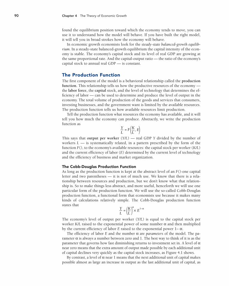
The efficiency of labor E and the number α are parameters of the model. The pa-rameter α is always a number between zero and 1. The best way to think of it is as theparameter that governs how fast diminishing returns to investment set in. A level of αnear zero means that the extra amount of output made possible by each additional unitof capital declines very quickly as the capital stock increases, as Figure 4.1 shows.

By contrast, a level of α near 1 means that the next additional unit of capital makespossible almost as large an increase in output as the last additional unit of capital, as

YL

KL

= ( E)α× 1–α

YL

KL

= F , E)(


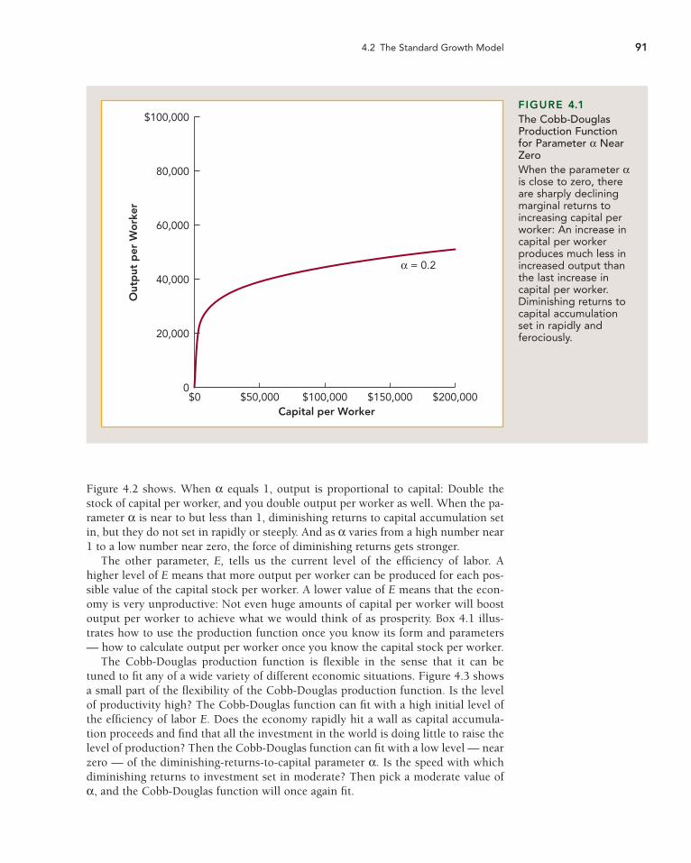
Figure 4.2 shows. When α equals 1, output is proportional to capital: Double thestock of capital per worker, and you double output per worker as well. When the pa-rameter α is near to but less than 1, diminishing returns to capital accumulation setin, but they do not set in rapidly or steeply. And as α varies from a high number near1 to a low number near zero, the force of diminishing returns gets stronger.

The other parameter, E, tells us the current level of the efficiency of labor. Ahigher level of E means that more output per worker can be produced for each pos-sible value of the capital stock per worker. A lower value of E means that the econ-omy is very unproductive: Not even huge amounts of capital per worker will boostoutput per worker to achieve what we would think of as prosperity. Box 4.1 illus-trates how to use the production function once you know its form and parameters— how to calculate output per worker once you know the capital stock per worker.

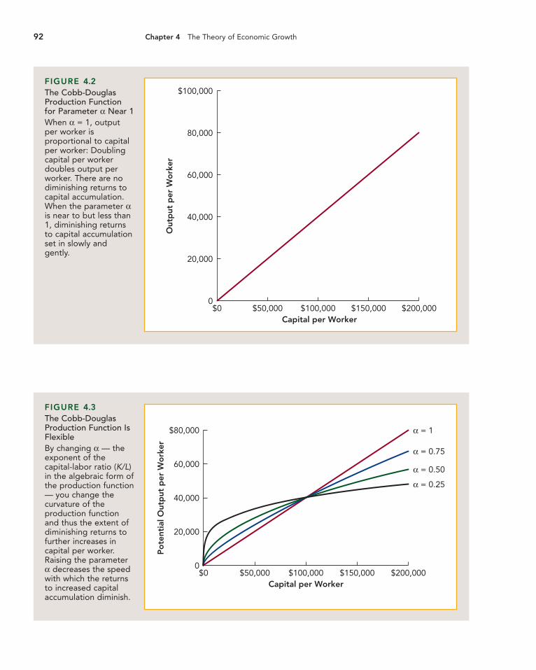
The Cobb-Douglas production function is flexible in the sense that it can betuned to fit any of a wide variety of different economic situations. Figure 4.3 showsa small part of the flexibility of the Cobb-Douglas production function. Is the levelof productivity high? The Cobb-Douglas function can fit with a high initial level ofthe efficiency of labor E. Does the economy rapidly hit a wall as capital accumula-tion proceeds and find that all the investment in the world is doing little to raise thelevel of production? Then the Cobb-Douglas function can fit with a low level — nearzero — of the diminishing-returns-to-capital parameter α. Is the speed with whichdiminishing returns to investment set in moderate? Then pick a moderate value ofα, and the Cobb-Douglas function will once again fit.


Out

put

per

Wo

rker

$100,000

80,000

60,000

40,000

20,000

0

Capital per Worker$0 $50,000 $100,000 $150,000 $200,000

α = 0.2

FIGURE 4.1The Cobb-DouglasProduction Functionfor Parameter α NearZeroWhen the parameter αis close to zero, thereare sharply decliningmarginal returns toincreasing capital perworker: An increase incapital per workerproduces much less inincreased output thanthe last increase incapital per worker.Diminishing returns tocapital accumulationset in rapidly andferociously.


Out

put

per

Wo

rker

$100,000

80,000

60,000

40,000

20,000

0


FIGURE 4.2The Cobb-DouglasProduction Functionfor Parameter α Near 1When α = 1, outputper worker isproportional to capitalper worker: Doublingcapital per workerdoubles output perworker. There are nodiminishing returns tocapital accumulation.When the parameter αis near to but less than1, diminishing returnsto capital accumulationset in slowly andgently.

Po

tent

ial O

utp

ut p

er W

ork

er

$80,000

60,000

40,000

20,000

0


α = 1

α = 0.75

α = 0.50

α = 0.25

FIGURE 4.3The Cobb-DouglasProduction Function IsFlexibleBy changing α — theexponent of thecapital-labor ratio (K/L)in the algebraic form ofthe production function— you change thecurvature of theproduction functionand thus the extent ofdiminishing returns tofurther increases incapital per worker.Raising the parameterα decreases the speedwith which the returnsto increased capitalaccumulation diminish.

No economist believes that there is, buried somewhere in the earth, a big machinethat forces the level of output per worker to behave exactly as calculated by the algebraic production function above. Instead, economists think that the Cobb-Douglas production function is a simple and useful approximation. The process thatdoes determine the level of output per worker is an immensely complex one: Every-one in the economy is part of it, and it is too complicated to work with. Using theCobb-Douglas production function involves a large leap of abstraction. Yet it is auseful leap, for using this approximation to analyze the economy will lead us to ap-proximately correct conclusions.

The Rest of the Growth ModelThe rest of the growth model is straightforward. First comes the need to keep trackof the quantities of the model over time. We do so by attaching to each variable —such as the capital stock, efficiency of labor, output per worker, or labor force — a


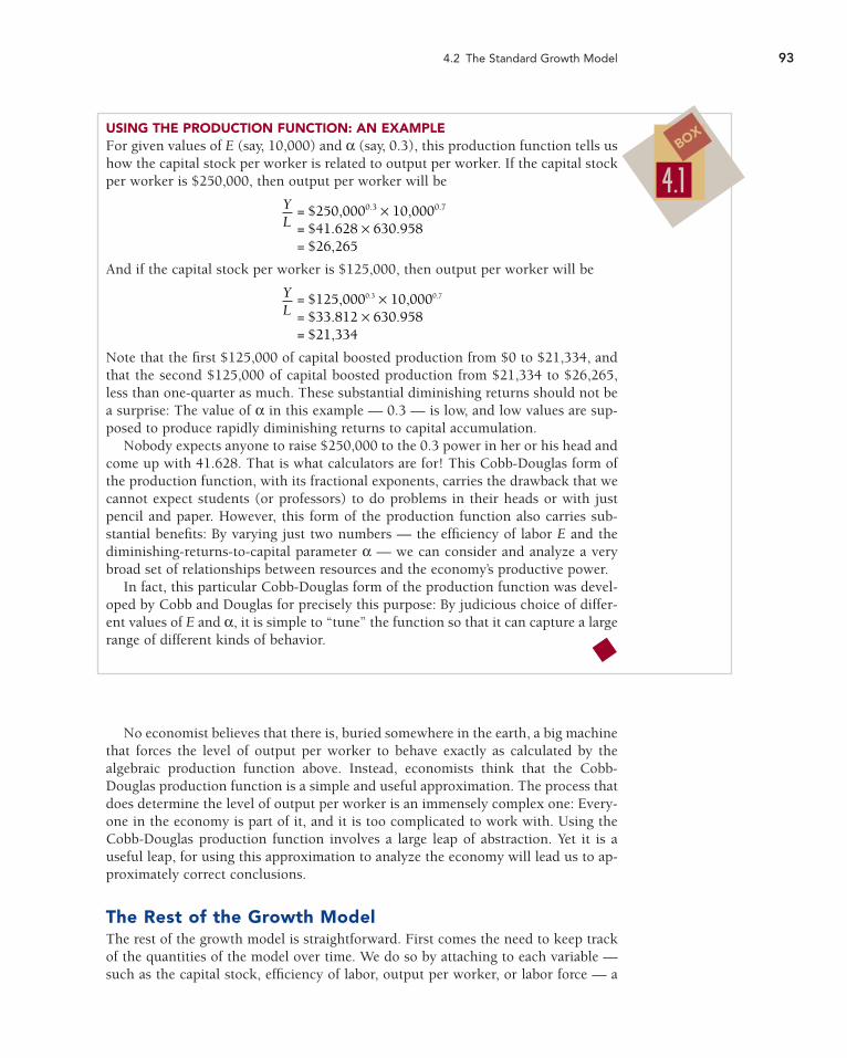
USING THE PRODUCTION FUNCTION: AN EXAMPLEFor given values of E (say, 10,000) and α (say, 0.3), this production function tells ushow the capital stock per worker is related to output per worker. If the capital stockper worker is $250,000, then output per worker will be

And if the capital stock per worker is $125,000, then output per worker will be

Note that the first $125,000 of capital boosted production from $0 to $21,334, andthat the second $125,000 of capital boosted production from $21,334 to $26,265,less than one-quarter as much. These substantial diminishing returns should not bea surprise: The value of α in this example — 0.3 — is low, and low values are sup-posed to produce rapidly diminishing returns to capital accumulation.

Nobody expects anyone to raise $250,000 to the 0.3 power in her or his head andcome up with 41.628. That is what calculators are for! This Cobb-Douglas form ofthe production function, with its fractional exponents, carries the drawback that wecannot expect students (or professors) to do problems in their heads or with justpencil and paper. However, this form of the production function also carries sub-stantial benefits: By varying just two numbers — the efficiency of labor E and the diminishing-returns-to-capital parameter α — we can consider and analyze a verybroad set of relationships between resources and the economy’s productive power.

In fact, this particular Cobb-Douglas form of the production function was devel-oped by Cobb and Douglas for precisely this purpose: By judicious choice of differ-ent values of E and α, it is simple to “tune” the function so that it can capture a largerange of different kinds of behavior.

YL

= $125,0000.3 × 10,0000.7

= $33.812 × 630.958= $21,334

YL

= $250,0000.3 × 10,0000.7

= $41.628 × 630.958= $26,265

4.1BOX

subscript telling what year it applies to. Thus K1999 will be the capital stock in year1999. If we want to refer to the efficiency of labor in the current year (but don’t carewhat the current year is), we use t (for “time”) as a stand-in for the numerical valueof the current year. Thus we write Et. And if we want to refer to the efficiency of laborin the year after the current year, we write Et+1.

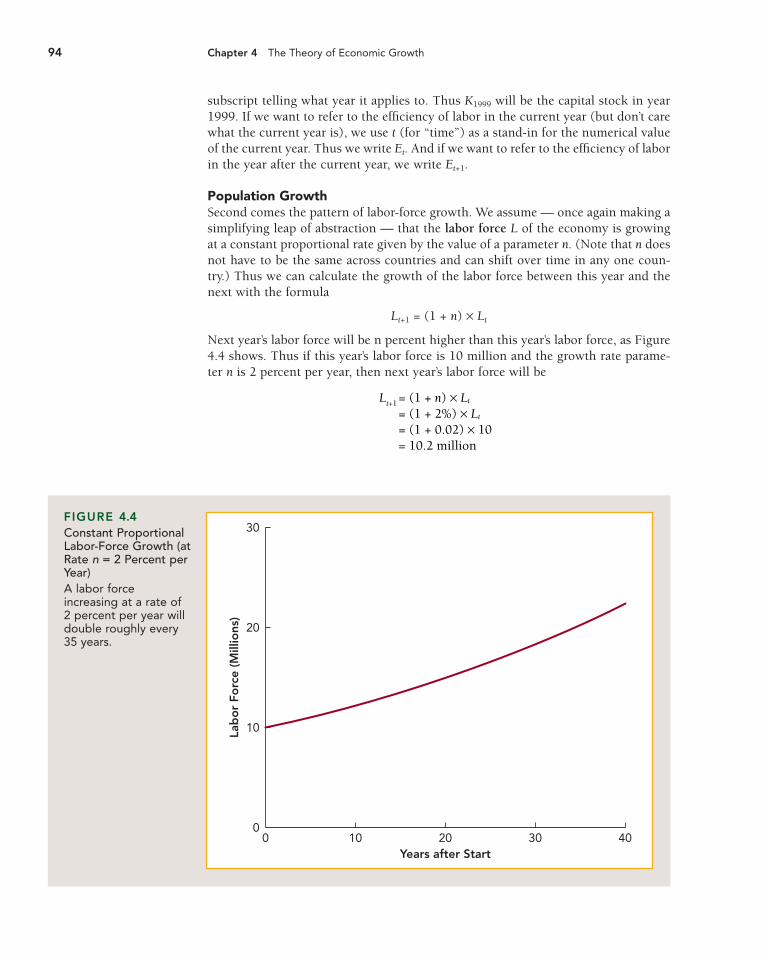
Population GrowthSecond comes the pattern of labor-force growth. We assume — once again making asimplifying leap of abstraction — that the labor force L of the economy is growingat a constant proportional rate given by the value of a parameter n. (Note that n doesnot have to be the same across countries and can shift over time in any one coun-try.) Thus we can calculate the growth of the labor force between this year and thenext with the formula

Lt+1 = (1 + n) × Lt

Next year’s labor force will be n percent higher than this year’s labor force, as Figure4.4 shows. Thus if this year’s labor force is 10 million and the growth rate parame-ter n is 2 percent per year, then next year’s labor force will be

Lt+1 = (1 + n) × Lt

= (1 + 2%) × Lt

= (1 + 0.02) × 10= 10.2 million


Lab

or

Forc

e (M

illio

ns)

30

20

10

0

Years after Start0 10 20 30 40

FIGURE 4.4Constant ProportionalLabor-Force Growth (atRate n = 2 Percent perYear) A labor forceincreasing at a rate of2 percent per year willdouble roughly every35 years.

We assume that the rate of growth of the labor force is constant not because webelieve that labor-force growth is unchanging but because the assumption makes theanalysis of the model simpler. The trade-off between realism in the model’s descrip-tion of the world and simplicity as a way to make the model easier to analyze is onethat economists always face. They usually resolve it in favor of simplicity.

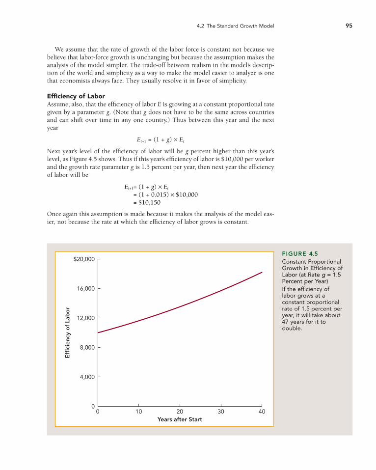
Efficiency of LaborAssume, also, that the efficiency of labor E is growing at a constant proportional rategiven by a parameter g. (Note that g does not have to be the same across countriesand can shift over time in any one country.) Thus between this year and the nextyear

Et+1 = (1 + g) × Et

Next year’s level of the efficiency of labor will be g percent higher than this year’slevel, as Figure 4.5 shows. Thus if this year’s efficiency of labor is $10,000 per workerand the growth rate parameter g is 1.5 percent per year, then next year the efficiencyof labor will be

Once again this assumption is made because it makes the analysis of the model eas-ier, not because the rate at which the efficiency of labor grows is constant.

Et+1= (1 + g) × Et

= (1 + 0.015) × $10,000= $10,150


Eff

icie

ncy

of

Lab

or

$20,000

16,000

12,000

8,000

4,000

0


FIGURE 4.5Constant ProportionalGrowth in Efficiency ofLabor (at Rate g = 1.5Percent per Year)If the efficiency oflabor grows at aconstant proportionalrate of 1.5 percent peryear, it will take about47 years for it todouble.

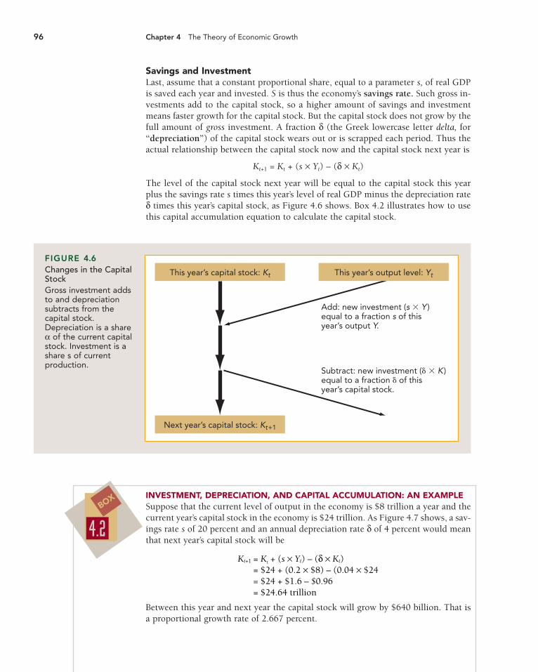
Savings and InvestmentLast, assume that a constant proportional share, equal to a parameter s, of real GDPis saved each year and invested. S is thus the economy’s savings rate. Such gross in-vestments add to the capital stock, so a higher amount of savings and investmentmeans faster growth for the capital stock. But the capital stock does not grow by thefull amount of gross investment. A fraction δ (the Greek lowercase letter delta, for“depreciation”) of the capital stock wears out or is scrapped each period. Thus theactual relationship between the capital stock now and the capital stock next year is

Kt+1 = Kt + (s × Yt) – (δ × Kt)

The level of the capital stock next year will be equal to the capital stock this yearplus the savings rate s times this year’s level of real GDP minus the depreciation rateδ times this year’s capital stock, as Figure 4.6 shows. Box 4.2 illustrates how to usethis capital accumulation equation to calculate the capital stock.


This year’s capital stock: Kt

Next year’s capital stock: Kt+1

This year’s output level: Yt

Add: new investment (s � Y)equal to a fraction s of this year’s output Y.

Subtract: new investment (� � K)equal to a fraction � of this year’s capital stock.

FIGURE 4.6Changes in the CapitalStockGross investment addsto and depreciationsubtracts from thecapital stock.Depreciation is a shareα of the current capitalstock. Investment is ashare s of currentproduction.

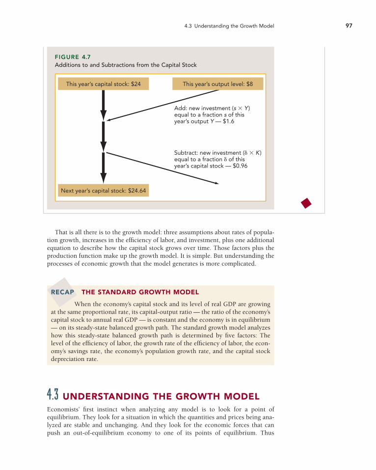
INVESTMENT, DEPRECIATION, AND CAPITAL ACCUMULATION: AN EXAMPLESuppose that the current level of output in the economy is $8 trillion a year and thecurrent year’s capital stock in the economy is $24 trillion. As Figure 4.7 shows, a sav-ings rate s of 20 percent and an annual depreciation rate δ of 4 percent would meanthat next year’s capital stock will be

Between this year and next year the capital stock will grow by $640 billion. That isa proportional growth rate of 2.667 percent.

Kt+1 = Kt + (s × Yt) – (δ × Kt)= $24 + (0.2 × $8) – (0.04 × $24= $24 + $1.6 – $0.96= $24.64 trillion

4.2BOX

That is all there is to the growth model: three assumptions about rates of popula-tion growth, increases in the efficiency of labor, and investment, plus one additionalequation to describe how the capital stock grows over time. Those factors plus theproduction function make up the growth model. It is simple. But understanding theprocesses of economic growth that the model generates is more complicated.

4.3 Understanding the Growth Model 97

This year’s capital stock: $24

Next year’s capital stock: $24.64

This year’s output level: $8

Add: new investment (s � Y)equal to a fraction s of this year’s output Y — $1.6

Subtract: new investment (� � K)equal to a fraction � of this year’s capital stock — $0.96

FIGURE 4.7Additions to and Subtractions from the Capital Stock

RECAP THE STANDARD GROWTH MODEL

When the economy’s capital stock and its level of real GDP are growingat the same proportional rate, its capital-output ratio — the ratio of the economy’scapital stock to annual real GDP — is constant and the economy is in equilibrium— on its steady-state balanced growth path. The standard growth model analyzeshow this steady-state balanced growth path is determined by five factors: Thelevel of the efficiency of labor, the growth rate of the efficiency of labor, the econ-omy’s savings rate, the economy’s population growth rate, and the capital stockdepreciation rate.

4.3 UNDERSTANDING THE GROWTH MODELEconomists’ first instinct when analyzing any model is to look for a point of equilibrium. They look for a situation in which the quantities and prices being ana-lyzed are stable and unchanging. And they look for the economic forces that canpush an out-of-equilibrium economy to one of its points of equilibrium. Thus

microeconomists talk about the equilibrium of a particular market. Macroecono-mists talk (as we will later in the book) about the equilibrium value of real GDP rel-ative to potential output.

In the study of long-run growth, however, the key economic quantities are neverstable. They are growing over time. The efficiency of labor is growing; the level ofoutput per worker is growing; the capital stock is growing; the labor force is grow-ing. How, then, can we talk about a point of equilibrium where things are stable ifeverything is growing?

The answer is to look for an equilibrium in which everything is growing together,at the same proportional rate. Such an equilibrium is one of steady-state balancedgrowth. If everything is growing together, then the relationships between key quan-tities in the economy are stable. And the material in this chapter will be easier if wefocus on one key ratio: the capital-output ratio. Thus our point of equilibrium willbe one at which the capital-output ratio is constant over time and toward which thecapital-output ratio will converge if it should find itself out of equilibrium.

How Fast Is the Economy Growing?We know that the key quantities in the economy are growing. The efficiency of labor is, after all, increasing at a proportional rate g. And we know that it is technology-driven improvements in the efficiency of labor that have generated mostof the increases in our material welfare and economic productivity over the past fewcenturies.

Determining how fast the quantities in the economy are growing is straightfor-ward if we remember our three mathematical rules:

• The proportional growth rate of a product — P × Q, say — is equal to the sumof the proportional growth rates of the factors, that is, the growth rate of P plusthe growth rate of Q.

• The proportional growth rate of a quotient — E/Q, say — is equal to thedifference of the proportional growth rates of the dividend (E) and the divisor(Q).

• The proportional growth rate of a quantity raised to a exponent — Qy, say — isequal to the exponent (y) times the growth rate of the quantity (Q).

The Growth of Capital per WorkerBegin with capital per worker. To reduce the length of equations, let’s use the ex-pression g(kt) to stand for the proportional growth rate of capital per worker. Theproportional growth rate is simply the amount that output per worker will be nextyear minus the amount it is this year, all divided by the output per worker this year:

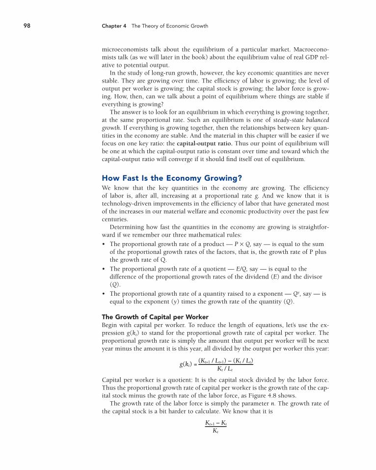
Capital per worker is a quotient: It is the capital stock divided by the labor force.Thus the proportional growth rate of capital per worker is the growth rate of the cap-ital stock minus the growth rate of the labor force, as Figure 4.8 shows.

The growth rate of the labor force is simply the parameter n. The growth rate ofthe capital stock is a bit harder to calculate. We know that it is

Kt

Kt+1 – Kt

g(kt) = Kt / Lt

(Kt+1 / Lt+1) – (Kt / Lt)


And we know that we can write next year’s capital stock as equal to this year’s capi-tal stock plus gross investment minus depreciation:

Kt+1 = Kt + (s × Yt) – (δ × Kt)

If we substitute in for next year’s capital stock and rearrange, we have

Then we see that the proportional growth rate of capital per worker is

To make our equations look simpler, let’s give the capital-output ratio K/Y a specialsymbol: κ (the Greek letter kappa). Thus we can write that the proportional growthrate of capital per worker is

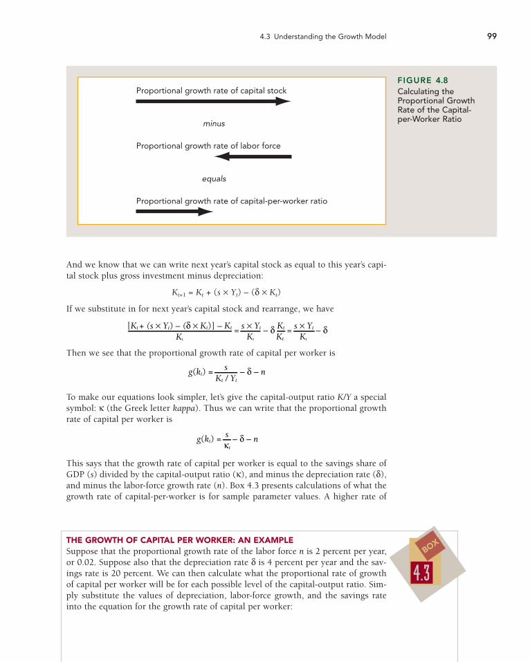
This says that the growth rate of capital per worker is equal to the savings share ofGDP (s) divided by the capital-output ratio (κ), and minus the depreciation rate (δ),and minus the labor-force growth rate (n). Box 4.3 presents calculations of what thegrowth rate of capital-per-worker is for sample parameter values. A higher rate of

g(kt) = κt

s – δ – n

g(kt) = Kt / Yt

s – δ – n

Kt

[Kt + (s × Yt) – (δ × Kt)] – Kt = s × Yt – δ Kt = s × Yt – δKt Kt Kt


Proportional growth rate of capital stock

minus

equals

Proportional growth rate of capital-per-worker ratio

Proportional growth rate of labor force

FIGURE 4.8Calculating theProportional GrowthRate of the Capital-per-Worker Ratio

THE GROWTH OF CAPITAL PER WORKER: AN EXAMPLESuppose that the proportional growth rate of the labor force n is 2 percent per year,or 0.02. Suppose also that the depreciation rate δ is 4 percent per year and the sav-ings rate is 20 percent. We can then calculate what the proportional rate of growthof capital per worker will be for each possible level of the capital-output ratio. Sim-ply substitute the values of depreciation, labor-force growth, and the savings rateinto the equation for the growth rate of capital per worker:

4.3BOX

to get

Then if the current capital-output ratio is 5, the growth rate of capital per workerwill be

At minus 2 percent per year, the capital-per-worker ratio is shrinking. By contrast, ifthe current capital-output ratio is 2.5, the growth rate of capital per worker will be

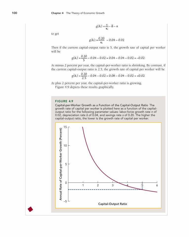
At plus 2 percent per year, the capital-per-worker ratio is growing.Figure 4.9 depicts these results graphically.

g(kt) = 2.5

0.20 – 0.04 – 0.02 = 0.08 – 0.04 – 0.02 = +0.02

g(kt) = 5

0.20 – 0.04 – 0.02 = 0.04 – 0.04 – 0.02 = –0.02

g(kt) = κt

0.20 – 0.04 – 0.02

g(kt) = κt

s – δ – n

Ann

ual R

ate

of

Cap

ital

-per

-Wo

rker

Gro

wth

(P

erce

nt) 15

10

0

5

–5Capital-Output Ratio

1 2 3 4 65

FIGURE 4.9Capital-per-Worker Growth as a Function of the Capital-Output Ratio Thegrowth rate of capital per worker is plotted here as a function of the capital-output ratio for the following parameter values: labor-force growth rate n of0.02, depreciation rate δ of 0.04, and savings rate s of 0.20. The higher thecapital-output ratio, the lower is the growth rate of capital per worker.


labor-force growth will reduce the rate of growth of capital per worker: Having moreworkers means the available capital has to be divided up more ways. A higher rateof depreciation will reduce the rate of growth of capital per worker: More capital willrust away. And a higher capital-output ratio will reduce the proportional growth rateof capital per worker: The higher the capital-output ratio, the smaller is investmentrelative to the capital stock.

The Growth of Output per WorkerOur Cobb-Douglas form of the production function tells us that the level of outputper worker is

Output per worker is the product of two terms, each of which is a quantity raised toa exponential power. So using our mathematical rules of thumb, the proportionalgrowth rate of output per worker — call it g(yt) to once again save space — will be,as Figure 4.10 shows

• α times the proportional growth rate of capital per worker.

• Plus (1 – α) times the rate of growth of the efficiency of labor.

The rate of growth of the efficiency of labor is simply g. And the previous sectioncalculated the growth rate of capital per worker g(k): s/κt – δ – n. So simply plugthese expressions in

And simplify a bit by rearranging terms:

g(yt) = g + α × κt

s – (n + g + δ)[ ]}{

g(yt) = α × κt

s – δ – n + [(1 – α) × g]( )[ ]

Yt

Lt

Kt

Lt

= ( Et)α× 1–α


Growth Rate of Efficiency of Labor: g

α times this: (1 minus α) times this:plus

equals

Growth Rate of Output per Worker: g(y)

Growth Rate of Capital per Worker: g(k)

FIGURE 4.10Calculating the Growth Rate of Output per Worker The growth rate of output per worker is a weighted average of the growth rates of capital per worker andefficiency of labor.

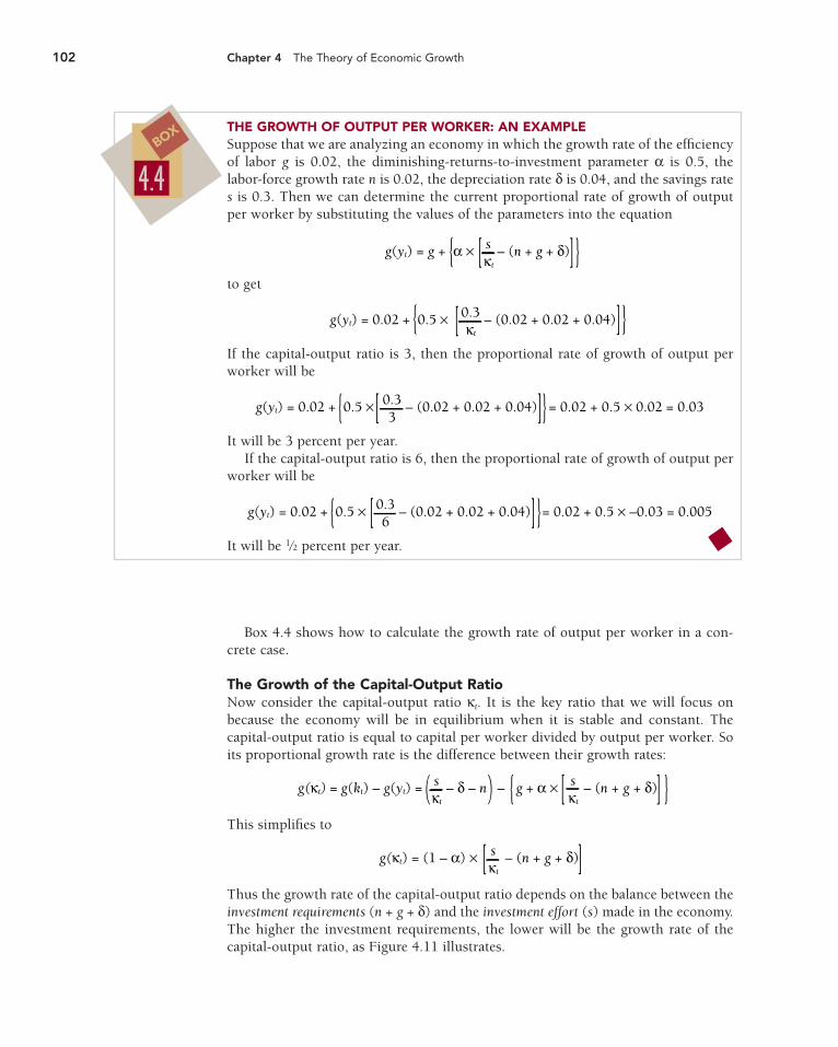
Box 4.4 shows how to calculate the growth rate of output per worker in a con-crete case.

The Growth of the Capital-Output RatioNow consider the capital-output ratio κt. It is the key ratio that we will focus on because the economy will be in equilibrium when it is stable and constant. The capital-output ratio is equal to capital per worker divided by output per worker. Soits proportional growth rate is the difference between their growth rates:

This simplifies to

Thus the growth rate of the capital-output ratio depends on the balance between theinvestment requirements (n + g + δ) and the investment effort (s) made in the economy.The higher the investment requirements, the lower will be the growth rate of thecapital-output ratio, as Figure 4.11 illustrates.

g(κt) = (1 – α) × κt

s[ – (n + g + δ)]

g(κt) = g(kt) – g(yt) = κt

s – δ – n( ) – g + α ×κt

s[ – (n + g + δ) ]{ }


THE GROWTH OF OUTPUT PER WORKER: AN EXAMPLESuppose that we are analyzing an economy in which the growth rate of the efficiencyof labor g is 0.02, the diminishing-returns-to-investment parameter α is 0.5, thelabor-force growth rate n is 0.02, the depreciation rate δ is 0.04, and the savings rates is 0.3. Then we can determine the current proportional rate of growth of outputper worker by substituting the values of the parameters into the equation

to get

If the capital-output ratio is 3, then the proportional rate of growth of output perworker will be

It will be 3 percent per year.If the capital-output ratio is 6, then the proportional rate of growth of output per

worker will be

It will be 1⁄2 percent per year.

g(yt) = 0.02 + 0.5 × 6

0.3 – (0.02 + 0.02 + 0.04) = 0.02 + 0.5 × –0.03 = 0.005[ ]}{

g(yt) = 0.02 + 0.5 × 3

0.3 – (0.02 + 0.02 + 0.04) = 0.02 + 0.5 × 0.02 = 0.03[ ]{ }

g(yt) = 0.02 + 0.5 × κt

0.3 – (0.02 + 0.02 + 0.04)[ ]}{

g(yt) = g + α × κt

s – (n + g + δ)[ ]}{

4.4BOX

Steady-State Growth Equilibrium

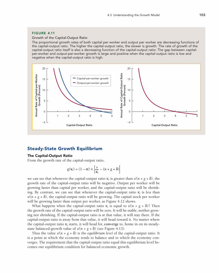
The Capital-Output RatioFrom the growth rate of the capital-output ratio,

we can see that whenever the capital-output ratio κt is greater than s/(n + g + δ), thegrowth rate of the capital-output ratio will be negative. Output per worker will begrowing faster than capital per worker, and the capital-output ratio will be shrink-ing. By contrast, we can see that whenever the capital-output ratio κt is less than s/(n + g + δ), the capital-output ratio will be growing. The capital stock per workerwill be growing faster than output per worker, as Figure 4.12 shows.

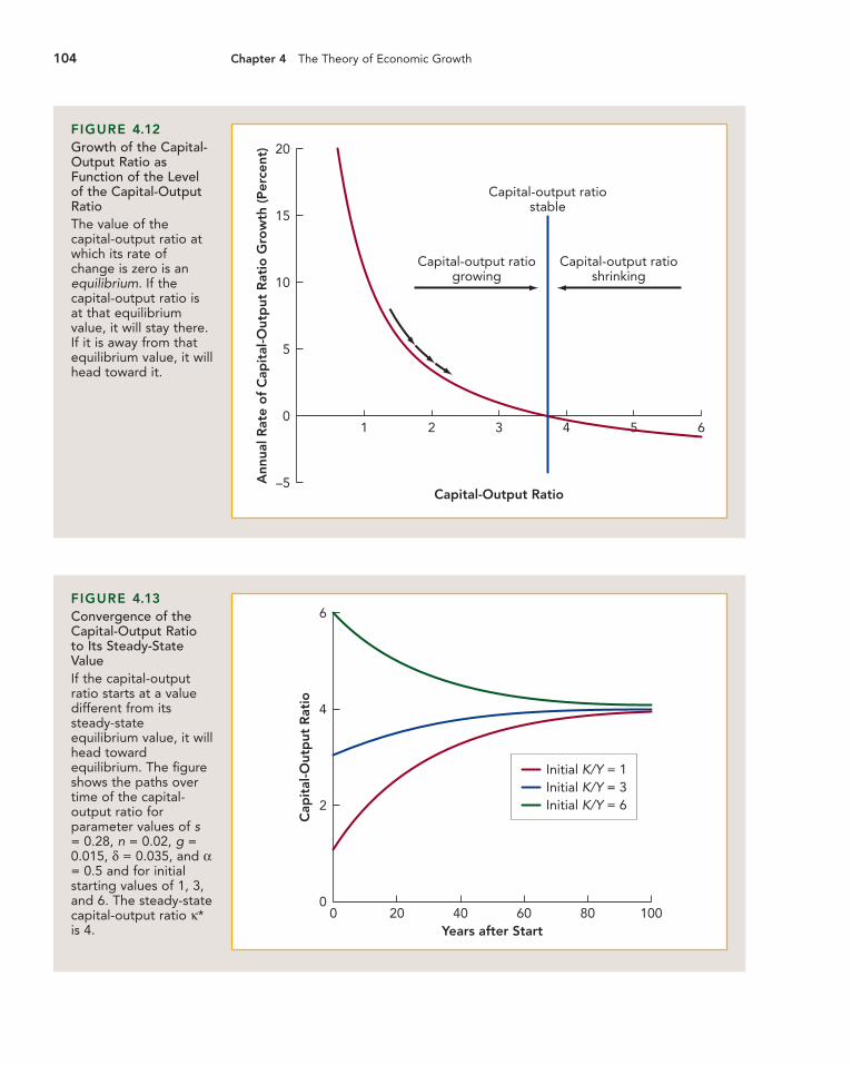
What happens when the capital-output ratio κt is equal to s/(n + g + δ)? Then the growth rate of the capital-output ratio will be zero. It will be stable, neither grow-ing nor shrinking. If the capital-output ratio is at that value, it will stay there. If thecapital-output ratio is away from that value, it will head toward it. No matter wherethe capital-output ratio κt starts, it will head for, converge to, home in on its steady-state balanced-growth value of s/(n + g + δ) (see Figure 4.13).

Thus the value s/(n + g + δ) is the equilibrium level of the capital-output ratio. Itis a point at which the economy tends to balance and to which the economy con-verges. The requirement that the capital-output ratio equal this equilibrium level be-comes our equilibrium condition for balanced economic growth.

g(κt) = (1 – α) × κt

s[ – (n + g + δ)]


Ann

ual R

ate

of

Cap

ital

-Out

out

Rat

ioG

row

th (P

erce

nt)

20

15

10

0

5


1 2 3 4 65Ann

ual R

ate

of

Cap

ital

-per

-Wo

rker

Gro

wth

(P

erce

nt)

20

15

10

0

5


1 2 3 4 65

Capital-per-worker growth

Output-per-worker growth

FIGURE 4.11Growth of the Capital-Output RatioThe proportional growth rates of both capital per worker and output per worker are decreasing functions ofthe capital-output ratio. The higher the capital-output ratio, the slower is growth. The rate of growth of thecapital-output ratio itself is also a decreasing function of the capital-output ratio: The gap between capital-per-worker and output-per-worker growth is large and positive when the capital-output ratio is low andnegative when the capital-output ratio is high.


Ann

ual R

ate

of

Cap

ital

-Out

put

Rat

io G

row

th (

Per

cent

) 20

15

10

0

5


1 2 3 4

Capital-output ratiostable

Capital-output ratioshrinking

65

Capital-output ratiogrowing

FIGURE 4.12Growth of the Capital-Output Ratio asFunction of the Levelof the Capital-OutputRatioThe value of thecapital-output ratio atwhich its rate ofchange is zero is anequilibrium. If thecapital-output ratio isat that equilibriumvalue, it will stay there.If it is away from thatequilibrium value, it willhead toward it.

Cap

ital

-Out

put

Rat

io

6

4

2

0


Initial K/Y = 1Initial K/Y = 3Initial K/Y = 6

FIGURE 4.13Convergence of theCapital-Output Ratioto Its Steady-StateValueIf the capital-outputratio starts at a valuedifferent from itssteady-stateequilibrium value, it willhead towardequilibrium. The figureshows the paths overtime of the capital-output ratio forparameter values of s= 0.28, n = 0.02, g =0.015, δ = 0.035, and α= 0.5 and for initialstarting values of 1, 3,and 6. The steady-statecapital-output ratio κ*is 4.

To make our future equations even simpler, we can give the quantity s/(n + g+ δ)— the equilibrium value of the capital-output ratio — the symbol κ*:

Other QuantitiesWhen the capital-output ratio κt is at its steady-state value of

the proportional growth rates of capital per worker and output per worker are sta-ble too. Output per worker is growing at a proportional rate g:

g(yt) = g

The capital stock per worker is growing at the same proportional rate g:

g(kt) = g

The total economywide capital stock is then growing at the proportional rate n + g:the growth rate of capital per worker plus the growth rate of the labor force. RealGDP is also growing at rate n + g: the growth rate of output per worker plus the laborforce growth rate.

The Level of Output per Worker on the Steady-State Growth PathWhen the capital-output ratio is at its steady-state balanced-growth equilibriumvalue κ*, we say that the economy is on its steady-state growth path. What is thelevel of output per worker if the economy is on this path? We saw the answer to thisin Chapter 3. The requirement that the economy be on its steady-state growth pathwas then our equilibrium condition:

In order to combine it with the production function,

we first rewrote the production function to make capital per worker the product ofthe capital-output ratio and output per worker:

Dividing both sides by (Y/L)α,

and then raising both sides to the 1/(1 – α) power produce an equation for the levelof output per worker:

Yt

Lt

Kt

Yt

= Et

α×1–α( )

Yt

Lt

Kt

Yt

=( Et)α 1–α×

1–α ( )

Yt

Lt

Kt

Yt

= ( Et)α× 1–αYt

Lt×

Yt

Lt

Kt

Lt

= ( Et)α× 1–α

κ* = sn + g + δYt

Kt =

κ* = sn + g + δ

κ* = sn + g + δ


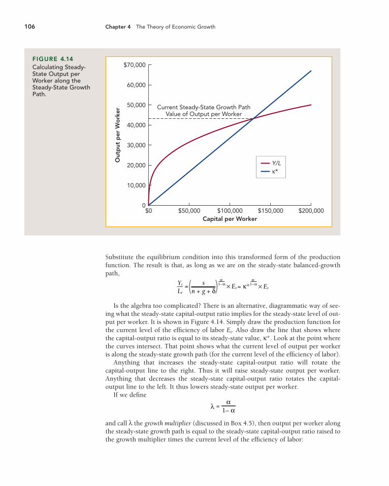
Substitute the equilibrium condition into this transformed form of the productionfunction. The result is that, as long as we are on the steady-state balanced-growthpath,

Is the algebra too complicated? There is an alternative, diagrammatic way of see-ing what the steady-state capital-output ratio implies for the steady-state level of out-put per worker. It is shown in Figure 4.14. Simply draw the production function forthe current level of the efficiency of labor Et. Also draw the line that shows wherethe capital-output ratio is equal to its steady-state value, κ*. Look at the point wherethe curves intersect. That point shows what the current level of output per workeris along the steady-state growth path (for the current level of the efficiency of labor).

Anything that increases the steady-state capital-output ratio will rotate the capital-output line to the right. Thus it will raise steady-state output per worker.Anything that decreases the steady-state capital-output ratio rotates the capital-output line to the left. It thus lowers steady-state output per worker.

If we define

and call λ the growth multiplier (discussed in Box 4.5), then output per worker alongthe steady-state growth path is equal to the steady-state capital-output ratio raised tothe growth multiplier times the current level of the efficiency of labor:

=α

1– αλ

Yt

Lt

= Et = κ*α

×1–α( )sn + g + δ

α1–α Et×


Out

put

per

Wo

rker

$70,000

60,000

50,000

40,000

20,000

30,000

10,000

0


Current Steady-State Growth PathValue of Output per Worker

Y/Lκ*

FIGURE 4.14Calculating Steady-State Output perWorker along theSteady-State GrowthPath.

Thus calculating output per worker when the economy is on its steady-state growthpath is a simple three-step procedure:

1. Calculate the steady-state capital-output ratio, κ* = s/(n + g + δ), the savingsrate divided by the sum of the population growth rate, the efficiency of laborgrowth rate, and the depreciation rate.

2. Amplify the steady-state capital-output ratio κ* by the growth multiplier. Raiseit to the λ = α/(1 – α) power, where α is the diminishing-returns-to-capitalparameter.

3. Multiply the result by the current value of the efficiency of labor Et, which canbe easily calculated because the efficiency of labor is growing at the constantproportional rate g.

The fact that an economy converges to its steady-state growth path makes ana-lyzing the long-run growth of an economy relatively easy as well:

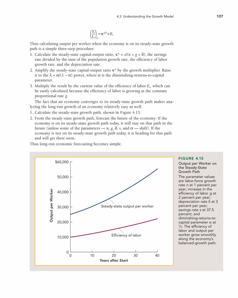
1. Calculate the steady-state growth path, shown in Figure 4.15.

2. From the steady-state growth path, forecast the future of the economy: If theeconomy is on its steady-state growth path today, it will stay on that path in thefuture (unless some of the parameters — n, g, δ, s, and α — shift). If theeconomy is not on its steady-state growth path today, it is heading for that pathand will get there soon.

Thus long-run economic forecasting becomes simple.

Yt

Lt

=( Et) ×ss

κ*λ


Out

put

per

Wo

rker

$60,000

50,000

40,000

30,000

20,000

10,000

0


Efficiency of labor

Steady-state output per worker

FIGURE 4.15Output per Worker onthe Steady-StateGrowth PathThe parameter valuesare labor-force growthrate n at 1 percent peryear; increase in theefficiency of labor g at2 percent per year;depreciation rate δ at 3percent per year;savings rate s at 37.5percent; anddiminishing-returns-to-capital parameter α at1⁄3. The efficiency oflabor and output perworker grow smoothlyalong the economy’sbalanced-growth path.


WHERE THE GROWTH MULTIPLIER COMES FROM: THE DETAILSWhy is the steady-state capital-output ratio raised to the (larger) power of α/(1 – α)rather than just the power α? The power used makes a big difference when one ap-plies the growth model to different situations.

The reason is that an increase in the capital-output ratio increases the capitalstock both directly and indirectly. For the same level of output you have more capi-tal. And because extra output generated by the additional capital is itself a source ofadditional savings and investment, you have even more capital. The impact of theadditional capital generated by anything that raises κ* — an increase in savings, adecrease in labor force, or anything else — is thus multiplied by these positive feed-back effects.

Figure 4.16 shows the effect of this difference between α and α/(1 – α). An in-crease in the capital-output ratio means more capital for a given level of output, andthat generates the first-round increase in output: amplification by the increase incapital raised to the power α. But the first-round increase in output generates stillmore capital, which increases production further. The total increase in production isthe proportional increase in the steady-state capital-output ratio raised to the(larger) power α/(1 – α).

4.5BOX

Out

put

per

Wo

rker

$140,000

120,000 Total increase in SS output per worker

First-round increase inSS output per worker100,000

80,000

60,000

40,000

20,000

0

Capital per Worker0 $100,000 $200,000 $300,000 $400,000

Y/Lκ*κ* (new)

FIGURE 4.16The Growth Multiplier: Effect of Increasing Capital-Output Ratio on Steady-State (SS) Output per Worker

How Fast Does the Economy Head For Its Steady-State Growth Path?Suppose that the capital-output ratio κt is not at its steady-state value κ*? How fastdoes it approach its steady state? Even in this simple growth model we can’t get anexact answer. But if we are willing to settle for approximations and confine our attention only to small differences beween the current capital-output ratio κt and itssteady-state value κ*, then we can get an answer. The growth rate of the capital-output ratio will be approximately equal to a fraction [(1 – α) × (n + g + δ)] of thegap between the steady-state and its current level.

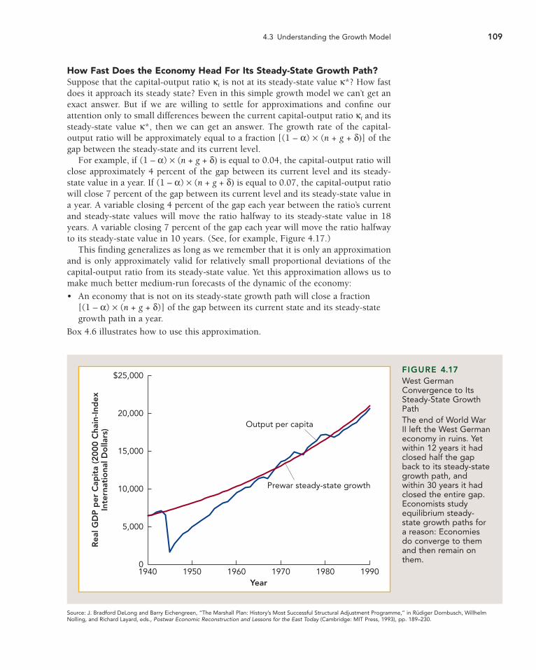
For example, if (1 – α) × (n + g + δ) is equal to 0.04, the capital-output ratio willclose approximately 4 percent of the gap between its current level and its steady-state value in a year. If (1 – α) × (n + g + δ) is equal to 0.07, the capital-output ratiowill close 7 percent of the gap between its current level and its steady-state value ina year. A variable closing 4 percent of the gap each year between the ratio’s currentand steady-state values will move the ratio halfway to its steady-state value in 18years. A variable closing 7 percent of the gap each year will move the ratio halfwayto its steady-state value in 10 years. (See, for example, Figure 4.17.)

This finding generalizes as long as we remember that it is only an approximationand is only approximately valid for relatively small proportional deviations of thecapital-output ratio from its steady-state value. Yet this approximation allows us tomake much better medium-run forecasts of the dynamic of the economy:

• An economy that is not on its steady-state growth path will close a fraction [(1 – α) × (n + g + δ)] of the gap between its current state and its steady-stategrowth path in a year.

Box 4.6 illustrates how to use this approximation.


Rea

l GD

P p

er C

apit

a (2

00

0 C

hain

-Ind

exIn

tern

atio

nal D

olla

rs)

$25,000

20,000

15,000

10,000

5,000

0

Year1940 1950 1960 1970 19901980

Prewar steady-state growth

Output per capita

FIGURE 4.17West GermanConvergence to ItsSteady-State GrowthPath The end of World WarII left the West Germaneconomy in ruins. Yetwithin 12 years it hadclosed half the gapback to its steady-stategrowth path, andwithin 30 years it hadclosed the entire gap.Economists studyequilibrium steady-state growth paths fora reason: Economiesdo converge to themand then remain onthem.

Source: J. Bradford DeLong and Barry Eichengreen, “The Marshall Plan: History’s Most Successful Structural Adjustment Programme,” in Rüdiger Dornbusch, WillhelmNolling, and Richard Layard, eds., Postwar Economic Reconstruction and Lessons for the East Today (Cambridge: MIT Press, 1993), pp. 189–230.

Thus short- and medium-run forecasting becomes simple too. All you have to dois predict that the economy will head for its steady-state growth path and calculatewhat the steady-state growth path is.


CONVERGING TO THE STEADY-STATE BALANCED-GROWTH PATH: AN EXAMPLEConsider an economy with parameter values of population growth n = 0.02, effi-ciency of labor growth g = 0.015, depreciation δ = 0.035, and diminishing-returns-to-investment parameter δ = 0.5 — the economy whose capital-output ratio isshowed in Figure 4.11. This economy would, if off its steady-state growth path, closea fraction of the gap between its current state and its steady state each year:

This 3.5 percent rate of convergence would allow the economy to close half of thegap to the steady-state in 20 years.

(1 – α) × (n + g + δ) = (1 – 0.5) × (0.02 + 0.015 + 0.035) = 0.5 × 0.07 = 0.035

4.6BOX

Out

put

per

Wo

rker

(as

Per

cent

age

of

U.S

. Le

vel)

120

100

80

60

40

20

0

Labor-Force Growth (Percent)0 1 2 3 54

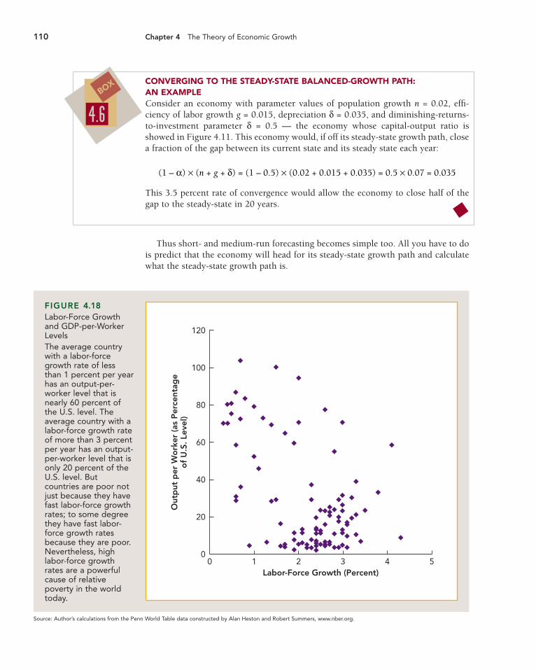
FIGURE 4.18Labor-Force Growthand GDP-per-WorkerLevels The average countrywith a labor-forcegrowth rate of lessthan 1 percent per yearhas an output-per-worker level that isnearly 60 percent ofthe U.S. level. Theaverage country with alabor-force growth rateof more than 3 percentper year has an output-per-worker level that isonly 20 percent of theU.S. level. Butcountries are poor notjust because they havefast labor-force growthrates; to some degreethey have fast labor-force growth ratesbecause they are poor.Nevertheless, highlabor-force growthrates are a powerfulcause of relativepoverty in the worldtoday.

Source: Author’s calculations from the Penn World Table data constructed by Alan Heston and Robert Summers, www.nber.org.

Determining the Steady-State Capital-Output Ratio

Labor-Force GrowthThe faster the growth rate of the labor force, the lower will be the economy’s steady-state capital-output ratio. Why? Because each new worker who joins the labor forcemust be equipped with enough capital to be productive and to, on average, matchthe productivity of his or her peers. The faster the rate of growth of the labor force,the larger the share of current investment that must go to equip new members of thelabor force with the capital they need to be productive. Thus the lower will be theamount of investment that can be devoted to building up the average ratio of capi-tal to output.

A sudden and permanent increase in the rate of growth of the labor force willlower the level of output per worker on the steady-state growth path. How large willthe long-run change in the level of output be, relative to what would have happenedhad population growth not increased? It is straightforward to calculate if we knowwhat the other parameter values of the economy are.

How important is all this in the real world? Does a high rate of labor-force growthplay a role in making countries relatively poor not just in economists’ models but inreality? It turns out that it is important, as Figure 4.18 shows. Of the 22 countries inthe world with GDP-per-worker levels at least half of the U.S. level, 18 have labor-force growth rates of less than 2 percent per year, and 12 have labor-force growth ratesof less than 1 percent per year. The additional investment requirements imposed byrapid labor-force growth are a powerful reducer of capital intensity and a powerful ob-stacle to rapid economic growth. Box 4.7 shows just how powerful these effects are.


AN INCREASE IN POPULATION GROWTH: AN EXAMPLEConsider an economy in which the parameter α is 1⁄2 — so the growth multiplier γ = α/(1 – α) is 1 — in which the underlying rate of productivity growth g is 1.5 per-cent per year, the depreciation rate δ is 3.5 percent per year, and the savings rate s is21 percent. Suppose that the labor-force growth rate suddenly and permanently in-creases from 1 to 2 percent per year.

Then before the increase in population growth the steady-state capital outputratio was

After the increase in population growth, the new steady-state capital-output ratiowill be

Before the increase in population growth, the level of output per worker along theold steady-state growth path was

After the increase in population growth, the level of output per worker along thenew steady-state growth path will be

Yt

Lt

= (( Et = 3.01 × Et ) ×ss,new

κ*)λ

Yt

Lt

= (( Et = 3.51 × Et ) ×ss,old

κ*)λ

newκ* = snnew + g + δ

.21.02 + .015 + .035

= .21.07

= = 3

oldκ* = snold + g + δ

.21.01 + .015 + .035

= .21.06

= = 3.5

4.7BOX

Divide the second of the equations by the first:

And discover that output per worker along the new steady-state growth path is only86 percent of what it would have been along the old steady-state growth path: Fasterpopulation growth means that output per worker along the steady-state growth pathhas fallen by 14 percent.

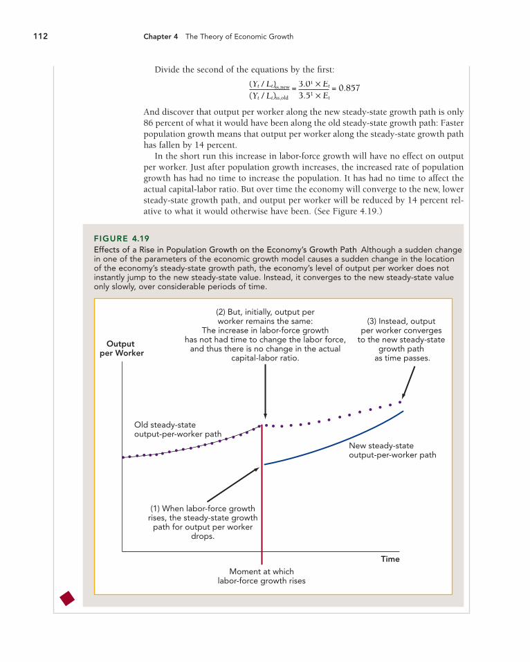
In the short run this increase in labor-force growth will have no effect on outputper worker. Just after population growth increases, the increased rate of populationgrowth has had no time to increase the population. It has had no time to affect theactual capital-labor ratio. But over time the economy will converge to the new, lowersteady-state growth path, and output per worker will be reduced by 14 percent rel-ative to what it would otherwise have been. (See Figure 4.19.)

(Yt / Lt)(Yt / Lt)

= 3.01 × Et

ss,old

ss,new

3.51 × Et = 0.857


Output per Worker

(1) When labor-force growthrises, the steady-state growth

path for output per workerdrops.

Moment at whichlabor-force growth rises

(3) Instead, output per worker converges

to the new steady-state growth path

as time passes.

New steady-stateoutput-per-worker path

Old steady-stateoutput-per-worker path

(2) But, initially, output perworker remains the same:

The increase in labor-force growthhas not had time to change the labor force,

and thus there is no change in the actualcapital-labor ratio.

Time

FIGURE 4.19Effects of a Rise in Population Growth on the Economy’s Growth Path Although a sudden changein one of the parameters of the economic growth model causes a sudden change in the locationof the economy’s steady-state growth path, the economy’s level of output per worker does notinstantly jump to the new steady-state value. Instead, it converges to the new steady-state valueonly slowly, over considerable periods of time.

Depreciation and Productivity GrowthIncreases or decreases in the depreciation rate will have the same effects on thesteady-state capital-output ratio and on output per worker along the steady-stategrowth path as will increases or decreases in the labor-force growth rate. The higherthe depreciation rate, the lower will be the economy’s steady-state capital-outputratio. Why? Because a higher depreciation rate means that the existing capital stockwears out and must be replaced more quickly. The higher the depreciation rate, thelarger the share of current investment that must go to replacing the capital that hasbecome worn out or obsolete. Thus the lower will be the amount of investment thatcan be devoted to building up the average ratio of capital to output.

Increases or decreases in the rate of productivity growth will have effects similarto those of increases or decreases in the labor-force growth rate on the steady-statecapital-output ratio, but they will have very different effects on the steady-state levelof output per worker. The faster the growth rate of productivity, the lower will be theeconomy’s steady-state capital-output ratio. The faster the productivity growth, thehigher is output now. But the capital stock depends on what investment was in the past. The faster the productivity growth, the smaller is past investment relativeto current production and the lower is the average ratio of capital to output. So achange in productivity growth will have the same effects on the steady-state capital-output ratio as will an equal change in labor-force growth.

But a change in productivity growth will have very different effects on output perworker along the steady-state growth path. Output per worker along the steady-stategrowth path is

While an increase in the productivity growth rate g lowers κ*, it increases the rateof growth of the efficiency of labor E, and so in the long run it does not lower butraises output per worker along the steady-state growth path.

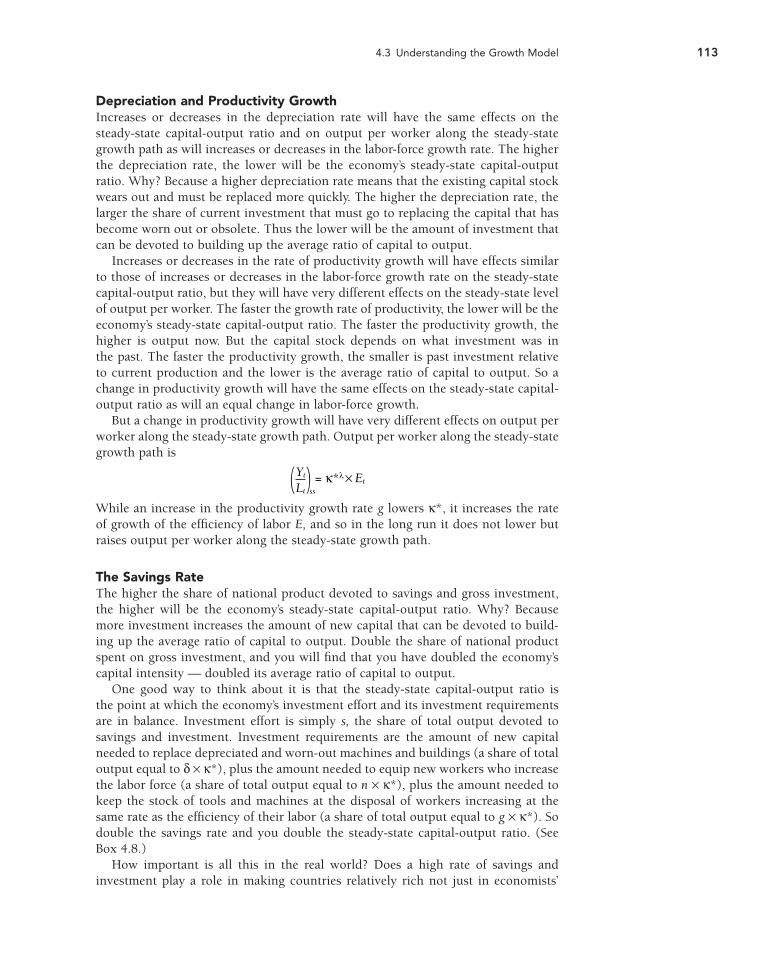
The Savings RateThe higher the share of national product devoted to savings and gross investment,the higher will be the economy’s steady-state capital-output ratio. Why? Becausemore investment increases the amount of new capital that can be devoted to build-ing up the average ratio of capital to output. Double the share of national productspent on gross investment, and you will find that you have doubled the economy’scapital intensity — doubled its average ratio of capital to output.

One good way to think about it is that the steady-state capital-output ratio is the point at which the economy’s investment effort and its investment requirementsare in balance. Investment effort is simply s, the share of total output devoted to savings and investment. Investment requirements are the amount of new capitalneeded to replace depreciated and worn-out machines and buildings (a share of totaloutput equal to δ × κ*), plus the amount needed to equip new workers who increasethe labor force (a share of total output equal to n × κ*), plus the amount needed tokeep the stock of tools and machines at the disposal of workers increasing at thesame rate as the efficiency of their labor (a share of total output equal to g × κ*). Sodouble the savings rate and you double the steady-state capital-output ratio. (SeeBox 4.8.)

How important is all this in the real world? Does a high rate of savings and investment play a role in making countries relatively rich not just in economists’

Yt

Lt( = κ*λ) Et×ss


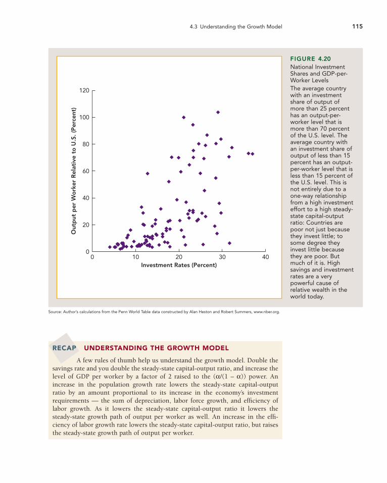
models but in reality? It turns out that it is important indeed, as Figure 4.20 shows.Of the 22 countries in the world with GDP-per-worker levels at least half of the U.S. level, 19 have investment shares of more than 20 percent of output. The highcapital-output ratios generated by high investment efforts are a very powerful sourceof relative prosperity in the world today.


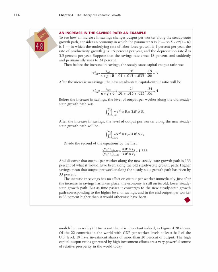
AN INCREASE IN THE SAVINGS RATE: AN EXAMPLETo see how an increase in savings changes output per worker along the steady-stategrowth path, consider an economy in which the parameter α is 1⁄2 — so λ = α/(1 – α)is 1 — in which the underlying rate of labor-force growth is 1 percent per year, therate of productivity growth g is 1.5 percent per year, and the depreciation rate δ is3.5 percent per year. Suppose that the savings rate s was 18 percent, and suddenlyand permanently rises to 24 percent.

Then before the increase in savings, the steady-state capital-output ratio was

After the increase in savings, the new steady-state capital-output ratio will be

Before the increase in savings, the level of output per worker along the old steady-state growth path was

After the increase in savings, the level of output per worker along the new steady-state growth path will be

Divide the second of the equations by the first:

And discover that output per worker along the new steady-state growth path is 133percent of what it would have been along the old steady-state growth path: Highersavings mean that output per worker along the steady-state growth path has risen by33 percent.

The increase in savings has no effect on output per worker immediately. Just afterthe increase in savings has taken place, the economy is still on its old, lower steady-state growth path. But as time passes it converges to the new steady-state growthpath corresponding to the higher level of savings, and in the end output per workeris 33 percent higher than it would otherwise have been.

(Yt / Lt)(Yt / Lt)

= 4.01 × Et

ss,old

ss,new

3.01 × Et = 1.333

Yt

Lt

=( Et = 4.01 × Et) ×ss,new

κ*λ

Yt

Lt

=( Et = 3.01 × Et) ×ss,old

κ*λ

newκ* = sn + g + δ

.24.01 + .015 + .035

= .24.06

= = 4new

oldκ* = sn + g + δ

.18.01 + .015 + .035

= .18.06

= = 3old

4.8BOX


Out

put

per

Wo

rker

Rel

ativ

e to

U.S

. (P

erce

nt)

120

100

80

60

40

20

0

Investment Rates (Percent)0 10 20 30 40

FIGURE 4.20National InvestmentShares and GDP-per-Worker Levels The average countrywith an investmentshare of output ofmore than 25 percenthas an output-per-worker level that ismore than 70 percentof the U.S. level. Theaverage country withan investment share ofoutput of less than 15percent has an output-per-worker level that isless than 15 percent ofthe U.S. level. This isnot entirely due to aone-way relationshipfrom a high investmenteffort to a high steady-state capital-outputratio: Countries arepoor not just becausethey invest little; tosome degree theyinvest little becausethey are poor. Butmuch of it is. Highsavings and investmentrates are a verypowerful cause ofrelative wealth in theworld today.

Source: Author’s calculations from the Penn World Table data constructed by Alan Heston and Robert Summers, www.nber.org.

RECAP UNDERSTANDING THE GROWTH MODEL

A few rules of thumb help us understand the growth model. Double thesavings rate and you double the steady-state capital-output ratio, and increase thelevel of GDP per worker by a factor of 2 raised to the (α/(1 – α)) power. An increase in the population growth rate lowers the steady-state capital-output ratio by an amount proportional to its increase in the economy’s investment requirements — the sum of depreciation, labor force growth, and efficiency oflabor growth. As it lowers the steady-state capital-output ratio it lowers thesteady-state growth path of output per worker as well. An increase in the effi-ciency of labor growth rate lowers the steady-state capital-output ratio, but raisesthe steady-state growth path of output per worker.

1. One principal force driving long-run growth in outputper worker is the set of improvements in the efficiencyof labor springing from technological progress.

2. A second principal force driving long-run growth inoutput per worker is the increases in the capital stockwhich the average worker has at his or her disposal andwhich further multiplies productivity.

3. An economy undergoing long-run growth converges toward and settles onto an equilibrium steady-state

growth path, in which the economy’s capital-outputratio is constant.

4. The steady-state level of the capital-output ratio is equalto the economy’s savings rate divided by the sum of itslabor-force growth rate, labor efficiency growth rate,and depreciation rate.


Chapter Summary

Key Termscapital intensity (p. 88)

efficiency of labor (p. 88)

production function (p. 90)

labor force (p. 90, 94)

capital (p. 90)

output per worker (p. 90)

savings rate (p. 96)

depreciation (p. 96)

capital-output ratio (p. 98)

convergence (p. 103)

steady-state growth path (p. 105)

Analytical Exercises1. Consider an economy in which the depreciation rate is

3 percent per year, the rate of population increase is 1percent per year, the rate of technological progress is 1percent per year, and the private savings rate is 16 per-cent of GDP. Suppose that the government increases itsbudget deficit — which had been at 1 percent of GDPfor a long time — to 3.5 percent of GDP and keeps itthere indefinitely.a. What will be the effect of this shift in policy on the

economy’s steady-state capital-output ratio?b. What will be the effect of this shift in policy on the

economy’s steady-state growth path for output perworker? How does your answer depend on the valueof the diminishing-returns-to-capital parameter α?

c. Suppose that your forecast of output per worker 20years in the future was $100,000. What is your newforecast of output per worker 20 years hence?

2. Suppose that a country has the production function

Yt = Kt0.5 × (Et × Lt)0.5

a. What is output Y considered as a function of the levelof the efficiency of labor E, the size of the labor forceL, and the capital-output ratio K/Y?

b. What is output per worker Y/L?

3. Suppose that with the production function

Yt = Kt0.5 × (Et × Lt)0.5

the depreciation rate on capital is 3 percent per year, therate of population growth is 1 percent per year, and therate of growth of the efficiency of labor is 1 percent peryear. a. Suppose that the savings rate is 10 percent of GDP.

What is the steady-state capital-output ratio? What isthe value of output per worker on the steady-stategrowth path written as a function of the level of theefficiency of labor?

b. Suppose that the savings rate is 15 percent of GDP.What is the steady-state capital-output ratio? What isthe value of output per worker on the steady-stategrowth path?

c. Suppose that the savings rate is 20 percent of GDP.What is the steady-state capital-output ratio? What isthe value of output per worker on the steady-stategrowth path?

4. What happens to the steady-state capital-output ratio ifthe rate of technological progress increases? Would the steady-state growth path of output per worker forthe economy shift upward, downward, or remain in thesame position?

5. Discuss the following proposition: “An increase in thesavings rate will increase the steady-state capital-outputratio and so increase both output per worker and therate of economic growth in both the short run and thelong run.”

6. Would the steady-state growth path of output perworker for the economy shift upward, downward, or re-main the same if capital were to become more durable— if the rate of depreciation on capital were to fall?

7. Suppose that a sudden disaster — an epidemic, say —reduces a country’s population and labor force but doesnot affect its capital stock. Suppose further that theeconomy was on its steady-state growth path before theepidemic.a. What is the immediate effect of the epidemic on out-

put per worker? On the total economywide level ofoutput?

b. What happens subsequently?

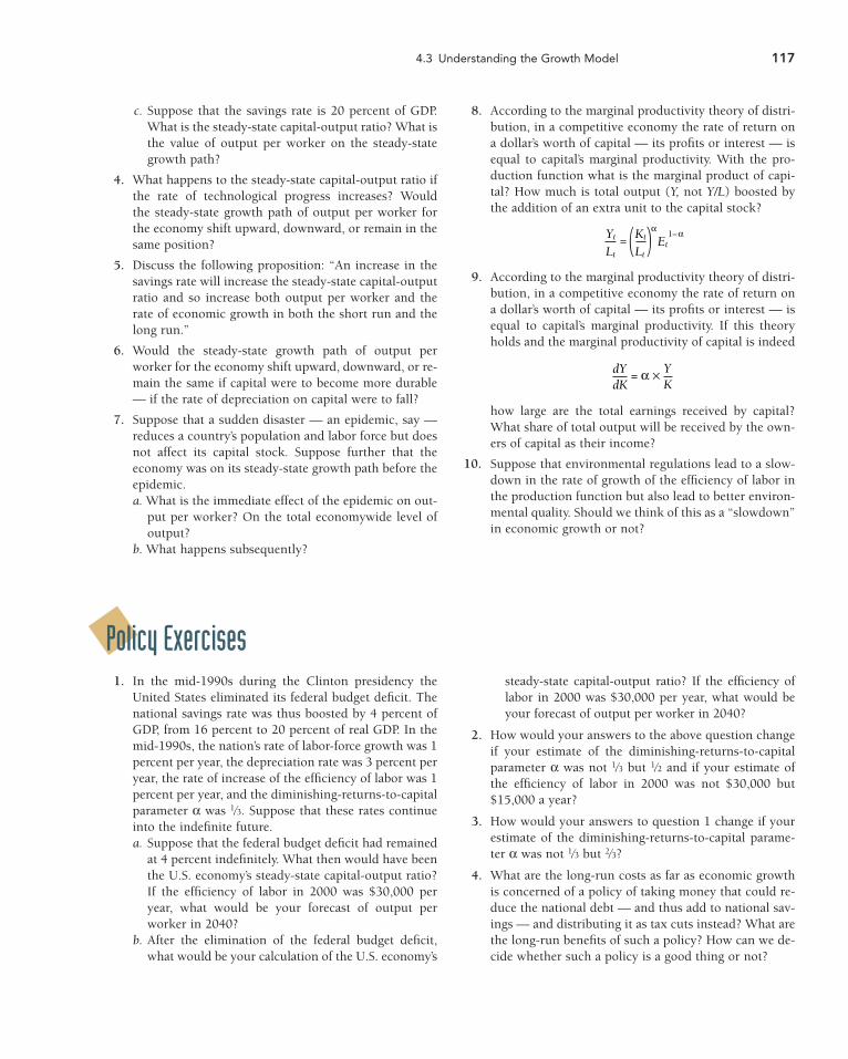
8. According to the marginal productivity theory of distri-bution, in a competitive economy the rate of return ona dollar’s worth of capital — its profits or interest — isequal to capital’s marginal productivity. With the pro-duction function what is the marginal product of capi-tal? How much is total output (Y, not Y/L) boosted bythe addition of an extra unit to the capital stock?

9. According to the marginal productivity theory of distri-bution, in a competitive economy the rate of return ona dollar’s worth of capital — its profits or interest — isequal to capital’s marginal productivity. If this theoryholds and the marginal productivity of capital is indeed

how large are the total earnings received by capital?What share of total output will be received by the own-ers of capital as their income?

10. Suppose that environmental regulations lead to a slow-down in the rate of growth of the efficiency of labor inthe production function but also lead to better environ-mental quality. Should we think of this as a “slowdown”in economic growth or not?

dYdK

YK

= α ×

Yt

Lt

Kt

Lt

= Et

α1–α( )


Policy Exercises1. In the mid-1990s during the Clinton presidency the

United States eliminated its federal budget deficit. Thenational savings rate was thus boosted by 4 percent ofGDP, from 16 percent to 20 percent of real GDP. In themid-1990s, the nation’s rate of labor-force growth was 1percent per year, the depreciation rate was 3 percent peryear, the rate of increase of the efficiency of labor was 1percent per year, and the diminishing-returns-to-capitalparameter α was 1⁄3. Suppose that these rates continueinto the indefinite future.a. Suppose that the federal budget deficit had remained

at 4 percent indefinitely. What then would have beenthe U.S. economy’s steady-state capital-output ratio?If the efficiency of labor in 2000 was $30,000 peryear, what would be your forecast of output perworker in 2040?

b. After the elimination of the federal budget deficit,what would be your calculation of the U.S. economy’s

steady-state capital-output ratio? If the efficiency oflabor in 2000 was $30,000 per year, what would beyour forecast of output per worker in 2040?

2. How would your answers to the above question changeif your estimate of the diminishing-returns-to-capitalparameter α was not 1⁄3 but 1⁄2 and if your estimate ofthe efficiency of labor in 2000 was not $30,000 but$15,000 a year?

3. How would your answers to question 1 change if yourestimate of the diminishing-returns-to-capital parame-ter α was not 1⁄3 but 2⁄3?

4. What are the long-run costs as far as economic growthis concerned of a policy of taking money that could re-duce the national debt — and thus add to national sav-ings — and distributing it as tax cuts instead? What arethe long-run benefits of such a policy? How can we de-cide whether such a policy is a good thing or not?

year, the rate of growth of the efficiency of labor was 2.5percent per year, and the savings rate was 16 percent ofGDP. The diminishing-returns-to-capital parameter α is0.5.a. What is Mexico’s steady-state capital-output ratio?b. Suppose that Mexico today is on its steady-state

growth path. What is the current level of the effi-ciency of labor E?

c. What is your forecast of output per worker in Mex-ico in 2040?

9. In the framework of the question above, how muchdoes your forecast of output per worker in Mexico in2040 increase if: a. Mexico’s domestic savings rate remains unchanged

but the nation is able to finance extra investmentequal to 4 percent of GDP every year by borrowingfrom abroad?

b. The labor-force growth rate immediately falls to 1percent per year?

c. Both a and b happen?

10. Consider an economy with a labor-force growth rate of2 percent per year, a depreciation rate of 4 percent peryear, a rate of growth of the efficiency of labor of 2 per-cent per year, and a savings rate of 16 percent of GDP. Ifthe savings rate increases from 16 to 17 percent, what isthe proportional increase in the steady-state level ofoutput per worker if the diminishing-returns-to-capitalparameter α is 1⁄3? 1⁄2? 2⁄3? 3⁄4?

5. At the end of the 1990s it appeared that because of thecomputer revolution the rate of growth of the efficiencyof labor in the United States had doubled, from 1 per-cent per year to 2 percent per year. Suppose this in-crease is permanent. And suppose the rate of labor-forcegrowth remains constant at 1 percent per year, the de-preciation rate remains constant at 3 percent per year,and the American savings rate (plus foreign capital in-vested in America) remains constant at 20 percent peryear. Assume that the efficiency of labor in the UnitedStates in 2000 was $15,000 per year and that the diminishing-returns-to-capital parameter α was 1⁄3.a. What is the change in the steady-state capital-output

ratio? What is the new capital-output ratio?b. Would such a permanent acceleration in the rate of

growth of the efficiency of labor change your forecastof the level of output per worker in 2040?

6. How would your answers to the above question changeif your estimate of the diminishing-returns-to-capitalparameter α was not 1⁄3 but 1⁄2 and if your estimate ofthe efficiency of labor in 2000 was not $30,000 but$15,000 a year?

7. How would your answers to question 5 change if yourestimate of the diminishing-returns-to-capital parame-ter α was not 1⁄3 but 2⁄3?

8. Output per worker in Mexico in the year 2000 wasabout $10,000 per year. Labor-force growth was 2.5 per-cent per year. The depreciation rate was 3 percent per


long-run economic growth - brad delong

Documents