Long-run relationships between international stock

prices: further evidence from fractional cointegration

tests

Marcel Aloy, Mohamed Boutahar, Karine Gente, Anne Peguin-Feissolle

To cite this version:

Marcel Aloy, Mohamed Boutahar, Karine Gente, Anne Peguin-Feissolle. Long-run relationshipsbetween international stock prices: further evidence from fractional cointegration tests. 2011.<halshs-00567472>

HAL Id: halshs-00567472

https://halshs.archives-ouvertes.fr/halshs-00567472

Submitted on 21 Feb 2011

HAL is a multi-disciplinary open accessarchive for the deposit and dissemination of sci-entific research documents, whether they are pub-lished or not. The documents may come fromteaching and research institutions in France orabroad, or from public or private research centers.

L’archive ouverte pluridisciplinaire HAL, estdestinee au depot et a la diffusion de documentsscientifiques de niveau recherche, publies ou non,emanant des etablissements d’enseignement et derecherche francais ou etrangers, des laboratoirespublics ou prives.

1

GREQAM Groupement de Recherche en Economie

Quantitative d'Aix-Marseille - UMR-CNRS 6579 Ecole des Hautes études en Sciences Sociales

Universités d'Aix-Marseille II et III

Document de Travail n°2011-07

Long-run relationships between international stock prices:

further evidence from fractional cointegration tests

Marcel Aloy Mohamed Boutahar

Karine Gente Anne Péguin-Feissolle

February 2011

Long-run relationships betweeninternational stock prices: further

evidence from fractional cointegrationtests

Marcel Aloy∗ Mohamed Boutahar† Karine Gente‡

Anne Péguin-Feissolle§

February 21, 2011

Abstract

The recent empirical literature supports the view that most ofthe international stock prices are not pairwise cointegrated. How-ever, by using fractional cointegration techniques, this paper showsthat France, Germany, Hong Kong, and Japan stock prices indices arepairwise fractionally cointegrated with US stock prices. Equilibriumerrors are mean reverting with half-life lying between 2 and 12 days. Itis worthwhile noting that emerging markets like Brazil and Argentinaare not pairwise cointegrated with the US stock market. These newresults have important implications for asset pricing and internationalportfolio strategy.

Keywords: equity markets, fractional cointegration, long memory

JEL classification: C12, C22, F31, F37, G15.

∗DEFI, Université de la Méditerranée, Faculté des Sciences Economiques et de Gestion,14 Avenue J. Ferry, 13621 Aix-en-Provence, FRANCE, Email: marcel.aloy@univmed.fr

†Corresponding author: Mohamed Boutahar, GREQAM, Université de la Méditerranée,Centre de la Charité, 2 rue de la Charite, 13236 Marseille cedex 02, FRANCE, Email:mohammed.boutahar@univmed.fr

‡DEFI, Université de la Méditerranée, Faculté des Sciences Economiques et de Gestion,14 Avenue J. Ferry, 13621 Aix-en-Provence, FRANCE, Email: karine.gente@univmed.fr

§GREQAM, CNRS, Centre de la Charité, 2 rue de la Charite, 13236 Marseille cedex02, FRANCE, Email: Anne.Peguin@univmed.fr

1

1 Introduction

A great number of papers have used cointegration techniques to examinethe long-run relationships between international stock prices, motivated bythe fact that cointegration between stock prices has several important im-plications for asset pricing. Firstly, cointegration between prices of somenational stock markets implies that these markets share a common stochas-tic trend. As a consequence, potential benefits from long run diversificationwill be reduced since deviations of one market away from the equilibriumrelationship can be expected to reverse geometrically over the long run. Sec-ondly, as stated by Granger (1986), evidence of cointegration among worldcapital markets may lead to the rejection of the efficient markets hypothe-sis since cointegration induces short run predictability of prices via the er-ror correction mechanism; however, Richards (1995), among others, arguesthat cointegration among stock prices may not necessarily imply violation ofmarket efficiency. Thirdly, some researchers have documented the long-runpredictability of prices through the Winner—Loser reversal effect (Richards,1995) which states that markets that have experienced superior performancecan be expected to underperform over the longer term, and vice versa.On the empirical side, the literature analyzing the long-run relationships

between international stock markets has produced mixed results. Some pa-pers (Kasa, 1992, Corhay et al., 1993, Dunis and Shannon, 2005; Fraser andOyefeso, 2005; Diamandis, 2009) found at least one common stochastic trendbetween international stock indices using Johansen’s (1988) multivariate lin-ear cointegration tests. However, the recent literature generally supports theview that most of the international stocks are not linearly pairwise cointe-grated (Chan et al., 1997; Kanas, 1998; Pynnönen and Knif, 1998; Huangand Fok, 2001; Davies, 2006; Li, 2006; Olusi and Abdul-Majid, 2008) or thatthe evidence for multivariate cointegration is weak1 (Ahlgren and Antell,2002). Focusing on UK (Taylor and Tonks, 1989), European stock markets(Rangvid, 2001; Garcia Pascual, 2003; Bley, 2009) or Pacific-Basin countries(Phylaktis and Ravazzolo, 2005), some papers suggest moreover that the inte-gration process of financial markets may be time and/or country dependent.An important reason for these mixed results is that usual linear testing

techniques may be inadequate in presence of non-standard dynamics, such asnonlinearity or structural change. Therefore, Li (2006) applies rank test fornon linear cointegration while Davies (2006) uses regime switching cointe-

1Ahlgren and Antell (2002) and Richards (1995) point out that some of the previousempirical results can be explained by the small-sample bias and size distortion of Jo-hansen’s LR tests for cointegration. Moreover, they underline the fact that Johansen’stests appear to be sensitive to the lag length specification in the VAR model.

2

gration techniques and Huang and Fok (2001) suggest that markets may betemporally cointegrated by using tests related to the stochastic permanentbreaks model.The aim of this paper is to provide further evidence on the pairwise

linkages between the US and some of the major foreign equity markets bytaking into account the fractional cointegration hypothesis2. According tothis hypothesis, the cointegration errors tend to revert back hyperbolically(and not geometrically) to some mean (or deterministic trend): as in thestandard cointegration framework, fractional cointegration introduces arbi-trage opportunities, since there is some predictability of prices in the long-run (Winner-Loser effect) as well as in the short-run (through the fraction-ally error-correction mechanism suggested by Granger, 1986). However, in astrategic (or static in the sense of Lucas) asset allocation perspective, frac-tional cointegration reduces the gain of portfolio diversification.In this paper we consider France, Germany, UK and Japan equity mar-

kets and some emerging countries’ equity markets like Argentina, Brazil andHong Kong. We will proceed in three steps. The first step consists in investi-gating the order of integration of each national stock index. In a second step,we use the strategy of Gil-Alana (2003) and Caporale and Gil-Alana (2004a,2004b) to consider the possibility of the series being pairwise fractionallycointegrated. The third step consists in measuring the persistence of shocksfor countries whose stock markets are related to the US one in the long-run.We confirm that all stock index series we consider are non-stationary I(1).Except for Germany, we find no standard cointegration between US stockmarket and the foreign stock markets into consideration, as already statedby Kanas (1998) for the case of France and UK. However, we conclude thatthe US stock market is fractionally cointegrated with the French, German,Japanese, UK and Hong Kong stock market indices. Conversely, the rela-tionship is neither significant for the US stock market and the Argentinianindex, nor for the US stock market and the Brazilian index. The persistenceis measured by the half-lives which lie between 1.88 and 11.88 days, depend-ing on the country considered. The highest half-life is the Japanese one, thelowest being the French one.The rest of the paper is organized as follows. The next section presents the

econometric method for detecting fractional integration and cointegration.The empirical application is carried out in Section 3 while Section 4 containssome concluding comments.

2The paper of Pynnönen and Knif (1998) constitutes a first attempt to apply thefractional cointegration hypothesis in the case of stock markets. Using the Cheung andLai’s (1993) fractional cointegration test in the case of two scandinavian stock markets,the authors found no evidence of fractional cointegration.

3

2 The econometric approach

2.1 Fractional integration and cointegration

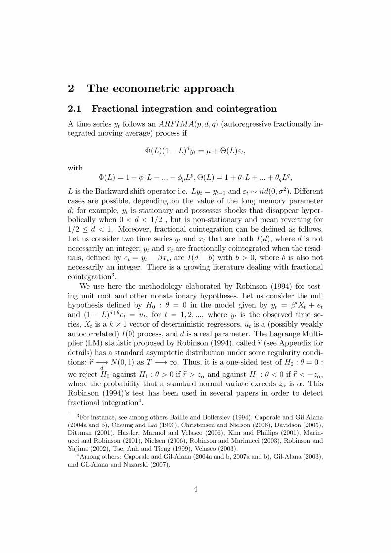
A time series yt follows an ARFIMA(p, d, q) (autoregressive fractionally in-tegrated moving average) process if

Φ(L)(1− L)dyt = μ+Θ(L)εt,

withΦ(L) = 1− φ1L− ...− φpL

p,Θ(L) = 1 + θ1L+ ...+ θqLq,

L is the Backward shift operator i.e. Lyt = yt−1 and εt ∼ iid(0, σ2). Differentcases are possible, depending on the value of the long memory parameterd; for example, yt is stationary and possesses shocks that disappear hyper-bolically when 0 < d < 1/2 , but is non-stationary and mean reverting for1/2 ≤ d < 1. Moreover, fractional cointegration can be defined as follows.Let us consider two time series yt and xt that are both I(d), where d is notnecessarily an integer; yt and xt are fractionally cointegrated when the resid-uals, defined by et = yt − βxt, are I(d − b) with b > 0, where b is also notnecessarily an integer. There is a growing literature dealing with fractionalcointegration3.We use here the methodology elaborated by Robinson (1994) for test-

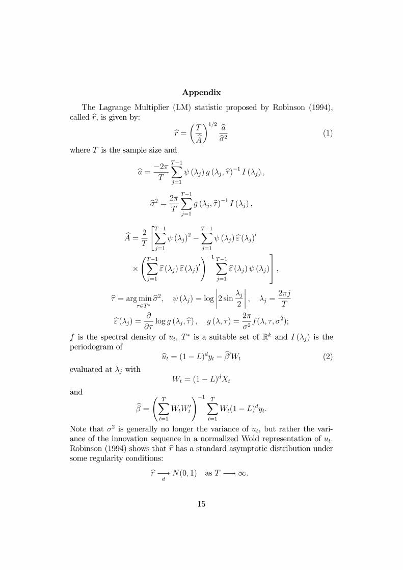
ing unit root and other nonstationary hypotheses. Let us consider the nullhypothesis defined by H0 : θ = 0 in the model given by yt = β0Xt + etand (1 − L)d+θet = ut, for t = 1, 2, ..., where yt is the observed time se-ries, Xt is a k × 1 vector of deterministic regressors, ut is a (possibly weaklyautocorrelated) I(0) process, and d is a real parameter. The Lagrange Multi-plier (LM) statistic proposed by Robinson (1994), called br (see Appendix fordetails) has a standard asymptotic distribution under some regularity condi-tions: br −→

dN(0, 1) as T −→∞. Thus, it is a one-sided test of H0 : θ = 0 :

we reject H0 against H1 : θ > 0 if br > zα and against H1 : θ < 0 if br < −zα,where the probability that a standard normal variate exceeds zα is α. ThisRobinson (1994)’s test has been used in several papers in order to detectfractional integration4.

3For instance, see among others Baillie and Bollerslev (1994), Caporale and Gil-Alana(2004a and b), Cheung and Lai (1993), Christensen and Nielson (2006), Davidson (2005),Dittman (2001), Hassler, Marmol and Velasco (2006), Kim and Phillips (2001), Marin-ucci and Robinson (2001), Nielsen (2006), Robinson and Marinucci (2003), Robinson andYajima (2002), Tse, Anh and Tieng (1999), Velasco (2003).

4Among others: Caporale and Gil-Alana (2004a and b, 2007a and b), Gil-Alana (2003),and Gil-Alana and Nazarski (2007).

4

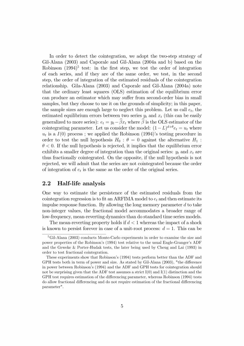
In order to detect the cointegration, we adopt the two-step strategy ofGil-Alana (2003) and Caporale and Gil-Alana (2004a and b) based on theRobinson (1994)5 test: in the first step, we test the order of integrationof each series, and if they are of the same order, we test, in the secondstep, the order of integration of the estimated residuals of the cointegrationrelationship. Gila-Alana (2003) and Caporale and Gil-Alana (2004a) notethat the ordinary least squares (OLS) estimation of the equilibrium errorcan produce an estimator which may suffer from second-order bias in smallsamples, but they choose to use it on the grounds of simplicity; in this paper,the sample sizes are enough large to neglect this problem. Let us call et, theestimated equilibrium errors between two series yt and xt (this can be easilygeneralized to more series): et = yt− bβxt where bβ is the OLS estimator of thecointegrating parameter. Let us consider the model: (1−L)d+θet = ut whereut is a I(0) process ; we applied the Robinson (1994)’s testing procedure inorder to test the null hypothesis H0 : θ = 0 against the alternative H1 :θ < 0. If the null hypothesis is rejected, it implies that the equilibrium errorexhibits a smaller degree of integration than the original series: yt and xt arethus fractionally cointegrated. On the opposite, if the null hypothesis is notrejected, we will admit that the series are not cointegrated because the orderof integration of et is the same as the order of the original series.

2.2 Half-life analysis

One way to estimate the persistence of the estimated residuals from thecointegration regression is to fit an ARFIMAmodel to et and then estimate itsimpulse response function. By allowing the long memory parameter d to takenon-integer values, the fractional model accommodates a broader range oflow-frequency, mean-reverting dynamics than do standard time series models.The mean-reverting property holds if d < 1 whereas the impact of a shock

is known to persist forever in case of a unit-root process: d = 1. This can be

5Gil-Alana (2003) conducts Monte-Carlo experiments in order to examine the size andpower properties of the Robinson’s (1994) test relative to the usual Engle-Granger’s ADFand the Geweke & Porter-Hudak tests, the later being used by Cheug and Lai (1993) inorder to test fractional cointegration.These experiments show that Robinson’s (1994) tests perform better than the ADF and

GPH tests both in term of power and size. As stated by Gil-Alana (2003), "the differencein power between Robinson’s (1994) and the ADF and GPH tests for cointegration shouldnot be surprising given that the ADF test assumes a strict I(0) and I(1) distinction and theGPH test requires estimation of the differencing parameter, whereas Robinson (1994) testsdo allow fractional differencing and do not require estimation of the fractional differencingparameter".

5

seen from the moving average representation for (1− L)et = A(L)εt where

A(L) = (1− L)1−dΨ(L) = 1 + a1L+ a2L2 + ....

Ψ(L) = 1 + ψ1L+ ψ2L2 + ....

The moving average coefficients aj, j = 1, ..., are referred to as the impulseresponses and can be computed as follows:

aj =

jXk=0

Γ(k + d− 1)Γ(d− 1)Γ(k + 1)ψj−k,

where the (ψj) can be computed recursively:

ψ0 = 1, ψj = θj +

min(j,p)Xi=1

φiψj−i if 1 ≤ j ≤ q

and

ψj =

min(j,p)Xi=1

φiψj−i if j ≥ q + 1.

The cumulative impulse response function over j periods of time is given byCj = 1+ a1 + ...+ aj and it tracks the impact of a unit innovation at time ton the long run equilibrium relationship at time t+j. As j →∞ C∞ = A(1),measuring the long-run impact of the innovation (Campbell and Mankiw,1987). Cheung and Lai (1993) show that for d < 1, C∞ = 0, implying shock-dissipating behavior. Conversely for d ≥ 1, C∞ 6= 0, the effect of a shockwill not die out. Mean reversion (i.e. C∞ = 0) occurs as long as d < 1.A measure of persistence usually considered in the literature is the half-life,which indicates how long it takes after a unit shock to dissipate by half onthe long-run equilibrium. The half-life can be computed from the Cj functionas t = h at where Ch = 0.5. For ARMA models, an analytical expressionfor the half-life can be derived; for example, it is well known that the half-life of the AR(1) model et = φet−1 + εt is given by h = − log(2)/ log(φ).However, for the ARFIMA model, the half-life remains difficult to compute.This problem can be solved plotting the impulse response function and usinglinear interpolation.

3 Empirical analysis

3.1 The data

The different series are the daily closing values for the following stock indices:BOV (Bovespa, Brazil), CAC (CAC 40, France), DAX (Dax, Germany),

6

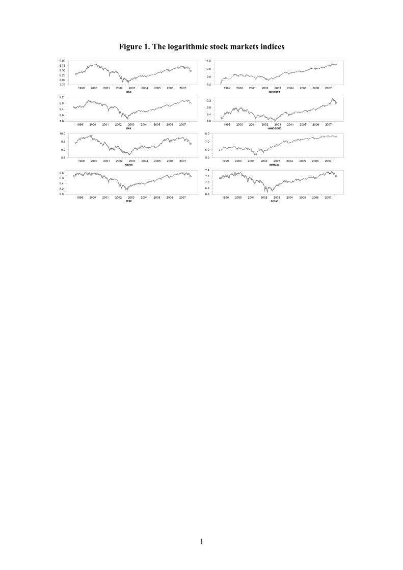
FTSE (FTSE 100, UK), HS (Hang Seng, Hong Kong), NK (Nikkei 225,Japan), MERV (Merval, Argentina) and SP (Standard and Poor’s 500,USA). We consider the log-transformed daily data over the period January4, 1999 - March 6, 2008 (T = 2389 where T is the sample size). The log-transformed daily series over the whole period are plotted in Figure 1 (thedescriptive statistics of the returns are given in Table 1).

[Insert Table 1 here][Insert Figure 1 here]

3.2 Empirical results

3.2.1 Integration analysis of individual series

The first step in the empirical analysis is to investigate the order of inte-gration of the individual series. We first perform the Kwiatowski, Phillips,Schmidt and Shin (1992) (KPSS) test for unit root, where the null hypoth-esis is the stationarity, on the raw series and on the first differenced series.The results are reported in Table 2 and clearly show the rejection of thenull hypothesis by the KPSS test on the raw series and the non-rejectionof the null hypothesis on the differenced series, which means that all thelog-transformed daily series contain a unit root.

[Insert Table 2 here]

Table 3 summarizes the results of the FELW estimation procedure (Shi-motsu (2006)) of the long memory parameter d, for the different series; bd arethe estimators of d and bσ are the estimated standard-errors; dl and du are thelower and upper bounds of the confidence intervals, respectively bd − 1.96bσand bd+1.96bσ. The orders of integration lies between 0.964 and 1.080, and theunit value lies always in the 95% confidence intervals, whatever the series; itconfirms again that the series contain a unit root, i.e., the null d = 1 cannotbe rejected.

[Insert Table 3 here]

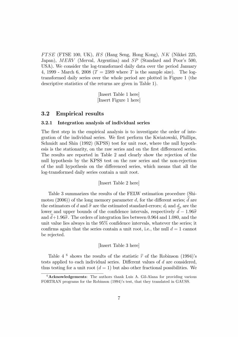
Table 4 6 shows the results of the statistic br of the Robinson (1994)’stests applied to each individual series. Different values of d are considered,thus testing for a unit root (d = 1) but also other fractional possibilities. We

6Acknowledgements: The authors thank Luis A. Gil-Alana for providing variousFORTRAN programs for the Robinson (1994)’s test, that they translated in GAUSS.

7

can observe that the minimum of the absolute values of the Robinson (1994)test statistic occurs always when d = 0.95 or 1 (and 1.05 for MERV ). Thispermits to conclude that all the series may contain a unit root or are closeto the unit root case.

[Insert Table 4 here]

3.2.2 Cointegration analysis

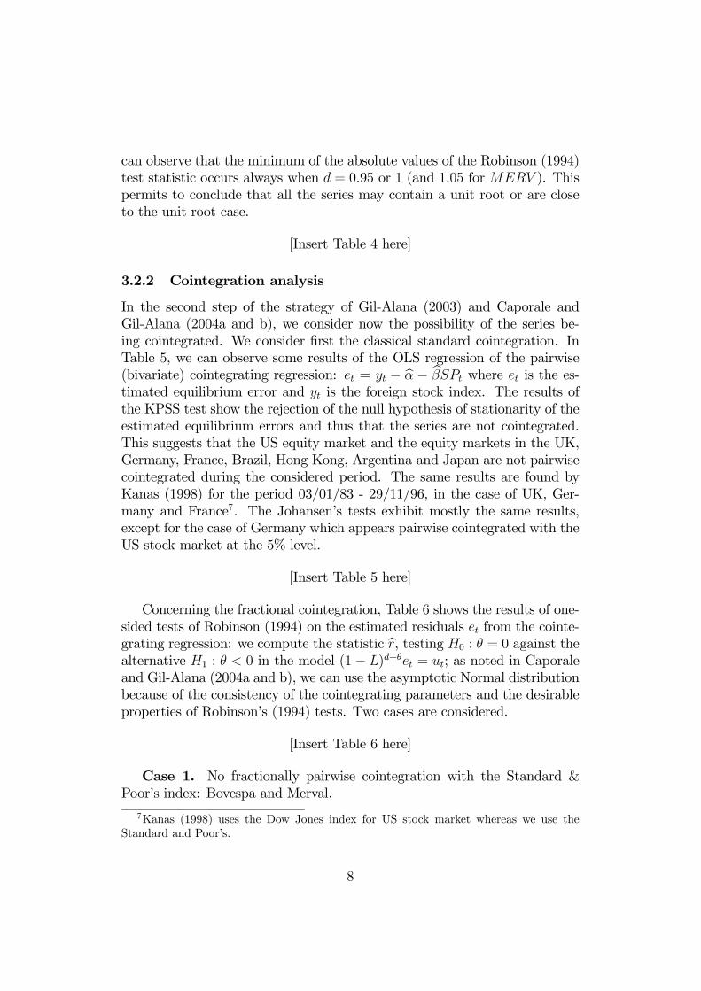
In the second step of the strategy of Gil-Alana (2003) and Caporale andGil-Alana (2004a and b), we consider now the possibility of the series be-ing cointegrated. We consider first the classical standard cointegration. InTable 5, we can observe some results of the OLS regression of the pairwise(bivariate) cointegrating regression: et = yt − bα − bβSPt where et is the es-timated equilibrium error and yt is the foreign stock index. The results ofthe KPSS test show the rejection of the null hypothesis of stationarity of theestimated equilibrium errors and thus that the series are not cointegrated.This suggests that the US equity market and the equity markets in the UK,Germany, France, Brazil, Hong Kong, Argentina and Japan are not pairwisecointegrated during the considered period. The same results are found byKanas (1998) for the period 03/01/83 - 29/11/96, in the case of UK, Ger-many and France7. The Johansen’s tests exhibit mostly the same results,except for the case of Germany which appears pairwise cointegrated with theUS stock market at the 5% level.

[Insert Table 5 here]

Concerning the fractional cointegration, Table 6 shows the results of one-sided tests of Robinson (1994) on the estimated residuals et from the cointe-grating regression: we compute the statistic br, testing H0 : θ = 0 against thealternative H1 : θ < 0 in the model (1− L)d+θet = ut; as noted in Caporaleand Gil-Alana (2004a and b), we can use the asymptotic Normal distributionbecause of the consistency of the cointegrating parameters and the desirableproperties of Robinson’s (1994) tests. Two cases are considered.

[Insert Table 6 here]

Case 1. No fractionally pairwise cointegration with the Standard &Poor’s index: Bovespa and Merval.

7Kanas (1998) uses the Dow Jones index for US stock market whereas we use theStandard and Poor’s.

8

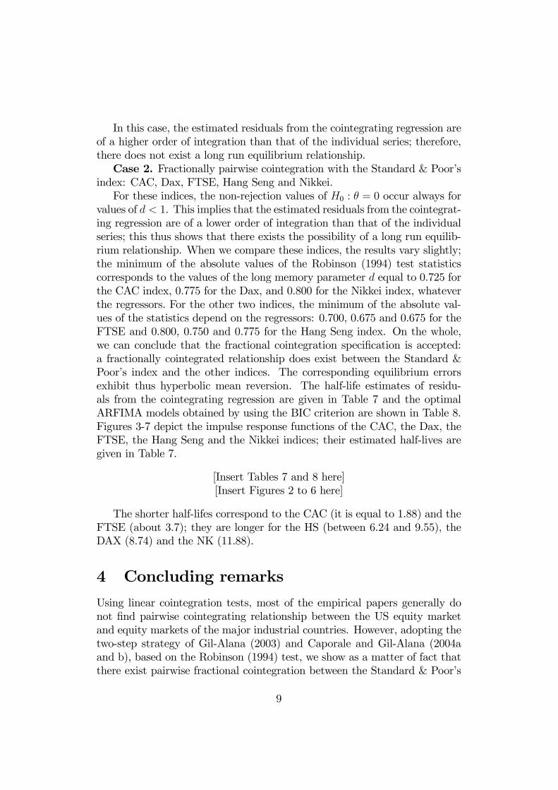
In this case, the estimated residuals from the cointegrating regression areof a higher order of integration than that of the individual series; therefore,there does not exist a long run equilibrium relationship.Case 2. Fractionally pairwise cointegration with the Standard & Poor’s

index: CAC, Dax, FTSE, Hang Seng and Nikkei.For these indices, the non-rejection values of H0 : θ = 0 occur always for

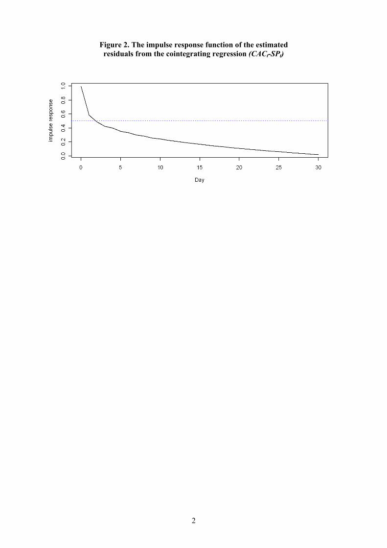
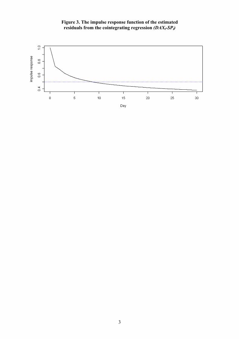
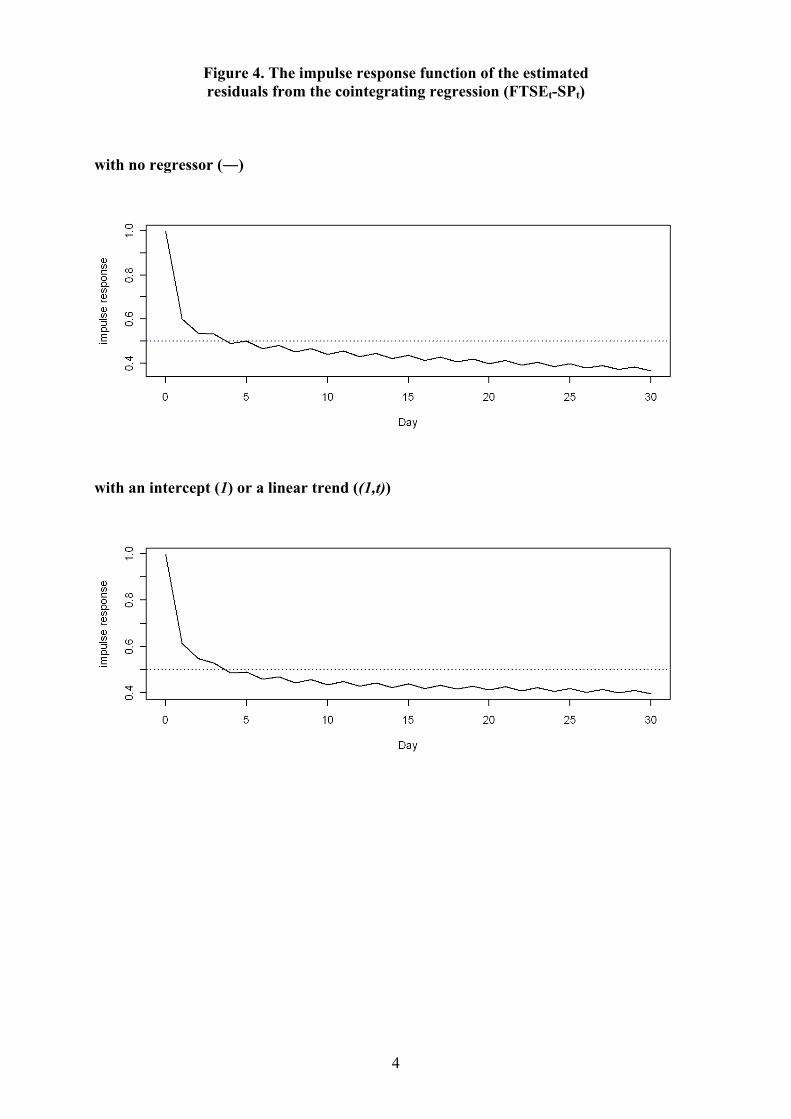
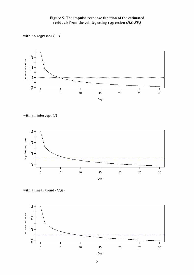
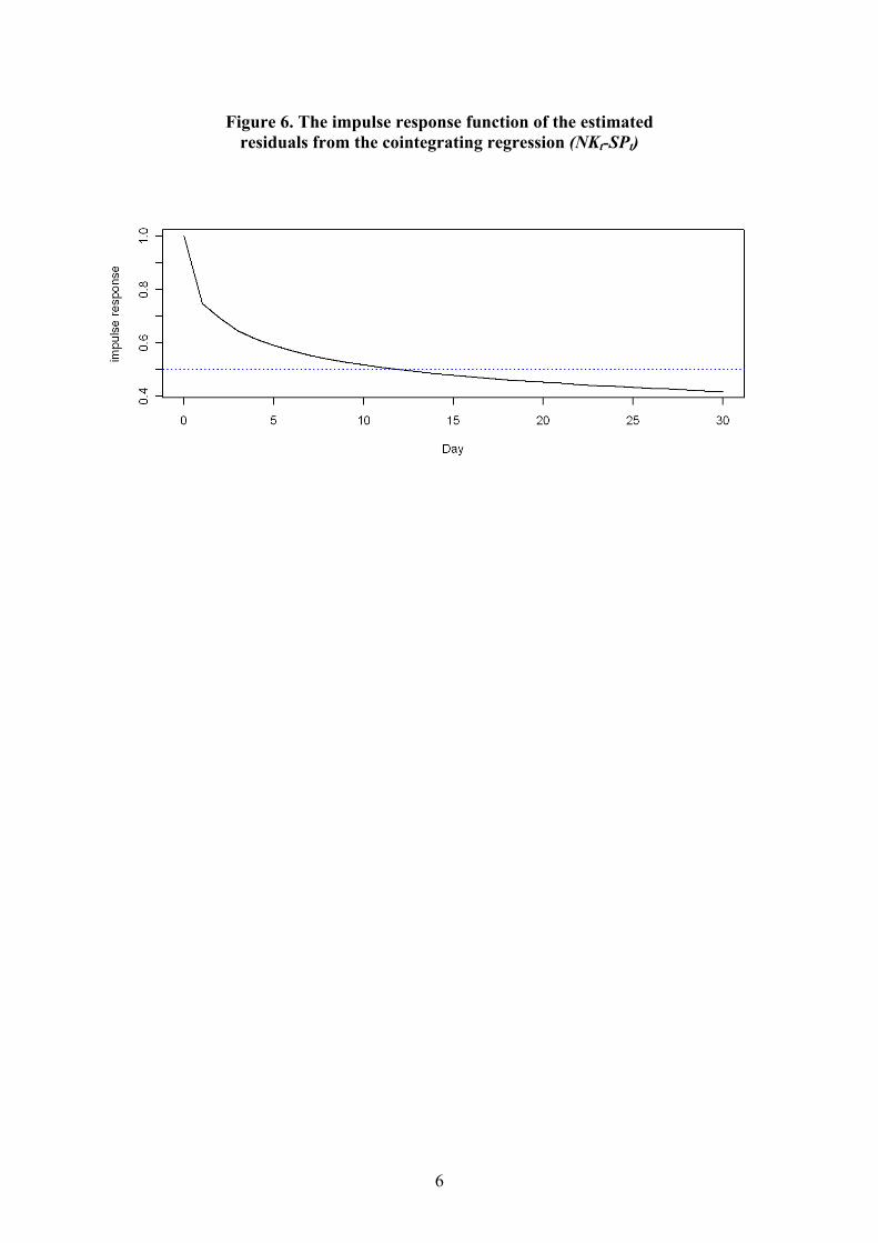
values of d < 1. This implies that the estimated residuals from the cointegrat-ing regression are of a lower order of integration than that of the individualseries; this thus shows that there exists the possibility of a long run equilib-rium relationship. When we compare these indices, the results vary slightly;the minimum of the absolute values of the Robinson (1994) test statisticscorresponds to the values of the long memory parameter d equal to 0.725 forthe CAC index, 0.775 for the Dax, and 0.800 for the Nikkei index, whateverthe regressors. For the other two indices, the minimum of the absolute val-ues of the statistics depend on the regressors: 0.700, 0.675 and 0.675 for theFTSE and 0.800, 0.750 and 0.775 for the Hang Seng index. On the whole,we can conclude that the fractional cointegration specification is accepted:a fractionally cointegrated relationship does exist between the Standard &Poor’s index and the other indices. The corresponding equilibrium errorsexhibit thus hyperbolic mean reversion. The half-life estimates of residu-als from the cointegrating regression are given in Table 7 and the optimalARFIMA models obtained by using the BIC criterion are shown in Table 8.Figures 3-7 depict the impulse response functions of the CAC, the Dax, theFTSE, the Hang Seng and the Nikkei indices; their estimated half-lives aregiven in Table 7.

[Insert Tables 7 and 8 here][Insert Figures 2 to 6 here]

The shorter half-lifes correspond to the CAC (it is equal to 1.88) and theFTSE (about 3.7); they are longer for the HS (between 6.24 and 9.55), theDAX (8.74) and the NK (11.88).

4 Concluding remarks

Using linear cointegration tests, most of the empirical papers generally donot find pairwise cointegrating relationship between the US equity marketand equity markets of the major industrial countries. However, adopting thetwo-step strategy of Gil-Alana (2003) and Caporale and Gil-Alana (2004aand b), based on the Robinson (1994) test, we show as a matter of fact thatthere exist pairwise fractional cointegration between the Standard & Poor’s

9

index and the CAC, the Dax, the FTSE, the Hang Seng and the Nikkeiindices; the corresponding equilibrium errors exhibit mean reversion, withhalf-life deviations lying between 2 and 12 days. It is worthwhile noting thatemerging markets like Brazil and Argentina are not fractionally cointegratedwith US stock market. These results suggest that there is some predictabilityof prices in the long-run (Winner-Loser effect) as well as in the short-runfor the stock markets of industrialized countries, but also this evidence offractional cointegration reduces, in the long-run, the potential benefits ofinternational portfolio diversification. However, another important result isthat these conclusions do not hold for some emerging countries.

References

[1] Ahlgren, N., Antell, J., 2002. Testing for cointegration between interna-tional stock prices, Applied Financial Economics 12, 851-861.

[2] Baillie, R.T., Bollerslev, T., 1994. Cointegration, fractional cointegra-tion, and exchange rate dynamics. The Journal of Finance 49, 737—745.

[3] Bley, J., 2009. European stock market integration: Fact or fiction?, Int.Fin. Markets, Inst. and Money 19, 759-776.

[4] Campbell, J.Y., Mankiw, N.G., 1987. Are output fluctuations transi-tory?. Quarterly Journal of Economics 102, 857—880.

[5] Caporale, G.M., Gil-Alana, L.A., 2004a. Fractional cointegration andtests of present value models. Review of Financial Economics 13, 245—258.

[6] Caporale, G.M., Gil-Alana, L.A., 2004b. Fractional cointegration andreal exchange rates. Review of Financial Economics 13, 327—340.

[7] Caporale, G.M., Gil-Alana, L.A., 2007a. Mean reversion in the US trea-sury constant maturity rates. Centre for International Capital Markets,Discussion Paper No 2007-5.

[8] Caporale G.M., Gil-Alana L.A., 2007b. Mean reversion in the Nikkei,Standard & Poor and Dow Jones stock market indices. Brunel Univer-sity, Discussion Paper.

[9] Chan, K.C., Gup, B.E., Pan, M-S., 1997. International stock market effi-ciency and integration: a study of eighteen nations, Journal of BusinessFinance & Accounting, 24(6).

10

[10] Cheung, Y.W., Lai, K.S., 1993. A fractional cointegration analysis ofpurchasing power parity. Journal of Business and Economic Statistics11, 103—112.

[11] Christensen, B., Nielson, M., 2006. Asymptotic normality of narrow-band least squares in the stationary fractional cointegration model andvolatility forecasting. Journal of Econometrics 133, 343-371.

[12] Corhay, A., Rad, A. T., Urbain, J.-P., 1993. Common Stochastic Trendsin European Stock Markets, Economics Letters 42, 385-390.

[13] Davidson, J., 2005. Testing for fractional cointegration: The relationshipbetween government popularity and economic performance in the UK.In: Diebolt, C., and Kyrtsou, C. (Eds.), New Trends in Macroeconomics.Springer Verlag.

[14] Davies, A., 2006. Testing for international equity market integrationusing regime switching cointegration techniques, Review of FinancialEconomics 15, 305—321.

[15] Diamandis, P.F., 2009. International stock market linkages: Evidencefrom Latin America, Global Finance Journal 20, 13—30.

[16] Dittman, I., 2001. Fractional cointegration of voting and non-votingshares. Applied Financial Economics 11, 321-332.

[17] Dunis, C.L., Shannon, G., 2005. Emerging markets of South-East andCentral Asia: Do they still offer a diversification benefit? Journal ofAsset Management, 6(3), 168—190.

[18] Fraser P., Oyefeso, O., 2005. US, UK and European Stock Market Inte-gration, Journal of Business Finance & Accounting, 32(1) & (2).

[19] Garcia Pascual, A., 2003. Assessing European stock markets(co)integration, Economics Letters 78, 197—203

[20] Geweke, J., Porter-Hudak, S., 1983. The estimation and application oflong memory time series models. Journal of Time Series Analysis 4 ,221-238.

[21] Gil-Alana, L.A., 2003. Testing of Fractional Cointegration in Macroeco-nomic Time Series, Oxford Bulletin of Economic and Statistics, 65(4)

11

[22] Gil-Alana, L.A., Nazarski, M., 2007. Strong dependence in the nominalexchange rates of the Polish zloty. Applied Stochastic Models in Businessand Industry 23, 97-116.

[23] Granger, C.W.J., 1986. Developments in the study of cointegrated eco-nomic variables, Oxford Bulletin of Economics and Statistics 48, 213-228.

[24] Hassler, U., Marmol, F., Velasco, C., 2006. Residual log-periodograminference for long run relationships. Journal of Econometrics 130, 165-207.

[25] Huang, B-N., Fok, C.W., 2001. Stock market integration: an applicationof the stochastic permanent breaks model, Applied Economics Letters8, 725-729.

[26] Johansen, S., 1988 Statistical analysis of cointegration vectors, Journalof Economics Dynamics and Control, 12, 231-54.

[27] Kanas, A., 1998. Linkages between the US and European equity markets:further evidence from cointegration tests. Applied Financial Economics8, 607-614.

[28] Kasa, K., 1992. Common Stochastic Trends in International Stock Mar-kets. Journal of Monetary Economics 29, 95-124.

[29] Kim, C., Phillips, P.C.B., 2001. Fully modified estimation of fractionalcointegration models. Yale University.

[30] Kwiatowski, D., Phillips, P.C.B., Schmidt, P, Shin, Y., 1992. Testingthe Null Hypothesis of Stationarity Against the Alternative of a UnitRoot: How Sure Are We That Economic Time Series Have a Unit Root?.Journal of Econometrics 54, 159-178.

[31] Li, X-M., 2006. A revisit of international stock market linkages: newevidence from rank tests for nonlinear cointegration, Scottish Journal ofPolitical Economy, Vol. 53, No. 2.

[32] Marinucci, D., Robinson, P.M., 2001. Semiparametric fractional cointe-gration analysis. Journal of Econometrics 105, 225-247.

[33] Nielsen, M., 2006. Local whittle analysis of stationary fractional cointe-gration and the implied realized volatility relation. Journal of Businessand Economics Statistics, forthcoming.

12

[34] Olusi, O., Abdul-Majid, H., 2008. Diversification prospects in MiddleEast and North Africa (MENA) equity markets: a synthesis and anupdate, Applied Financial Economics 18, 1451—1463.

[35] Phylaktis, K., Ravazzolo, F., 2005. Stock market linkages in emergingmarkets:implications for international portfolio diversification, Int. Fin.Markets, Inst. and Money 15, 91—106.

[36] Pynnonen S., Knif, J., 1998. Common long-term and short-term pricememory in two Scandinavian stock markets, Applied Financial Eco-nomics 8, 257-265.

[37] Rangvid, J., 2001. Increasing convergence among European stock mar-kets? A recursive common stochastic trends analysis, Economics Letters71, 383—389.

[38] Richards A.J., 1995. Comovements in national stock market returns:Evidence of predictability, but not cointegration, Journal of MonetaryEconomics 36, 631-654

[39] Robinson, P.M., 1994. Efficient tests of nonstationary hypotheses. Jour-nal of the American Statistical Association 89, 1420-1437.,

[40] Robinson, P.M., Marinucci, D., 2003. Semiparametric frequency domainanalysis of fractional cointegration. In: Robinson, P.M., (Ed.). TimeSeries with Long Memory. Oxford University Press, Oxford, 334—373.

[41] Robinson, P.M., Yajima, Y., 2002. Determination of cointegration rankin fractional systems. Journal of Econometrics 106, 217—241.

[42] Shimotsu, K., 2006. Exact local Whittle estimation of fractional inte-gration with unknown mean and time trend. Working Paper N. 1061,Queen’s University, Canada.

[43] Shin, Y., 1994. A residual based-test of the null of cointegration againstthe alternative of no cointegration. Econometric Theory 10, 91-115.

[44] Taylor, M. P., Tonks, I., 1989. The Internationalisation of Stock Marketsand the Abolition of U.K. Exchange Control. Review of Economics andStatistics 71, 332-336.

[45] Tse, Y., Anh, V., Tieng, A., 1999. No-cointegration test based on frac-tional differencing: Some Monte Carlo results. Journal of StatisticalPlanning and Inference 80, 257-267.

13

[46] Velasco, C., 2003. Gaussian semiparametric estimation of fractional coin-tegration. Journal of Time Series Analysis 24, 345-378.

14

Appendix

The Lagrange Multiplier (LM) statistic proposed by Robinson (1994),called br, is given by:

br = µTbA¶1/2 babσ2 (1)

where T is the sample size and

ba = −2πT

T−1Xj=1

ψ (λj) g (λj, bτ)−1 I (λj) ,bσ2 = 2π

T

T−1Xj=1

g (λj, bτ)−1 I (λj) ,bA = 2

T

"T−1Xj=1

ψ (λj)2 −

T−1Xj=1

ψ (λj) bε (λj)0×Ã

T−1Xj=1

bε (λj) bε (λj)0!−1 T−1Xj=1

bε (λj)ψ (λj)⎤⎦ ,

bτ = argmin bσ2τ∈T∗

, ψ (λj) = log

¯2 sin

λj2

¯, λj =

2πj

T

bε (λj) = ∂

∂τlog g (λj, bτ) , g (λ, τ) =

2π

σ2f(λ, τ, σ2);

f is the spectral density of ut, T ∗ is a suitable set of Rk and I (λj) is theperiodogram of but = (1− L)dyt − bβ0Wt (2)

evaluated at λj withWt = (1− L)dXt

and bβ = Ã TXt=1

WtW0t

!−1 TXt=1

Wt(1− L)dyt.

Note that σ2 is generally no longer the variance of ut, but rather the vari-ance of the innovation sequence in a normalized Wold representation of ut.Robinson (1994) shows that br has a standard asymptotic distribution undersome regularity conditions:br −→

dN(0, 1) as T −→∞.

15

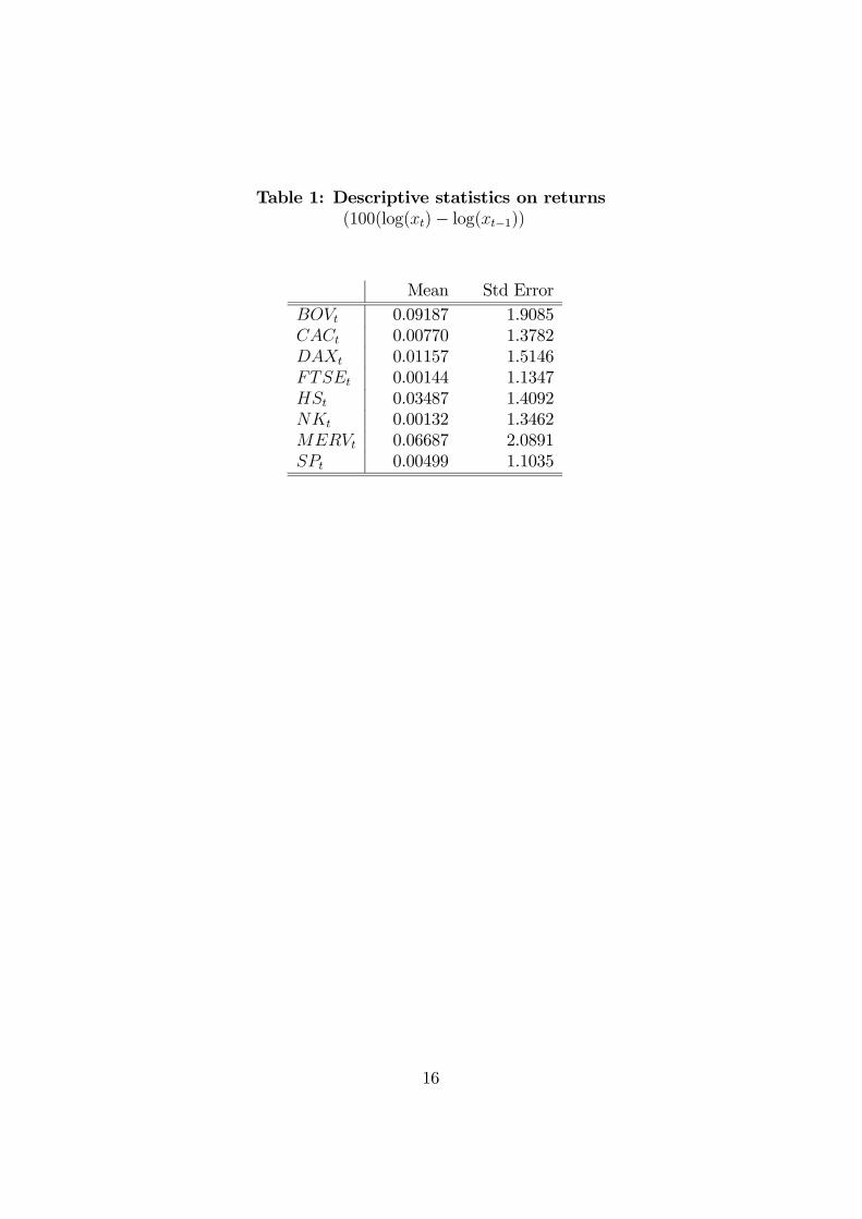
Table 1: Descriptive statistics on returns(100(log(xt)− log(xt−1))

Mean Std ErrorBOVt 0.09187 1.9085CACt 0.00770 1.3782DAXt 0.01157 1.5146FTSEt 0.00144 1.1347HSt 0.03487 1.4092NKt 0.00132 1.3462MERVt 0.06687 2.0891SPt 0.00499 1.1035

16

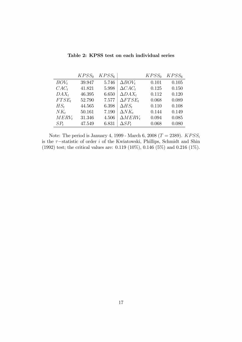
Table 2: KPSS test on each individual series

KPSS0 KPSS6 KPSS0 KPSS6BOVt 39.947 5.746 ∆BOVt 0.101 0.105CACt 41.821 5.998 ∆CACt 0.125 0.150DAXt 46.395 6.650 ∆DAXt 0.112 0.120FTSEt 52.790 7.577 ∆FTSEt 0.068 0.089HSt 44.565 6.398 ∆HSt 0.110 0.108NKt 50.161 7.190 ∆NKt 0.144 0.149MERVt 31.346 4.506 ∆MERVt 0.094 0.085SPt 47.549 6.831 ∆SPt 0.068 0.080

Note: The period is January 4, 1999 - March 6, 2008 (T = 2389). KPSSiis the τ−statistic of order i of the Kwiatowski, Phillips, Schmidt and Shin(1992) test; the critical values are: 0.119 (10%), 0.146 (5%) and 0.216 (1%).

17

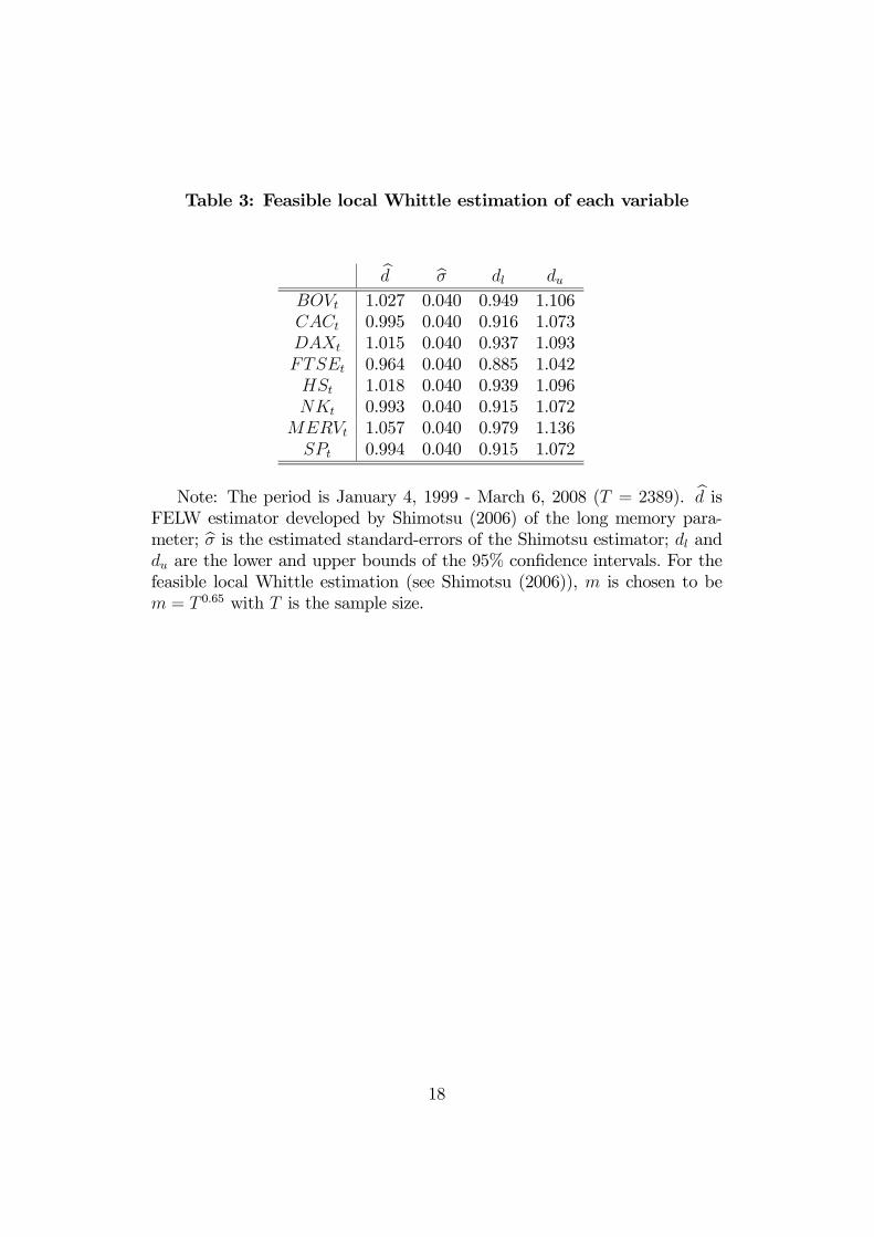
Table 3: Feasible local Whittle estimation of each variable

bd bσ dl duBOVt 1.027 0.040 0.949 1.106CACt 0.995 0.040 0.916 1.073DAXt 1.015 0.040 0.937 1.093FTSEt 0.964 0.040 0.885 1.042HSt 1.018 0.040 0.939 1.096NKt 0.993 0.040 0.915 1.072

MERVt 1.057 0.040 0.979 1.136SPt 0.994 0.040 0.915 1.072

Note: The period is January 4, 1999 - March 6, 2008 (T = 2389). bd isFELW estimator developed by Shimotsu (2006) of the long memory para-meter; bσ is the estimated standard-errors of the Shimotsu estimator; dl anddu are the lower and upper bounds of the 95% confidence intervals. For thefeasible local Whittle estimation (see Shimotsu (2006)), m is chosen to bem = T 0.65 with T is the sample size.

18

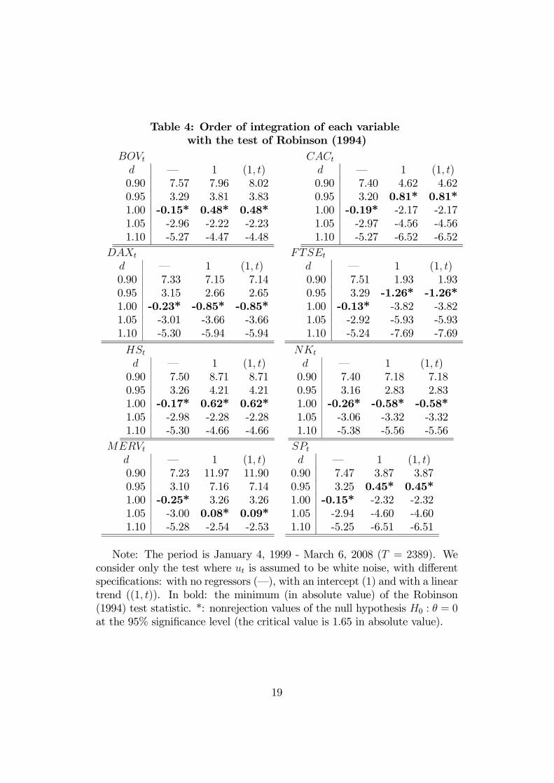
Table 4: Order of integration of each variablewith the test of Robinson (1994)

BOVtd – 1 (1, t)0.90 7.57 7.96 8.020.95 3.29 3.81 3.831.00 -0.15* 0.48* 0.48*1.05 -2.96 -2.22 -2.231.10 -5.27 -4.47 -4.48

CACt

d – 1 (1, t)0.90 7.40 4.62 4.620.95 3.20 0.81* 0.81*1.00 -0.19* -2.17 -2.171.05 -2.97 -4.56 -4.561.10 -5.27 -6.52 -6.52

DAXt

d – 1 (1, t)0.90 7.33 7.15 7.140.95 3.15 2.66 2.651.00 -0.23* -0.85* -0.85*1.05 -3.01 -3.66 -3.661.10 -5.30 -5.94 -5.94

FTSEt

d – 1 (1, t)0.90 7.51 1.93 1.930.95 3.29 -1.26* -1.26*1.00 -0.13* -3.82 -3.821.05 -2.92 -5.93 -5.931.10 -5.24 -7.69 -7.69

HStd – 1 (1, t)0.90 7.50 8.71 8.710.95 3.26 4.21 4.211.00 -0.17* 0.62* 0.62*1.05 -2.98 -2.28 -2.281.10 -5.30 -4.66 -4.66

NKt

d – 1 (1, t)0.90 7.40 7.18 7.180.95 3.16 2.83 2.831.00 -0.26* -0.58* -0.58*1.05 -3.06 -3.32 -3.321.10 -5.38 -5.56 -5.56

MERVtd – 1 (1, t)0.90 7.23 11.97 11.900.95 3.10 7.16 7.141.00 -0.25* 3.26 3.261.05 -3.00 0.08* 0.09*1.10 -5.28 -2.54 -2.53

SPt

d – 1 (1, t)0.90 7.47 3.87 3.870.95 3.25 0.45* 0.45*1.00 -0.15* -2.32 -2.321.05 -2.94 -4.60 -4.601.10 -5.25 -6.51 -6.51

Note: The period is January 4, 1999 - March 6, 2008 (T = 2389). Weconsider only the test where ut is assumed to be white noise, with differentspecifications: with no regressors (–), with an intercept (1) and with a lineartrend ((1, t)). In bold: the minimum (in absolute value) of the Robinson(1994) test statistic. *: nonrejection values of the null hypothesis H0 : θ = 0at the 95% significance level (the critical value is 1.65 in absolute value).

19

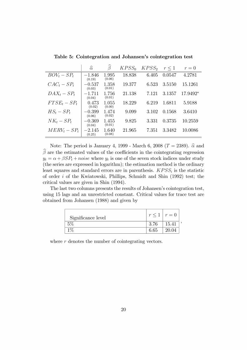
Table 5: Cointegration and Johansen’s cointegration test

bα bβ KPSS0 KPSS2 r ≤ 1 r = 0

BOVt − SPt −1.846(0.19)

1.995(0.06)

18.838 6.405 0.0547 4.2781

CACt − SPt −0.537(0.03)

1.358(0.01)

19.377 6.523 3.5150 15.1261

DAXt − SPt −1.711(0.04)

1.756(0.01)

21.138 7.121 3.1357 17.9492∗

FTSEt − SPt 0.473(0.02)

1.055(0.00)

18.229 6.219 1.6811 5.9188

HSt − SPt −0.399(0.06)

1.474(0.02)

9.099 3.102 0.1568 3.6410

NKt − SPt −0.369(0.04)

1.455(0.01)

9.825 3.331 0.3735 10.2559

MERVt − SPt −2.145(0.25)

1.640(0.08)

21.965 7.351 3.3482 10.0086

Note: The period is January 4, 1999 - March 6, 2008 (T = 2389). bα andbβ are the estimated values of the coefficients in the cointegrating regressionyt = α+βSPt+noise where yt is one of the seven stock indices under study(the series are expressed in logarithm); the estimation method is the ordinaryleast squares and standard errors are in parenthesis. KPSSi is the statisticof order i of the Kwiatowski, Phillips, Schmidt and Shin (1992) test; thecritical values are given in Shin (1994).The last two columns presents the results of Johansen’s cointegration test,

using 15 lags and an unrestricted constant. Critical values for trace test areobtained from Johansen (1988) and given by

Significance levelr ≤ 1 r = 0

5% 3.76 15.411% 6.65 20.04

,

where r denotes the number of cointegrating vectors.

20

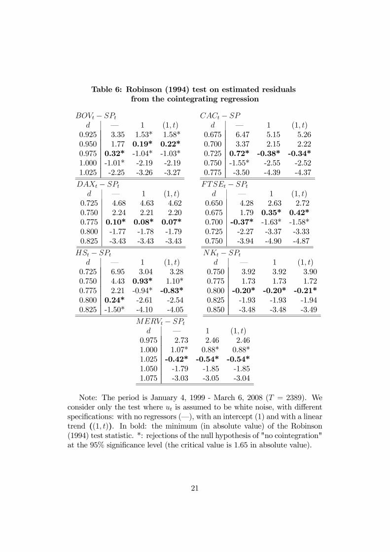
Table 6: Robinson (1994) test on estimated residualsfrom the cointegrating regression

BOVt − SPt

d – 1 (1, t)0.925 3.35 1.53* 1.58*0.950 1.77 0.19* 0.22*0.975 0.32* -1.04* -1.03*1.000 -1.01* -2.19 -2.191.025 -2.25 -3.26 -3.27

CACt − SPd – 1 (1, t)

0.675 6.47 5.15 5.260.700 3.37 2.15 2.220.725 0.72* -0.38* -0.34*0.750 -1.55* -2.55 -2.520.775 -3.50 -4.39 -4.37

DAXt − SPt

d – 1 (1, t)0.725 4.68 4.63 4.620.750 2.24 2.21 2.200.775 0.10* 0.08* 0.07*0.800 -1.77 -1.78 -1.790.825 -3.43 -3.43 -3.43

FTSEt − SPt

d – 1 (1, t)0.650 4.28 2.63 2.720.675 1.79 0.35* 0.42*0.700 -0.37* -1.63* -1.58*0.725 -2.27 -3.37 -3.330.750 -3.94 -4.90 -4.87

HSt − SPt

d – 1 (1, t)0.725 6.95 3.04 3.280.750 4.43 0.93* 1.10*0.775 2.21 -0.94* -0.83*0.800 0.24* -2.61 -2.540.825 -1.50* -4.10 -4.05

NKt − SPt

d – 1 (1, t)0.750 3.92 3.92 3.900.775 1.73 1.73 1.720.800 -0.20* -0.20* -0.21*0.825 -1.93 -1.93 -1.940.850 -3.48 -3.48 -3.49

MERVt − SPt

d – 1 (1, t)0.975 2.73 2.46 2.461.000 1.07* 0.88* 0.88*1.025 -0.42* -0.54* -0.54*1.050 -1.79 -1.85 -1.851.075 -3.03 -3.05 -3.04

Note: The period is January 4, 1999 - March 6, 2008 (T = 2389). Weconsider only the test where ut is assumed to be white noise, with differentspecifications: with no regressors (–), with an intercept (1) and with a lineartrend ((1, t)). In bold: the minimum (in absolute value) of the Robinson(1994) test statistic. *: rejections of the null hypothesis of "no cointegration"at the 95% significance level (the critical value is 1.65 in absolute value).

21

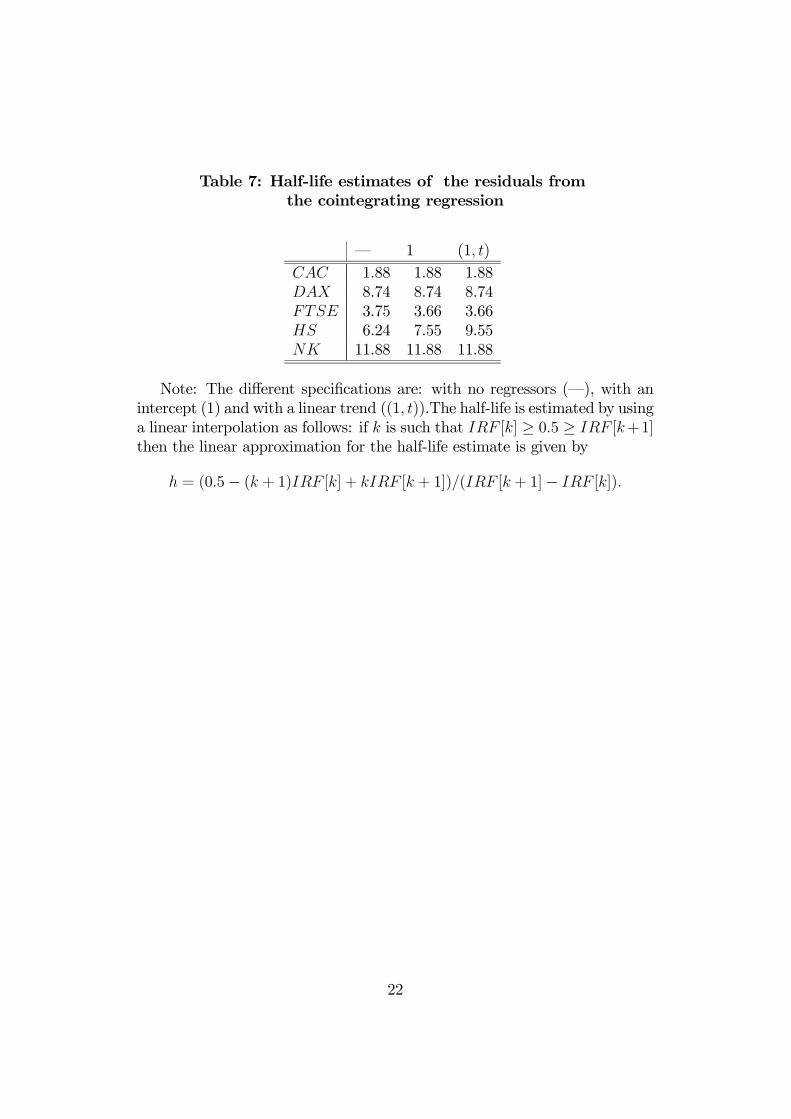
Table 7: Half-life estimates of the residuals fromthe cointegrating regression

– 1 (1, t)

CAC 1.88 1.88 1.88DAX 8.74 8.74 8.74FTSE 3.75 3.66 3.66HS 6.24 7.55 9.55NK 11.88 11.88 11.88

Note: The different specifications are: with no regressors (–), with anintercept (1) and with a linear trend ((1, t)).The half-life is estimated by usinga linear interpolation as follows: if k is such that IRF [k] ≥ 0.5 ≥ IRF [k+1]then the linear approximation for the half-life estimate is given by

h = (0.5− (k + 1)IRF [k] + kIRF [k + 1])/(IRF [k + 1]− IRF [k]).

22

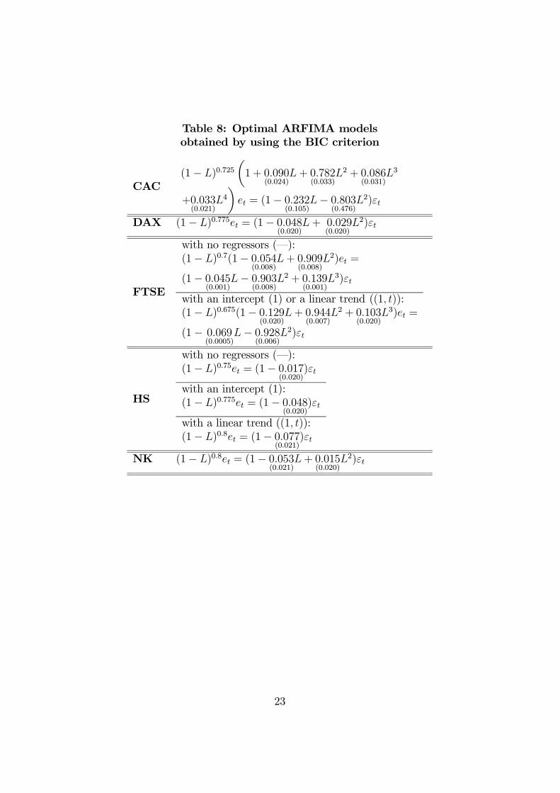
Table 8: Optimal ARFIMA modelsobtained by using the BIC criterion

CAC(1− L)0.725

µ1 + 0.090

(0.024)L+ 0.782

(0.033)L2 + 0.086

(0.031)L3

+0.033(0.021)

L4¶et = (1− 0.232

(0.105)L− 0.803

(0.476)L2)εt

DAX (1− L)0.775et = (1− 0.048(0.020)

L+ 0.029(0.020)

L2)εt

FTSE

with no regressors (–):(1− L)0.7(1− 0.054

(0.008)L+ 0.909

(0.008)L2)et =

(1− 0.045(0.001)

L− 0.903(0.008)

L2 + 0.139(0.001)

L3)εt

with an intercept (1) or a linear trend ((1, t)):(1− L)0.675(1− 0.129

(0.020)L+ 0.944

(0.007)L2 + 0.103

(0.020)L3)et =

(1− 0.069(0.0005)

L− 0.928(0.006)

L2)εt

HS

with no regressors (–):(1− L)0.75et = (1− 0.017

(0.020))εt

with an intercept (1):(1− L)0.775et = (1− 0.048

(0.020))εt

with a linear trend ((1, t)):(1− L)0.8et = (1− 0.077

(0.021))εt

NK (1− L)0.8et = (1− 0.053(0.021)

L+ 0.015(0.020)

L2)εt

23

1

Figure 1. The logarithmic stock markets indices

CAC1999 2000 2001 2002 2003 2004 2005 2006 2007

7.75

8.00

8.25

8.50

8.75

9.00

DAX1999 2000 2001 2002 2003 2004 2005 2006 2007

7.6

8.0

8.4

8.8

9.2

NIKKEI1999 2000 2001 2002 2003 2004 2005 2006 2007

8.8

9.2

9.6

10.0

FTSE1999 2000 2001 2002 2003 2004 2005 2006 2007

8.0

8.2

8.4

8.6

8.8

BOVESPA1999 2000 2001 2002 2003 2004 2005 2006 2007

8.5

9.5

10.5

11.5

HANG SENG1999 2000 2001 2002 2003 2004 2005 2006 2007

9.0

9.4

9.8

10.2

MERVAL1999 2000 2001 2002 2003 2004 2005 2006 2007

5.0

6.0

7.0

8.0

SP5001999 2000 2001 2002 2003 2004 2005 2006 2007

6.6

6.8

7.0

7.2

7.4

2

Figure 2. The impulse response function of the estimated

residuals from the cointegrating regression (CACt-SPt)

3

Figure 3. The impulse response function of the estimated residuals from the cointegrating regression (DAXt-SPt)

4

Figure 4. The impulse response function of the estimated residuals from the cointegrating regression (FTSEt-SPt)

with no regressor (―)

with an intercept (1) or a linear trend ((1,t))

5

Figure 5. The impulse response function of the estimated residuals from the cointegrating regression (HSt-SPt)

with no regressor (―)

with an intercept (1)

with a linear trend ((1,t))

6

Figure 6. The impulse response function of the estimated residuals from the cointegrating regression (NKt-SPt)