long-term contracts under the threat of supplier default
TRANSCRIPT
Long-Term Contracts under the Threat ofSupplier Default
Robert Swinney � Serguei Netessine
The Wharton School, University of Pennsylvania, Philadelphia, PA, 19104
[email protected] � [email protected]
August, 2007. Forthcoming in Manufacturing & Service Operations Management.
Contracting with suppliers prone to default is an increasingly common problem in someindustries, particularly automotive manufacturing. We model this phenomenon as a twoperiod contracting game with two identical suppliers, a single buyer, deterministic demand,and uncertain production costs. The suppliers are distressed at the start of the game anddo not have access to external sources of capital, hence revenues from the buyer are crucialin determining whether or not default occurs. The production cost of each supplier is thesum of two stochastic components: a common term that is identical for both suppliers(representing raw materials costs, design speci�cations, etc.), and an idiosyncratic term thatis unique to a given supplier (representing inherent �rm capability). The buyer chooses asupplier and then decides on a single or two period contract. Comparing models with andwithout the possibility of default, we �nd that without the possibility of supplier failure, thebuyer always prefers short-term contracts over long-term contracts, whereas this preference istypically reversed in the presence of failure. Neither of these contracts coordinates the supplychain. We also consider dynamic contracts, in which the contract price is partially tied tosome index representing the common component of production costs (e.g., commodity pricesof raw materials such as steel or oil), allowing the buyer to shoulder some of the risk fromcost uncertainty. We �nd that dynamic long-term contracts allow the buyer to coordinatethe supply chain in the presence of default risk. We also demonstrate that our resultscontinue to hold under a variety of alternative assumptions, including stochastic demand,allowing the buyer the option of subsidizing a bankrupt supplier via a contingent transferpayment or loan, and allowing the buyer to unilaterally renegotiate contracts. We concludethat the possibility of supplier default o¤ers a new reason to prefer long-term contracts overshort-term contracts.
1. Introduction
The relationship between manufacturers and suppliers in the American automotive industry
is not always a cooperative one. American carmakers are on a perpetual quest to match the
procurement costs of their competitors by increasing supply chain e¢ ciency. Throughout
1
the 1990�s, an increased awareness of the value of cooperative buyer-supplier relationships
sparked interest in fostering strategic partnerships between automotive manufacturers and
suppliers. Nevertheless, despite the perceived value of collaborative behavior with suppliers,
auto manufacturers often engage in adversarial and caustic supplier management tactics,
typically employing one tool more than any other: direct pressure to reduce procurement
prices.
In the 1990�s, for example, Ford famously dictated an across-the-board 5% price decrease
to all of its suppliers (Stallkamp 2005). In 2005, Lear, a key seat supplier to Chrysler,
attempted to negotiate higher prices to cover recent sharp cost increases that plagued the
automotive supplier base. When Lear threatened to cease shipping products to Chrysler,
the automaker promptly took the supplier to court to enforce the terms of their contract,
despite the fact that Lear posted a net loss of nearly $600 million in the fourth quarter of
2005 alone. This emphasis on low procurement prices has had a clear adverse e¤ect on the
suppliers, however: pro�t margins are low across the industry, and many suppliers routinely
lose money (Wernle 2006a, Wynn 2006). In 2005, Delphi, the largest supplier of automotive
parts in the country, was in bankruptcy, as were numerous smaller suppliers.
While the poor �nancial health of the suppliers is exacerbated by the low procurement
costs demanded by automakers in response to the competitive North American automotive
landscape, there are several additional factors that have played a key role in the current
perilous state of the automotive supplier base. Bo Andersson, General Motors Vice President
for Global Purchasing and Supply Chain, cites four critical issues: production cost increases,
unstable domestic volume, legacy pension plans (resulting in larger overhead expenses), and
di¢ cult access to capital (Andersson 2006). The analysis that we present will touch upon
each of these key factors.
From a buyer�s point of view, losing a supplier to bankruptcy can have varying conse-
quences: on one extreme, if the supplier ceases operations, the buyer may have to switch
to a new supplier (possibly at a higher cost), whereas at another extreme, if the supplier
continues normal operations without disruption, the buyer may have to help support the
supplier �nancially, as was the case in some of the most visible supplier bankruptcies of
2005 (e.g., Delphi, see Nussel and Barkholz 2006). When interior parts supplier Collins &
Aikman entered bankruptcy in 2005, automakers had little choice but to sustain the supplier�
roughly 90% of vehicles made in North America have at least one component produced by
the supplier�and the estimated total cost to the Big Three auto manufacturers was $532
2
million, resulting from the cancellation of loan repayments, parts price increases, operating
subsidies, and legal fees (Barkholz and Sherefkin 2007).
Thus, the possibility of losing a supplier to failure may a¤ect the decisions that a buyer
makes, including the price and the length of contracts. Should a buyer pay more to avoid
losing a supplier to bankruptcy, or should the buyer pay less because the supplier is risky?
Should the buyer make a long-term commitment to the supplier, or should the �rm minimize
the length of its exposure to a risky partner? Should buyers bear some of the risk of cost
uncertainty by compensating suppliers in a dynamic manner? These are the trade-o¤s we
seek to capture, via an operationalized model of buyer-supplier relations under the threat
of supplier failure. The motivation is the automotive industry, but the model is relevant to
many scenarios: supply chains with members in �nancial distress, supply chains with start-
ups prone to bankruptcy, etc. Based on the aforementioned examples from the automotive
industry, we believe these types of relationships have several key characteristics:
1. Uncertain Supplier Production Costs. Tooling and capacity installation lead-
times tend to be long and hence the buyer must commit to the supplier well in advance
of the �nalized design of the component. In addition, raw materials costs are uncertain
and often have a large impact on the supplier�s margins; Standard & Poor�s June 2006
industry survey of autos and auto parts cites high raw materials costs as a key factor
in the current distressed state of the supplier base (Levy and Ferazani 2006). Thus,
the actual per unit production cost to the supplier is unknown at the time of contract-
ing. We assume that this risk is not diversi�able because it derives from volatility
not captured in any current futures market (e.g., outputs from higher tier suppliers or
inherent uncertainty in design and production techniques). Even risk in raw materials
prices cannot always be hedged�Sherefkin (2006) describes how Ford has struggled to
create a futures market for automotive sheet steel.
2. Strong Bargaining Power of the Buyer. The buyer tends to be a large �rm
with most of the bargaining power while the supplier is the smaller �rm at risk of
default. For example, in the American auto industry, parts suppliers have few potential
buyers and face weak bargaining positions and low pro�t margins, while in Europe the
situation is far less bleak for the suppliers (Lewin 2006). Hence, the buyer has most of
the bargaining power and o¤ers the contract to the supplier, choosing both price and
the length of the contract.
3
3. Extended Sales Horizons. The product being supplied will be used over several
sales periods (e.g., a particular model of a car tends to be sold for 5-7 years before a
major redesign). Since the cost of switching suppliers is typically high (due to large
asset speci�c investments made by the manufacturers into a particular supplier), the
�nancial health of a dedicated supplier over the sales horizon is critical to the buyer.
Furthermore, the buyer has the option of contracting with a supplier for a single sale
period, or for multiple periods; both practices are observed in the auto industry (Dyer
1996).
These three points form the core of our model. In what follows, the goal is to analyze and
evaluate the performance of both long- and short-term contracts when suppliers face a risk
of failure, and to determine under what conditions a particular contract type is preferred.
We compare these results to a model with no supplier failure in which short-term contracts
are always preferred, and �nd that under the threat of supplier default this preference is
typically reversed. We further consider dynamic contracts, which partially compensate
the suppliers for the realized value of production costs, and �nd that long-term dynamic
contracts perform better than static contracts and are capable of achieving the centralized
system optimal pro�t.
Our results complement the existing literature on the value of long-term contracts in
supply chains by demonstrating their advantages despite controlling for many of the typical
reasons a buyer would have to prefer these contracts. For example, the management liter-
ature often discusses long-term relationships or contracts as a method of developing trust
between buyers and suppliers, but we do not consider any trust issues; indeed, the long-
term contracts are preferred even though the buyer is completely self-interested. Similarly,
long-term relationships are known to induce otherwise unsupportable actions in repeated
games, thus increasing their value relative to short-term relationships; in our model, the
value comes not from inducing actions but rather from reducing the expected cost of sup-
plier default to the buyer. Overall, we o¤er a new reason to employ long-term contracts: to
reduce the damage from supplier default. Our �nding is consistent with current practices
in the Japanese auto industry, in which long-term relationships are common and supplier
defaults are, relative to the U.S., uncommon.
The remainder of this paper is organized as follows: the next section provides a brief
literature review, and §3 describes the model. §4 analyzes a benchmark model with suppliers
4
that never enter bankruptcy, and §5 considers suppliers prone to bankruptcy. §6 explores a
class of contracts which partially compensate the suppliers for production costs in a dynamic
fashion. §7 discusses three interesting extensions (demand uncertainty, contingent transfer
payments, and normally distributed costs), and §8 concludes the paper.
2. Literature Review
There are three broad areas of research which are relevant to our paper. The �rst focuses
speci�cally on understanding the nature of buyer-supplier relationships in the auto industry,
while the second is primarily theoretical, concerning such issues as repeated contracting
between �rms, relational agreements, and contracting under cost uncertainty. The third
area of research focuses on the e¤ects of �nancial distress and supplier disruption risk.
There is a strong tradition, particularly in the management literature, of research into
the types of relationships that exist between buyers and suppliers in the automotive industry.
Tang (1999) provides an excellent discussion. Much of this work focuses on the historical
and current di¤erences between Japanese-style and American-style supply networks; see, for
example, McMillan (1990), Dyer et al. (1998), Dyer (1996), and references therein. The
traditional Japanese networks of suppliers, called keiretsu, are markedly di¤erent from their
American counterparts. The former are characterized by fewer suppliers, long-term relation-
ships, and heavy cooperation, while the latter traditionally utilized a large number of small
suppliers, short-term contracts, and non-cooperative or adversarial behavior. Japanese �rms
are often heavily invested in their suppliers, wholly or partly owning their closest partners
in many instances (Dyer et al. 1998), and even when buyers are not directly invested in
suppliers, there is indirect investment via the value of the ongoing relationship. Such close
networks of suppliers inextricably link the �nancial health of �rms in the supply chain.
Empirically, there is evidence both that the �nancial health of suppliers matters to buyers
and that collaborative relationships are bene�cial to suppliers. Choi and Hartley (1996), in a
survey of suppliers and automakers in the US industry, �nd that �nancial issues are a primary
factor in supplier selection, and furthermore that greater importance is placed on �nancial
health by downstream �rms (i.e., the auto assemblers) than by upstream �rms. Srinivasan
and Brush (2006) �nd empirical evidence (outside of the auto industry) that buyer-supplier
collaboration and target pricing bene�t the �nancial performance of suppliers.
5
Thus, in recent years, American companies have attempted to emulate some aspects of
the Japanese system, in particular the narrowing of supplier bases and longer term contracts;
see, for example, Dyer (1996), Tang (1999), and more recently Wernle (2006b). Neverthe-
less, as Sako and Helper (1998) demonstrate, trust between supply chain partners is still
higher among Japanese �rms than among American �rms. Furthermore, Rudambi and
Helper (1998) �nd empirical evidence for non-cooperative behavior in the U.S. auto indus-
try, suggesting that signi�cant di¤erences still persist between the American and Japanese
auto industries. Consequently, a buyer only has incentive to keep suppliers in good �nancial
standing if it bene�ts the buyer through lower costs. This is precisely the situation that we
model: a non-cooperative supplier-buyer relationship in which the buyer is concerned with
the failure of a supplier only to the extent that it might be costly for the buyer to switch
suppliers.
We will examine two scenarios: a long-term contract that covers the entire horizon, and
a series of repeated, short-term contracts. Li and Debo (2005) examine a similar model,
quantifying the value of commitment to a single �rm in a two period newsvendor context in
which suppliers have private information about their production costs. The buyer runs an
auction to pick a supplier, and may choose to run an auction in each period or to commit to a
supplier in the �rst period. They �nd that a long-term contract increases the aggressiveness
of supplier bidding, and thus helps to counteract the e¤ect of information asymmetry. While
the results of Li and Debo (2005) are driven by information asymmetries, our model is
driven by failure risk and cost uncertainty; ex ante, there is no information asymmetry in
our setting.
The short-term contracts in our model are essentially relational contracts, which consti-
tute an emerging topic in the operations literature. The term �relational contract�refers to
the fact that the enforcement of the contract comes from the value of the future relationship
rather than from direct legal enforcement. Examples of related papers include Taylor and
Plambeck (2003) and Atkins et al. (2005). These models contain single-buyer, single-supplier
relationships, in contrast to our own model with two suppliers. Tunca and Zenios (2006), on
the other hand, examine a model of repeated contracting with multiple suppliers and buyers.
The authors compare relational contracts for high quality components with and without a
secondary electronic market for low quality components. Their model, in contrast to ours,
has a powerful high-quality supplier who both o¤ers the contract to the buyer and does so
before a group of low-quality suppliers (i.e., the high-quality supplier is a Stackelberg leader).
6
None of these papers considers the endogenous e¤ect of one partner leaving the relationship
due to failure, high production costs, low capital, etc. (although discount factors in repeated
games can be thought of as an exogenous probability of relationship termination).
There is also a related literature comparing long- and short-term contracts under cost
uncertainty, surveyed by Kleindorfer and Wu (2003). In much of this literature, long-term
contracts refer to those signed prior to the realization of some random variable (e.g., cost
or demand) and short-term contracts are those signed after the realization of this stochastic
event, with demand usually occurring in a single period. One exception is the multiperiod
model of Cohen and Agrawal (1999); however, in contrast to our own model, contract price
is not a decision variable (although contract length is) and there is no chance of contract
termination due to supplier default. For a general reference on contracting in supply chains,
we refer to the survey by Cachon (2003).
Papers that have considered �rm bankruptcy or failure in an operational context are
Archibald et al. (2002) and Swinney et al. (2005). Both of these papers de�ne failure in
the same way as the present work: if capital falls below a prespeci�ed level, the �rm ceases
to exist. The �rst paper looks at a monopoly setting, while the latter considers duopolies.
Neither consider contracting e¤ects between �rms.
In a closely related paper, Babich et al. (2005) analyze a model with multiple suppliers
and a single buyer, wherein suppliers face an exogenous probability of default and act as
Stackelberg leaders in setting the wholesale price for a downstream newsvendor. Our model
di¤ers in that the default risk is endogenous (i.e., it is a function of the contract price between
buyer and supplier, implying the buyer�s business has a signi�cant e¤ect on the supplier�s
�nancial health) and the bargaining power lies with the buyer. Furthermore, Babich et al.
(2005) consider a single period model, whereas our model considers contracting e¤ects over
multiple periods. Related papers include Babich (2006).
Tomlin (2006) considers methods of mitigating disruption risk when the buyer may con-
tract with reliable and unreliable suppliers. The focus is on sourcing and contingency
strategies to help mitigate the e¤ects of disruption risk under uncertain demand, whereas
our focus is on contract parameters that directly minimize the buyer�s expenses from supplier
failure under uncertain costs. In much of the disruption risk literature, the risk of failure or
default is exogenous, whereas in our analysis, it is endogenously determined by the contract
price between the buyer and the supplier. To summarize, we are not aware of any work that,
like ours, uses contracting to mitigate the harmful e¤ects of endogenous supplier default.
7
3. The Model
There are two identical suppliers (subscript i = 1; 2) and a single buyer (subscript b). The
analysis is unchanged if we consider a pool of an arbitrary number of potential (ex-ante
identical) suppliers. The buyer requires some critical component in each of two periods,
and will contract with one supplier at a time in order to obtain the component. We
assume that dual sourcing is too costly to be considered (i.e., there is a large �xed cost
to doing business with any supplier); Tang (1999) describes how American companies have
recently reduced supplier bases and increased the frequency of sole-sourcing to control costs.
Demand is identical and known in each period and without loss of generality is normalized to
one, consistent with the automotive industry, in which short-term forecasts of sales (and, in
particular, of procurement quantities from suppliers) are fairly accurate for mature products.
(We will relax the assumption of deterministic demand in §7.1.) The buyer sells the �nished
product for price s.
Each supplier has a linear unit production cost that is the sum of two independent
stochastic components: common costs ct, t = 1; 2, which are identical for both suppliers
but may be time dependent, and idiosyncratic costs di, i = 1; 2 that are unique to a given
supplier but may be correlated with one another, and are constant across time. Thus,
the total production cost of supplier i at time t is ct + di. For generality, we allow both
random variables to have support in (�1;1), though they may be restricted to some smallerinterval. The uncertainty in common cost arises from stochastic elements that a¤ect both
�rms: for example, raw materials costs or product design speci�cations. The uncertainty in
a �rm�s idiosyncratic cost arises from factors unique to a given supplier, such as the e¢ ciency
of a supplier�s production facilities or its level of technical expertise, re�ecting an implicit
notion of cost discovery in the production process; suppliers may have some estimate about
their inherent e¢ ciency, but until they physically produce a large number of units, the precise
value of this cost is unknown.
All �rms have identical beliefs that c1 has distribution F (�), unimodal density f (�), and�nite mean �1 > 0. The second period common cost may depend on the realized value of
the �rst period cost. The conditional mean is de�ned as �2(x) = E (c2jc1 = x), and theunconditional mean is �2 > 0, and both are assumed to be �nite.
The idiosyncratic costs of the two suppliers may be correlated; however, since the sup-
pliers are assumed to be ex-ante identical, the marginal distributions are identical as well,
8
and all �rms thus have beliefs that the marginal cdf is G (x) and the marginal pdf is g (x).
The conditional mean is �d (x) = E (d2jd1 = x) and the unconditional mean is �d > 0, whereboth are assumed to be �nite. The correlation coe¢ cient between d1 and d2 is denoted
�d. For technical reasons, we assume that x � �d (x) is monotonically increasing. (The
complementary case of x��d (x) monotonically decreasing in x is impossible if the marginaldistributions of d1 and d2 are identical.) For example, this assumption holds if d1 and d2
are bivariate normal.
There is no private information in the model; all parties learn the values of all random
variables when they are realized. For example, if supplier 1 produces in the �rst period, then
by the start of the second period both suppliers and the buyer know the values of c1 and d1.
The second period common cost and d2 are still unknown at this point, though the realized
value of d1 may convey some information about d2 if the two have non-zero correlation.
Our assumption of no private information comes for a variety of reasons re�ective of the
automotive industry: for example, sources of common cost uncertainty are clearly known
well by the buyer (e.g., raw materials, design speci�cations), while the buyer is also likely
to have a good estimate of the idiosyncratic capabilities of each supplier from existing (or
previous) relationships (in the auto industry, given the limited number of suppliers, it is
unlikely that a buyer has never worked with a given supplier in the past). Finally, most
suppliers are public companies and much of the labor is unionized, meaning the general
�nancial state of each supplier and labor costs are public information.
We assume that both suppliers are distressed at the start of the game; that is, they are
already in danger of bankruptcy when the buyer o¤ers a contract at the start of period one.
Suppliers are already heavily leveraged at the time of contract signing, and hence cannot
borrow additional funds from external sources (though it may be desirable to borrow or
transfer funds from the buyer; this is discussed in §7.2). Payments on outstanding debt
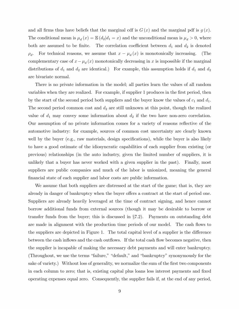
are made in alignment with the production time periods of our model. The cash �ows to
the suppliers are depicted in Figure 1. The total capital level of a supplier is the di¤erence
between the cash in�ows and the cash out�ows. If the total cash �ow becomes negative, then
the supplier is incapable of making the necessary debt payments and will enter bankruptcy.
(Throughout, we use the terms �failure,��default,�and �bankruptcy�synonymously for the
sake of variety.) Without loss of generality, we normalize the sum of the �rst two components
in each column to zero; that is, existing capital plus loans less interest payments and �xed
operating expenses equal zero. Consequently, the supplier fails if, at the end of any period,
9
In OutExisting Capital Interest Payment
Loans Fixed Operating ExpensesRevenue from Buyer Production Expenses
Figure 1. Cash �ows to the suppliers in each period.
the total pro�t from operations with the buyer falls below the bankruptcy threshold of zero.
If the supplier fails, then the relationship with the buyer is broken, and the buyer must
switch to a new supplier incurring a switching cost of k � 0. If the buyer chooses to switchsuppliers after one period of production, the same switching cost k is incurred. Alternatively,
k may be interpreted as a �xed setup cost incurred upon doing business with any supplier.
This value also includes any additional costs incurred by the buyer to expedite production
with the alternative supplier.
The expected pro�t to the buyer is �b, and the expected pro�t to supplier i is �i. We
assume that the buyer maximizes expected pro�t, and that supplier i agrees to any contract
with expected pro�t no less than the reservation level of zero. Non-zero reservation levels
and bankruptcy thresholds merely add constant terms to the contract parameters and do not
alter the qualitative nature of the results, and so for notational simplicity they are omitted.
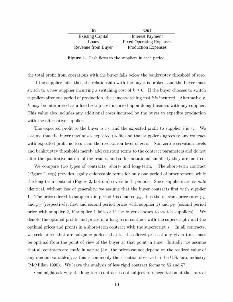
We compare two types of contracts: short- and long-term. The short-term contract
(Figure 2, top) provides legally enforceable terms for only one period of procurement, while
the long-term contract (Figure 2, bottom) covers both periods. Since suppliers are ex-ante
identical, without loss of generality, we assume that the buyer contracts �rst with supplier
1. The price o¤ered to supplier i in period t is denoted pit, thus the relevant prices are: p11
and p12 (respectively, �rst and second period prices with supplier 1) and p22 (second period
price with supplier 2, if supplier 1 fails or if the buyer chooses to switch suppliers). We
denote the optimal pro�ts and prices in a long-term contract with the superscript l and the
optimal prices and pro�ts in a short-term contract with the superscript s. In all contracts,
we seek prices that are subgame perfect�that is, the o¤ered price at any given time must
be optimal from the point of view of the buyer at that point in time. Initially, we assume
that all contracts are static in nature (i.e., the prices cannot depend on the realized value of
any random variables), as this is commonly the situation observed in the U.S. auto industry
(McMillan 1990). We leave the analysis of less rigid contract forms to §6 and §7.
One might ask why the long-term contract is not subject to renegotiation at the start of
10
Period 1 Period 2
Buyer offers aprice p11 tosupplier 1
Supplier 1 produces
Supplier 1 fails ifprofit is negative
Buyer chooses a supplier, offeringp12 to supplier 1, or p22 to supplier 2
Period 2 supplier produces
Buyer offers{p11, p12} tosupplier 1
If supplier 1 failed, buyer offers p22 tosupplier 2. Otherwise, buyer continues
with supplier 1 at price p12.
Supplier 1 fails ifprofit is negative
ShortTerm Contract
LongTerm Contract
Figure 2. Sequence of events in a short-term (top) and long-term (bottom) contract.
the second period, provided the original supplier does not fail. Indeed, the susceptibility
of long-term contracts to renegotiation may have a large e¤ect of the performance of the
contract and its ability to coordinate the supply chain; see, for example, Plambeck and
Taylor (2007). There are two relevant types of renegotiation to consider: that initiated by
the supplier (i.e., hold-up) and that initiated by buyer (exploiting his powerful bargaining
position). We discuss buyer-initiated renegotiation in §7.3. As for supplier renegotiation,
we explicitly exclude this possibility on the assumption that the buyer is powerful enough
to thwart any attempt by a supplier at hold-up. A relevant and timely example is that of
the Lear Corporation discussed in the introduction (Barkholz and Sherefkin 2006), in which
Chrysler took Lear to court to enforce the contractual terms despite ample evidence of Lear�s
�nancial distress. Indeed, in response to Lear�s attempts to raise prices, Chrysler replaced
the �rm with rival Johnson Controls as seat supplier for the Dodge Ram starting in 2008, a
move that further imperiled the Lear�s �nancial health. Thus, in the case of Lear, there are
both court enforceable and relational e¤ects in play: the court enforced the formal contract
with Chrysler, and Chrysler initiated a relational punishment by switching suppliers on a
later car model.
11
4. A Benchmark Model Without Failure
We �rst examine a model in which suppliers never default (i.e., negative pro�ts do not force
the buyer to switch suppliers). By comparing the results to a model with supplier failure, we
will determine how the threat of default alters the behavior of the buyer and the suppliers.
This model also serves as a benchmark, providing the maximum possible expected pro�t
that the coordinated system can achieve.
The primary di¤erence between the model with failure and the model without failure is
that, in the latter model, the buyer never switches suppliers in a two period contract (and
hence never incurs a switching cost). In a single period contract, the buyer only switches
suppliers if it is cost e¤ective for him to do so after taking into account the switching costs.
Consequently, the model without failure provides an upper bound on the performance of the
system with failure. This is an important observation, as we will derive a contract in a later
section that achieves this upper bound even in the presence of suppliers prone to default.
The following theorem details the optimal contracts (both short- and long-term) for the no
failure case. It is useful to de�ne the following critical cost value: � = fx : k + �d (x) = xg,if such a solution exists, otherwise � =1. Given that x��d (x) is assumed to be increasingin x, there is at most one solution to this equation.
Theorem 1 (i) In the absence of failure, the optimal short-term contract is ps11 = �d + �1,
ps12 = d1 + �2 (c1), and ps22 = �d (d1) + �2 (c1), where d1 is the realized value of supplier 1�s
idiosyncratic costs. The buyer switches suppliers in the second period if k + �d (d1) < d1
(i.e., if � < d1). The resulting expected pro�t for the buyer is
�sb = 2s� �d � �1 � �2 � Emin (k + �d (d1) ; d1) : (1)
(ii) In the absence of failure, the optimal long-term contract is any pair fpl11; pl12g such
that pl11 + pl12 = 2�d + �1 + �2, and the resulting expected pro�t for the buyer is
�lb = 2s� 2�d � �1 � �2: (2)
12
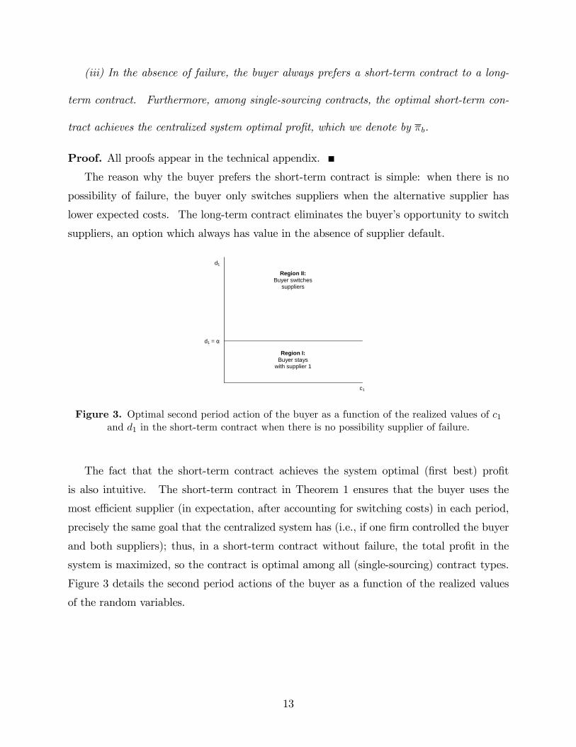
(iii) In the absence of failure, the buyer always prefers a short-term contract to a long-
term contract. Furthermore, among single-sourcing contracts, the optimal short-term con-
tract achieves the centralized system optimal pro�t, which we denote by �b.
Proof. All proofs appear in the technical appendix.
The reason why the buyer prefers the short-term contract is simple: when there is no
possibility of failure, the buyer only switches suppliers when the alternative supplier has
lower expected costs. The long-term contract eliminates the buyer�s opportunity to switch
suppliers, an option which always has value in the absence of supplier default.
c1
d1
Region I:Buyer stays
with supplier 1
Region II:Buyer switches
suppliers
d1 = α
Figure 3. Optimal second period action of the buyer as a function of the realized values of c1and d1 in the short-term contract when there is no possibility supplier of failure.
The fact that the short-term contract achieves the system optimal (�rst best) pro�t
is also intuitive. The short-term contract in Theorem 1 ensures that the buyer uses the
most e¢ cient supplier (in expectation, after accounting for switching costs) in each period,
precisely the same goal that the centralized system has (i.e., if one �rm controlled the buyer
and both suppliers); thus, in a short-term contract without failure, the total pro�t in the
system is maximized, so the contract is optimal among all (single-sourcing) contract types.
Figure 3 details the second period actions of the buyer as a function of the realized values
of the random variables.
13
5. Suppliers Prone to Default
In this section we consider contracts between a buyer and suppliers that are prone to default.
Recall that suppliers default if, at the end of any period, their total pro�t is negative. For
the purposes of the buyer, default only matters if it happens at the end of period 1, i.e., if
p11 < c1 + d1; otherwise, supplier 1 survives.
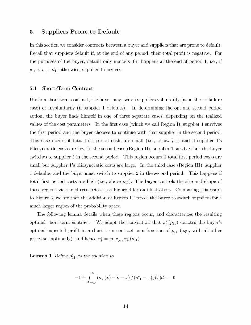
5.1 Short-Term Contract
Under a short-term contract, the buyer may switch suppliers voluntarily (as in the no failure
case) or involuntarily (if supplier 1 defaults). In determining the optimal second period
action, the buyer �nds himself in one of three separate cases, depending on the realized
values of the cost parameters. In the �rst case (which we call Region I), supplier 1 survives
the �rst period and the buyer chooses to continue with that supplier in the second period.
This case occurs if total �rst period costs are small (i.e., below p11) and if supplier 1�s
idiosyncratic costs are low. In the second case (Region II), supplier 1 survives but the buyer
switches to supplier 2 in the second period. This region occurs if total �rst period costs are
small but supplier 1�s idiosyncratic costs are large. In the third case (Region III), supplier
1 defaults, and the buyer must switch to supplier 2 in the second period. This happens if
total �rst period costs are high (i.e., above p11). The buyer controls the size and shape of
these regions via the o¤ered prices; see Figure 4 for an illustration. Comparing this graph
to Figure 3, we see that the addition of Region III forces the buyer to switch suppliers for a
much larger region of the probability space.
The following lemma details when these regions occur, and characterizes the resulting
optimal short-term contract. We adopt the convention that �sb (p11) denotes the buyer�s
optimal expected pro�t in a short-term contract as a function of p11 (e.g., with all other
prices set optimally), and hence �sb = maxp11 �sb (p11).
Lemma 1 De�ne p�11 as the solution to
�1 +Z �
�1(�d (x) + k � x) f(p�11 � x)g(x)dx = 0:
14
Region III:Supplier 1 fails
c1
d1p11 = c1 + d1
Region I:Buyer stays
with supplier 1
Region II:Buyer switches
suppliers
d1 = α
Figure 4. Optimal second period action of the buyer as a function of the realized values of c1and d1 in the short-term contract when there is a risk of supplier failure.
Then the buyer�s optimal short-term contract consists of ps12 = d1 + �2 (c1), ps22 = �d (d1) +
�2 (c1), and
ps11 =
8>><>>:p�11 if p�11 � �d + �c and �sb (p�11) � �sb (�d + �c)
�d + �1 otherwise
;
where �sb (p11) is given by,
�sb (p11) = 2s� p11 � �2 � Pr (c1 + d1 > p11)� E (�d (x) + k jc1 + d1 > p11 ) (3)
�Pr (c1 + d1 � p11)� E (min (d1; �d (x) + k) jc1 + d1 � p11 ) :
The buyer switches suppliers in period 2 if k + �d (d1) < d1.
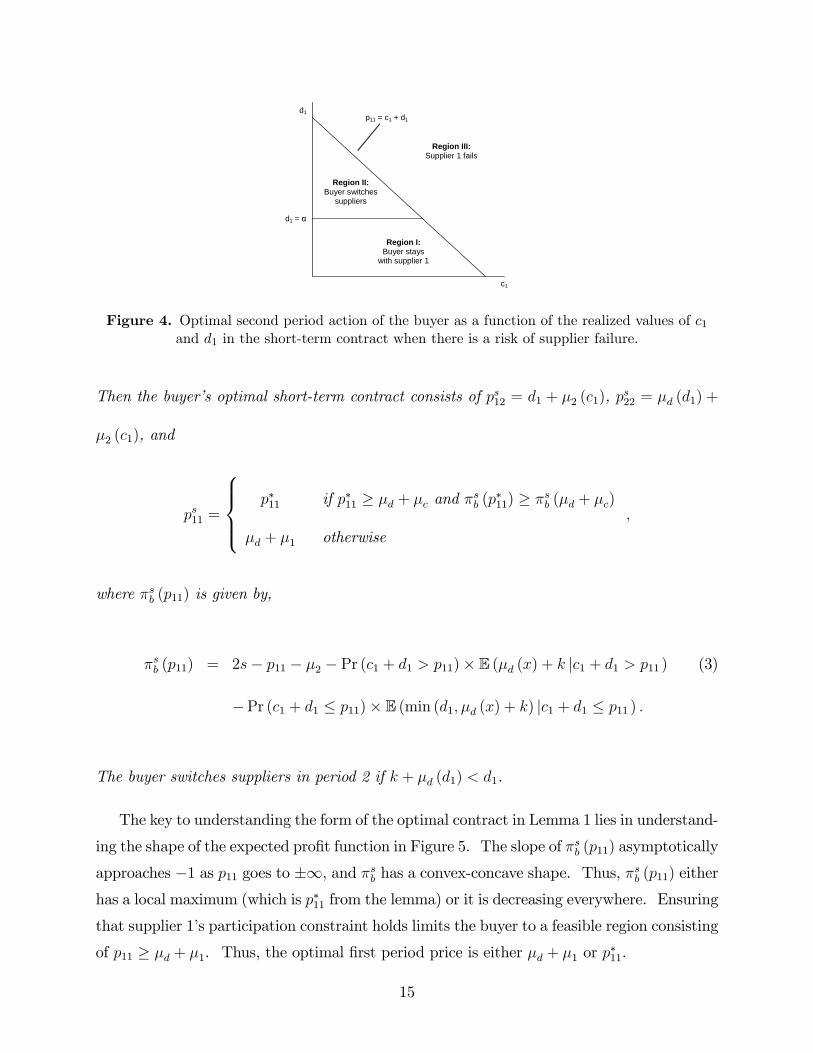
The key to understanding the form of the optimal contract in Lemma 1 lies in understand-
ing the shape of the expected pro�t function in Figure 5. The slope of �sb (p11) asymptotically
approaches �1 as p11 goes to �1, and �sb has a convex-concave shape. Thus, �sb (p11) eitherhas a local maximum (which is p�11 from the lemma) or it is decreasing everywhere. Ensuring
that supplier 1�s participation constraint holds limits the buyer to a feasible region consisting
of p11 � �d + �1. Thus, the optimal �rst period price is either �d + �1 or p�11.
15
Feasible Region
p11
πbs
p11*μd + μ1
Figure 5. An example of the buyer�s expected pro�t as a function of p11 in the single periodcontract with the risk of failure.
The intuition behind this result is that, if switching costs are small, the buyer�s pro�t
is likely to be decreasing in p11; there is little consequence to failure, hence the buyer o¤ers
the lowest possible price. However, if switching costs are high, �sb (p11) has a shape like
that depicted in Figure 5. If p11 is very small, increasing it slightly does nothing to lower
the chance of default and only costs the buyer more; likewise, if p11 is very large, then a
slight increase does little to a¤ect the probability of default. However, if p11 is intermediate
in value then a small change may result in a large decrease in the probability of failure,
outweighing the excess cost to the buyer. Thus, it may be optimal to o¤er a price that
is higher than the supplier�s minimum acceptable price in order to lower the probability of
default.
It is interesting that the optimal contract derived in Lemma 1 is identical to the optimal
contract in Theorem 1, except for the �rst period price ps11, because failure is irrelevant (from
the buyer�s point of view) in the second period. Furthermore, with failure, the �rst period
price is greater than the �rst period price without failure, since the minimum possible price
from Lemma 1 is equal to the optimal price in Theorem 1. Thus, comparing short-term
contracts, we see that the buyer pays more when suppliers face an endogenous default risk
than when suppliers have no risk of default, in order to reduce the probability of failure and
hence the chance of incurring the switching cost k. In addition, by applying the Envelope
Theorem, it can be shown that the buyer�s optimal pro�t is decreasing in k; intuitively, the
more expensive it is to switch suppliers in the middle of the product�s sale horizon, the lower
the buyer�s expected pro�t.
16
Region I:Supplier 1 survives
Region III:Supplier 1 fails
c1
d1p11 = c1 + d1
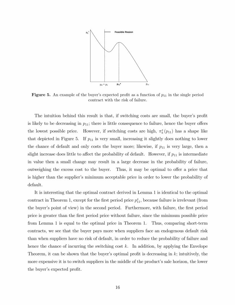
Figure 6. Optimal second period action of the buyer as a function of the realized values of c1and d1 under the long-term contract.
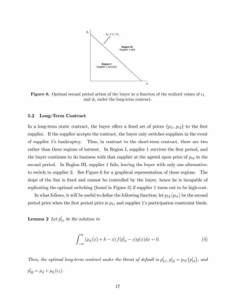
5.2 Long-Term Contract
In a long-term static contract, the buyer o¤ers a �xed set of prices fp11; p12g to the �rstsupplier. If the supplier accepts the contract, the buyer only switches suppliers in the event
of supplier 1�s bankruptcy. Thus, in contrast to the short-term contract, there are two
rather than three regions of interest. In Region I, supplier 1 survives the �rst period, and
the buyer continues to do business with that supplier at the agreed upon price of p12 in the
second period. In Region III, supplier 1 fails, leaving the buyer with only one alternative:
to switch to supplier 2. See Figure 6 for a graphical representation of these regions. The
slope of the line is �xed and cannot be controlled by the buyer, hence he is incapable of
replicating the optimal switching (found in Figure 3) if supplier 1 turns out to be high-cost.
In what follows, it will be useful to de�ne the following function: let p12 (p11) be the second
period price when the �rst period price is p11 and supplier 1�s participation constraint binds.
Lemma 2 Let pl11 be the solution to
Z 1
�1(�d (x) + k � x) f(pl11 � x)g(x)dx = 0: (4)
Then, the optimal long-term contract under the threat of default is pl11, pl12 = p12
�pl11�, and
pl22 = �d + �2 (c1).
17
Note that in Lemma 2, we have not restricted pl12 to be non-negative. Numerically, it
is rare to observe pl12 < 0, but not impossible. For this to occur, the switching cost must
be very large (e.g., an order of magnitude greater than the average total production cost).
The economic interpretation of a negative second period price is that, if the expected cost
incurred due to default is extremely large (i.e., if the chance of default is high or k is large),
it is optimal for the buyer to heavily subsidize the supplier, and in return, if costs turn out to
be low, the supplier reimburses the buyer in the second period for insuring the �rm against
default.
5.3 Contract Choice
To determine which contract the buyer prefers, we must compare expected pro�ts under the
optimal contract in each case.
Theorem 2 In the presence of failure risk, (i) �sb; �lb � �b and (ii) there exists some k� such
that, for all k > k�, �sb � �lb.
In other words, the long-term contract is preferred to the short-term contract if switching
costs are high, but neither contract achieves the system optimal pro�t �b. The �rst part
of theorem is intuitive, as we expect the system to perform no better under the threat of
default than a system without failure. The second part of theorem demonstrates that long-
term contracts are preferred when switching costs are high. Essentially, long-term contracts
allow the buyer to shift more of the total compensation to the �rst period, thus lowering
the chance of supplier failure. This comes at the expense of losing the option to voluntarily
switch suppliers, and hence the buyer only prefers the long-term contract if the savings due
to the decreased chance of default outweigh the lost option to switch suppliers. Numerically,
we observe that the threshold k� is typically very small in relation to the average production
costs in the system (e.g., an order of magnitude or more), and in many cases the long-term
contract is preferred for all non-negative values of k. In a numerical study consisting of 243
sets of parameters (see §5 of the appendix for details), we found that on average, k� was
27% of the total mean per unit production cost. Thus, for many reasonable parameters
(i.e., moderately signi�cant switching costs satisfying k & 0:3 (�c + �1)), the buyer prefers
the long-term contract.
18
0 2 4
Coefficient of Variation of Idiosyncratic Costs (di)Th
resh
old
Sw
itchi
ng C
ost (
k*)
ρd = 0.5
ρd = 0
ρd = 0.5
2
1
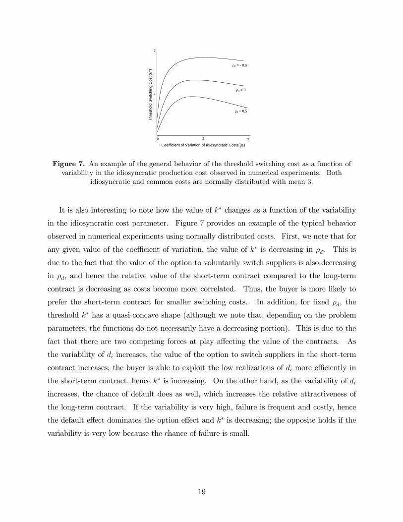
Figure 7. An example of the general behavior of the threshold switching cost as a function ofvariability in the idiosyncratic production cost observed in numerical experiments. Both
idiosyncratic and common costs are normally distributed with mean 3.
It is also interesting to note how the value of k� changes as a function of the variability
in the idiosyncratic cost parameter. Figure 7 provides an example of the typical behavior
observed in numerical experiments using normally distributed costs. First, we note that for
any given value of the coe¢ cient of variation, the value of k� is decreasing in �d. This is
due to the fact that the value of the option to voluntarily switch suppliers is also decreasing
in �d, and hence the relative value of the short-term contract compared to the long-term
contract is decreasing as costs become more correlated. Thus, the buyer is more likely to
prefer the short-term contract for smaller switching costs. In addition, for �xed �d, the
threshold k� has a quasi-concave shape (although we note that, depending on the problem
parameters, the functions do not necessarily have a decreasing portion). This is due to the
fact that there are two competing forces at play a¤ecting the value of the contracts. As
the variability of di increases, the value of the option to switch suppliers in the short-term
contract increases; the buyer is able to exploit the low realizations of di more e¢ ciently in
the short-term contract, hence k� is increasing. On the other hand, as the variability of di
increases, the chance of default does as well, which increases the relative attractiveness of
the long-term contract. If the variability is very high, failure is frequent and costly, hence
the default e¤ect dominates the option e¤ect and k� is decreasing; the opposite holds if the
variability is very low because the chance of failure is small.
19
6. Dynamic Contracts
Now that we have shown that the contracts described in the previous sections perform
worse than the centralized system, we move on to a class of contracts that does coordinate
the channel. This class of contracts is �dynamic� or state-dependent, as opposed to the
previous �static� contracts. The sequence of events is precisely the same in a dynamic
contract as in a static contract. The di¤erence between the two is that the prices in a static
contract are �xed, whereas prices in a dynamic contract may be tied to some index in order
to help insulate the supplier against failure by shifting some of the risk to the buyer. For
example, suppose the uncertainty in the common cost ct is primarily due to �uctuations in
the global petroleum market. Then in forming a dynamic contract, the buyer might tie
the contract price to the commodity price of oil, compensating the supplier for part or all
of the variation in the common cost. These types of contracts are frequently observed in
Japanese industry, contrasting with traditionally static contracts in the U.S. industry. For
example, McMillan (1990) describes how Japanese manufacturers typically do not specify
prices in initial contracts, but rather update prices every six months based on a review of
the supplier�s production costs, considering separately such issues as labor, raw materials,
design changes and energy costs. Buyers typically allow unavoidable cost increases, such as
raw materials, to be re�ected in the contract price, but are less likely to allow increases due
to controllable costs, such as labor.
For the purpose of our analysis, we assume that the dynamic contract compensates the
supplier perfectly for ct. E¤ectively, this assumption removes ct from the contracting problem
by having the buyer bear this cost in its entirety. The decision of the buyer is then how
to compensate the supplier for idiosyncratic costs, di. Since this contract will be shown to
coordinate the channel, there is no loss of generality in restricting attention to this particular
form of cost compensation as opposed to some other form (e.g., dynamically compensating
for idiosyncratic costs or some combination of the two components).
We assume that there is no additional cost to implementing a dynamic contract; however,
dynamic contracts may indeed be di¢ cult or costly to administer, factors which may reduce
their relative attractiveness. Administrative costs are not explicitly modeled here, but
might include, for example, tracking and veri�cation of the pricing index which determines
the supplier�s compensation.
20
6.1 Dynamic Contracts without Failure
The following lemma details the optimal contracts for the no failure case.
Lemma 3 (i) The optimal short-term dynamic contract is ps11 = �d+ c1, ps12 = d1+ c2, and
ps22 = �d (d1) + c2. The buyer switches suppliers in the second period if k + �d (d1) < d1.
(ii) The optimal long-term dynamic contract is any pair fpl11; pl12g such that pl11 + pl12 =
2�d + �1 + �2.
(iii) The expected pro�t in each dynamic contract is equal to the expected pro�t in their
static counterparts in Theorem 1.
The preceding lemma provides an interesting result: in the absence of failure risk, in
terms of expected pro�t, the dynamic contracts are equivalent to static contracts of the
same length. In other words, to a risk neutral buyer, choosing a dynamic contract o¤ers no
advantage.
6.2 Dynamic Contracts with Failure
Dynamic contracts transfer the risk of common cost uncertainty from the supplier to the
buyer, thus lowering the probability of failure due to high common costs. Since we assume
that the buyer is a large, risk-neutral �rm, transferring this risk increases the relative attrac-
tiveness of the dynamic contracts to the buyer when supplier failure is a possibility. The
following lemma demonstrates this fact.
Lemma 4 (i) The optimal long-term dynamic contract is pl11 = �+ c1, pl12 = p12
�pl11�, and
pl22 = �d (d1) + c2, where p12(pl11) is the dynamic second period price for which the supplier�s
participation constraint binds.
(ii) The optimal short-term dynamic contract is given by ps11 = c1 + max (x�; �d), p
s12 =
21
d1 + c2, and ps22 = �d (d1) + c2, where x� is the solution to
�1 + g(x�) (�x� + �d (x�) + k) = 0:
(iii) The long-term dynamic contract is preferred to the short-term dynamic contract, and
yields expected pro�t equal to the system optimal expected pro�t without failure risk.
It is interesting that in Lemma 4 we have precisely the opposite result from Theorem 1:
long-term dynamic contracts are always preferred to short-term dynamic contracts. The
reason is that long-term contracts allow the buyer to switch suppliers in the optimal manner;
by setting p11 = �+c1, supplier 1 fails (and hence the buyer switches suppliers) if �d(d1)+k <
d1, exactly the same action the centralized system would make. The second period price
then serves as a compensation mechanism to ensure supplier 1 has a binding participation
constraint. In the short-term contract, however, second period prices must be subgame
perfect. Thus, the buyer cannot promise a price that justi�es setting p11 = � + c1 as
the �rst period price, and hence he cannot switch suppliers in the system optimal manner.
Consequently, the �rst period price is strictly less than � + c1 and total pro�ts are lower
than in the long-term contract.
The fact that long-term dynamic contracts in the presence of default risk achieve the sys-
tem optimal solution without failure is intriguing. It means that buyers can simultaneously
lock-in suppliers, form lasting relationships built on trust and dynamic cost compensation,
yet still achieve the proper �ltering of costly suppliers in order to maximize their own pro�ts.
Indeed, if we were to plot the actions resulting from the optimal dynamic long-term contract
it would look exactly like Figure 3, with the only di¤erence being that the regions in the
dynamic contract case are determined by failure rather than by the buyer�s choice to switch
suppliers. Furthermore, since a �rst period price of �+c1 is never optimal in the short-term
dynamic contract, this contract is incapable of replicating the switching in Figure 3 and
hence cannot coordinate the channel.
The value of a dynamic contract lies in its ability to remove the stochastic element that
a¤ects both suppliers from the factors a¤ecting default. With static contracts, a potentially
e¢ cient supplier (i.e., a supplier with lower idiosyncratic costs than the expected costs of the
alternative supplier) may fail due to high common costs, which reduces overall supply chain
22
e¢ ciency; with dynamic contracts, on the other hand, suppliers only fail if their idiosyncratic
costs are high, precisely the situation in which the buyer would switch suppliers voluntarily.
Hence, dynamic contracts eliminate a harmful source of stochasticity (common costs) while
retaining a potentially useful source of stochasticity (idiosyncratic costs), from the supply
chain�s point of view.
7. Extensions
In this section we analyze four independent extensions to the core model that allow us to
comment further on the scope of our results. In the �rst subsection we consider the e¤ects
of demand uncertainty. The second subsection addresses contingent transfer payments�
that is, transfer payments made from the buyer to a supplier (possibly dependent on cost
realizations) intended to subsidize the supplier and prevent bankruptcy. The third subsec-
tion addresses the issue of renegotiation. The �nal subsection discusses the special case
of normally distributed costs, using the increased speci�city of the model to answer several
interesting questions concerning the performance of the various contracts as a function of
cost correlation and uncertainty.
7.1 Demand Uncertainty
We have assumed throughout the paper that the buyer�s demand is deterministic and equal
to one in each period. In practice, suppliers may face demand uncertainty in addition to
cost uncertainty. However, because we have explicitly incorporated cost uncertainty into
the model, this assumption is equivalent to a make-to-order system with uncertain demand.
To see this, consider a supplier that only produces units that are purchased by the buyer.
The total size of the buyer�s order in period t is a random variable Dt that is independent
of both idiosyncratic costs, di, and common costs, ct. The supplier may face exogenous
capacity constraints, in which case Dt is truncated at the capacity level of the supplier with
mass added to the endpoint. The pro�t to supplier i in period t is then Dt (pt � di � ct).Assume that the supplier must make a minimum pro�t of Kt in period t in order to
survive. Kt may represent the supplier�s annual (�xed) operating costs, interest payments
on outstanding loans, capital outlay for the new production process, legacy pension expenses,
etc. Note that Kt is allowed to be negative, i.e., the supplier may be allowed to lose some
23
money and still survive, and may evolve across time; however, because suppliers are ex-ante
identical, Kt is the same for both suppliers in each period. Thus, supplier i survives in
period t if Dt(pt � di � ct) � Kt. Since all the random variables are independent from
one another, we may write this as pt � di � ct � Kt=Dt. Rede�ning the common cost to
incorporate the demand term, c0t = ct +Kt=Dt, we see that supplier i survives if and only if
pro�t is non-negative, i.e.,
pt � di � c0t � 0: (5)
In addition, we may consider the case in which the supplier only accepts a contract that
yields expected pro�ts of at least Kt. In that case, the same logic yields the result that the
supplier accepts any contract in which (5) holds in expectation. Both of these conditions�
supplier survival and contract acceptance�are identical to the case with deterministic demand
in each period, so long as the common cost terms are properly de�ned; consequently, our
assumptions of deterministic demand and no �xed operating expenses are made without loss
of generality in a make-to-order production system with exogenous capacity constraints.
This equivalence also yields insight into why the common cost term is not diversi�able
and hence cannot be hedged; because the common cost term may be thought of as capturing
demand risk as well as common cost risk, it is unlikely that this risk could be mitigated.
Furthermore, because the cost term also depends on materials prices that cannot be pro-
cured from any industrial exchange (e.g., the outputs of upstream suppliers), our implicit
assumption that cost uncertainty cannot be hedged is justi�ed.
It is important to note that our extension to the case of demand uncertainty is only valid
if the supplier is uncapacitated or faces an exogenous capacity constraint. This scenario is
re�ective of our motivating example (the auto industry) in which the capacity is sometimes
dictated by the buyer, suppliers may not have su¢ cient capital for creating excess capacity,
capacity constraints on components are typically not tight (i.e., it is more likely that assembly
capacity is binding) and, if capacity is likely to be tight, components are multi-sourced. By
focusing on a single-sourced component, we have implicitly assumed that capacity constraints
are not an issue for the supplier; a model in which capacity is tight may be more suitable to an
analysis of multi-sourcing, see Tomlin (2006). In any event, endogenous capacity decisions
are likely to provide further reasons to favor long-term contracts, as long-term relationships
are known to stimulate capacity investment (Taylor and Plambeck 2003), hence it is unlikely
that endogenizing the capacity decision would signi�cantly alter our results.
24
7.2 Contingent Transfer Payments and Loans
The contract types we have discussed thus far are fairly simple, consisting of either �xed
prices or prices that are a function of one of the stochastic elements (i.e., the common cost).
When a supplier enters bankruptcy, we provide no recourse to the buyer to help alleviate
the supplier�s �nancial distress. This may be an acceptable assumption if the buyer is
unable or unwilling to subsidize the supplier in the event of bankruptcy (e.g., if capital
is expensive to the buyer, or if the buyer is also in �nancial distress); however, in some
situations the buyer may prefer to make a transfer payment that allows the supplier to avoid
bankruptcy and continue operations with the buyer. For example, the Big Three Detroit
automakers provided $100 million in direct operating subsidies to support Collins & Aikman
in bankruptcy in 2006 (Barkholz and Sherefkin 2007). In this section, we discuss precisely
this scenario.
We consider the following modi�cation of the core model: if the �rst supplier enters
bankruptcy, then at the start of the second period, upon observing the realized value of all
costs, the buyer has the option of either switching suppliers or making a transfer payment to
the �rst supplier that raises the capital level to zero and prevents bankruptcy. In making this
decision, the buyer takes into account the size of the necessary transfer payment as well as
the costs of contracting with each supplier and any switching costs. The resulting transfer
payment thus depends upon the realized value of both �rst period cost terms, hence it is
termed a contingent transfer payment. In addition to allowing direct operating subsidies
that are not reimbursed, we also consider loans from the buyer to the supplier that may
be partially for fully repaid (with interest). We refer to either scenario (no repayment, or
repayment) as a transfer payment.
For the details of our model of transfer payments, we refer the reader to §2 of the technical
appendix. We state here, however, a critical assumption concerning the timing of the
transfer payment. In what follows, we assume any transfer payment occurs at the start
of the second period, and that such payments are not considered in the short-term (i.e.,
one period) participation constraint of the supplier. The implication of this assumption
is that the supplier is unwilling to accept a lower �rst period price if the buyer has the
option of o¤ering a transfer payment when bankruptcy occurs. The short-term participation
constraint represents the outside option of the supplier over the immediate future; given the
�nancial distress of the �rm, the primary concern (particularly when engaging in a short-term
25
contract without the promise of future business) is likely short-term �nancial performance,
and hence the supplier is likely unwilling to sacri�ce short-term pro�t for a potential future
transfer payment, especially when this may greatly increase the chance of bankruptcy. The
consequences of this assumption are discussed in more detail below.
It is clear that the buyer does at least as well when allowed to make a transfer payment as
he does in the simpler contracts we have discussed previously, since the transfer payment is
entirely optional. Thus, contracts with transfer payments are preferred to contracts without
such payments. The questions we then seek to address are the following. Firstly, does the
result of Theorem 2 hold with transfer payments? In other words, are long-term contracts
preferred when switching costs are high, even if transfer payments are available under both
short- and long-term contract types? Secondly, does either contract type coordinate the
system (i.e., achieve the �rst-best solution that the long-term dynamic contract without
transfer payments achieves)?
The following theorem answers both of the questions, essentially demonstrating that all
of the results of Theorem 2 hold even when the buyer is given the option of subsidizing
distressed suppliers.
Theorem 3 If the buyer is allowed to make contingent transfer payments or loans, then
(i) neither the short-term nor the long-term contract achieves the �rst best pro�t (�b) and
(ii) there exists some k� such that, for all k > k�, the long-term contract is preferred to the
short-term contract.
The intuition behind this result is that transfer payments and loans allow the buyer to
avoid switching suppliers in the event of failure, provided the incumbent supplier is e¢ cient
enough to warrant a subsidy. However, this bene�t of transfer payments applies to both
short- and long-term contracts in di¤erent ways. Transfer payments are valuable with
short-term contracts because these contracts typically involve lower �rst period prices and
higher failure rates than long-term contracts, hence the recourse provided in subsidizing a
bankrupt supplier is greater with short-term contracts because failure happens more often.
On the other hand, transfer payments introduce an option to stay with an e¢ cient (albeit
bankrupt) supplier in long-term contracts, hence there is an increase in value due to the
second period option e¤ect. Numerically, we observe that neither bene�t dominates, and
26
the e¤ect on k� (compared to the case of no transfer payments) is ambiguous: in a numerical
study consisting of 243 sets of parameters (see §5 of the appendix for details), we found
that on average, k� was 18% of the total mean per unit production cost, compared to 27%
without transfer payments. In 42 out 243 cases, k� increased due to the presence of transfer
payments (i.e., the transfer payment provided more value to the short-term contract than
to the long-term contract), while in the remaining 201 cases, k� was lower with a transfer
payment.
Recall that we assumed that any transfer payment is made at the start of the second
period (or, more importantly, that the supplier does not consider the transfer payment in
his short-term contract participation constraint). This is a key assumption: if the supplier
does take the transfer payment into account, for large k the short-term contract essentially
transforms into a long-term contract in the following sense. If switching costs are high,
the buyer pays the supplier nothing for �rst period production. Consequently, the supplier
always fails. The buyer never switches suppliers, however, preferring instead to make a
transfer payment to the bankrupt supplier and avoid high switching costs. The short-term
contract has e¤ectively become a long-term contract in which the buyer promises to work
with supplier 1 in the second period and pay all production costs ex-post after the supplier
enters bankruptcy, and as a result the expected pro�t is the same with a long-term and
short-term contract as k becomes large, hence there is not a strict preference between the
two. (For low switching costs, as in all other cases we have considered, it remains true that
the short-term contract is preferred to the long-term contract.)
This equivalence is eliminated and a strict preference for long-term contracts is restored
if any of several complications arise, including: if the supplier is unwilling to accept certain
bankruptcy (because of a contract price of zero) in the �rst period, i.e., there is a minimum
acceptable contract price; if there is some �xed cost to making a transfer payment (e.g., the
buyer must pay the supplier�s bankruptcy or default penalty); or if the supplier discounts
future revenues (which implies the supplier will not accept a contract price of zero even if a
transfer payment is made in the future). Thus, although the timing of the transfer payment
is important to the result of Theorem 3, this assumption may be relaxed while preserving
the result if a one of a variety of alternative conditions holds.
While we have assumed that the suppliers in the current analysis are incapable of securing
external funds in the event of bankruptcy between periods one and two, it is interesting to
consider this case. If the supplier is capable of borrowing enough funds in any scenario to
27
avert bankruptcy, then clearly failure has no e¤ect to the buyer; the supplier always avoids
bankruptcy and hence the model is equivalent to the model without default. If the supplier
is capable of borrowing limited funds, however, and the chance of default remains, then the
core results of the model are preserved; it is still true that long-term contracts hold value in
allowing the buyer to rearrange the cash �ows and helping the supplier avoid default.
7.3 Renegotiation
We explicitly excluded the possibility of supplier renegotiation (i.e., supplier hold-up) in
long-term contracts due to the strong bargaining power of the buyer. However, there
is a possibility of buyer initiated renegotiation, as in the Ford example discussed in the
introduction. It is possible to show (see §3 of the technical appendix) that, if the buyer
is allowed to renegotiate a long-term contract in the second period, all of the results are
preserved. This result critically depends on the fact that, with or without renegotiation,
the supplier�s participation constraint is binding in the optimal contract. Thus, the buyer
extracts all surplus from the supplier, and if renegotiation occurs (and the supplier anticipates
the renegotiation) the buyer must compensate the supplier via a higher �rst period price to
satisfy the supplier�s participation constraint. In other words, any additional dollar extracted
via renegotiation must be compensated for via the contract price. The net result is that
the buyer�s expected pro�t is the same regardless of whether renegotiation occurs, hence the
preference between contracts remains identical to the cases already discussed in §§3�6.
Interestingly, if the supplier does not anticipate renegotiation in a long-term contract
(i.e., if renegotiation is not taken into account in the supplier�s participation constraint),
then the buyer enjoys strictly greater pro�ts in a long-term contract than in a model without
renegotiation because the buyer need not compensate the supplier with a higher contract
price. As a result, long-term contracts have even greater value than previously discussed,
and they are thus preferred for large switching costs. Hence, the results of the paper hold
even when the buyer is allowed to unilaterally renegotiate in long-term contracts, regardless
of whether the supplier anticipates that the contract will be renegotiated.
28
7.4 Normally Distributed Costs
By assuming that costs are normally distributed, we are able to derive further insights
into the behavior of the various contracts. In what follows we consider three contract
types in the presence of default risk: the long-term static and dynamic contracts and the
short-term static contract. Since the long-term dynamic contract dominates the short-
term dynamic contract, the latter case is uninteresting and is hence omitted. Let c1; c2 be
identically distributed (possibly correlated) N (�c; �c) random variables, and let d1; d2 be
bivariate normal with identical mean and variance �d and �2d, and correlation �d. From
the properties of the bivariate normal distribution, the expected value of d2 conditional on
d1 = x is �d (x) = (1� �d)�d + �dx. Hence, it is optimal to switch suppliers in the secondperiod if d1 > �d + k= (1� �d). Since � is increasing in �d, it is apparent that the buyer isless likely to switch suppliers if costs are highly correlated. The following theorem further
describes the behavior of the contracts as a function of �d and �d.
Theorem 4 (i) The optimal expected pro�t under all contract types is decreasing in �d.
(ii) The di¤erence between the system optimal (long-term dynamic) pro�t and the pro�t
under the long-term static contract is decreasing in �d. In the limit as �d ! 1, pro�ts are
equal.
(iii) The centralized system optimal expected pro�t is increasing in �d.
Intuitively, from part (i), the pro�t of the system is lower if the idiosyncratic costs of
the two �rms are highly correlated; there is little value contained in the option to switch
suppliers, so the overall expected pro�t of the buyer is higher when suppliers have negatively
correlated idiosyncratic costs.
Part (ii) demonstrates how the relative advantage of the dynamic long-term contract
varies as a function of �d. If costs are strongly negatively correlated, then the dynamic
long-term contract performs quite well; in this case, the dynamic contract is e¤ective at
switching suppliers in the optimal manner, while the static contract is less e¢ cient. If costs
are strongly positively correlated, however, the value of switching suppliers is lower, hence
the performance gap between the two contract types is much smaller, although dynamic
29
contracts o¤er value for any �d < 1. Consequently, long-term dynamic contracts are most
valuable in situations wherein suppliers have negatively correlated costs.
Part (iii) describes the behavior of the system optimal expected pro�t as a function
of variability in the suppliers� private cost. Intuitively, the more variable the costs of
the suppliers, the more likely a low cost realization is; the buyer is shielded from high cost
realizations by the option to switch suppliers. Thus, for �xed �d and �d, increased variability
in the idiosyncratic costs of the suppliers allows the buyer to exploit his option to switch.
8. Discussion
In this paper, we have presented a model of buyer-supplier contracting primarily character-
ized by three features: uncertain production costs, extended sales horizons, and the strong
bargaining power of the buyer. Within this context, we have shown that the threat of
supplier failure can increase the buyer�s preference for long-term contracts. Furthermore,
dynamic contracts which compensate the suppliers for common costs (materials, etc.) achieve
the system optimal pro�t. This feature helps to explain the adoption of these contracts in
the Japanese auto industry (McMillan 1990).
We did not model risk-averse �rms because discussing supply chain coordination in such
a setting adds another level of complexity that is outside the scope of our work (Gan et al.
2004). However, the true value of dynamic contracts may depend on the risk-neutrality
(or lack thereof) of the buyer. In practice, auto manufacturers do not always reimburse
suppliers for the full amount of common costs; one potential explanation for this behavior is
that the buyer is not risk-neutral, and hence does not seek to bear all of the risk associated
with the variability in raw materials costs. Another possible explanation may be that the
variability associated with ct is not completely outside of the supplier�s control, hence the
buyer needs to leave some of the risk with the supplier in order to induce the proper actions
(e.g., negotiating low prices from second tier suppliers, etc.). Finally (and perhaps most
importantly), dynamic contracts are di¢ cult to administer and are signi�cantly less formal
than static contracts, and trust between partners is key to their implementation. There
has historically been a severe lack of trust between U.S. auto manufacturers and suppliers,
perhaps helping to explain why both parties are hesitant to engage in dynamic contracting
agreements.
30
Throughout the analysis, we have ignored the e¤ects of learning curves, seen for example
in Spence (1981). In much of the multiperiod contracting literature, learning curves are
modeled as cooperative improvements in design and production processes that reduce costs
in long-term relationships (e.g., Cohen and Agrawal 1999), whereas short-term relationships
o¤er lesser (or no) opportunities for cost reduction. If such a learning curve were present
in our model, it would serve to increase the pro�tability of the long-term contract, thus
providing further incentive for a buyer to choose this contract type. Qualitatively, our main
results should be strengthened by this complication. In addition, considering asymmetric
suppliers yields a similar result: if one supplier�s costs dominate the other supplier, the
buyer will seek to contract in the �rst period with the more e¢ cient supplier. The long-
term contract then serves as a tool to both mitigate switching costs and prevent switching
to a less e¢ cient supplier; thus, the value of the long-term contract is increased.
An interesting counterpart to the case of contingent transfer payments are contracts that
explicitly allow the buyer to end the relationship should the production costs of the supplier
exceed a certain threshold (i.e., the buyer is provided a means of breaking the relationship if
a supplier is very ine¢ cient). Such a contract, which would provide the buyer the option of
switching suppliers if the �rst supplier survives (rather than fails) increases the pro�tability
of long-term relationships and hence increases the relative attractiveness of a long-term
contract compared to a short-term contract, leaving our main results intact. Such contracts
are unable to coordinate the system, however, because of the forced switching of suppliers
that occurs if the incumbent supplier fails. Thus, dynamic contracts still perform better by
achieving coordination.
There are two complications that may increase the relative value of short-term contracts:
discounting of the buyer�s second period pro�t, and non-zero bankruptcy costs for the sup-
pliers. The �rst complication lessens the impact of supplier default and the cost of voluntary
switching: since both of these costs are incurred in the second period, discounting decreases
their relative contribution to the total expected pro�t. The second complication e¤ectively
increases the switching costs due to default, while leaving unchanged the switching costs due
to voluntary changes in the second period supplier. Intuitively, if the suppliers incur some
bankruptcy penalty, the buyer must compensate the supplier more in order to satisfy the
participation constraint; thus, if the participation constraint is binding, the buyer�s pro�t
function includes an extra term penalizing for the bankruptcy costs if default occurs, which
is essentially the same as increasing the switching cost k. The extra term is not present,
31
however, when the supplier survives but the buyer voluntarily switches suppliers, hence the
relative value of the short-term contract is increased because voluntary switching is less
costly. Both of these complications essentially increase the threshold k� from Theorem 2,
but other results remain qualitatively unchanged.
Our model is one of partial equilibrium; in reality, as distressed suppliers enter bankruptcy
and exit the market, new suppliers may enter, perhaps in better �nancial standing. This
e¤ect is important in the automotive industry, but occurs over long time scales (e.g., it may
take years for a newly created supplier to build the necessary technology to produce at the
scale and quality level of a large, existing supplier such as Delphi). Our model analyzes the
medium-term issue of dealing with a distressed supplier base. In this time frame, it is often
impractical for a buyer to work with an emerging supplier: particularly in the automotive
industry, asset speci�c investments in suppliers are quite large and hence switching costs are
prohibitive.
With no information asymmetry for suppliers to use as leverage, we have created a
situation wherein buyers extract all of the surplus in the supply chain. This assumption
has provided the strongest incentive for the buyer to engage in a short-term contract in
order to exploit the option to voluntarily switch suppliers, and still we �nd that long-term
commitment is very often the more pro�table choice; unlike the results in Li and Debo
(2005), the attractiveness of the long-term contract in our model is not driven by increased
price competition in the supplier�s bidding strategies, but rather by the decreased chance of
failure resulting from a long-term commitment.
The main conclusion of our analysis is that long-term contracts may be even more valu-
able to buyer-supplier relations�particularly within the American automotive industry�than
previously thought. The literature abounds with reasons for �rms to prefer long-term con-
tracts: as a manner of developing trust and cooperation between partners (Dyer 1996), as a
tool to increase price competition in auction scenarios (Li and Debo 2005), and as relational
tools to enforce actions which are otherwise unsupportable or uncontractable in short-term
situations (Taylor and Plambeck 2003). We add to those reasons by demonstrating the
value of long-term relationships when suppliers face the threat of failure.
Acknowledgements. The authors are grateful to Vlad Babich, Chris Tang, and to
the associate editor and three anonymous referees for many helpful comments that greatly
improved the paper.
32
References
Andersson, Bo. 2006. GM�s global supply footprint. Presentation, The Supplier Industry inTransition Conference.
Archibald, T. W., L. C. Thomas, J. M. Betts, R. B. Johnston. 2002. Should start-up compa-nies be cautious? Inventory policies which maximise survival probabilities. ManagementScience 48(9) 1161�1174.
Atkins, Derek, Harish Krishnan, Xuan Zhao. 2005. Relational price-only contracts in supplychains. Working paper, University of British Columbia.
Babich, Volodymyr. 2006. Dealing with supplier bankruptcy: Costs and bene�ts of �nancialsubsidies. Working paper, University of Michigan.
Babich, Volodymyr, Apostolos N. Burnetas, Peter H. Ritchken. 2005. Competition anddiversi�cation e¤ects in supply chains with supplier default risk. Working paper, Universityof Michigan.
Barkholz, David, Robert Sherefkin. 2006. Lear left reeling from Dodge Ram snub. Automo-tive News.
Barkholz, David, Robert Sherefkin. 2007. C&A debacle will cost automakers 665 million.Automotive News.
Cachon, Gerard. 2003. Supply chain coordination with contracts. Handbooks in OperationsResearch and Management Science: Supply Chain Management , chap. 6. North Holland.
Choi, Thomas Y., Janet L. Hartley. 1996. An exploration of supplier selection practicesacross the supply chain. Journal of Operations Management 14 333�343.
Cohen, Morris A., Narendra Agrawal. 1999. An analytical comparison of long and shortterm contracts. IIE Transactions 31(8) 783�796.
Dyer, Je¤rey. 1996. How Chrysler created an American keiretsu. Harvard Business Review74(4) 42�56.
Dyer, Je¤rey, Dong Sung Cho, Wujin Chu. 1998. Strategic supplier segmentation: The next�best practice�in supply chain management. California Management Review 40(2) 57�77.
Gan, Xianghua, Suresh P. Sethi, Houmin Yan. 2004. Coordination of supply chains withrisk-averse agents. Production and Operations Management 13(2) 135�149.
Kleindorfer, Paul R., D. J. Wu. 2003. Integrating long- and short-term contractingvia business-to-business exchanges for capital-intensive industries. Management Science49(11) 1597�1615.
Levy, Efraim, Steve Ferazani. 2006. Industry survey: Autos and auto parts. Standard andPoor.
33
Lewin, Tony. 2006. U.S. suppliers count on Europe for rescue. Automotive News.
Li, Cuihong, Laurens Debo. 2005. Strategic dynamic sourcing from competing suppliers:The value of commitment. Working paper, Carnegie Mellon University.
McMillan, John. 1990. Managing suppliers: Incentive systems in Japanese and U.S. inudstry.California Management Review 38�55.
Nussel, Philip, David Barkholz. 2006. Delphi demands price hikes. Automotive News.
Plambeck, Erica, Terry Taylor. 2007. Implications of renegotiation for optimal contract�exibility and investment. Forthcoming, Management Science.
Rudambi, Ram, Susan Helper. 1998. The �close but adversarial �model of supplier relationsin the U.S. auto industry. Strategic Management Journal 19 775�792.
Sako, Mari, Susan Helper. 1998. Determinants of trust in supplier relations: Evidence fromthe automative industry in Japan and the United States. Journal of Economic Behaviorand Organization 34 387�417.
Sherefkin, Robert. 2006. Ford seeks steel futures market. Automotive News.
Spence, A. Michael. 1981. The learning curve and competition. The Bell Journal of Eco-nomics 12(1) 49�70.
Srinivasan, Raji, Thomas H. Brush. 2006. Supplier performance in vertical alliances: thee¤ects of self-enforcing agreements and enforceable contracts. Organization Science 17(4)436�452.
Stallkamp, Thomas T. 2005. Score! A Better Way to Do Business. Wharton School Pub-lishing.
Swinney, Robert, Gerard Cachon, Serguei Netessine. 2005. Capacity investment by compet-itive start-ups. Working paper, University of Pennsylvania.
Tang, Christopher S. 1999. Supplier relationship map. International Journal of Logistics:Research and Applications 2(1) 39�56.
Taylor, Terry, Erica Plambeck. 2003. Supply chain relationships and contracts: The impact ofrepeated interaction on capacity investment and procurement. Forthcoming, ManagementScience.
Tomlin, Brian. 2006. On the value of mitigation and contingency strategies for managingsupply chain disruption risks. Management Science 52(5) 639�657.
Tunca, Tunay I., Stefanos A. Zenios. 2006. Supply auctions and relational contracts forprocurement. Manufacturing & Service Operations Management 8(1) 43�67.
Wernle, Bradford. 2006a. Suppliers in �shambles,�so why�s Ross buying? Automotive News.
34
Wernle, Bradford. 2006b. Toyota: Supplier-automaker ties need shoring up. AutomotiveNews.
Wynn, Gerard. 2006. General Motors woes seen causing supply chain cull. Reuters article.
35
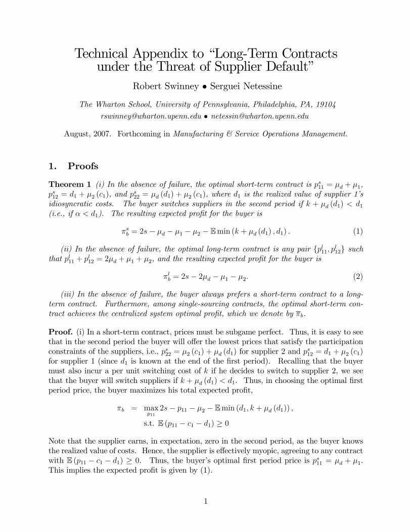
Technical Appendix to �Long-Term Contractsunder the Threat of Supplier Default�
Robert Swinney � Serguei Netessine
The Wharton School, University of Pennsylvania, Philadelphia, PA, 19104
[email protected] � [email protected]
August, 2007. Forthcoming in Manufacturing & Service Operations Management.
1. Proofs
Theorem 1 (i) In the absence of failure, the optimal short-term contract is ps11 = �d + �1,ps12 = d1 + �2 (c1), and p
s22 = �d (d1) + �2 (c1), where d1 is the realized value of supplier 1�s
idiosyncratic costs. The buyer switches suppliers in the second period if k + �d (d1) < d1(i.e., if � < d1). The resulting expected pro�t for the buyer is
�sb = 2s� �d � �1 � �2 � Emin (k + �d (d1) ; d1) : (1)
(ii) In the absence of failure, the optimal long-term contract is any pair fpl11; pl12g suchthat pl11 + p
l12 = 2�d + �1 + �2, and the resulting expected pro�t for the buyer is
�lb = 2s� 2�d � �1 � �2: (2)
(iii) In the absence of failure, the buyer always prefers a short-term contract to a long-term contract. Furthermore, among single-sourcing contracts, the optimal short-term con-tract achieves the centralized system optimal pro�t, which we denote by �b.
Proof. (i) In a short-term contract, prices must be subgame perfect. Thus, it is easy to seethat in the second period the buyer will o¤er the lowest prices that satisfy the participationconstraints of the suppliers, i.e., ps22 = �2 (c1) + �d (d1) for supplier 2 and p
s12 = d1 + �2 (c1)
for supplier 1 (since d1 is known at the end of the �rst period). Recalling that the buyermust also incur a per unit switching cost of k if he decides to switch to supplier 2, we seethat the buyer will switch suppliers if k + �d (d1) < d1. Thus, in choosing the optimal �rstperiod price, the buyer maximizes his total expected pro�t,
�b = maxp11
2s� p11 � �2 � Emin (d1; k + �d (d1)) ;
s.t. E (p11 � c1 � d1) � 0
Note that the supplier earns, in expectation, zero in the second period, as the buyer knowsthe realized value of costs. Hence, the supplier is e¤ectively myopic, agreeing to any contractwith E (p11 � c1 � d1) � 0. Thus, the buyer�s optimal �rst period price is ps11 = �d + �1.This implies the expected pro�t is given by (1).
1
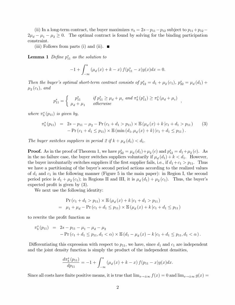
(ii) In a long-term contract, the buyer maximizes �b = 2s�p11�p12 subject to p11+p12�2�d � �1 � �2 � 0. The optimal contract is found by solving for the binding participationconstraint.(iii) Follows from parts (i) and (ii).
Lemma 1 De�ne p�11 as the solution to
�1 +Z �
�1(�d (x) + k � x) f(p�11 � x)g(x)dx = 0:
Then the buyer�s optimal short-term contract consists of ps12 = d1 + �2 (c1), ps22 = �d (d1) +
�2 (c1), and
ps11 =
�p�11 if p�11 � �d + �c and �sb (p�11) � �sb (�d + �c)
�d + �1 otherwise;
where �sb (p11) is given by,
�sb (p11) = 2s� p11 � �2 � Pr (c1 + d1 > p11)� E (�d (x) + k jc1 + d1 > p11 ) (3)
�Pr (c1 + d1 � p11)� E (min (d1; �d (x) + k) jc1 + d1 � p11 ) :
The buyer switches suppliers in period 2 if k + �d (d1) < d1.
Proof. As in the proof of Theorem 1, we have ps22 = �d (d1)+�2 (c) and ps12 = d1+�2 (c). As
in the no failure case, the buyer switches suppliers voluntarily if �d (d1) + k < d1. However,the buyer involuntarily switches suppliers if the �rst supplier fails, i.e., if d1+c1 > p11. Thuswe have a partitioning of the buyer�s second period actions according to the realized valuesof d1 and c1 in the following manner (Figure 5 in the main paper): in Region I, the secondperiod price is d1 + �2 (c1); in Regions II and III, it is �d (d1) + �2 (c1). Thus, the buyer�sexpected pro�t is given by (3).We next use the following identity:
Pr (c1 + d1 > p11)� E (�d (x) + k jc1 + d1 > p11 )= �1 + �d � Pr (c1 + d1 � p11)� E (�d (x) + k jc1 + d1 � p11 )
to rewrite the pro�t function as
�sb (p11) = 2s� p11 � �1 � �d � �2�Pr (c1 + d1 � p11; d1 < �)� E (d1 � �d (x)� k jc1 + d1 � p11; d1 < �) :
Di¤erentiating this expression with respect to p11, we have, since d1 and c1 are independentand the joint density function is simply the product of the independent densities,
d�sb (p11)
dp11= �1 +
Z �
�1(�d (x) + k � x) f(p11 � x)g(x)dx:
Since all costs have �nite positive means, it is true that limx!�1 f(x) = 0 and limx!�1 g(x) =
2
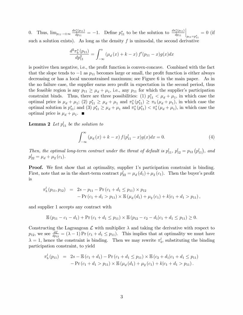
0. Thus, limp11!�1d�sb(p11)
dp11= �1. De�ne p�11 to be the solution to
d�sb(p11)
dp11
���p11=p�11
= 0 (if
such a solution exists). As long as the density f is unimodal, the second derivative
d2�sb (p11)
dp211=
Z �
�1(�d (x) + k � x) f 0(p11 � x)g(x)dx
is positive then negative, i.e., the pro�t function is convex-concave. Combined with the factthat the slope tends to �1 as p11 becomes large or small, the pro�t function is either alwaysdecreasing or has a local unconstrained maximum; see Figure 6 in the main paper. As inthe no failure case, the supplier earns zero pro�t in expectation in the second period, thusthe feasible region is any p11 � �d + �1, i.e., any p11 for which the supplier�s participationconstraint binds. Thus, there are three possibilities: (1) p�11 < �d + �1, in which case theoptimal price is �d + �1; (2) p
�11 � �d + �1 and �
sb (p
�11) � �b (�d + �1), in which case the
optimal solution is p�11; and (3) p�11 � �d + �1 and �sb (p�11) < �sb (�d + �1), in which case the
optimal price is �d + �1.
Lemma 2 Let pl11 be the solution toZ 1
�1(�d (x) + k � x) f(pl11 � x)g(x)dx = 0: (4)
Then, the optimal long-term contract under the threat of default is pl11, pl12 = p12
�pl11�, and
pl22 = �d + �2 (c1).
Proof. We �rst show that at optimality, supplier 1�s participation constraint is binding.First, note that as in the short-term contract pl22 = �d (d1)+�2 (c1). Then the buyer�s pro�tis
�lb (p11; p12) = 2s� p11 � Pr (c1 + d1 � p11)� p12�Pr (c1 + d1 > p11)� E (�d (d1) + �2 (c1) + kjc1 + d1 > p11) ;
and supplier 1 accepts any contract with
E (p11 � c1 � d1) + Pr (c1 + d1 � p11)� E (p12 � c2 � d1jc1 + d1 � p11) � 0:
Constructing the Lagrangean L with multiplier � and taking the derivative with respect top12, we see dL
dp12= (�� 1) Pr (c1 + d1 � p11). This implies that at optimality we must have
� = 1, hence the constraint is binding. Then we may rewrite �lb, substituting the bindingparticipation constraint, to yield
�lb (p11) = 2s� E (c1 + d1)� Pr (c1 + d1 � p11)� E (c2 + d1jc1 + d1 � p11)�Pr (c1 + d1 > p11)� E (�d (d1) + �2 (c1) + kjc1 + d1 > p11) :
3
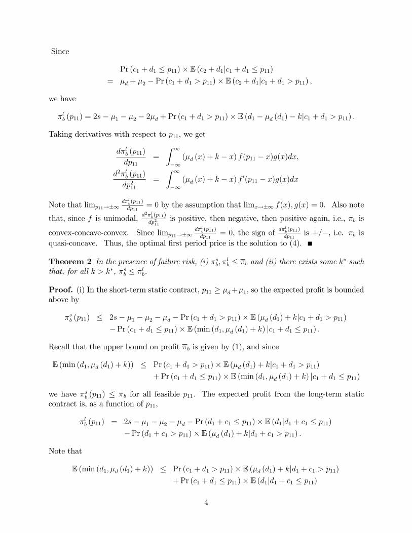
Since
Pr (c1 + d1 � p11)� E (c2 + d1jc1 + d1 � p11)= �d + �2 � Pr (c1 + d1 > p11)� E (c2 + d1jc1 + d1 > p11) ;
we have
�lb (p11) = 2s� �1 � �2 � 2�d + Pr (c1 + d1 > p11)� E (d1 � �d (d1)� kjc1 + d1 > p11) :
Taking derivatives with respect to p11, we get
d�lb (p11)
dp11=
Z 1
�1(�d (x) + k � x) f(p11 � x)g(x)dx;
d2�lb (p11)
dp211=
Z 1
�1(�d (x) + k � x) f 0(p11 � x)g(x)dx
Note that limp11!�1d�lb(p11)
dp11= 0 by the assumption that limx!�1 f(x); g(x) = 0. Also note
that, since f is unimodal, d2�lb(p11)
dp211is positive, then negative, then positive again, i.e., �b is
convex-concave-convex. Since limp11!�1d�lb(p11)
dp11= 0, the sign of d�
lb(p11)
dp11is +=�, i.e. �b is
quasi-concave. Thus, the optimal �rst period price is the solution to (4).
Theorem 2 In the presence of failure risk, (i) �sb; �lb � �b and (ii) there exists some k� such
that, for all k > k�, �sb � �lb.
Proof. (i) In the short-term static contract, p11 � �d+�1, so the expected pro�t is boundedabove by
�sb (p11) � 2s� �1 � �2 � �d � Pr (c1 + d1 > p11)� E (�d (d1) + kjc1 + d1 > p11)�Pr (c1 + d1 � p11)� E (min (d1; �d (d1) + k) jc1 + d1 � p11) :
Recall that the upper bound on pro�t �b is given by (1), and since
E (min (d1; �d (d1) + k)) � Pr (c1 + d1 > p11)� E (�d (d1) + kjc1 + d1 > p11)+Pr (c1 + d1 � p11)� E (min (d1; �d (d1) + k) jc1 + d1 � p11)
we have �sb (p11) � �b for all feasible p11. The expected pro�t from the long-term staticcontract is, as a function of p11,
�lb (p11) = 2s� �1 � �2 � �d � Pr (d1 + c1 � p11)� E (d1jd1 + c1 � p11)�Pr (d1 + c1 > p11)� E (�d (d1) + kjd1 + c1 > p11) :
Note that
E (min (d1; �d (d1) + k)) � Pr (c1 + d1 > p11)� E (�d (d1) + kjd1 + c1 > p11)+Pr (c1 + d1 � p11)� E (d1jd1 + c1 � p11)
4
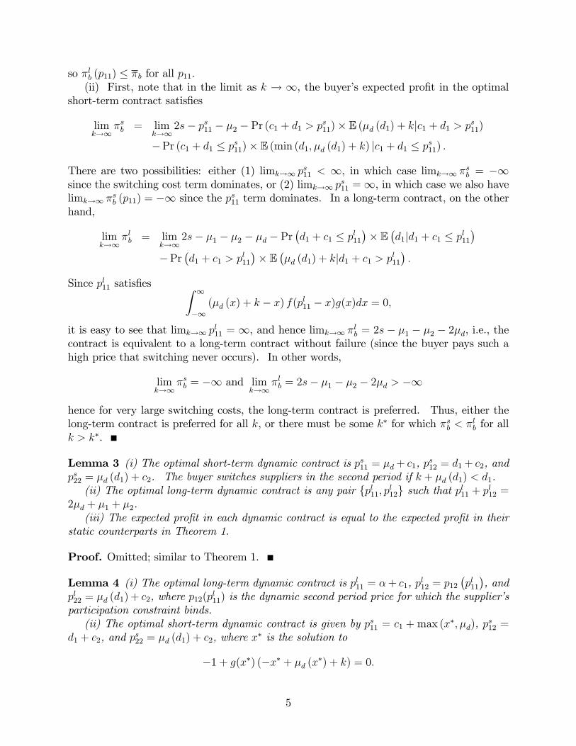
so �lb (p11) � �b for all p11.(ii) First, note that in the limit as k ! 1, the buyer�s expected pro�t in the optimal
short-term contract satis�es
limk!1
�sb = limk!1
2s� ps11 � �2 � Pr (c1 + d1 > ps11)� E (�d (d1) + kjc1 + d1 > ps11)
�Pr (c1 + d1 � ps11)� E (min (d1; �d (d1) + k) jc1 + d1 � ps11) :
There are two possibilities: either (1) limk!1 ps11 < 1, in which case limk!1 �
sb = �1
since the switching cost term dominates, or (2) limk!1 ps11 =1, in which case we also have
limk!1 �sb (p11) = �1 since the ps11 term dominates. In a long-term contract, on the other
hand,
limk!1
�lb = limk!1
2s� �1 � �2 � �d � Pr�d1 + c1 � pl11
�� E
�d1jd1 + c1 � pl11
��Pr
�d1 + c1 > p
l11
�� E
��d (d1) + kjd1 + c1 > pl11
�:
Since pl11 satis�es Z 1
�1(�d (x) + k � x) f(pl11 � x)g(x)dx = 0;
it is easy to see that limk!1 pl11 = 1, and hence limk!1 �
lb = 2s � �1 � �2 � 2�d, i.e., the
contract is equivalent to a long-term contract without failure (since the buyer pays such ahigh price that switching never occurs). In other words,
limk!1
�sb = �1 and limk!1
�lb = 2s� �1 � �2 � 2�d > �1
hence for very large switching costs, the long-term contract is preferred. Thus, either thelong-term contract is preferred for all k, or there must be some k� for which �sb < �
lb for all
k > k�.
Lemma 3 (i) The optimal short-term dynamic contract is ps11 = �d+ c1, ps12 = d1+ c2, and
ps22 = �d (d1) + c2. The buyer switches suppliers in the second period if k + �d (d1) < d1.(ii) The optimal long-term dynamic contract is any pair fpl11; pl12g such that pl11 + pl12 =
2�d + �1 + �2.(iii) The expected pro�t in each dynamic contract is equal to the expected pro�t in their
static counterparts in Theorem 1.
Proof. Omitted; similar to Theorem 1.
Lemma 4 (i) The optimal long-term dynamic contract is pl11 = �+ c1, pl12 = p12
�pl11�, and
pl22 = �d (d1) + c2, where p12(pl11) is the dynamic second period price for which the supplier�s
participation constraint binds.(ii) The optimal short-term dynamic contract is given by ps11 = c1 + max (x
�; �d), ps12 =
d1 + c2, and ps22 = �d (d1) + c2, where x� is the solution to
�1 + g(x�) (�x� + �d (x�) + k) = 0:
5
(iii) The long-term dynamic contract is preferred to the short-term dynamic contract, andyields expected pro�t equal to the system optimal expected pro�t without failure risk.
Proof. (i) With a dynamic long-term contract, the buyer o¤ers p11 = c1 + �1, p12 = c2 + �2,and p22 = c2 + �3, optimizing over �i, i = 1; 2; 3. Failure occurs if �1 < d1. For the samereasons as in the previous lemmas, pl22 = c2 + �d (d1). Thus, the buyer�s pro�t is
�b = 2s� �1 � �2 � �1 � Pr (�1 � d1)� p12 � Pr (�1 < d1)� (�d (d1) + k) ;
maximized subject to
�1 � �d + Pr (�1 � d1)� E (�2 � d1j�1 � d1) � 0: (5)
As in Lemma 4, one can show that the constraint is binding at any optimal solution byconstructing the Lagrangean. Thus, by substituting a binding constraint into the objectivefunction, we eliminate �2 and write the buyer�s pro�t as
�b = 2s� �1 � �2 � �d �Z �1
�1xg(x)dx�
Z 1
�1
(�d (x) + k) g(x)dx:
Optimizing over �1, we have
d�bd�1
= g(�1) (��1 + �d (�1) + k)
Since g(x) > 0 for all feasible x, �b is quasiconcave, and is maximized by �1 = �d (�1) + k,or �1 = �. Letting �2(�1) be the value of �2 such that (5) holds, we have pl11 = c1 + �,pl12 = c2 + �2(�1), and p
l22 = c2 + �d(d1). De�ning p12(p11) = c2 + �2(�1) yields the result.
(ii) In a dynamic short term contract, the buyer o¤ers p11 = c1 + �1, p12 = c2 + �2, andp22 = c2+ �3, optimizing over the various �. Failure occurs if �1 < d1. For the same reasonsas in the previous lemmas, �3 = �d (d1) and �2 = d1, and the buyer switches suppliers ifd1 > �d (d1) + k. This implies
�b = 2s� �1 � �2 � �1 � Pr (�1 � d1; �d (d1) + k � d1)� E (d1j�1 � d1; �d (d1) + k � d1)�Pr (�1 < d1)� E (�d (d1) + kj�1 < d1)�Pr (�d (d1) + k < d1)� E (�d (d1) + kj�d (d1) + k < d1) :
Supplier 1 accepts any contract with �1 � �d. Clearly there are two cases. In the �rst,�1 > �, so
�b = 2s� �1 � �2 � �1 � Pr (� � d1)� E (d1j�d + k � d1)�Pr (� < d1)� E (�d (d1) + kj� < d1) :
The derivative is thus d�bd�1
= �1 and the optimal solution is �1 = �. In the second case,
6

�1 � �, so
�b = 2s� �1 � �2 � �1 �Z �1
�1xg(x)dx�
Z 1
�1
(�d (x) + k) g(x)dx
and d�bd�1
= �1 + g(�1) (��1 + �d (�1) + k). Since g(x) > 0 for all x, the second term inthis expression is negative for �1 � �, then positive for �1 < �, thus d�b
d�1is either always
negative (resulting in the optimal solution being boundary, �1 = �d) or has a unique zero inthe interval �d � �1 < �.(iii) The pro�t from the short-term contract is
�b = 2s� �1 � �2 � �1 �Z �1
�1xg(x)dx�
Z 1
�1
(�d (x) + k) g(x)dx
� 2s� �1 � �2 � �d �Z �1
�1xg(x)dx�
Z 1
�1
(�d (x) + k) g(x)dx;
since �d � �1 < �. Comparing this to the long-term contract�s pro�t of �b, we see that thedi¤erence between these two is
�b � �b � Pr (�1 � d1 < �)� E (�d (d1) + k � d1j (�1 � d1 < �)) > 0
hence the long-term dynamic contract is always preferred.
2. Contingent Transfer Payments and Loans
In what follows, we allow the buyer the option of making a transfer payment T to the supplierin the second period. The purpose of this transfer payment is to help support the supplierin the event that bankruptcy occurs at the end of the �rst period; that is, following a loss inthe �rst period, if the buyer raises the total capital level of the supplier to zero or higher thesupplier is spared from bankruptcy and may continue to do business with the buyer in thesecond period. See Babich (2006) for an analysis of why such threshold transfer paymentsmay be optimal when suppliers face default risk.We assume that some proportion r � 0 of the transfer payment T is repaid to the buyer
at the end of the second period. If r = 0, then no amount is paid to the buyer; in thiscase, T is a direct operating subsidy. If r > 0, then T is a loan, some fraction of which isrepaid to the buyer. If r > 1, then the buyer charges interest on the loan. For simplicity,we assume that r is exogenously determined (i.e., the �rms do not bargain over the interestrate or repayment percentage of any transfer payment or loan). We also assume that thesupplier only repays what he can based on pro�ts in the second period.It is easy to see that if the supplier does not enter bankruptcy, it is optimal to o¤er no
transfer payment, T = 0. If the supplier does enter bankruptcy, then let T (y) = �p11 +c1 + d1 + y, where y � 0 is the excess cash that the buyer provides in the transfer paymentthat raises the supplier�s capital level above zero. Let R = min
�rT; �+12
�be the repayment
amount, where �+12 = (p12 � c2 � d1 + y)+ is the positive part of the incumbent supplier�stotal pro�t at the end of the second period. Conditional on a transfer payment T (y) having
7
been made to a bankrupt supplier, the buyer�s optimization problem in contracting with theincumbent supplier in the second period is
maxy;p12
s� p12 + ER
s.t. p12 � d1 � E (c2 +R) + y � 0:
Di¤erentiating the objective with respect to p12, we see
d (s� p12 + ER)dp12
= �1 + Pr (rT > p12 � c2 � d1 + y > 0) < 0;
i.e., pro�t is a decreasing function of price, so the participation constraint will be binding.By inserting the binding participation constraint into the objective function, we see that thebuyer�s expected pro�t from contracting with the incumbent supplier in the second periodis, after subtracting the cost of the transfer payment,
s� d1 � E (c2) + y � T:
The y term in this expression sums to zero with the y term in T , thus, in general, the optimaltransfer payment satis�es y = 0, implying
T = (�p11 + c1 + d1)+ ;
while the cost of contracting with a bankrupt supplier and providing an operating subsidyis d1+ �2(c1) + T . Note that this expression is independent of r, i.e., it does not depend onwhether or not the loan is repaid to the buyer. The reason for this is that the buyer extractsall of the supplier�s surplus whether or not the loan is repaid, making the participationconstraint binding; hence, if the supplier is to repay the buyer at the end of the secondperiod, the buyer must compensate the supplier by paying a higher contract price. Since thebuyer is already extracting all surplus from the supplier, he cannot extract further surplus,and his expected pro�t from contracting with the bankrupt supplier is thus independent ofthe magnitude of repayment. Thus, for the remainder of the analysis, we may ignore theprecise value of r, and assume that the buyer pays a price of p12 = d1+�2(c1)+T to subsidizeand do business with a bankrupt supplier in period 2.It may not be in the best interests of the buyer to support the bankrupt supplier. In
particular, if the total expected procurement cost plus the necessary transfer payment exceedthe total cost of switching to a new supplier, the buyer will choose the alternative supplier.In other words, if
d1 + T � �d(d1) + k; (6)
then it is optimal for the buyer to switch suppliers. We now de�ne the following function:
! (p11; c1) � fx : 2x� �d(x) = p11 � c1 + kg ;
which represents the value of the idiosyncratic cost d1 such that (6) holds with equality forgiven values of p11, c1, and k. Since, by assumption, 2x� �d(x) is monotonically increasingin x, there is a unique value of ! (p11; c1) for each p11 and c1. Implicitly di¤erentiating
8
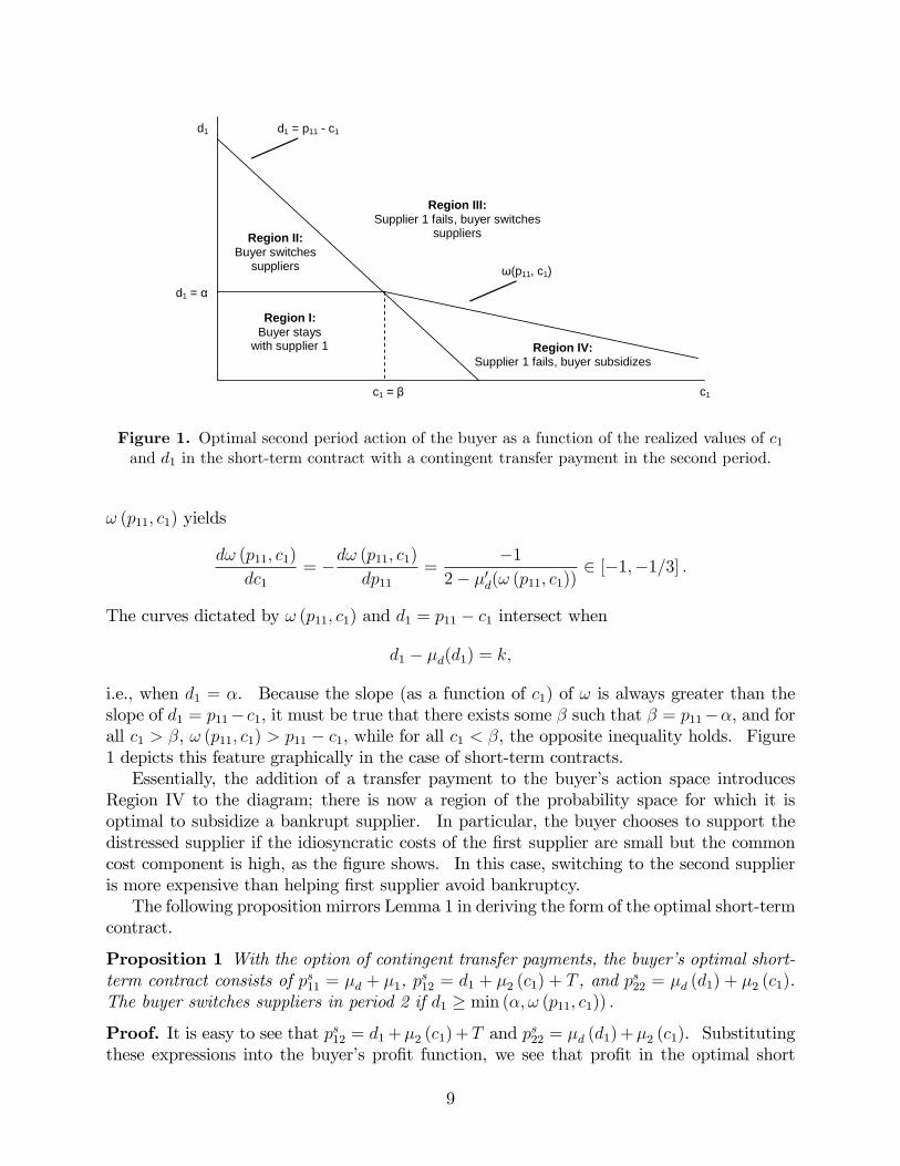
Region III:Supplier 1 fails, buyer switches
suppliers
c1
d1 d1 = p11 c1
Region I:Buyer stays
with supplier 1
Region II:Buyer switches
suppliers
d1 = α
Region IV:Supplier 1 fails, buyer subsidizes
ω(p11, c1)
c1 = β
Figure 1. Optimal second period action of the buyer as a function of the realized values of c1and d1 in the short-term contract with a contingent transfer payment in the second period.
! (p11; c1) yields
d! (p11; c1)
dc1= �d! (p11; c1)
dp11=
�12� �0d(! (p11; c1))
2 [�1;�1=3] :
The curves dictated by ! (p11; c1) and d1 = p11 � c1 intersect when
d1 � �d(d1) = k;
i.e., when d1 = �. Because the slope (as a function of c1) of ! is always greater than theslope of d1 = p11� c1, it must be true that there exists some � such that � = p11��, and forall c1 > �, ! (p11; c1) > p11 � c1, while for all c1 < �, the opposite inequality holds. Figure1 depicts this feature graphically in the case of short-term contracts.Essentially, the addition of a transfer payment to the buyer�s action space introduces
Region IV to the diagram; there is now a region of the probability space for which it isoptimal to subsidize a bankrupt supplier. In particular, the buyer chooses to support thedistressed supplier if the idiosyncratic costs of the �rst supplier are small but the commoncost component is high, as the �gure shows. In this case, switching to the second supplieris more expensive than helping �rst supplier avoid bankruptcy.The following proposition mirrors Lemma 1 in deriving the form of the optimal short-term
contract.
Proposition 1 With the option of contingent transfer payments, the buyer�s optimal short-term contract consists of ps11 = �d + �1, p
s12 = d1 + �2 (c1) + T , and p
s22 = �d (d1) + �2 (c1).
The buyer switches suppliers in period 2 if d1 � min (�; ! (p11; c1)) :
Proof. It is easy to see that ps12 = d1+�2 (c1)+T and ps22 = �d (d1)+�2 (c1). Substituting
these expressions into the buyer�s pro�t function, we see that pro�t in the optimal short
9
term contract as a function of p11 is
�sb (p11) = 2s� �2 � p11 � Emin (d1 + T; �d (d1) + k) ;
where T = (c1 � d1 � p11)+. Di¤erentiating this expression with respect to p11, we have
d�sb (p11)
dp11= �1 + Pr (Region IV) � 0;
where Pr (Region IV) denotes the probability of Region IV in Figure 1, i.e. the probabilitythat c1 > � and ! (p11; c1) > d1 > p11 � c1. Since pro�t is decreasing in p11, it is optimal toset p11 as small as possible such that the supplier�s participation constraint is satis�ed, i.e.,ps11 = �d + �1.The following proposition describes the optimal two-period contract with contingent
transfer payments. In the analysis below, we assume that long-term contracts are renegoti-ated if bankruptcy occurs and the buyer subsidizes the bankrupt supplier. This is re�ectiveof the fact that often, when working with bankrupt suppliers, buyers must pay court-orderedprice increases rather than continue with the terms of existing (likely unpro�table) contracts(see, for example, the case of Collins & Aikman discussed in Barkholz and Sherefkin 2007).We note that our results continue to hold even if prices are not renegotiated (see §3 of thisappendix, which can be shown to apply to the case of contingent transfer payments as well)although the �rst order condition changes slightly (in particular, the expression for ! (p11; t)changes).
Proposition 2 Let pl11 be the solution toZ 1
p11��f (t) g (! (p11; t))
@! (p11; t)
@p11(! (p11; t) + t� p11) dt (7)
+
Z 1
�
(k + �d (x)� x) f (p11 � x) g (x) dx = 0:
Then, the optimal long-term contract under the threat of default is pl11, pl12 = p12
�pl11�, and
pl22 = �d + �2 (c1).
Proof. We �rst show that at optimality, supplier 1�s participation constraint is binding.Note that as in the short-term contract, pl22 = �d (d1) + �2 (c1), and furthermore due tothe renegotiation of the long-term contract if failure occurs, the cost of contracting with abankrupt supplier is d1+�2 (c1)+T (e¤ectively, regardless of the amount of loan repayment).Then the buyer�s pro�t is
�lb (p11; p12) = 2s� p11 � Pr (Region I,II)E (p12jRegion I,II)�Pr (Region IV)E (d1 + �2 (c1) + T jRegion IV)�Pr (Region III)E (�d (d1) + �2 (c1) + kjRegion III) ;
10
where T = (�p11 + c1 + d1)+, and supplier 1 accepts any contract with
E (p11 � c1 � d1) + Pr (Region I,II)E (p12 � c2 � d1jRegion I,II)+ Pr (Region IV)E (T jRegion IV) � 0:
Note that since the participation constraint of the supplier now considers two periods, thetransfer payment T (and potential repayment R) are taken into account. Constructing theLagrangean L with multiplier � and taking the derivative with respect to p12, we see
dLdp12
= (�� 1) Pr (Region I,II) :
This implies that at optimality we must have � = 1, hence the constraint is binding. Thenwe may rewrite �b, substituting the binding participation constraint, which yields
�lb (p11) = 2s� �1 � �2 � �d � Pr (Regions I,II,IV)E (d1jRegions I,II,IV)�Pr (Region III)E (�d (d1) + kjRegion III) :
Di¤erentiating with respect to p11, we have
d�lb (p11)
dp11=
Z 1
p11��f (t) g (! (p11; t))
@! (p11; t)
@p11(! (p11; t) + t� p11) dt
+
Z 1
�
(k + �d (x)� x) f (p11 � x) g (x) dx
The �rst term is positive (since @!(p11;t)@p11
is positive) while the second term is negative. Fur-
thermore, note that limp11!�1d�lb(p11)
dp11= 0 by the assumption that limx!�1 f(x); g(x) = 0,
together with the fact that
limp11!�1
! (p11; c1) = limp11!�1
fx : 2x� �d(x) = p11 � c1 + kg = �1:
Di¤erentiating once more, we have
d2�lb (p11)
dp211=
Z 1
p11��f (t) g (! (p11; t))
@! (p11; t)
@p11
�@! (p11; t)
@p11� 1�dt
+
Z 1
p11��f (t) g (! (p11; t))
@2! (p11; t)
@p211(t� p11 + ! (p11; t)) dt
+
Z 1
p11��f (t) g0 (! (p11; t))
@! (p11; t)
@p11
2
(t� p11 + ! (p11; t)) dt
+
Z 1
�
(�d (x) + k � x) f 0 (p11 � x) g (x) dx:
11
Note that in the limit as p11 !1, the �rst three integrals converge to zero, and hence
limp11!1
d2�lb (p11)
dp211= lim
p11!1
Z 1
�
(�d (x) + k � x) f 0 (p11 � x) g (x) dx � 0
Thus, as p11 becomes large,d�lb(p11)
dp11tends to be increasing towards zero, i.e., it is negative,
and hence the optimal �rst period price solves the �rst order condition, d�lb(p11)
dp11= 0.
Finally, Proposition 3 demonstrates that the primary result of the paper holds: namely,long-term contracts are preferred if switching costs are high, and neither contract type co-ordinates the system in general. This proposition is referenced in Theorem 3 of the paper.
Proposition 3 In the presence of failure risk with contingent transfer payments or loans,(i) �sb; �
lb � �b and (ii) there exists some k� such that, for all k > k�, �sb � �lb.
Proof. (i) In the case of the short-term contract, by substituting the binding participationconstraint of supplier 1 into the buyer�s pro�t function, we see that the buyer�s pro�t underthe optimal single period contract is
�sb (p11) = 2s� �1 � �2 � �d � Emin (d1 + T; �d (d1) + k) ;
Since T � 0, it is easy to see that
�sb � 2s� �1 � �2 � �d � E (min (d1; �d (d1) + k)) = �b:
The expected pro�t from the long-term static contract is
�lb = 2s� �1 � �2 � �d � Pr (Regions I,II,IV)E (d1jRegions I,II,IV)�Pr (Region III)E (�d (d1) + kjRegion III) :
Again, it follows by de�nition that
�lb � 2s� �1 � �2 � �d � E (min (d1; �d (d1) + k)) = �b:
(ii) In the case of the short-term contract, as k !1, we have
limk!1
�sb = limk!1
2s� �1 � �2 � �d � Emin (d1 + T; �d (d1) + k)
= limk!1
2s� �1 � �2 � 2�d � E�(d1 + c1 � �1 � �d)
+� :In the long-term contract, on the other hand, from (7) we see that limk!1 p
l11 =1, implying
limk!1 Pr (Regions III,IV) = 0, and hence
limk!1
�lb = 2s� �1 � �2 � 2�d:
Thus, for large k, the long-term contract is preferred to the short-term contract, and theproposition holds.
12
As discussed in the main text of the paper, the assumption that any transfer payment ismade at the start of the second period is key. However, if this assumption is relaxed, theresults of the above theorem continue hold if one of several alternative conditions are met.We refer the reader to §7.2 of the main text for a discussion of this point.
3. Renegotiation
If the buyer is capable of renegotiating the long-term contract, then he will do so wheneverthe renegotiated price is lower than the contract price. Assume that during the rene-gotiation process, the supplier will accept any contract with non-negative pro�t in period2. In that case, the renegotiated price is d1 + �2 (c1). The buyer then pays the suppliermin (p12; d1 + �2 (c1)) in the second period, where p12 is the second period contract price.The pro�t to the buyer is thus
�b = 2s� p11 � Pr (p11 � c1 + d1)� E (min (p12; d1 + �2 (c1)) jp11 � c1 + d1)�Pr (p11 < c1 + d1)� E (�d (d1) + �2 (c1) + kjp11 < c1 + d1) :
There are subsequently two cases: either the supplier recognizes that the buyer will rene-gotiate the contract (and hence takes this into account in the participation constraint), orthe supplier does not recognize that renegotiation will occur. In the former case, supplier 1accepts any contract with
E (p11 � c1 � d1) + Pr (p11 � c1 + d1)E (min (p12; d1 + �2 (c1))� c2 � d1jp11 � c1 + d1) � 0:
As in the proof of Lemma 2, we may construct the Lagrangean L with multiplier � and takethe derivative with respect to p12 to see that dL
dp12= (�� 1) Pr (p11 � c1 + d1; p12 � d1 + �2 (c1)).
This implies that at optimality it must be true that � = 1, and the constraint is binding.We may then rewrite �b, substituting the binding participation constraint, to yield
�lb (p11) = 2s� �1 � �2 � 2�d +Z 1
�1
Z 1
p11�x(x� �d (x)� k) f(t)g(x)dtdx;
which is precisely the same expression as the model without buyer renegotiation.On the other hand, if the supplier does not recognize that renegotiation will occur, then
the buyer�s pro�t is clearly higher than in the no-renegotiation case. Thus, the pro�tabilityof the long-term contracts is increased relative to the value of short-term contracts, and theresults of the model continue to hold.
4. Normally Distributed Costs
Theorem 4. (i) The optimal expected pro�t under all contract types is decreasing in �d.(ii) The di¤erence between the system optimal (long-term dynamic) pro�t and the pro�t
under the long-term static contract is decreasing in �d. In the limit as �d ! 1, pro�ts areequal.(iii) The centralized system optimal expected pro�t is increasing in �d.
13
Proof. (i) Recall that, from the properties of the bivariate normal distribution, theexpected value of d2 conditional on d1 = x is
�d (x) = (1� �d)�d + �dx. (8)
Using (8) and di¤erentiating �b, we see that for the long-term dynamic contract,
d�bd�d
= ��d + Emin (d1; �d + k= (1� �d))�k
1� �dG (�d + k= (1� �d)) < 0:
Now turning to the long-term static contract, by di¤erentiating �lb(p11) and using the Enve-lope Theorem,
d�lbd�d
=@�lb@�d
=
Z 1
�1
Z 1
pl11�x(�x+ �d) f(t)g(x)dtdx
= E��d1 + �djd1 > pl11 � c1
�Pr�d1 > p
l11 � c1
�< 0:
Finally, consider the short-term static contract. Applying the Envelope Theorem to �sb (p11),
d�sbd�d
=@�sb@�d
=
Z 1
�
(�d � x) g(x)dtdx+Z �
�1
Z 1
ps11�x(�d � x) f(t)g(x)dtdx � 0:
(ii) Consider the e¤ect of taking the limit as �d ! 1. Then, �b = 2s � 2�c � 2�d, andsince lim�d!1 p
�11 = 1, �lb(p11) = 2s � 2�c � 2�d as well, thus the contracts are equivalent.
To prove the �rst part of the proposition, by examining d�bd�d
and d�lbd�d
and noting that in the
long-term static contract p�11 = �c + �d + k= (1� �d), it can be shown that d2�bd�2d
> 0 andd2�lbd�2d
> 0. Since �b > �lb for �d < 1, both functions are convex and decreasing, and they
converge when �d = 1, it must be true thatd(�b��lb)
d�d< 0, i.e., the functions are smoothly
converging to one another.(iii) Using (8) and di¤erentiating �b, we see that for the long-term dynamic contract,
d�bd�d
= � d
d�d(Emin (d1; �d + k= (1� �d))) :
This expression is merely the negative of a newsvendor expected sales function. It is wellknown that expected sales decrease as a function of standard deviation in a newsvendor withnormally distributed demand, hence d
d�d(Emin (d1; �d + k= (1� �d))) < 0 and thus d�b
d�d> 0.
5. Numerical Study
To study the magnitude of k� (the switching cost above which long-term contracts are pre-ferred), we calculated this critical switching cost both with and without transfer paymentsfor every combination of the following parameters: �d = f1; 2; 3g, �1 = �2 = f1; 2; 3g,�d = f1; 3; 6g, �1 = �2 = f1; 3; 6g, and �d = f�0:5; 0; 0:5g, where costs are normally dis-
14
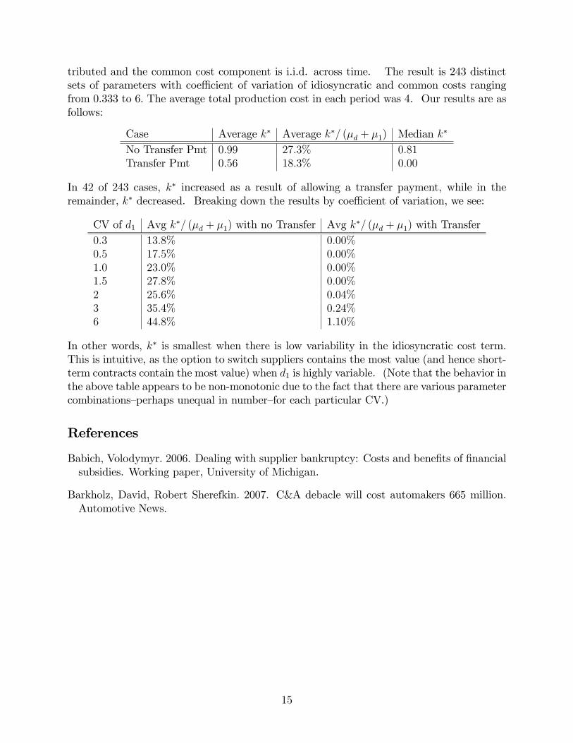
tributed and the common cost component is i.i.d. across time. The result is 243 distinctsets of parameters with coe¢ cient of variation of idiosyncratic and common costs rangingfrom 0.333 to 6. The average total production cost in each period was 4. Our results are asfollows:
Case Average k� Average k�= (�d + �1) Median k�
No Transfer Pmt 0:99 27:3% 0:81Transfer Pmt 0:56 18:3% 0:00
In 42 of 243 cases, k� increased as a result of allowing a transfer payment, while in theremainder, k� decreased. Breaking down the results by coe¢ cient of variation, we see:
CV of d1 Avg k�= (�d + �1) with no Transfer Avg k�= (�d + �1) with Transfer0:3 13:8% 0:00%0:5 17:5% 0:00%1:0 23:0% 0:00%1:5 27:8% 0:00%2 25:6% 0:04%3 35:4% 0:24%6 44:8% 1:10%
In other words, k� is smallest when there is low variability in the idiosyncratic cost term.This is intuitive, as the option to switch suppliers contains the most value (and hence short-term contracts contain the most value) when d1 is highly variable. (Note that the behavior inthe above table appears to be non-monotonic due to the fact that there are various parametercombinations�perhaps unequal in number�for each particular CV.)
References
Babich, Volodymyr. 2006. Dealing with supplier bankruptcy: Costs and bene�ts of �nancialsubsidies. Working paper, University of Michigan.
Barkholz, David, Robert Sherefkin. 2007. C&A debacle will cost automakers 665 million.Automotive News.
15