long-term ecological monitoring protocol for small …

Small mammal populations have been monitored as part of the Denali LTEM program

from its beginning in 1992. One aspect of this agreement is to maintain the small mammal

monitoring effort in Rock Creek and other drainages near park headquarters (this aspect

of the work is actually paid for by the NPS, via the USGS, to simplify contracting

arrangements). The research aspect of this agreement addresses the question of how to

sample small mammal populations at larger geographic scales.

The Denali LTEM program has always billed itself as an "integrated" watershed approach. The

intent to "integrate" was implied by the arrangement of study effort in the Rock Creek watershed

(i.e, the collocation of data collection efforts). However, mechanisms to promote integration of

results have not yet been developed, and all reporting thus far has focused on individual study

efforts. By 1997, it was clear that integration was not going to occur unless some specific effort

was put into it. Thus, one purpose of this agreement is to throw some resources at the

"integration" question.

Taken over

---------------- Draft 1.2 --------------

Denali Long-term Ecological Monitoring Program

Protocol For Long-term Monitoring Of Small Mammal Populations

2005

Eric Rexstad, Ed Debevec, and Cam MacDonald

Institute of Arctic Biology

University of Alaska Fairbanks

Fairbanks AK

---------------- DRAFT 1.2 --------------

TABLE OF CONTENTS

SOP 1 — SOME NECESSARY BACKGROUND .................................................................... 1

1.1 Brief Project History ............................................................................................................. 1

1.2 Calculating Density Using Capture-Recapture ..................................................................... 1

SOP 2 — BEFORE TRAPPING STARTS ................................................................................. 2

2.1 Field Season Preparations ..................................................................................................... 2

2.2 Field Season Sampling Schedule .......................................................................................... 3

2.3 Initial Grid Setup: ................................................................................................................. 4

SOP 3 — TRAPPING SESSION OVERVIEW ......................................................................... 5

3.1 Getting to the Site (Day 1) .................................................................................................... 5

3.2 Setting Traps (Day 1) ............................................................................................................ 5

3.3 Checking Traps (Day 2 to 5) ................................................................................................. 6

3.4 End of the Sampling Week (Day 6) ...................................................................................... 7

3.5 ―Weekends‖ (Day 7) ............................................................................................................. 7

SOP 4 — PROCESSING SMALL MAMMALS ....................................................................... 8

4.1 Species Identification ............................................................................................................ 8

4.2 Passive Integrated Transponders (PIT tags) ......................................................................... 8

4.3 Handling Techniques ............................................................................................................ 9

4.6 Trap Maintenance ............................................................................................................... 13

4.7 Trapping Mortalities ........................................................................................................... 13

SOP 5 — DATA MANAGEMENT AND ANALYSIS ............................................................ 14

5.1 Data entry ............................................................................................................................ 14

5.2 Downloading palmtop to laptop ......................................................................................... 14

5.3 Summarizing data and creating capture histories ............................................................... 15

5.5 Calculating abundance estimates using CAPTURE ........................................................... 16

5.6 Data archival in MS Access ................................................................................................ 19

5.7 WEB presentation of data ................................................................................................... 20

SOP 6 — WORKING IN THE BACKCOUNTRY ................................................................. 20

6.1 Low-impact Camping ......................................................................................................... 20

6.2 Bear Etiquette: .................................................................................................................... 21

6.3 Necessary Clothing: ............................................................................................................ 23

6.4 Camping Equipment ........................................................................................................... 23

SOP 7 — END OF SEASON ...................................................................................................... 25

7.1 Cleanup ............................................................................................................................... 25

7.2 Future Suggestions: ............................................................................................................. 25

APPENDIX 1: SITE DESCRIPTIONS .................................................................................... 27

APPENDIX 2: S-PLUS FUNCTIONS ...................................................................................... 32

APPENDIX 3: SMALL MAMMAL DATABASE ................................................................... 39

1

SOP 1 — SOME NECESSARY BACKGROUND

1.1 Brief Project History

As part of the Denali Long-term Ecological Monitoring program (LTEM), small mammals have

been monitored in the Rock Creek drainage since 1992. The first expansion of this monitoring

program took place in 1995 with additional sampling near Wonder Lake at the western end of the

park road (approximately 100 km from Rock Creek). A second expansion occurred in 1997 when

three additional watersheds in the Rock Creek area were also sampled. Most recently, and with

the hope of increasing our understanding of small mammal spatial dynamics throughout Denali,

sampling was again expanded in 2000 to include three new sites in addition to those previously

sampled at Rock Creek and Wonder Lake. The new sites are spaced between Rock Creek and

Wonder Lake at approximately 25 km intervals (if a crow) and are located within 5 km of the

park road. Also in 2000, the small mammal monitoring program went online. The WEB is an

ideal medium to concisely and accessibly present a great deal of information: maps, coordinates,

pictures, data, reports, etc. Check it out!

Web site: (http://mercury.bio.uaf.edu/~edebevec.staff/denali-sites/index.html)

1.2 Calculating Abundance Using Capture-Recapture

The goal of the small mammal research program is to determine the abundance of study species

at each grid within each trapping session. Abundances can then be compared between capture

sessions, study sites, and years. This study uses capture-recapture methods and models to

estimate abundance. All capture-recapture models follow the same reasoning: if animals are

marked and released, the proportion of marked individuals in subsequent capture sessions should

be representative of the proportion marked in the entire population. Analyses of data from

previous years suggested that 12 capture sessions (3 per day for 4 days) were sufficient to

generate precise population estimates.

2

SOP 2 — BEFORE TRAPPING STARTS

2.1 Field Season Preparations

Ideally, the field crew will arrive in Fairbanks ten days prior to the start of the first trapping

session (see Box 2.1). The first three days will be spent in Fairbanks organizing field equipment,

acquiring provisions, and examining museum specimens to aid field identifications. The next

week will be spent in Denali setting up the trapping grids, hauling traps to the study sites, and

networking with the NPS resource staff and bear technicians. Formal training will all be ‗hands-

on‘ and will occur during the first week of sampling when the principal investigator (Dr. Eric

Rexstad) will be in the field with the crew.

Depending on the vehicle being used, two or three road trips will be required to get all the

necessary gear from Fairbanks to Denali. The bulk of the cargo will be traps (~1200) and food

for the first half of the season. Check with the LTEM coordinator as to where to store equipment

at Denali.

Box 2.1: The First Ten Days

To be done in Fairbanks …

Complete necessary paperwork to start employment process (see Marta Rm #309)

View museum specimens (target and non-target species)

Purchase food from Fred Meyers (for purchase order see Genelle Rm #308)

Purchase bait from Alaska Feed (2 x 50 lb bag of cracked sunflower seeds)

Microwave bait to prevent germination (100 lb x 1.5 minutes on high per pound)

Purchase additional equipment as required (see accompanying checklists)

Ensure field equipment is functional (particularly palmtops, laptops, and tents)

Review data handling and downloading procedures with Eric

Upon arrival in Denali …

Meet with LTEM coordinator

Pickup road permit (arranged by LTEM coordinator)

Pickup radio from dispatch (discuss radio protocol with dispatch)

Watch ―Rules of the Road‖ video, an instructional and inspirational video on driving the park road

Watch ―Denali Backcountry Video‖ at the Visitors Center

Meet with Bear Technicians

Get bear barrels (4 large) from Bear Techs or backcountry desk

Arrange for equipment storage and refrigeration (for mortalities) with LTEM coordinator

Checkout living arrangements for weekend accommodations

Setting up …

Five days will be needed to setup grids at all study sites (see section 2.3)

All 400 traps can be brought to the Rock Creek site as it is the first site trapped

150 traps can also be cached at each site at this time

3

2.2 Field Season Sampling Schedule

Like most biological field seasons, particularly those that must make the most of the short sub-

arctic summer, the workload can be described as intense. Have no illusions, this is not a standard

40-hour/week job.

Over the course of the summer, the study sites are each sampled twice except for Rock Creek

which is sampled three times. A sampling session involves 12 trap checks, 3 per day for 4 days

(Monday thru Thursday). Sundays are for driving to the site, hauling required gear (2 or 3 trips),

pitching camp, and setting the traps. Fridays are for packing down camp, hauling gear out of the

site (2 or 3 trips), and driving back to Healy. Saturdays are for data processing and food pack-up

for the next sampling session (see Box 2.2).

Box 2.2: Sampling Schedules

2000 Seasonal Sampling Schedule:

June 12 Start work

June 18-23 Rock Creek

June 25-30 Teklanika

July 2-7 Wonder Lake

July 9-14 Stony Creek

July 16-21 Polychrome

July 23-28 Rock Creek

July 30-4 Teklanika

August 6-11 Wonder Lake

August 13-18 Stony Creek*

August 20-25 Polychrome

August 27-1 Rock Creek

September 1-4 Cleanup

*snowed out

2000 Weekly Sampling Schedule:

Sun Mon Tue Wed Thu Fri Sat

Pack ALL gear Trap check 0600 600 600 600 Pack-up camp Process data

Drive to site 1300 1300 1300 1300 Haul-out gear (x 2) Pack food

Haul gear (2-3 trips) 2000 2000 2000 2000 Drive to Healy Dry gear

Setup camp Laundry

Set traps

4

2.3 Initial Grid Setup:

There are four trapping grids at Rock Creek and three trapping grids at all other locations. Each

grid covers an area 90 m x 90 m (0.81 hectares) and consists of 100 Sherman live-traps spaced at

10 m intervals. Individual trap locations are marked with flagging tape during the field season.

However, to minimize visual impacts, all flagging tape has to be removed at the end of each field

season. All trapping grids, therefore, need to be re-established during the first week of each field

season (see Box 2.3). To make the most of this first week, 150 traps can also be hauled out to

each site (400 to Rock Creek) and then cached until needed.

Box 2.3: Establishing a trapping grid*

1. Use the GPS unit to navigate to one corner of a grid (see Appendix 1 for coordinates)

2. Mark this corner with flagging tape

3. Have a second person use the GPS to navigate to the second corner

4. Distance between these corners should be 90m; adjust using the laser rangefinder#

5. Have second person walk towards first flag while the other person ‗shoots= the approaching person

with the rangefinder

6. Tie flagging to vegetation at 10 m intervals

Now that the baseline is established, the remaining trap locations need to be determined:

7. Have one person use a compass to walk a perpendicular bearing away from each baseline flag in the

direction shown on the site maps (Appendix 1)

8. Again the rangefinder is used to determine 10 m intervals; flags are placed at each of these intervals

9. Flag adjacent lines with different colors to help prevent wandering onto the wrong line when checking

traps (e.g. 7A-7J orange, 6A-6J blue, 5A-5J orange)

10. Use a sharpie marker to write the correct X and Y coordinates of each trap location (e.g. 5G, 9A) on

each flag as shown on the site maps

Summary of equipment needed to setup a trapping grid

GPS unit

laser rangefinder

compass with sighting mirror

flagging tape (two colors)

sharpie marker

* it should take 2-3 hours to accurately establish each trapping grid # a simple monocular that displays distance in viewer when button is pushed

flagging should be visible enough to facilitate trap checking without attracting unnecessary attention

there is ongoing discussion with NPS as to the most appropriate colors for flagging the small mammal grids

5

SOP 3 — TRAPPING SESSION OVERVIEW

3.1 Getting to the Site (Day 1)

Each trapping session begins with the setting of traps on Sunday evening. Depending on what

site you are doing and how many traps need to be hauled to the site, the day will start sometime

between 0700 and 1500 (see Box 3.1). For instance, if you are going to the Stony Creek site and

you have 160 traps to bring in, the day should begin around 9am: 3 hour drive, 1.5 hour for first

haul with personal gear and food, 1 hours to setup camp and eat lunch, 1 hour back out to

vehicle, 1.5 hour for second haul out with traps and remaining gear, 1 hour for dinner break, 3-4

hours to setup trapping grids. Traps can be setup anytime after 1830.

3.2 Setting Traps (Day 1)

The folding traps used in the small mammal program are manufactured by the H. B. Sherman

Company (7.6cm x 8.9cm x 22.9cm). The traps are sufficient to catch the largest individuals

studied yet sensitive enough to capture shrews.

Each trap is baited with approximately one tablespoon of cracked sunflower seeds. The seeds

have to be microwaved beforehand to further prevent germination (1.5 minutes on high per

pound). To minimize thermal stress of the animals, bedding material is also put in each trap in

the form of a nestlet, a 6cm x 6cm x 1cm square of compressed cotton. Nestlets are more

compact than the commonly used batten and thus easier to carry into the backcountry. Nestlets

can be acquired from animal supply stores.

Box 3.1: Latest Sunday departure times from headquarters*

Rock Creek 1500

Teklanika 1200

Polychrome 1000

Stony Creek 0900

Wonder Lake 1000

* assuming a two-person crew and 160 traps to be carried out

6

Eric Rexstad (PI) will demonstrate the proper technique for setting traps in the field during the

first trapping session. Basically, traps are unfolded until they lock into an upright position. The

front door is then pushed all the way open until the trigger catches and locks the door in the open

position. The door will close when an animal enters the trap and steps on the treadle in the back

of the trap. Depression of the treadle causes the trigger to release the door which then springs

closed. Trap tension (how easily a trap will spring) is adjusted by manually manipulating the

trigger. Traps should spring when lightly tapped. Additionally, make sure debris (brush, dried

feces, soiled nestlets, or bait) doesn‘t get stuck under the treadle and prevent it from being

depressed.

Traps are placed so as to be visible from the trap station flag, usually within 1m. It is important

that traps are level and that the opening is not obstructed. Depending on vegetation cover, traps

can be partially nestled into vegetation or left exposed.

3.3 Checking Traps (Day 2 to 5)

Monday through Thursday (inclusive) traps are checked three times a day. Three trap checks are

the most that can be asked of the field crew while minimizing the time animals spend confined in

traps.

The first daily trap check begins at 0600 on Monday morning. This necessitates alarm clocks

being set for 0530-0545. It is wise to have both members of the field crew set an alarm clock(s).

Depending on the need for a morning energy boost, some crewmembers will desire food (power

bar etc.) prior to starting the first check. The morning check is usually the busiest with respect to

the number of captures as small mammals tend to be more active overnight and the interval since

last trap checks is greatest at this time. Expect to spend up to 4 hours on the morning check

depending on the number of captures; if it is an exceptionally busy year it could be longer still

(good luck!). At the completion of each check, it is important to organize for the next check:

process mortalities, re-supply bait and nestlets, and save the data.

The second daily trap check begins at 1300 hours. Because this is usually the lightest check,

additional effort is spent checking the working performance of each trap (see trap maintenance)

and re-baiting if necessary. This check should hopefully be done by 1600, just in time for a nap

and leisurely meal prior to the last check of the day at 2000.

This day-to day schedule is repeated until the last check of each week at 2000 on Thursday. Late

in the season, as the 24 hr light wanes, the evening checks can be started earlier (1930 or so) to

ensure completion prior to nightfall. Nonetheless, headlights may be needed to process the last

7

animals of the evening. During the last trap check of each session (Thurs 2000), the traps are also

packed into the trap boxes and cached until the next sampling session or carried out to be used at

other field sites. It is important to hide traps as much as possible when caching to prevent

tampering and reduce visual impacts. It is even more important to remember the location of the

caches (use the GPS to mark all cache locations as flagging has on occasion been removed by

‗helpful‘ backpackers).

3.4 End of the Sampling Week (Day 6)

Depending on the accommodations provided by NPS, the crew will usually remain at the field

camp on Thursday night and pack out gear on Friday morning. Because there is not the necessary

number of traps required to have a full complement of traps at each site, it will also be necessary

to pack-out some traps (usually 160 traps). This makes Friday a reasonably full day unless you

are at the more accessible Rock Creek site. If there are accommodations for Thursday night,

personal gear can be hauled out Thursday afternoon and the traps can be hauled to the vehicle

after the last trap check. This makes Thursday a very long 18+ hour day, but it does provide

some facsimile of a weekend. The crew will have to decide what is easier on their sanity.

3.5 “Weekends” (Day 7)

Between Friday afternoon and Sunday morning is the weekend. During this time period several

tasks need to be accomplished: compile and email the week‘s data to Eric ([email protected]), pack

up food for the next field session, re-supply processing gear, dry equipment, do laundry, and,

most importantly, try to recuperate as much as possible (may involve the all-U-can-eat buffet at

Lynx Pizza or some inebriants at the Smoke Shack). It might be a good idea to bifurcate the

weekend tasks between both crewmembers as much as possible to allow for brief moments of

personal time.

8

SOP 4 — PROCESSING SMALL MAMMALS

4.1 Species Identification

The small mammal monitoring in Denali has focused on three species: the northern red-backed

vole (Clethrionomys (now Myodes) rutilus), the tundra vole (Microtus oeconomus), and the

singing vole (Microtus miurus). With the expansion of the monitoring to new study sites in 2000,

there was some question regarding species distribution, but all three species were found be

present at all sites and comprised the great majority of captures. Incidental captures of other

small mammals have included northern bog lemmings (Synaptomys borealis), shrews (Sorex

sp.), and in 2000 the first two yellow-cheeked voles (Microtus xanthognathus), but demographic

data was not collected on these species. Red Squirrels and Arctic Ground Squirrels were modest

nuisances, setting off traps and occasionally getting captured.

Compared to southern locales, species identification in depauperate interior Alaska is relatively

straightforward. Preliminary training in identification is accomplished via viewing the superb

collections at the UAF museum. Detailed training comes via in-hand experience under the

guidance of Eric Rexstad (PI) in the first week of the field season. The main difficulty in species

identification occurs when trying to differentiate juvenile M. oeconomus from juvenile M.

miurus. Additionally, a dark phase of C. rutilus is present in some years and at quick glance it

can be mistaken for M. economus. Be sure to also examine museum specimens of incidentally

captured small mammals (northern bog lemmings and yellow-cheeked voles) and non-target

species (shrews, weasels, squirrels, birds, and frogs).

Defining characteristics of C. rutilus is the sharpness of the snout, exposure of the ears, and

reddish pelage. The length and shape of the tail is the most useful characteristic to differentiate

the two Microtus: M. oeconomus has a long, tapered tail that is dark on top and light below; M.

miurus has a short, blunt tail. Secondarily, M. oeconomus generally has a dark brown pelage

whereas M. miurus is generally lighter with golden sides. When wet, pelage differences are much

less obvious.

4.2 Passive Integrated Transponders (PIT tags)

The use of Passive Integrated Transponders (PIT tags) has greatly simplified the permanent

marking small mammals. In fact, PIT tags are now used to mark a wide range of animals: birds,

fish, amphibians, reptiles, and many mammals. Their popularity stems from their numerous

advantages: ease of use, reduced misidentifications, and quick handling times of recaptures. The

9

chips are about the size of a grain of rice, encased in glass, weigh 1g, and are available from

Biomark (Boise ID) and other suppliers (~ $5/tag).

A 10-second scan with a tag reader of each capture determines whether it is a new individual or a

recapture. If new, sterilized PIT tags are inserted subcutaneously between the shoulder blades

using a syringe and a 12-gauge needle (see Box 4.1). If the animal is a recapture it can be

released without direct handling. This process is less stressful and more efficient than toe

clipping, which requires that even recaptures have to be handled extensively to determine

identity. Tag scanners also store scanned numbers in memory until these data files can be

downloaded on weekends. These data files can then be used to verify tag numbers recorded in

the palmtop at time of capture.

4.3 Handling Techniques

All processing techniques will be taught and reviewed by Eric Rexstad (PI) during the first week

of sampling. Certainly the best way to become a competent small mammal technician is via lots

of supervised ‗hands-on‘ processing experience. The following flowchart (Fig. 4.1), step-by-step

guide (Box 4.1) and equipment checklist (Box 4.2) should help to elucidate some of what is

involved.

10

NO

NO

Animal Captured

Target

Species?

Record Location &

RELEASE

Identify Species

Shake into

Ziploc

Weigh Animal in Ziploc

Scan Animal with Reader

NEW

capture?

Record Location, tag

number, weight, &

RELEASE

Tag and scan

animal again

Sex

RELEASE

Weigh Empty Ziploc and Calculate

Net Weight

Record all data in

Palmtop

Figure 4.1: Processing flowchart -- the

idea is to soon have this WEB based with

the red text being hot and providing a link

to video and audio clips

11

Box 4.1: Step-by-step processing guide:

1. Closed traps may indicate successful capture

2. Cautiously open door

3a. If target species then start processing (also process bog lemmings and yellow-cheeked voles)

3b. If non-target species then record trap location, species, and RELEASE

3c. If a mortality then place in ziploc and fully label (see Section 4.7)

4. Secure gallon ziploc around trap door

5. Open trap door and shake animal into ziploc

6. Verify species identification

7. Weigh animal while in the ziploc with 100g x 1g Pesola spring scales

8. Scan animal through ziploc with PIT tag reader

9. If no tag is detected then it is a NEW capture and must be fully processed

9a. If a RECAPTURE then record trap location, tag number, weight, and RELEASE

10. Coat needle with Iodine

11. Place tag in needle and add another drop of iodine to sterilize tag

12. Add a dab of Betadine to end of needle

13. Scan tag before insertion to ensure it is functioning

14. Grasp animal gently yet firmly through the ziploc

15. Reach into the ziploc and firmly scruff the animal

16. Sex the animal

17. Have a second person insert needle under skin between the shoulder blades

18. Move tag away from injection site with fingers to ensure it doesn‘t work its way out

19. Re-scan tag number

20. Make sure all data is recorded in Palmtop (see data entry)

21. Release animal

22. Re-weigh empty ziploc and calculate net weight

12

SOP 5 — DATA MANAGEMENT AND ANALYSIS (To be completed.... )

5.1 Data entry

5.2 Downloading palmtop to laptop

5.3 Summarizing data

5.4 Creating capture histories

5.5 Calculating density estimates using capture (ERIC or ED will write)

5.6 WEB presentation of data (ED will write)

Box 4.2: Processing Equipment Checklist *

fly-fishing vests to hold all the processing gear

gallon size ziplocs to hold small mammals during processing (20 per week)

sandwich size ziplocs to hold mortalities (carry 100)

Hewlett Packard Palmtop PC (for recoding data, protected from elements by ziploc)

spare HP Palmtop

backup batteries for Palmtop (available from radio shack)

100 gram Pesola spring scales (1 per person)

syringes with sharp needles to insert PIT tags (1 per person)

PIT tags (bring at least 200 just in case but separate into several film canisters)

1 tag reader per person and 1 spare (each takes two 9-volt batteries)

Sharpie permanent marker

rite-in-the-rain data book and pencil

spare batteries (always carry a minimum of eight 9-volts and 4 AAs)

iodine (to sterilize needle)

Betadine

cracked sunflower seeds (2 x 50 lb bag for season; 3 gallon size ziplocs per week)

nestlets (approximately 800+ per trapping session depending on vole activity)

10 spare traps to replace broken or missing traps

laptop for downloading data from palmtop in the field

cables and adapters for linking laptop and palmtop

spare laptop battery

external 3.5" floppy drive

floppy discs (to backup data)

recharge plug will be needed for laptop on weekends

antibacterial soap for post-work washup

digital camera and discs to record those special moments

GPS unit to find plots and mark points as necessary

compass to setup grids†

laser-rangefinder to setup grids †

flagging tape to mark trap locations (two colors) †

* it is necessary to bring into the field spare processing equipment (syringes, iodine, etc.) as

they will may go astray on occasion

† equipment for grid setup should be brought incase flagging has be removed

13

4.6 Trap Maintenance

It is fundamental that traps be in good working order during trapping sessions. Working

performance can be impaired due to a variety of reasons: trigger set too tightly, treadle motion

impeded by debris (brush, soiled nestlet, or clumped bait), or having a trap that was deformed

during transit. It is necessary to thoroughly check the working performance of each trap on a

daily basis, usually during the quieter 1300 check. A properly functioning trap should close when

lightly tapped and the treadle should move freely when the trigger is manipulated. During these

trap checks it is also important to verify the presence of a nestlet and re-bait if necessary. At the

end of the season, traps are dismantled, scrubbed, and disinfected in preparation for the next field

season.

4.7 Trapping Mortalities

Inevitably, some mortalities result from the trapping process, despite the use of livetraps and

three trap checks per day. To make the most of these losses, mortalities are donated to the UAF

museum for preservation, dissection, and genetic analyses. In the field, mortalities should be

placed in individual sandwich-size Ziplocs immediately after removal from traps. Also placed in

the Ziploc is a piece of paper containing all necessary data: species, sex, weight, date, time, trap

location, plot, latitude, and longitude. Back at camp the mortalities can be stored in the bear

barrels (proper bear storage), or a hole can be dug well away from the tents (100m) and the

mortalities can be buried in this cooler location (improper bear storage but better refrigeration).

In 2000, mortalities were buried without incident.

14

SOP 5 — DATA MANAGEMENT AND ANALYSIS

5.1 Data entry

Field data is entered directly into a Hewlett Packard Palmtop PC. Entering data directly into the

Palmtop has major advantages: transcription errors and data entry time are both reduced.

Disadvantages include the lack of a ‗hard‘ copy of the data and the fragility of the Palmtops.

Obviously, it is important to be exceptionally careful with the palmtops they are designed for

the office and not the field. Palmtops are protected from the elements by placing them in a gallon

Ziploc and folding the Ziploc to conform to the Palmtop‘s dimensions and then taping the folds

down with duct tape. In the field, data are entered into a LOTUS spreadsheet (see Fig. 5.1).

Figure 5.1: Three lines of spreadsheet showing data as entered in the field.

5.2 Downloading palmtop to laptop

While in the field, data are transferred from the Palmtop to a laptop on a nightly basis. Data are

saved to the hard disk and also to a floppy disk; therefore, at the end of each field day there are

three copies of the data. In the case of Palmtop failure, one day‘s data at most could be lost. The

downloading procedure is straightforward and takes maybe fifteen minutes (see Fig 5.2 and Box

5.2). Again, Eric Rexstad (PI) will demonstrate all data handling procedures during the first

week.

Figure 5.2: The electronic paraphernalia

used to download data from the Palmtop

and tag reader in the field.

Date Hour Plot X Y Tag Number N/R Species Sex Weight Comments

08/21/00 6 RF1 8 A 413905C267 N CLRU F 26 LACTATING

08/21/00 6 RF1 6 I SOSP 4 MORT SHREW

08/21/00 6 RF1 3 B 4142652D23 R MIMI 46

15

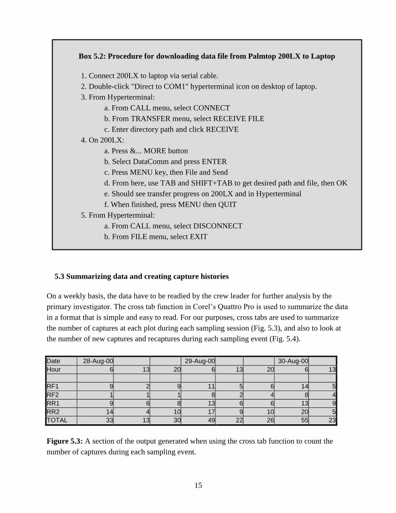
5.3 Summarizing data and creating capture histories

On a weekly basis, the data have to be readied by the crew leader for further analysis by the

primary investigator. The cross tab function in Corel‘s Quattro Pro is used to summarize the data

in a format that is simple and easy to read. For our purposes, cross tabs are used to summarize

the number of captures at each plot during each sampling session (Fig. 5.3), and also to look at

the number of new captures and recaptures during each sampling event (Fig. 5.4).

Date 28-Aug-00 29-Aug-00 30-Aug-00

Hour 6 13 20 6 13 20 6 13

RF1 9 2 9 11 5 6 14 5

RF2 1 1 1 8 2 4 8 4

RR1 9 6 8 13 6 6 13 9

RR2 14 4 10 17 9 10 20 5

TOTAL 33 13 30 49 22 26 55 23

Figure 5.3: A section of the output generated when using the cross tab function to count the

number of captures during each sampling event.

Box 5.2: Procedure for downloading data file from Palmtop 200LX to Laptop

1. Connect 200LX to laptop via serial cable.

2. Double-click "Direct to COM1" hyperterminal icon on desktop of laptop.

3. From Hyperterminal:

a. From CALL menu, select CONNECT

b. From TRANSFER menu, select RECEIVE FILE

c. Enter directory path and click RECEIVE

4. On 200LX:

a. Press &... MORE button

b. Select DataComm and press ENTER

c. Press MENU key, then File and Send

d. From here, use TAB and SHIFT+TAB to get desired path and file, then OK

e. Should see transfer progress on 200LX and in Hyperterminal

f. When finished, press MENU then QUIT

5. From Hyperterminal:

a. From CALL menu, select DISCONNECT

b. From FILE menu, select EXIT

16

28-Aug-00 29-Aug-00 TOTAL

6 13 20 6 13 20

CLRU N 20 5 7 14 1 47

R 6 5 15 25 16 20 87

MIOE N 2 1 1 4

R 5 3 5 9 5 6 33

RS 1 1 2

SOSP 1 1

TOTAL 33 13 30 49 22 26 174

Figure 5.4: A section of the output generated when using the cross tab function to count the

number of new captures and recaptures during each sampling event.

The cross tab feature can also be used to create capture histories, a complete record of when each

individual was captured throughout the course of each sampling session. Basically, the cross tab

function searches for all trapping occasions on which an individual is encountered. If the

individual was captured on a particular sampling occasion then a ―1‖ is entered into the

spreadsheet, if the animal was not captured then a ―0‖ is entered. The resulting spreadsheet can

be imported directly into the program CAPTURE for computation of abundance estimates.

Date 28-Aug-00 29-Aug-00 30-Aug-00

Hour 6 13 20 6 13 20 6 13

413905223C 1 0 1 1 0 1 0 0

41390B2117 1 0 1 1 0 0 1 1

41390D6F6D 0 0 1 1 0 0 1 0

4139181262 1 0 0 1 0 1 1 1

4139283D51 0 0 1 1 1 1 1 0

Figure 5.5: A partial capture history for five individuals (1 = capture. 0 = absent)

5.5 Calculating abundance estimates using CAPTURE

Estimating abundance by plot and session can be done in a couple different ways. Currently, we

use S-PLUS to do all our data analysis, including a call to CAPTURE. Alternatively, one could

create individual input data files and run CAPTURE manually.

17

When a trapping session is complete and the data have been verified, the raw data are imported

into S-PLUS. The working data directory is m:\splus\voles\_Data, located in the user

directory for edebevec.staff on Mercury, the Biology and Wildlife computer network. Attach to

this directory using the attach() function, or use the setup() function and choose the first

option: Small Mammal. All data from the Denali LTEM small mammal study are compiled in

the data frame allyears, currently at 25,895 rows. The 16 data fields are as follows:

Data Field Description

LOCATION * Site name (ROCK, TEK, POLY, etc.)

YEAR * Year data were collected

SESSION * Session number within year

DATE Month, day, and year that capture occurred

HOUR Trap check within day (6=0600, 13=1300, 20=2000)

PLOT Name of trapping grid or web

X X label for trap within plot

Y Y label for trap within plot

TAG Tag number of individual

TOECLIP Identifying toeclip used for part of 1992

N.R New capture (N) or recapture (R)

SPEC 4-character species identification code

SEX Sex identification (M, F)

WT Weight in grams

MORT * Logical value (T=mortality, F=not mortality)

COMMENTS Additional comments

Figure 5.6: Column names and description for small mammal capture data frame in S-PLUS.

The spreadsheet described in Figure 5.1 is imported into S-PLUS as a new data frame using the

Import Data command or by cut and pasting into an empty data sheet. The fields identified above

with an asterisk (*) are not included and need to be added with the function add.data(). It is

important to note that mortalities must be identified by the keyword ―MORT‖ in the

COMMENTS field. The letters can be any combination of upper and lower case. The data frame

that is output from add.data() can be appended onto other data frames (e.g., allyears or

denali00), or kept separate. In the past we accumulated data throughout a field season into a

single data frame, and then added the season‘s data to allyears at the end of the season. Be sure

to remember to add a column for TOECLIP before appending.

18

Other data frames within S-PLUS are used to record the dates and times that each plot is

checked. The data frame rock.sessions lists all trap checks at Rock Creek and the data.frame

other.sessions lists trap checks at all other sites. The first 4 fields in each data frame are

YEAR, SESSION, DATE, and TIME as described above for allyears. Each additional field is

for a specific plot and consists of a logical response: True if the plot was checked at that date and

time, and False if not. These data frames are needed for generating capture histories on those

occasions when there were no captures on a plot during a trap check.

These 3 data frames (allyears, rock.sessions, and other.sessions) are used to estimate

abundances using CAPTURE. The function capture.history() is used to generate capture

histories for a given year, plot, session, species, and optionally sex. Common species codes to

use are CLRU (Clethrionomys rutilis) and MISP (all Microtus species). The function

capture.history() returns a list comprised of the following objects:

Object Description

call Repeats the function call

location Site name

year Sample year

session Session number within year

plot Plot name

spec Species

sex Sex (NA if both used)

capture.history Capture history matrix (1=captured, 0=not captured)

trap.checks Date and times of all trap checks

is.mort Logical vector (T=mortality, F=not mortality)

Figure 5.7: Components of a capture history object in S-PLUS.

Once the capture history is generated, it is used with the function capture() to call the program

CAPTURE to generate the abundance estimate. By default, CAPTURE performs a model

selection routine and generates estimates under all possible models. The results of the model

selection routine are output to the S-PLUS commands window. The analyst looks over the results

and selects a model from the menu. The abundance estimate with standard error and 95%

confidence interval for the selected model are then displayed. We record the species, plot name,

session number, abundance estimate (N), standard error (SE), confidence interval, model

selected, M(t+1), and the number of mortalities. The data frames rock.estimates and

other.estimates contain abundance estimates for Rock Creek and all other sites, respectively.

19

5.6 Data archival in MS Access

At the end of each field season, data are collected and added to the MS Access database

smdata.mdb. The database consists of 6 tables and a data query form that allows for filtering the

data by year, location, plot, session, and species. Appendix 2 provides a summary of this

database. The Captures table is the equivalent of the allyears data frame in S-PLUS, containing

all the individual capture data from all years in the study. All other tables are simple

informational tables that give a general description of the locations sampled (Locations),

detailed locations of every plot (Plots), a brief schedule of plots used in each year (Plots Used),

a listing of session dates and personnel (Sessions), and vegetation surveys performed at Rock

Creek (Vegetation).

To compile the Captures table at the end of each field season, perform the following.

(a) In S-PLUS, create a temporary data frame that is the same as the seasonal data frame,

except that MORT is now 0 if false, and 1 if true. tmp <- denali00

tmp$MORT <- as.numeric(tmp$MORT)

(b) Copy this data frame into an Excel spreadsheet. Add and empty column after TAG for the

TOECLIP field. Get the last index number from the Captures table in the database.

Insert a new first column in the Excel spreadsheet that continues this index for the new

data.

(c) Save the spreadsheet as a comma-delimited file without the header row.

(d) From Access with the database open, select File > Get External Data > Import. Select the

comma-delimited file just created. Click Next a couple times. When asked ―Where would

you like to store your data?‖, select ―In an existing table‖ and choose Captures.

The Filter Data query allows you to select a subset of the data in Captures for export. You

sequentially select items from the choices on the left. Only choices that persist from one level to

the next are displayed. For example, the first selection allows your choice of year(s). As with all

selections, more than one choice can be made. Click on the year(s) you want, holding down the

Control key if selecting more than one. Then click on the right arrow to accept your choice(s).

Possible locations are then displayed in the next selection area. Choose the location(s) you are

interested in and continue until all 5 selection stages have been completed. Click on the Run

Filter button and a new table will be opened containing the requested data. You may select Save

As to save this in a file, or you can cut and paste into another application.

20

5.7 WEB presentation of data

With the 2000 field season, we began posting current information about the small mammal study

on a website. We were able to post maps and other site-specific information that the field crew

could access even before arriving in Fairbanks and we could publish abundance estimates

literally within hours of completing a session. The website homepage is currently at this address:

http://mercury.bio.uaf.edu/~edebevec.staff/denali-sites/index.html

The main page contains a map of Denali National Park and Preserve with the location of our

current 5 sampling locations. Moving the mouse over one of the sites will open a small window

containing sampling dates for the current field season. Clicking on the site will bring you to a

series of maps of increasing resolution that illustrate individual plot locations. Moving the mouse

over a plot will open another window containing latitude and longitude coordinates for the

corners. Units can be degrees/minutes/seconds or decimal degrees. Click on the Select GPS

Units button to choose. This requires writing a file to your local hard drive to specify the desired

units, so be sure you allow cookies with your browser. Additionally, there are some photographs

that can be viewed to aid in site location in the field.

Below each of the sample sites on the main map, there is an area labeled ―View Data‖. Moving

the mouse over these areas will display current plots of abundance estimates for all plots at the

site. There is also a link near the bottom of the page that brings you to another page with all

abundance estimates in tabular form.

SOP 6 — WORKING IN THE BACKCOUNTRY

6.1 Low-impact Camping

The Denali ecosystem is very fragile. Minimizing unnecessary impacts is an essential aspect of

working in the backcountry. Complications arise because trapping small mammals involves

camping in one location for 5 days and repeatedly walking the same routes to check the traps.

Walking may sound inconsequential, but minor trails can develop in only few passes across

tundra. Currently, discussions are still underway with NPS regarding how best to get the work

done while minimizing impacts. Regardless, treat the work area as sensitively as you can and

21

leave as little trace as possible. There is information and expertise available on low-impact

camping at the backcountry desk.

6.2 Bear Etiquette:

When working in the backcountry of Denali, there will be ample opportunity to view bears in

their natural habitat. This is a great privilege but a privilege that necessitates following a number

of specific rules (see below). Serious incidents are very rare but as a small mammal researcher,

additional care must be taken because some work activities may actually increase the opportunity

of having a negative bear encounter. In particular, care must be taken to properly store all bait,

mortalities, soiled nestlets, and other garbage in the Bear Resistant Food Containers (BRFCs).

This necessitates that extra space be available in your BRFCs as the amount of garbage

generated may exceed the amount of food consumed. At Rock Creek, vests and any additional

‗smelly‘ items can be stored directly in the large bear barrel. Because you will be spending more

nights in the backcountry than practically anyone else in the Park, it is particularly important not

to become complacent with respect to bears and always keep a bear safe camp. To get the full

lowdown it is also necessary to schedule a meeting with the Bear Technicians before heading

into the field. Additionally, report all unusual bear encounters to the Bear Technicians.

Figure 6.1: Obvious Low-impact Suggestions

pack out everything

make sure campsites are out of sight of the road

avoid camping in the exact same location on subsequent visits

avoid using the exact same routes repeatedly if possible

camp and cook in spots that can absorb greater impacts

do not damage vegetation unnecessarily

do not over-flag grids (amounts used will depend on vegetation cover)

explain to inquisitive backcountry users what you are doing and why

22

Figure 6.2: Preventing Bear Encounters

All food and garbage must be stored in special Bear Resistant Food Containers (BRFCs)

Cook and store food at least 100 yards from tent

Keep a clean camp

Watch for fresh tracks and scat

Avoid surprising bears

Make other loud noises to warn bears of your presence, especially in dense brush

Never intentionally approach a bear

If you encounter a bear:

DO NOT RUN! Running may elicit a chase response from an otherwise non-aggressive

bear. Bears can run faster than 30 mph (50 km/hr) – that‘s faster than you! If the bear is

unaware of you, detour quickly and quietly away.

BACK AWAY SLOWLY if the bear is aware of you but has not acted aggressively.

Speak in a low, calm voice while waving your arms slowly above your head. Bears that

stand up on their hind legs are not threatening you, but merely trying to identify you.

SHOULD A BEAR APPROACH OR CHARGE YOU, DO NOT RUN -- DO NOT

DROP YOUR PACK ! Bears occasionally make bluff charges, sometimes coming within

ten feet of a person before stopping or veering off. Dropping a pack may encourage the

bear to approach people for food. STAND STILL until the bear moves away, then slowly

back off.

IF A GRIZZLY MAKES CONTACT WITH YOU, PLAY DEAD. Curl up into a ball

with your knees tucked into your stomach, and your hands laced around the back of your

neck. Leave your pack on to protect your back.

IF A BLACK BEAR ATTACKS, fight back vigorously. Do not fight with a grizzly, play

dead.

23

6.3 Necessary Clothing:

The weather of Denali can challenge even experienced backcountry users and necessitates

adequate field clothing and gear. Technicians should be prepared for temperatures well below

zero, occasional snow at higher elevations, heavy and persistent rain, and rare sunny days with

temperatures hypothetically reaching into the nineties.

6.4 Camping Equipment

In general, camping equipment is provided by UAF but technicians may wish to use some of

their own gear (sleeping bags etc.). It is important to verify that all equipment is in good

condition prior to getting into the field. In particular, make sure the tents are seam sealed and if

Figure 6.3: Necessary Clothing (additional personal items will be added to this list) *

rubberized rain pants (goretex pants are ineffective in wet vegetation)

goretex jacket and/or rubberized rain jacket

synthetic long underwear (tops and bottoms – a second set is a good idea)

fleece jacket (warm layer)

microfleece (another layer and good to sleep in if everything else is wet)

synthetic or wool socks (several pairs)

hiking boots with good ankle support for packing heavy loads

rubber boots for day to day work in wet conditions (XtraTufs recommended)

sun hat (when the sun is out it is out for 20 hours a day)

winter toque

field pants

gloves (it is difficult to process animals wearing gloves so expect cold hands)

mosquito net (for Wonder Lake)

* As in all backcountry camping situations, there are a couple of general rules: 1)

layering clothes makes it easier to accommodate variable weather conditions, and 2)

cotton is a sponge and provides no warmth when wet (save it for the weekend).

24

they look particularly beat-up try to find a replacement. BRFCs are available from the bear

technicians or the backcountry desk.

Figure 6.4: Camping Equipment Checklist:

Four large bear resistant food containers (BRFCs) (two or three containers sufficed for

a two-person crew)

tent (ensure seems are sealed / one tent per person is required to avoid bloodshed)

sleeping pad

sleeping bag (should be rated to around 20 F)

tarps (for cooking area and UV protection for tents)

backpacks (also used for hauling traps)

topographic maps as required

stove

adequate fuel (will depend on crew size and how many coffees you drink)

pot set

bowl and utensils

mug

nalgene water bottles (two per person)

water purification system (giardia has been documented in the park)

collapsible water buckets (for hauling water to campsite)

several lighters

headlight and batteries (only needed in last weeks of field season)

suntan lotion

dish soap and scrubby

25

SOP 7 — END OF SEASON

7.1 Cleanup

All field supplies must be adequately maintained during the field season, and particular care

must be taken at the conclusion of the field season. This includes checking computers, scanners,

and Pesolas for proper functioning. All traps have to be dismantled, cleaned, and disinfected. It is

also important to make sure that all the data is ―put to bed‖. This includes providing copies of

digital photos and backup copies all data files.

7.2 Future Suggestions:

With the completion of each field season, it is very important for the field crew to provide

suggestions for the following seasons. This bottom up perspective is imperative. Of course, as is

life at the end of a long field season, many of the suggestions will sound like complaints (see

below). Of course, as is life when you manage the purse strings, the principal investigator and

NPS will nod sympathetically and then disregard many of these suggestions. Also, because these

SOPs were just written in Fall 2000, this document should be considered a first draft and any

feedback or additions would be much appreciated.

Future Suggestions from the 2000 Field Season (Cam MacDonald and Aren Eddingsaas)

The field season would be much more agreeable if the following suggestions are implemented:

1) Have a full complement of traps for each site

2) Helicopter traps into sites at beginning of year and out of sites at the end of the year (1 - 1.5

hrs of helicopter time on both ends).

These two suggestions, while expensive, would save the field crew a vast amount of work.

Hauling traps into field sites every Sunday and out every Friday took a major toll. And when

considering the number of person-days spent hauling traps across the tundra, the helicopter really

becomes a massive cost saving device.

Additionally,

26

3) Consider changing from 12 trap sessions to 10 or 11 (each session would thus end after the

0600 or 1300 check on Thursday). This would allow the crew to get out of the field at a much

more reasonable time on Thursday (1800 hrs).

4) If the above suggestions are not feasible, another layover day should be added to each

weekend to allow for modest recuperation and to prevent ‗burn-out‘.

5) Develop specific criteria for shutting down a trapping session if weather becomes difficult

(e.g., 3-inches of snow, overnight temps below 20 F, mortalities > 30% of morning captures).

6) In conjunction with NPS, determining flagging protocol and color scheme. This is of

particular importance at Polychrome, Tek 3, and Stony.

7) Having an NPS or UAF Vehicle would prevent damage to a personal vehicle on the park road.

Mileage is sufficient compensation on paved roads but not necessarily on slow, rough gravel.

8) A third person on the crew would help with the workload and potentially help with the group

―dynamics‖.

27

APPENDIX 1: SITE DESCRIPTIONS

Rock Creek (mile 3 on park road; park at C-camp): The four grids are 1.5 km north of the road at

an elevation of 2400 feet. It is an easy 20-minute walk to the site when following a trail

that follows the east ridge above Rock Creek. Two of the grids (RR1 and RR2) are

riparian and the other two (RF1 and RF2) are on the west ridge above Rock Creek.

Habitat is spruce taiga with ground vegetation including a mix of willows, grasses,

sphagnum, dwarf birch, and various berries. Because the site has been used for ten years,

there are trails between trap sites that are unsightly but facilitate trap checks. A large bear

barrel (55 gallon drum) at the campsite simplifies proper storage.

28

Teklanika (mile 26; park in pullout): The three grids are located on the eastern side of the

Teklanika River and are up to 2.5 km north of the road at an elevation of 2600 feet. It is a

45-minute traverse across scrubby tundra and numerous streams to reach the campsite.

One grid (TK3) is 15-20 minute walk south of the other two grids and this must be

negotiated 6 times a day when checking traps. Habitat for TK1 and TK2 is a mix of open

meadow and spruce taiga. TK3 is on a large river bar and is a mix of willow and scrubby

grasses.

29

Polychrome (mile 47.7; park in grader parking space on north side of road): The three grids are

located 4 km south of the highway, on the far side of the Plains of Murie and at an

elevation of 4000 feet. It is a good hour hike to the site. The best route is to thwack east

across the plains towards the river where the walking is easier. Two grids (PC1 and PC2)

are on the west side of the river and are typical alpine tundra: a scrubby mix of willows,

dwarf birch, and grasses. The third grid (PC3) is across the river and is primarily a grassy

meadow, wet on the north side. Crossing the river is generally easy in rubber boots, but

the flow is very ephemeral and heavy rains can make the crossing hazardous or even

impossible. Additionally, the elevation makes frost or snow possible at any time of the

year. The best out-of-sight campsite is tucked into a narrow canyon that cuts west into the

mountains.

30

Stony Creek (mile 65?: park in pullout just west of where Stony Creek crosses the highway): The

grids are located 4 km north of the highway, near the confluence of Stony Creek and

Little Stony Creek and at an elevation of 3500 feet. It is up to an hour and a half hike to

the site with gear. The easiest and flattest route is along the river bar. However, as at

Polychrome, the river is ephemeral and the bar can be beneath five feet of water if it has

been raining heavily. The alternate route is taking the higher, hillier route along the river

and then cutting over a ridge to the campsite. The weather can also be detrimental if 2000

is representative; the site seems to catch rain clouds sweeping across the interior and if it

is cold then expect snow. Habitat is scrubby alpine tundra and quite uniform for all three

grids.

31

Wonder Lake (mile 85; park McKinley Bar trailhead): The three grids are located 2.0km down

the McKinley Bar Trail at an elevation of 2000 feet. It is a 20-minute walk to the grids

that are only 100m off the trail. The habitat is spruce taiga / muskeg swamp. The

mosquitoes are awesome in July — bring your head net, repellent, psychiatrist, etc. As

well, take extra care to hide your tent at this site to avoid being visible from the park road

and trail.

32

APPENDIX 2: S-PLUS FUNCTIONS

add.data

DESCRIPTION

Takes raw capture data from field spreadsheet and adds required data columns

and makes necessary format changes.

USAGE

add.data(df, location, year, session, data=denali00)

REQUIRED ARGUMENTS

df data frame containing capture data from the field Lotus spreadsheet. This data

frame must have the following fields: DATE, HOUR, PLOT, X, Y, N.R, TAG, SPEC,

SEX, WT, and COMMENTS.

location character string giving the name of the location to be filled in (e.g. ―ROCK‖ or

―POLY‖).

year numeric value for the year.

session numeric value for the session.

OPTIONAL ARGUMENTS

data seasonal data frame. This data frame is only used as a reference to get the proper

order for the columns.

VALUE

The returned data frame has the following columns added: LOCATION, YEAR,

SESSION, and MORT.

DETAILS

This operation is to be performed on data from each sampling session.

EXAMPLES

> # Look at a few rows of the input data frame:

> DS6[1:5,]

DATE HOUR PLOT X Y N.R TAG SPEC SEX WT COMMENTS

2 07/17/00 6 PC2 10 F N NOT TAGGED MIMI M 13 MORT JUVE

3 07/17/00 6 PC2 6 F N 41423C760C MIMI M 32 NONSCROT

4 07/17/00 6 PC2 4 A N 41422E4759 CLRU M 14 NONSCROT

5 07/17/00 6 PC2 9 A N NOT TAGGED MIMI M 14 MORT JUVE

6 07/17/00 13 PC2 9 C ARGS

> # Now run the function:

> sc1_add.data(DS6,"STONY",2000,1)

> # Look at a few rows of the resulting data frame:

> sc1[1:5,]

LOCATION YEAR SESSION DATE HOUR PLOT X Y TAG N.R SPEC SEX WT MORT COMMENTS

2 STONY 2000 1 07/17/00 6 PC2 10 F NOT TAGGED N MIMI M 13 T MORT JUVE

3 STONY 2000 1 07/17/00 6 PC2 6 F 41423C760C N MIMI M 32 F NONSCROT

4 STONY 2000 1 07/17/00 6 PC2 4 A 41422E4759 N CLRU M 14 F NONSCROT

5 STONY 2000 1 07/17/00 6 PC2 9 A NOT TAGGED N MIMI M 14 T MORT JUVE

6 STONY 2000 1 07/17/00 13 PC2 9 C ARGS F

33

capture.history

DESCRIPTION

Returns a list that describes the capture history based on the chosen input

arguments. The output can be used as input to the function capture.

USAGE

capture.history(year, sess, plot, spec, sex, loc, df=allyears)

REQUIRED ARGUMENTS

df data frame containing capture data. This data frame must have certain fields that

correspond to the selection criteria. Required fields are LOCATION, YEAR,

SESSION, DATE, HOUR, PLOT, TAG, SPEC, SEX, MORT and are described more fully

below. Other fields likely to be included are X, Y, N.R, WT, and COMMENTS.

OPTIONAL ARGUMENTS

year vector of year(s) to be used to create the capture history. Can be entered as

numeric or character and must be in the same format as df$YEAR, currently 4

digits (1998).

sess vector of session(s) to be used in the capture history. Can be entered as numeric

or character.

plot vector of plot(s) to be used in the capture history. Must be entered as character.

Can be lower or upper case.

spec vector of species(s) for the capture history. Must be entered as character. If

"MISP" is given, then it is converted to c("MIOE","MIMI","MISP"). Can be

lower or upper case.

sex vector of sex(es) for the capture history. Must be "M" or "F".

loc vector of location(s) for the capture history. Must be entered as character. Possible

locations are "ROCK", "HINES", "CLARK", "KIKI", or "WONDER".

VALUE

The returned capture history object is a list with ten named elements.

call a listing of the command line call used to create the capture history. This is

for reference.

location character string for location (e.g. ―ROCK‖ or ―POLY‖)

year numeric year

session numeric session

plot character string for plot name(s)

spec character string for species

sex character string for sex

capture.history a column vector with an element for each individual captured as

determined by the selection criteria. Each entry is a character string of 1s

and 0s that correspond to capture and not captured, respectively. The

number of characters in the string is equal to the number of trap checks as

determined by the selection criteria.

34

trap.checks a vector with names for the trap-check occasions. The length of

trap.check equals the number of characters in the capture.history

elements.

is.mort a logical vector whose length equals the number of rows in

capture.history, corresponding to each individual captured. Value is

TRUE if the individual was a mortality and FALSE if not.

DETAILS

The following fields must be present in df and have the same spelling and

capitalization in their names.

LOCATION sampling location ("ROCK", "HINES", "CLARK", "KIKI", "WONDER", "TEK",

"POLY", or "STONY").

YEAR sampling year, with 4 digits (e.g. 1998).

SESSION sampling session. Sampling sessions for each year and each plot are numbered

from 1 to the number of sessions. This means there is no connection between

session 1 at one location and session 1 at another.

DATE sampling date in numeric format as imported from MS Excel. Can convert to

other date formats using the function dates with origin=c(12,30,1899).

HOUR sampling hour of the day. This is almost exclusively 6 (6:00AM), 13 (1:00PM), or

20 (8:00PM).

PLOT plot name. Note that the plot names uniquely identify the location, but it is useful

to have both fields.

TAG tag number.

SPEC species code.

SEX male or female.

MORT logical field. TRUE if the individual died.

When the function is run, text is output to the command window giving the total

number of individuals captured and the total number of mortalities.

EXAMPLES

> # get capture history for clethrionomys in 1998, session 5,

> # at RF1. Note location of ROCK is implied by plot name and

> # no selection is made based on sex.

> c5rf1.98 <- capture.history(1998,5,"rf1","clru")

7 Total 1 Morts

> c5rf1.98

$call:

capture.history(year = 1998, sess = 5, plot = "rf1", spec = "clru")

$location:

[1] "ROCK"

$year:

[1] 1998

$session:

[1] 5

$plot:

[1] "RF1"

$spec:

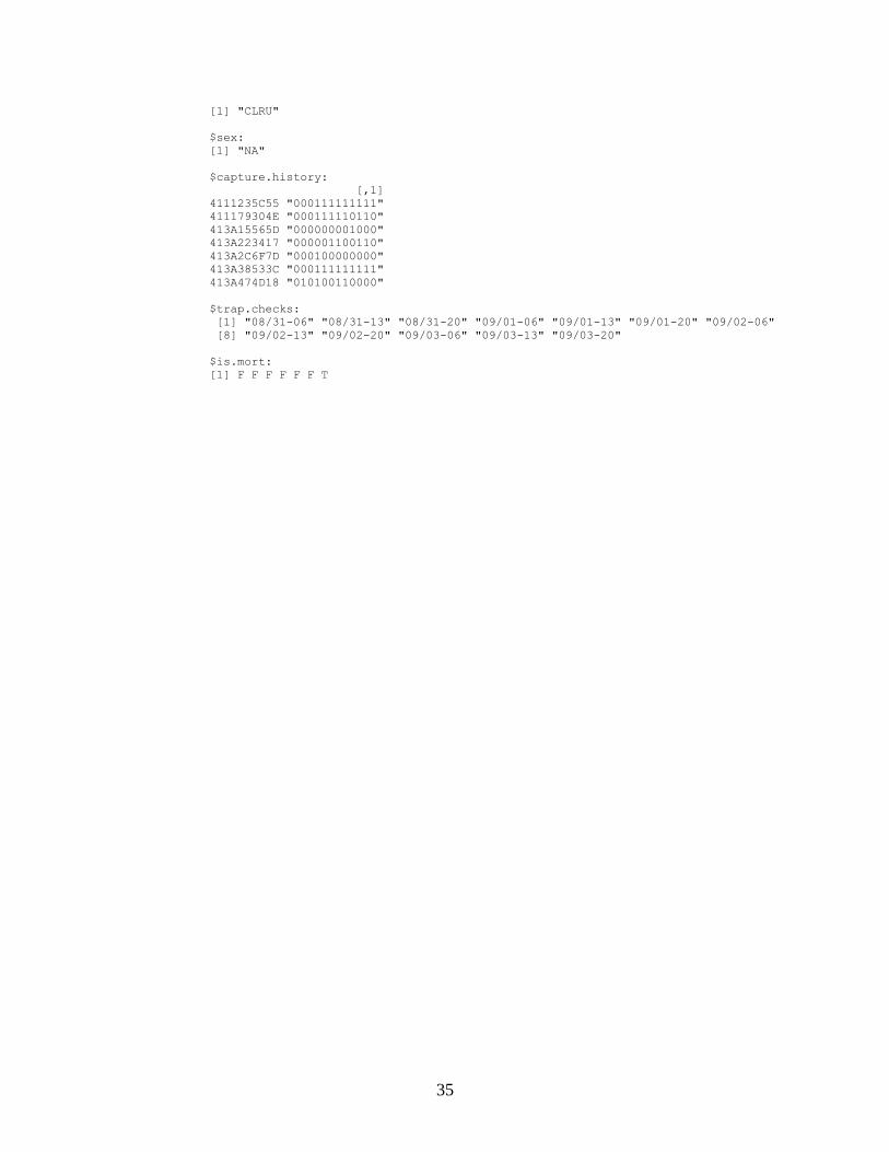
35

[1] "CLRU"

$sex:

[1] "NA"

$capture.history:

[,1]

4111235C55 "000111111111"

411179304E "000111110110"

413A15565D "000000001000"

413A223417 "000001100110"

413A2C6F7D "000100000000"

413A38533C "000111111111"

413A474D18 "010100110000"

$trap.checks:

[1] "08/31-06" "08/31-13" "08/31-20" "09/01-06" "09/01-13" "09/01-20" "09/02-06"

[8] "09/02-13" "09/02-20" "09/03-06" "09/03-13" "09/03-20"

$is.mort:

[1] F F F F F F T

36

capture

DESCRIPTION

Creates an ASCII input file from the input capture history, runs the program

CAPTURE.EXE, and displays selected results.

USAGE

capture(cap.hist, title, infile, outfile, path,

exepath="c:\\capture", remove.morts=T, remove.zeros=F,

remove.unknowns=F, record=NULL, only.once=F)

REQUIRED ARGUMENTS

cap.hist capture history object as created by a call to the function capture.history.

OPTIONAL ARGUMENTS

title a title to be printed in the CAPTURE output file. If missing, "Untitled

Capture Analysis" is used.

infile root filename for the CAPTURE input file to be created. The extension .inp

will be appended. If missing, the name of cap.hist will be used.

outfile root filename for the CAPTURE output file. The extension .out will be

appended. If missing, the same root filename as infile will be used.

exepath path for the CAPTURE executable file.

path path for infile and outfile. If missing, exepath will be used.

remove.morts logical. If TRUE, mortalities as identified in cap.hist$is.mort will be

removed from the capture history. The number of mortalities removed will

be printed prior to any abundance estimates in the output.

remove.zeros logical. If TRUE, trap checks where no individual were captured are

removed.

remove.unknowns logical. If capture.history encounters individuals with missing tag

numbers, tag values of "unknown1", "unknown2", etc., are generated. If

remove.unknowns is TRUE, then these individuals are removed from the

analysis.

record name for S-PLUS data frame object to be created or appended to with

selected results from a CAPTURE analysis.

only.once logical. If TRUE, results from only one model will be displayed. Used to

save time when the user simply wants to view the model results selected as

appropriate by CAPTURE.

SIDE-EFFECTS

A text file is created by S-PLUS and saved in path. The program CAPTURE.EXE is

run and generates an output text file that is saved in the same directory.

VALUE

Results from CAPTURE are displayed on the screen. If a name is given for record,

then selected results will be appended to an existing data frame of that name or to

a new data frame with that name. The data frame contains the following fields:

37

LOCATION, YEAR, SESSION, PLOT, SPEC, SEX, NMORTS, REM.MORTS, UNKNOWN,

REM.UNKNOWN, REM.ZEROS, N, SE, LO95, HI95, M, MODEL

DETAILS

The input file for CAPTURE is automatically generated and run. CAPTURE

performs three tasks: (1) closure test, (2) model selection, and (3) estimation using

all models. When completed, summary statistics are displayed along with results

from the closure test and model selection. A menu is then displayed where the

user can select a model for which results will be displayed. The nine possible

models are M(o), M(h), M(b), M(t), M(bh), M(th), M(tb), Chao's M(t), and Chao's

M(h). The results for the selected model are displayed and the menu again

appears. The user quits the function by selecting 0 at the menu. If only.once is

set to TRUE, then the user can only select a single model for viewing. This is

useful if the user always wants to only view results for the "appropriate" model,

saving keystrokes if several analyses are to be run consecutively.

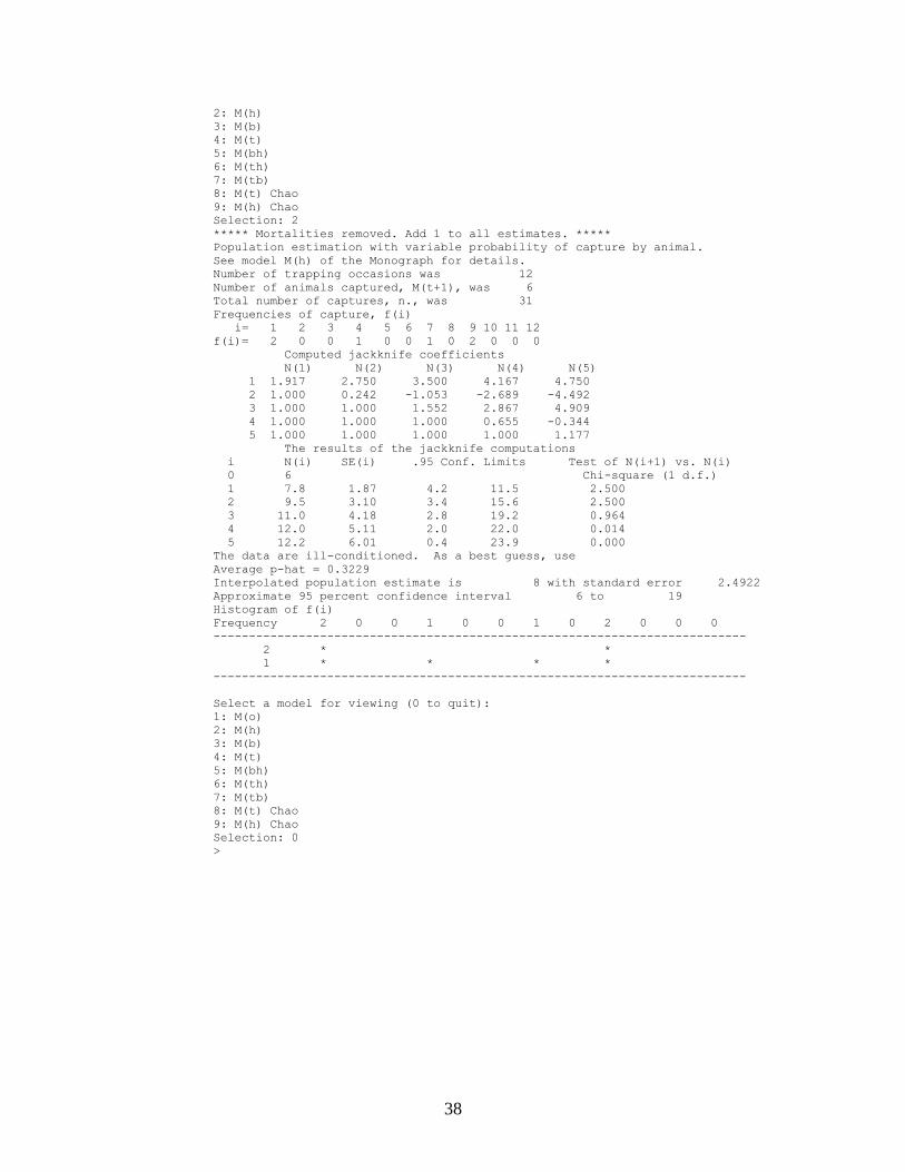
EXAMPLES

> capture(c5rf1.98,"1998 Clethrionomys RF1 Session 5","c5rf198")

From output file c:\capture\c5rf198.out

*** Mortalities removed ***

Summary of captures read

Number of trapping occasions 12

Number of animals captured 6

Test for closure

z-value -3.302

Probability of a smaller value 0.00048

Model selection procedure

Occasion j= 1 2 3 4 5 6 7 8 9 10 11 12

Animals caught n(j)= 0 0 0 4 3 4 4 3 3 4 4 2

Total caught M(j)= 0 0 0 0 4 4 5 5 5 6 6 6

6

Newly caught u(j)= 0 0 0 4 0 1 0 0 1 0 0 0

Frequencies f(j)= 2 0 0 1 0 0 1 0 2 0 0 0

Test for heterogeneity of trapping probabilities in population.

M(o) vs M(h) Expected values too small. Test not performed.

Test for behavioral response after initial capture.

M(o) vs M(b) X^2 = 9.037 df = 1 p = 0.00265

Test for time specific variation in trapping probabilities.

M(o) vs M(t) X^2 = 3.115 df = 11 p = 0.98911

Goodness of fit test of model M(h)

M(h) vs not M(h) X^2 = 28.538 df = 11 p = 0.00268

Goodness of fit test of model M(b)

M(b) vs not M(b) X^2 = 26.173 df = 9 p = 0.00192

Contribution of first capture homogeneity across time

X^2 = 21.735 df = 2 p = 2e-005

Contribution of recapture homogeneity across time

X^2 = 4.438 df = 7 p = 0.72814

Goodness of fit test of model M(t)

M(t) vs not M(t) Expected values too small. Test not performed.

Test for behavioral response in presence of heterogeneity.

M(h) vs M(bh) Expected values too small. Test not performed.

Model selection criteria. Model selected has maximum value.

Model M(o) M(h) M(b) M(bh) M(t) M(th) M(tb) M(tbh)

Criteria 0.95 1.00 0.75 0.75 0.00 0.41 0.92 0.77

Appropriate model probably is M(h)

Suggested estimator is jackknife.

Select a model for viewing (0 to quit):

1: M(o)

38

2: M(h)

3: M(b)

4: M(t)

5: M(bh)

6: M(th)

7: M(tb)

8: M(t) Chao

9: M(h) Chao

Selection: 2

***** Mortalities removed. Add 1 to all estimates. *****

Population estimation with variable probability of capture by animal.

See model M(h) of the Monograph for details.

Number of trapping occasions was 12

Number of animals captured, M(t+1), was 6

Total number of captures, n., was 31

Frequencies of capture, f(i)

i= 1 2 3 4 5 6 7 8 9 10 11 12

f(i)= 2 0 0 1 0 0 1 0 2 0 0 0

Computed jackknife coefficients

N(1) N(2) N(3) N(4) N(5)

1 1.917 2.750 3.500 4.167 4.750

2 1.000 0.242 -1.053 -2.689 -4.492

3 1.000 1.000 1.552 2.867 4.909

4 1.000 1.000 1.000 0.655 -0.344

5 1.000 1.000 1.000 1.000 1.177

The results of the jackknife computations

i N(i) SE(i) .95 Conf. Limits Test of N(i+1) vs. N(i)

0 6 Chi-square (1 d.f.)

1 7.8 1.87 4.2 11.5 2.500

2 9.5 3.10 3.4 15.6 2.500

3 11.0 4.18 2.8 19.2 0.964

4 12.0 5.11 2.0 22.0 0.014

5 12.2 6.01 0.4 23.9 0.000

The data are ill-conditioned. As a best guess, use

Average p-hat = 0.3229

Interpolated population estimate is 8 with standard error 2.4922

Approximate 95 percent confidence interval 6 to 19

Histogram of f(i)

Frequency 2 0 0 1 0 0 1 0 2 0 0 0

---------------------------------------------------------------------------

2 * *

1 * * * *

---------------------------------------------------------------------------

Select a model for viewing (0 to quit):

1: M(o)

2: M(h)

3: M(b)

4: M(t)

5: M(bh)

6: M(th)

7: M(tb)

8: M(t) Chao

9: M(h) Chao

Selection: 0

>

39

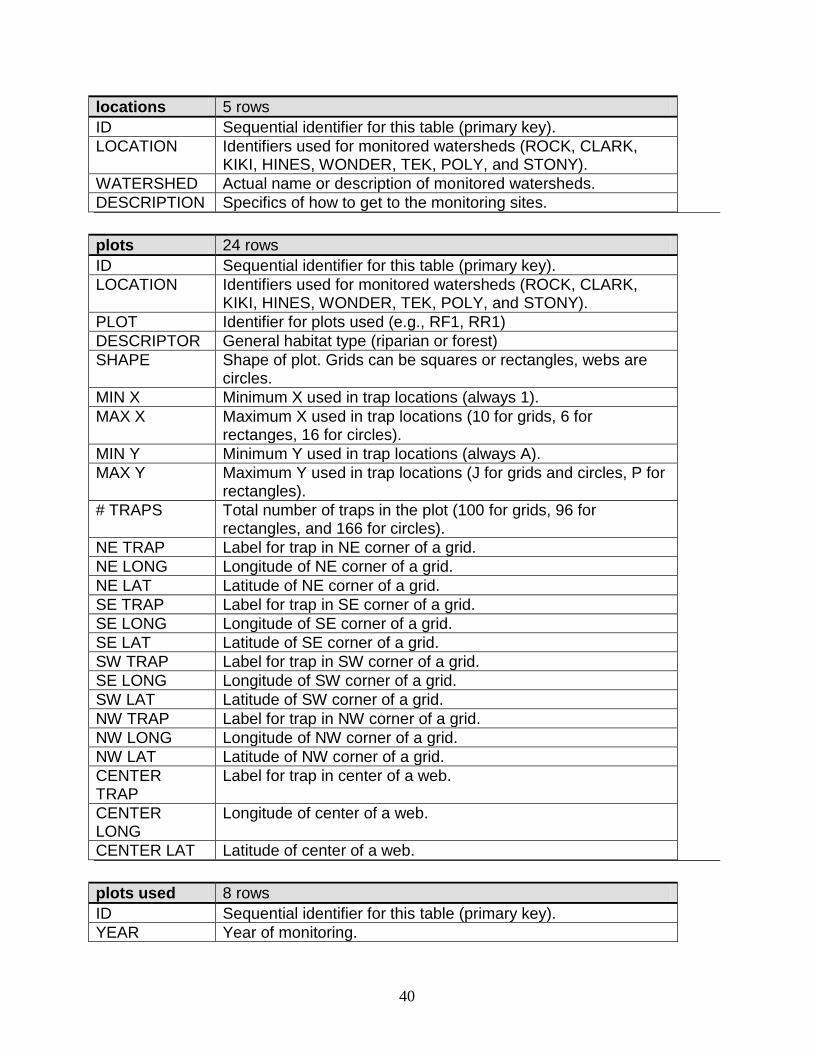
APPENDIX 3: SMALL MAMMAL DATABASE

Filename: smdata.mdb

Format: MS Access 97

Tables: captures locations plots plots used sessions vegetation

Queries: Get Data Unique Locations Unique Plots Unique Sessions Unique Years Unique Species

Forms: Filter Data Filter Help

TABLES

captures 25,895 rows

ID Sequential identifier for this table (primary key).

LOCATION Identifiers used for monitored watersheds (ROCK, CLARK, KIKI, HINES, WONDER, TEK, POLY, and STONY).

YEAR Year of monitoring

SESSION Identifier for primary sampling events at each location.

DATE Date of sampling.

HOUR Hour of day when sampling occurred.

PLOT Identifier for plots used (e.g., RF1, RR1)

X Row identifier for traps in grids or radial identifier for traps in webs.

Y Column identifier for traps in grids or spoke identifier for traps in webs.

TAG Unique mark applied to each animal (PIT tag number).

TOECLIP Toeclip identifier applied to some animals in 1992.

STATUS New capture (N) or recapture (R)

SPEC Species of animal captured.

SEX Sex of animal captured.

WT Weight of animal captured.

MORT Identifies whether the animal died (True/False)

COMMENTS Comments entered by field crew.

40

locations 5 rows



WATERSHED Actual name or description of monitored watersheds.

DESCRIPTION Specifics of how to get to the monitoring sites.

plots 24 rows




DESCRIPTOR General habitat type (riparian or forest)

SHAPE Shape of plot. Grids can be squares or rectangles, webs are circles.

MIN X Minimum X used in trap locations (always 1).

MAX X Maximum X used in trap locations (10 for grids, 6 for rectanges, 16 for circles).

MIN Y Minimum Y used in trap locations (always A).

MAX Y Maximum Y used in trap locations (J for grids and circles, P for rectangles).

# TRAPS Total number of traps in the plot (100 for grids, 96 for rectangles, and 166 for circles).

NE TRAP Label for trap in NE corner of a grid.

NE LONG Longitude of NE corner of a grid.

NE LAT Latitude of NE corner of a grid.

SE TRAP Label for trap in SE corner of a grid.

SE LONG Longitude of SE corner of a grid.

SE LAT Latitude of SE corner of a grid.

SW TRAP Label for trap in SW corner of a grid.

SE LONG Longitude of SW corner of a grid.

SW LAT Latitude of SW corner of a grid.

NW TRAP Label for trap in NW corner of a grid.

NW LONG Longitude of NW corner of a grid.

NW LAT Latitude of NW corner of a grid.

CENTER TRAP

Label for trap in center of a web.

CENTER LONG

Longitude of center of a web.

CENTER LAT Latitude of center of a web.

plots used 8 rows


YEAR Year of monitoring.

41

FU Sampling done on plot FU (True/False)

RF1 Sampling done on plot RF1 (True/False)

RF2 Sampling done on plot RF2 (True/False)

RR1 Sampling done on plot RR1 (True/False)

RR2 Sampling done on plot RR2 (True/False)

FWE Sampling done on plot FWE (True/False)

FWW Sampling done on plot FWW (True/False)

RW Sampling done on plot RW (True/False)

CF1 Sampling done on plot CF1 (True/False)

CF2 Sampling done on plot CF2 (True/False)

NCF2 Sampling done on plot NCF2 (True/False)

CR1 Sampling done on plot CR1 (True/False)

CR2 Sampling done on plot CR2 (True/False)

HF1 Sampling done on plot HF1 (True/False)

HF2 Sampling done on plot HF2 (True/False)

HR1 Sampling done on plot HR1 (True/False)

HR2 Sampling done on plot HR2 (True/False)

KF1 Sampling done on plot KF1 (True/False)

KF2 Sampling done on plot KF2 (True/False)

KR1 Sampling done on plot KR1 (True/False)

KR2 Sampling done on plot KR2 (True/False)

WL Sampling done on plot WL (True/False)

WL1 Sampling done on plot WL1 (True/False)



TK1 Sampling done on plot TK1 (True/False)



PC1 Sampling done on plot PC1 (True/False)



SC1 Sampling done on plot SC1 (True/False)



sessions 53 rows




SESSION Identifier for primary sampling events at each location.

START Start date for each session.

END End date for each session.

PERSONNEL Field personnel for each session.

42

vegetation 72 rows




TRANSECT Identifier for each 20 m transect in a plot.

LAYER Identifies understory (UNDER) or overstory (OVER)

0CM Vegetation at start of transect.

50CM Vegetation at 50 cm along transect.





































43




Queries Get Data Query designed for use with the Filter Data form.

Unique Locations

Query designed for use with the Filter Data form.

Unique Plots Query designed for use with the Filter Data form.

Unique Sessions

Query designed for use with the Filter Data form.

Unique Years Query designed for use with the Filter Data form.

Unique Species Query designed for use with the Filter Data form.

Forms Filter Data Used to filter capture data by year, location, plot, session, and

species.

Filter Help Instructions for using Filter Data. Used separately or from Filter Data form.

long-term ecological monitoring protocol for small …

Documents