long-term evaluation of the hydro-thermodynamic soil ...molders/jgr_2006.pdfscheme’s frozen...

Long-term evaluation of the Hydro-Thermodynamic Soil-Vegetation

Scheme’s frozen ground/permafrost component using observations at

Barrow, Alaska

Nicole Molders and Vladimir E. RomanovskyGeophysical Institute, University of Alaska Fairbanks, Fairbanks, Alaska, USA

Received 8 March 2005; revised 23 September 2005; accepted 28 October 2005; published 28 February 2006.

[1] The multi-layer frozen ground/permafrost component of the hydro-thermodynamicsoil-vegetation scheme (HTSVS) was evaluated by means of permafrost observations atBarrow, Alaska. HTSVS was driven by pressure, wind, air temperature, specific humidity,snow-depth, rain, downward shortwave and long-wave radiation observations for 14consecutive years. Observed soil temperature data are available at various times duringthis period. HTSVS predicts soil temperatures that are slightly too low with root meansquare errors (RMSEs) of, on average, less than 3.2 K. Sensitivity studies suggest that thetreatment of snow and vegetation cover may be reasons for the inaccuracy. HTSVS’original thermal conductivity parameterization provides thermal conductivity values thatare too high compared to typical observations. Introducing a parameterization frequentlyused in the permafrost research community, which was modified for application innumerical weather prediction (NWP) and climate models and model consistency inHTSVS, improves soil temperature predictions and reduces RMSEs in some layers by upto 1 K, and on average by 0.2 K. Assuming five to ten layers for the first 2 or 3 m as isusually done in NWP and climate modeling is insufficient to capture the active layerdepth, because the number and position of the grid nodes play a role. The depth of thelower boundary of the soil model and the boundary condition affect the overallperformance. Consequently, under current computational possibilities, simulatingpermafrost and the active layer in atmospheric models requires a compromise between thedegree of accuracy and affordable computational time.

Citation: Molders, N., and V. E. Romanovsky (2006), Long-term evaluation of the Hydro-Thermodynamic Soil-Vegetation

Scheme’s frozen ground/permafrost component using observations at Barrow, Alaska, J. Geophys. Res., 111, D04105,

doi:10.1029/2005JD005957.

1. Introduction

[2] At high latitudes, permafrost, soil in which temper-atures remain below 0�C for at least two consecutive years,and the active layer, which thaws seasonally, are the primarysubsurface components of the land-atmosphere system. Theassociated thermal and hydrological conditions affect cli-mate by the exchange of heat, moisture, and matter [e.g.,Stendel and Christensen, 2002; Molders and Walsh, 2004].At the same time, permafrost temperature and stability andactive layer depth are sensitive to climatic change [e.g.,Kane et al., 1991]. Atmospheric warming may start perma-frost warming, and change the long-term mean surfacetemperature with feedbacks to climate and other potentialimpacts. Permafrost thawing, for instance, can cause hugeeconomic and infrastructure damages and ecosystemchanges, and affects trace gas and water cycles [Esch andOsterkamp, 1990; Cherkauer and Lettenmaier, 1999;Oechel et al., 2000; Serreze et al., 2000; Romanovsky andOsterkamp, 2001; Zhuang et al., 2001]. To appropriately

describe heat, moisture, and matter exchange at the surface-atmosphere interface in the Arctic and to examine perma-frost-climate feedbacks, modern climate models requiresuitable land-surface models (LSMs) to simulate frozenground and permafrost dynamics.[3] In recent decades geologists and geophysicists have

exerted great effort to develop site-specific permafrostmodels to examine permafrost dynamics [e.g., Goodrich,1982; Nelson and Outcalt, 1987; Kane et al., 1991;Romanovsky and Osterkamp, 1997; Smith and Riseborough,2001; Zhuang et al., 2001; Ling and Zhang, 2003].Detailed permafrost models (1) usually require a largeamount of computational time because of their fine verticalresolution (�0.05 m), (2) typically run at large time stepsdue to geologically slow processes, (3) are site-specific,and (4) have to be calibrated [e.g., Romanovsky et al.,1997; Osterkamp and Romanovsky, 1999; Romanovsky andOsterkamp, 2001]. In calibration, a great part of a data setis used to determine optimal soil-transfer parameters,leaving a lesser part for model evaluation.[4] Applying a typical calibration technique certainly

would lead to better predictions than those presented here.

JOURNAL OF GEOPHYSICAL RESEARCH, VOL. 111, D04105, doi:10.1029/2005JD005957, 2006

Copyright 2006 by the American Geophysical Union.0148-0227/06/2005JD005957$09.00

D04105 1 of 16

However, climate prediction with calibrated LSMs or cou-pling calibrated permafrost models to climate models wouldrequire consistent soil temperature data for calibration on aglobal scale. Since as of today no such data set exists, usageof calibrated permafrost models in climate models is tech-nically impossible. Therefore, and since calibration coeffi-cients may be climate sensitive, the climate-modelingcommunity does not use calibration techniques in modelsthat are applied in climate-system modeling. In addition,permafrost and climate models are not coupled becauseclimate simulations require input of water and energy fluxesto the atmosphere at time steps of several minutes or so.Thus, a vertically highly-resolved permafrost model wouldhave to run with this much smaller time-step makingsynchronous simulations by a climate model coupled witha permafrost model computationally prohibitive.[5] Apparently high-latitude terrestrial processes, espe-

cially those related to permafrost variations, have yet toreceive a concerted effort within the context of globalclimate modeling. Studies carried out with the standaloneversions of 21 state-of-the-art LSMs using soil temperatureobservations along with fluxes and snow data from the18-year Valdai data set, collected at a site without perma-frost but with regularly frozen ground in winter, showed thatexplicit inclusion of soil-water freezing improves simula-tions of soil temperature and its variability at seasonal andinter-annual scales [Luo et al., 2003]. For all these reasonspermafrost, permafrost dynamics, and soil-water freezing/thawing must be considered in climate assessment.[6] To achieve this goal, knowledge and well-accepted

concepts from permafrost and atmospheric sciences can becombined to build a suitable soil model for use in climateand Arctic numerical weather prediction (NWP) models.Recently,Molders et al. [2003a] developed a frozen ground/permafrost component for the HTSVS [Kramm et al., 1994,1996] for simulating soil processes including freezing andthawing and soil-heat conduction in NWP and climatemodels. In the present study, we evaluate HTSVS’ perfor-mance in simulating the dynamics associated with perma-frost and the active layer by using long-term soil-temperatureobservations made at Barrow, Alaska (USA), a site with coldpermafrost conditions.

2. Method

2.1. Brief Model Description

[7] HTSVS [e.g., Kramm et al., 1994, 1996; Molders etal., 2003a; Molders and Walsh, 2004] describes the ex-change of momentum, heat, and moisture at the vegetation-soil-atmosphere interface, with special consideration givento the heterogeneity on the micro-scale by the Deardorff-type mixture approach, i.e., a grid cell can be partly coveredby vegetation [Deardorff, 1978; Kramm et al., 1996]. Itconsiders snow’s insulating effect and retardation of infil-tration by a multi-layer snow model, water uptake by plantsincluding a vertically variable vegetation-type dependentroot distribution, and the temporal variation of soil albedoand snow albedo and emissivity. In addition to mineralsoils, HTSVS can consider organic soil layers (e.g., moss,lichen, peat) [Molders and Walsh, 2004] that are of specialrelevance for the moisture distribution within soils andpermafrost dynamics [e.g., Beringer et al., 2001].

[8] The multi-layer soil model considers the (vertical)heat- and water-transfer processes (including the Richardsequation) [Kramm et al., 1994, 1996], and soil freezing/thawing [Molders et al., 2003a] based on the principles ofthe linear thermodynamics of irreversible processes [e.g., deGroot, 1951; Prigogine, 1961]. The governing balanceequations for heat and moisture including phase transitionprocesses and water extraction by roots c are [e.g., Philipand de Vries, 1957; de Vries, 1958; Sasamori, 1970;Flerchinger and Saxton, 1989; Kramm et al., 1994, 1996;Molders et al., 2003a],

C@TS

@t¼ @

@zSl@TS

@zS

� �þ @

@zSLvrwDT;v

@TS

@zS

� �

þ @

@zSLvrwDh;v

@h@zS

� �þ Lf rice

@hice@t

ð1Þ

@h@t

¼ @

@zSDh;v

@h@zS

� �þ @

@zSDh;w

@h@zS

� �

þ @

@zSDT;v

@TS

@zS

� �þ @Kw

@zS� crw

� ricerw

@hice@t

ð2Þ

Here zS, l, Lv, Lf, TS, h, hice, Dh,v, Dh,w and DT,v are soildepth, thermal conductivity, latent heat of condensation andfreezing, soil temperature, volumetric water and ice content,and the transfer coefficients for water vapor, water, andheat. Soil hydraulic conductivity Kw = ks W

2b+3 dependson the saturated hydraulic conductivity, ks, the relativevolumetric water content W = h/hs, porosity hs and pore-size distribution index b [e.g., Clapp and Hornberger, 1978;Dingman, 1994]. The volumetric heat capacity of moist soil[Molders et al., 2003a]

C ¼ 1� hsð ÞrScS þ hrwcw þ hicericecice þ hs � h� hiceð Þracpð3Þ

is a function of the density rS, rw, rice, and ra and specific heatcapacity cS, cw, cice, and cp of the dry soil material, water, iceand air. The thermal conductivity of unfrozen grounddepends on water potential y = ys W

�b [McCumber, 1980]

l ¼419 exp � Pf þ 2:7ð Þð Þ Pf < 5:1

0:172 Pf � 5:1

8<: ð4Þ

with ys being the saturated water potential and Pf =2 + 10 log jyj. At soil temperatures below 0�C, a mass-weighted thermal conductivity depending on volumetricice and water content is calculated using equation (4) forthe liquid and 2.31 J/(msK) for the solid phase. Thetransfer coefficients are given by [Philip and de Vries,1957; Kramm, 1995]

Dh;v ¼ �anDwbhs � h

hrdrw

gyRdTS

ð5Þ

Dh;w ¼ � bksys

hhhs

� �bþ3

ð6Þ

DT;v ¼ anDw hs � hð Þ rdrw

Lv � gyRdTS

2ð7Þ

D04105 MOLDERS AND ROMANOVSKY: EVALUATION OF HTSVS FOR PERMAFROST

2 of 16

D04105

where g is the acceleration due to gravity, a, n, Dw, rd, andRd are the torsion factor that considers curvatures in the soilmaterial due to roots [Sasamori, 1970; Zdunkowski et al.,1975; Sievers et al., 1983; Kramm et al., 1996], a correctionfactor that is typically close to 1 and hence assumed to be 1,the molecular diffusion coefficient of water vapor in moistair, and the density and gas constant for dry air.[9] At a given soil temperature below 0�C all water in

excess of [Flerchinger and Saxton, 1989]

hmax ¼ hsLf TS � 273:15ð Þ

gysTS

� ��1=b

ð8Þ

is frozen (Figure 1).[10] In equation (1), the first term on the right side

describes soil temperature changes by divergence of soil-heat fluxes. The second term represents the divergence ofsoil-heat fluxes due to water-vapor transfer. The third termdescribes how a soil moisture gradient contributes to thesoil-temperature change (Dufour effect), and the last termaddresses soil temperature changes due to freezing/thawing.In equation (2), the first two terms on the right siderepresent the changes in volumetric water content causedby divergence of water vapor and water fluxes. The thirdterm describes how a temperature gradient contributes to thechange in volumetric water content (Ludwig-Soret effect).The saturation vapor pressure depends on soil temperature.Thus, a gradient in soil temperature leads to differences insaturation pressure and a water vapor flux that affects soilmoisture. This phenomenon, well known to occur in snow,also exists in soils [Philip and de Vries, 1957; de Vries,1958]. The fourth term represents changes due to hydraulicconductivity, the fifth gives water uptake by roots, and thelast considers changes due to freezing/thawing. The Ludwig-Soret and Dufour effects are cross-phenomena usually con-sidered in the thermodynamics of irreversible processes.[11] The number of model layers can be arbitrarily

chosen. In the reference simulation (CTR), the uppermostsoil-layer ranges from the Earth’s surface to the uppermostlevel within the soil at 0.01 m depth. Between that level andlowest level at 20m depth, all 20 layers are spaced by thesame logarithmic increment so that central differences canbe used in solving the coupled equations (1) and (2) by ageneralized Crank-Nicholson scheme. In this configurationsoil-layer boundaries are at approximately 0, 0.01, 0.015,0.02, 0.03, 0.05, 0.07, 0.11, 0.16, 0.25, 0.37, 0.55, 0.82,1.22, 1.81, 2.71, 4.04, 6.02, 8.99, 13.41, and 20 m depth. Ifnot mentioned differently, soil temperature and relativevolumetric water and ice content are held constant at�9.5�C, 0.06, and 0.817 m3 m�3 at the lower boundary ofthe soil model at 20 m depth throughout the entire simulationtime in accordance with observations [Romanovsky et al.,2002]. This grid and these boundary conditions are used in thereference simulation.[12] HTSVS calculates snow albedo asnow in accord with

Luijting et al. [2004] and Molders et al. [2003a] forreference height air temperature TR below and above thefreezing point

Here v is wind speed, and tsnow is the time after the lastsnow event. Luijting et al.’s formula was derived from dailyaverages of downward and upward shortwave radiationmeasured between 2001 and 2002 at the AtmosphericRadiation Measurement (ARM) program [Ellingson et al.,1999] site. Molders et al.’s formula was derived from datameasured by the U.S. Army Corps of Engineers [1956] inthe contiguous United States in the 1950’s (see Molders etal. [2003a] for details).

2.2. Site Description

[13] The permafrost site at Barrow (71�180N, 156�470W,5m a.s.l.) is located in fairly flat and sodden terrain, withcontinuous cold permafrost and numerous thaw lakes. Theuppermost 0.2 m thick soil layer consists of silt with tracesof organic material. Underneath this mixed layer a layer ofpure silt is located that reaches to 2 m depth. Below 2 mdepth, a 10 m thick layer follows made up of a mixture ofsand, gravel and some silt. Silt with some sand occurs from12 to 34 m depth. The soil physical parameters (Table 1)used in this study are derived from the quantities determinedby inverse solution modeling [Osterkamp and Romanovsky,1997]. The freeze-thaw characteristic curves at variousdepths as obtained by using the parameters of Table 1 inequation (8) normalized with porosity (Figure 1) hardlydiffer from the freeze-thaw curves derived for this site byRomanovsky and Osterkamp [2000] using variations in soiltemperature within the active layer and near-surface perma-frost.[14] Barrow has an Arctic climate. For the last climate

period (1971–2000), the annual mean wind speed was

asnow tð Þ ¼0:63þ 0:0011TR þ 0:01hs � 0:009vþ 4:492 10�7tsnow for TR < 273:15K

0:35þ 0:18 exp�tsnow

114048

� �þ 0:31 exp

�tsnow

954720

� �for TR � 273:15K:

8><>: ð9Þ

Figure 1. Dependence of freeze-thaw characteristic curveat various depths as obtained by equation (8) normalizedwith the porosity derived from the Barrow soil analysis onsoil temperature and relative volumetric water content (W =h=hs ). Relative volumetric water content is dimensionless.


3 of 16

D04105

7.6 m/s; it is generally windy, with fall being the windiestseason. On average, annual mean air temperature is �12�C.Generally, February is the coldest (�26.6�C) and July thewarmest month (4.7�C). Air temperatures remain below0�C through most of the year, with daily maxima exceeding0�C on 109 days per year. Annual average precipitationamounts to 105 mm, of which on average 74 mm falls assnow year round. Transition from snow to snow-free con-ditions occurs in late May/early June. Barrow receives nosunlight between 18 November and 24 January, and con-stant sunlight between 10 May and 2 August.

2.3. Soil Temperature Data

[15] Daily averages of soil temperature are available for18 August 1993 to 9 August 1996, and 21 August 1998 to17 August 1999 at 0.01, 0.08, 0.15, 0.22, 0.29, 0.55, 0.75,and 1 m depth [Hinkel et al., 2001]. Hourly measurementsare available at the surface, 0.04, 0.1, 0.17, 0.24, 0.32, 0.4,0.47, 0.55, 0.7, 0.85, and 1.08 m for 11 August 20020900 UT to 11 August 2003 0800 UT from the BarrowPermafrost Observatory of the International Arctic ResearchCenter [e.g., Yoshikawa et al., 2004]. Soil temperaturemeasurements have an accuracy of ±0.5K. Since sensibleand latent heat flux or runoff are of marginal interest forpermafrost scientists, these quantities were not measured atthe Barrow Permafrost Observatory.

2.4. Forcing Data

[16] Forcing data are available from 1 January 1990 to 31December 2003. Observed wind, air and dew point temper-atures, and pressure data are taken from the Barrow ClimateMonitoring and Diagnostics Laboratory (CMDL) site. TheCMDL site is 11 m above sea level, and was 100 m and1 km away from the permafrost site for data recorded in the90’s and from 2000 onwards, respectively. Note that thepermafrost site was moved in 2000. Air and dew pointtemperatures were measured in aspirated sun shields at 2 mheight. Missing data were linearly interpolated. Specifichumidity was derived from dew-point temperature using thepsychrometer formula.[17] Precipitation amount was measured with an unheated

tipping bucket rain gauge; i.e., no solid precipitation wasreported at the permafrost site. Due to the large snowfallcatch deficiencies [e.g., Yang and Woo, 1999; Yang et al.,2000; Sugiura and Yang, 2003], and because no snowfalldata were available at the permafrost sites, we droveHTSVS with snow depth measured at the Barrow CMDLsite and used only observed liquid precipitation. To ensurethat snow depth only changes when a change in snow depthwas reported, we determined snow density according toequation (9) in Molders and Walsh [2004]. We did not

explicitly calculate compaction, settling and melt-waterpercolation as usually performed by HTSVS, because theseprocesses would alter snow depth in HTSVS’ originalformulation. When no change in snow depth was reported,but outflow and/or sublimation were predicted by HTSVS,snow density was reduced in the simulation for continuityreasons to ensure conservation of water (hs rs = rw hw wherehs and hw are snow depth and height of snow waterequivalent). Because of this necessity, snow density couldnot be used for calculation of snow thermal conductivity;instead we used a constant value of 0.14 W/(Km) [Lee,1978]. When a new snowpack was reported, initial snowdensity was treated in accord with Molders and Walsh[2004].[18] Radiation data are taken from the Barrow ARM site,

which is at the same location as the CMDL site. Down-welling shortwave radiation was measured at 1-min intervalsby an unshaded pyranometer with a hemispheric field of viewand an inverted Eppley Laboratory, Inc., Precision SpectralPyranometer (PSP). This instrument measures in a nominalwavelength range of 0.3–2.8 micrometers with a responsetime, sensitivity, and uncertainty of 1-s, �9 mV/Wm�2, and±3% or 10Wm�2, respectively. Short-wave radiation may beunderestimated during snow events and snow blow as theseevents cover the radiometer with snow.[19] Down-welling long-wave radiation is measured be-

tween 40 and 50 micrometers by a shaded pyrgeometer withhemispheric field of view. Downward long-wave radiationdata are available as 3-min averages until 12/31/1997 and as1-min averages since 1/1/1998. Occasionally missing datawere substituted by downward long-wave radiation calcu-lated in accord with Eppel et al. [1995]. Since no data oncloud fraction were available, we assumed an averagecloudiness of 80% in parameterization of downward long-wave radiation. Thus, calculated downward long-waveradiation will be under/overestimated for more/less than80% cloud fraction.

2.5. Meteorological Conditions

[20] During our episode, annual average downward short-wave and long-wave radiation, air temperature, and windspeed were 96.9 Wm�2, 224 Wm�2, �11.5�C, and 5.7m/s,respectively. This period was slightly warmer (0.5 K) andcalmer (1.9 m/s) than the 1971–2000 average.[21] The episode 2002/03 was the warmest and 1994/95

the coldest (Table 2); the average air temperatures of1993/94, 1995/96, and 1998/99 hardly differ. The meanspecific humidity differs only slightly for the first fourobservational episodes (0.004 g/kg at maximum), while thatfor 2002/03 is 0.01 g/kg higher than that for the driest episode(1994/95). This results from the fact that warmer air can take

Table 1. Soil Parameters as Used in the Simulations for Barrowa

Depth, m Material hs, m3 m�3 cs rs, 10

6J/(m3K) b, -.- ks, 10�6m/s ys, m ls, W/(mK)

0–0.2 silt with organics 0.6 0.85086 2.545 1.134 �0.389 1.04970.2–1 silt 0.55 0.971071 2.6875 2.493 �0.396 0.75361–2 silt 0.55 0.971071 2.6875 1.869 �0.396 0.97912–12 sand, gravel, some silt 0.55 0.971071 2.6 141.000 �0.030 0.937612–34 silt and some sand 0.44 1.159974 2.85 91.620 �0.405 0.6137aThe letters hs, csrs, b, ks, ys, and ls stand for porosity, dry soil volumetric heat capacity, pore-size distribution index, saturated hydraulic conductivity,

saturated water potential, and thermal conductivity of the dry soil material, respectively.


4 of 16

D04105

up more water vapor than relatively colder air before satura-tion occurs. Averaged snow depth was about 8% higher in1993/94 and 2002/03, and about 8% lower in 1998/99 than in1994/95 or 1995/96. The number of days with reported snowdepth strongly differs for our observational episodes (Table2). Averaged mean wind speed was about the same for theepisodes 1994/95, 1995/96, and 1998/99, while it was appre-ciably higher in 1993/94 and 2002/03. Average insolationdiffers by up to 6Wm�2 between the observational episodes.Annual accumulated rain was more than 8% higher in 1993/94 and 1998/1999 than for the other observational episodes.

2.6. Initialization

[22] The model was started using a climatologic soiltemperature profile and assuming that all pores are filledwith water and/or ice. HTSVS was forced by 1990 data,repeating that year three times to reach equilibrium betweensoil temperatures, volumetric water and ice content andclimate (model spin-up). Soil temperatures predicted for thethird repeated year hardly (<0.001 K) differ from the secondyear’s temperatures. The second and first year’s soil temper-atures differ by 0.5 K (0.1, 0.05, 0.01, 0.005 K) after 1 day(77, 137, 199, 210 days) of the second year. Since thedifferences between the first and the second year are alreadyless than 0.5 K after 1 day, we conclude that the modelresponds well to the atmospheric forcing, and that it quicklyachieves an acceptable equilibrium between soil and atmo-sphere. The 0.5 K discrepancy is of the same magnitude asthe error typical for routine soil temperature measurements.We use the soil temperature, volumetric water and icecontent, snow temperature and density obtained at the endof this three year spin-up as initial conditions for thesimulations that continuously run from 1 January 1990 to31 December 2003. Note that soil temperature resultsobtained without the spin-up hardly differ from thosepresented here.

2.7. Evaluation

[23] HTSVS was driven by hourly averages of wind, airtemperature, specific humidity, pressure, rain, snow depth,and downward shortwave and long-wave radiation. Dailyaverages of simulated and observed soil temperatures werecompared for various depths. We performed sensitivitystudies on vertical grid resolution, assumptions and simpli-fications typically made in NWP and climate modeling, andparameterizations to (1) assess their impact on the modeloutcome, and (2) identify model deficits and limitations ofpredictability.[24] Systematic and non-systematic errors contribute to

the prediction error. To quantify the model errors we

calculate the bias

�f ¼ 1

n

Xni¼1

fi ð10Þ

root-mean-square error

RMSE ¼ 1

n� 1

Xni¼1

fið Þ2 !1=2

ð11Þ

and the standard deviation of error

SDE ¼ 1

n� 1

Xni¼1

fi � �f� 2 !1=2

ð12Þ

Here fi is the difference between the ith predicted andobserved soil temperature and n is the total number ofobservations. The bias represents systematic errors fromconsistent misrepresentation of geometrical, physical, ornumerical factors, while SDE represents random errorscaused by uncertainty in initial and boundary conditions orobservations. RMSE evaluates overall performance andprevents positive and negative errors from cancelling eachother out.

3. Results

3.1. General Remarks

[25] Temperature and moisture states evolve by fluxeswhich themselves depend on those states [Entekhabi andBrubaker, 1995]. Thus, false predictions of soil temperatureand moisture profiles can produce incorrect phase transitionprocesses and soil-heat and moisture fluxes that propagatein incorrect water and energy fluxes to the atmosphere, andhence limit the reliability of NWP or climate models.Therefore a soil model has to be evaluated at varioustemporal scales for a wide range of climate conditions.Evaluation of HTSVS by data on mean values of windspeed, temperature, and humidity, and on eddy flux densi-ties (the so-called eddy fluxes) of momentum, sensible heat,and water vapor gathered during the Great Plains Turbu-lence Project, GREIV I-1974 (GREnzschicht InstrumentelleVermessung phase I, i.e., first phase of probing the atmo-spheric boundary layer) [e.g., Kramm, 1995], SANA(SANierung der Atmosphare uber den neuen Bundeslander,i.e., recovery of the atmosphere over the new federalcountries) [e.g., Spindler et al., 1996], CASES97 (Cooper-ative Atmosphere Surface Exchange Study 1997) [e.g.,

Table 2. Averages of Atmospheric Conditions for the Five Observational Episodesa

Episode

AirTemperature,

�CSpecific

Humidity, g/kgWind

Speed, m/sSnow

Depth, mmDownward ShortwaveRadiation, W m�2

Downward Long-WaveRadiation, W m�2

Number ofSnow-Cover Days, -.-

1993/94 �11.1 0.225 6.20 142 96.4 271.1 1671994/95 �12.9 0.224 5.31 129 93.1 247.3 1861995/96 �11.1 0.226 5.33 138 92.3 237.4 2041998/99 �11.0 0.228 5.11 123 98.6 238.7 2212002/03 �9.8 0.234 5.88 143 96.7 252.7 183

aNote that averages are calculated for the observational episodes and not for hydrological years.


5 of 16

D04105

LeMone et al., 2000] and BALTEX (BALTic sea EXperi-ment) [e.g., Raschke et al., 1998] showed that HTSVSaccurately simulates the diurnal course of state variablesand fluxes [Kramm, 1995; Molders, 2000; Narapusetty andMolders, 2005]. By using lysimeter data from a midlatitudesite with occasionally frozen ground in winterMolders et al.[2003a, 2003b] found that HTSVS predicts the long-term(2050 days) accumulated sums of evapotranspiration andrecharge with better than 15% accuracy. Soil temperatureswere predicted within 1–2 K accuracy, on average [Molderset al., 2003b].[26] The suitability for long-term integration can only be

evaluated using routine data because sophisticated fieldexperiments cannot be performed continuously over years.Due to logistic difficulties routine data are often lessaccurate than data collected in special field experimentswhere scientists stand by to immediately fix problems (e.g.,remove snow from the radiometer, replace failing parts,check data logger). Field experiments are usually designedfor a particular evaluation or to answer a question; allrequired model data are measured and quantities are ratherover- than underdetermined. When using routine data oftensome data needed as model input or forcing are unavailableor not available with sufficient resolution. Consequently,evaluations based on routine data will never yield results asgood as those based on data from a good field experiment[e.g., Spindler et al., 1996; Slater et al., 1998; Molders etal., 2003b].

3.2. Systematic Errors and Overall Performance

[27] Since rain data are only available as daily accumu-lated values, hydrological and energetic consequences of theunknown temporal evolution of rain may cause discrepan-cies between simulated and observed soil temperature. Theconsequences for soil moisture and runoff have been dis-cussed elsewhere [e.g., Molders and Raabe, 1997; Molderset al., 1999]. Inaccurately measured rain due to catchdeficiencies or traces of rain and great snowfall spatial

variability known for Arctic regions and Barrow may causesimilar errors.[28] Except for some sensitivity studies HTSVS has a

cold bias (Table 3). There are several reasons: (1) In nature,snow thermal conductivity depends on snow density andtemperature [Sturm et al., 1997], while we used a constantvalue (0.14 W/(mK)) for the reasons outlined in section 2.4.Therefore snow-heat fluxes (counted positive when down-ward) toward the soil will be overestimated if natural thermalconductivity is higher than the model value, and vice versa.This uncertainty is unavoidable as no measurements of snowthermal conductivity were available. (2) During snow eventsand snow blow, measured long-wave radiation values maybe too small if the radiometer is snow-covered. Thesemeasurement errors in the forcing data cause systematicerrors in predicted soil temperature toward colder values (seeSDE in Table 3). (3) Water vapor may deposit onto radio-meters as frost leading to underestimation of downwardlong-wave radiation that finally contributes to the cold bias.Note that 50Wm�2 average lower downward long-waveradiation can lead to a doubling of the frequency of dayswith soil temperatures below 0�C, an underestimation of soiltemperature, and an overestimation of frost depth [Molderset al., 2003b] in midlatitude winter.[29] On average, HTSVS simulates onset of thaw-up and

freeze-up about 13 and 5 days too early (Table 3). Sensi-tivity to simulation setup is marginal; ±1 day for thaw-up,±3 days for freeze-up. Average onset of thaw-up is 31, 8, 8,15, and 3 days, and of freeze-up 4, 3, 10, 5, and 3 days tooearly for 1994, 1995, 1996, 1999, and 2003, respectively(e.g., Figure 2). There are several reasons for prematurethaw-up: (1) Incorrect snow depth forcing may greatlycontribute to premature thawing. As pointed out, snowdepth was measured 100 m (1990’s) and 1000 m (2000onwards) away from the permafrost site. The snow depthsite is 6 m higher than the permafrost site, so snow easilygets blown away, while it deposits at the permafrost site.Snow-depth reports usually stop when snow cover becomes

Table 3. Statistics on Model Performancea

RMSE, K Bias, K SDE, K F-Statistic Significance r Offset of Thaw-Up, d Offset of Freeze-Up, d

CTR 3.2 �1.3 2.9 1.099 0.168 0.933 �13.2 �5.0CTR-EQ4 3.4 �0.1 3.4 1.067 0.020 0.908 �13.2 �5.2S10-3 4.0 �2.6 3.1 1.100 0.003 0.931 �13.0 �4.2S10-2 3.4 �1.7 3.0 1.075 0.008 0.930 �13.2 �5.0S10-20 3.1 �1.2 2.8 1.074 0.189 0.936 �13.0 �4.4SHOM 3.4 �1.3 3.1 1.170 0.035 0.925 �13.2 �5.4SB3L10 2.8 0.1 2.8 1.103 0.166 0.937 �13.2 �4.8SB2L10 3.1 �0.5 3.0 1.065 0.060 0.930 �13.4 �4.2SB3L5 3.2 �0.3 3.2 1.175 <0.001 0.931 �13.4 �4.4SNWTHC 4.0 �2.3 3.3 1.151 <0.001 0.926 �13.2 �5.6SNWHS 3.1 �1.0 3.0 1.128 0.003 0.930 �13.0 �5.2S5SNL 3.3 �1.3 3.0 1.047 0.209 0.929 �13.0 �5.6SALB 3.2 �1.9 2.6 1.025 0.274 0.946 �13.0 �5.2

aRMSE, bias, standard deviation error SDE, F-statistic, significance, and Pearson correlation coefficient r are calculated over all depths and the entiretime for which soil temperature observations are available. The F-statistic and significance calculation refer to the success of HTSVS to predict the sametime series of temperature variations. Simulations with statistically significant (at the 90% or higher confidence level) different temporal evolution are givenin bold. The mean offset (simulated-observed) for onset of thawing and freezing is given for the uppermost soil layer and averaged over all seasons forwhich observational data are available. CTR, S10-3, S10-2, S10-20 refer to the reference simulation, the simulations with a lower boundary at 20 m depthand 10 layers in the uppermost 3, 2 and 20 m, respectively; S5-3 has five layers to 3 m depth. SHOM assumes the same soil properties throughout thecolumn. CTR-EQ4 uses equation (4) for thermal conductivity. SB3L10 and SB2L10 have 10 layers and the bottom of the soil model at 3 and 2 m depth.SB3L5 has five layers and the bottom of the soil model at 3 m depth. SALB uses Molders et al.’s [2003a] snow albedo parameterization. S5SNL considersfive instead of three snow model layers. SNWTHC uses 0.42 W/(mK) as snow thermal conductivity, SNWHS assumes a 10% increase in snow depth.


6 of 16

D04105

Figure 2


7 of 16

D04105

patchy; therefore there may be still snow at the permafrostsite although snow-depth reports indicate none. Advancingsnow cover disappearance by 10 days can increase maxi-mum soil temperature up to 6.6, 2.2, 1.5, and 0.7 K andannual means by 0.2, 0.2, 0.1, and 0.1 K at the surface, 0.5,1, and 2 m depth [Ling and Zhang, 2003]. These values arewithin the range of our discrepancies. (2) The urban effectmay accelerate snowmelt [Hinkel et al., 2003] at the snow-depth site as compared to the permafrost site farther awayfrom town. (3) At Barrow, trace precipitation varies spatiallyand occurs with high frequency [e.g., Yang and Woo, 1999;Sugiura and Yang, 2003]. Thus, the systematic errors ofgauge-measured rain include not only wind-induced under-catch, wetting, and evaporation losses, but also trace rainloss [cf. Sugiura and Yang, 2003]. (4) A fixed vegetationalbedo (as usually applied in NWP andmany climate models)and the snow albedo parameterization may contribute todiscrepancies.[30] Reasons for premature freeze-up include: (1) Non-

reported snow (depth). Ling and Zhang [2003] reported thatdelaying the snow-cover onset date by ten days can result in adecrease in maximum soil temperature up to 9, 2.9, 2, and1.1 K and in annual average temperature up to 0.7, 0.5, 0.4,and 0.4 K at the surface, 0.5, 1, and 2 m depth. These valuesare within the range of our discrepancies. (2) Problems withthe downward long-wave radiation measurements andreplacing missing values by calculated ones may contributeto premature active layer freezing. Note that Slater et al.[1998] reported premature freezing of up to 2 months forthe Best Approximation for Surface Exchange scheme

[Desborough, 1997], related to the parameterization ofdownward long-wave radiation; Molders et al. [2003a]reported that the frequency of predicted days with frozenground is very sensitive to the parameterization of downwardlong-wave radiation. Schlosser et al. [2000] and Molders etal. [2003a] also found that the water budget was sensitive tothe parameterization of downward long-wave radiation.[31] Generally, annual averages of RMSEs and SDEs are

higher in 1998/99 than for 1993 to 1996, and 2002/03,respectively, which may be due to problems with the newradiation equipment deployed in 1998. In 1998/99 muchmore missing data had to be replaced by calculations thanfor other time periods.[32] Soil moisture measurements are available at 0.10,

0.22, and 0.35 m depth for 2002/03. During this time thegroundwater table is around 0.1 m in early summer indicatingsaturated soil at all soil moisture sensors. Above 0.1 m,predicted volumetric water content of the thawed active layerdecreases in summer and refills in fall. As expected forpermafrost soils [Hinkel et al., 2001], predicted total relativesoil moisture content equals or is close to 1 all year round.

3.3. Soil Thermal Conductivity

[33] Predicted soil temperature is highly sensitive to thethermal conductivity of the ground and snow [e.g., Zhang etal., 1996; Riseborough, 2002]. The parameterization ofthermal conductivity according to equation (4) providesmuch higher thermal conductivity values (Figure 3) thantypically observed in permafrost soils (e.g., Table 4).Moreover, equation (4) provides a decrease of thermalconductivity as the ground freezes, while typically theopposite is observed (e.g., Table 4). Therefore, we replacedequation (4), which is frequently used in the LSMs ofatmospheric models, by Farouki’s [1981] parameterization,l = ls

(1�hs) lw(hs�hice) lice

hice, which is often applied inpermafrost modeling [e.g., Lachenbruch et al., 1982;Riseborough, 2002]. Here ls (see Table 1 for values),lw(=0.57 W/(mK)), and lice(=2.31 W/(mK)) are thermalconductivity of dry soil, water, and ice, respectively. Wemodified this parameterization for model-consistent appli-cation in HTSVS as:

l ¼ l 1�hsð Þs lh

wlhiceice l

hs�h�hiceð Þa ð13Þ

where la(=0.025 W/(mK)) is the thermal conductivity of air.Farouki’s formulation neglects the impact of air becausepermafrost soil pores are typically totally ice-filled. Weconsider the effect of partly air-filled pores for two reasons:First, consistency with equations (1) to (3) requires inclusionof air, because these equations explicitly consider watervapor fluxes (third and first on the right side of equations (1)and (2), respectively) and air (last term of equation (3)).Second, a LSM for use in NWP and climate models mustalso describe non-permafrost, partly air-filled soils appro-

Figure 2. Simulated and observed soil temperatures for (a) 1993–1996, (b) 1998/99, and (c) 2002/03 and simulated andobserved vertical soil temperature profiles at various seasons for (d) 1993/94, (e) 1994/95, (f) 1995/96, (g) 1998/99, and(h) 2002/03 as obtained by the reference simulation (CTR). CTR uses equation (13) to calculate thermal conductivity.The x-axis in (a), (b), and (c) differ, (a) shows about three years worth of data, (b) and (c) show one freeze-thaw cycle. They-axis in (d) to (h) differ, because soil temperature measurements were available at eight levels to 1 m depth in the 1990’sand at 12 levels up to 1.10 m depth in 2002/03.

Figure 3. Thermal conductivity as obtained byequations (4) and (13). Figures for other soil layers showthe same basic pattern.


8 of 16

D04105

priately (e.g., in midlatitudes or deserts). Permafrost soils areusually saturated, i.e., hair = hs � h � hice = 0, meaning hs �hice = h, and la

(hs�h�hice) = la0 = 1, and equation (13) and

Farouki’s equation provide identical results.[34] The HTSVS original formulation generally pro-

vides greater thermal conductivity values than the newparameterizations (Figure 3). For our episode thermalconductivity calculated with equation (4) ranges between0.292 and 5.745 W/(mK); on average, values are about2.2 W/(mK) and 1.5 W/(mK) in the deeper and uppersoil respectively, much higher than values typically mea-sured at Barrow (Table 4). The simulation carried outwith equation (13) provided thermal conductivity valuesbetween 0.149 (uppermost layer after dry episode) and1.52 W/(mK); on average, values are about 1.1 W/(mK)between 0.25 and 1.8 m and less than 1 W/(mK) elsewhere,and lower in summer than winter. These values agree wellwith the range previously determined for frozen andthawed Barrow soil (Table 4). Note that in an uncertaintyanalysis using Gaussian error propagating techniques,Molders et al. [2005] identified equation (4) as criticalbecause the natural variance in empirical parameters (pore-size distribution index, saturated water potential, porosity)propagates to great uncertainty in calculated thermal con-ductivity. Uncertainty in equation (13) parameters propa-gates less strongly leading to less parameter-causedstatistical uncertainty in calculated thermal conductivity,soil temperatures, and soil-heat fluxes.[35] Averaged over all depths, RMSEs are about 3.0 K,

4.8 K and 3.1 K for 1993/96, 1998/99 and 2002/03, in thesimulation performed with equation (4). This simulation isdenoted CTR-EQ4 hereafter. In the simulation usingequation (13), called CTR further on, RMSEs decreasedby up to 0.4, 0.2, and 0.2 K on average for 1993–1996,1998/99, and 2002/03, respectively; by up to 1 K in somelayers; and overall by on average 0.2 K (Table 3). Activelayer depth is overestimated (up to 0.5 m) in CTR-EQ4,and underestimated (up to 0.3 m) in CTR (see Figures 2and 4).[36] In CTR-EQ4, the variance of simulated and observed

soil temperature time series differs significantly (at the 95%or higher confidence level) overall (Table 3) and below0.3 m for all except the last episode. Statistically significantdifferences only occur for a short time between 0.3 and0.7 m in CTR. The discrepancies for the latter can beexplained by the difficulty in capturing the actual activelayer depth on a non-regular grid.[37] Based on these findings equation (13) should be

favored for calculation of thermal conductivity. Therefore,in the following simulations, we use equation (13) and refer

Table 4. Soil Thermal Conductivity Determined for Barrow for

Thawed and Frozen Soila

Depth, m

Soil Thermal Conductivity

Thawed Ground, W/(mK) Frozen Ground, W/(mK)

0–0.2 0.7 1.40.2–1 1.0 1.81–2 0.95 1.62–12 1.6 2.412–34 1.2 1.9aUpdated data from Romanovsky and Osterkamp [2000].

Figure 4. Simulated and observed soil temperatures asobtained by CTR-EQ4 for (a) 1993–1996, (b) 1998/99, and(c) 2002/03. CTR-EQ4 uses equation (4) instead ofequation (13) to calculate thermal conductivity.


9 of 16

D04105

to the simulation with equation (13) as the referencesimulation (CTR).

3.4. Reference Simulation (CTR)

[38] In the reference simulation, soil temperatures andtheir annual variance are captured better between 0.2 m and0.3 m and below 0.7 m beneath the surface than elsewhere.Annual RMSEs are highest in the uppermost 0.1 m becausevariability is greater close beneath the surface than deeperin the soil and hence is more difficult to predict [cf.Molders et al., 2003b]. Moreover, the possibility that thetemperature field is influenced by sensor installation ishigher close beneath the surface than deeper in the soil.Discrepancies in variance at depths between 0.3 and 0.7 mare due to incorrect prediction of the active layer depth(Figure 2). Around 1 m depth, soil hydraulic propertieschange (Table 1), which may contribute to the largeRMSEs found here. Uncertainty in the empirical soilphysical parameters for gravel causes discrepancies thatpropagate to the 1 m depth level leading to RMSEs up to6.8 K at 1.08 m depth in 2002/03. Averaged over alldepths, RMSEs are about 2.6, 4.6, and 2.9 K for 1993/96,1998/99 and 2002/03, respectively.[39] The model tends to underestimate soil temperatures

slightly in winter of 1993/94, 1995/96, and 1998/99, andin late winter of 1994/95 (Figure 2). Early winter soiltemperatures are too high in 1994/95. Factors contributingto this deficiency are non-matching thermal conductivity ofthe snow, and errors in measured long-wave downwardradiation.[40] Predicted soil temperatures are too low in all five

summers and falls. The depth of the active layer isusually underestimated (up to 0.3 m) in midsummer.However, the predicted temperature state of the activelayer gradually improves close beneath the surface inmidsummer (Figure 2). On average, the location of thefreezing line is broadly captured during summer withinthe range of what the grid resolution permits.[41] The model does not capture the zero-curtain situation

(i.e., a layer of unfrozen ground between two layers offrozen ground) between 0.1 and 0.25 m that is observed infall. Note that this zero curtain situation lasts for anextremely long time in fall 1998 (Figure 2). The reasonsgiven in section 3.2, the vertically coarse resolution (only 12layers below 1 m depth) and active layer depth underesti-mation contribute to this failure.[42] Below the active layer, the seasonal cycle of soil

temperature is acceptably captured for all five years of data(Figure 2). In 1998/99, predicted soil temperatures are toolow throughout the year except for spring.

3.5. Vertical Resolution

[43] In theory, fine soil grid resolution guarantees accuratesimulation of soil temperature and moisture profiles. How-ever, global data sets describing vertical distributions of soilparameters and initial soil temperature and moisture condi-tions must be available at the same resolution. Thus, avail-ability of these data sets and the huge computational burdenassociated with a fine grid limit the vertical grid resolutionthat can be reasonably chosen in NWP or climate models.Consequently, the balance between efficiency and practicalaccuracy dictates the resolution of soil grids in the LSMs of

these models and limits accuracy of soil-temperature predic-tions. Currently, most of these models use five to ten soillayers [e.g., Bonan et al., 2002; Stendel and Christensen,2002] that cover a depth down to 2 to 3 m [e.g., Chen andDudhia, 2001; Molders and Walsh, 2004].[44] We examine the impact of the vertical grid resolution

to (1) assess the current representation of soil processes inNWP and climate modeling, and (2) recommend an opti-mum for currently available computational possibilities. Toaccomplish this we perform simulations using ten layers tocover the first 2, 3, and 20 m beneath the surface, referredto as S10-2, S10-3, and S10-20, respectively. Like CTRthese runs are performed with a constant soil temperature of�9.5�C at 20 m depth to minimize the impact of the soilmodel’s lower boundary. For S10-2 and S10-3, this proce-dure permits non-constant fluxes, soil temperatures andmoisture at 2 and 3 m depth, respectively.3.5.1. Soil Grid[45] To produce ten layers in the upper 3 m, the model is

run with 13 layers (reaching to about 0.01, 0.02, 0.04, 0.07,0.13, 0.24, 0.45, 0.84, 1.59, 2.99, 5.63, 10.62, and 20 m).Due to the coarser resolution soil temperature profilespredicted by S10-3 show fewer details, and on averageRMSEs 0.3, 0.4, and 0.2 K higher for 1993–1996, 1998/98and 2002/03 than those obtained by CTR (Figures 2 and 5).Compared to CTR, S10-3 captures freezing and thawingand the related release and consumption of heat less well.The variance of the predicted and observed soil temperaturetime series differs significantly (Table 3), mainly between0.3 and 0.7 m depth in 1993–1996.[46] To produce ten layers in the upper 2 m or so, the

model is run with 14 layers (reaching to about 0.01, 0.02,0.03, 0.06, 0.1, 0.19, 0.33, 0.6, 1.07, 1.93, 3.46, 6.21, 11.15,and 20 m). Thus, S10-2 permits more details than S10-3, butless than CTR. Again the coarser resolution reduces predic-tion accuracy leading to average RMSEs 0.9, 1, and 0.9 Khigher than CTR for 1993–1996, 1998/98 and 2002/03.Simulated soil conditions are too warm in late winter andspring 1994, and too cold in late winter 1995, all winter1995/96 and 1998/1999, fall 2002, and all summers. Thevariance of simulated and observed soil temperatures differssignificantly in the first 0.3 m beneath the surface.[47] Using ten layers to a depth of 20 m (reaching to

about 0.01, 0.02, 0.05, 0.13, 0.29, 0.68, 1.59, 3.69, 8.60,and 20 m) affects the RMSE slightly. Occasionally thevariance of simulated and observed soil temperaturediffers significantly between 0.3 and 0.7 m depth in1993–1996 and below 0.7 m in 2002/03, but not onaverage (Table 3).[48] Evidently, the number and position of the grid nodes

play a role in capturing the active layer depth. This fact isalso manifested by the change in bias (Table 3). Discrep-ancies of 0.2 to 1 K between simulations and observationscan be caused by grid resolution with impact on thesimulated temperature variation. The findings imply that acompromise between the number of grid layers and thedepth of the lower soil model boundary on one side and theamount of computational time on the other has to be made,which is easier on a logarithmic grid than on the equallyspaced grid typically used in permafrost modeling. Interest-ingly, the impact of a coarse resolution in the deep soillevels is on average higher in winter than summer.


10 of 16

D04105

3.5.2. Soil Characteristics Profile[49] Most modern soil models used in atmospheric NWP

or climate models assume one soil type for the entire soilcolumn [e.g., Slater et al., 1998; Schlosser et al., 2000]. To

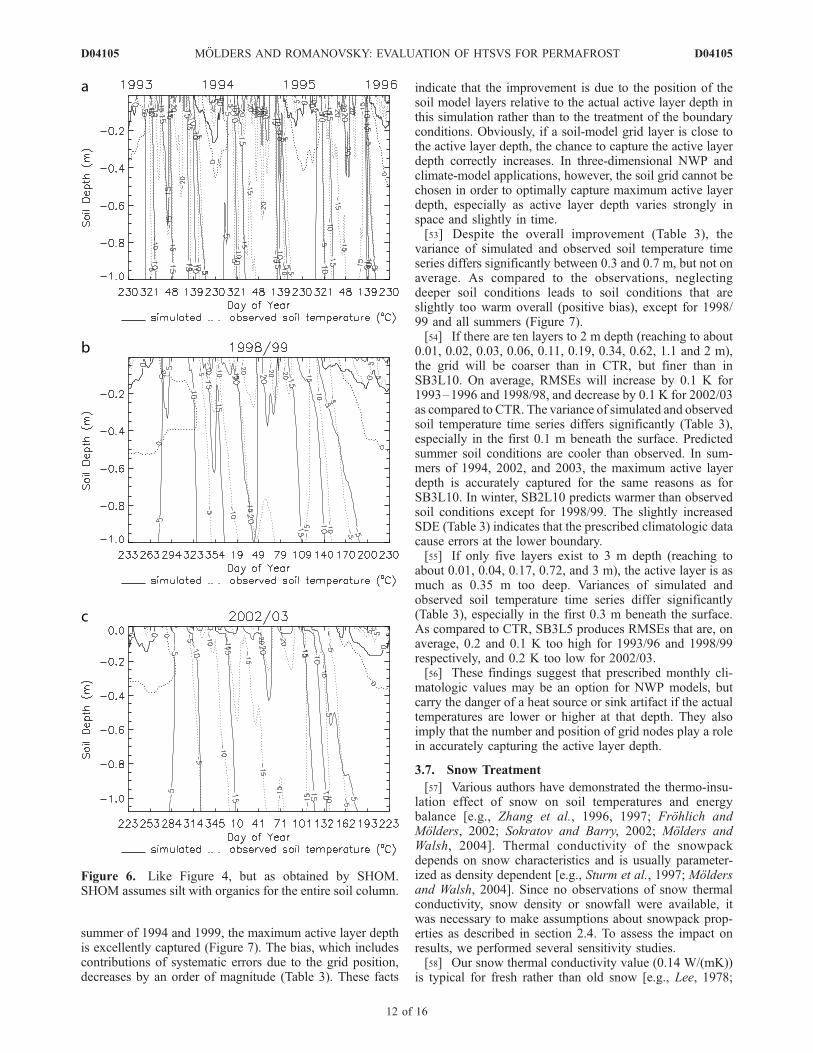
examine the impact of this assumption, a sensitivity study(SHOM) was performed wherein the parameters of theuppermost soil layer were used for the entire soil column.The simulated soil temperature pattern misses many detailsthat result from the vertical profile of soil parameters(Figures 2 and 6). As compared to CTR, and even in theuppermost layer where the soil type remained the same,RMSEs increased on average by 0.1, 0.4, and 0.3 K for1993–1996, 1998/99 and 2002/03. The variance of simu-lated and observed soil temperature time series differssignificantly (Table 3). While for 1993–1996 soil temper-atures close beneath the surface are too high during winter,they are too low in the winters of 1998/99 and 2002/2003.Summer soil temperatures that are too low lead to anunderestimation of the active layer depth (up to 0.4 m).

3.6. Lower Boundary

[50] Ideally, the bottom of a soil model is placed at a levelof constant soil temperature and moisture states as in ourreference run at 20 m depth. Most modern soil models usedin NWP or climate models typically set their lower bound-ary around 2 or 3 m depth [e.g., Chen and Dudhia, 2001;Molders and Walsh, 2004]. In permafrost soils, however,seasonal and decadal variations in soil temperature existeven below 15 m depth [Romanovsky et al., 1997]. Thus,using a constant soil temperature at the bottom of a soilmodel at 2 or 3m depth is generally impractical in climatemodeling, as it introduces artificial sources and sinks forheat and moisture [e.g., Stendel and Christensen, 2002]. Forthe typical forecast range of NWP (several days) a constantlower boundary condition can be suitable if appropriatelyset [e.g., Narapusetty and Molders, 2005]. Typically, NWPmodels use a prescribed fixed climatologic temperature,which varies monthly and spatially, as a lower boundarycondition. In contrast, climate models usually assume zero-flux conditions at the lower boundary of the soil model[Oleson et al., 2004]. However, zero heat and moisture fluxmust not necessarily exist at 2 or 3 m depths [e.g., Zhang etal., 1996; Romanovsky et al., 1997; Molders et al., 2003a,2003b].[51] Sensitivity studies, called SB2L10 and SB3L10

hereafter, were carried out with ten layers wherein the lowerboundary condition varied according to a climatologicannual course at 2 and 3 m depth. A further simulation,SB3L5, used five layers and climatologic data at 3 m depth.Note that for climate change scenarios climatologic valuescannot be used as a lower boundary condition because theymay alter with climate.[52] If there are ten layers in the upper 3 m (reaching to

about 0.01, 0.02, 0.04, 0.07, 0.13, 0.24, 0.45, 0.84, 1.59 and3 m), the grid will be coarser than that of CTR in the first3 m beneath the surface. As evidenced by the RMSEs, bias,and SDEs (Table 3), changing the position of grid nodesalso affects how accurately different soil layer character-istics can be resolved. In SB3L10, RMSEs decrease onaverage by 0.1, 0.7, and 0.5 K for 1993–1996, 1998/99, and2002/03 as compared to CTR. Obviously, the climatologicvalues at 3 m depth capture conditions in 1998/99 and 2002/03 better than those in 1993–1996 and hence explain thegreater improvement for these episodes than for the 1993/96episode. In early summer of 2003, the active layer depth andits temporal evolution is excellently predicted, and in

Figure 5. Like Figure 4, but as obtained by S3-10. S3-10uses 13 layers to a depth of 20 m to obtain 10 layers to 3 mdepth.


11 of 16

D04105

summer of 1994 and 1999, the maximum active layer depthis excellently captured (Figure 7). The bias, which includescontributions of systematic errors due to the grid position,decreases by an order of magnitude (Table 3). These facts

indicate that the improvement is due to the position of thesoil model layers relative to the actual active layer depth inthis simulation rather than to the treatment of the boundaryconditions. Obviously, if a soil-model grid layer is close tothe active layer depth, the chance to capture the active layerdepth correctly increases. In three-dimensional NWP andclimate-model applications, however, the soil grid cannot bechosen in order to optimally capture maximum active layerdepth, especially as active layer depth varies strongly inspace and slightly in time.[53] Despite the overall improvement (Table 3), the

variance of simulated and observed soil temperature timeseries differs significantly between 0.3 and 0.7 m, but not onaverage. As compared to the observations, neglectingdeeper soil conditions leads to soil conditions that areslightly too warm overall (positive bias), except for 1998/99 and all summers (Figure 7).[54] If there are ten layers to 2 m depth (reaching to about

0.01, 0.02, 0.03, 0.06, 0.11, 0.19, 0.34, 0.62, 1.1 and 2 m),the grid will be coarser than in CTR, but finer than inSB3L10. On average, RMSEs will increase by 0.1 K for1993–1996 and 1998/98, and decrease by 0.1 K for 2002/03as compared to CTR. The variance of simulated and observedsoil temperature time series differs significantly (Table 3),especially in the first 0.1 m beneath the surface. Predictedsummer soil conditions are cooler than observed. In sum-mers of 1994, 2002, and 2003, the maximum active layerdepth is accurately captured for the same reasons as forSB3L10. In winter, SB2L10 predicts warmer than observedsoil conditions except for 1998/99. The slightly increasedSDE (Table 3) indicates that the prescribed climatologic datacause errors at the lower boundary.[55] If only five layers exist to 3 m depth (reaching to

about 0.01, 0.04, 0.17, 0.72, and 3 m), the active layer is asmuch as 0.35 m too deep. Variances of simulated andobserved soil temperature time series differ significantly(Table 3), especially in the first 0.3 m beneath the surface.As compared to CTR, SB3L5 produces RMSEs that are, onaverage, 0.2 and 0.1 K too high for 1993/96 and 1998/99respectively, and 0.2 K too low for 2002/03.[56] These findings suggest that prescribed monthly cli-

matologic values may be an option for NWP models, butcarry the danger of a heat source or sink artifact if the actualtemperatures are lower or higher at that depth. They alsoimply that the number and position of grid nodes play a rolein accurately capturing the active layer depth.

3.7. Snow Treatment

[57] Various authors have demonstrated the thermo-insu-lation effect of snow on soil temperatures and energybalance [e.g., Zhang et al., 1996, 1997; Frohlich andMolders, 2002; Sokratov and Barry, 2002; Molders andWalsh, 2004]. Thermal conductivity of the snowpackdepends on snow characteristics and is usually parameter-ized as density dependent [e.g., Sturm et al., 1997; Moldersand Walsh, 2004]. Since no observations of snow thermalconductivity, snow density or snowfall were available, itwas necessary to make assumptions about snowpack prop-erties as described in section 2.4. To assess the impact onresults, we performed several sensitivity studies.[58] Our snow thermal conductivity value (0.14 W/(mK))

is typical for fresh rather than old snow [e.g., Lee, 1978;

Figure 6. Like Figure 4, but as obtained by SHOM.SHOM assumes silt with organics for the entire soil column.


12 of 16

D04105

Figure 7


13 of 16

D04105

Sturm et al., 1997]. Assuming a value of 0.42 W/(mK) thatis typical for old snow [Oke, 1987] increases RMSE onaverage by 1, 0.9, and 0.5 K for 1993–1996, 1998/99 and2002/03. As compared to observations, soil temperaturespredicted by this simulation (called SNWTHC) are gener-ally too cold except for the upper soil in spring. Time seriesof predicted and observed soil temperature variance differsignificantly (Table 3). The increased bias indicates that thesystematic error grows with this assumption. Generallyincreasing thermal conductivity leads to colder soil con-ditions and vice versa with some impact on onset of activelayer thawing and depth in summer. These results agree wellwith those found by Zhang et al. [1996] using a permafrostmodel. We conclude that some thermal accuracy arises fromusing a fixed value for thermal conductivity.[59] A 10% increase of snow depth (simulation SNWHS)

changes RMSEs by ±0.1 K, on average. A similar result isfound for decreasing snow depth by 10%. Thus, snow depthdiscrepancies of less than ±10% between soil temperatureand snow depth sites will only slightly affect RMSE.However, stopping snow depth reports too early or startingthem too late will have a much higher impact on soiltemperature [cf. Ling and Zhang, 2003], and snow depthcan vary strongly in space due to snow blowing [Yang andWoo, 1999].[60] A sensitivity study (S5SNL) wherein the number of

snow layers was increased from three to five layers showedno improvement in soil temperature prediction. The in-creased RMSE (0.1, 0.3, 0.1 K for 1993–1996, 1998/99,2002/03) suggests that for thin snowpacks like those inBarrow a low vertical resolution of the snow model grid willbe sufficient if the vertical structure of snow thermalconductivity is neglected.

3.8. Albedo

[61] HTSVS uses a constant value for vegetation albedofrom right after snowmelt until snowfall. In nature, how-ever, vegetation albedo strongly varies during the growthseason. Since net radiation is partitioned between sensibleand latent heat fluxes and ground heat flux, the choice ofvegetation albedo will influence soil temperature andmoisture states. Molders et al. [2003b] reported that for a10% increase in albedo the 2050 days total of evapotrans-piration and recharge can differ up to 211 mm and 43 mm,respectively.[62] Sensitivity studies suggest that warming and thawing

and the temperature of the active layer is overestimated inthe first weeks after snowmelt because the albedo of deadtundra grass is higher than for freshly grown tundra grass.[63] Using Molders et al.’s [2003a] parameterization of

snow albedo for T < 0�C (SALB) leads to on average a0.1 K higher RMSE for 1993–1996 and 2002/03, and 0.1 Klower RMSE for 1998/99 than CTR. Note that for T < 0�CMolders et al.’s [2003a] parameterization usually provideshigher albedo values immediately after, and lower valueslong after a snow event than does Luijting et al.’s [2004]parameterization. On average, using the former parameter-

ization yields soil temperatures that are too cold year roundand underestimates the active layer depth by up to 0.35 m,but captures the zero curtain condition in fall 1993. Weconclude that some of the discrepancies in soil temperatureprediction found may result from the treatment of albedo.

4. Conclusions

[64] We examined HTSVS’ ability to simulate long-termpermafrost and active layer thermodynamics using obser-vations collected at Barrow, Alaska, a cold permafrost site.HTSVS runs without calibration and without restart, drivenwith meteorological observations available from 1 January1990 to 31 December 2003. HTSVS was started withclimatologic soil temperature values assuming a saturatedsoil. The model was forced by 1990 data, repeating that yearthree times to reach equilibrium between soil temperatures,volumetric water and ice content and climate (model spin-up). Differences between soil temperature predicted for thefirst and second year are less than 0.5 K after only 1 day.Results from a simulation with and without this spin-upprocedure hardly differ. This means the frozen ground/permafrost model ‘‘forgets’’ the initial state rapidly, respondswell to atmospheric forcing, and can be considered for usein climate variability and change studies.[65] Simulated soil temperatures were compared to obser-

vations available for 1993–96, 1998/1999, and 2002/2003.HTSVS predicts soil temperatures within 3.2 K accuracy, onaverage. Soil temperature predictions are the best for rela-tively warm years with relatively thick snowpacks. They arethe worst for years of low annual mean snow depth and airtemperature, because errors in snow thermal conductivity,snow depth and radiation measurements have greater influ-ence on predicted soil temperature. This means that modelingpermafrost in climate models requires good snow models.[66] Sensitivity studies showed that errors in reported

snow depth and duration, rain and radiation measurements,assumptions about diurnal precipitation distribution, andvarious parameters (e.g., albedo, snow thermal conductivity)cause errors in predicted soil temperatures. Snow thermalconductivity exerts an indirect impact after snow-melt. Thechoices of soil thermal conductivity parameterization, lowerboundary condition, and vertical grid resolution have thegreatest impact on simulated soil temperature accuracy. Theaccuracy of predicted active layer depth strongly depends onmodel resolution and the proximity of the freezing line tothe position of a grid node. The soil-grid design can lead toboth over- and under-prediction of soil temperatures andactive layer depth. Here especially the number of layersplays a role. Accuracy of predicted active layer depth alsodepends on the depth of the soil model’s lower boundary.Thus, we conclude that a higher resolution in the upper soilbeneath the surface (>15 layers) and a deeper location of thesoil model boundary than currently applied in most NWPand climate models is desirable.[67] The results imply that the use of adequately chosen

monthly and spatially varying climatologic values at 2 or

Figure 7. Like Figure 2, but for SB3L10. SB3L10 uses ten soil layers and climatologic soil temperature values at 3 mdepth.


14 of 16

D04105

3 m depth provide acceptable results for NWP. However,this is not an option for climate models as these valueschange with climate.[68] In soils with a high fraction of organic material or

organic soils, model hydrological predictive skill may arisefrom the action of a snowpack as an integrator of hydro-logical processes. If the model is driven with observed snowdepth, deficiencies in measured snow depth may lead to apredicted snow density that is too low, resulting in waterinfiltration that is too low. Since in the model melt-water isassumed to be at 0�C, it will heat the frozen ground as itinfiltrates and percolates through pores that are not totallyice-filled, and will also increase soil volumetric heat capac-ity. Model hydrological predictive skill requires futureexamination.[69] At Barrow, the groundwater table is about 0.1 m

deep. For sites with deeper groundwater tables rain catchdeficiencies, trace precipitation, snow-rain or snow thatimmediately melts after reaching the ground (and thereforeis reported neither as rain nor as snow depth) may contributeto discrepancies between observed and simulated activelayer depth, because these trace losses affect soil hydrolog-ical conditions and soil temperature. Furthermore, percolat-ing water transports heat, and raises soil volumetric heatcapacity. This effect requires further investigation at siteswith deeper groundwater tables than at Barrow.[70] Future studies should also examine the decadal

behavior of permafrost in response to climate variability,and the HTSVS performance for warm permafrost as wellas the feasibility of the HTSVS frozen ground/permafrostmodule in a climate model framework.

[71] Acknowledgments. We thank S.-I. Akasofu, U. S. Bhatt,G. Kramm, B. Narapusetty, C. O’Connor, M. Shulski, J. E. Walsh,G. Wendler, and the anonymous reviewers for helpful discussion andcomments, and NSF for financial support under contract OPP-0327664.

ReferencesBeringer, J., A. H. Lynch, F. S. Chapin III, and M. Mack (2001), Therepresentation of Arctic soils in the land surface model: The importanceof mosses, J. Clim., 14, 3324–3335.

Bonan, G. B., K. W. Oleson, M. Vertenstein, S. Levis, X. Zeng, Y. Dai,R. E. Dickinson, and Z.-L. Yang (2002), The Land Surface Climatologyof the Community Land Model coupled to the NCAR Community Cli-mate Model, J. Clim., 15, 1115–1130.

Chen, F., and J. Dudhia (2001), Coupling an advanced land surface hydrol-ogy model with the Penn State/NCAR MM5 modeling system. Part I:Model implementation and sensitivity, Mon. Weather Rev., 129, 569–585.

Cherkauer, K. A., and D. P. Lettenmaier (1999), Hydrologic effects offrozen soils in the upper Mississippi river basin, J. Geophys. Res., 104,19,611–19,621.

Clapp, R. B., and G. M. Hornberger (1978), Empirical equations for somesoil hydraulic properties, Water Resour. Res., 14, 601–604.

Deardorff, J. W. (1978), Efficient prediction of ground surface temperatureand moisture, with inclusion of a layer of vegetation, J. Geophys. Res.,83, 1889–1903.

de Groot, S. R. (1951), Thermodynamics of Irreversible Processes, 242 pp.,Wiley-Interscience, Hoboken, N. J.

Desborough, C. E. (1997), The impact of root-weighting on the response oftranspiration to moisture stress in a land surface scheme, Mon. WeatherRev., 125, 1920–1930.

de Vries, D. A. (1958), Simultaneous transfer of heat and moisture inporous media, Eos Trans. AGU, 39, 909–916.

Dingman, S. L. (1994), Physical Hydrology, 575 pp., Macmillan, NewYork.

Ellingson, R. G., K. Stamnes, J. A. Curry, J. E. Walsh, and B. D. Zak(1999), Overview of North Slope of Alaska/adjacent Arctic Oceanscience issues, J. Clim., 12, 46–63.

Entekhabi, D., and K. L. Brubaker (1995), An analytical approach to mod-eling land-atmosphere interaction: 2. Stochastic formulation, Water Re-sour. Res., 31, 633–643.

Eppel, D. P., H. Kapitza, M. Claussen, D. Jacob, W. Koch, L. Levkov, H.-T.Mengelkamp, and N. Werrmann (1995), The non-hydrostatic mesoscalemodel GESIMA. Part II: Parameterizations and applications, Contrib.Atmos. Phys., 68, 15–41.

Esch, D. C., and T. E. Osterkamp (1990), Cold region engineering: Climaticwarming concerns for Alaska, J. Cold Reg. Eng., 4(1), 6–14.

Farouki, O. (1981), Thermal properties of soils, CRREL Monogr. 81-1, U.S.Army Cold Reg. Res. and Eng. Lab., Hanover, N. H.

Flerchinger, G. N., and K. E. Saxton (1989), Simultaneous heat and watermodel of a freezing snow-residue-soil system I. Theory and development,Trans. ASAE, 32, 565–571.

Frohlich, K., and N. Molders (2002), Investigations on the impactof explicitly predicted snowmetamorphism on the microclimate simulatedby a meso-b/g-scale non-hydrostatic model, Atmos. Res., 62, 71–109.

Goodrich, W. E. (1982), The influence of snow cover on the ground thermalregime, Can. Geotech. J., 19, 421–432.

Hinkel, K. M., R. F. Paetzold, F. E. Nelson, and J. G. Bockheim (2001),Patterns of soil temperature and moisture in the active layer and upperpermafrost at Barrow, Alaska: 1993–1999, Global Planet. Change, 29,293–309.

Hinkel, K. M., F. E. Nelson, A. E. Klene, and J. H. Bell (2003), The urbanheat island in winter at Barrow, Alaska, Int. J. Climatol., 23(15), 1889–1905.

Kane, D. L., L. D. Hinzman, and J. P. Zarling (1991), Thermal response ofthe active layer in a permafrost environment to climatic warming, ColdReg. Sci. Technol., 19(2), 111–122.

Kramm, G. (1995), Zum Austausch von Ozon und reaktiven Stickstoffver-bindungen zwischen Atmosphare und Biosphare, p. 268, Maraun-Verlag,Frankfurt, Germany.

Kramm, G., R. Dlugi, N. Molders, and H. Muller (1994), Numericalinvestigations of the dry deposition of reactive trace gases, in ComputerSimulation, Air Pollution II, vol. 1, edited by J. M. Baldasano et al.,pp. 285–307, Comput. Mech., Billerica, Mass.

Kramm, G., N. Beier, T. Foken, H. Muller, P. Schroder, and W. Seiler(1996), A SVAT scheme for NO, NO2, and O3 - Model description,Meteorol. Atmos. Phys., 61, 89–106.

Lachenbruch, A. H., J. H. Sass, B. V. Marshall, and T. H. Moses (1982),Permafrost, heat flow, and the geothermal regime at Prudhoe Bay, Alaska,J. Geophys. Res., 87(B11), 9301–9316.

Lee, R. (1978), Forest Micrometeorology, Columbia Univ. Press, NewYork.

LeMone, M. A., et al. (2000), Land-atmosphere interaction research, earlyresults and opportunities in the Walnut river watershed in southeastKansas: CASES and ABLE, Bull. Am. Meteorol. Soc., 81, 757–779.

Ling, F., and T. Zhang (2003), Impact of the timing and duration of seasonalsnow cover on the active layer and permafrost in the Alaskan Arctic,Permafrost Periglac. Process., 14, 141–150.

Luijting, H., N. Molders, and K. Sassen (2004), Temporal behavior of snowalbedo at the Barrow ARM site in Alaska, M.S. research internship re-port, 36 pp., Univ. of Alaska Fairbanks, Fairbanks, Alaska.

Luo, L., et al. (2003), Effects of frozen soil on soil temperature, springinfiltration, and runoff: Results from the PILPS2 (d) experiment at Valdai,Russia, J. Hydrometeorol., 4, 334–351.

McCumber, M. C. (1980), A numerical simulation of the influences of heatand moisture fluxes upon mesoscale circulation, Ph.D. thesis, Dep. ofEnviron. Sci., Univ. of Va., Charlottesville.

Molders, N. (2000), HTSVS - A new land-surface scheme for MM5, paperpresented at Tenth PSU/NCAR Mesoscale Model Users’ Workshop, Natl.Cent. for Atmos. Res., Boulder, Colo.

Molders, N., and A. Raabe (1997), Testing the effect of a two-way-couplingof a meteorological and a hydrologic model on the predicted local weather,Atmos. Res., 45, 81–108.

Molders, N., and J. E. Walsh (2004), Atmospheric response to soil-frost andsnow in Alaska in March, Theor. Appl. Climatol., 77, 77–105.

Molders, N., A. Raabe, and T. Beckmann (1999), A technique to downscalemeteorological quantities for use in hydrologic models - Description andfirst results, IAHS Publ., 254, 89–98.

Molders, N., U. Haferkorn, J. Doring, and G. Kramm (2003a), Long-termnumerical investigations on the water budget quantities predicted by thehydro-thermodynamic soil vegetation scheme (HTSVS) – Part I: De-scription of the model and impact of long-wave radiation, roots, snow,and soil frost, Meteorol. Atmos. Phys., 84, 115–135.

Molders, N., U. Haferkorn, J. Doring, and G. Kramm (2003b), Long-termnumerical investigations on the water budget quantities predicted by thehydro-thermodynamic soil vegetation scheme (HTSVS) – Part II: Eva-luation, sensitivity, and uncertainty, Meteorol. Atmos. Phys., 84, 137–156.


15 of 16

D04105

Molders, N., M. Jankov, and G. Kramm (2005), Application of Gaussianerror propagation principles for theoretical assessment of model uncer-tainty in simulated soil processes caused by thermal and hydraulic param-eters, J. Hydrometeorol., 6, 1045–1062.

Narapusetty, B., and N. Molders (2005), Evaluation of snow depth and soiltemperature predicted by the Hydro-Thermodynamic Soil-VegetationScheme (HTSVS) coupled with the PennState/NCAR Mesoscale Meteo-rological Model (MM5), J. Appl. Meteorol., 44, 1827–1843.

Nelson, F., and S. I. Outcalt (1987), Anthropogenic geomorphology innorthern Alaska, Phys. Geogr., 3(1), 17–48.

Oechel, W. C., G. L. Vourlitis, S. J. Hastings, R. C. Zulueta, L. Hinzman,and D. Kane (2000), Acclimation of ecosystem CO2 exchange in theAlaskan Arctic in response to decadal climate warming, Nature, 406,978–981.

Oke, T. R. (1987), Boundary Layer Climates, 435 pp., Methuen, New York.Oleson, K. W., et al. (2004), Technical description of the Community LandModel (CLM), NCAR Tech. Note NCARTN-461+STR, 174 pp., Natl.Cent. for Atmos. Res., Boulder, Colo.

Osterkamp, T. E., and V. E. Romanovsky (1997), Freezing of the activelayer on the Coastal Plain of the Alaskan Arctic, Permafrost Periglac.Process., 8(1), 23–44.

Osterkamp, T. E., and V. E. Romanovsky (1999), Evidence for warmingand thawing of discontinuous permafrost in Alaska, Permafrost Periglac.Process., 10(1), 17–37.

Philip, J. R., and D. A. de Vries (1957), Moisture in porous materials undertemperature gradients, Trans. Am. Geophys. Soc., 18, 222–232.

Prigogine, I. (1961), Introduction to Thermodynamics of Irreversible Pro-cesses, 119 pp., Wiley-Interscience, Hoboken, N. J.

Raschke, E., U. Karstens, R. Nolte-Holube, R. Brandt, H.-J. Isemer,D. Lohmann, M. Lobmeyer, B. Rockel, and R. Stuhlmann (1998),The Baltic Sea Experiment BALTEX: A brief overview and someselected results of the authors, Geophysics, 19, 1–22.

Riseborough, D. W. (2002), The mean annual temperature at the top ofpermafrost, the TTOP model, and the effect of unfrozen water, Perma-frost Periglac. Process., 13, 137–143.

Romanovsky, V. E., and T. E. Osterkamp (1997), Thawing of the activelayer on the coastal plain of the Alaskan Arctic, Permafrost Periglac.Process., 8, 1–22.

Romanovsky, V. E., and T. E. Osterkamp (2000), Effects of unfrozen wateron heat and mass transport processes in the active layer and permafrost,Permafrost Periglac. Process., 11, 219–239.

Romanovsky, V. E., and T. E. Osterkamp (2001), Permafrost: changes andimpacts, in Permafrost Response on Economic Development, Environ-mental Security and Natural Resources, edited by R. Paepe andV. Melnikov, pp. 297–315, Springer, New York.

Romanovsky, V. E., T. E. Osterkamp, and N. Duxbury (1997), An evalua-tion of three numerical models used in simulations of the active layer andpermafrost temperature regimes, Cold Reg. Sci. Technol., 26, 195–203.

Romanovsky, V. E., M. Burgess, S. Smith, K. Yoshikawa, and J. Brown(2002), Permafrost temperature records: Indicators of climate change, EosTrans. AGU, 83(50), 589–594.

Sasamori, T. (1970), A numerical study of atmospheric and soil boundarylayers, J. Atmos. Sci., 27, 1122–1137.

Schlosser, C. A., et al. (2000), Simulations of a boreal grassland hydrologyat Valdai, Russia: PILPS phase 2(d), Mon. Weather Rev., 128, 301–321.

Serreze, M. C., J. E. Walsh, F. S. Chapin III, T. E. Osterkamp, M. Dyurgerov,V. E. Romanovsky, W. C. Oechel, J. Morison, T. Zhang, and R. G. Barry

(2000), Observational evidence of recent change in the northern high-latitude environment, Clim. Change, 46, 159–207.

Sievers, U., R. Forkel, and W. Zdunkowski (1983), Transport equations forheat and moisture in the soil and their application to boundary-layerproblems, Contrib. Atmos. Phys., 56, 58–83.

Slater, A. G., A. J. Pitman, and C. E. Desborough (1998), Simulation offreeze-thaw cycles in a general circulation land surface scheme, J. Geo-phys. Res., 103, 11,303–11,312.

Smith, M. W., and D. W. Riseborough (2001), Climate and the limits ofpermafrost: A zonal analysis, Permafrost Periglac. Process., 13(1), 1–15.

Sokratov, S. A., and R. G. Barry (2002), Intraseasonal variation in thethermoinsulation effect of snow cover on soil temperatures and energybalance, J. Geophys. Res., 107(D10), 4093, doi:10.1029/2001JD000489.

Spindler, G., N. Molders, J. Hansz, N. Beier, and G. Kramm (1996), De-termining the dry deposition of SO2, O3, NO, and NO2 at the SANA corestation Melpitz, Meteorol. Z., 5, 205–220.

Stendel, M., and J. H. Christensen (2002), Impact of global warming onpermafrost conditions in a coupled GCM, Geophys. Res. Lett., 29(13),1632, doi:10.1029/2001GL014345.

Sturm, M., J. Holmgren, M. Konig, and K. Morris (1997), The thermalconductivity of seasonal snow, J. Glaciol., 43, 26–41.

Sugiura, K., and D. Yang (2003), Systematic error aspects of gauge-mea-sured solid precipitation in the Arctic, Barrow, Alaska, Geophys. Res.Lett., 30(4), 1192, doi:10.1029/2002GL015547.

U.S. Army Corps of Engineers (1956), Snow hydrology: Summary reportof the snow investigations, PB 151660, 462 pp., Off. of Tech. Serv., U.S.Dep. of Commer., Washington, D. C.

Yang, D., and M. K. Woo (1999), Representativeness of local snow data forlarge-scale hydrological investigations, Hydrol. Processes, 13, 1977–1988.

Yang, D., D. L. Kane, L. D. Hinzman, B. E. Goodison, J. R. Metcalfe, P. Y.T. Louie, G. H. Leavesley, D. G. Emerson, and C. L. Hanson (2000), Anevaluation of the Wyoming gauge system for snowfall measurement,Water Resour. Res., 36(9), 2665–2677.

Yoshikawa, K., V. E. Romanovsky, N. Duxbury, J. Brown, and A. Tsapin(2004), The use of geophysical methods to discriminate between brinelayers and freshwater taliks in permafrost regions, J. Glaciol. Geocryol.,26, 301–309.

Zdunkowski, W. G., J. Paegle, and J. P. Reilly (1975), The effect of soilmoisture upon the atmospheric and soil temperature near the air-soilinterface, Arch. Meteorol. Geophys. Bioklimatol., 24A, 245–268.

Zhang, T., T. E. Osterkamp, and K. Stamnes (1996), Influence of the depthhoar layer of the seasonal snow cover on the ground thermal regime,Water Resour. Res., 32, 2075–2086.

Zhang, T., T. E. Osterkamp, and K. Stamnes (1997), Effect of climate on theactive layer and permafrost on the North Slope of Alaska, U.S.A, Per-mafrost Periglac. Process., 8, 45–67.

Zhuang, Q., V. E. Romanovsky, and A. D. McGuire (2001), Incorporationof a permafrost model into a large-scale ecosystem model: Evaluation oftemporal and spatial scaling issues in simulating soil thermal dynamics,J. Geophys. Res., 106, 33,649–33,670.

��N. Molders and V. E. Romanovsky, Geophysical Institute, University of

Alaska Fairbanks, 903 Koyukuk Drive, P.O. Box 757320, Fairbanks, AK99775-7320, USA. ([email protected])


16 of 16

D04105

long-term evaluation of the hydro-thermodynamic soil ...molders/jgr_2006.pdfscheme’s frozen...

Documents