Ludovic Gaudard, Jeannette Gabbi, Andreas Bauder, Franco Romerio

Long-term uncertainty of hydropower revenue due to climate change and electricity prices Article (Published version) (Refereed)

Original citation: Gaudard, Ludovic, Gabbi, Jeannette, Bauder, Andreas and Romerio, Franco (2016) Long-term uncertainty of hydropower revenue due to climate change and electricity prices. Water Resources Management, 30 (4). pp. 1325-1343. ISSN 0920-4741

DOI: 10.1007/s11269-015-1216-3 Reuse of this item is permitted through licensing under the Creative Commons:

© 2016 The Authors CC-BY 4.0 This version available at: http://eprints.lse.ac.uk/65279/ Available in LSE Research Online: February 2016

LSE has developed LSE Research Online so that users may access research output of the School. Copyright © and Moral Rights for the papers on this site are retained by the individual authors and/or other copyright owners. You may freely distribute the URL (http://eprints.lse.ac.uk) of the LSE Research Online website.

Water Resour ManageDOI 10.1007/s11269-015-1216-3

Long-term Uncertainty of Hydropower RevenueDue to Climate Change and Electricity Prices

Ludovic Gaudard1,2 · Jeannette Gabbi3 ·Andreas Bauder3 ·Franco Romerio1

Received: 1 April 2015 / Accepted: 15 December 2015© The Author(s) 2016. This article is published with open access at Springerlink.com

Abstract Hydropower represents the world’s largest renewable energy source. As a flex-ible technology, it enhances reliability and security of the electricity system. However,climate change and market liberalization may hinder investment due to the evolution ofwater runoffs and electricity prices. Both alter expected revenue and bring uncertainty. Itincreases risk and deters investment. Our research assesses how climate change and marketfluctuation affect annual revenue. But this paper focuses on the uncertainty, rather than onforecasting. This transdisciplinary topic is investigated by means of a mixed method, i.e.both quantitative and qualitative. The quantitative approach uses established models in natu-ral sciences and economics. The uncertainty is accounted for by applying various scenariosand various datasets coming from different models. Based on those results, uncertainty isdiscussed through an analysis discerning three dimensions of uncertainty. Uncertainty anal-ysis requires the assessment of a large panel of models and data sets. It is therefore rarelycarried out. The originality of the paper also lies on the combination of quantitative estab-lished models with a qualitative analysis. The results surprisingly show that the greenhousegas scenarios may in fact represent a low source of uncertainty, unlike electricity prices.Like forecasting, the main uncertainties are actually case study related and depend on theinvestigated variables. It is also shown that the nature of uncertainty evolves. Runoff uncer-tainty goes from variability, i.e. inherent randomness, to epistemic, i.e. limitation of science.The reverse situation occurs with the electricity price. The implications for scientists andpolicy makers are discussed.

Ludovic Gaudardludovic.gaudard@unige.ch

1 Institute for Environmental Sciences, Geneva School of Economics and Management, Universityof Geneva, Uni Carl Vogt, 66 boulevard Carl Vogt, 1205 Geneva, Switzerland

2 Grantham Research Institute on Climate Change and the Environment, London School ofEconomics and Political Science, Houghton St, WC2A 2AE London, England

3 Laboratory of Hydraulics, Hydrology and Glaciology (VAW), ETH Zuerich, Honggerbergring 26,8093 Zurich, Switzerland

L. Gaudard et al.

Keywords Mixed methodology · Electricity market liberalization · Mountain hydrology ·three-dimensional uncertainty

1 Introduction

Hydropower plays an important role in balancing the inherent intermittence of solar andwind energy (IEA 2005). It also represents a significant source of revenue for moun-tainous regions (SHARE project 2013). However, future developments have been blurredby the appearance of new risks and the changing environmental and economic dynamics(Gaudard and Romerio 2014). Whilst climate change affects hydropower potential (Fingeret al. 2015; Francois et al. 2015; Hamududu and Killingtveit 2012; Madani and Lund 2010;Schaefli et al. 2007), energy policy often produces sudden shifts in energy supply (THINKProject 2013). Electricity companies must therefore deal with a higher financial risk in theirinvestments and refurbishments. Due to the long payback periods on these technologies, along-term perspective must be assessed and accounted for.

This paper mainly deals with the uncertainties and their relationships. We investigate theimpact of climate change and power market fluctuations on hydropower annual revenue. Ifthose drivers are considered independently, the overall impact and accumulated uncertaintycannot be evaluated. Both are important, as low-expected revenue and high uncertainty tendto jeopardize investment. Without a clear assessment, decision-makers would not be in aposition to define strategies that are able to cope with uncertainty and mitigate risks (HillClarvis et al. 2014).

Firstly, the impact of water runoff and wholesale electricity price evolution on the rev-enue of a hydropower plant is quantified. This assessment considers a wide range ofparameters, scenarios, and models (3 greenhouse gases (GHG) emission scenarios, 10 com-binations of global and regional climate models (GCM-RCM), 2 downscaling methods, 2initial ice volumes, 3 electricity price models). The simulations therefore provide a compre-hensive, but not exhaustive, overview. The computed results are compared, thus providinginformation on the uncertainty. As highlighted by Majone et al. (2015), very few com-prehensive analyses of uncertainty have been carried out, due to the computational timerequired to carry out such assessments. This paper aims to plug this gap.

Based on the above results, a qualitative analysis of uncertainty is carried out followingthe approach ofWalker et al. (2003). Mixed methods are a pragmatic way to integrate resultsfrom natural sciences and economics (Creswell and Plano Clark 2011). As highlighted bySchaefli (2015), no consensus has been reached on the method to assess uncertainty inhydrology. This statement is all the more true in a transdisciplinary study.We try to deal withthis issue by considering qualitative rather than purely quantitative uncertainty analysis.

This paper states various conclusions about uncertainty. First, the future level of GHGemitted does not necessarily affect the results significantly. We show that climate changeinfluences the runoff, but it has only a limited impact on long-term uncertainty. In fact,the revenue variations amongst the different GHG emission scenarios turn out to be small.Second, the current epistemic uncertainty, i.e. limitation of science, is related to the adapta-tion of the GCM-RCM model to local features. A poor estimation of initial ice distributionof the glacier and even more so an inaccurate downscaling method affects the results. Theuncertainty owing to GCM-RCM is restrained by considering a panel of them. Third, elec-tricity prices present the greatest area of uncertainty. It can jeopardize future investmentsand can even threaten energy transition and security. In the long-term, the socio-economic

Long-term Uncertainty of Hydropower Revenue

randomness overtakes the epistemic uncertainty. Therefore, it belongs to the decisionmakers to manage it through the market design and the risk-hedging tools.

2 Taxonomy of Uncertainty

Before presenting the quantitative simulations, we define ‘uncertainty’ since it representsthe backbone of this paper. This notion is controversial, particularly when dealing withmultiple disciplines in natural sciences and humanities. To overcome this obstacle, we baseour analysis on the framework developed by Walker et al. (2003), who provide a generaldefinition of uncertainty ‘as being any deviation from the unachievable ideal of completelydeterministic knowledge of the relevant system’ (page 5).

Walker et al. (2003) consider the following three dimensions of uncertainty:

Location: The position of the uncertainty within the model complex. Walker et al. (2003)identify five generic locations; context, model, inputs, parameters, and outcomes.

Level: Degree of uncertainty, from complete deterministic knowledge to total ignorance;distinction should be made between statistical uncertainty, scenarios and ignorance.

Nature: Two categories are defined; epistemic and variability. Epistemic uncertainty ‘isdue to the imperfection of our knowledge, which may be reduced by more research andempirical efforts’ (p.13, Walker et al. (2003)). Variability is brought about by the inherentrandomness of nature, human behavior, socio-economic and cultural dynamics, as well asunexpected technological innovations.

Walker et al. (2003) suggest completing an uncertainty matrix. Our model mergingvarious submodels, we opts to identify and discuss the level and nature occurring ateach location. Nevertheless, we keep the framework with the three dimensions and theirdefinitions.

Two goals drive the use of this three-dimensional approach. First, it synthesizes theinformation. The quantitative model computes the expected annual revenue and its standarddeviation. It provides an aggregated quantity for the scenarios and models tested. It allowsthe carrying out of sensitivity analysis to determine the level of uncertainty but overlooksthe nature and location. The distinction between epistemic and variability uncertainty is notalways clearcut but allows to identify the measure to tackle the uncertainty. We determinethe nature by using our knowledge of the model and the quantitative results. Second, thestudy analyses long-term trends with socio-economic components. We cannot consider thevalue obtained as a forecast. The discussion must be uncoupled from the purely quantita-tive results in order to get a broader overview. The three-dimensional approach covers thisstep.

3 Method and Data

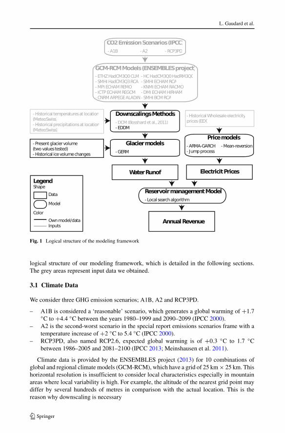
We attempt to simulate future hydropower revenue which is determined by runoff, whole-sale electricity prices, and supply schedules (Gaudard et al. 2013a). Figure 1 highlights the

L. Gaudard et al.

Fig. 1 Logical structure of the modeling framework

logical structure of our modeling framework, which is detailed in the following sections.The grey areas represent input data we obtained.

3.1 Climate Data

We consider three GHG emission scenarios; A1B, A2 and RCP3PD.

– A1B is considered a ‘reasonable’ scenario, which generates a global warming of +1.7C to +4.4 C between the years 1980–1999 and 2090–2099 (IPCC 2000).

– A2 is the second-worst scenario in the special report emissions scenarios frame with atemperature increase of +2 C to 5.4 C (IPCC 2000).

– RCP3PD, also named RCP2.6, expected global warming is of +0.3 C to 1.7 Cbetween 1986–2005 and 2081–2100 (IPCC 2013; Meinshausen et al. 2011).

Climate data is provided by the ENSEMBLES project (2013) for 10 combinations ofglobal and regional climate models (GCM-RCM), which have a grid of 25 km× 25 km. Thishorizontal resolution is insufficient to consider local characteristics especially in mountainareas where local variability is high. For example, the altitude of the nearest grid point maydiffer by several hundreds of metres in comparison with the actual location. This is thereason why downscaling is necessary

Long-term Uncertainty of Hydropower Revenue

Adapting GCM-RCM data to local situations has been performed by twomethods, i.e. theDelta Change Method (DCM) (Bosshard et al. 2011) and the Empirical Distribution DeltaMethod (EDDM) (Gaudard et al. 2013a). For the whole panel of GHG emission scenarios(A1B, A2 and RCP3PD), we used the data provided by C2SM (CH2011, C2SM (2014)).This team applied the DCM (Bosshard et al. 2011). This consists of moving the mean tem-perature and precipitation in historical data to reflect climate forecasting. C2SM simulatesthe meteorological variability by running a random function. It therefore obtains a set of 10time series for each GCM-RCM, i.e. 100 by GHG emission scenarios.

For the scenario A1B, we also applied EDDM (Gaudard et al. 2013a). It differs from theprevious one, because it takes into account the variation in distribution, not only the meanvariation. The impact of climate change on interannual variability is therefore considered.In contrast to DCM, EDDM provides only one path per GCM-RCM. This is due to the factthat the variability is not generated by a stochastic variable like with DCM.

3.2 Glacio-Hydrological Model

High-mountain catchment areas generally have a long-lasting snow cover and a considerabledegree of glacier coverage. This influences the runoff regime and needs to be taken intoaccount in the runoff modeling. For this reason the combined glacio-hydrological modelGERM (Farinotti et al. 2012; Huss et al. 2008) is employed to assess the impact of climatechange on the evolution of runoff. The model considers the processes of accumulation andthe melt of snow and ice masses as well as the glacier evolution. Ablation is basicallya function of air temperature and potential solar radiation. Accumulation is modeled byusing precipitation lapse rates and air temperature to distinguish between liquid and solidprecipitation. Snow redistribution processes (wind, avalanches) are also included. In the laststep, the model evaluates the local water balance given by liquid precipitation, melt waterand evaporation and routes the water through a couple of linear reservoirs in order to mimicthe retention of the water in the catchment area.

The model is forced by daily temperature and precipitation time series from the 1980–2100 time period. Past meteorological data is taken from MeteoSwiss (2013) weatherstations in the vicinity of the catchment area. For future time series the downscaled climatescenarios are used (see Section 3.1). The empirical character of the glacier and runoff modelrequires calibration of various model parameters which is done by means of past ice volumechanges, direct mass balance measurements and runoff records. Gabbi et al. (2012) describethe application of the GERM model to our case study. It provides further details about cal-ibration and validation. If it presents the A1B GHG scenario results, the A2 and RCP3PDones are unpublished so far.

For glacier projections the distribution of ice mass in the modeling domain has to beknown. Due to scarce or non existent measurements of ice-thickness, estimation approachesare commonly used (Farinotti et al. 2009). Our own previous estimations showed a total icevolume of 4.41± 1.02 km3. However, recently performed area-wide ice-thickness measure-ments revealed a smaller ice volume of 3.69± 0.31 km3 (-16 %). We test both initial icevolumes to quantify the sensitivity of our results to this parameter.

3.3 Wholesale Electricity Price Models

For electricity price, we consider one reference, called Ref, which is the repetition of his-torical prices, and three price models, explained below. They are parameterized with EEXGerman electricity spot prices (EEX 2013). This index is more relevant for the long-term

L. Gaudard et al.

forecasting, since it is the expression of the leading exchange market in Europe. The periodof calibration of all our models is 01-Apr-2001 to 31-Mar-2012. In order to get the realprice, we use the Harmonised Index of Consumer Prices (HICP) for Germany provided byEurostat (2013). Thus all our revenues are year 2005 e equivalent.

We consider an explanatory scenario based on past data (EEA 2000; Kowalski et al.2009). Our models do not aimed at forecasting electricity prices, which is almost impossiblein the long-term. We instead adopt a statistical approach and consider various price models.We instead focus on the comparison of uncertainty created by runoff with electricity prices,rather than price forecasting. Based on our underlying aim, our method provides relevantoutcomes.

3.3.1 Common Components to All Models

We provide a detailed explanation of the price models. We thoroughly describe thiscomponent since it is not described in our previous papers. This component is new.

We consider the logarithm of the prices in order to keep the variance more stable (Tsay2010; Wooldridge 2009). The model is therefore as follows:

log(Pt ) = Xst +

23∑

i=1

αiDhoursi,t + α24D

we24,t + εt (1)

where Pt is the hourly electricity spot price [e MWh−1], Xst is the seasonal factor, D

hoursi,t

and Dwe24,t are dummy variables that control hourly variation and gaps between weekday and

weekends. Short term volatility is denoted as εt .The volatility is approached with an ARMA(1,1)-GARCH(1,1) model (Bollerslev 1986;

Box and Pierce 1970). (2) represents the ARMA(1,1) process while (3) to (4) are theGARCH(1,1) processses. The model is commonly used to forecast short-term electricityprices because it is well suited for market with high volatility (Garcia et al. 2005). Wechoose an order (1,1,1,1), which means that the error and its variability are determined byerror at time t − 1.

εt = βmodtot

1 + βmodtot

2 εt−1 + βmodtot

3 δt−1 + δt (2)

δt = σ zt where zt ∼ N (0, 1) (3)

σ 2t = β

modtot

4 + βmodtot

5 σ 2t−1 + β

modtot

6 δ2t−1 (4)

where the set of models is modtot ∈ MRy,MRs ,MRJD and δt is the remaining volatilityof the ARMA(1,1) model. At time t, it is normally distributed and simulated with a standardnormal random variable, zt , and a standard deviation, σt . The latter varies and follows aGARCH(1,1) process.

3.3.2 The Three Electricity Price Models

The difference between the electricity price models lies in the way they treat the seasonalfactor, Xs

t , in (1). By taking into consideration various price models, it can identify the

Long-term Uncertainty of Hydropower Revenue

uncertainty of future prices, in particular linked to seasonality. We also assess whetherinterannual and intra-annual variability is important for future revenues. Below we brieflydescribe the models and provide some relevant references.

We consider two mean-reversing models, called MRy and MRs (Uhlenbeck and Orn-stein 1930). These processes are commonly used in raw commodity investment analysesbecause under certain hypotheses prices are attracted by production costs. They are definedas follows:

Xmodt = κmod(μmod − X

yt )t + ηmodWt (5)

Wt = zt

√t (6)

where the set of models is mod ∈ MRy,MRs, κ is the reversion speed and μ the long-term mean. η is the Brownian motion term, which explains why Wt follows the Wienerprocess represented in (6). As in (3), zt is a standard normal random variable.

MRy is realitively stable. Its mean yearly price may change, but the intra-annual profiledo not change, as in:

Xst = γ

MRy

0 + XMRy

t +3∑

j=1

γMRy

j Dseasonj,t (7)

where XMRy

t is an annual mean [e MWh−1] that follows a mean reversion process.MRs considers that the mean price of each season, X

MRst , follows a mean reversion

process. In contrast to MRy , the season with the mean highest prices may change from thehistorical pattern. This price model is then formulated as:

Xst = γ

MRs

0 + XMRst (8)

where XMRst is a seasonal mean [e MWh−1], i.e. average over three months, that follows a

mean reversion process.The mean-reversing jump diffusion model, called MRJD, allows to consider that price is

attracted by production cost, like the two previous ones (Kaminski 1997). However, someshocks may perturb the price. One may observe a jump over a certain period of time, whichmay be formalized as:

Xst = γMRJD

0 +3∑

j=1

γMRJDj Dseason

j,t + XMRJDt (9)

XMRJDt = κMRJD(μMRJD − X

yt )t + ηMRJDWt︸ ︷︷ ︸

mean-reversion process

+ Jqt︸ ︷︷ ︸jump

where J ∼ N (ν, θ) (10)

qt = 1 with probability λt

0 with probability (1 − λ)t(11)

where XMRJDt is the daily mean price [eMWh−1] and qt is a poisson process that produces

infrequent jump of size J .

L. Gaudard et al.

3.4 Hydropower Plant Management

The operator of the hydropower installation aims to maximize profit. Because the vari-able costs are small for this technology, they can be ignored in this analysis. The objectivefunction is given by Forsund (2007):

OF(b) = g ρ η f t

(t=T∑

t=1

ht bt Pt

)+ RT (12)

where g is the acceleration due to gravity [m s−2], ρ the water density [kg m−3], η the plantefficiency, f the water flow through the turbine [m3 s−1], ht the hydraulic head [m], Pt theelectricity spot price [e Wh−1]. The objective function is defined on the time horizon T

and for a binary variable bt which indicates whether one produces or not.The optimization problem and its constraints are formalized as:

maxb

OF(b) (13)

Vt = Vt−1 + It t − f bt t (14)

ht = (Vt ) (15)

Vmin < Vt < Vmax (16)

bt ∈ 0, 1 (17)

where Vt is the reservoir content at time t [m3], It the water intake [m3 s−1], ht is a functionof Vt , and Vmin, Vmax are the capacity limits of the reservoir.

We optimize over a time horizon of two years and validate the first one. Then, we movethe windows for the following optimization one year later. To tackle the residual watervolume, RT , we fix the final volume after two years at the initial level.

The objective function is maximized with a local search method, called ThresholdAccepting (Dueck and Scheuer 1990; Moscato and Fontanari 1990). The algorithm startswith a random turbine schedule, it evaluates the corresponding objective function value.Then it considers a solution in the neighborhood by introducing a small random perturba-tion to the current schedule and evaluates the new corresponding objective function value.The new solution is accepted if it is no worse than a given threshold. This means that thealgorithm also allows down steps in order to escape local minima. Of course, the thresholddecreases gradually to zero which means that in the final steps only solutions which improvethe objective functions are accepted. A data driven procedure determines the thresholdsequence as described by Winker and Fang (1997) and adapted by Gilli et al. (2006). Thisalgorithm as a whole has proven its effectiveness to find an acceptable optimum. We dohowever acknowledge that other algorithms also exist as reviewed by Ahmad et al. (2014).For instance, some papers consider a genetic algorithm (Hincal et al. 2011; Cheng et al.2008) or a simulated annealing one (Teegavarapu and Simonovic 2002). Some papers alsoinvestigate multi-objective optimization rather than one objective function (Liao et al. 2014;Kougias et al. 2012).

We assume a clear-sighted manager, i.e. he knows in advance the price and runoff. Evenif this hypothesis is optimistic (Tanaka et al. 2006), it is commonly used in papers for com-putational efficiency (Francois et al. 2015; Maran et al. 2014; Hendrickx and Sauquet 2013;Schaefli et al. 2007). Since we look at trends and do not aim to forecasting exact futurerevenue, this hypothesis does not affect our conclusions.

Long-term Uncertainty of Hydropower Revenue

We validated our model by using historical data. Once the optimization performed withpast runoff and electricity prices, we have compared the hourly, weekly and seasonal pro-duction with the actual production. We also verified that the lake level followed the samepattern in our simulation as in the real life. Gaudard et al. (2013a) provides more detailsabout the management model.

3.5 Field Site

The case study is based on the hydropower plant of Mauvoisin, situated in the Swiss Alps(7o35′E, 4600′N). A reservoir gathers the runoff coming from nine glaciers (Petit Com-bin, Corbassiere, Tsessette, Mont Durand, Fenetre, Crete Seche, Otemma, Brenay, Gietro),which covered in 2009 40 % of the catchment area (Gabbi et al. 2012).

The reservoir volume is 192 × 106 m3, which represents 624GWh. The mean multi-yearproduction is 1040GWh (years 1999–2009), 53 % in winter and 47 % in summer (FMM2009). The reservoirs in the Alps transfer energy from summer, when snow and glaciersmelt, to winter, when electricity demand is high.

Several studies were carried out on the impact of climate change in the Bagne Valleywhere the Mauvoisin power plant is situated (Gaudard 2015; Gaudard et al. 2013a; Gabbiet al. 2012; Terrier et al. 2011; Schaefli et al. 2007). So far, the operators have taken advan-tage of the glacier melting, which increases the annual volume of water. According to Gabbiet al. (2012), this trend will persist for the next 20 years. The annual runoff will subsequentlydecrease in the second half of the century. By 2100, glaciers are expected to disappear in thiscatchment area. Thanks to the reservoir, the power plant operator may, however, mitigate theeffects resulting from the runoff seasonality (Gaudard et al. 2013a). A new pumped-storagemay even be built from 2040 on the surface released by the glacier and therefore increasesenergy production on the site (Gaudard 2015; Terrier et al. 2011)

4 Results

In this section, we show how the scenarios and models affect the key variables of our study,i.e. climate, runoff, prices and revenue. The uncertainty analysis follows.

4.1 Climate Data

The evolution of air temperature and precipitation depends on the GHG emission scenario.The warmest scenario, i.e. A2, expects a mean local air temperature of +2 C for the period2091–2100 (data corresponds to an altitude of 2921 m a.s.l.). It is 3.7 C warmer than thehistorical records for the period 2000-2009. Scenario A1B provides a medium situation. Themean local air temperature is +1.4 C for 2091–2100. The coolest scenario, i.e. RCP3PD,stabilizes the mean yearly temperature at −0.7 C which is below the melting point. Albeitthose three GHG emission scenarios cover a large range of future evolutions, none affectsthe mean precipitation over the century. It stays at 3.7 mm day−1.

In this study, we consider 10 GCM-RCM with 10 paths for each. The gaps between theextreme GCM-RCM may be significant. In the case of the A1B scenario and consideringthe end of the century, the gap is about 2 C for air temperature and 0.4 mm day−1 forprecipitation. Whilst the coolest GCM-RCM predicts a mean temperature close to 0 C, thewarmest reaches 2 C. It shows that the variability between the GCM-RCM is not far fromthe variability between GHG emission scenarios. Research investigations can fortunately

L. Gaudard et al.

reduce this epistemic uncertainty by using data from a large set of GCM-RCM, as done inour study.

The downscaling method, i.e. EDDM and DCM, affects the outcome. The expectedmean temperature does not significantly differ between the two methods unlike the interan-nual temperature variability. The latter remains stable with DCM while the EDDM methodslightly influences it. Beside temperatures, DCM does not affect the mean precipitation andits interannual equivalent, while the EDDM affects both. The mean precipitation increasesby 0.1 mm day−1, while the interannual variability rises. This downscaling step representsa source of epistemic uncertainty currently tackled by climatologists.

4.2 Glacier Evolution and Runoff

Figure 2 represents the evolution of inflows in the Mauvoisin reservoir for the three GHGemission scenarios. All emission scenarios have the same general pattern. The runoffincreases slightly until 2040 compared to present-day conditions. Afterwards, inflowsdecrease by a similar value. While the mean recorded runoff was of 292 × 106 m3 for1981–2010, it becomes for the period 2021–2050 of 302, 300 and 297 × 106 m3 for A1B,A2 and RCP3PD, respectively. For the period 2071–2100, the computed runoff is 243,245 and 242 × 106 m3. While the GHG emission scenario largely affect the warming, itunexpectedly represents a low source of uncertainty in terms of runoff.

The 10 GCM-RCM do not predict the same pattern. The mean runoff for 2071–2100goes from 224 × 106 m3 to 260 × 106 m3. The percentage error is about 8 %. It shows thatstudies based on few GCM-RCM suffer of high epistemic uncertainty.

The downscaling method (shown in the upper left-hand panel) has a higher impact byaffecting the mean runoff. The EDDM forecasts a mean runoff of 262 × 106 m3 for 2071–2100. This is 19 × 106 m3 higher than the mean runoff obtained with the DCM. This isalso beyond the extreme GCM-RCM outcomes.

100

200

300

400A1B

100

200

300

400A2

1980 2000 2020 2040 2060 2080 2100100

200

300

400

Ann

ual r

unof

f [10

m

3 ]

year

RCP3PD

1980 2000 2020 2040 2060 2080 2100100

200

300

400

year

A1B, overestimated ice

historicalforecasting pathmean forecastingEDDM forecasting

6

Fig. 2 Historical (1980–2009) and forecasted runoff (2009–2100) into the Mauvoisin reservoir for each ofthe GHG emission scenarios and the situation with overestimated initial ice volume (bottom right panel)

Long-term Uncertainty of Hydropower Revenue

The projected interannual variability is not affected by the DCM. It varies around thehistorical one between 26 and 31 × 106 m3. But it rises to 36 × 106 m3 with EDDM. Asargued by Quintana Segui et al. (2010), the downscaling method brings epistemic uncer-tainty and could be further improved The sensitivity of our results to the initial ice volumeis relatively low. The bottom right graph of Fig. 2 shows the influence of overestimating thisvariable for the runoff considering the A1B GHG emission scenario. The runoff increasesby about 10 % in a first phase and then it decreases to attain a mean annual runoff of241 × 106 m3 y−1 in the last decades of the 21st century. It is surprisingly lower, but withinthe error term, than with the correct ice volume. Moreover, Gabbi et al. (2012) have alreadyhighlighted that the shape of the glacier, not only the volume, has a major influence on theresults.

4.3 Electricity Prices

Table 2, in Annex, shows that the parameters of the price models are highly significant. Thevalidation of each models is based on a comparison between the simulated prices and thehistorical ones. We have checked that the daily, weekly, and if applicable seasonal variationsreflect the price behavior in the Continental Central-South area of Europe.

The volatility partially affects the annual mean prices and its interannual variability. Theyare 41 (9.7), 46 (6.1), and 40 (2.0) eMWh−1 in the case of MRy , MRs , and MRJD respec-tively (interannual variability in brackets). These values remain stable over the 120-yearperiod, thanks to the mean reversion process. They therefore remain close to the historicalmean price, which was about 39 (10.3) eMWh−1, while the interannual volatility is under-estimated. It underlines the difficulty of finding models that are representative yet maintaina level of variability.

Our models investigate the impact of seasonality only. We also tested a geometric Brow-nian motion model, which is not presented in this paper. The price was highly volatilesince no reverting process was considered. The quantitative results led to one main obviousconclusion; if the annual price can evolve, the variability of the price overtakes all otheruncertainties. The interannual variability of the revenue became larger than the expectedrevenue.

4.4 Revenue

The annual revenue represents a merging outcome enabling comparison between theimpacts of every input. Table 1 presents it in terms of a mean and a standard deviation.We show the results for each electricity price scenario for the A1B GHG emission, other-wise we only refer to the historical price, i.e. Ref price model. This table also includes theimpact of the downscaling method and initial ice volume. Trends from the various scenar-ios or models must be compared, rather than the numbers being reviewed in isolation. Asalready stated, we are not aiming to forecast future revenue here, we are in fact investigatinguncertainty.

Our results show that climate change affects mean annual revenue, although the varia-tion between various GHG emission scenarios is low (lines 1, 6 and 7). This is particularlystriking for the period 2071–2100. During this period, the runoff resulting from the melt-ing glacier will be low because of glacier exhaustion (A1B and A2) or air temperature

L. Gaudard et al.

Table 1 Mean and standard deviation (in brackets) of annual revenue in 106 e for various RCM-GCM,downscaling methods and initial ice volume

Climate Electricity price 1981–2010 2021–2050 2071–2100

1 A1B Ref 80.5 86.5 70.0

(31.5) (32.5) (27.5)

2 A1B MRy 86.5 90.5 75.0

(35.5) (35.5) (30.0)

3 A1B MRs 95.5 100.0 84.0

(25.0) (24.5) (22.5)

4 A1B MRJD 89.5 92.5 79.5

(14.0) (14.0) (13.5)

6 A2 Ref 80.5 81.0 69.0

(31.5) (32.0) (27.0)

7 RCP3PD Ref 80.5 80.5 68.0

(31.5) (32.0) (26.0)

8 A1B, EDDM Ref 80.5 84.5 75.0

(31.5) (32.5) (29.5)

9 A1B, old ice volume Ref 80.5 87.0 72.0

(31.5) (32.5) (28.5)

stabilization (RCP3PD). The uncertainty is not necessarily shown to lie in the GHGemission scenarios.

It is interesting to note that annual revenue is not linearly related to the annual runoff.In the medium term, the A2 and RCP3PD GHG emission scenarios do not (negatively)affect revenue as we notice a runoff rise. In contrast, the A1B scenario computed revenueis surprisingly high whereas the annual runoff was close to the two other GHG emissionscenarios. The seasonality can explain this result, even if the reservoir partially addressesthis.

The difference between the 10 considered GCM-RCM ranges from 63 to 73.5× 106 e for the A1B GHG emission scenario and the period 2071–2100 (not given in thetable). This gap is higher than the difference between GHG emission scenarios. Therefore,studies based on few climate models carry a high degree of epistemic uncertainty.

The uncertainty brought by the initial ice volume is not as high as the uncertainty result-ing from the downscaling method (comparison line 1, 8 and 9). The computed mean revenuewith the EDDM downscaling method is higher than the most extreme GCM-RCM computedwith the DCM method. EDDM also tends to smooth the revenue evolution. It increases lessin the medium term and decreases less in the second half of the century. Due to a lack ofdata, we were not able to assess more downscaling methods, however this would have beenbeneficial. This is an ongoing research in climatology (Fowler et al. 2007). The initial icevolume surprisingly has a relatively small impact.

The electricity price models comparison can barely demonstrate trends (lines 1 to 4).Our models are conservative as they do not consider drift. However, even through this

Long-term Uncertainty of Hydropower Revenue

hypothesis, the mean revenue widely differs from model to model. For the initial period1981–2010, the mean revenue is not linearly correlated to the mean price. For instance,Ref and MRJD models have a close mean price, but the revenues differ significantly. Ifthe mean annual revenue matters, the seasonality and the volatility of the price do too. Thetrouble is that if the mean price has proven to be hard to predict, the volatility is even morepronounced.

This issue is particularly important as we can demonstrate that revenue is mainly cor-related to price. For 2071–2100, the revenue gap between annual revenue is higher whenconsidering various price models rather than various GHG emission scenarios. In fact, thecorrelation coefficient between mean runoff and revenue is 0.16, while it is 0.91 for meanannual price and revenue. Therefore, price is the key factor for determining future revenue,however it is also the least predictable factor.

4.5 The Three Dimensions of Uncertainty

We discuss the main uncertainties detailed in our research, in particular those uncertain-ties that are most relevant to policy makers. In this regard, we cover the various elementsidentified byWalker et al. (2003). Based on the above results, the level of uncertainty is clas-sified as statistical, scenarios and ignorance. We also distinguish the nature, i.e. epistemicor variability.

Context:Level: Climate and energy policy should factor in the high degree of uncertainty. Because

it is impossible to predict the GHG emissions and the electricity prices in the long-term,scenarios should be used. Concerning electricity prices, a level of ignorance should berecognized because market architecture and market structure are still evolving.

Nature: In the medium term, these uncertainties have an epistemic nature because theycould be reduced by improving models. In the long-term, they should be characterizedas ‘variability uncertainty’ because the randomness of nature, human behavior, socio-economic and technological dynamics prevail. Over such a period, the is not a model thatappears more relavent than another and our approach, i.e. to compare various models andscenarios, appears the most appropriate.

Model:Level: The level of uncertainty linked to the model is for the most part statistical.Nature: One should expect improvements in modeling as significant public and private

funding is now available. Uncertainty is therefore of an epistemic nature, although it remainsrelatively low compared to the variability provoked by runoff, future prices, market design,etc. (see ‘context’ above and ‘inputs’ below).

Inputs:Level: Uncertainty relating to runoff and electricity price scenarios turns out to be closely

linked to ‘context’. Here, we discuss the scenarios as opposed to the outcomes themselves.The nature and level therefore corresponds to climate and energy policy. Concerning data,the electricity price time series shows a statistical level of uncertainty.

Nature: Regarding the nature, one should point out an epistemic uncertainty in the assess-ment of the initial ice volume and in the downscaling methods (DCM and EDDM). Wetherefore provide a sensitivity analysis with respect to these inputs. However, most datashows ‘variability uncertainty’.

L. Gaudard et al.

Parameters:Level: The parameters are determined by statistical methods (calibration techniques

included).Nature: They are tainted by epistemic uncertainty as far as estimations can be perfected.

Given the fact that longer time series will be available in time, estimators will, as a result,improve.

Outcomes:Level: The level of uncertainty of the intermediate and final outcomes, i.e. runoffs,

electricity prices and revenue, are essentially ‘scenario’. The GHG emission and elec-tricity price scenarios directly influence the outcomes. However Mauvoisin’s long-term runoff uncertainty becomes mostly statistical due to the minimal gap between GHGscenarios.

Nature: The nature of the runoff uncertainty evolves with time. In our research, weconsider a large panel of GCM-RCM therefore limiting the resulting uncertainty. Themain cause of uncertainty is therefore determined by other sources. In the medium term,uncertainty is primarily brought by the three GHG emission scenarios which depend onsocio-economic variables. Those variables are barely predictable thus leading to a dominantvariability uncertainty. In the long run, the situation switches. The downscaling method sig-nificantly impacts the mean runoff for the period 2071–2100. It overtakes the gap betweenthe three GHG emission scenarios, which end up with a similar mean runoff. Climatologistsare currently improving the downscaling method. We can therefore state that the long-rununcertainty is mostly epistemic.

The nature of electricity price uncertainty follows the reverse trend. In the medium-term,the epistemic uncertainty is high. Scientists constantly build better models to forecast elec-tricity prices. They also adapt the forecasting in light of new information. The uncertainty upto 2021–2050 will remain mostly epistemic. In the long-run, the nature uncertainty becomes‘variability’, because it is impossible to forecast precise prices over such a long timeframeregardless of the model’s quality. The unpredictable behavior component becomes funda-mental. As already mentioned, the use of different models and sensitivity analyses seems tobe the most appropriate approach.

The uncertainty of revenue is directly induced by future runoff and electricity priceuncertainty. Following the discussion of the two former paragraphs, the nature of revenueuncertainty is established as both epistemic and variability.

5 Discussion

We should point out that information about uncertainty is of great value to decision-makers.Improving the models reduces the epistemic uncertainty, whereas business and regulatorystrategies can address variability. The dimension ‘nature’ shows who should deal with theuncertainty, i.e. scientists or decision-makers.

The ‘level’ may help in identifying the tools that should be considered to managethe uncertainty. In economics, the statistical uncertainty is tackled by risk managementmethods, e.g. value at risk. The scenario level is close to the knightian definition of uncer-tainty, i.e. probability cannot be estimated. Many rational decision making methods addressthese kinds of issues, e.g. minimum regret criteria. Finally, the ignorance cannot really be

Long-term Uncertainty of Hydropower Revenue

managed in any way. We cannot assume to know the unknown. However the context of thestudy must be clearly defined in order to limit the impact of ignorance on the results as faras possible.

This paper discusses the epistemic uncertainty occurring at various levels of the model.However specific literature on the diverse components is wide. The uncertainty relat-ing to the climate modelis discussed at global and regional level by Deque et al. (2007)and Murphy et al. (2004). The various Intergovernmental Panel on Climate Changereports also provide valuable discussion on this issue (IPCC 2015). Monier et al. (2015)present a new framework to assess climate uncertainty which is close to ours. Theirresults show that the largest uncertainty in terms of temperature comes from climatepolicy. Gabbi et al. (2014) test five different glacier melt models and show that thechoice of the melt approach is crucial. Finally, Teng et al. (2012) analyse a case studywhere uncertainty is mostly led by GCM rather than the rainfall model. These studies,together with our results, show that uncertainty, like forecasting, is case study and modelrelated.

As pointed out all throughout this paper, price uncertainty is far more critical than runoffuncertainty. Linderoth (2002) tests various energy consumption forecasts performed by theInternation Energy Agency. He shows that forecast errors are significant. Given that priceis even less predictable than consumption, we can conclude that the problem is even wider.By arguing that scenario analysis and mixed method are valuable in short-term managementtoo, O’Mahony (2014) supports our approach and conclusion. Therefore, uncertainty relatedto energy price quickly shifts from epistemic uncertainty to variability.

If decision makers must account for the epistemic uncertainty, they essentially mustmanage variability. First, they can act on the ‘level’. One way is to develop market designand risk-hedging tools. Future markets already exist but should be enhanced. However themost important is that energy policy can reduce uncertainty at the ignorance level. Severalenergy utilities at present are facing forms of turmoil that were only partially predictable.The phase-out of nuclear power in some countries or the large subsidies to the renew-ables are worth mentioning. The alternative way to deal with variability is by increasingflexibility. However, the regulatory framework can represent an obstacle from this pointof view. For instance, the water rights in some countries limit the plant operator’s flexi-bility. The legal framework often makes it difficult to adopt a real option approach. Forinstance, some hydropower operators must re-negotiate their water right if they want toupdate the design of their installation. This constraint makes it difficult to manage highuncertainty.

6 Conclusions

Decision-makers cannot avoid uncertainty. Several studies focus on projections, but anassessment of the uncertainties is seldom carried out. Our model integrates runoff andelectricity prices in a common framework in order to evaluate revenue. Based on those quan-titative results, we carry out an uncertainty analysis, which is a critical issue for the futureof hydropower.

Specific tools must be developed in order to tackle uncertainty. Hydropower is a capital-intensive technology with a long lifetime. Forecasting revenue over the entire life of the

L. Gaudard et al.

project is impossible. The limits of previsions should be acknowledged and some methodsmust be developed accordingly. Assessing uncertainty is only the first step in a strategy toensure the best possible future for hydropower.

7 Annex

Table 2 Values of the electricity price parameters

MRy MRs MRJD

Cst γ0 −0.050 −0.093 3.487

(0.007) (0.006) (0.008)

ARMA β1 0.009 0.010 -0.008

(3e-4) (3e-4) (3e-4)

β2 0.828 0.791 0.617

(9e-4) (9e-4) (0.002)

β3 0.241 0.252 0.314

(0.002) (0.002) (0.002)

GARCH β4 0.007 0.007 0.004

(3e-5) (3e-5) (2e-5)

β5 0.434 0.405 0.545

(0.001) (0.001) (0.001)

β6 0.505 0.535 0.455

(0.002) (0.002) (0.002)

Mean-reversing μ 3.620 3.592 1.061

(0.096) (0.210) (0.005)

η 0.338 0.421 0.199

(0.060) (0.024) (8e-4)

κ 0.909 1.016 0.166

(0.151) (0.359) (8e-4)

Jump diffusion ν 0.196

(0.002)

θ 0.839

(0.009)

λ 0.047

(0.001)

Seasonal dummies γ1,2,3 Yes No Yes

Long-term Uncertainty of Hydropower Revenue

Acknowledgments This study was carried out within the framework of the Swiss research programme61(www.nfp61.ch). We are grateful to prof. Martin Funk and prof. Manfred Gilli for providing valuablescientific inputs and proofreading the paper. We also thank Force Motrices de Mauvoisin for sharing theirexpertise.

Compliance with Ethical Standards

Conflict of interests The authors declare that they have no conflict of interest.

Open Access This article is distributed under the terms of the Creative Commons Attribution 4.0 Inter-national License (http://creativecommons.org/licenses/by/4.0/), which permits unrestricted use, distribution,and reproduction in any medium, provided you give appropriate credit to the original author(s) and the source,provide a link to the Creative Commons license, and indicate if changes were made.

References

Ahmad A, El-Shafie A, Razali S, Mohamad Z (2014) Reservoir Optimization in Water Resources: a Review.Water Resour Manag 28:3391–3405. doi:10.1007/s11269-014-0700-5

Bollerslev T (1986) Generalized autoregressive conditional heteroskedasticity. J Econ 31:307–327.doi:10.1016/0304-4076(86)90063-1

Bosshard T, Kotlarski S, Ewen T, Schar C (2011) Spectral representation of the annual cycle in the climatechange signal. Hydrol Earth Syst Sci 15:2777–2788

Box G, Pierce D (1970) Distribution of residual autocorrelations in autoregressive-integrated moving averagetime series models. J Am Stat Assoc 65:1509–1526

C2SM (2014) www.c2sm.ethz.ch (site accessed 06 February 2014). Center for Climate Systems Modeling,ETHZ

Cheng CT, Wang WC, Xu DM, Chau KW (2008) Optimizing hydropower reservoir operation using hybridgenetic algorithm and chaos. Water Resour Manag 22:895–909. doi:10.1007/s11269-007-9200-1

Creswell J, Plano Clark V (2011) Designing and conducting mixed methods research, 2nd. SAGE Publica-tions

Deque M, Rowell DP, Luethi D, Giorgi F, Christensen JH, Rockel B, Jacob D, Kjellstrom E, De CastroM, Van den Hurk B (2007) An intercomparison of regional climate simulations for Europe: assessinguncertainties in model projections. Clim Chang 81:53–70. doi:10.1007/s10584-006-9228-x

Dueck G, Scheuer T (1990) Threshold accepting. A general purpose optimization algorithm superior tosimulated annealing. J Comput Phys 90:161–175

EEA (2000) Cloudy crystal balls - an assessment of recent European and global scenario studies and mod-els www.eea.europa.eu/publications/Environmental issues series 17 (site accessed 05 January 2015).European Environment Agency

EEX (2013) www.eex.com (site accessed 04 August 2013). European Energy ExchangeENSEMBLES project (2013) www.ensembles-eu.org (site accessed 01 October 2013)Eurostat (2013) ec.europa.eu/eurostat (site accessed 31 August 2013)Farinotti D, Huss M, Bauder A, Funk M, Truffer M (2009) A method to estimate the ice volume and ice-

thickness distribution of alpine glaciers. J Glaciol 55:422–430Farinotti D, Usselmann S, Huss M, Bauder A, FunkM (2012) Runoff evolution in the Swiss Alps: Projections

for selected high-Alpine catchments based on ENSEMBLES scenarios. Hydrol Processes 26:1909–1924Finger D, Vis M, Huss M, Seibert J (2015) The value of multiple data set calibration versus model complex-

ity for improving the performance of hydrological models in mountain catchments. Water Resour Res51:1939–1958. doi:10.1002/2014WR015712

FMM (2009) Management reports. Forces motrices de MauvoisinForsund F (2007) Hydropower Economics. In: International Series in Operations Research and Management

Science. SpringerFowler HJ, Blenkinsop S, Tebaldi C (2007) Linking climate change modelling to impacts studies:

recent advances in downscaling techniques for hydrological modelling. Int J Climatol 27:1547–1578.doi:10.1002/joc.1556

L. Gaudard et al.

Francois B, Hingray B, Creutin JD, Hendrickx F (2015) Estimating water system performance under cli-mate change: influence of the management strategy modeling. Water Resour Manag 29:4903–4918.doi:10.1007/s11269-015-1097-5

Gabbi J, Carenzo M, Pellicciotti F, Bauder A, Funk M (2014) A comparison of empirical and physicallybased glacier surface melt models for long-term simulations of glacier response. J Glaciol 60:1140–1154

Gabbi J, Farinotti D, Bauder A, Maurer H (2012) Ice volume distribution and implications on runoffprojections in a glacierized catchment. Hydrol Earth Syst Sci 16:4543–4556

Garcia R, Contreras J, Van Akkeren M, Garcia J (2005) A GARCH forecasting model to predict day-aheadelectricity prices. IEEE Trans Power Syst 20:867–874. doi:10.1109/TWRS.2005.846044

Gaudard L (2015) Pumped-storage project: A short to long term investment analysis including climatechange. Renew Sust Energy Rev 49:91–99. doi:10.1016/j.rser.2015.04.052

Gaudard L, Gilli M, Romerio F (2013a) Climate change impacts on hydropower management. Water ResourManag 27:5143–5156

Gaudard L, Romerio F (2014) The future of hydropower in Europe: Interconnecting climate, markets andpolicies. Environ Sci Policy 37:172–181

Gilli M, Kellezi M, Hysi H (2006) A data-driven optimization heuristic for downside risk minimization. JRisk 8(3):1–18

Hamududu B, Killingtveit A (2012) Assessing climate change impacts on global hydropower. Energies5:305–322

Hendrickx F, Sauquet E (2013) Impact of warming climate on water management for the Ariege River basin(France). Hydrol Sci J 58:976–993. doi:10.1080/02626667.2013.788790

Hill Clarvis M, Fatichi S, Allan A, Fuhrer J, Stoffel M, Romerio F, Gaudard L, Burlando P,Beniston M, Xoplaki E, Toreti A (2014) Governing and managing water resources under chang-ing hydro-climatic contexts: The case of the Upper-Rhone basin. Environ Sci Policy 43:56–67.doi:10.1016/j.envsci.2013.11.005

Hincal O, Altan-Sakarya AB, Ger AM (2011) Optimization of multireservoir systems by genetic algorithm.Water Resour Manag 25:1465–1487. doi:10.1007/s11269-010-9755-0

Huss M, Farinotti D, Bauder A, Funk M (2008) Modelling runoff from highly glacierized Alpine drainagebasins in a changing climate. Hydrol Process 22:3888–3902

IEA (2005) Variability of wind power and other renewables: Management options and strategies. Interna-tional Energy Agency, Paris

IPCC (2000) Special report on emissions scenarios. www.ipcc.ch (site accessed 14 January 2014). Intergov-ernmental Panel on Climate Change, Geneva

IPCC (2013) Climate Change 2013: The Physical Science Basis. Contribution of Working Group I to theFifth Assessment Report of the Intergovern- mental Panel on Climate Change. In: Stocker TF, Qin D,Plattner G-K, Tignor M, Allen SK, Boschung J, Nauels A, Xia Y, Bex V, Midgley PM (eds). CambridgeUniversity Press, NY, USA. Intergovernmental Panel on Climate Change, Geneva

IPCC (2015) www.ipcc.ch (site accessed 15 November 2015)Kaminski V (1997) The challenge of pricing and risk managing electricity derivatives. In: The US Power

Market. Risk Books, London, pp 149–171Kougias I, Katsifarakis L, Theodossiou N (2012) Medley multiobjective harmony search algorithm:

Application on a water resources management problem. Eur Water 39:41–52Kowalski K, Stagl S, Madlener R, Omann I (2009) Sustainable energy futures: Methodological chal-

lenges in combining scenarios and participatory multi-criteria analysis. European Journal of Oper-ational Research 197:1063–1074. doi:10.1016/j.ejor.2007.12.049. 19th Mini EURO Conference onOperational Research Models and Methods in the Energy Sector, Coimbra, Portugal, Sep 06-08,2006

Liao X, Zhou J, Ouyang S, Zhang R, Zhang Y (2014) Multi-objective artificial bee colony algorithm forlong-term scheduling of hydropower system: A case study of china. Water Util J 7:13–23

Linderoth H (2002) Forecast errors in IEA-countries’ energy consumption. Energy Policy 30:53–61.doi:10.1016/S0301-4215(01)00059-3

Madani K, Lund JR (2010) Estimated impacts of climate warming on california’s high-elevation hydropower.Clim Chang 102:521–538. doi:10.1007/s10584-009-9750-8

Majone B, Villa F, Deidda R, Bellin A (2015) Impact of climate change and water use policies on hydropowerpotential in the south-eastern alpine region. Science of The Total Environment in press. http://www.sciencedirect.com/science/article/pii/S004896971530067X, doi:10.1016/j.scitotenv.2015.05.009

Maran S, Volonterio M, Gaudard L (2014) Climate change impacts on hydropower in an alpine catchment.Environ Sci Policy 43:15–25

Long-term Uncertainty of Hydropower Revenue

Meinshausen M, Smith SJ, Calvin K, Daniel JS, Kainuma MLT, Lamarque JF, Matsumoto K, MontzkaSA, Raper SCB, Riahi K, Thomson A, Velders GJM, Van Vuuren DP (2011) The RCP greenhouse gasconcentrations and their extensions from 1765 to 2300. Clim Chang 109:213–241

MeteoSwiss (2013) www.meteosuisse.ch (site accessed 13 July 2013). Federal Office of Meteorology andClimatology

Monier E, Gao X, Scott JR, Sokolov AP, Schlosser CA (2015) A framework for modeling uncertainty inregional climate change. Clim Chang 131:51–66. doi:10.1007/s10584-014-1112-5

Moscato P, Fontanari J (1990) Stochastic versus deterministic update in simulated annealing. Phys Lett A146:204–208

Murphy J, Sexton D, Barnett D, Jones G, Webb M, Stainforth D (2004) Quantification of mod-elling uncertainties in a large ensemble of climate change simulations. Nature 430:768–772.doi:10.1038/nature02771

O’Mahony T (2014) Integrated scenarios for energy: A methodology for the short term. Futures 55:41–57.doi:10.1016/j.futures.2013.11.002

Quintana Segui P, Ribes A, Martin E, Habets F, Boe J (2010) Comparison of three downscaling methods insimulating the impact of climate change on the hydrology of Mediterranean basins. J Hydrol 383:111–124. doi:10.1016/j.jhydrol.2009.09.050

Schaefli B (2015) Projecting hydropower production under future climates: a guide for decision-makers andmodelers to interpret and design climate change impact assessments. WIREs Water 2:271–289

Schaefli B, Hingray B, Musy A (2007) Climate change and hydropower production in the Swiss Alps: Quan-tification of potential impacts and related modelling uncertainties. Hydrol Earth Syst Sci 11:1191–1205

SHARE project (2013) Handbook: A problem solving approach for sustainable management of hydropowerand river ecosystems in the Alps. www.alpine-space.eu (site accessed 14 January 2014)

Tanaka SK, Zhu T, Lund JR, Howitt RE, Jenkins MW, Pulido MA, Tauber M, Ritzema RS, Ferreira IC(2006) Climate warming and water management adaptation for California. Clim Chang 76:361–387.doi:10.1007/s10584-006-9079-5

Teegavarapu R, Simonovic S (2002) Optimal operation of reservoir systems using simulated annealing. WaterResour Manag 16:401–428. doi:10.1023/A:1021993222371

Teng J, Vaze J, Chiew FHS, Wang B, Perraud JM (2012) Estimating the relative uncertainties sourced fromgcms and hydrological models in modeling climate change impact on runoff. J Hydrometeorol 13:122–139. doi:10.1175/JHM-D-11-058.1

Terrier S, Jordan F, Schleiss A, Haeberli W, Huggel C, Kunzler M (2011) Optimized and adapted hydropowermanagement considering glacier shrinkage scenarios in the Swiss Alps. In: Proceeding of InternationalSymposium on Dams and Reservoirs under Changing Challenges. CRC Press, Taylor & Francis Group,London, pp 497–508

THINK Project (2013) Some thinking on European energy policy: Think tank advising the EuropeanCommission on mid- and long-term energy policy. think.eui.eu (site accessed 13 January 2014)

Tsay S. R (2010) Analysis of Financial Time Series. WileyUhlenbeck G, Ornstein L (1930) On the theory of Brownian motion. Phys Rev 36:823–841Walker W, Harremoes P, Rotmans J, Van Des Sluijs J, Van Asselt M, Janssen P, Krayer Von Krauss M (2003)

Defining uncertainty - a conceptual basis for uncertainty management in model-based decision support.Integr Assess 4:5–17

Winker P, Fang K (1997) Application of threshold-accepting to the evaluation of the discrepancy of a set ofpoints. Siam J Numer Anal 34:2028–2042. doi:10.1137/S0036142995286076

Wooldridge JM (2009) Introductory Econometrics: A Modern Approach, 4th. CENGAGE Learning, Canada