* Copyright by Barnett Sivon & Natter P.C., Attorneys at Law, Washington, DC. Reproduced by permission. Bill Longbrake is Executive-in-Residence at the Robert H. Smith School of Business, University of Maryland.

LONGBRAKE LETTER – November 2017

Bill Longbrake*

I. About As Good As It Gets, But Good Times Could Persist for Several More Months

Depending upon whom you talk to, the next recession could happen as soon as the second half of 2018 or is at least two years or longer in the future. But, for now all seems well and synchronized global forward momentum remains very strong.

As prospects rise for significant tax reform legislation to be enacted and take effect at the beginning of 2018, this stimulus boost is likely to extend the current expansion and push off the timing of the next recession. But, because the stimulus is coming during the mature phase of the cycle when the economy is already at full employment, it raises the risks of overheating and a potentially tighter monetary policy down the road. Amplifying the business cycle at this point in time is not optimal economic policy. But it is politically necessary for Republicans to deliver at least part of what they have promised to the American public.

As for tax reform, the odds of enactment of a significant package of tax cuts and reforms has risen considerably. It could be derailed but momentum is huge and pressure on wavering Republican Senators will be intense. There is always danger in a rush to judgment, as is now occurring with tax legislation, that risks of various provisions will not be fully vetted and the consequence will be unintended and negative consequences in the future. It is too early yet to know exactly what will come out of the sausage factory by the end of the year, but as I discuss in this month’s letter there are several provisions in the legislation that appear more politically motivated than economically sound. The biggest long-run negative is that the legislation will increase the accumulated budget deficit by $1.0 to $1.5 trillion over the next 10 years on top of a level that is already extremely high and a trend which is escalating as a percentage of GDP.

Elsewhere, global economic momentum continues unabated. Easy monetary policy, ample liquidity, and low interest rates have finally taken root and are powering a synchronized global expansion. The problem is that the stimulus responsible for good times is dependent to a great extent on debt leverage at all levels. As Hyman Minsky pointed out long ago, escalation of debt leverage is not sustainable in the long run.

For a while, sometimes for a very long while, these goldilocks moments go on and on sustained by optimism-driven positive feedbacks.

2

Evercore ISI recently published a list of “Investor Consensus Views” that summarizes well current sentiment:

• Synchronized global growth – for the first time in several years economic activity is accelerating simultaneously in all developing and emerging markets; the interactive feedbacks are reinforcing positive momentum.

• Restrained inflation – in spite of accelerating growth, there is little to no evidence of increasing inflationary pressures; indeed, inflation in the U.S. has declined and expected acceleration in wage growth is missing in action.

• Stimulative monetary policies – even though the Fed affirmed at the recent meeting of the Federal Open Market Committee that it is proceeding with “normalization” of U.S. monetary policy through reduction in balance sheet size and increases in the federal funds rate, U.S. monetary policy remains accommodative, as do the monetary policies in Europe and Japan.

• Positive S&P earnings outlook – forecast earnings continue to rise; even profits reported in the National Income Accounts, which are adjusted for inflation and depreciation, showed some improvement in the second quarter.

• China’s economy OK – although recent data indicate a slight slowing in China’s economy, it is gradual and not a matter of market concern.

• Increasing perceived odds of U.S. tax cuts – the congressional deal to suspend the federal debt ceiling and fund the federal government until December 6th, prompted by President Trump, eliminated the threat of a nasty fight and possible shutdown of the government and shifted political activity toward tax reform and tax cuts; Senate Republicans are crafting a proposal for reasonably substantial individual and corporate tax cuts which would not be revenue neutral.

• Low perceived odds of recession any time soon • U.S. growth may accelerate – most forecasters expect U.S. and global

economic growth to be a little stronger in 2018; the prospect of tax cuts in the U.S. bolsters that expectation.

During moments such as this, most come to believe that the good times will roll on indefinitely. Risk seems to have been tamed and caged. But, little by little, behaviors adapt to the perceived absence of risk. Decisions in a world in which risk no longer prevails as a governor contribute to creating unsustainable imbalances that ultimately and inevitably lead to market corrections which eliminate the imbalances. Whether the correction is mild or cataclysmic depends upon how long euphoria persists and how great imbalances become.

Already classical indicia of imbalances exist. Volatility is abnormally low and credit spreads are extremely tight; liquidity, as measured by the slowing growth in the

3

supply of money and credit, is tightening; prices of equities are more than one standard deviation above “normal” levels; the spread between the real rate of return on investments and the cost of capital is narrowing; and debt leverage for governments and businesses is high and in many cases at all-time peaks.

Does this mean that the turning point is nigh? Not at all. History tells us that momentum can continue to assure the good times roll on for a very long time. But, history also tells us that as time passes, imbalances will build and the severity of the ultimate and inevitable correction will grow.

What will trigger the correction? Here the movie is clear as well. The correction follows attempts by central banks to lean against the consequences of economies operating above full capacity. When aggregate demand exceeds supply, inflation or the threat of inflation prompts central banks to tighten liquidity. It is always the loss of liquidity, real or imagined, that triggers a correction or recession. That is why the Federal Reserve’s policy to raise interest rates and shrink its balance sheet, which is intended to achieve the proverbial soft landing, may ultimately be the trigger of the correction rather than the curative.

Stay tuned. Little by little we are moving in that direction.

II. November Longbrake Letter – Summary of Content

My letters cover a lot of ground and have become quite lengthy. To assist readers who do not have the time to wade through the entire letter, I am adding this section following the overview section to give the reader a sense of the content which follows. That will enable the reader to choose sections that might be of especial interest.

Data and Econometric Model. Model source data are updated monthly and quarterly in the case of productivity and GDP data. There were no significant revisions to source data in October.

Forecast assumptions remained unchanged in October, with one exception. The assumptions about the federal budget deficit from 2018 to 2027 were revised upwards to reflect additional disaster spending but more importantly to reflect the increasing probability of increases in deficits should tax reform be enacted. Overall, the accumulated federal government debt held by the public increased $1.16 trillion over the ten-year period but the increases were more heavily skewed to near term years. This amount is smaller than the $1.5 trillion 10-year deficit increase cap Congress has imposed on itself. The lower amount reflects additional tax revenues from new fiscal policy stimulus. This effect is what “dynamic scoring” is all about. I will refine the annual fiscal deficit data in subsequent letters as details of tax reform

4

become clearer and the Congressional Budget Office (CBO) provides scoring analysis.

I made three significant changes in my econometric model. The first involved the methodology for estimating future short-term (less than 26 weeks) and long-term (more than 26 weeks) rates of unemployment. The two measures sum to the U-3 unemployment rate. The effect of the methodology change was to eliminate much of the gradual increase in the total unemployment rate. Prior to this change the gradual increase in the unemployment rate in the “BASE” scenario tracked closely CBO’s long-term projections; however, CBO’s gradual increase seems to be inconsistent with its assumption that the output gap, as measured by real GDP, remains anchored near zero. In addition, CBO’s estimate of household growth exceeds its estimate of payroll employment growth and this disparity grows in consequence over time. This continues a trend that prevailed in the recent past, but there is no assurance that the trend will continue. The adjusted methodology does not eliminate this trend but dampens it considerably. The result of the adjustment is that the unemployment rate is anchored at about 4.5 percent from 2021-27 in the “BASE” scenario. The principal effect of the decrease in the forecast unemployment rate is to boost inflation by about 25 basis points, although inflation forecasts still remain well short of the Federal Reserve’s 2 percent target.

The second econometric modeling change involved recalibrating the methodology for projecting the federal funds rate to accommodate for the extended period when this rate was at the zero bound and to incorporate additional labor market measures. With this change, projections for all interest rates are now based on an identical methodological approach. This resulted in raising federal funds rate projections in the short term but lowering them in the longer term. The revised projections now differ little from the median projections of Federal Open Market Committee (FOMC) members over the next three years and longer-term model projections in the “BASE” scenario differ little from FOMC members’ long-term expected full-employment equilibrium federal funds rate. In fact, my longer-term projections are slightly lower but the difference is similar to the difference between the FOMC’s 2 percent inflation target and my below 2 percent inflation forecast.

Third, I redefined the core inflation equation to include several employment variables – the U-3 unemployment rate, rate of payroll employment growth, the unemployment gap based on CBO’s estimate of NAIRU (non-accelerating inflation rate of unemployment) and a nonlinear term for the unemployment gap that captures the downward stickiness of inflation as the unemployment gap increases and upward acceleration of inflation as the employment gap moves from negative to positive. The equation also includes, without change, variables measuring the impact on inflation of changes in labor productivity, the dollar’s value and housing prices. The

5

overall impact of the refined methodology, in combination with the revised forecasts of the short-term and long-term unemployment rates, was to boost core inflation estimates by about 25 basis points, but long-term steady-state inflation estimates still remain well below the FOMC’s 2 percent target.

Section III – “Yellow Flags” – Nascent Risks. This section is largely unchanged from the commentary contained in the October Longbrake Letter. Commentary is updated in the consumer and business credit sections.

Section IV – Outlook for U.S. Real GDP. Commentary in this section replicates the format in previous letters. Updated data and forecasts are provided for consumer spending, disposable income, business investment, inventories, government investment, net exports, and real GDP forecasts.

Section V – Employment Developments. Commentary in this section replicates the format in previous letters. However, additional commentary is included about trends in labor force participation and how possible increases in labor force participation might moderate the effects of a tightening labor market on inflation and influence the conduct of monetary policy. Also, there is additional commentary about the Phillips Curve, which describes the relationship between nominal wage rate growth and labo r market variables, productivity and inflation. Using my econometric model, I discuss the statistical relationships and prospects for increases in nominal wage rate growth in coming months.

Section VI – Inflation. There are two ways to forecast inflation. The method I use in my econometric model is a top-down approach. A top-down approach looks at how inflation varies over time with other macroeconomic variables. This approach generally assumes that there is a stable relationship over time between inflation and other economic variables. In a dynamic economic environment, an assumption of structural stability can miss substantive changes that could lead to upward or downward bias in inflation forecasts.

An alternative way of forecasting inflation is to employ a bottom-up methodology. This involves decomposing inflation into its many components and analyzing how each component is likely to evolve over time. One can quickly get bogged down in the complexity of analyzing the behavior of dozens of prices categories. And, while it might seem that this level of granularity should overcome the bias inherent in the assumption of structural stability in the top-down approach, the bottom-up approach is not entirely free from this bias either. However, the bottom-up approach can provide additional insight into whether the simpler top-down approach is reasonable or whether it is likely to result in systematic biases over time that lead to over or underestimating inflation.

6

Section VII – Monetary Policy. This section provides a brief commentary on the recent FOMC meeting. No significant policy changes occurred at that meeting.

Section VIII – Interest Rates. While this section replicates the format of previous letters, there are extensive updates to reflect the impact of econometric model changes on interest-rate forecasts, particularly the one for the federal funds rate. Also, the commentary about the real rate of interest and the neutral rate of interest is updated to reflect the impact of the methodological changes.

Section IX – Fiscal Policy and Tax Reform. This is an added section which describes the current congressional work on tax reform and the possible implications for the economy.

Section X – China’s 19th Communist Party Congress. It has been awhile since I included any detailed commentary about international developments. While the Congress did not have any immediate impact on global affairs or global economic activity, the “coronation” of President Xi Jinping and his articulation of the policy agenda and course adjustments over the next five years will most likely have very significant impacts over time.

Appendix. As usual this month’s letter concludes with a three-part appendix – assessment of U.S. economic developments during 2017 relative to beginning of the year forecasts; assessment of global economic developments during 2017 relative to the beginning of the year forecasts; and commentary and updates about the risks to the forecasts. I have added one new risk which pertains to the political changes taking place in Saudi Arabia and the potential further deterioration in the political stability of the Middle East.

III. “Yellow Flags” – Nascent Risks

As the economic cycle matures in the U.S. and elsewhere in the world, it is important to monitor developments that could presage below potential growth or even recession. In June’s letter, I summarized some “yellow flags” to watch for indications that the economy might be vulnerable to recession. I prefaced that summary with the observation that unlike the expansions that preceded the previous two recessions, there is no single starkly obvious imbalance or bubble plaguing the U.S. economy that threatens imminent recession. I updated my assessment of “yellow flags” in the October letter and reached a similar conclusion that although some imbalances are building, risks of imminent recession remain low.

Some of the “yellow flags” have been building up over an extended time while others have developed relatively recently. Economic trends typically develop slowly and can persist for long periods of time without triggering a correction. Indeed, favorable

7

momentum is building on a global basis. International economic growth has been accelerating and the U.S. economy is benefiting.

But, while the current optimism is soundly based and measured, it is fact that the U.S. economic expansion is mature – the output gap has been eliminated and the labor market is tight and getting tighter. In response, the Fed is gradually tightening monetary policy. Imbalances both in the U.S. and global economies exist and are building. Eventually, a correction, or more likely a recession, will occur. Predicting timing is always difficult as the good times always seem to go on a lot longer than expected. In the absence of flagrant speculation-driven bubbles, there is good reason to expect favorable economic conditions to prevail for the next several quarters.

With respect to risks and building imbalances in economic activity, I have enumerated in previous letters several “yellow flags” which well could be harbingers of worse times to come. These risks have not gone away, but for now, no financial markets crisis of any sort appears imminent. I provided detailed updated commentary about “yellow flag” developments in the October Longbrake Letter and will provide further updates in future letters.

“Yellow flags” to watch include:

• Restructuring of retailing • Robotics and artificial intelligence • Consumer spending, particularly autos • Consumer credit – auto loans and student debt • Business and commercial real estate credit and corporate debt • Monetary policy • Stock market valuations • Real inflation-adjusted company earnings • Investment – the tightening spread between the return on capital and the

cost of capital • Weak commodity prices • Federal, state and local tax receipts • China stimulative economic policy and rapid grow of debt leverage

Restructuring Retailing/Robotics. Amazon announced its intent to purchase Whole Foods for $13.4 billion in cash. This prompted Claire Cain Miller to fantasize: “Imagine this scene from the future: You walk into a store and are greeted by name, by a computer with facial recognition that directs you to the items you need. You peruse a small area – no chance of getting lost or wasting time searching for things

8

– because the store stocks only sample items. In the back, robots retrieve your items from a warehouse and deliver them to your home via driverless care or drone.”1

Information management platform companies, such as Amazon, are on the cusp of combining big data on individuals with technology and robotics to eliminate many routine service jobs. According to a McKinsey Global Institute report, two-thirds of the tasks done by grocery store workers can be automated. Forrester forecasts that 25 percent of sales jobs could be automated within a year and 58 percent by 2020. This seems a little Pollyannaish, but is indicative of the possibilities that are emerging.

This kind of job restructuring is likely to have favorable impacts on productivity, but like the loss of manufacturing jobs may have longer term social, cultural and political consequences.

This is a slow-moving trend which is likely to have significant long-run consequences. However, it is less likely to play a significant role in the current economic cycle.

Consumer Disposable Income and Spending. Consumer spending growth has greatly exceeded consumer disposable income growth over the past 12 months. Nominal consumer spending has accelerated from 3.65 percent in September 2016 to 4.52 percent in September 2017. Over the same time, nominal disposable income growth has slowed from 3.04 percent to 2.58 percent. If nominal disposable income growth is really slowing, and to be honest there is real doubt about the accuracy of the data because it is inconsistent with strong employment growth and stable to slightly higher average wage rates, consumer spending growth should have slowed down rather than accelerating. If these data are not revised, then the consumer saving rate has plummeted, as reported, from 4.45 percent in September 2016 to 3.05 percent in September 2017. Since saving is the residual difference between disposable income and consumer spending, the decline in the saving rate can come from a combination of increased use of consumer credit and lower cash allocations to savings accounts and other types of investments.

If disposable income really is slowing, then growth in consumer spending will eventually have to slow. My econometric model indicates that this is likely to happen over coming months. Growth in consumer spending is forecast to decline from the 4.5 percent annual growth rate in September 2017 to 3.9 percent in September 2018. But, my forecast growth of disposable income accelerates from 2.6 percent to 4.1 percent over the same time frame. All of this suggests that, barring a collapse in

1 Claire Miller Cain. “Amazon’s Move Signals End of Line for Many Cashiers,” The New York Times, June 17, 2017.

9

employment growth in coming months, real GDP growth will slow, but will not collapse.

Consumer Credit. Consumer credit has risen 5.6% over the past 12 months, which is slightly faster than growth in nominal disposable income. The annual rate of growth in September was 6.6%, up from 4.2% in August.

The Federal Reserve’s third quarter Senior Loan Officer Opinion Survey indicated that banks tightened credit standards modestly for credit card and auto loans, but demand remained unchanged. Credit standards for residential real estate loans were maintained or eased slightly and demand weakened.

All-in-all, consumer credit does not appear to be a problem at this time.

Business and Commercial Real Estate Credit. Business credit expansion was weak in 2016 and, according to the Federal Reserve’s Senior Lending Officer Survey, demand weakened somewhat during the second and third quarters of 2017. Credit standards eased for business loans and were unchanged for commercial real estate loans in the third quarter.

Commercial real estate prices have increased 76 percent in inflation-adjusted terms since 2009 and are now above levels that prevailed prior to the Great Recession. GS’s price model indicates that prices are moderately overvalued – apartments 13 percent overvalued, offices 11 percent overvalued and retail 7 percent overvalued. GS is not ready to hit the panic button and notes that overvaluations in the 10 to 15 percent range are not uncommon.

Total business credit to GDP has been increasing over the past several quarters at 72.2 percent in the second quarter of 2017 was approximately 1 percentage point lower than the peak level reached in 2008.

High-yield bond spreads have widened about 40 basis points in the last month, but remain unusually tight at 3.87 percent over 10-year Treasury securities. Tight spreads on bonds are a policy-induced outcome of global quantitative easing monetary policies which by taking risk out of the market have forced bond investors to buy weaker credits, thus raising their prices and depressing their yields. Thus, tight credit spreads in the bond market are not a reliable indicator that credit risk is benign.

However, equity investors are more concerned by deteriorating corporate credit conditions. Over the past 18 months, companies in the S&P 500 index with net debt to equity ratios below the median level have outperformed, reflecting increasing concern about rising debt leverage and declining debt coverage ratios. This concern

10

will be realized if profit margins contract, if labor costs increase and sales growth slows.

Trends in commercial business and commercial real estate lending are flashing yellow and should be monitored closely.

Monetary Policy. The Federal Open Market Committee (FOMC) last raised the federal funds rate in June. The next increase is universally expected in December. In October, the FOMC implemented a policy to shrink the Federal Reserve’s balance sheet gradually. The market has accepted these developments in stride with little concern and the bull market has rolled on. Perhaps this is due, in part, to the market’s belief that the FOMC will not raise the federal funds rate much further in this cycle because of low real rates of interest and weak inflation. However, the FOMC’s proposed policy tightening pathway is far more draconian than the market expects, which poses the potential either for a damaging FOMC policy mistake in coming months or, if a tight economy and the threat of rising inflation warrants the FOMC to act in accordance with its projections, then the market will have to acknowledge its error and it will adjust by tightening financial conditions considerably. If the market’s view is the right one and the FOMC raises rates more slowly than its projections indicate, then financial conditions should remain easy and the potential risk to the economy and financial markets will not be realized.

When the economy is operating at full employment and the Federal Reserve is engaged in tightening monetary policy, the risks of slower growth and even recession always build as rates rise and liquidity diminishes. A traditionally reliable precursor of the turning point from expansion to recession is a flat or inverted yield curve. The yield curve is positively sloped currently. The 2-10-year Treasury yield spread has declined from 125 basis points at the beginning of the year to 62 basis points. Contraction in this spread usually is a reliable indicator of contracting liquidity and often is a harbinger of a slowdown in economic growth or recession.

If you accept the Federal Reserve’s Summary of Economic Projections at face value, monetary policy is in the early stage of tightening. It projects that the federal funds rate will need to be raised from the current range of 1.00 to 1.25 percent to 2.50 to 3.00 percent over the next two and a half years.

But, the bond market yield curve indicates that only a little more monetary policy tightening is needed to a federal funds rate range of 1.75 to 2.00 percent. Rarely does one see such a large difference of opinion. Who is right? If the market is right and the Federal Reserve continues to tighten policy, recession will surely come sooner than later.

11

There is good reason to be concerned about the course of the Federal Reserve’s current monetary policy in light of the potential imbalances that have been unleashed by its unprecedented and extended manipulation of interest rates during its multi-year campaign to reflate an economy.

Prices guide decision making. That is true for both market-determined and administered prices. The risk, in the case of administered prices, is that an all-knowing expert is substituting its judgment for that of the market, which could result in an ongoing buildup in imbalances which continuation of the policy of administered prices prevents market forces from ameliorating. Such may well turn out to be the case for interest rates which the Federal Reserve intentionally depressed with the explicit intent to raise the values of financial assets and create a wealth effect that would help boost aggregate demand.

Now that the economy is operating at full capacity, many are congratulating the Federal Reserve on the effectiveness of its monetary policy. But history may come to judge recent monetary policy more harshly just as Alan Greenspan’s fame as “The Maestro” was badly tarnished by the Great Recession. Will it turn out, as some already argue, that the Federal Reserve’s monetary policy promoted speculation in financial assets to the detriment of capital investment with the consequence that productivity and potential growth in real GDP have been depressed significantly? As the Federal Reserve now strives to “normalize” monetary policy, will uneconomic activities based upon zero interest rates and the suppression of risk surface and roil financial markets? Will history judge recent monetary policy as a significant factor in exacerbating income inequality with the attendant consequences of that trend for American culture, social cohesion and political probity?

Overshoots in tightening monetary policy customarily lead to recession. In this regard, the disagreement between FOMC members and the market about how much further tightening is needed is troublesome. Yellow is flashing. This is probably the greatest risk and accordingly bears very close watching.

Stock Market Valuations. Stock prices continue to claw their way higher. By some measures, stock prices are more than one standard deviation above fair value.

Favorable price action has been concentrated in a few large capitalization stocks. This development is aided and abetted by a trend toward passive investing which creates demand pressure on stocks in the index. One analyst also opines that when investors favor large cap stocks it is a sign that they are beginning to get nervous about small company balance sheets. If this is true it will be reflected eventually in the widening of corporate Baa bond spreads. This has not yet occurred – Baa bond

12

spreads are extremely tight and have been tightening further and are very close to their historical lows.

Overvaluation can be sustained for a very long time as long as optimism prevails. However, tighter financial conditions if, and when, they take hold of financial markets, will deflate stock prices very quickly. This is more likely to be a derivative consequence than a trigger. Nonetheless, it is flashing yellow and needs to be monitored. Further increases in stock prices and escalation in price-earnings ratios would be particularly troublesome.

Real Inflation-Adjusted Company Earnings. S&P 500 company earnings have been growing rapidly this year. Stock prices, naturally, have responded positively. Accelerating global growth has reinforced optimism about the continuation of a favorable trend in earnings.

While market participants respond to reported earnings, measurement issues stemming from GAAP accounting rules can mask underlying trends in economic earnings. Will Denyer of GavekalResearch points out that when earnings of the domestic nonfinancial corporate sector are adjusted for inflation, currency movements and economic depreciation of capital, real profits have been declining since 2015, although there was a small 2 percent year-over-year improvement in the second quarter of 2017, but that compared with 10 percent growth in S&P 500 earnings.2,3

S&P 500 earnings include profits from international activities and financial services companies, both of which Denyer omits from his measure of real profits. Denyer omits international earnings because they do not reflect the health of the US domestic economy. Earnings of financial services companies tend to be highly cyclical and are particularly sensitive to changes in monetary policy and, as such, are traditionally omitted from the measure of real domestic profits.

Denyer notes “… that conventional accounting does not adjust for the rising cost of replacing capital, such as depreciating assets and inventories.” Denyer also adjusts “working capital” for inflation. When these adjustments are made to aggregate domestic nonfinancial company earnings, real earnings continue to decline. This decline is not yet signaling that recession is imminent, but the trend is consistent with an increasing risk of recession. Denyer believes this trend is likely to continue to develop especially since the prospects of significant fiscal stimulus and tax reform have diminished.

2 Will Denyer. “Still No real Recovery in US Profits,” GavekalResearch, May 29, 2017. 3 Will Denyer. “Good News at the NIPA Coal Face,” GavekalResearch, August 31, 2017.

13

It should be noted, however, that not all analysts agree that prospects for fiscal stimulus and tax reform have diminished materially. Evercore ISI analysts believe there is a 75 percent probability that corporate and personal tax reform will occur by the first quarter of 2018. This more optimistic view is supported by the passage of tax reform legislation by the House of Representatives. The Senate is scheduled to consider an alternative bill after Thanksgiving. If the Senate acts favorably, which is still far from certain, the House and Senate will convene a conference to resolve differences. In the meantime, the December 6th deadline for funding the federal government waits in the wings.

For the time being accelerating economic growth will either boost the rate of return on investment, as occurred in the second quarter, or slow its decline. The greater risk is a rising cost of capital and that will depend on the conduct of monetary policy and financial conditions. Current spreads are at the lower end of the historical range and are flashing yellow.

Spread Between the Return on Capital and the Cost of Capital. Will Denyer of GavekalResearch calculates three spreads between the return on capital and the cost of capital (long corporate bond rate, long Treasury bond rate, and federal funds rate).

The return on investment capital is the same for all three measures and is calculated as operating earnings, less the cost of replenishing all invested capital at current costs, divided by invested capital at current cost. The current pre-tax rate is 4.8 percent and the after-tax rate is 3.8 percent, which is a slight improvement from the first quarters rates of 4.6 percent and 3.5 percent. These rates are down from 6.5 percent (pre-tax) and 5.0 percent (after-tax) during the early stages of the recovery from the Great Recession.

Table 1

Spreads – Real Return on Invested Capital Minus Real Cost of Invested Capital

Spread Recent Cycle Median Peak Pre-Recession Long Corporate Bond 2.5% 3.1% 4.8% 1.4% Long Treasury Bond 3.6% 4.7% 6.0% 3.3% Federal Funds Rate 4.4% 5.9% 7.5% 4.3%

Denyer calculates three different measures of the cost of capital – the long corporate bond real yield, the long treasury bond real yield, and the federal funds real rate. The spreads during this year’s first quarter, which are shown in Table 1, were 2.5 percent, 3.6 percent, and 4.4 percent, respectively. These spreads peaked during

14

this cycle at 4.8 percent, 6.0 percent and 7.5 percent, respectively. The spreads improved slightly, by approximately 0.2 percent in the second quarter, assuming unchanged cost of capital. Since the first quarter, the federal funds rate has increased 25 basis points, Treasury bond rates have been stable, and corporate bond rates have fallen slightly as spreads have tightened.

All three spreads have been declining and all three are now well below their cycle median levels. None of the spreads are yet signaling the risk of imminent recession, but the federal funds rate spread is very close and may dip into the red zone if the FOMC raises the federal funds rate by 25 basis points at its December meeting as the market expects. When a spread enters the red zone, it should be interpreted as signaling an elevated possibility of recession but not an absolute certainty that recession will occur.

Commodity Prices. As the global economy has picked up steam, prices of commodities have firmed. Copper prices, for example, have risen about 20 percent since the beginning of the year. Oil prices, have bounced around within a narrow range but recently broke out of the top end of the range in reaction to political developments in the Middle East. With strengthening global economic activity, commodity price trends bear close watching.

By and large commodity price action is not yet troublesome. However, watch for any kind of sustained run up in prices.

Federal and State and Local Tax Receipts. Federal tax revenues are tracking 3 percent behind CBO’s projections. CBO speculates that this may involve intentional deferral of income recognition in the hope that tax reform will lower tax rates. This could also partially explain why disable income growth has been weak this year. But, it could also reflect slowing economic activity.

State and local tax revenues have been underperforming and state and local investment spending has declined modestly over the last year. But this reflects a long-standing trend in which state and local government spending has been shrinking as a proportion of total GDP, so this development is not necessarily indicative of faltering economic activity. State and local government investment spending has shrunk from 12.9 percent of real GDP in 2009 to 10.4 percent in the third quarter of 2017. The state and local government debt-to-GDP ratio has declined from 21.3 percent to 15.8 percent over the same time period.

State and local spending trends are part of a longer-term phenomenon that is linked with lower potential economic growth. In the near term, it is unclear that soft tax collections are a consequence of slowing economic activity.

15

China. President Xi Jinping established his unchallenged leadership primacy at the 19th Communist Party Congress held in late October. He set out a course for the next 5 years, actually for the next 15 to 35 years, to rebalance China’s economy by deemphasizing growth as an all-encompassing priority and substituting pursuit of initiatives including environmental quality and education as essential to providing the Chinese people with a “better life.” To achieve this vision, Xi will continue the anti-corruption initiative with the objective of strengthening central Party leadership control. At the same time China will pursue elevating its global leadership.

Although considerable economic and financial imbalances exist, political and social stability will probably be strengthened by Xi’s policy priorities and this will contain the potential for extreme excesses to develop and enable the Chinese leadership to manage the excesses that already exist.

China is not flashing yellow. In fact, it looks increasingly like developments in China will not pose a serious threat to the U.S. or global economies for a long time.

Summary. Overall, there are no glaring red flags visible, but there are several yellow flags and some other risk factors which remain relatively benign at the moment but which should be monitored closely. There are also positive trends I have not enumerated. On balance, these vignettes are symptomatic of slowing growth that inevitably occurs in an economy which is operating at full capacity and the increasing potential for tighter financial conditions and financial market turbulence as the Federal Reserve continues to “normalize” monetary policy by raising interest rates and reducing liquidity.

IV. Outlook for U.S. Real GDP

Third quarter real GDP growth was strong on the surface but weaker on the details. Because of the negative impacts of hurricanes Harvey, Irma and Maria on economic activity, it is difficult to interpret third quarter real GDP data. The market took the report in stride as a confirmation of moderately accelerating growth. In other words, the report did not revise sentiment for better or worse.

For the time being, optimists continue to hold sway and favorable economic momentum appears sufficient to guarantee good economic performance for several months and perhaps quarters to come.

1. “Advance Estimate” of Third Quarter GDP

The “Advance Estimate” of third quarter GDP growth was 3.0 percent. Details are shown in Table 2. The bottom four panels of Table 2 show different measures of

16

real GDP growth. These include the traditional “Total GDP” measure, and three alternatives – “Final Sales,” “Private,” and “Private Domestic.”

Reported quarterly “Total GDP” growth tends to be highly variable because of volatility in various GDP components, especially inventories, and the methodology of annualizing quarter growth rates which amplifies the impact of short-term aberrations in the growth of individual GDP components. “Total GDP” grew 2.99 percent in the third quarter “Advance Estimate” not much different from the 3.06 percent growth rate in the second quarter.

However, inventories component inflated the “Total GDP” measure of real GDP growth. The “Final Sales” measure of real GDP removes the contribution of changes in inventories. “Final Sales” grew 2.26 percent in the third quarter, which was much weaker than the 2.94 percent growth rate in the second quarter. Data in Table 2 for “Final Sales” show that quarterly growth rates in inventories can be quite volatile and this then is also true for the “Final Sales” measure of real GDP growth

Table 2 Composition of 2017 and 2016 Quarterly GDP Growth

Third Quarter

2017 Advance Estimate

Third Quarter

2017 Preliminary

Estimate

Third Quarter

2017 Final

Estimate

Second Quarter

2017

First Quarter

2017

Fourth Quarter

2016

Personal Consumption 1.62% 2.24% 1.32% 1.99% Private Investment Nonresidential .49% .82% .86% .02% Residential -.24% -.30% .41% .26% Inventories .73% .12% -1.46% 1.06% Net Exports .41% .21% .22% -1.61% Government -.02% -.03% -.11% .03% Total 2.99% 3.06% 1.24% 1.76% Final Sales 2.26% 2.94% 2.70% .70% Private 2.28% 2.97% 2.81% .67% Private Domestic 1.87% 2.76% 2.59% 2.28%

“Private” GDP omits both inventory changes and government investment spending. Growth in government expenditures rises during periods of economic weakness and falls during periods of strength or when fiscal austerity is the order of the day.

“Private Domestic” GDP omits inventory changes, government spending and net exports. This measure gives the truest picture of the performance of the core of the

17

U.S. economy, which accounts for approximately 87 percent to “Total GDP.” Annualized quarterly growth rates of this measure are generally less volatile, varying over the past four quarters from 1.87 percent to 2.76 percent. The third quarter “Advance Estimate” was 1.87 percent, which reversed an improving trend over recent quarters. However, part of this shortfall could reflect the transitory negative impact of the hurricanes.

Discounting the hurricane impacts, the picture that the various measures of real GDP in recent quarters have painted of gradual growth that is somewhat above the potential rate appears to remain valid.

2. Growth Rates of Real GDP Components – 4-Quarter Moving Average

Because quarterly annualized GDP data in the customary Bureau of Economic Analysis (BEA) reports are highly volatile, without the kind of dissection of details discussed above quarterly data can be very misleading about the underlying trends in economic growth. Table 3 and Chart 1 show four-quarter moving averages of growth rates for GDP components as well as the four alternative measures of real GDP. This smooths out quarterly aberrations in the data and gives a clearer picture of the health and direction of the economy.

Table 3 Year-Over-Year Growth Rates for Components of Real GDP

GDP Com-

ponent Weight

Third Quarter

2017

Second Quarter

2017

First Quarter

2017

Fourth Quarter

2016

Third Quarter

2016

Second Quarter

2016

First Quarter

2016

Personal Consumption

69.52% 2.76% 2.80% 2.81% 2.73% 2.78% 2.99% 3.27%

Private Investment

17.21%

Nonresidential 13.41% 3.23% 1.94% .57% -.59% -.67% -.24% .84% Residential 3.49% 1.67% 2.09% 3.34% 5.48% 7.41% 9.60% 10.43% Inventories .16% -23.8% -59.8% -69.7% -66.8% -66.3% -45.7% -14.8% Net Exports -3.62% 7.74% 5.98% 6.33% 7.51% 10.59% 18.89% 22.88% Exports 12.75% 2.29% 1.97% .76% -.33% -.93% -1.19% -.52% Imports -16.37% 3.45% 2.83% 1.92% 1.27% 1.32% 2.50% 3.61% Government 17.05% -.02% .13% .28% 0.75% 1.05% 1.29% 1.55% Total 100.0% 2.08% 1.89% 1.65% 1.49% 1.53% 1.75% 2.26% Final Sales 99.84% 2.13% 2.09% 1.98% 1.90% 1.96% 2.04% 2.36% Private 82.79% 2.58% 2.51% 2.35% 2.15% 2.15% 2.20% 2.53% Private Domestic 86.41% 2.79% 2.65% 2.50% 2.36% 2.46% 2.78% 3.21%

Since the second quarter of 2011 growth in “Private” GDP has been consistently greater than growth in “Total GDP.” Since 2015 fiscal policy has been mildly

18

supportive of “Total GDP” growth. In recent quarters government’s contribution to real GDP growth has been small and diminishing, which has reduced the growth rate in “Total GDP” relative to “Private” GDP.

There are some important takeaways from Chart 1. First, all four measures of real GDP growth troughed in the fourth quarter of 2016 and have edged up since then. Second, “Private” GDP, which omits government spending and inventory accumulation, and “Private Domestic” GDP, which omits government spending, inventory accumulation and net exports, have been growing more rapidly than “Total GDP” and “Final Sales.”

3. Consumption and Disposable Income

Personal consumption contributed 1.62 percent to third quarter real GDP growth compared to 2.24 percent in the second quarter and 1.32 percent in the first quarter. This volatility once again emphasizes the limitations of relying on quarterly data to discern trends. The four-quarter moving average trend is a more reliable indicator. It has been very stable over the past five quarters, varying between 2.73 percent and 2.81 percent.

In the long run, growth in nominal disposable income and consumer saving preferences determine growth in nominal personal consumption. Nominal disposable income depends upon a lot of things but the most important ones are the level of

19

employment and wage rates. Tepid growth in employment and lethargic growth in wage rates will result in slow growth in disposable income.

Chart 2 shows annual rates of growth in real disposable income and real consumer spending from 2000 through the first nine months of 2017. The negative impact of the Great Recession on both disposable income and consumption growth is clear in Chart 2. So, too, is the temporary depressing effect of the Obama tax increases on disposable income growth in 2012 but not on consumption growth. However, it is unclear why growth in disposable income has faltered recently while consumption growth has remained relatively strong.

This divergence is evident in Chart 3. Over the past two years, nominal disposable income growth has plunged while spending growth has remained relatively high and even increased over the past four quarters.

Chart 3 shows the 4-quarter moving average growth rates in nominal disposable income and consumption from 2014 through the third quarter of 2017. Growth in consumption is typically less volatile than growth in disposable income. Consumer saving serves as the buffer (see Chart 4). When growth in disposable income is weak, the saving rate declines as consumers dip into savings and increase borrowing to sustain consumption. This phenomenon is consistent with the permanent income hypothesis which posits that consumers will plan consumption expenditures based upon expected long-run sustainable income rather than adjust consumption to short-term oscillations in disposable income.

20

As is evident in Chart 4, so far as the reported data are concerned, consumer spending has been supported by a collapse in the saving rate from 6.1 percent during 2015 to 3.7 percent over the first nine months of 2017.

21

As can be seen in Chart 3, disposable income growth has slowed considerably over the last several quarters. This phenomenon only became apparent when BEA did its annual benchmarking of the National Income Accounts in July. The downward revisions are inconsistent with strong employment growth and some, albeit limited, acceleration in wage rates. GS believes that this inconsistency can be explained, at least in part, by tactical income shifting from one year to another in anticipation of tax reform and in part that BEA will revise underreported disposable income up by 0.8 percent at the next benchmarking in July 2018. This would also lift the saving rate by 0.4 percent.4 A simple check is to multiply the rate of growth of total hours worked over the past 12 months (1.61 percent) by the rate of growth in nominal weekly wages (2.52 percent). This results in a growth rate in wage income of 4.05 percent, which is closer to nominal growth in consumption of 4.52 percent compared to nominal growth in disposable income of 2.58 percent. This is suggestive evidence of underreporting of disposable income but not definitive since employee compensation only accounts for 63 percent of personal income.

Nonetheless, if the decline in disposable income growth has not been caused by incomplete disposable income data but is due to fundamental factors, then eventually growth in consumption will fall. In turn, since consumption is nearly 70 percent of total GDP, growth in GDP will decline.

Since the election of Donald Trump as president, consumer and business confidence has surged to high levels. Over the same time, consumption growth has accelerated but income growth has merely stabilized at a relatively low level. Assuming the income data are reliable, which they might not be, income growth in coming months will need to accelerate to validate consumer optimism. Negligible acceleration in wage growth and slowing employment growth do not bode favorably.

Forecasts of growth in real consumer spending over the next several years are shown in Table 4 and Chart 5. Real consumer spending increased 2.69 percent in 2016. This is not the final number as several more revisions will occur over the next few years.

Most forecasters expect real consumer spending growth to slow in coming years because the economy is at full employment and employment growth is set to slow in coming quarters to match the underlying demographic dynamics of aging and slowing population growth.

This slowing pattern is apparent in the data in Table 4 and Chart 5. Growth in real wages might moderate the forecast decline in consumer spending growth, but only if

4 Spencer Hill. “Tactical Income Shifting and Compensation Slump,” US Daily, Goldman Sachs Economics Research, September 22, 2017.

22

the growth rate in real wages increases. That would require productivity to improve from its recent very low level, which would be a welcome result, but is not at all assured.

Table 4 Real Personal Consumption Growth Rate Forecasts

2013

2014

2015

2016

2017 2018 2019 2020 2021

Actual 1.43 2.84 3.70 2.69 B of A 2.57 2.33 2.17 1.82 1.71 GS 2.63 2.29 1.80 1.58 1.38 ISH Markit 2.70 2.50 2.30 2.40 2.40 Economy.com 2.60 2.60 2.20 Blue Chip 2.60 2.40 2.20 2.00 2.00 Bill’s BASE 2.59 2.11 1.78 1.89 2.06 Bill’s Strong Growth 2.60 2.24 1.93 2.11 2.38

Although all forecasters agree that consumer spending growth will slow, my projections for spending growth in 2018 are lower than those of several other forecasters, although my forecasts are not much different from those of GS. Beyond 2018, my forecasts of spending growth bottom in 2019 and then inch up in 2020 and 2021. After 2018 GS is much more pessimistic than others and expects a substantial decline in consumer spending growth; the same is the case to a somewhat lesser extent for B of A after 2019. Although GS’s and B of A’s long-term pessimism

23

about real consumer spending growth may turn out to be good forecasts, their estimates seem inconsistent with their assumptions about growth in employment and wage rates over the next few years.

With the exception possibly of GS, other forecasters appear to be overly optimistic about real consumer spending growth in 2018. These kinds of forecasts point out the speculative nature of much of economic forecasting and weaknesses inherent in most econometric models.

4. Business Investment

Real private investment consists of three principal categories – business investment, which is labeled “nonresidential” in the National Income Accounts, residential investment, and changes in inventories. While changes in inventories are volatile from quarter to quarter, over the very long run the growth rate in inventories closely tracks growth in business and residential investment.

Table 5 shows growth rates for real private investment and separately for two of its three principal components – nonresidential (business) and residential investment. Residential investment is 20 percent of total investment, nonresidential investment is 77 percent, and growth in inventories accounts for approximately 3 percent.

Nonresidential investment (business) growth faltered in 2015 and was crushed in 2016 by the collapse in oil and commodity prices. But business investment was down in other sectors as well. Investment growth was negative -0.59 percent in 2016.

Nonresidential investment came out of deep slumber in the first half of 2017, rising at an annual rate of 5.9 percent over the first three quarters of 2017. A recovery in energy investment accounted for much of this surge. Capital investment growth in sectors other than energy and oil has improved slightly but only to about the underlying trend rate of 2.55 percent. In light of the acceleration in global growth and the tightening U.S. labor market, the tepid improvement in growth in investment spending is underwhelming.

Forecasters expect real private investment growth slow in the fourth quarter but still to be strong and above the long-term trend for all of 2017. Possible benefits of tax reform and tax cuts have largely been removed from 2017 forecasts, but remain embedded in the above trend growth forecasts for 2018.

Although GS expects growth in nonresidential investment to be 4.5 percent for all of 2017, its capital expenditures tracker continued to register an above trend level of about 6.0 percent in October. GS expects easier financial conditions and stronger

24

domestic demand, as implied by purchasing manager surveys, to make 2018 a good year. This might prove to be too optimistic based on decreased auto demand, somewhat tighter credit access, and the declining spread between return on capital and cost of capital.

Table 5

Real Private Investment (Residential and Nonresidential) Growth Rate Forecasts

2013

2014

2015

2016

2017 2018 2019 2020 Ave. 1947-2017

REAL PRIVATE INVESTMENT Actual 5.02 6.21 3.83 0.63 3.74** B of A 3.77 4.06 4.09 3.41 GS 3.79 4.40 3.60 2.81 Bill’s BASE 3.59 2.25 2.27 2.20 Bill’s Strong Growth

3.66 2.89 2.93 2.93

REAL NONRESIDENTIAL (BUSINESS) INVESTMENT Actual 3.50 6.88 2.34 -0.59 2.55* B of A 4.50 4.64 4.09 3.41 GS 4.54 4.79 3.58 2.96

REAL RESIDENTIAL INVESTMENT Actual 11.88 3.46 10.23 5.48 -0.34* B of A 1.03 1.82 4.06 3.41 GS 1.00 2.88 3.66 2.25

*Average 1999-2017 **Real private investment = 1.67% for 1999-2017

Generally, in recent years, analyst forecasts of growth in business investment have been too optimistic and this may again prove to be the case with B of A’s and GS’s above trend capital spending forecasts for 2018 and particularly for B of A’s continued above trend forecasts in 2019 and 2020. Following 2018 and over the next several years GS expects business investment to be close to trend growth of 2.55 percent that has prevailed over the last 19 years, while B of A expects growth to be above trend for 2018-2020. I have been consistently skeptical in the past about what I felt were overly optimistic forecasts for growth in business investment and that skepticism has been merited. I continue to expect that investment growth will remain near the average of the past 19 years, even if Congress enacts public infrastructure investment stimulus legislation. For the time being Congress is focused on tax reform and not explicitly on bolstering public infrastructure spending.

25

B of A and GS are optimistic about the outlook for business investment growth to remain at a high level over the next several years because they expect corporate profits to accelerate, credit conditions to remain benign and uncertainty to diminish. A potential weakness in B of A’s business investment model is the possibility of cumulative negative effects over time of low interest rates and depressed innovation, as reflected in a slower rate of new business formation. Also, according to the Federal Reserve’s data on capacity utilization, because firms are operating at less than full capacity, the incentive to invest has been dampened.

Housing – Real residential investment growth was very strong in 2015. Growth in 2016 slowed considerably but remained well above the long-term trend, which is not difficult considering that the annual rate of growth over the past 19 years has been slightly negative.

Housing inventories are lean and demand is relatively strong, resulting in upward pressure on housing prices. However, outsized housing price increases which are exceeding growth in wages and nominal disposable income will eventually dampen single-family residential demand and inventories should improve with the consequence that residential investment growth should slow in coming years. Forecasts reflect this scenario, although trend growth is expected to exceed (GS and B of A) that of overall real GDP growth.

Housing starts are still historically low relative to family formation rates. The long-term trend rate in housing starts should be about 1.4 million based upon growth in household formation and replacement of existing homes. But, starts were 1.18 million in 2016, up 6.3 percent from 1.11 million in 2015. Housing starts have averaged 1.20 million over the first ten months of 2017, which was 1.9 percent above the pace of the first ten months of 2016.

Starts are expected to rise only modestly in 2017 and will remain below 1.4 million. As 2017 draws to a close, B of A expects housing starts will be 1.23 million in 2017 and 1.35 million in 2018 because of lower than expected activity in multifamily housing construction. GS’s forecast is similar – 1.21 million starts in 2017 and 1.26 million in 2018.

According to B of A, the shortfall in housing starts relative to the level implied by demographics and historical trends in household formation can be traced to high levels of student debt, tighter credit standards, including higher down payment requirements, which many have difficulty meeting, and lifestyle changes among Millennials including delays in marriage and having children. The consequence is that Millennials have much lower homeownership rates, a phenomenon that seems likely to persist. This is depressing single family construction.

26

On the supply side, the number of homebuilders declined substantially during the Great Recession and has not recovered. Credit standards remain tight for construction loans and this is reducing the extent of speculative building. The October 2017 Federal Reserve’s Senior Loan Officer quarterly survey indicated that lending standards in all categories of residential loans were unchanged or easier. The survey indicated a slight weakening in residential loan demand. Credit standards tightened slightly for multi-family real estate loans and demand weakened.

In summary, housing demand is depressed relative to demographics and historical trends in household formation and supply is weak. Overall housing inventory is very lean. In response, average housing prices have been rising faster than growth in nominal incomes. All else equal, this creates a feedback loop which depresses demand. Ordinarily, this would be offset by increased construction. But in the wake of the Great Recession’s cataclysmic impact on builders and lenders, increased construction activity has been constrained.

Housing price increases continue to edge higher and were up 6.1 percent (S&P CoreLogic Case-Shiller National Home Price Index) in August over the prior year; the Federal Housing Finance Agency’s purchase only housing price index was up 6.6% in the second quarter of 2017 compared to the second quarter of 2016. These increases are well above the 2.7 percent growth in aggregate nominal disposable income and 2.0 percent growth in per capita nominal disposable income over the past 12 months. This differential is eroding affordability and, thus, is not sustainable over the long run. Any increase in mortgage rates will simply make matters worse.

In summary, residential investment growth, which fell at -1.1 percent annual rate over the first three quarters of 2017, will continue to be weak in coming quarters because of continuing tight credit standards, higher housing prices and the potential for somewhat higher mortgage interest rates. I would place greater confidence in GS’s conservative forecast relative to B of A’s marginally more optimistic forecast.

5. Change in Inventories

Inventories added .73 percent to “Total” GDP growth in the third quarter, subtracting 1.46 percent in the first quarter and adding 1.06 percent in the fourth quarter of 2016 (see Table 2). The change in inventories was very subdued in the second quarter, adding only .12 percent to real GDP. Quarterly changes in inventories are very volatile and that skews interpretation of quarterly “Total” GDP data.

As can be seen in Table 6, real inventory accumulation declined each quarter from the first quarter of 2015 to the second quarter of 2016. Inventory growth bounced back to $63.1 billion in the fourth quarter of 2016, but sagged to $1.2 billion in the

27

first quarter and $5.5 billion in the “Final Estimate” for the second quarter; then rose to $35.8 billion in the “Advance Estimate” for the third quarter.

Inventories generally add between 0.1 and 0.2 percent to annual real GDP growth. Based on the historical record, inventory accumulation in the second and third quarters of 2016 and the first and second quarters of 2017 was well below average. Accumulation in the third quarter was actually very close to the long-term trend level of $37.1 billion.

As can be seen in Table 6, initial inventory data are crude estimates and are subject to substantial revision over the next three years. The $35.8 billion inventory accumulation in the third quarter “Final Estimate” will be revised five more times in the next three years.

Table 6 Quarterly Real Inventory Data (most recent data are in red)

Advance Estimate

Preliminary Estimate

Final Estimate

First Annual Revision

Second Annual

Revision

Third Annual

Revision 2017 Q3 35.8 2017 Q2 -.3 1.8 5.5 2017 Q1 10.3 4.3 2.6 1.2 2016 Q4 48.7 46.2 49.6 63.1 2016 Q3 12.6 7.6 7.1 17.0 2016 Q2 -8.1 -12.4 -9.5 12.2 2016 Q1 60.9 69.6 68.3 40.7 40.6 2015 Q4 68.6 81.7 78.3 56.9 68.2 2015 Q3 56.8 90.2 85.5 70.9 96.2 2015 Q2 110.0 121.1 113.5 93.8 105.6 2015 Q1 110.3 95.0 99.5 112.8 114.4 132.2 2014 Q4 113.1 88.4 80.0 78.2 76.9 76.9 2014 Q3 62.8 79.1 82.2 79.9 66.8 85.6 2014 Q2 93.4 83.9 84.8 77.1 55.2 69.9 2014 Q1 87.4 49.0 45.9 35.2 36.9 38.7 2013 Q4 127.2 117.4 111.7 81.8 87.2 103.6 2013 Q3 86.0 116.5 115.7 95.6 93.6 109.0 2013 Q2 56.7 62.6 56.6 43.4 39.6 52.6

To add to the data quality problem, quarterly changes are annualized and this can greatly amplify the impact of data errors and contribute to misperceptions about the trend in real GDP growth. Volatile inventory data are especially troublesome in this regard.

28

There are two ways to gain a better sense of the underlying trend in real GDP growth. One way is to omit highly volatile data, especially data that are subject to substantial subsequent adjustment. That is why many analysts report the growth rate in “Final Sales,” which omits inventory data, as I do in Tables 2 and 3.

Another method that helps give a better sense of the underlying trend in real GDP growth is to focus on year-over-year growth rates, which are calculated by dividing the average of the most recent four quarters by the average of the preceding four quarters. The result of that calculation methodology can be seen in Table 3 by comparing the growth rates in “Total GDP” and “Final Sales.” Quarterly data volatility in growth rates largely disappears – the impact of inventories on “Total GDP” growth is very small and the growth trends in “Total GDP” and “Final Sales” are similar.

Evercore ISI conducts a quarterly survey of inventories which covers 63 companies including retailers, restaurants, wine and spirits, auto dealers, homebuilders, industrial companies, chemical companies, and manufacturing and capital goods companies. It asks each company to rate current inventory levels on a five-dimension scale: “too high;” weight = 1, “little too high;” weight = 0.5, “about right;” weight = 0, “little too low;” weight = -0.5, and “too low;” weight = -1.

In the aggregate inventories were +1 in the third quarter compared to +12 in the second quarter, indicating that inventories have gone from being modestly too high to about right. However, while inventory levels are better for consumer goods companies, they remain high at +22 in the third quarter compared to +33 in the second quarter. Auto dealers, which is a subcategory, was +24 in the third quarter; retailers and restaurants, which also a subcategory, was +13. At the other end of the spectrum, homebuilders were -29 in the third quarter and the shortage of inventory grew during the quarter. Inventories for industrial, manufacturing, and capital goods companies were about right in the third quarter, but inventories for chemical companies were too low, reflecting the negative impact of recent hurricanes.

Evercore ISI’s survey of inventories implies that growth in inventories should recover in the next quarter or two to closer to the long-term trend rate. And, indeed, that is what BEA’s figures indicate happened in the third quarter GDP data.

6. Government Investment

Government investment subtracted -0.02 percent from third quarter real GDP growth after subtracting -0.03 percent in the second quarter and -0.11 percent in the first quarter (see Table 2). This means that there has been virtually no growth in government investment spending so far in 2017.

29

Federal government spending rose at an annual rate of 0.20 percent and state and local spending declined at an annual rate of -0.41 percent during the first three quarters of 2017.

Table 7 shows recent growth rates in government spending and forecasts for 2017-2021. GS and B of A expect government investment spending growth to be slightly negative in 2017. B of A also doesn’t expect much growth in 2018, perhaps because it does not expect Congress to enact any significant fiscal legislation over the next two years. GS expects growth to improve in subsequent years to a level somewhat above the 0.78 percent growth trend of the past 18 years from 2018 to 2020 but then reverting to the long-term average in 2021. GS just revised its outlook for government investment. It raised its forecast for growth in federal investment spending substantially but reduced its outlook for growth in state and local investment spending the zero. The overall net effect, however, was not much change in total government investment spending.

Table 7

Federal and State and Local Investment Spending Growth Rates

2013

2014

2015

2016

2017 2018 2019 2020

Federal -5.82 -2.43 -0.08 0.05 State and Local -0.81 0.52 2.31 1.18 Total Government -2.86 -0.65 1.39 0.75 GS Federal -0.01 3.59 4.51 3.20 GS State and Local -0.24 -0.18 0.00 0.00 GS Total -0.15 1.27 1.78 1.29 B of A Total -0.16 0.17 BASE -0.10 0.91 1.15 1.15 Strong Employment -0.09 1.03 1.37 1.41

7. Net Exports

In the “Advance Estimate” net exports contributed 0.41 percent to third quarter real GDP growth after adding 0.21 percent in the second quarter and 0.22 percent to first quarter real GDP growth (see Table 2). This reversed the negative trend that prevailed in 2014, 2015 and 2016 as the dollar strengthened. The reversal reflects stronger growth in exports and has been driven by a weaker dollar and an acceleration in global growth.

Although the trade deficit in goods and services has been relatively stable, rising slightly from 2.70 percent of GDP in January 2014 to 2.77 percent of GDP in

30

September 2017, the shares of both imports and exports as offsetting components of GDP have declined. Exports have declined from 9.64 percent to 8.00 percent of GDP since January 2014. Over the same period imports have declined from 13.88 percent to 12.16percent of GDP. However, in recent months GDP shares of both imports and exports have stabilized and are showing preliminary signs of increasing.

Part of the decline in imports was related to the collapse in energy prices, but part was also due to a world-wide decline in trade. In recent months global trade volumes have begun to grow once again, probably reflecting the current strength of global economic activity. This reversal might prove temporary. There is some evidence that a longer-term downward secular trend in global trade is in place due to technological advances and the related shift in economic activity toward knowledge-based services, which generally are located near the point of consumption. Prior to the recent upturn, the decline in trade was not limited to the U.S.; it has been a global phenomenon. An additional concern, which if realized could depress global trade, is follow through by the Trump Administration to implement its proposed trade policies.

8. Third and Fourth Quarter 2017 GDP Forecasts

Third quarter real GDP was 3.0 percent in the “Advance Estimate.” BEA will release a revision in late November (“Preliminary Estimate”) and a “Final Estimate” in late December. As additional hard data reports become available, forecasters will update their own estimates. B of A currently expects third quarter real GDP to be revised up to 3.4 percent and GS expects 3.4 percent.

B of A’s current fourth quarter forecast is 2.3 percent and GS’s is 2.6 percent.

9. Longer-Term Real GDP Forecasts

Chart 6 shows quarterly real GDP growth projections from the third quarter of 2017 to the fourth quarter of 2021. Table 8 includes annual real GDP growth for 2013-16 and forecasts for 2017 to 2021. Generally, forecasts are tightly clustered in 2017 at 2.2 percent. My “BASE” and “Strong Growth” forecasts are at the low end of the range in 2018, but move to the high end of the range by 2021.

My “BASE” scenario is on the low end of the spectrum in 2018 because of lower assumed employment and productivity growth. Most forecasters expect this year’s momentum to carry over into 2018 with a modest added boost from tax cuts. Economy.com is particularly optimistic. However, after 2018, growth slows considerably. GS is especially gloomy.

31

Table 8

Real GDP Growth Forecasts

(year-over-year average)

2013

2014

2015

2016

2017 2018 2019 2020 2021

Actual 1.68 2.57 2.86 1.49 B of A 2.22 2.44 2.12 1.80 1.69 GS 2.23 2.56 1.95 1.60 1.36 IHS Markit 2.20 2.40 2.20 2.20 2.20 Economy.com 2.20 2.90 2.30 Blue Chip Average 2.20 2.40 2.10 2.10 2.00 CBO 1.99 2.00 1.68 1.44 1.70 FOMC High* 2.50 2.30 2.10 2.00 FOMC Low* 2.20 2.00 1.70 1.60 Bill’s BASE 2.22 1.69 1.75 1.93 1.99 Bill’s Strong Growth 2.22 1.83 1.90 2.15 2.27

*Q4 to Q4 – sensitive to specific Q4 values and may diverge from year-over-year trend; with three quarters of GDP data for 2017 now reported, a 2.22 percent year-over-year estimated growth for all of 2017 would translate into a 2.39 percent Q4 2016 to Q4 2017 increase, which is squarely in the middle of the FOMC’s projection range.

32

CBO’s forecasts, based upon its June update, are generally more pessimistic than other forecasts until 2021. The FOMC’s high and low estimates during the 2017-2020 periods reflect a gradual deceleration in growth over time and generally track expectations of other forecasters.

V. U.S. Employment Developments

Payroll employment in October rebounded from September’s hurricane-depressed level, bringing average employment gains over the last three months up to 162,333, which is not much different than the 10-month average during 2017 of 168,500. Thus, hiring remains brisk and well above the natural increase in labor supply. The unemployment rate fell to a cycle low of 4.07 percent, a level last seen just prior to the dot com bust in 2001.

But not all the news was good. The labor force declined 746,000 and household employment fell 484,000. Sampling error injects considerable month-to-month volatility into both of these data series and the data are never revised other than for seasonality. These decreases offset outsized increases in both measures in September when the labor force rose 575,000 and household employment grew 906,000.

Another disappointment, and somewhat perplexing in light of strong payroll employment growth and low unemployment, was the failure of wages to show much upward momentum.

1. Employment Growth

Chart 7 shows the three measures of employment growth – payroll employment, household employment, and total hours worked. Chart 7 also shows the labor force growth rate, which indicates the expected equilibrium rate of employment growth when the economy is at full employment. When growth in the three measures of employment exceeds growth in the labor force, the unemployment rate declines and the labor market tightens. This is exactly what continues to happen.

As can be seen in Chart 7, the trend in the annual rate of quarterly growth in payroll employment has slowed gradually from the cyclical peak of 2.22 percent in February 2015 to 1.37 percent in October 2017. Monthly payroll employment growth averaged 226,000 in 2015, 187,000 in 2016 and 168,500 over the first ten months of 2017.

Household employment growth had been decelerating averaging 209,200 in 2015, 173,400 in 2016, and 175,000 over the first ten months of 2017. Payroll and household employment growth generally are similar when averaged over several

33

months but can diverge enormously from month to month as occurred in September and October.

Over the past 12 months the annual rate of quarterly household employment has been 1.35 percent, nearly the same as payroll employment growth of 1.37 percent. Growth in these two measures of employment should be nearly identical over long periods of time, but as is clear in Chart 7, the growth rates can diverge, sometimes substantially, over short time spans.

Visually, Chart 7 paints a picture of gradually slowing employment growth. This is what is to be expected because the labor market appears to have exceeded full employment and thus monthly growth should slow to approximately the underlying growth rate dictated by demographic trends, which is well under 1.0 percent – the labor force is growing currently at an annual rate of 0.65 percent.

Growth in total hours worked by all employees has been slowing as well. Growth has decelerated from a cyclical peak of 3.34 percent in February 2015 to 1.67 percent in October 2017. Over this time span the average length of the workweek has shortened from 34.54 hours to 34.39.

2. Employment Participation

Employment participation had been declining until about a year ago, reflecting demographic shifts and an increase in discouraged workers exiting the labor force due to poor job prospects during and following the Great Recession. Between 50

34

and 75 percent of the downward trend in participation has been driven by retiring baby boomers and this trend should continue to reduce participation by about 0.20 percent annually over the next ten years.

As the labor market continues to tighten, an important question is whether people counting in the other 25 percent of the decline in the participation rate since the Great Recession will return to the labor force. Close analysis indicates that some already have done so and others may follow in coming months.

Because discouraged workers are not counted in the labor force there has been debate about their numbers and whether they would reenter the labor force once the labor market tightened. As can be seen in Chart 8, the increase in the participation rate from 62.39 percent in September 2015 to 62.71 percent in October 2017 is evidence that many discouraged workers have reentered the labor market in the last few months as jobs have become more abundant. If that were not the case, retirements would have driven the participation ratio down to about 62.02. This is a swing of approximately 1.18 million workers many of whom were probably discouraged but have now reentered the labor.

This is corroborated in a recent GS analysis.5 GS studied whether some long-term unemployed workers and those not currently in the labor market have reentered the labor market as jobs have become more plentiful. GS finds that this has occurred

5 David Mericle, Daan Struyven, and Avisha Thaaker. “A Divided Labor Market,” US Economics Analyst, Goldman Sachs Economic Research, October 29, 2017.

35

and is likely to continue. Employment of people in these categories should continue to boost labor force participation and slow the decline in the unemployment rate. The potential policy implication is that the labor market might not be quite as tight as implied by the U-3 unemployment rate and this could provide room to the FOMC to slow the rate of monetary policy tightening.

Categories of nonparticipation include disabled people, discouraged people who say they want a job, and those who say they don’t want a job. GS finds that nearly half of the participation decline in each of these categories since the Great Recession has reversed over the past two years.

Looked at from a different angle, GS analyzed reemployment rates for various employment categories over the past year. It found that employment occurred for 56 percent of short-term unemployed, 39 percent of long-term unemployed, 27 percent of discouraged workers, 22 percent of those who said they did not want a job, 5 percent of disabled people, and 3 percent of retirees.

There is one category in particular in which participation fell substantially following the Great Recession. This category is prime-aged males from 25-54 years of age. Participation for this category declined from 90.5 percent to 88.0 percent and has only recovered modestly to 88.5 percent over the past two years. And, even this small improvement is more than accounted for by those aged 45-54. In contrast, participation of prime age women has recovered to the pre-Great Recession level.

Some of the decline in prime-age male participation is due to structural change involving more at-home dads whose spouses pursue professional careers. However, there is ample evidence that a considerable portion of the decline stems from social issues. For example, the incarceration rate of prime-age males in the U.S. is more than 3 times the level in the next highest country. Mortality rates have ceased to improve in recent years and are considerably about rates in other developed countries – 2.5 percent versus 1.5 percent. The opioid epidemic among prime-age males is surely a factor. And, some cite video-game addiction as a contributing factor.

Analysts do not expect prime-age male participation to improve much and consequently the labor market will continue to tighten and employers will increasingly complain about an inadequate supply of skilled workers.

3. Measures of Unemployment Reflect a Labor Market That Is Above Full-Employment

As can be seen in Chart 9, the U-3 unemployment rate has fallen to 4.06 percent and is now below the minimum level reached prior to the Great Recession and

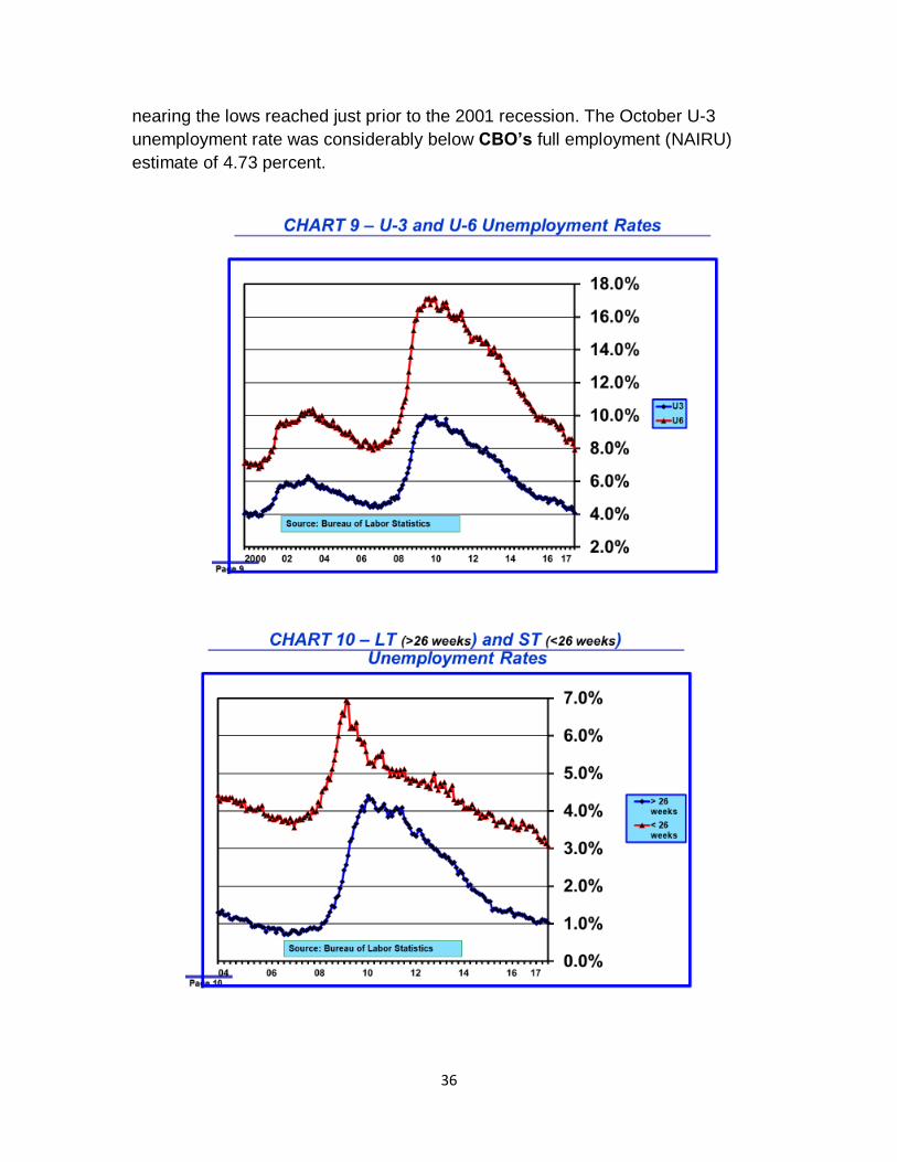
36

nearing the lows reached just prior to the 2001 recession. The October U-3 unemployment rate was considerably below CBO’s full employment (NAIRU) estimate of 4.73 percent.

37

The U-6 measure of unemployment, which adds those working part time who would prefer full-time employment and those marginally attached to the labor force to the U-3 measure, has fallen to 7.91 percent and nearly matches the pre-Great Recession low of 7.92 percent reached in December 2006. The U-6 measure of unemployment fell 199 basis points since the end of 2015 compared to a decline of 95 basis points in the U-3 measure, which underscores an improving labor market that is now above full employment.

Long-term and short-term unemployment rates are also indicators of labor market tightness and are shown in Chart 10. The short-term unemployment rate has now fallen well below the minimum level reached prior to the Great Recession. The long-term unemployment rate has declined from over 4 percent in the aftermath of the Great Recession to 1.02 percent in October. It is still about 0.30 percent above the minimum level reached in 2006 just prior to the onset of the Great Recession.

4. Forecasts of the U-3 Unemployment Rate

Forecasters expect the labor market to continue to tighten. The current U-3 unemployment rate is 66 basis points below CBO’s full-employment estimate of the non-accelerating inflation rate of unemployment (NAIRU).

As the term NAIRU implies, when unemployment falls below this level for any length of time not only is it likely that wages will increase but inflation will probably increase as well. For that reason, the FOMC is now crafting monetary policy to maintain full employment but limit the potential for tight labor markets to foster inflation. The traditional monetary policy tool involves raising interest rates. Recent indications of stronger economic growth both domestically and globally have emboldened the FOMC to “normalize” monetary policy more rapidly. However, the recent decline in inflation may delay implementation of tighter policy.

Chart 11 shows U-3 unemployment rate forecasts for B of A, GS, FOMC high and low range, and my “BASE” and “Strong Growth” scenarios. CBO’s estimate of NAIRU is also shown in Chart 11.

Most forecasts project the unemployment rate to stay below NAIRU over the next three years. GS is particularly optimistic. It forecasts that the unemployment rate will fall to 3.5 percent by early 2019. B of A expects the unemployment rate to bottom at 4.0 percent in 2018 and then begin rising gradually in 2019. Given that October’s unemployment rate is already down to 4.07 percent, it is quite possible that forecasters will have cut the estimates even further.

My unemployment rate forecasts (“BASE” scenario 4.22 percent) and CBO’s (4.18 percent) bottom in 2018. October’s rate is already below those estimates. It is now

38

evident that the unemployment rate will probably stay below CBO’s forecast for a period of time. Thus, when CBO updates its economic forecasts in early 2018 there is an increasing possibility that it will lower its forecast for the unemployment rate. That would also reduce my forecasts because my “BASE” scenario employment growth projections purposely track CBO’s. In addition, there is an increasing possibility that CBO will reduce its estimate of the NAIRU unemployment rate.

During 2019 and 2020 various forecasts diverge considerably. GS is the most optimistic. Its forecast unemployment rate forecast remains anchored at 3.5 percent and then rises to 3.7 percent in 2021. B of A expects the unemployment rate to rise from 4.0 to 4.4 percent by the end of 2020. CBO is even more pessimistic and expects the unemployment rate to reach 4.85 percent by the end of 2020. CBO’s pessimism might be tempered when it updates its employment growth assumptions in early 2018.

The upper portion of FOMC’s projection range and my unemployment rate forecasts are similar to B of A’s forecasts during 2019. My “BASE” scenario rises to 4.37 percent and my “Strong Growth’ scenario edges up to 4.15 percent by the end of 2020.

After 2019 most forecasts, with the exceptions of GS’s, including the FOMC’s long-run projected range, move upwards gradually toward CBO’s NAIRU. CBO also expects the unemployment rate to begin rising in 2019 and its forecast exceeds its estimate of NAIRU by the end of 2020.

39

Increasingly, it appears that structural changes in the labor market may have lowered NAIRU to a greater extent than indicated by CBO’s estimates. The implication of a lower NAIRU is straightforward – the labor market is not quite as tight as believed. To the extent that this turns out to be the case there will be less upward pressure on wages and inflation and the FOMC could slow the rate at which the federal funds rate is normalized. While financial markets seem inclined toward this view, the FOMC remains on a course to raise the federal funds rate much more than financial markets currently expect.

5. As the Labor Market Has Tightened, Wage Growth Has Accelerated Less Than Expected

Now that the labor market is above full employment, theory and past experience indicate that growth in wages should be accelerating. That is what is supposed to happen when excess supply disappears and demand is increasing. The data indicate this is occurring but to a more limited extent than past experience implies.

Historically, there has been considerable inertia in wage adjustments which has resulted in a slow rise in average wages even after the labor market has reached or exceeded full employment. Inertia may be greater in this cycle than previously for several reasons. First, collective bargaining power provided by unions on the behalf of labor continues to decline as a catalyst for higher wages. Second, because wage increases might not have slowed as much as they could have during the extended period of labor market slack, there may be less pressure to increase wages as much now that the labor market has tightened. Third, lingering employee long-term job insecurity may be dampening demands for higher wages. Responses to a University of Michigan survey question addressing concerns about layoff risk over the next five years remain elevated. Also, the long-term unemployment rate remains elevated. Fourth, falling inflation expectations may also be a factor. Fifth, retirement of high-wage baby boomers and replacement with low-wage new entrants may be depressing the average level of wage rates, which would moderate the average rate of wage increases. Sixth, there may be more capacity in the labor market than CBO’s NAIRU unemployment rate implies, if NAIRU has declined. The FOMC’s Summary of Economic Projections implies a median estimate of NAIRU of 4.6% and the median estimate from the Survey of Professional Forecasters is 4.5 percent compared to CBO’s estimate of 4.73 percent.6 Seventh, low productivity gains in recent years may also be a factor in retarding wage rate acceleration.

6 Regis Barnichon and Christian Matthes. “The Natural Rate of Unemployment over the Past 100 Years,” Federal Reserve Bank of San Francisco Economic Letter, 2017-23, August 14, 2017. In this paper, the authors conclude that NAIRU has fluctuated within a tight band of 4.5 percent to 5.5 percent over the past 100 years. The authors’ estimate of the current level of NAIRU is close to the lower bound of this range.

40

On the other hand, however, some of the historical inertia appears to have been offset as many states and local governments have raised minimum wage floors over the past two years.

Interestingly, the University of Michigan survey indicates that the share of workers who have not received a pay increase over the previous 12 months has been edging up and remains above the highest level that occurred following the dot.com bust in 2001.

As can be seen in Chart 12, increases in wage growth are following the traditional upward cyclical trend as the labor market tightens. But those increases are not as great as historical experience indicates should be occurring. Consequently, forecasts of wage rate increases, which have been based largely upon historical relationships, have been consistently higher than have actually materialized.

There are three primary broad-based measures of labor compensation that provide information about compensation trends. All are compiled by the Bureau of Labor Statistics (BLS). One is released monthly as part of the monthly labor situation report and includes both hourly and weekly wage rates for all employees and separately for production and nonsupervisory workers, but includes no information about benefits which comprise approximately 30 percent of total compensation. A second measure, the employment cost index (ECI), is released quarterly and consists of wages and salaries, benefits, and total compensation indices (see Chart

41

12). A third measure is also released quarterly as part of BLS’s report on output, total hours worked, and productivity.

Chart 12 shows the rate of growth in hourly wages for all workers, production and nonsupervisory workers, and ECI (total wages and salaries). All three sets of measures in Chart 12 track each other closely over time. All three measures had been rising gradually, but growth has stalled over the past few months for the all workers measure and has edged down for ECI and production and nonsupervisory workers, even as the unemployment rate has fallen well below NAIRU.

Although these measures are highly correlated over time, because compilation methodologies differ for each set percentage changes over fixed time periods will not always be in sync. Currently, all three sets are exhibiting a similar level and trend. Average hourly wages (12-month moving average) of all employees have risen 2.62 percent annually over the past 12 months compared to 2.54 percent a year ago. Increases in average hourly wages (12-month moving average) of production and nonsupervisory workers have edged down a little, rising 2.39 percent annually in October compared to 2.47 percent a year ago. ECI growth in wages and salaries has risen from 2.21 percent in the third quarter of 2016 (4-quarter moving average) to 2.40 percent in the third quarter of 2017.

To a certain extent, focusing only on hourly wages is a bit misleading. Growth in average weekly earnings for all employees, which factors in the length of the workweek and thus incorporates changes in the mix of full and part-time employees,

42

has been faster than growth in hourly wages, rising from 2.17 percent in October 2016 to 2.52 percent in October 2017 (see Chart 13). This outcome reflects a modest slowing in the average length of the workweek from 34.43 hours in September 2016 to 34.39 hours in September 2017. In fact, the average length of the workweek has edged up very slightly since the start of 2017, which could be due to stabilization in the proportions of part-time and full-time workers. Until recently, the proportion of part-time workers had been increasing.

Chart 14 shows CBO’s, GS’s and B of A’s projections for growth in the wages and salaries component of ECI for all workers and my projections for wage growth for production and nonsupervisory workers over the next ten years.

CBO, GS and B of A forecast wage rate growth only for ECI. Although the methodologies for constructing these different wage data series differ, the directionality of all is highly correlated over time, even if the levels aren’t precisely the same at every point in time. GS’s ECI wage growth forecast rises to 3.0 to 3.25 percent by 2018 and remains at that level thereafter. B of A’s ECI forecast rises to 3.3 percent in 2019 but then recedes to 3.0 percent. CBO’s ECI forecast rises to 3.4 percent in 2019 but then slows to 3.1 percent by 2021.

Forecast wage growth for production and nonsupervisory workers rises at about the same rate as CBO’s and GS’s projections in my “BASE” and “Strong Growth” scenarios, reaching 3.25 – 3.30 percent in 2019. Thereafter wage growth in my

43

“BASE” scenario tracks CBO’s and GS’s projections closely and is not much higher than B of A’s projections.

However, wage growth continues to accelerate gradually in my “Strong Growth” scenario to 3.95 percent by 2027, reflecting the impacts of faster employment growth, an extraordinarily low unemployment rate of 3.5 percent by 2027 and an extremely tight labor market with a positive gap of approximately 0.9 percent by 2027. Although this scenario is theoretically possible, it is unlikely to occur. The sharp increase in wage growth reflects strengthening wage bargaining power due to the excess of labor demand relative to supply and also greater increases in inflation. If, however, there has been a structural shift in the labor market which has decreased NAIRU, then my model would not project such a large increase in wage growth in the “Strong Growth” scenario. For example, if NAIRU is 4.5 percent, wage growth would peak at 3.7 percent in 2027 instead of 3.95 percent.

GS’s wage tracker registered 2.8 percent in October 2017, about 25 to 50 basis points short of its long-run expected 3.0 – 3.25 percent annual rate of increase. GS’s assumes a 3.8 percent unemployment rate, which is well below NAIRU, 2.0 percent inflation, and 1.0 – 1.25 percent annual productivity increases (nonfarm productivity increases would be higher, about 1.4 – 1.7 percent, as the measure of productivity GS cites does not cover the entire economy).

In GS’s view the recent weakness in wage growth results from inflation and productivity below expected long-run values. In other words, the historical forces determining wage rate growth have not changed. The upward adjustment in wage rate growth will be consistent with historical precedent and levels of the key determinants – inflation, productivity, and labor market slack. GS corroborates its view by demonstrating that low unemployment metropolitan statistical areas have experienced faster wage growth acceleration in recent months than high unemployment areas.

GS also compared the recent Federal Reserve’s Beige Book wage information with the Beige Books for 1997 and 2006, which were also times when the economy was at full employment. GS examined “labor market tightness,” “labor market conditions,” and “wage pressures.” GS concluded that the Beige Book assessment of three of these three labor market dimensions is similar to 1997 and 2006 and in both of the previous cycles, wage growth accelerated in the following year.7

7 Spencer Hill. “Quantifying Wage Signals in the Beige Book,” US Daily, Goldman Sachs Economic Research, October 4, 2017.

44

GS also recently refined its statistical “wage tracker,” which boosted its third quarter wage tracker estimate from 2.4 percent to 2.8 percent.8

While GS is sticking to its guns, others are less certain that wage rate growth will accelerate nearly as much.

6. Modeling the Relationship Between Labor Market Tightness and Wage Growth

Economic theory posits that when the demand for labor increases relative to the available supply, wage rates should rise more rapidly. This theoretical concept is embedded in the Phillips Curve. The Phillips Curve defines a statistical relationship in which decreases in the unemployment rate, improvements in productivity and increases in inflation should increase nominal wage growth. A recent GS study using city-level data confirmed the reasonableness of the Phillips Curve theoretical framework.9

In recent months, the labor market has tightened considerably and the unemployment rate is well below NAIRU. However, increases in wage rates have been muted. This has led to speculation about whether the Phillips Curve is dead.

As can be seen in Chart 14, analysts, including myself, expect wage growth to accelerate and this acceleration should occur in the next few quarters. These forecasts are based on a Phillips Curve model of wage rate behavior which by and large fits the historical data well. In other words, the Phillips Curve is not dead. The apparent slow response of wage rates to the tightening labor market can be explained by time lags between cause and effect and non-linearities in the relationship labor market variable and wage growth, which are fully visible in the historical data and which are likely to guide acceleration in wage rates in the current cycle in coming quarters.

My statistical estimation of nominal wage rate growth is based upon the following labor variables: short-term unemployment of less than 26 weeks, long-term unemployment of 26 weeks or more, the gap between the U-3 unemployment rate and CBO’s NAIRU rate, the rate of growth in total hours worked, and the square of total hours worked to incorporate a possible nonlinear relationship between nominal wage rate growth and the strength of the labor market. The model also includes the other two standard Phillips Curve variables – nonfarm productivity and core PCE inflation.

8 Jan Hatzius, Dann Struyven, and Avisha Thakkar. “Are Wages Reaccelerating?” US Daily, Goldman Sachs Economic Research, October 11, 2017. 9 Dann Struyven. “Will the Phillips Curve Bend or Break?” US Daily, Goldman Sachs Economic Research, October 17, 2017.

45

Table 9 shows the coefficients of these variables which specify the relationship between each variable, holding the impacts of all other variables constant, and the nominal wage rate. Average time lags measured in months for each variable are also shown in Table 9.

As short-term and long-term unemployment rates rise and labor market slack expands, increases in nominal wage rates decline. The impact of a change in the short-term unemployment rate is greater and affects the nominal rate more quickly than a change in the long-term unemployment rate. A tightening in labor market slack of 1 percentage point raises nominal wage rates by 1.24 percent in an average of 16.7 months.

Table 9

Nominal Wage Rates – Impacts of Labor Market Variables, Productivity and Core PCE Inflation

Coefficient

Average Lag (in months)

ST Unemp. Rate < 26 weeks -2.02 15.5 LT Unemp. Rate >26 weeks -1.26 43.9 Labor Market Gap -1.24 16.7 Growth in Hours Worked 0.86 23.7 Growth in Hours Worked^2 2.93 Productivity 0.30 47.7 Core PCE Inflation 0.82 12.5

Growth in total hours worked raises the nominal wage rate, but its incremental effect is nonlinear as can be seen in Table 10. The average lag time between cause and effect is about 2 years (23.7 months), which explains in part the apparent slow response of nominal wage rate increases to acceleration in employment market growth.

Core PCE inflation impacts the nominal wage rate with an average lag of about one year (12.5 months). A one percentage point increase in core PCE inflation lifts nominal wage rate growth by 82 basis points. Once the labor market has tightened sufficiently, there is probably a positive feedback loop between the increase in the nominal wage rate and changes in inflation, but the statistical analysis indicates that increases in the wage rate lag behind and depend on increases in inflation to occur first.

46

Table 10

Incremental Impact of Growth in Total Labor Hours Worked on Nominal Wage Rates

Growth in Total Labor Hours Worked

Incremental Impact on Nominal Wage Rate Growth

3.0% 2.84% 2.0% 1.83% 1.0% 0.89% 0.0% 0.00% -1.0% -0.83% -2.0% -1.60% -3.0% -2.31%

Finally, while productivity does have a positive impact on the nominal wage rate, it is smaller than most believe and takes a long-time to have even this small impact. A one percentage point increase in nonfarm productivity raises the nominal wage rate by 30 basis points but this takes an average of 4 years (47.7 months) to occur.

You can see in Chart 14 how a very tight labor market sustained over time, as is the case in the “Strong Growth” scenario, can result in a much higher rate of increase in the nominal wage rate.

Although my econometric model describes well the historical relationships between nominal wage rate growth and the economic variables in the Phillips Curve, over the past few months the model overestimated the rate of increase in the nominal wage rate and that error reached the 2-standard deviation level in October. This is too recent a phenomenon to conclude that the historical relationship is breaking down. However, the model indicates that the inflection point is at hand when growth in the nominal wage rate should accelerate. This is evident in Chart 14. If the nominal wage rate does not accelerate in the next few months and the close the forecasting error gap, then it will be time to reconsider whether there really has been a structural change in the historical Phillips Curve.

This is not a trivial matter. If wage rate growth is poised to accelerate, as the model predicts, the FOMC should continue to raise the federal funds rate to contain a buildup in inflationary pressures. However, if wage growth does not accelerate meaningfully, an overly aggressive monetary policy could hasten onset of recession.

47

7. Impact of 2 Percent Inflation on Nominal Wage Growth Rate

Chart 15 shows two alternative nominal wage rate growth curves – one for my forecasts of the core PCE inflation rate and an alternative one in which core PCE inflation is assumed to be constant at the FOMC’s target of 2.0 percent.

Because my forecast of core PCE inflation averages less than 2.0 percent, my forecasts for nominal wage growth rate average 30 basis points less in the “BASE” scenario – about an average annual rate of increase of 3.26 percent between 2021 and 2027 compared to 3.57 percent if inflation averages 2.0 percent. My “BASE” scenario parallels GS’s long-term 3.25 percent and CBO’s long-term 3.12 percent rates of increase.

VI. Inflation

Surprising just about everyone, core PCE inflation has declined this year even as unemployment fell below NAIRU. This has led to much head scratching. Nonetheless, most FOMC members remain confident that both core and total PCE inflation will return to the 2.0 percent target level by 2019.

1. Inflation Trends

When core PCE inflation was 1.87 percent in 2016 and appeared to be well on the way to reaching 2.0 percent, FOMC members were confident that the target of 2.0 percent would be reached in the next two years. However, core inflation has

48

declined steadily since February and stood at 1.33 percent in September and was not much different from its recent low of 1.25 percent in July 2015. Initially, FOMC members dismissed the pullback in inflation to transitory factors, but the persistent decline over several months has led some members to worry about the possibility that inflation expectations have become unanchored to the downside.

Total PCE inflation, which had been depressed by the plunge in oil prices and lower import prices in late 2015, rebounded to 2.18 percent in February, up from the 0.19 percent rate of increase that prevailed in September 2015. But total PCE inflation has declined since then and was 1.63 percent in September.

As can be seen in Table 11 (Chart 16 shows historical core PCE price index data and data from Table 11 in graphical form), forecasts of the core PCE inflation index now indicate that inflation will be lower in 2017 than in 2016. Over the longer run, B of A expects core PCE inflation to settle at the FOMC’s 2.0 percent target. GS is forecasting 2.1 percent in 2019 and 2.2 percent in 2020 before dropping back to 2.0 percent in following years. CBO projects that 2.0 percent is reached by the end of 2018 and remains at that level thereafter. FOMC projections reflect a rise to the 2.0 percent target during 2018 or 2019.

Table 11

Core PCE Inflation Forecasts – B of A, GS, Bill’s “BASE”, Bill’s “Strong Growth” and FOMC High and Low

Core CPE 2013

2014

2015

2016

2017 2018 2019 2020 2021

Actual 1.55 1.48 1.37 1.87 B of A 1.41 1.79 2.02 2.02 2.02 GS 1.40 1.80 1.90 2.10 2.10 CBO 1.77 1.97 1.99 2.01 1.99 IHS Markit* 2.10 1.70 2.20 2.70 2.40 Economy.com* 2.00 2.10 2.80 Blue Chip Average* 2.10 1.90 2.30 2.30 2.30 Bill’s BASE 1.53 1.89 1.85 1.68 1.55 Bill’s Strong Growth

1.53 1.93 1.98 1.82 1.72

FOMC – High 1.6 2.0 2.0 2.1 2.0 FOMC – Low 1.5 1.8 2.0 2.0

*CPI – total index; on average CPI averages about 25 basis points higher than CPE

Part of the unexpected recent softness in core PCE inflation is related to quality improvements in cell phones, but other price categories, such as shelter and medical services inflation, have been weaker than expected.

49

As can be seen in Chart 16, my econometric model indicates core PCE inflation will closely track the estimates of others through 2020, but softens in 2021. During 2018, 2019, and 2020 core PCE inflation forecasts in the “BASE” and “Strong Growth” scenarios are just shy of 2.0 percent but then decline in 2021 and remain slightly below 2.0 percent thereafter, reaching 1.6 percent (“BASE”) to 1.9 percent (“Strong Growth”) by 2027.

Chart 17 shows core PCE inflation estimates for my “BASE” and “Strong Growth” scenarios from 2017 to 2027. What is notable in Chart 17 is that inflation moves up to the FOMC’s 2.0 percent target in 2018 and 2019 but in the “BASE” scenario falls well below that target after that.

While one should never discount the possibility of a sea-change in the economic environment in the future that would set inflation on a different course, there are good reasons to conclude that core PCE inflation may remain modestly below 2.0 percent in coming years, notwithstanding an economy that is operating at full employment and which might benefit from additional fiscal stimulus in the coming year.

50

2. Drivers of Inflation

There are many drivers of inflation, which can be sorted roughly into three groups – (a) fundamental macro forces, (b) policy influences, and (c) other drivers which do not fit neatly into the other two categories. Like all matters in economics, the directional contributions of each driver in theory can be posited, but on a real-time basis these drivers interact with each other in complex ways which make it difficult to forecast inflation with precision.

a. Macro Forces

Domestic Demand and Supply. This force is the most significant one. Simply put, as demand increases relative to supply, prices rise to clear the market. This is true for specific products and services. It also is true for the relationship between the aggregate price level and the output gap. As the output gap diminishes, the aggregate price level rises.

At the aggregate level, there is evidence that the relationship between inflation and the output gap is nonlinear. As the size of the output gap rises, prices fall but at a decelerating rate. As the output gap narrows or turns positive (actual output exceeds its non-inflationary potential) prices rise at an accelerating rate.

In my econometric model, I capture the effects of demand and supply on aggregate inflation, through three variables – the U-3 unemployment rate, and the employment gap measured as the difference between CBO’s nonaccelerating inflation rate of

51

unemployment (NAIRU) and the U-3 unemployment rate. The third variable introduces nonlinearity into the model by squaring the measure of the labor gap. As the size of the labor gap increases, inflation falls as expected but the impact is nonlinear.

Wealth. Increases in wealth bolster demand and in so doing place upward pressure on inflation. The two main components of wealth consist of financial instruments and real assets such as housing. In my econometric model, a one percentage point increase in the rate of residential housing appreciation is associated with a 0.23 percentage point increase in core PCE inflation.

Dollar’s Value and International Competition. Many factors influence the value of the dollar. In general, an increase in the value of the dollar makes imports less expensive and exports more expensive. In the aggregate, this has a negative effect on domestic demand and places downward pressure on inflation. In my econometric model, a one percentage point increase in the trade-weighted dollar index sustained for one year reduces core PCE inflation by 4.4 basis points.

In recent years, the rapid development of emerging economies, especially China, has increased the global supply of inexpensive goods relative to global demand. This is a strongly deflationary development and is reflected in low inflation and low interest rates worldwide. However, GS argues that the impact of cheap imports on U.S. inflation peaked in the late 1990s and early 2000s.

Productivity. Improvements in production efficiency increase the supply of goods and services relative to demand. Thus, increases in productivity place downward pressure on inflation. In my econometric model, a one percentage point increase in productivity is associated with a 35 basis point reduction in the level of core PCE inflation. Unfortunately, productivity growth in recent years has been rather dismal, which means that the lack of productivity has placed upward pressure on inflation.

Of course, if productivity were to improve significantly going forward, this development would hold inflation down. The Amazon effect on retailing productivity and the Verizon effect on communications productivity are cited as examples of potential productivity increases. However, the Amazon effect is not yet meaningful, and the recent Verizon effect in reducing the core PCE price index this year may prove to be a one-time idiosyncratic adjustment rather than the beginning of sustained downward pressure on core PCE inflation from steady improvements in communications technology.

52

b. Policy Influences

Monetary Policy. In theory, properly administered, monetary policy should have only transitory impacts on inflation as central banks adjust policy to stimulate aggregate demand and employment or to slow aggregate demand and employment to limit upside pressure on inflation. However, a sustained overly stimulative monetary policy can unleash the inflation gremlin – too much money chasing too few goods and services. Conversely, a sustained overly tight monetary policy can lead to deflation.

Regulatory Policy. Regulatory policy can have either favorable or unfavorable impacts on inflation. An example of favorable effects would be rules and processes that discourage fraud and bribery and anchor the efficacy of the rule of law. But, rules and regulations can also result in unproductive costs of doing business and can impede competition. Sometimes it is difficult to sort out the pluses and minuses of the effects of regulation on inflation. Licensing requirements, for example, can keep crooks out but can also limit competition.

Other governmental programs and policies, especially in the area of healthcare, can have significant impacts on inflation. Some of the recent decline in core PCE inflation can be traced to price controls contained in the Affordable Care Act.

Market Structure. Systematic and persistent significant structural changes in the economy impact inflation. Two examples illustrate the potential impacts. First, business concentration has increased in recent years. Theory posits that increases in concentration impart pricing power which leads to higher inflation. However, offsetting this is that more of revenue flows to owners than workers, which results in weaker wage growth and less pressure on inflation. In addition, increases in concentration also discourage new business formation and this phenomenon tends to be linked with lower productivity gains and less downward pressure on inflation. Thus, increasing concentration has multiple impacts on inflation and it is unclear what the aggregate net effect is.

Second, some argue that the decline in unions, by decreasing labor bargaining power, has contributed to lower inflation.

c. Other Drivers

Demographics. Population growth slows as countries develop economically. This is now a widespread global phenomenon. It is argued that slower population growth places downward pressure on inflation as an aging population shifts from an emphasis on consumption to saving. However, this phenomenon is offset by escalating health care costs that crescendo as the overall population ages.

53

Research does not find that an aging population has a significant impact on inflation. GS did some statistical work and found that an aging population in the U.S. has decreased the level of inflation since 1980 by only 5 basis points. In my own work I found an opposite effect which is not significant – a one percentage point decrease in employment growth (proxy for population growth) is associated with a one basis point increase in inflation.

Income and Wealth Inequality. Income and wealth inequality in the U.S. has worsened over the past 40 years. Because lower income people have a higher propensity to consume out of their income, it is argued that widening income inequality puts downward pressure on aggregate demand which, in turn, lessens upward pressure on inflation.

3. Measurement Challenges

GS presents analysis that supports its view that this year’s decline in inflation is due to idiosyncratic developments which will not persist. GS sorted 51 inflation components into two groups – those that are well measured and those that are easily susceptible to measurement error.10 Inflation in the well-measured components is 1.6 percent and is unchanged this year. The weakness in inflation during 2017 is concentrated in the hard to measure components, which include communications, medical services, owners’ equivalent rent, apparel, and lodging. In addition, GS observes that cyclical index components have edged up as the output gap has diminished as would be expected.11 Overall, GS believes that their analysis supports its view that inflation will move upward toward the FOMC’s 2 percent target over the next two years.

There are several alternative inflation indices that have been constructed to attempt to tease out underlying inflation trends which are obscured by idiosyncratic noise. One such index which has received notice recently is the New York Federal Reserve Bank’s CPI Underlying Inflation Gauge. This index indicates that trend inflation is accelerating. Most alternative inflation indices attempt to cull out volatile components such as the Cleveland Federal Reserve Bank’s weighted-median and trimmed-mean CPI. The New York Federal Reserve Bank’s methodology differs in that it uses a dynamic factor statistical methodology to tease out the long run trend embedded in 223 individual price series. This methodology indicated that trend CPI inflation in August was 2.2 percent compared to reported total CPI inflation of 1.9 percent in the same month.

10 Spencer Hill. “The Map of the Territory? Measurement Error and Low Inflation,” US Daily, Goldman Sachs Economics Research, November 17, 2017. 11 Daan Struyven. “Which Prices Still Respond to Slack?” US Daily, Goldman Sachs Economics Research, October 31, 2017.

54

4. Bottom-Up versus Top-Down Assessment of Inflation Trends

There are two ways to forecast inflation. The method I use in my econometric model is a top-down approach. A top-down approach looks at how inflation varies over time with other macroeconomic variables. This approach generally assumes that there is a stable relationship over time between inflation and other economic variables. In a dynamic economic environment, an assumption of structural stability can miss substantive changes that could lead to upward or downward bias in inflation forecasts.

An alternative way of forecasting inflation is to employ a bottom-up methodology. This involves decomposing inflation into its many components and analyzing how each component is likely to evolve over time. One can quickly get bogged down in the complexity of analyzing the behavior of dozens of prices categories. And, while it might seem that this level of granularity should overcome the bias inherent in the assumption of structural stability in the top-down approach, the bottom-up approach is not entirely free from this bias either. However, the bottom-up approach can provide additional insight into whether the simpler top-down approach is reasonable or whether it is likely to result in systematic biases over time that lead to over or underestimating inflation.

GS’s work on looking individually at cyclically-sensitive components of the inflation index and evaluating trends in well-measured components are examples of a bottoms up methodological approach.

Evaluation of significant components and assessment of their underlying trends lend credibility to the case for inflation to move back toward the FOMC’s 2 percent target over the next two years.

Financial Services. This component accounts for about half of the decline in core PCE inflation this year and involved reductions in money management fees and commissions. These adjustments are viewed as one-off and unlikely to continue.

Accommodations. This component has contribute 6 basis points to the decline in core inflation but this impact is not expected to continue.

Housing – Owners’ Equivalent Rent. This component has contributed 5 basis points to the decline in core inflation, dropping from an annual rate of 3.6 percent to 3.3 percent. This impact may continue if the incipient switch from renting to owning continues. That said, GS believes that this measure understates the cost of owning at a time when average housing prices are rising at a 6 percent clip.

55

Communications. This is the so-called Verizon effect involving one-time shift to unlimited data plan offerings. The impact of this price reduction will drop out of the index during 2018.

Healthcare. Healthcare inflation is 2 percentage points less today relative to an extrapolation of the 2000-2007 trend in healthcare inflation. About 75 basis points is traceable to price cuts mandated by the Affordable Care Act. The remainder of the decline, according to GS, is due to structural and cyclical factors that have temporarily depressed healthcare inflation to a 1.2 percent annual rate. GS expects healthcare inflation to rise to about 2.2 percent over the next few years.

Retailing. GS estimates that the Amazon effect may be reducing core goods inflation by 25 basis points and core inflation by 10 basis points. This may continue, but is not judged to be particularly significant.

5. Summary

When all is said and done, the bottom line is that core PCE inflation is likely to be near 2.0 percent over the next few years. Top-down models imply that core inflation will be a little but not much below 2.0 percent in coming years. That is consistent with the historical record. Alternative indices and granular analysis of individual inflation components suggest that inflation will rise to about 2.0 percent but not much more than that. The problem with the bottoms up approach is that it does not necessarily capture the unexpected surprises such as this year’s reduction in inflation because of price changes in wireless communications plans.

But, why worry, a small difference in inflation forecasts of 0.5 percent really shouldn’t matter a great deal in the conduct of monetary policy.

VII. Monetary Policy

Members of the Federal Open Market Committee (FOMC) have gone to considerable lengths in recent years to communicate as clearly and transparently as possible their assessment of the economy and what they collectively believe is an appropriate monetary policy to meet the twin objectives of full employment and moderate inflation.

1. Monetary Policy Making Process

FOMC members gather in Washington, DC eight times a year. At the end of each meeting the FOMC releases a statement that contains an assessment of economic activity, employment and inflation and commentary about risks to the outlook. The statement concludes with a summary about the course of monetary policy and specific actions the FOMC has decided to implement. For several years at the

56

second quarterly meeting members update their economic projections and the chairmen holds a press conference. The intent has been to provide greater transparency about the conduct of monetary policy. In recent years, it has been the practice to announce changes in monetary policy at the second quarterly meeting. Because the release of economic projections and a press conference follows this meeting, the chairman has the opportunity to explain reasons for any policy changes. As a result, the markets are rarely surprised. This has contributed to a lessening of market volatility in recent times.

However, the market keeps its own counsel and does not blindly accept indications of future policy that are embedded in FOMC member economic projections, the FOMC statement, the press conference and speeches given by Federal Reserve officials. While the market does not always agree with the FOMC’s assessment of the economic outlook and the likely course of monetary policy, it has come to trust the FOMC to update its views as new real-time information becomes available and not to blindly pursue a rigid policy agenda. At the present time, the disagreement between the market forecast for the federal funds rate and the projections of all others, included FOMC members, is unusually large. The market expects only three more increases in the federal funds rate to a range of 1.75 percent to 2.00 percent. The number of forecast increases from others range from 6.5 (FOMC median) to 9 (see Table 12).

Federal Reserve Board of Governors Chair, Janet Yellen, said in a speech to the G30 on October 15, 2017, “… we continue to expect that the ongoing strength of the labor market will warrant gradual increases in that rate [federal funds] to sustain a healthy labor market and stabilize inflation around our 2 percent longer-run objective.” Market participants collectively believe that low and declining inflation will cause the FOMC to limit the number of increases in the federal funds rate after December. Yellen pushed back on this view saying that “… my best guess is that these soft readings will not persist and with the ongoing strengthening of labor markets I expect inflation to move higher next year. Most of my colleagues on the FOMC agree.”

This guidance sounds unambiguous, but markets refuse to believe. We now know that Janet Yellen will not be Fed chair beginning in February 2018, but her replacement, Jerome Powell, who is currently Vice Chair of the Board of Governors, has consistently supported the recent approach to monetary policy and is expected to continue to stay the course. There is considerable inertia in the formulation of monetary policy, and Jerome Powell is unlikely to initiate any kind of significant monetary policy course adjustment.

57

So, the disagreement between the market and others about the level of the long-run equilibrium federal funds rate will continue and the eventual outcome will depend upon future developments.

2. Beige Book – Assessment of the Economy

Three weeks prior to each FOMC meeting, the Beige Book is published. It summarizes in anecdotal form recent economic activity in each of the 12 Federal Reserve districts. The most recent Beige Book covered the period from late August to October 6th. Overall, economic activity did not change from the previous report and is considered to be “moderate,” which means trend real GDP growth is about 2 percent. Only the Richmond regional bank upgraded its view from “modest” to “moderate.”

Labor markets are considered to be tight, but wage pressures are “subdued.” Shortages of skilled workers, particularly in manufacturing, construction, transportation, and some sectors of health care, are impeding growth. Nonetheless, there is not much evidence of increasing pressure on wages except in specific sectors such as transportation and construction.

There was no change in commentary about inflation. Essentially, there are no significant upside pressures developing. The recent increase in commodity prices was noted, but there has been limited pass through into retail prices.

3. FOMC Statement – Assessment of Economic Activity, Employment, and Inflation

There was no change in the assessment of the labor market – “… the labor market has continued to strengthen ….”

Economic activity, however, was upgraded from “… economic activity has been rising moderately so far this year” to “… economic activity has been rising at a solid rate ….”

There was no change in the inflation assessment. The statement simply acknowledged the data trends: “… inflation for items other than food and energy remained soft. On a 12-month basis, both inflation measures [total and core] have declined this year and are running below 2 percent.” Market-based measures of inflation remain low and survey-based measures of inflation expectations are stable. Although, the commentary about inflation in the statement is factual and not interpretative, Chair Yellen and other FOMC members have expressed the view that the recent decline in the PCE inflation measures is transitory and due to idiosyncratic measurement developments. Overall, FOMC members remain

58

confident that inflation will return to the 2 percent target level over the next two years.

4. FOMC Statement – Assessment of Risks

FOMC members dismissed the impacts of the recent hurricanes: “… the storms are unlikely to alter the course of the national economy over the medium term.” Thus, the policy course of “gradual adjustments in the stance of monetary policy” will be consistent with gradual improvement in economic activity and labor markets and a slow increase in inflation.

“Near-term risks to the economic outlook appear roughly balanced, but the Committee is monitoring inflation developments closely.” So, although FOMC members are confident that inflation will eventually reach the 2 percent target level, the use of the word “monitoring” acknowledges that there is some uncertainty and communicates to the market that if future data indicate that inflation is not moving up toward the target, the FOMC will adjust monetary policy.

5. FOMC Statement – Monetary Policy

As expected, the FOMC left the federal funds rate unchanged, but noted that monetary policy remains accommodative and supportive of stronger economic activity and higher inflation. The policy paragraph was identical word-for-word to the one issued after the previous FOMC meeting. In addition, the policy statement simply acknowledged that “the balance sheet normalization program” commenced in October and is proceeding.

Just as a comment about balance sheet shrinkage came at the end of the policy statement and was almost an obligatory afterthought, the market has not focused on the possible longer run implications of balance sheet shrinkage. Perhaps this is because the shrinkage will be very limited initially. But let there be no doubt that liquidity will begin to be impacted in a meaningful way. Already measures of the supply of money and credit indicate that growth is slowing and “quantitative tightening” and increases in the federal funds rate will only serve to depress growth further. Another indicator of decreasing liquidity is the narrowing of the yield spread between the 10-year and 2-year Treasury securities from 125 basis points at the beginning of the year to 62 basis points currently. The deceleration in growth of money and credit is consistent with a maturing economic cycle but has not yet reached the red zone which in previous cycles has sent a reliable signal of heightened recession risk.

59

VIII. Interest Rates

This month I revised my econometric model to accommodate better for the impact of the long period of zero short-term interest rates. The revised estimates of the federal funds rate are more reasonable in the sense that the term premium (the difference between the forecast equilibrium ten-year yield and the federal funds rate) ranges between 75 and 90 basis points, which is consistent with historical experience.

These model revisions improved the reliability of my interest-rate forecasts. Of course, the forecasts themselves depend assumptions about employment growth, labor market tightness, productivity, and inflation. This means that interest-rate forecasts depend upon a lot of assumptions, some of which or many might prove to be inaccurate. Nonetheless, for a plausible range of assumptions, the model provides a bounded range of interest-rate forecasts. Table 11 below shows how short-term and long-term interest rates can be expected to vary over time based on differences in key economic assumptions.

1. Interest Rates – Federal Funds Rate

The FOMC raised the federal funds rate 25 basis points at its June meeting to a range of 1.00 to 1.25 percent. The FOMC’s projections indicate that there will be one more increase of 25 basis points in 2017, which is likely to occur at the December meeting. Market sentiment agrees and currently assigns an 80 percent likelihood.

Table 12

Number of Federal Funds Rate Increases of 25 Basis Points

2017 2018 2019 2020 2021-27 Total Long Run

FOMC – median 3 3 2 0.5 0 8.5 2.50-3.00* B of A 3 3 3 0 0 9 2.75-3.00* GS 3 4 4 0 0 11 3.25-3.50* IHS Markit 3 3 3 1 0 10 2.75-3.25 Economy.com 3 3 5 0 0 11 3.25-3.50 Market Forecast 3 1 1 0 0 5 1.75-2.00 Bill’s BASE 3 3 1 2 -2 7 2.25-2.50# Bill’s Strong Growth 3 4 1 2 2 12 3.50-3.75# *FOMC, B of A and GS rates are equilibrium estimates #Bill’s estimates are forecasts which peak above the likely equilibrium rate

With respect to the issue of additional increases in the federal funds rate in 2018 and subsequent years, there is considerable divergence among the FOMC’s own projections, forecasts of analysts and the market forecast embedded in TIPS

60

securities. The expected number and timing of federal funds rate increases made by several analysts, including myself, the FOMC and the market is shown in Table 12.

In its September Summary of Economic Projections (SEP), the median FOMC member’s view is three 25 basis point increases in the federal funds rate in 2017 to 1.25 - 1.50 percent, two of which have already occurred; three more in 2018 to 2.00 - 2.25 percent; two more in 2019 to 2.50 - 2.75 percent; and possibly one increase in 2020 to 2.75 – 3.00 percent. The FOMC’s central tendency long-term equilibrium level for the federal funds rate is 2.50 to 3.00 percent. In the past the SEP projections have proved to be very unreliable guides to future monetary policy. For example, at the beginning of 2016 the FOMC median projected four increases in the federal funds rate during 2016. Only one occurred. While most seem to agree that 2017 will see three increases, which is not a very risky call since two increases have already occurred, there is divergence of opinion about the number of increases in 2018 and later years.

B of A and GS both expect three increases in 2017 with the remaining increase occurring in December. Over the longer run GS expects more tightening than B of A and the FOMC and a higher equilibrium level of the federal funds rate of 3.25 to 3.50 percent compared to 2.50 to 3.00 percent for the FOMC and 2.75 to 3.00 percent for B of A.

My federal funds rate forecast in my “BASE” scenario agrees with the consensus in 2017, followed by three increases in 2018, two in 2019 and one more in 2020. My “BASE” case peak rate reaches 2.75 percent in 2020 and then drifts gradually back to 2.50 percent after that. This point-estimate assumes weak productivity and inflation that does not reach the target 2.0 percent level. Also, it is not an equilibrium rate but a forecast that reflects a cyclical peak of an economy operating slightly above full capacity. My estimate of the long-term equilibrium rate ranges from 2.10 to 3.15 percent, depending upon the strength of inflation and productivity (see Table 13).

In my “Strong Growth” scenario the federal funds rate rises to a higher cyclical peak of approximately 3.75 percent by 2024. This higher projected rate reflects the consequences of a tight monetary policy in an overheated economy – the unemployment rate falls gradually to 3.5 percent in this scenario by 2027, considerably below the NAIRU rate of approximately 4.7 percent. Such a high rate is unlikely to occur because monetary policy tightening will in all likelihood slow economic growth or even result in recession long before rates rise to this high a level.

61

Chart 18 shows the quarterly progression in the federal funds rate from the present through 2021 implied by the FOMC’s high, low and average projections. It also shows forecasts for B of A, GS, my “BASE” scenario and the market forecast embedded in federal funds futures. My forecast pathway is in the middle of the pack. GS is a bit more pessimistic than most other forecasters. The market forecast is much lower than all other forecasts any tops out in a range of 1.75 percent to 2.00 percent in 2019.

Until December 2016, FOMC members had steadily reduced the median estimate of the long-term nominal value of the federal funds rate from 4.25 percent to its current range of 2.50 to 3.00 percent. Based upon my model, my sense is that the FOMC’s median projection for the federal funds rate is reasonable with its estimate of long-term real GDP growth of 1.8 to 2.0 percent. My “BASE” scenario, assuming 2.0 percent core PCE inflation, indicates that a long-term nominal federal funds rate of about 2.85 to 3.15 percent is a likely range for the long-term neutral federal funds rate, but it could be lower, if productivity remains relatively weak and inflation is lower. This also means that the real neutral interest rate, assuming inflation is 2.00 percent, would be .85 to 1.15 percent. (See Table 13.)

2. Interest Rates – 10-Year Treasury Note Yield

Chart 19 shows forecasts for the 10-year Treasury note yield over the next ten years. Over time analysts have reduced their forecasts for the ten-year yield. Partly

62

this is a mark-to-market exercise driven by the persistent decline in this yield contrary to expected increases. But the adjustments also reflect a growing consensus that the long-run equilibrium real rate of interest has declined. Analysts still expect long-term rates to rise from the current level, but no longer to as high a level.

Assuming an inflation rate of 2.0 percent, my model indicates that the 10-year neutral rate should be between 3.50 percent and 4.00 percent, depending on the level of productivity. (See Table 13.) The long-term neutral rate is 3.60 percent for GS, 3.25 percent for B of A and 3.70 percent for CBO. These estimates do not differ materially from my estimated range of 3.50 percent to 4.00 percent.

My forecasts for the 10-year yield in my “BASE” scenario, which are shown in Chart 19, are lower in the long run (2025-2027) than those of most other forecasters, with the exception of B of A, because my forecasts of inflation are lower than 2.0 percent. The range in my average annual forecasts is 3.40 to 3.65 percent between 2021 and 2027, rather than 4.05 to 4.30 percent that my model says would prevail if inflation were 2.0 percent in the “BASE” scenario.

3. Real Rate of Interest and Natural Rate of Interest

The real rate of interest is the nominal rate of interest minus the rate of inflation. Over the economic cycle both the nominal rate of interest and the reported inflation rate vary. Thus, the real rate of interest also varies over the cycle.

63

The natural rate of interest, sometimes also referred to as the neutral rate of interest or the equilibrium rate of interest, is a specific value of the real rate of interest (nominal rate of interest less the monetary authority’s target inflation rate) that occurs when an economy is operating at (not below or above, but at) its full potential. The value of the natural rate depends upon fundamental factors such as the rate of population growth, demographics (e.g., aging), productivity, and inflation expectations. Because these fundamental factors do not necessarily remain constant over time the value of the natural rate can vary.

The natural rate is not directly observable and thus has to be teased out of messy data.

From a monetary policy perspective, the importance of knowing the value of the natural rate of interest involves determining, when the monetary authority’s inflation target rate is added, what the nominal value of the short-term interest rate – the federal funds rate – will be when the economy is operating at full capacity.

In the FOMC’s Summary of Economic Projections (SEP), one of the data points members supply is an estimate of the long-run equilibrium federal funds rate. This is the same as the neutral or equilibrium rate of interest because the accepted assumption is that it is the rate that will prevail when the economy is operating at full capacity. In the September SEP the central tendency range for this rate was 2.50 to 3.00 percent. Given that the FOMC’s inflation target is 2.0 percent, this means that the consensus of FOMC members believes that the neutral rate of interest is in a range of .50 to 1.00 percent.

This all seems to be very tidy. However, there are two big assumptions embedded in the long-run SEP equilibrium value of the federal funds rate. First, and obviously, is that the real rate of interest when the economy is operating at full capacity will be in a range of .50 to 1.00 percent. Second, and less obviously, is that the FOMC will be successful in achieving a 2.0 percent stable nominal inflation rate. Most assume that the FOMC has the power to engineer such an outcome. But, neither assumption is absolutely guaranteed. Both could be wrong.

What evidence exists suggests that both of the FOMC’s assumptions for the real rate of interest and inflation, when the economy is operating at full capacity, could be too high. Certainly, this is what the market believes currently. The market currently expects at most another 50 basis points increase in the federal funds rate to a range of 1.50 to 1.75 percent. This is 100 basis points lower than what the FOMC and most analysts, including myself, project, which is a very large and significant difference. Of course, the market could be wrong and the FOMC right; or vice versa, or “truth” could lie somewhere in between.

64

This is not a trivial issue. If the FOMC sticks to its guns and believes it knows best and forges ahead, but the market’s assessment is the more correct one, the FOMC will commit a serious policy error by over tightening monetary policy and this will surely push the U.S. economy into recession.

There is no clear-cut answer to who is correct or closer to being correct. But, because the consequence of an overaggressive monetary policy – recession – is greater than the consequence of too easy a monetary policy – economic overheating and higher inflation – good risk management principles argue for a more cautious monetary tightening approach than is currently spelled out in the FOMC’s SEP. If inflation remains subdued and far short of the 2.0 percent target, expect the FOMC in the future to revise down its projections for the federal funds rate, even if the unemployment rate continues to fall.

4. BASE Scenario Estimates of Nominal and Real Short-Term and Long-Term Federal Funds and 10-Year Treasury Rates

My econometric model provides estimates of values of the short-term (2017) and long-term (2021-27) federal funds rate and the 10-year Treasury rate.

Estimates are shown in Table 13 for various assumed values of inflation, the growth rate in total hours worked and productivity. The estimates are based upon a key assumption that the economy is operating at full capacity, whatever are the assumed levels of inflation, employment growth and productivity. In other words, for a specific set of assumptions about inflation, employment growth and inflation, the model estimates the equilibrium nominal interest rates for that set of assumptions.

As such, the implied real rate of interest can be deduced by subtracting the long-run stable value of inflation from the estimate of the nominal federal funds rate. There is a long-term equilibrium value of the real rate of interest for each set of economic assumptions. However, since there are many possible sets of economic assumptions, it follows that there are many possible values for the long-term equilibrium real rate of interest. In other words, the real rate of interest is not a static value but varies in predictable ways with changes in key economic variables.

Theory postulates that the real rate of interest rises with greater employment growth, increases in productivity and higher inflation. The model estimates of nominal rates of interest, inflation and implied real rates of interest are consistent with theory.

My estimates of the long-term federal funds rate are more consistent with the FOMC’s SEP projections than with current market expectations. As can be seen in Table 13, if inflation averages 2.0 percent, my estimate of the long-run real rate of interest is in a range of .83 to 1.17 percent, depending upon the strength of

65

productivity, compared with the FOMC’s estimated range of .50 to 1.00 percent for the neutral rate. Notice that if inflation averages 1.57 percent rather than 2.00 percent, the real rate of interest is about 30 basis points lower and ranges from .52 percent to .82 percent, which is solidly within the FOMC’s estimated range for the neutral real rate of interest.

Table 13

Short-Term and Long-Term Interest Rates for Federal Funds and 10-Year Treasury Rates (BASE Scenario)

Short-Term (2017)

Assumptions

Long-Term Assumptions (2021-27)

Potential Real GDP 1.58% 1.35% 1.78% 1.95% Inflation (core PCE) 1.62% 2.00% 2.00% 2.00% Productivity .80% .90% 1.40% 1.60% Labor Force 1.92% .60% .60% .60% Nominal Rate Federal Funds 1.21% 2.83% 3.08% 3.17% 10-Year Treasury 2.60% 3.49% 3.85% 3.99% Implied Real Rate Federal Funds -.41% .83% 1.08% 1.17% 10-Year Treasury .98% 1.49% 1.85% 1.99% Long-Term Assumptions

(2021-27) Inflation (core PCE) 1.57% 1.57% 1.57% Productivity .90% 1.40% 1.60% Labor Force .60% .60% .60% Nominal Rate Federal Funds 2.09% 2.34% 2.44% 10-Year Treasury 2.86% 3.22% 3.36% Implied Real Rate Federal Funds .52% .77% .87% 10-Year Treasury 1.29% 1.65% 1.79%

In the top panel of Table 13 it is assumed that growth in total hours worked remains constant at 0.6 percent annually in the long term and that core inflation remains anchored at 2.0 percent and shows the impact on the federal funds and the 10-year Treasury rates for assumed productivity values of 0.9, 1.4, and 1.6 percent. The only change in the bottom panel of Table 13 involves substituting my forecast of core inflation, which averages 1.57 percent over the 2021-27 period, for an assumed target rate of 2.0 percent.

66

IX. Fiscal Policy – All Eyes on Congress and the Possibility of Tax Reform and Cuts

Congress has been busy working on tax reform legislation. On November 16th, the House of Representatives passed the “Tax Cuts and Jobs Act” by a vote of 227-205 with 13 Republicans and all Democrats voting no. The Republican “No’s” were all from states which are considered to be “blue” and which would be especially hard hit by repeal of the state and local income tax deduction. At the same time, the Senate Committee on Finance was working feverishly on an alternative tax reform bill.

While some remain skeptical about congressional action on tax reform, GS has raised its odds of enactment to 80 percent and has revised its economic forecasts to reflect impacts of what it expects to be contained in the final bill. Evercore ISI has been optimistic all year long about the likelihood of tax reform legislation and currently places the odds at 75 percent. The online prediction market Predictt indicates that the probability of adoption of tax reform by the end of the first quarter of 2018 is 65 percent.

Congress has now recessed for the Thanksgiving holidays. The Senate intends to consider its bill some time during the week of November 27th. Under the Senate’s budget reconciliation rules, only 50 votes plus Vice President Pence are required to pass a bill. That means that passage is likely if no more than 2 Republican senators oppose the bill. No Democrats are likely to vote in favor.

1. Rules of Engagement

Senate Republican leadership decided earlier this year to take up tax reform legislation under the budget reconciliation process. Only a simple majority vote is required under this procedure. The budget reconciliation resolution passed previously by the Senate permits tax legislation to add up to $1.5 trillion to the budget deficit over a 10-year period. However, under the Byrd rule, tax and spending legislation must be deficit neutral beyond ten years. Since Republicans want to make corporate tax cuts permanent this requires sun-setting other tax cuts, including those for small businesses and individuals. All of this could be avoided, of course, by taking up the legislation in the normal way rather than through budget reconciliation. But, this would require 60 votes and since the Republicans only have a 52-48 majority that would be impossible given the diametrically opposed policy objectives of Democrats and Republicans.

Because the Senate can limit debate under the budget reconciliation rules, Senate action is expected to be completed quickly. Although Senate action could be defeat of the bill, it is more likely that deals will be made with Senators voicing concerns, such as Senator Johnson’s, to obtain the necessary 50 votes.

67

Assuming the Senate acts during the week of November 27th, a House-Senate conference will be convened the week of December 4th to produce a consolidated bill which will then be presented to both houses of Congress for an up or down vote with no option for amendment.

It is anticipated that the new tax law would be effective for calendar year 2018.

2. House and Senate Bills – Key Provisions

Key provision of the House and Senate Bills are shown in Table 14. There are four categories – individuals, small businesses, corporations, and corporations with international activity. The total estimated cost over 10 years is $1.439 trillion for the House bill and $1.416 trillion for the Senate bill. CBO will score both bills and the dollar costs could change for better or worse.

The Senate bill is more generous for individuals but that is made possible only by repeal of the Affordable Care Act’s individual insurance mandate which levies an excise tax on those who do purchase health care insurance. According to CBO analysis last summer, repeal of the individual insurance mandate would result in several million households giving up insurance coverage. It would also result in reducing substantially the number of households in the Medicaid program.

3. Provisions of Concern to Various Constituencies

While the net effect of tax reform on individuals in the aggregate is expected to be favorable, it is argued that the benefits are skewed to wealthier households.

State and Local Income, Sales and Property Tax Deductions. It is argued that repeal would have a particularly heavy impact on middle-income households. While this is true, the argument ignores offsetting changes, although the net effect will not necessarily be favorable for every household.

Private Activity Bonds. These bonds increasingly are financing development of affordable housing. Repeal of the interest deduction will increase the cost of developing affordable housing and, it is asserted, will reduce the number of new affordable units produced. Also, financing of highway, transit and intermodal transportation projects and other state and local infrastructure projects financed with private activity bonds would be adversely affected. The Senate bill does not change tax treatment of private activity bonds.

Reduction of Renewable Energy Production Tax Credit and Elimination of Electric Vehicle Tax Credit. This would make development of clean energy projects more expensive. The Senate bill does not contain these provisions.

68

Table 14

Key Provisions of House and Senate Tax Reform Legislation (as of November 16th)

House $ Bil.

Senate $ Bil.

INDIVIDUAL Tax Rates 12/25/35/39.6% -1099 10/12/22/24/32/35/38.5% -1174 Standard Deduction 12K to 24K -921 12K to 24K -737 Child Tax Credit $1,600 -640 $2,000 -584 AMT Repeal -696 Repeal -769 Estate/gift Tax Exemption Double

Repeal 2024 -151 Double

No repeal -83

Personal Exemptions Repeal 1562 Repeal 1221 Indexing Chained CPI-U 128 Chained CPI-U 134 Itemized Deductions Repeal

10K prop. tax cap 500K mort. Int. cap

1261 Repeal S&L tax Repeal Home Equity

978

ACA Individual Mandate Reduce payment to $0 318 Other Base Broadening 179 35 NET IMPACT -367 -661

SMALL BUSINESS Pass-through Income 25%(9% first 75K)

70/30 rule -597 17.4% deduction of

non-service income, 500K threshold

-362

Pass-through Losses Disallow over 250/500K 137 Accounting Rules Reform -30 Reform -28 Sec. 179 Expensing Increase limit to 5M -11 Increase limit to 1M,

expand eligibility -24

NET IMPACT -638 -277 CORPORATE

Tax Rate 20% Repeal AMT

-1496 20% effective 2019 Repeal AMT

-1369

Depreciation 100% Exclude Utilities & RE

Expires 2022

-25 100% Exclude Utilities

Expires 2022

-62

Interest Deductibility Limit to 30% EBITDA Exclude Utilities & RE

172 Limit to 30% pre-tax income

308

Net Operating Losses Limit to 90% of Income Repeal Carryback

156 Limit to 80% of Income Repeal Carryback

156

Like-kind Exchange (S. 1031) Repeal for non-RE 31 Repeal for non-RE 31 Dom. Prod. Deduction (S. 199) Repeal 95 Repeal 81 R&D Amortize over 5 years

starting 2023 109 Amortize over 5 years

starting 2026 62

Orphan Drug Credit Repeal 54 Limit 50% of expenses 30 Private Activity Bonds Repeal 39 Carried Interest 3-year Min. Holding 1 Other Base Broadening 111 28 NET IMPACT -712 -631

INTERNATIONAL CORPORATE Tax Foreign Income 100% Exemption -205 100% Exemption -216 Deemed Repatriation 14% Tax Liquid Assets

7% Tax Illiquid Assets 293 10% Tax Liquid Assets

5% Tax Illiquid Assets 185

Min. Tax on Foreign Income 10% 68 12.5% 71 Trans. of Intangible Assets Benefits -34 Base-erosion Protection 20% Excise Tax on

related-party payments 94 10% 138

Interest-related Earnings Limit 34 Limit 9

69

Stripping Other -6 1 NET IMPACT 278 153 TOTAL IMPACT -1439 -1416

Taxation of Unrelated Business Income on Public Pension Fund Investments. This would adversely impact public employees and state and local governments by reducing pension net investment income and forcing higher contributions by both to maintain pension fund integrity and solvency.

Elimination of Various Education Benefits. Elimination of the deduction of student loan interest, the qualified tuition deduction, and the tax exemption for employer-provided tuition assistance programs would increase the cost of education and would impact adversely, in particular, low-income students. Also, the House bill establishes a 1.4 percent excise tax on net investment income earned by private college endowments that exceed $250,000 per student. This provision is viewed as politically motivated as retribution for the progressive orientation of many private colleges. The Senate bill does not contain most of these changes.

Work Opportunity Tax Credit. Repeal ends incentives to employers to hire veterans, people with disabilities, unemployed people and other vulnerable groups. The Senate bill does not repeal this tax credit.

Historic Preservation Tax Credit. Repeal will discourage preserving historic structures. The Senate bill preserves this tax credit but cuts the value of the credit in half.

New Markets Tax Credit. Repeal will discourage investment in low-income and rural communities. The House bill includes this repeal, the Senate bill does not.

Deductibility of Interest on Corporate Debt. Private equity firms, which rely heavily on using debt leverage, are unhappy about the impact of eliminating deductibility of interest on corporate debt will have on their business model.

Estate Tax. Only about 0.2 percent of the 2.6 million people who died in 2016 would have benefited from the proposed doubling in the estate tax exemption.

Stock Options and Restricted Stock. The Senate bill proposes to tax stock options and restricted stock at vesting rather than at time of exercise. This would force recipients to find the cash to pay the tax or force early exercise. Currently, beneficiaries can execute cashless transactions at the time of exercise in which a portion of the proceeds go directly to pay taxes. This is a favorite means of compensation for non-public start-up companies, especially tech companies, which

70

they use to conserve cash. Such companies lack liquid markets for their securities and might be forced to use scarce cash to help impacted beneficiaries pay taxes.

Affordable Care Act Insurance Mandate. The Senate bill repeals the Affordable Care Act insurance mandate to free up $318 billion, which it would redeploy in individual tax cuts. Critics lament that this would have the effect of benefitting the rich at the expense of the poor. The insurance mandate requires individuals who do not purchase health insurance to pay an excise tax. Many object to this requirement because it eliminates freedom of choice. Elimination of the mandate would probably cause fewer healthy people to purchase insurance. This would leave a smaller pool of relatively less healthy people in the insurance market which would force up insurance rates. Earlier this year CBO estimated the number of uninsured people would rise by 13 million over 10 years and that average insurance premiums would rise by 10 percent. The insurance industry is opposed to repealing the mandate because it fears a downward spiral would evolve as the insurance market shrinks. Of course, the cynical view is that the position of the insurance industry is self-serving because a smaller market would mean lower profits. CBO also concluded that elimination of the mandate would result in a substantial reduction in the number of people enrolled in Medicaid, a federal insurance program that serves low-income people of all ages.

Sun-setting Individual and Small Business Tax Cuts. The Byrd rule prohibits the Senate from passing legislation that is not deficit-neutral beyond 10 years. Neither the House nor the Senate bills is deficit neutral, which requires certain tax provisions to sunset at or before the expiration of 10 years. The Senate bill would accomplish this by ending many of the individual and small business tax cuts after 2025, but would make corporate tax cuts permanent. This provides easy fodder for critics to claim that big corporations are more important to Republicans than individuals and small businesses.

Public-Debt-to-GDP Ratio Rises More. Republican deficit hawks will have to swallow hard and hold their noses when they vote in favor of legislation that will increase the deficit by nearly $1.5 trillion over 10 years. Even with dynamic scoring, which assumes that reduced taxes will stimulate greater economic activity and therefore greater tax revenues, the Tax Foundation still estimates that $1.0 trillion will be added to the deficit over 10 years. It will be interesting to see CBO’s estimate of the increase in the deficit based upon its use of dynamic scoring.

Mortgage Interest Deduction. The principal cap for home mortgage interest tax deductions is reduced from $1 million to $500,000 and the interest deduction on home equity loans of up to $100,000 is eliminated. Realtors, homebuilders and mortgage lenders are concerned that this will have disruptive market consequences.

71

However, most economists have favored eliminating the mortgage interest deduction altogether because it distorts the housing market by providing a subsidy that promotes the building of bigger more expensive homes. This tax deduction primarily benefits upper middle-income homeowners. A recent academic paper authored by Kamila Sommer and Paul Sullivan, published in the American Economic Review, found that repeal of the mortgage interest deduction in its entirety would only reduce home prices on average by 2 percent. It follows that the impact of partial repeal will be smaller.

In addition, according to the Tax Policy Center, because doubling the standard deduction would reduce the incentive to itemize deductions, only 4 percent of homeowners would claim the mortgage interest deduction compared to 22 percent currently. Also, the holding period required to receive the $500,000 exclusion from gain on sale would be extended from 2 out of the past 5 years to 5 out of the last 8 years.

Small Business Pass-Through Income. Senator Johnson of Wisconsin said he opposed the Senate bill because corporations receive greater benefits than small business pass-through entities. This statement was wrongly interpreted as a major negative for Senate passage. Johnson later said, “I’m assuming we’ll be able to get to yes. I think this is a solvable problem.” This is typical of political deal making in the early stages of making the sausage. Other less visible negotiations, in return for a “Yes” vote, are going on behind the scenes. This will continue right up until the time of a final vote by the Senate.

Other Senators with reservations who might vote “No” include Collins of Maine, McCain and Flake of Arizona, Corker of Tennessee, and Murkowski of Alaska. Under budget reconciliation rules, Majority Leader Mitch McConnell can lose up to two of these senators and still pass a bill. Considerable deal making lies ahead.

4. Forecast Economic Impacts

David Leonhardt argued that Trump’s proposed tax reform would result in an average tax cut of $700,000 for the nation’s 175,000 richest households.12 That’s $122.5 billion or about 8 percent of the total tax package of $1.5 trillion. In addition, Leonhardt argues that taxes would rise for households earning between $50,000 and $150,000, about 35 percent of all taxpayers. The House “Tax Cuts and Jobs Act” differs in many ways from Trump’s proposal, so Leonhardt’s conclusions about impact would not necessarily be the same.

12 David Leonhardt. “Donald Trump Wants to Raise Your Taxes,” The New York Times, October 29, 2017.

72

Academic research finds that lower individual tax rates have only a small favorable impact on the supply of labor. In other words, lowering personal taxes doesn’t induce many unemployed people to seek work.

Some academic studies conclude that lower business tax rates are associated with higher investment, but studies that focus on individual firms do not reveal any link between tax rates and the amount of investment. To the extent that full expensing of investment is intended to increase investment, it might occur in the short run because this benefit is scheduled to be eliminated in 2025. In other words, firms would be incented to front-load investment to take advantage of 100 percent expensing but this would not necessarily lead to an increase in investment over the longer run.

Academic studies support the favorable dynamic scoring impact of reducing the corporate tax rate. Generally, these studies find the revenue increase from base broadening is somewhat greater than the 10 percent to 20 percent range that the Joint Committee on Taxation believes is reasonable to expect.

Proponents of cuts in the corporate tax rate argue that this will lead to a substantial increase in worker wages. The argument is that by lowering the corporate tax rate, businesses will have less incentive to move jobs to other countries and more incentive to invest domestically. CBO estimates that 25 percent of the corporate tax burden is borne by employees. The Tax Policy Center believes the impact is 20 percent, but others believe the percentage is higher. The White House has asserted that reducing the corporate tax rate from 35 percent to 20 percent will result in an average increase in annual household income of $4,000 to $9,000. Critics acknowledge that workers should benefit but to a far lesser extent than claimed by the White House. For example, David Mendels, former CEO of Brightcove, wrote, “As a C.E.O. and member of the board of directors at a public company, I can tell you that if we had an increase in profitability we would have been delighted but it would not lead to more hiring or an increase in wages.”

B of A estimates that enactment of tax reform will increase real GDP growth by 0.3 to 0.4 percent in 2018 and by an additional 0.3 percent in 2019. GS has boosted its forecast also but by a smaller amount of 0.1 percent to 0.2 percent.

B of A and GS both expect the additional stimulus to reduce the U-3 unemployment rate by an additional 0.2 percent in 2018 and 0.3 percent in 2019. Since the labor market is already operating above CBO’s estimate of full employment, this will tighten the labor market to a much greater degree and amplify inflationary risks.

73

B of A expects core PCE inflation to be boosted by approximately 0.1 percent in both 2018 and 2019. GS has actually reduced its core PCE inflation forecast a little but for reasons unrelated to tax reform.

GS already expected more increases in the federal funds rate than most others and sees no reason to change its forecast. B of A, however, had been much more sanguine about increases in the federal funds rate and now believes that tax reform could lead to one to two more increases, which would bring its forecast for the federal funds rate into alignment with GS’s forecast.

Overall, with the economy already operating at full capacity, additional stimulus, while adding to growth, will raise the risks that the economy overheats. This could bring a premature end to the current economic expansion if the FOMC feels forced to tap on the brakes of monetary policy harder to contain building inflationary pressures.

X. China’s 19th Communist Party Congress – Elevation of President Xi Jinping

China held its 19th Communist Party Congress in late October. This is an event that occurs every five years. The Congress elects seven members of the Politburo Standing Committee and approximately 500 members of the Politburo, who serve five year terms. The Congress also hears speeches and reports and may amend the constitution.

This Congress was particularly important because it amended the constitution to include President Xi Jinping’s guiding ideological thought, entitled “Xi Jinping’s Thoughts on Socialism with Chinese Characteristics for a New Era.” Only two other Chinese Communist Party leaders – founder Mao Zedong and Deng Xiaoping – are memorialized in the constitution. Xi had already been anointed as a “core leader,” but this vaulted him into a role equal to Mao Zedong.

These words, now enshrined in the constitution, along with Xi’s commentary in his opening 3.5-hour address to the Congress, not only establish Xi’s supreme authority but also define a significant policy course for the next 30 to 50 years.

According to Bao Pit, who contributes foreign policy commentary to Stratfor, the phrase “Socialism with Chinese Characteristics” “… suggests that the state will continue to use market forces to control large sectors of the Chinese economy. All the while it will protect the Party’s monopoly on power by rejecting universal values (hence the specification of “Chinese Characteristics”).”13

13 Bao Pit. “Deciphering China’s 19th Party Congress,” Stratfor, October 31, 2017.

74

As for the rest of the constitutional phrase “Xi Jinping’s Thoughts … for a New Era,” according to Pit, are more difficult to interpret but we can be sure, based upon the way in which past Chinese leaders have communicated policy agendas that “… only he can interpret its full meaning … the president clearly wishes to cast the coming years as an era of his making ….”

In his opening speech, Xi assessed China’s internal and external developments, which he described as indicators of a “New Era.” He said the Party is faced with a “Principle Contradiction … between unbalanced and inadequate development and the people’s ever-growing need for a better life.”

Andrew Batson of Gavekal Dragonomics believes that Xi has defined three specific policy trends within a common unifying theme.14 The unifying theme is “… a drive to strengthen the Party-state apparatus – making it something the top leadership can rely more on to implement its decisions, and the ordinary people can rely more on to provide an increasing range of services.”

Overarching the three policy trends is a deemphasis of economic growth as the primary goal of the state as it has been for the past 30 years. First, pursuit of anti-corruption purges in the Party will continue. It’s focus will be on “strengthening the enforcement of political and organizational discipline,” which Xi believes is “necessary for the Party to retain popular support and continue its rule. The Party’s task is, as he explained, to meet the ‘ever-growing economic, political, cultural, social and ecological needs of our people’ and deliver a ‘better life’ for them – but it will be the Party leadership that judges whether or not officials are actually doing so.”

Second, a quality environment is clearly a key part of a “better life.” By deemphasizing the importance of economic growth, policies that contribute to a “better life,” but which do not necessarily maximize economic growth will have priority.

Third, housing policy will continue to be a primary concern of the state and also a key part of a “better life.” Batson comments that this “… means policies for housing affordability – controls on prices and speculation, easy access to mortgages, and a wide range of subsidies ….”

Xi’s ascendant leadership position was reinforced by the selections of the six other members of the Standing Committee. None is considered to be a successor to Xi after his second five-year term ends. The constitution limits the president to two five-year terms. In addition, members of the Standing Committee may not continue to serve after their 68th birthday. Not having a successor on the Standing Committee

14 Andrew Batson. “The Reconstruction of the Administrative State,” Gavekal Dragonomics, October 31, 2017.

75

during the president’s second term breaks with recent tradition. For the time being this development reemphasizes the primacy of Xi’s leadership. However, in the longer-run it could create succession uncertainty and political instability. However, Xi could “retire” as required at the end of his current five-year term, but retain power through a different office that is not covered by the term and age restrictions. As time passes there will be much speculation about that possibility.

In summary, President Xi Jinping set out a two-part strategy for China in coming years. The first is modernizing Chinese socialism by providing the Chinese people with a “better life,” which includes both quality of life priorities as well as economic growth over the next 15 years. The second priority is to transform China into a global leader of strength and influence by 2050.

There are many risks embedded in Xi’s bold agenda and concentration of personal power. My sense, however, is that the risks of social unrest and financial and economic turmoil have declined considerably, at least for the next few years.

76

APPENDIX

Outlook – 2017 and Beyond – Forecast Summary for the U.S. and the Rest of the World, Highlights of Key Issues, and Identification of Risks

Observations about the 2017 U.S. and global economic outlook and risks to the outlook are listed below. As events unfold during 2017, this will enable the reader to track my analytical prowess. Observations which are on track are denoted by “+”; observations not on track are denoted by “-“; indeterminate observations are denoted by “?” and general observations are denoted by “√”.

1. U.S. – November Assessment: Strong consumer, business, and investor optimism, combined with political uncertainty continue to influence economic activity favorably on balance; early in the year survey data were much stronger than hard economic data reports, but better hard economic data are now being reported; however, recent natural disasters could slow the favorable trend, at least temporarily ü Prospects for tax cuts and tax reform are rising once again – the House

of Representatives has passed a bill and the Senate is scheduled to vote on an alternative after Thanksgiving; final congressional action remains uncertain and will depend upon the Senate vote and the congressional conference that will follow a favorable Senate vote

ü The surge in confidence that followed Trump’s election is being sustained by higher stock prices, strong employment growth, and accelerating global growth

ü The index of leading indicators dipped 0.2% in September due to the impact of hurricanes but is expected to rise sharply in October

ü The Citi U.S. Surprise Index continues to surge and moved from 6.4 on Oct. 11th to 40.2 on Oct. 31st

ü The Chicago Fed National Activity Index rose to +.17 in September from -.37 in August; the 3-month average is -.16 (a value of zero for this measure indicates the economy is growing at its potential; the 3-month average of -.16 means the economy is growing slightly slower than potential)

• 2017 real GDP Y/Y growth projections range from 2.0% to 2.4%. The FOMC’s central tendency Q4/Q4 projections range from 1.9% to 2.3%. (Q4/Q4 projections are highly dependent upon potential anomalies in Q4 data; therefore, Y/Y estimates, which average all four quarters, usually are

77

more stable estimates.) Risks are tilted to the upside because of fiscal policy activism to cut taxes and increase infrastructure spending. ? GS’s U.S. Current Activity Indicator (CAI) rose to 4.1% in early

November from 4.0% in October; the CAI is a proxy for real GDP growth; in early 2017 CAI was high because of strong survey data; the more recent rise in the index has been driven by stronger hard data

+ B of A’s 2017 forecast is 2.22% and GS’s is 2.23%; my “BASE” scenario forecast is 2.22% and my “Strong Growth” scenario is 2.22%

+ FOMC boosted its 2017 Q4/Q4 central tendency range in September to 2.2-2.5%; if year-over-year real GDP growth is 2.22%, Q4/Q4 will be 2.39%; although this is above the original FOMC projection range, it would be within, if BEA had not revised Q4 real GDP

• Real GDP output gap will remain high, but will narrow considerably during 2017 from about 1.2% to 0.5% to 0.8%. (The exact size of the output gap will be revised by CBO, probably in February 2017 and again in August 2017). ? CBO’s estimate of the output gap in the fourth quarter of 2016

decreased from 1.30 percent to 0.45 percent. This improvement was comprised of two components – BEA’s revisions to real GDP reduced the gap by 23 basis points; CBO’s downward revisions in January and June of estimated potential real GDP reduced the gap by 62 basis points; the revised end of 2017 output gap should be zero or slightly negative

+ The third quarter output gap was -0.18%, which means that the economy was operating at slightly above full capacity; growth over the remainder of 2017 will expand the negative output gap to -0.39%, if Y/Y real GDP growth is 2.22%

• Potential structural rate of real GDP growth has declined significantly in recent years. I expect potential growth to be about 1.3% to 1.4% in 2017. Long-term potential real GDP growth will edge up in coming years to between 1.75% and 2.0%. - Based on updated CBO data, I now expect potential GDP growth in

2017 to be approximately 1.58% - Long-term potential real GDP growth has moved higher to a range of

1.9% to 2.2% • Productivity should rise during 2017 from near zero in 2016 but is still likely

to be less than 1.0%, as growth improves and investment increases; it will fall well short of the historical 2.1% average.

78

- 2016 productivity was 0.00% Y/Y and .84% Q4/Q4; Y/Y productivity rose to an estimated 1.21% in the third quarter and Q3/Q3 was 1.47%

- Y/Y productivity growth in 2017 is on a track to rise 1.3%, but Q4/Q4 could be .8%

• Employment growth should slow considerably during 2017; now that full employment has been reached actual employment growth should closely track growth in the labor force; payroll growth should average 125,000 to 150,000 per month. - Payroll employment growth averaged 168,500 over the first ten

months of 2017 - Household employment growth averaged 175,000 over the first ten

months of 2017 - Labor force growth over the same period averaged 74,100 –

eventually payroll and household employment growth will decline and converge to labor force growth

+ Evercore ISI temporary and permanent employment surveys remain strong, but have drifted lower from an average of 60.1 in December to 55.9 on November 17th (a value above 50 is favorable)

- The Conference Board’s labor market differential was +18.1 in August (the highest level since August 2001 just prior to 9/11) compared to +16.1 in July, +13.6 in June, +11.7 in May, +10.9 in April, +12.8 in March, +7.3 in February and +6.0 in January, indicative of a very strong employment market

• Employment participation will resume a gradual decline during 2017 due to demographically-embedded retirements of baby boomers. - Participation rose from 62.67% in December to 62.71% in October

• Unemployment rate should edge down slightly to between 4.3% and 4.5%. - U3 unemployment rate in September was 4.07%; the unemployment

rate is expected to fall further • Hourly wage growth should edge up slightly during 2017 to a range of 2.7%

to 3.1%. - Acceleration in wage rate growth has been slower than expected - BLS Y/Y hourly wage growth for all employees in October was 2.62%;

Y/Y hourly wage growth for production and nonsupervisory workers was 2.39% in October

- The employment cost index grew a disappointing 2.51% in the third quarter

+ GS’s wage tracker was 2.8% in October + Consumer and business wage expectations surveys have risen to

2.8% from 2.6% at the beginning of the year

79

+ The Atlanta Fed wage tracker was up 3.3% in July, but reflects a slowing in growth from earlier in the year

+ Evercore ISI’s composite index of temporary and permanent placement wage pressures was a strong 65.1 in the week ending November 17th compared to 63.7 in December 2016 (a value greater than 50 indicates upward pressure on growth in wages)

• Nominal consumer disposable income, measured on a Y/Y basis should slow as employment growth slows; this will be offset partially by an increase in average hourly wage rates; growth should be in a range of 2.75% to 3.25%. + As of September nominal consumer income growth over the past 12

months was 2.58%; growth in 2017 appears likely to be in the middle of the forecast range

• Nominal consumer spending growth on the Y/Y basis will rise due in part to upward pressure on inflation in a range of 3.5% to 4.0%. - As of September, nominal consumer spending growth over the past

12 months was 4.52%; growth in 2017 appears likely to be above the top end of the forecast range; this strength is not due to inflation, which has declined, but reflects instead strong consumer confidence

- October retail sales rose 0.2% and September retail sales were revised higher to 1.9% from 1.6%; much of the September improvement was a rebound from hurricane depressed growth in August and because Amazon Prime Day pulled sales forward into July; the year-over-year growth in nominal retail sales rose from 4.4% in September to 4.7% in October

? On line store sales have risen 5% over the past year; department store sales have declined 5% over the past year

+ Propelled by incentives and replacement sales due to hurricane damage, auto sales soared to an annual rate of 18.5 million units in September; auto sales in October remained at a high annualized 18.0 million units compared to sluggish sales for much of the year; however, unit prices have declined, reflecting the impact of incentives; sales have increased 2.6% year to date compared to 0.4% growth in 2016; B of A expects auto sales to be 17 million in 2017 and to continue declining to an annual rate of 13 million units by 2021

? U.S. vehicle production is expected to rise to 11.3 million units in Q4 from 10.7 million in Q3

? After relative stability for most of 2017, the University of Michigan Survey of Consumers sentiment index surged to 100.7 in October, which was a 13-year high; however it fell back to 97.8 in early

80

November; it was 95.1 in September, 96.8 in August, 93.4 in July, 95.1 in June, 97.1 in May, 98.0 in April, 96.9 in March, 96.3 in February, 98.5 in January and 98.2 in December

? Conference Board consumer confidence index rose to 125.9 in October, which was the highest level since December 2000: it was 120.6 in September, 120.4 in August, 120.0 in July, 117.3 in June, 117.9 in May and 119.4 in April, 124.9 in March, 116.1 in February, 111.8 in January and 113.3 in December; since the election confidence has risen the most for those earning $35,000 to $100,000, the only category that has declined is those earning $15,000 or less

? Bloomberg’s U.S. Consumer Comfort index rose to 52.1 on November 11th, after dipping to 49.5 on October 6th; this measure peaked at 53.3 on August 26th, and is now much higher that the 51.3 registered on March 24th, which had been the highest level in 16 years

? Evercore ISI’s index of company surveys was 54.0 on November 17th, which is consistent with moderate growth; the index remains above 50.1 registered on December 30th

? According to the Federal Reserve Senior Loan Officer Opinion Survey, credit standards for credit cards and auto loans tightened in Q3, but demand remained unchanged

? Consumer credit has risen 5.6% over the past 12 months, the annual rate of growth in September was 6.6%, up from 4.2% in August

• Household personal saving rate will decline slightly as growth in spending exceeds growth in disposable income in a range of 5.0% to 5.5%. - The saving rate averaged 3.71% over the first nine months of 2017

compared to 3.69% over the past 12 months – the large forecast miss was caused by a substantial downward revision in savings by the Bureau of Economic Analysis in its annual bench market revisions of National Income Accounts

• Stock prices, as measured by the S&P 500 average, should be between 5% higher or 10% lower, on the downside reflecting rising wages, slowing growth in profit margins and rising short-term interest rates and on the upside reflecting growth friendly fiscal policy; there is analysis indicating that U.S. stock prices are overvalued as 2017 commences. - The S&P 500 stock index was up 15.2% as of November 17th

• Manufacturing will continue to be weak with the PMI index just slightly above or below 50, reflecting the negative consequences of dollar strength. - Due to the impacts of Hurricanes Harvey and Irma, the industrial

production index dropped from 105.2 in June and July to 104.7 in

81

August; but strong upward momentum return in September (105.2) and October (106.1); the index was 103.5 in January; recent manufacturing strength reflects in part stronger global growth and a weakening dollar

- 89.8% of manufacturers were somewhat or very positive about business prospects for their companies in the third quarter compared to 89.5% in the second quarter and 93.3% in the first quarter versus 56.6% in 2016 – the first quarter index was an all-time high for this survey in its 20-year history

- The NFIB optimism index skyrocketed to 105.8 in January and has held at a high level since then: 105.3 in February, 104.7 in March, 104.5 in April and May, 103.6 in June, 105.2 in July, 105.3 in August, 103.0 in September and 103.8 in October; these readings are the highest sustained level since 2004; however this high level of optimism has not translated into increased capital investment – there was a small decrease in reported capital outlays in September and a larger decrease in planned capital outlays, but both actual and planned capital outlays were unchanged in October

- ISM manufacturing index eased to 58.7 in October from 60.8 in September, which was the highest level in 2017; the index was 58.8 in August, 56.3 in July, 57.8 in June, 54.9 in May, 54.8 in April, 57.2 in March, 57.7 in February, 56.0 in January and 54.5 in December (a value above 50 is favorable)

- ISM non-manufacturing index jumped to the highest level of the year in October; it was 60.1 in October compared to 59.8 in September, 55.3 in August and 53.9 in July, which was the lowest level in 2017; it was 57.4 in June, 56.9 in May, 57.5 in April, 55.2 in March, 57.6 in February, 56.5 in January and 56.6 in December (a value above 50 is favorable)

? Reflecting the theme of relatively strong economic activity, the GS analyst index decisively reversed April’s decline to 47.1 by rising to 59.5 in May, 52.9 in June, 55.2 in July, 57.2 in August, 56.6 in September and 57.0 in October; it was 51.5 in March, 56.7 in February, 58.8 in January and 60.7 in December (a value above 50 is favorable)

? S&P earnings growth has been very strong, but National Income accounting data, which adjusts profits for inflation and depreciation, was under downward pressure until a slight increase in the second quarter

82

• Business investment spending growth should improve and be in a range of 1.0% to 3.0%. - Business investment grew at a stronger than expected rate of 5.9%

over the first three quarters of 2017 and is expected to rise 4% to 5% for the entire year

? Capacity utilization (the U.S. operating rate) was 77.0% in October, it had been depressed by hurricanes and dipped to 76.0% in September and 76.1% in August from 76.7% in July; it was 75.7% in January; it remains well below the 80.0% level that typically leads to a sustained acceleration in business investment spending

? According to the NFIB survey, capital spending has been solid but relatively stable during 2017, “but not enough for a significant improvement in GDP growth or productivity;” plans for capital outlays had risen to the highest level since 2006 in August but fell 5 points to 27 in September and October, although this decline might have been impacted by the hurricanes; the percentage of companies making capital expenditures fell 1 point in September to 59 and remained at 59 in October; nonetheless; anecdotal industry reports are more upbeat than they have been in recent years

? The second quarter survey of manufacturers indicated plans to increase capital spending 3.2% over the next year compared to 2.1% in the first quarter survey

? EvercoreISI’s survey of capital goods has been rising steadily from 44.7 in January to 61.4 in the week ending November 17th (a value above 50 indicates growth in activity)

? EvercoreISI’s third quarter company inventory survey indicated that the overhang that emerged in the second quarter has disappeared; auto dealer inventories are still high but have decreased from +43% in the second quarter to +24% in the third quarter; home builder inventories moved from a very low -25% in the second quarter to an even lower -29% in the third quarter

? According to the Federal Reserve Senior Loan Office Opinion Survey, C&I lending credit standards eased in Q3; however, demand has weakened over the course of 2017

? Commercial real estate credit standards remained unchanged in Q3, but demand weakened

• Residential housing investment should be about the same in 2017 as it was in 2016 in a range of 3% to 6%; housing starts should rise 2% to 5%. ? NAHB housing market index has been relatively stable at a high level

during 2017: the index was 70 in November, 68 in October, 64 in

83

September, 67 in August, 64 in July, 66 in June, 69 in May, 68 in April, 71 in March, 65 in February and 67 in January (a value above 50 is favorable)

? Higher mortgage rates depress housing investment; GS estimates that a 100 basis points increase in mortgage rates will decrease the level of residential housing investment by 4-8%

+ Annualized housing starts from January through October were 1.9% above the 2016 total, but are up 2.4% over the previous 12 months; housing starts are on track to be at the lower end of the forecast range

• Housing investment has declined at an annual rate of -1.1% over the first three quarters of 2017, and is projected to grow a mediocre 1.0% for the entire year

? Evercore ISI’s homebuilders survey has risen from a strong 57.5 in December to an even stronger 58.6 on November 17th (a value above 50 is favorable)

? Homeownership averaged 63.4% during 2016, the lowest level in 50 years, but rose to 63.9% in the third quarter; GS expects homeownership to stabilize at 65% over the next 3 years, which will boost annual housing starts by about 150,000 to 200,000 cumulatively over the next 3 years and increase growth in housing investment by 1% to 2% annually

? According to the Federal Reserve’s senior loan officer survey, mortgage credit standards for residential loans remained the same or eased slightly in Q3, but demand weakened

• Residential housing prices should rise more slowly in 2017 in a range of 2% to 4% in 2016. ? GS estimates that median housing prices will grow 3-4% more slowly

for each 100 basis points increase in mortgage rates - The Federal Housing Finance Agency’s Housing Purchase Price

Index rose 6.2% during 2016 and 6.6% Y/Y in Q2 2017 - According to the S&P Case-Shiller index, the year over year trend in

housing prices was an increase of 6.1% in August, which is well above the rate of increase in nominal incomes and, thus, is not sustainable

- CoreLogic reported that housing prices are overvalued (more than 10% over sustainable value) in 34% of the U.S.’s 100 largest metropolitan areas and undervalued in 28% (more than 10% under sustainable value); however, overvaluation tends to be concentrated

84

in the larger metropolitan areas (46% of the 50 largest metro markets are overvalued)

• Trade deficit should rise in 2017 as the increase in the value of the dollar depresses exports and increases imports. + The trade deficit in September, measured as a 12-month moving

average, was 2.77%, slightly worse than December’s 2.67% • The dollar’s value on a trade-weighted basis should rise due to stronger

economic growth and higher interest rates relative to other developed economies. - Trade-weighted dollar was down -7.0% in October from December,

although this is a small improvement from the -8.7% decline in October; it is still at its lowest level since January 2015; the dollar has fallen because confidence in Trump economic stimulus has faded, greater than expected strength in European and emerging economic growth, and higher U.S. interest rates relative to interest rates in other developed countries

• Oil prices are likely to trade in a narrow band of $40 to $55 per barrel because abundant and flexible supply in the U.S. will constrain prices if global demand accelerates. + Oil prices (West Texas Intermediate Crude) have averaged slightly

less than $50 a barrel so far in 2017 and averaged $52 in October; in the long run downside risks to prices outweigh upside risks because of rapidly rising U.S. shale oil production capacity; however, recent political developments in the Middle East have pushed oil prices to the top end of the forecast range

• Monetary policy – the Federal Reserve will raise the federal funds rate one to three times during 2017 in 25 basis point increments. + The FOMC raised the federal funds rate by 25 basis points in March

and again in June and reaffirmed its expectation to raise this rate one more time during 2017, probably in December; the probability of a December increase is approximately 80%

+ The FOMC updated its guidelines for shrinking its balance sheet at the June meeting; implementation began in October; so far there has been no unusual market reaction

? Financial conditions have eased so far in 2017 and were 98.99 in mid-November compared to 100.05 in December and have now fallen well below the recent low of 99.57 reached in July 2016

• Total inflation measures (CPI and CPE) will be relatively stable in 2017: CPI will rise 2.0% to 2.4% and CPE will rise 1.7% to 2.0%.

85

+ Total CPE inflation was up 1.63% in September compared to September 2016; the index, which peaked in February at 2.18%, has fallen as the effects of the rebound from low oil prices experienced in early 2016 dropped out of the index; the index now appears to be headed by year end to a level near the lower end of the forecast range

+ GS’s inflation tracker rose to 1.7% in October and September from 1.5% in August and 1.4% in July

+ University of Michigan 5-10 inflation expectations have been stable at 2.5% for much of the year

+ 5-year, 5-Year Forward CPI Inflation Expectation rate derived from Treasury Inflation Protected Securities was 1.89% on November 17th compared to 2.08% on December 30, 2016; this translates into an expected long-run PCE inflation rate of approximately 1.64%

+ The third quarter 2017 survey of professional forecasters indicated a decline in long-term expected CPE inflation to 2.00% and CPI to 2.25%

• Core PCE inflation will rise slightly in a range of 1.6% to 1.9%, reflecting global disinflationary trends offset somewhat by the closing U.S. employment and output gaps. - Core CPE inflation was up 1.33% in September compared to

September 2016; it now appears that core PCE inflation will be below the bottom end of the forecast range by the end of the year

• The 10-year Treasury rate is likely to fluctuate in a range between 1.75% and 2.75% in 2017. Faster than expected real GDP and employment growth would push the rate toward the top end of the range; greater than expected declines in inflation and/or heightened financial instability would push the rate toward the bottom end of the range. + The 10-year Treasury yield was 2.35% on November 17th compared to

2.45% on December 31, 2016 ? The yield curve slope, as measured by the 10-year – 2-year Treasury

yield spread, has flattened from 125 basis points at the beginning of the year to 62 basis points on November 17th; this is reflects tightening monetary policy

• Fiscal policy will have a positive impact on real GDP growth during both fiscal year and calendar year 2017, raising real GDP growth by 0.2 to 0.3%. - Congress failed to pass health care reform; this failure has

complicated work on tax reform legislation because the expected fiscal benefits from health care reform will not be available to offset tax cuts

86

? The House and Senate passed resolutions which direct the respective bodies to develop tax reform legislation, which have improved the odds of favorable action; the House of Representatives passed legislation; the Senate intends to consider an alternative bill after Thanksgiving; however, because the reform proposals of the House and Senate differ from each other in material respects and contain many controversial provisions, adoption of legislation is less than assured and might not occur until 2018; probabilities of tax reform legislation vary from 30% to 75%, depending upon source

? Infrastructure stimulus legislation remains doubtful + Congress passed legislation to provide $15.2 billion in Hurricane

Harvey relief aid and combined it with a suspension of the debt ceiling until December 6th, thus averting the possibility of a government default for the time being; Congress passed an additional $34 billion in emergency relief for Hurricanes Irma and Maria and California wildfires; the Trump Administration has asked Congress for an additional $44 billion, which could bring the overall total of emergency relief nearly $100 billion

+ Congress has ignored President Trump’s proposed budget; Congress passed a three-month continuing budget resolution, which will extend government spending at fiscal year 2017 levels to December 6th, but adoption of a fiscal year 2018 budget resolution will need to occur prior to the expiration of the continuing resolution; thus the possibility of a partial government shutdown has been deferred until December

? Congress suspended the federal debt ceiling until December 6th, which means that the debt ceiling is unlikely to become binding before March 2018

• The deficit as a percentage of nominal GDP will increase substantially from fiscal year 2016’s level of 3.15% to a range of 3.50% to 4.25%. Stronger than expected growth and delayed implementation of tax cuts and infrastructure spending would push the deficit toward the lower end of the range. - The final fiscal year 2017 budget deficit was a better than forecast

3.41% and beat CBO’s revised forecast by $27 billion; the 3.41% could change a little, either up or down, as 2017 Q3 nominal GDP data is revised

• State and Local investment spending growth should range between 1.0% and 1.5%. - State and local spending fell at an annual rate of -0.6% during the

first three quarters of 2017; no material improvement is expected Q4

87

- EvercoreISI’s survey of state and local tax revenues was 46.0 in November compared to 47.8 in October, 47.0 in September, 47.8 in August, and 48.2 in July (a value of the index below 50 indicates modest deceleration); revenues has been weak all year and appear to be getting weaker which may be related to the negative trend in state and local investment spending so far in 2017

2. Rest of the World: November Assessment: Economic activity continues to be

strong just about everywhere and has become self-reinforcing ü GS’s global current activity indicator (CAI) was 5.0% in October

compared to 5.0% in September, 4.5% in August, 4.3% in July, 4.6% in May, 4.4% in April, 4.3% in March and 4.1% in February, indicating that global growth remains very strong; global growth will probably exceed the forecast pace of 3.4% for 2017

ü CAI for major advanced economies has accelerated from 1.5% last summer to 3.5% in October

ü CAI for emerging markets rose from 4.3% in January to 4.7% in February, 5.5% in March, 5.6% in April, 6.2% in May, 6.1% in June, 5.4% in July, 5.7% in August 5.9% in September and 6.1% in October

ü OECD’s global index of leading economic indicators has been rising slowly over the past year and reached 100.2 in June, July, August and September compared to 99.9 in April and 100.0 in March

ü The Citi Global Surprise Index continues to rise from +13.1 on September 4th to 25.0 on October 11th to 33.0 on October 31st

ü The JP Morgan Global Manufacturing PMI increased to 53.5 in October from 53.2 in September and August compared to 52.7 in July, and is at the highest level since March 2011

• Global growth is likely to improve to 3.4% in 2017 from 3.0% in 2016. However, due to political instability in Europe and the possible negative impacts of a strong dollar on emerging market economies, risks are tilted to the downside. - B of A has increased its 2017 forecast to 3.7%; - IMF has upgraded its 2017 global growth forecast to 3.6% and

expects growth to edge up to 3.7% in 2018 - GS has raised its 2017 forecast to 3.7% and expects 4.0% in 2019 - Global growth has accelerated, political instability has been limited,

and the dollar has weakened considerably, although it has stabilized in the past few weeks

88

? Global inflation has drifted up slightly due to firming commodities prices; diminishing output gaps should create modest further upside pressure; global inflation is expected to be 2.8% in 2017

• European growth will be positive but will likely fall short of the consensus 1.4% because of potential social and political disruptions, but a decline in the value of the euro would have favorable consequences. ? Eurozone manufacturing PMI index has improved to its highest level

since February 2011; it rose from 57.4 in August to 58.1 in September to 58.5 in October

- B of A has increased its 2017 GDP forecast to 2.1% - GS has raised its 2017 forecast to 2.3% - The euro has strengthened considerably

• European inflation will rise from 2016’s 0.2% but will probably fall short of the expected 1.2%. - Thanks to rebounding energy prices, the 2017 inflation forecast has

been boosted to 1.6% (it was 1.5% in September); core inflation has also edged up and is expected to be 1.0% in 2017 (it was 1.1% in September)

• European financial markets should be relatively stable with periodic episodes of volatility prompted by specific events, such as the French and German elections or a potential banking crisis in Italy - No episodes of volatility have occurred

• European political dysfunction, populism and nationalism will continue to worsen gradually. Countries to watch closely include France, Italy, the Netherlands, Greece, Spain, and Portugal. Germany’s election will occur toward the end of 2017 and could be significant, depending upon whether political and social turmoil escalates in other parts of Europe earlier in the year. + Dutch elections on March 15th resulted in a smaller than expected

gain for the far-right Party for Freedom from 15 to 19 seats out of 150, which eliminated the possibility of a referendum on European Union membership; however, the parliament is more fragmented than ever and will require three or four parties to forge a coalition, which could take several months

- Emmanuel Macron, a centrist Europhile, convincingly won the French presidential election and his party captured a majority of seats in the parliament; this was interpreted as a setback for populism

+ While the German Bundestag elections on September 24th guaranteed a fourth four-year term of Chancellor for Angela Merkel,

89

her party, the center-right Christian Democratic Union, and the center-left Social Democrats lost substantial ground to parties on the left and the right; the right-wing Alternative for Germany party did much better than expected, garnering 12.7% of the votes, indicating that populism is gaining traction in Germany

+ While the cyclical economic upturn in Europe has muted the tides of populism somewhat, Germany’s election outcome indicates that it remains a significant force which could gain momentum should the European economy falter

? Italy is scheduled to hold elections in 2018; while popular support for the euro has ebbed, Italy’s recent return to tepid growth may limit support for Euroskeptic parties, but it is still likely that centrist parties will emerge somewhat weaker just as has occurred in Germany and the Netherlands

? Greece has faded from the news and appears to be complying, albeit grudgingly, with creditor bailout requirements; however, the IMF expects yet another bailout will be required in the coming year

• U.K. growth is expected to decline to 0.9% in 2017 compared to 1.8% in 2016 as Brexit consequences begin to develop. ? The U.K. triggered the two-year withdrawal process from the EU on

March 29th; EU leaders held a summit in early April to map out the framework for negotiations on Britain’s exit from the EU; based on that framework, the European Commission will develop detailed guidelines, which will be submitted to EU member states on the EU Council for approval; negotiations commenced in late June; concerns about the potential consequences of the U.K.’s departure from the EU has ebbed and there is increasing sentiment that the two-year deadline for exit will be extended, perhaps indefinitely

? Prime Minister May unexpectedly set early parliamentary elections with the hope of strengthening the Conservative Party’s majority; instead Conservatives lost seats, Labour gained and the Scottish National Party lost seats to both Conservatives and Labour; Conservatives formed a minority government, but the likelihood of a “Hard Brexit” has been reduced and the possibility of a referendum and Scottish vote to leave the U.K. has ended, at least for the time being

- Expected 2017 GDP growth has been marked up to 1.4 – 1.5%; however, given the U.K.’s impending exit from the European Union, growth is expected to decelerate in future years

• China’s GDP growth is expected to be 6.6% but risks are to the downside.

90

- The official 2017 GDP growth target has been cut to 6.5% from 7.0% set in 2016; however, 2017 GDP growth is tracking 6.8% (B of A and GS)

- Growth momentum has been strong but some slowing is expected; however, downside risks of a sharp deterioration in growth are limited

+ GS’s current activity indicator was edged down to 6.5% in October from 7.0% in September

? The yuan was down against the dollar early this year, but more recently it has strengthened in recent months; foreign reserves have stopped dropping and remain near a hefty total of $3 trillion

• China’s leadership will continue to be slow in implementing economic reforms but financial and political stability will be maintained. + The 19th Communist Party Congress met in late October; President Xi

received a second term; Xi set a policy course that strengthens political stability and probably diminishes the potential for financial instability

? Policy initiatives over the next several years will deemphasize economic growth and elevate the importance of initiatives that provide a “better life” for the Chinese people; economic reforms will occur but will be managed to assure social and political stability

• Japan’s economic policies will continue to fall short of achieving the 2.0% inflation target; inflation is expected to rise from 0.2% in 2016 to 1.2% in 2017. GDP growth will also continue to fall short of the policy target, but is expected to rise from 1.0% in 2016 to 1.5% in 2017. Population decline and slow implementation of market reforms will continue to weigh heavily on both growth and inflation. - Total inflation is expected to be 0.5%, and core inflation is expected

to be 0.5%; however, GS’s Japan inflation tracker is 1.0%, implying upside pressure on inflation may be building

- GDP growth has been marked up to 1.6% by B of A and GS - GS’s current activity indicator was a strong 3.0% in October ? Japan’s stock market rose to its highest level since 1996 as company

earnings continue to power ahead; profit margins were 6.2% in the second quarter compared to a 60-year average of 2.9%

? Prime Minister Shinzo Abe recently called for early parliamentary elections; voters returned his party and coalition partner to power with a super-majority of 313 of 465 seats, which will ensure Abe remains in power for several more years

91

? Abe plans to deploy increased revenue from higher consumption taxes into fiscal spending measures including education; he also plans to reform Japan’s constitution

? Japan’s economy is operating above full potential but the strong positive momentum appears to be solid and should continue for several more quarters

? Unemployment is 2.8% compared to NAIRU of 3.6%; in 1992 and 2007 when the employment gap was this large, inflation rose to more than 2.0%

? Shortages of labor are helping Japan lead robotic innovation ? Monetary policy is likely to remain highly stimulative for a long-time

to come • India should continue to experience relatively strong real GDP growth in a

range of to 7.0% to 8.0% in 2017. ? State elections early in the year resulted in a major victory for Prime

Minister Modi’s Janata Party, which will increase Modi’s ability to pursue his reform agenda; most are optimistic that India will be able to sustain high GDP growth for a number of years, however and surprisingly, growth has slowed considerably so far this year

- GDP growth is on track to reach 6.2% to 6.7% in 2017 and was a disappointing 5.7% in Q2, but is expected to accelerate to 7.6% in 2018

? It is unclear whether the recent slowdown in growth is a temporary reaction to Modi’s much-needed economic reforms or whether slower growth might persist for a longer period of time

+ GS’s current activity indicator rose sharply early in the year and peaked at nearly 12.0% in May and June but then fell to 5.0%, but rebounded to over 6% in October

• Emerging market countries should experience better growth in 2017 than in 2015 and 2016 when falling prices for commodities depressed economic activity in many countries. Growth is expected to improve from 2.6% in 2016 to 3.5% in 2017. However, a major downside risk is a strong dollar, particularly for emerging economies that have large amounts of dollar-denominated debt. + Growth is accelerating in tandem with accelerating growth in

developed economies; the dollar’s decline in value has helped growth accelerate

+ GS’s current activity index for emerging markets countries rose from 4.3% in January to 4.7% in February, to 5.5% in March, 5.6% in April,

92

6.1% in May, 5.4% in July, 5.7% in August, 5.9% in September, and 6.1% in October

+ GDP growth is expected to be 5.2% in 2017 and 5.5% in 2018 • Brazil, Russia, and Venezuela, in particular, will continue to struggle with

the consequences of the steep decline in the prices of commodities and particularly in the price of oil. + Expected 2017 GDP growth for Brazil is 0.6% to 0.9%%; GS’s current

activity indicator has been positive so far in 2017 and rose to nearly 5.0% in September and October; however, the political situation continues to be troublesome

- Economic conditions are improving in Russia; GDP growth is expected to be 2.2% in 2017; however, GS’s current activity indicator has deteriorated recently and was below 2.0% in September and October

+ Economic and political conditions continue to deteriorate in Venezuela; bond default is approaching and vulture investors are buying bonds from traditional investors; regime change does not appear to be imminent; President Trump has voiced strong negative sentiments, but no action has been taken to strengthen economic sanctions

3. Risks – stated in the negative relative to the forecast (+ risk realized; - risk not

realized). November Assessment: No significant positive or negative risks have impacted economic activity or financial markets so far in 2017; developments in North Korea and Saudi Arabia pose potential risks, but have not impacted economic or market activity; synchronized acceleration in global economic growth has reduced market volatility • U.S. potential real GDP growth falls short or exceeds expectations; falling

short is the more serious risk - Risk not realized; updated forecasts for actual 2017 real GDP growth

are in the middle of the 2.0-2.4% forecast range • U.S. employment growth is slower or faster than expected; slower growth is

the more serious risk + Through the first 10 months of 2017 employment growth exceeds the

top of the forecast range • Employment participation rate rises rather than remaining stable or falling

modestly

93

- The participation rate has been relatively stable, rising from 62.67% to 62.71%

• U.S. hourly wage rate growth falls from its 2016 level of 2.6% or rises much more rapidly than expected; falling wage growth is the more serious risk - Risk not realized; hourly wage rate growth was 2.62% for all

employees in October • US. Unemployment rate rises

- Risk not realized, the rate has fallen more than expected • U.S. productivity remains below 1%

+ Q3 2016 to Q3 2017 productivity increased 1.5%; the 12-quarter moving average was 1.2%; the full year productivity increase is on track to be approximately 1.3% (12-quarter moving average)

• Real U.S. consumer income and spending increase less or more than expected; less than expected increases are the more serious risks - Consumer income has risen within the expected range + Consumer spending growth is above the upper end of the expected

range • U.S. stock prices fall more than or rise more than the expected range of -

10% to +5% + Growth in stock prices is well above the upper end of the expected

range • Growth in U.S. residential housing investment and housing starts are

less than or more than expected; below expectations is the more serious risk + Housing investment growth is on track to be less than expected - Housing starts are likely to be at the low end of the expected range

• U.S. residential housing price increases are less than expected - Housing prices are rising more than expected and are overvalued by

more than 10% in 34% of the U.S.’s 100 largest metropolitan areas; I estimate that housing prices nationally are approximately 9% above the long-term trend level

• U.S. private business investment does not improve as much as or more than expected; falling short of expectations is the more serious risk + Business investment is likely to be above the top end of the forecast

range by yearend • U.S. manufacturing growth contracts or expands more than expected;

contraction is the more serious risk - Manufacturing surveys are strong

• U.S. trade deficit does not widen as expected - Trade deficit has edged up slightly

• Value of the dollar rises substantially and triggers a global dollar squeeze

94

- Risk not realized, the dollar has declined in value so far in 2017 • Oil prices rise above or fall below the expected range

- Risk not realized, price volatility has been modest and prices have remained within the expected range; (prices in November are slightly above the top end of the forecast range in response to tighter inventories, stronger global growth and political developments in Saudi Arabia)

• U.S. monetary policy tightens more than 75 basis points, spawns financial market uncertainty and contributes to global financial instability - The FOMC has increased the federal funds rate 50 basis points and

another increase of 25 basis points is likely in December • Financial conditions tighten and cause financial market volatility

- Risk not realized, financial conditions have eased so far in 2017 and are supportive of slightly greater real GDP growth in 2017

• U.S. inflation falls or rises more than expected + Inflation is weaker than expected and is on a course to be

considerably lower than 2016’s inflation rate • U.S. interest rates fall or rise more than expected

- Risk not realized; long-term rates have changed very little since the beginning of the year rather than rising slightly, as expected

? In a potentially worrisome development, the yield curve slope, as measured by the 10-year – 2-year Treasury yield spread, has tightened from 125 basis points at the beginning of the year to 62 basis points

• U.S. fiscal policy is more expansionary than expected - Risk not realized; while some kind of tax reform increasingly seems

likely, it is not absolutely certain; expansionary impact is likely to be modest

+ Infrastructure stimulus seems unlikely • Federal budget deficit increases more than expected

- Risk not realized; the final fiscal year 2017 was slightly smaller than expected

• U.S. state and local spending does not rise as fast as expected + Spending is likely to decrease in 2017

• Global GDP growth does not rise as fast as expected - Risk not realized; growth is accelerating and is expected to be 3.7%

(B of A and GS) in 2017 and between 3.8% (B of A) and 3.9% (GS) in 2018

• Global trade declines as the U.S. and other countries pursue protectionist policies

95

- Growth in global trade is at the highest level since 2011; other than cancelling TPP, the Trump administration has taken no material actions so far to limit trade; however, NAFTA negotiations appear to be faltering

• European growth is considerably less than expected - Risk not realized, growth is accelerating and is expected to reach

2.1% in 2017 • ECB’s quantitative easing program is not successful in raising inflation and

stimulating the European economy - Risk not realized, Europe’s GDP growth is accelerating and inflation

has stabilized; inflation is expected to rise to 1.6% in 2017, but the 2.0% target will be very hard to attain – the forecast for 2018 is 1.2%; core inflation is expected to rise to 1.2% in 2017 and 1.3% in 2018

• Europe – financial market turmoil reemerges - Risk not realized; the steadily improving European economy has

strengthened the euro and bolstered stock prices • Europe – political instability and social unrest rises more than expected

threatening survival of the Eurozone and the European Union - The Netherlands Party for Freedom, which has an anti-immigration

platform and Euroskeptic sympathies, did not do as well as expected in the Dutch elections on March 15th

- France elected a moderate centrist, Emmanuel Macron, as president and gave him a parliamentary majority

+ Centrist parties did poorly in Germany’s Bundestag elections + Austria’s Peoples Party campaigned on limiting immigration and won

a surprise parliamentary majority and will form the next government with the far-right Freedom Party

- Populism remains worrisome but the improvement in European economic growth has diminished this risk for the time being

• Chinese leaders have difficulty implementing economic reforms ? The 19th Communist Party Congress met in late October – President

Xi Jinping was confirmed for a second 5-year term, but more importantly he set a new policy course for China which deemphasizes economic growth and elevates the importance of a “better life” for the Chinese people

• China’s growth slows more than expected - Risk not likely to be realized in 2017, but a significant slowdown is

likely in future years; second quarter growth was 6.8% and is likely to be 6.8% for all of 2017

96

• Japan – Abenomics and monetary policy are unsuccessful in raising inflation to the 2 percent target and economic growth continues to be below expectations + Growth momentum is improving; GDP growth for 2017 is forecast to

be 1.6% - The inflation goal of 2% will not be met, but core inflation has moved

up to 0.5% and prospects are further upside in 2018, although still well short of the 2.0% target

• Emerging economies – a strong dollar leads to serious difficulties especially for countries with large amounts of dollar-denominated debt. - Risk not realized, the dollar’s value has declined

• Severe and, of course, unexpected natural disasters occur, which negatively impact global growth + Hurricane Harvey devastated Houston, the 4th largest U.S. city; this

disaster along with Hurricane Irma, which wreaked severe damage in Florida, probably reduced third quarter U.S. real GDP; however, the negative impacts are likely to prove temporary as rebuilding revs up in the fourth quarter of 2017 and the first quarter of 2018

• New risk – North Korea’s developing nuclear strike capability and potential for pre-emptive military intervention to neutralize that capability + Risk is simmering after the UN passed new stiff sanctions and North

Korea’s leader and President Trump traded bellicose comments – “North Korea would be met with fire and fury like the world has never seen.”

+ North Korea continues to escalate the situation by testing ICBM missiles, two of the latest of which overflew Japan’s northern most island of Hokkaido, and detonating what it claimed was a hydrogen bomb

+ North Korea now possesses the ability to launch massive global disabling cyber attacks

• New risk – Saudi Arabia’s anti-corruption purges of members of the royal family and prominent businessmen by crown prince Mohammad bin Salman and heightened tensions with Iran could elevate political turbulence in the Middle East and threaten higher oil prices + Oil prices (Brent crude) and the dollar’s value are rising as tensions

escalate