TRANSACTIONS OF THE INSTITUTE OF AVIATION217, p. 79-93, Warsaw 2011

LONGITUDINAL MOTION CONTROL FOR FLARE PHASE OF LANDING

PIotr MaSłoWSkI

Institute of Aviation

Abstract

The discussion presented in the paper is focused on selected problems of synthesis of automa-

tic flight control law, designed especially for longitudinal motion control of a landing aircraft,

when pursuing a flare manoeuvre, just before a touch-down. Some general aspects of control pro-

cess, that is executed in such a case, are considered in order to disclose its predictive character.

Novel solutions, developed in the Instytut Lotnictwa for on-board sub-systems, designed to mea-

sure/estimate a rate-of-climb/descent flight parameter in such a manoeuvre, are also described

in order to present their effectiveness and ‘new quality’ entered in control process. The discussion

is illustrated by some results obtained by simulation with the mathematical model of Cessna 402C

aircraft used as an example These results are proving the efficiency of proposed solutions and

their potential for future research.

INtroDUCtIoN

Let us consider the classical automatic feedback control system (Fig.1), where the referencesignal YC (C - „commanded”) represents a desired output of controlled object [10], [19],[20].

one of the most specific features of such systems is that at every current moment of timeonly the history of signal YC (past + current moments) is known, while the behaviour of YC infuture is not. there are however a class of important control tasks of a different nature - inthese tasks the knowledge of future values and behaviour of the reference signal is available atevery current moment of time. thus, the problem appears: how to take advantage of this in-formation in control system to improve the quality of control. this task is widely addressed inliterature as moving time - horizon control and/or predictive control especially for flight con-trol tasks [1], [6], [9], [11], [12].

For some important control tasks, the accessibility of the knowledge of future values and be-haviour of the reference/command signals is a sine qua non condition for the realisation of thetask. the automatically controlled terrain - following flight at low altitudes (NoE – Nap of the

Earth) is a good example. Such missions are usually associated with military aviation, becauseof the essential sense of such flights for some kinds of tasks realised by air forces [1], [4], [6],[9], [11], [12], [21].

80

Fig.1. Feedback control – classical structure: S – controlled system (object), C – controller

the most widely known technical solutions have also military character, like LaNtIrN sys-tem (Low Altitude Navigation and Targeting Infrared for Night originated in 1986 [20]) or mo-tion control systems developed for manoeuvring missiles (e.g. Cruise, Tomahawk etc.). Principleof operation of such systems consists in forming the set of control signals for the airplane’s mo-tion on the basis of the results of on-line scanning of the terrain profile before the aircraft. theprocess of scanning is realised with the appropriate device being capable to ‘see’ the terrainbefore the aircraft on some distance L. It is important to notice that the result of scanning is li-mited due to the possibly existing ‘shadowed areas’ (Fig.2). For instance, the LaNtIrN systemis equipped with the Terrain Following Radar (TFR) to complete this task [21]. then, the moreor less complex control law is executed to assure the safe motion of the aircraft [1], [6], [9],[11].

Fig. 2. terrain-following flight at low altitude [12]

It is worth to notice that NoE flights differs from this illustrated in Fig.1, because of predic-tion horizon is defined in spatial domain (Fig.1). It is a distance ahead of the aircraft that isscanned by the equipment capable to ‘see’ a terrain to be covered by future motion of the air-craft. In case from (Fig.1) the prediction horizon is defined in time domain (see appendix a formore details).

approach & landing manoeuvre is one of the most obvious case with the desired trajectoryof flight known in advance. to get a deeper insight into predictive nature of motion control pro-cess during this manoeuvre came the interesting episode that happened in air Force officers

PIotr MaSłoWSkI

81

training Centre in Dęblin (Poland) at late twenties of 20th century is worth discussing. thecase was not popular in technical literature, because it was described in a novel belonging tobelles lettres kind of literature [15]. the author, Janusz Meissner, those times the Chief In-structor for pilot’s training in the Centre, years later described it precisely.

It was the case of young air force pilot, Stanisław Latwis learning the art of pilotage (see [11]for details) and met strong difficulties in approach and landing manoeuvre. Meissner guessedthe reason at once - the problem was in the way Latwis was looking at the runway during ap-proach and flare phases of landing. he was fixing the line of sight at fixed point on the airfield,so, when the aircraft flew over this point, he always found himself confused and bewildered -too high above the ground with the speed too low, thus, obvious result happened. howeverMeissner tried to explain that he had to move the line of sight forward, to keep it ahead of theairplane and look at ‘the whole airfield’ the case seemed hopeless. Latwis was unable to stop fi-xing his line of sight at fixed point on the ground when the airplane was approaching the air-field.

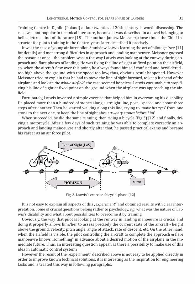
Fortunately, Latwis invented a simple exercise that helped him in overcoming his disability.he placed more than a hundred of stones along a straight line, post - spaced one about threesteps after another. then he started walking along this line, trying to ‘move his eyes’ from onestone to the next one, to keep the line of sight about ‘twenty stones before him’.

When succeeded, he did the same running, then riding a bicycle (Fig.3) [12] and finally, dri-ving a motorcycle. after a few days of such training he was able to complete correctly an ap-proach and landing manoeuvre and shortly after that, he passed practical exams and becamehis career as an air force pilot.

Fig. 3. Latwis´s exercise-’bicycle’ phase [12]

It is not easy to explain all aspects of this „experiment” and obtained results with clear inter-pretation. Some of crucial questions belong rather to psychology, e.g. what was the nature of Lat-wis’s disability and what about possibilities to overcome it by training.

obviously, the way that pilot is looking at the runway in landing manoeuvre is crucial anddoing it properly allows him/her to assess precisely the current state of the aircraft - heightabove the ground, velocity, pitch angle, angle of attack, rate of descent, etc. on the other hand,when the airfield is visible, the pilot controlling the aircraft to complete the approach & flaremanoeuvre knows „something” in advance about a desired motion of the airplane in the im-mediate future. thus, an interesting question appear: is there a possibility to make use of thisidea in automatic control system?

however the result of the „experiment” described above is not easy to be applied directly inorder to improve known technical solutions, it is interesting as the inspiration for engineeringtasks and is treated this way in following paragraphs.

LoNgItUDINaL MotIoN CoNtroL For FLarE PhaSE oF LaNDINg

1. FLarE: - aUtoMatIC CoNtroL oF aIrCraFt MotIoN

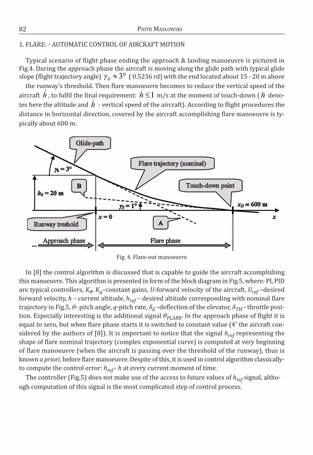
typical scenario of flight phase ending the approach & landing manoeuvre is pictured inFig.4. During the approach phase the aircraft is moving along the glide path with typical glideslope (flight trajectory angle) ( 0.5236 rd) with the end located about 15 - 20 m above

the runway’s threshold. then flare manoeuvre becomes to reduce the vertical speed of the

aircraft , to fulfil the final requirement: m/s at the moment of touch-down ( deno-

tes here the altitude and - vertical speed of the aircraft). according to flight procedures the

distance in horizontal direction, covered by the aircraft accomplishing flare manoeuvre is ty-

pically about 600 m.

Fig. 4. Flare-out manoeuvre

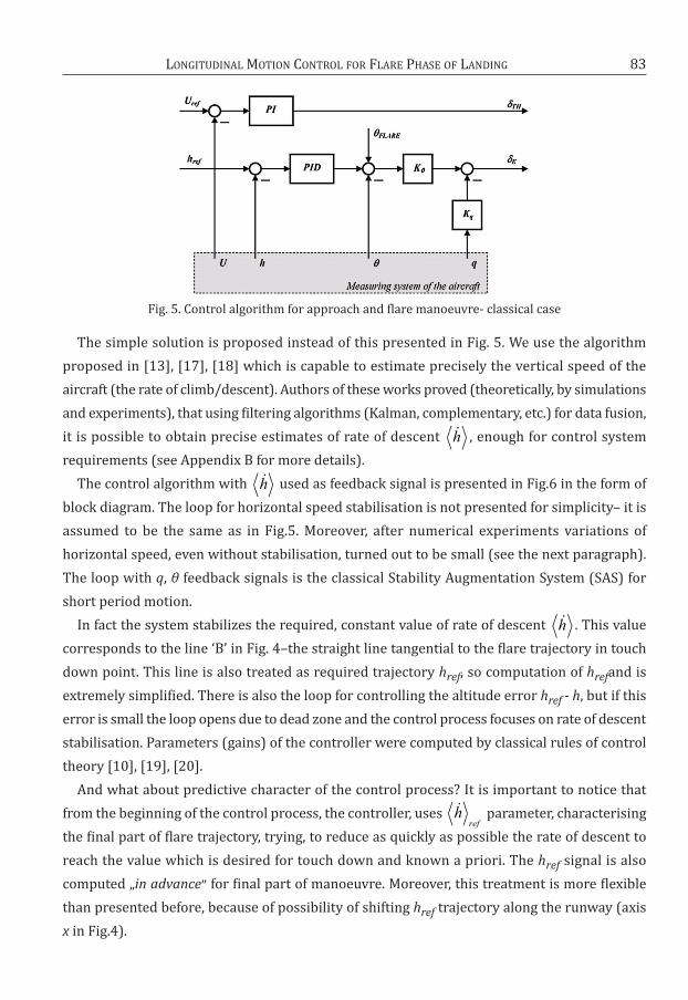
In [8] the control algorithm is discussed that is capable to guide the aircraft accomplishing

this manoeuvre. this algorithm is presented in form of the block diagram in Fig.5, where: PI, PID

are typical controllers, Kθ, Kq–constant gains, U-forward velocity of the aircraft, Uref –desired

forward velocity, h – current altitude, href – desired altitude corresponding with nominal flare

trajectory in Fig.5, θ- pitch angle, q-pitch rate, δE –deflection of the elevator, δTH – throttle posi-

tion. Especially interesting is the additional signal θFLARE. In the approach phase of flight it is

equal to zero, but when flare phase starts it is switched to constant value (4˚ the aircraft con-

sidered by the authors of [8]). It is important to notice that the signal href representing the

shape of flare nominal trajectory (complex exponential curve) is computed at very beginning

of flare manoeuvre (when the aircraft is passing over the threshold of the runway), thus is

known a priori, before flare manoeuvre. Despite of this, it is used in control algorithm classically-

to compute the control error: href - h at every current moment of time.

the controller (Fig.5) does not make use of the access to future values of href signal, altho-

ugh computation of this signal is the most complicated step of control process.

82 PIotr MaSłoWSkI

83

Fig. 5. Control algorithm for approach and flare manoeuvre- classical case

the simple solution is proposed instead of this presented in Fig. 5. We use the algorithm

proposed in [13], [17], [18] which is capable to estimate precisely the vertical speed of the

aircraft (the rate of climb/descent). authors of these works proved (theoretically, by simulations

and experiments), that using filtering algorithms (kalman, complementary, etc.) for data fusion,

it is possible to obtain precise estimates of rate of descent , enough for control system

requirements (see appendix B for more details).

the control algorithm with used as feedback signal is presented in Fig.6 in the form of

block diagram. the loop for horizontal speed stabilisation is not presented for simplicity– it is

assumed to be the same as in Fig.5. Moreover, after numerical experiments variations of

horizontal speed, even without stabilisation, turned out to be small (see the next paragraph).

the loop with q, θ feedback signals is the classical Stability augmentation System (SaS) for

short period motion.

In fact the system stabilizes the required, constant value of rate of descent . this value

corresponds to the line ‘B’ in Fig. 4–the straight line tangential to the flare trajectory in touch

down point. this line is also treated as required trajectory href, so computation of hrefand is

extremely simplified. there is also the loop for controlling the altitude error href - h, but if this

error is small the loop opens due to dead zone and the control process focuses on rate of descent

stabilisation. Parameters (gains) of the controller were computed by classical rules of control

theory [10], [19], [20].

and what about predictive character of the control process? It is important to notice that

from the beginning of the control process, the controller, uses parameter, characterising

the final part of flare trajectory, trying, to reduce as quickly as possible the rate of descent to

reach the value which is desired for touch down and known a priori. the href signal is also

computed „in advance” for final part of manoeuvre. Moreover, this treatment is more flexible

than presented before, because of possibility of shifting href trajectory along the runway (axis

x in Fig.4).

h

h

h

href

LoNgItUDINaL MotIoN CoNtroL For FLarE PhaSE oF LaNDINg

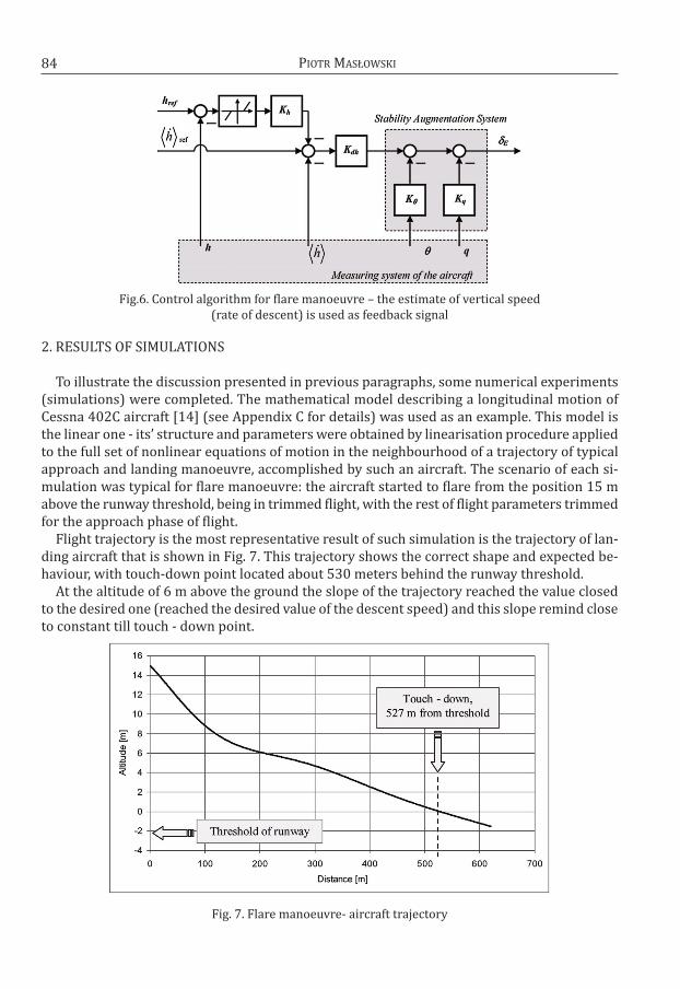
Fig.6. Control algorithm for flare manoeuvre – the estimate of vertical speed (rate of descent) is used as feedback signal

2. rESULtS oF SIMULatIoNS

to illustrate the discussion presented in previous paragraphs, some numerical experiments(simulations) were completed. the mathematical model describing a longitudinal motion ofCessna 402C aircraft [14] (see appendix C for details) was used as an example. this model isthe linear one - its’ structure and parameters were obtained by linearisation procedure appliedto the full set of nonlinear equations of motion in the neighbourhood of a trajectory of typicalapproach and landing manoeuvre, accomplished by such an aircraft. the scenario of each si-mulation was typical for flare manoeuvre: the aircraft started to flare from the position 15 mabove the runway threshold, being in trimmed flight, with the rest of flight parameters trimmedfor the approach phase of flight.

Flight trajectory is the most representative result of such simulation is the trajectory of lan-ding aircraft that is shown in Fig. 7. this trajectory shows the correct shape and expected be-haviour, with touch-down point located about 530 meters behind the runway threshold.

at the altitude of 6 m above the ground the slope of the trajectory reached the value closedto the desired one (reached the desired value of the descent speed) and this slope remind closeto constant till touch - down point.

Fig. 7. Flare manoeuvre- aircraft trajectory

84 PIotr MaSłoWSkI

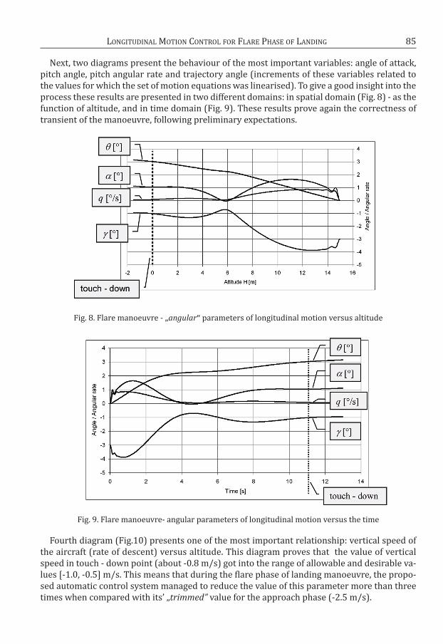
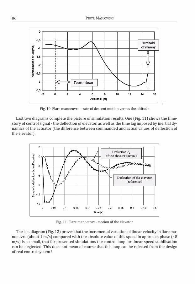
Next, two diagrams present the behaviour of the most important variables: angle of attack,pitch angle, pitch angular rate and trajectory angle (increments of these variables related tothe values for which the set of motion equations was linearised). to give a good insight into theprocess these results are presented in two different domains: in spatial domain (Fig. 8) - as thefunction of altitude, and in time domain (Fig. 9). these results prove again the correctness oftransient of the manoeuvre, following preliminary expectations.

Fig. 8. Flare manoeuvre - „angular” parameters of longitudinal motion versus altitude

Fig. 9. Flare manoeuvre- angular parameters of longitudinal motion versus the time

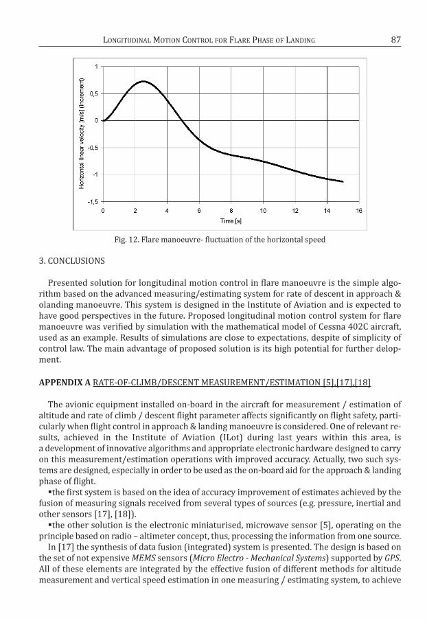
Fourth diagram (Fig.10) presents one of the most important relationship: vertical speed ofthe aircraft (rate of descent) versus altitude. this diagram proves that the value of verticalspeed in touch - down point (about -0.8 m/s) got into the range of allowable and desirable va-lues [-1.0, -0.5] m/s. this means that during the flare phase of landing manoeuvre, the propo-sed automatic control system managed to reduce the value of this parameter more than threetimes when compared with its’ „trimmed” value for the approach phase (-2.5 m/s).

85LoNgItUDINaL MotIoN CoNtroL For FLarE PhaSE oF LaNDINg

F

Fig. 10. Flare manoeuvre – rate of descent motion versus the altitude

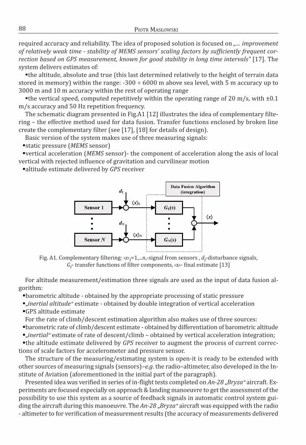
Last two diagrams complete the picture of simulation results. one (Fig. 11) shows the time-story of control signal - the deflection of elevator, as well as the time lag imposed by inertial dy-namics of the actuator (the difference between commanded and actual values of deflection ofthe elevator).

Fig. 11. Flare manoeuvre- motion of the elevator

the last diagram (Fig. 12) proves that the incremental variation of linear velocity in flare ma-noeuvre (about 1 m/s) compared with the absolute value of this speed in approach phase (48m/s) is so small, that for presented simulations the control loop for linear speed stabilisationcan be neglected. this does not mean of course that this loop can be rejected from the designof real control system !

86 PIotr MaSłoWSkI

87

Fig. 12. Flare manoeuvre- fluctuation of the horizontal speed

3. CoNCLUSIoNS

Presented solution for longitudinal motion control in flare manoeuvre is the simple algo-rithm based on the advanced measuring/estimating system for rate of descent in approach &olanding manoeuvre. this system is designed in the Institute of aviation and is expected tohave good perspectives in the future. Proposed longitudinal motion control system for flaremanoeuvre was verified by simulation with the mathematical model of Cessna 402C aircraft,used as an example. results of simulations are close to expectations, despite of simplicity ofcontrol law. the main advantage of proposed solution is its high potential for further delop-ment.

APPENDIx A ratE-oF-CLIMB/DESCENt MEaSUrEMENt/EStIMatIoN [5],[17],[18]

the avionic equipment installed on-board in the aircraft for measurement / estimation ofaltitude and rate of climb / descent flight parameter affects significantly on flight safety, parti-cularly when flight control in approach & landing manoeuvre is considered. one of relevant re-sults, achieved in the Institute of aviation (ILot) during last years within this area, isa development of innovative algorithms and appropriate electronic hardware designed to carryon this measurement/estimation operations with improved accuracy. actually, two such sys-tems are designed, especially in order to be used as the on-board aid for the approach & landingphase of flight. the first system is based on the idea of accuracy improvement of estimates achieved by the

fusion of measuring signals received from several types of sources (e.g. pressure, inertial andother sensors [17], [18]). the other solution is the electronic miniaturised, microwave sensor [5], operating on the

principle based on radio – altimeter concept, thus, processing the information from one source. In [17] the synthesis of data fusion (integrated) system is presented. the design is based on

the set of not expensive MEMS sensors (Micro Electro - Mechanical Systems) supported by GPS.all of these elements are integrated by the effective fusion of different methods for altitudemeasurement and vertical speed estimation in one measuring / estimating system, to achieve

LoNgItUDINaL MotIoN CoNtroL For FLarE PhaSE oF LaNDINg

required accuracy and reliability. the idea of proposed solution is focused on „… improvement

of relatively weak time - stability of MEMS sensors’ scaling factors by sufficiently frequent cor-

rection based on GPS measurement, known for good stability in long time intervals” [17]. thesystem delivers estimates of: the altitude, absolute and true (this last determined relatively to the height of terrain data

stored in memory) within the range: -300 ÷ 6000 m above sea level, with 5 m accuracy up to3000 m and 10 m accuracy within the rest of operating rangethe vertical speed, computed repetitively within the operating range of 20 m/s, with ±0.1

m/s accuracy and 50 hz repetition frequency. the schematic diagram presented in Fig.a1 [12] illustrates the idea of complementary filte-

ring – the effective method used for data fusion. transfer functions enclosed by broken linecreate the complementary filter (see [17], [18] for details of design).

Basic version of the system makes use of three measuring signals:static pressure (MEMS sensor)vertical acceleration (MEMS sensor)- the component of acceleration along the axis of local

vertical with rejected influence of gravitation and curvilinear motionaltitude estimate delivered by GPS receiver

Fig. a1. Complementary filtering: ‹x›i=1,...n,-signal from sensors , di-disturbance signals, Gi- transfer functions of filter components, ‹x›- final estimate [13]

For altitude measurement/estimation three signals are used as the input of data fusion al-gorithm:barometric altitude - obtained by the appropriate processing of static pressure„inertial altitude” estimate - obtained by double integration of vertical accelerationgPS altitude estimateFor the rate of climb/descent estimation algorithm also makes use of three sources:barometric rate of climb/descent estimate - obtained by differentiation of barometric altitude„inertial” estimate of rate of descent/climb – obtained by vertical acceleration integration;the altitude estimate delivered by GPS receiver to augment the process of current correc-

tions of scale factors for accelerometer and pressure sensor.the structure of the measuring/estimating system is open-it is ready to be extended with

other sources of measuring signals (sensors)–e.g. the radio–altimeter, also developed in the In-stitute of aviation (aforementioned in the initial part of the paragraph).

Presented idea was verified in series of in-flight tests completed on An-28 „Bryza” aircraft. Ex-periments are focused especially on approach & landing manoeuvre to get the assessment of thepossibility to use this system as a source of feedback signals in automatic control system gui-ding the aircraft during this manoeuvre. the An-28 „Bryza” aircraft was equipped with the radio- altimeter to for verification of measurement results (the accuracy of measurements delivered

88 PIotr MaSłoWSkI

by this instrument was not worse than 0.9 m within the range of low altitudes). Vertical speedestimates, obtained by data fusion are compared with the result of off – line differentiation ofradio – altitude. Maximum value of discrepancy between these two signals was less than 0.1m/s, thus, taking into account the declared accuracy of radio - altimeter, the accuracy of verti-cal speed estimate obtained by data fusion was assessed to be not worse than 0.05 m/s. thisresult proves that the system works correctly.

results of in-flight tests proved that it is possible to fulfil aforementioned requirements. Mea-suring system, based on fusion of measuring signals obtained from gPS system, vertical acce-lerometers and static pressure sensor, turned out to be capable to compute precise estimate ofvertical speed (with estimated accuracy about 0.05 m/s) as well as the estimate of altitude(with accuracy better than 1 m in discussed case,). additionally it is worth a notice that: in case of gPS signal fade the system continues to work and both vertical speed and alti-

tude estimates are computed continuously, however measuring accuracy decreasessatisfying accuracy and reliability of MEMS sensors and gPS receivers makes this system

applicable also for small and low cost aircraft of general aviation categoryit is possible to extend the proposed structure by including other measuring sub-systems

(e.g. Doppler radio – altimeter or ultrasonic altimeter) in the process of data fusion, to increasethe accuracy and reliability of the whole systemoverall dimensions are small enough for UaV applications.

APPENDIx B: PrEDICtIVE CoNtroL – thE CLaSSICaL aPProaCh

It is convenient to consider a discrete time domain for discussing the idea of automatic con-trol with anticipated behaviour of controlled object. So, we assume that time instants (sam-ples) are denoted by natural numbers: 0, 1, …, k, k+1, and all increments of time from one sampleto the next one are equal i.e.: tk+1-tk=∆t=const for every k. the most typical idea of predictivecontrol algorithm is then based on two general assumptions:

assumption 1: Mathematical model (B1) of a controlled system is known, with y, u denotingrespectively output and control signals (in general, vectors of appropriate dimensions) and G-a causal operator. this model is capable can be used for predicting by computation future be-haviour of controlled object when the future sequence of control signal samples is known.

(B1)

assumption 2: at every current moment of time a reference trajectory y(ref), representing

a desired value of output signal, is known over a finite set of future time instants, called the

prediction horizon. this means that at the moment k values: are known

and L is the prediction horizon.then, control signal applied to the controlled object is computed by optimisation of quadra-

tic quality index:

(B2)

where Q, R are symmetric, positive - definite weighting matrices of appropriate dimensions,

is a series of control signal candidate future samples, while

is a series of predicted output signal samples.

89LoNgItUDINaL MotIoN CoNtroL For FLarE PhaSE oF LaNDINg

90

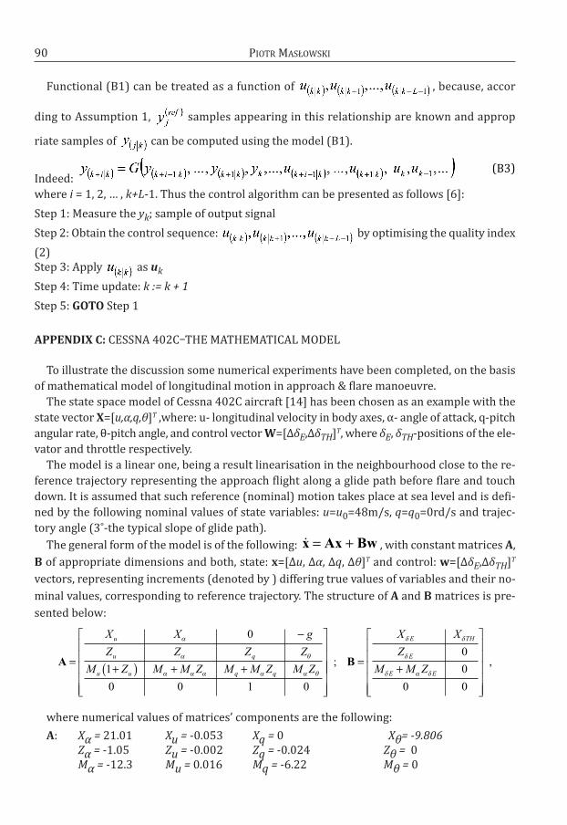
Functional (B1) can be treated as a function of , because, accor

ding to assumption 1, samples appearing in this relationship are known and approp

riate samples of can be computed using the model (B1).

Indeed: (B3)

where i = 1, 2, … , k+L-1. thus the control algorithm can be presented as follows [6]:

Step 1: Measure the yk; sample of output signal

Step 2: obtain the control sequence: by optimising the quality index

(2)Step 3: apply as uk

Step 4: time update: k := k + 1

Step 5: GOTO Step 1

APPENDIx C: CESSNa 402C–thE MathEMatICaL MoDEL

to illustrate the discussion some numerical experiments have been completed, on the basis

of mathematical model of longitudinal motion in approach & flare manoeuvre.

the state space model of Cessna 402C aircraft [14] has been chosen as an example with the

state vector x=[u,α,q,θ]T ,where: u- longitudinal velocity in body axes, α- angle of attack, q-pitch

angular rate, θ-pitch angle, and control vector W=[∆δE,∆δTH]T, where δE, δTH-positions of the ele-

vator and throttle respectively.

the model is a linear one, being a result linearisation in the neighbourhood close to the re-

ference trajectory representing the approach flight along a glide path before flare and touch

down. It is assumed that such reference (nominal) motion takes place at sea level and is defi-

ned by the following nominal values of state variables: u=u0=48m/s, q=q0=0rd/s and trajec-

tory angle (3˚-the typical slope of glide path).

the general form of the model is of the following: , with constant matrices A,

B of appropriate dimensions and both, state: x=[∆u, ∆α, ∆q, ∆θ]T and control: w=[∆δE,∆δTH]T

vectors, representing increments (denoted by ) differing true values of variables and their no-

minal values, corresponding to reference trajectory. the structure of A and B matrices is pre-

sented below:

where numerical values of matrices’ components are the following:

A: Xα = 21.01 Xu = -0.053 Xq = 0 Xθ= -9.806

Zα = -1.05 Zu = -0.002 Zq = -0.024 Zθ = 0Mα = -12.3 Mu = 0.016 Mq = -6.22 Mθ = 0

x Ax Bw= +

A =

−

+( ) + +

X X g

Z Z Z Z

M Z M M Z M M Z M Z

u

u q

u u q q

0

1

0 0 1 0

= +

; ,B

X X

Z

M M Z

E TH

E

E E

0

0

0 0

PIotr MaSłoWSkI

91

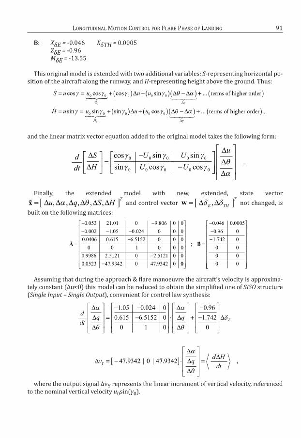
B: XδE = -0.046 XδTH = 0.0005ZδE = -0.96MδE = -13.55

this original model is extended with two additional variables: S-representing horizontal po-sition of the aircraft along the runway, and H-representing height above the ground. thus:

and the linear matrix vector equation added to the original model takes the following form:

Finally, the extended model with new, extended, state vector

and control vector not changed, is

built on the following matrices:

assuming that during the approach & flare manoeuvre the aircraft’s velocity is approxima-tely constant (Δu≈0) this model can be reduced to obtain the simplified one of SISO structure(Single Input – Single Output), convenient for control law synthesis:

where the output signal ΔvY represents the linear increment of vertical velocity, referencedto the nominal vertical velocity u0sin(γ0).

S u u u u

S

= = + ( ) − ( ) −( )cos cos cos sin

0 0 0 0 0

0

∆ ∆ ∆∆

++ ( )

= = + (

...

sin sin sin

terms of higher order

H u u

H

0 0 0

0

)) + ( ) −( ) + ( )∆ ∆ ∆∆

u u0 0cos ... ,

terms of higher order

d

dt

S

H

U U

U U

∆∆

=

−−

cos sin sin

sin cos cos

0 0 0 0 0

0 0 0 0 0

∆∆∆

u

.

w = [ ]∆ ∆ E TH

T,x = [ ]∆ ∆ ∆ ∆ ∆ ∆u q S H

T, , , , ,

A =

− −− − −

−

0 053 21 01 0 9 806 0 0

0 002 1 05 0 024 0 0 0

0 0406 0 615 6 5

. . .

. . .

. . . 1152 0 0 0

0 0 1 0 0 0

0 9986 2 5121 0 2 5121 0 0

0 0523 47 9342 0 47 9342 0

. . .

. . .

−− 00

0 046 0 0005

0 96 0

1 742 0

0 0

0 0

0 0

=

−−−

;

. .

.

.B

d

dtq

∆∆∆

=− −

−

1 05 0 024 0

0 615 6 5152 0

0 1 0

. .

. . ⋅⋅

+−−

= −

∆∆∆

∆

∆

q

v

E

Y

0 96

1 742

0

47 9342 0 4

.

.

. 77 9342. ,[ ]⋅

=∆∆∆

∆

qd H

dt

LoNgItUDINaL MotIoN CoNtroL For FLarE PhaSE oF LaNDINg

92

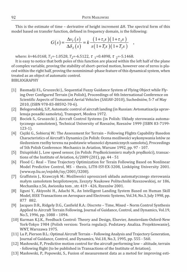
this is the estimate of time – derivative of height increment Δh. the spectral form of thismodel based on transfer function, defined in frequency domain, is the following:

where: k=46.0168, T1=-1.0528, T2=-6.5122, 1=0.4898, 2=-5.1468. It is easy to notice that both poles of this function are placed within the left half of the plane

of complex variable, proving the stability of short–period motion, however one of zeros is pla-ced within the right half, proving the nonminimal–phase feature of this dynamical system, whentreated as an object of automatic control. BIBLIograPhY

[1] Basmadji F.L, gruszecki J., Sequential Fuzzy guidance System of Flying object while Fly-ing over Configured terrain (in Polish), Proceedings of 4th International Conference onScientific aspects of Unmanned aerial Vehicles (SaUaV-2010), Suchedniów, 5-7 of May2010, (ISBN 978-83-88592-70-6).

[2] Belogorodskij, S.P., automatic control of aircraft landing (in russian: avtomatizacija uprav-lenuja posadki samoleta), transport, Moskva 1972.

[3] Bociek S., gruszecki J. aircraft Control Systems (in Polish: Układy sterowania automa-tycznego samolotem), technical University of rzeszów, rzeszów 1999 (ISBN 83-7199-123-1).

[4] Ciężki g., Sobieraj W.: the assessment for terrain – Following Flights Capability BasedonCharacteristics of aircraft’s Dynamics (in Polish: ocena możliwości wykonywania lotów ześledzeniem rzeźby terenu na podstawie własności dynamicznych samolotu), Proceedingsof 5th Polish Conference: Mechanics in aviation, Warsaw 1992, pp. 97 - 107.

[5] Dziupiński J., Low speed sensor, (in Polish: Prędkościomierz małych prędkości), transac-tions of the Institute of aviation, 6/2009 (201), pp. 44 - 51

[6] Flood C.: real – time trajectory optimization for terain Following Based on NonlinearModel Predictive Control, MS – thesis, Lith-ISY-EX-3208, Linköping University 2001.(www.ep.liu.se/exjobb/isy/2001/3208).

[7] graffstein J., krawczyk M.: Możliwości uproszczeń układu automatycznego sterowaniamałym samolotem bezpilotowym, Zeszyty Naukowe Politechniki rzeszowskiej, nr 186,Mechanika z.56, awionika tom , str. 419 - 426, rzeszów 2001.

[8] Iiguni Y., akiyoshi h., adachi N., an Intelligent Landing System Based on human SkillModel, IEEE transactions on aerospace and Electronic Systems, Vol.34, No.3, July 1998, pp.877 882.

[9] Jacques D.r., ridgely D.g., Canfield r.a.: Discrete – time, Mixed – Norm Control Synthesisapplied to aircraft terrain Following, Journal of guidance, Control, and Dynamics, Vol.19,No.5, 1996, pp. 1088 – 1094.

[10] kurman k.J.k., Feedback Control: theory and Design, Elsevier, amsterdam-oxford-NewYork-tokyo 1984 (Polish version: teoria regulacji. Podstawy. analiza. Projektowanie),WNt, Warszawa 1975.

[11] Lu P., Pierson B.L.: optimal aircraft terrain – Following analysis and trajectory generation,Journal of guidance, Control, and Dynamics, Vol.18, No.3, 1995, pp. 555 - 560.

[12] Masłowski, P., Predictive motion control for the aircraft performing low – altitude, terrain- following flight (to be published in transactions of the Institute of aviation).

[13] Masłowski, P., Popowski, S., Fusion of measurement data as a metod for improving esti-

G sv s

sk

s s

s T s T s

Y

E

( ) = ( )( )

=+( ) +( )+( ) +( )

∆∆

1 1

1 1

1 2

1 2

,

PIotr MaSłoWSkI

93

mation quality (in Polish), 1st Congress of Polish Mechanics, Warsaw, august 28 - 31, 2007.[14] McLean D., Zouaoui Z.: an airborne windshear detection system, the aeronautical Journal,

Vol.101, No.1010, Dec. 1997, pp. 447 - 456. [15] Meissner J., the Pilot of Starlit Cognizance (in Polish), Iskry, Warszawa 1970. [16] Nettleton J., Barr D., Schilling B., Lei J., goldwasser S.M.: Micro – Laser range Finder Deve-

lopment: Using the Monolithic approach, report: US arMY CECoM rDEC NVESD, Fort Bel-voir & Bala - Cynwyd, 1999 (www.repairfaq.org/sam/lr/).

[17] Popowski, S., Dąbrowski, W., an integrated measurement of altitude and vertical speed fo-unmanned aerial vehicles, Scientific Proceedings of riga technical University, Series 6:transport and Engineering, pp. 197 – 205, rtU, riga 2008. (ISSN 1407-8015).

[18] Popowski S., Dąbrowski W., Measurement of aircraft’s vertical velocity in landing mano-euvre (in Polish: Pomiar prędkości pionowej samolotu podczas lądowania), Proceedingsof the 5th Conference: avionics, rzeszów, September 2007.

[19] Pułaczewski J., Szacka k., Manitius a., Principles of automatics (in Polish: Zasady auto-matyki), WNt, Warszawa1974.

[20] takahashi Y., rabins ., auslander ., Sterowanie i systemy dynamiczne, WNt Warszawa.[21] timmins W.: operations guide F-16C/D Block 50/52: LaNtIrN aN/aaQ-13 Navigation

Pod, aN/aaQ-14 targeting Pod. (www.freebirdswing.org/tacreference/refMaterial.asp)

PIotr MaSłoWSkI

STEROWANIE RUCHEM PODŁUŻNYM W FAZIE WYRÓWNANIAPODCZAS LĄDOWANIA

Streszczenie

Dyskusja przedstawiona w artykule koncentruje się wokół wybranych zagadnień syntezypraw sterowania automatycznego ruchem podłużnym lądującego samolotu, podczas manewruwyrównania poprzedzającego moment przyziemienia. omówiono niektóre ogólne aspekty pro-cesu sterowania w takim przypadku, aby ujawnić jego predykcyjny charakter. Dyskusja nowychrozwiązań, rozwijanych w Instytucie Lotnictwa dla urządzeń pokładowych przeznaczonych dopomiaru/estymacji prędkości opadania/wznoszenia podczas wykonywania takiego manewru,podkreśla ich efektywność i „nową jakość’ wprowadzaną przez nie do procesu sterowania. roz-ważania ilustruje kilka wyników obliczeń symulacyjnych, wykonanych dla modelu matema-tycznego samolotu Cessna 402C, który został wykorzystany jako przykład. Wyniki tepotwierdzają poprawne działanie proponowanych rozwiązań i ich duży potencjał dla przy-szłych badań.

LoNgItUDINaL MotIoN CoNtroL For FLarE PhaSE oF LaNDINg