looking upstream from breitenbush - usgs · looking upstream from breitenbush station during high...

Looking upstream from Breitenbush station during high flow.

Front cover photograph:

North Santiam River looking downstream from station cableway just upstream from Detroit Lake.

U.S. Department of the InteriorU.S. Geological Survey

Monitoring Instream Turbidity to Estimate Continuous Suspended-Sediment Loads and Yields and Clay-Water Volumes in the Upper North Santiam River Basin, Oregon, 1998–2000

By MARK A. UHRICH and HEATHER M. BRAGG

Water-Resources Investigations Report 03–4098

Prepared in cooperation with The City of Salem

Portland, Oregon: 2003

____________________________________________________________________________

U.S. DEPARTMENT OF THE INTERIOR GALE A. NORTON, Secretary

U.S. GEOLOGICAL SURVEYCHARLES G. GROAT, Director

The use of trade, product, or firm names in this publication is for descriptive purposes only and does not imply endorsement by the U.S. Government.

For additional information: Copies of this report may be purchased from:

District Chief U.S. Geological Survey USGS Information Services 10615 S.E. Cherry Blossom Dr. Box 25286, Federal Center Portland, OR 97216-3159 Denver, CO 80225-0286 E-mail: [email protected] Telephone: 1-888-ASK-USGS Internet: http://oregon.usgs.gov

Suggested citation: Uhrich, M.A., Bragg, H.M., 2003, Monitoring instream turbidity to estimate continuous suspended-sediment loads and yields and clay-water volumes in the Upper North Santiam River Basin, Oregon, 1998–2000: U.S. Geological Survey Water-Resources Investigations Report 03–4098, 43 p.

ii

CONTENTSAcknowledgments ...................................................................................................................................................................... vAbstract ..................................................................................................................................................................................... 1Introduction ............................................................................................................................................................................... 2

Background ........................................................................................................................................................................ 2Purpose and Scope ............................................................................................................................................................. 5

Description of Study Area ......................................................................................................................................................... 5Geography and Geology .................................................................................................................................................... 5Clay Mineralogy ................................................................................................................................................................ 6Land Cover, Land Use, and Vegetation ............................................................................................................................. 8Climate and Precipitation................................................................................................................................................... 8Hydrology and Channel Geomorphology ........................................................................................................................ 10

Overview of Turbidity and Suspended Sediment ................................................................................................................... 11Turbidity Regulations ...................................................................................................................................................... 11Measurement of Turbidity .............................................................................................................................................. 11Turbidity and Stream Discharge ...................................................................................................................................... 12Turbidity and Suspended-Sediment ................................................................................................................................. 12Erosion and Suspended Sediment .................................................................................................................................... 12

Methods of Investigation......................................................................................................................................................... 13Monitoring Network ........................................................................................................................................................ 13

Historic Gaging Stations ..................................................................................................................................... 13Active Water-Quality Stations ............................................................................................................................ 13

Data Collection ................................................................................................................................................................. 15Site instrumentation.............................................................................................................................................. 15Streamflow and Water-Quality Data Collection .................................................................................................. 15Suspended-Sediment Sampling............................................................................................................................ 15Persistent-Turbidity Sampling and Processing .................................................................................................... 18Detroit Lake Persistent-Turbidity Sampling ........................................................................................................ 20

Quality Assurance ............................................................................................................................................................. 20Data Collection..................................................................................................................................................... 20Instrument Calibration.......................................................................................................................................... 22

Data Calculations .............................................................................................................................................................. 22Suspended-Sediment Load Calculations.............................................................................................................. 22Persistent-Turbidity Calculations ......................................................................................................................... 24Clay-Water Volume Calculations ........................................................................................................................ 24

Results ..................................................................................................................................................................................... 25Estimated Annual Suspended-Sediment Loads ................................................................................................................ 25Estimated Annual Suspended-Sediment Yields................................................................................................................ 28Sand-Silt Partition Analysis .............................................................................................................................................. 28Persistent Turbidity Analysis ............................................................................................................................................ 30

Turbidity-Decay Curves for the Annual Peak Streamflow Events ...................................................................... 30Analysis of Stream Persistent Turbidity............................................................................................................... 35Turbidity-Decay Curves for Detroit Lake ............................................................................................................ 35

Clay-Water Volume Analysis ........................................................................................................................................... 35Annual Clay-Water Volumes ............................................................................................................................... 36Annual Clay-Water Yields ................................................................................................................................... 36

Future Studies........................................................................................................................................................................... 38Summary ................................................................................................................................................................................. 38References Cited ...................................................................................................................................................................... 40

iii

FIGURES

Figure 1. Map showing location of data collection sites in the North Santiam River Basin .................................................... 3Figure 2. Map showing surficial geology of the North Santiam River Basin .......................................................................... 7Figure 3. Map showing land cover in the North Santiam River Basin.............................................................................................. 9Figure 4. Graphs showing discharge at time of sample collection in water years 1999 and 2000 at three monitoring

sites in the upper North Santiam River Basin ........................................................................................................ 17Figure 5. Graph showing streamflow duration curves and discharge at time of sample collection in water years 1999

and 2000 at three monitoring sites in the upper North Santiam River Basin......................................................... 18Figure 6. Graph showing turbidity decay curve for sample collected December 29, 1998, at Blowout Creek sampling

station ................................................................................................................................................................... 20Figure 7. Diagram showing theoretical fall distances at 4 degrees Celsius for different fine-particle sizes at selected

time intervals in Detroit Lake reservoir, Oregon ................................................................................................... 21Figure 8. Graphs showing relation of turbidity and discharge to suspended-sediment concentrations at three monitoring

sites in the upper North Santiam River Basin ........................................................................................................ 23Figure 9. Graph showing relation of persistent turbidity to initial turbidity at three monitoring sites in the upper

North Santiam River Basin in water years 1999 and 2000 .................................................................................... 25Figure 10. Graphs showing relation of sampled suspended-sediment concentrations (using uncorrected and bias-

corrected regressions) to turbidity at three monitoring sites in the upper North Santiam River Basin, water years 1999 and 2000..................................................................................................................................... 27

Figure 11. Graph showing estimated annual and peak storm suspended-sediment loads at three monitoring sites inthe upper North Santiam River Basin, water years 1999 and 2000 ....................................................................... 28

Figure 12. Graphs showing continuous turbidity data from three monitoring sites in the upper North Santiam River Basinfor the peak storms of water years 1999 and 2000................................................................................................ 29

Figure 13. Graph showing relation of measured to estimated suspended-sediment concentrations at three monitoring sites in the upper North Santiam River Basin, water years 1999 and 2000 ........................................................... 30

Figure 14. Graphs showing relation of measured to estimated suspended-sediment loads at three monitoring sites in theupper North Santiam River Basin, water years 1999 and 2000 ............................................................................. 31

Figure 15. graph showing statistical distribution of estimated mean daily suspended-sediment loads at three monitoring sites in the upper North Santiam River Basin, water years 1999 and 2000 ........................................................... 32

Figure 16. Graph showing estimated annual suspended-sediment yields at three monitoring sites in the upper North Santiam River Basin, water years 1999 and 2000 ....................................................................................... 32

Figure 17. Graphs showing relation of suspended-sediment concentration to percent fine material in samples fromthree monitoring sites in the upper North Santiam River Basin, water years 1999 and 2000 ............................... 33

Figure 18. Graphs showing turbidity decay curves for samples collected during the peak storms of water years 1999 and 2000 at three monitoring sites in the upper North Santiam River Basin......................................................... 34

Figure 19. Graphs showing statistical distribution of persistent-turbidity values at three monitoring sites in the upper North Santiam River Basin, water years 1999 and 2000 .............................................................................36

Figure 20. Map showing sampling sites on Detroit Lake reservoir, North Santiam River Basin, December 29, 1998........... 36Figure 21. Graphs showing turbidity decay curves for samples collected from Detroit Lake reservoir on December 29,

1998, during the peak storm of water year 1999.................................................................................................... 37Figure 22. Graphs showing estimated annual suspended-clay-water volumes and yields calculated from data collected

at three monitoring sites in the upper North Santiam River Basin, water years 1999 and 2000 ........................... 38

TABLES

Table 1. Turbidity in the North Santiam River Basin, February and March 1996................................................................... 4 Table 2. Percentages of rock types exposed at the surface in the North Santiam River Basin upstream from the

Salem water treatment plant and from sampling sites in three subbasins upstream of Detroit Lake ......................... 8Table 3. Percentages of land cover types in the North Santiam River Basin upstream from the Salem water treatment

plant and from sampling sites in three subbasins upstream from Detroit Lake........................................................ 10Table 4. Streamflow extremes for upper North Santiam River Basin sites, water years 1999 and 2000 .............................. 11Table 5. North Santiam River Basin streamflow and water-quality monitoring network......................................................14Table 6. Starting date for streamflow and water-quality data collection at USGS North Santiam River Basin stations ....... 14Table 7. Fall times for suspended-sediment particles and schedule for aliquot withdrawals ............................................... 20

iv

Table 8. Power regression equations for estimating suspended-sediment concentrations from streamflow data......................................................................................................................................................... 26

Table 9. Power regression equations for estimating suspended-sediment concentrations from instream turbidity-monitor data ...................................................................................................................... 26

Table 10. Peak instantaneous turbidity and estimated instantaneous suspended-sediment load values for water years 1999 and 2000 ....................................................................................................................................... 29

Table 11. Estimated suspended-sediment loads and yields...................................................................................................... 32 Table 12. Log10-transformed, linear regression equations for estimating persistent turbidity from initial

whole-water turbidity................................................................................................................................................ 36 Table 13. Clay-water volumes and yields estimated from data collected at three monitoring sites in the upper

North Santiam River Basin, water years 1999 and 2000.......................................................................................... 39

ACKNOWLEDGMENTS

The authors thank the City of Salem for cooperative funding , and City of Salem employees Libby Barg, Tim Sherman, and Henry Wujcik, for providing valuable technical expertise and field assistance. We also thank David Klug and David Halemeier of the U.S. Forest Service, Detroit Ranger District, for their technical leadership and field assistance. Special thanks to Amy Brooks of the U.S. Geological Survey for her unceasing efforts in the maintenance and calibration of the water-quality probes and for providing the final data. Others within the U.S. Geological Survey who assisted in the collection of samples and who contributed their considerable technical skills include Douglas Cushman, Tom Herrett, Richard Kittelson, Tirian Mink, and Jay Spillum.

v

Monitoring Instream Turbidity to Estimate Continuous Suspended-Sediment Loads and Yields and Clay-Water Volumes in the Upper North Santiam River Basin, Oregon, 1998–2000

By Mark A. Uhrich and Heather M. Bragg

Abstract

Three real-time, instream water-quality and turbidity-monitoring sites were established in October 1998 in the upper North Santiam River Basin on the North Santiam River, the Breitenbush River, and Blowout Creek, the main tributary inputs to Detroit Lake, a large, controlled reservoir that extends from river mile 61 to 70. Suspended-sediment samples were collected biweekly to monthly at each station. Rating curves provided estimated suspended-sediment concentration in 30-minute increments from log-transformations of the instream turbidity monitoring data. Turbidity was found to be a better surrogate than discharge for estimating suspended-sediment concentration. Daily and annual mean suspended-sediment loads were estimated using the estimated suspended-sediment concentrations and corresponding streamflow data.

A laboratory method for estimating persistent (residual) turbidity from separate turbidity samples was developed. Turbidity was measured over time for each sample. Turbidity decay curves were derived as the suspended sediment settled. Each curve was used to estimate a turbidity value for a given settling time. Medium to fine clay particle (< 0.002 mm [millimeter] diameter) settling times of 8.5 hours were computed using Stokes law. An average of 30 persistent-turbidity samples was collected from each of the 3 sites. These samples were used to estimate the 0.002 mm-size clay particle persistent turbidity for each site. The monitored instream 30-minute turbidity values

were converted to a calculated persistent turbidity value that would have resulted after 8.5 hours of settling in the laboratory. Persistent turbidities of 10 NTU (nephelometric turbidity units) and above were tabulated for each site. (Water of 10 NTU and above can interfere with or damage treatment filters and result in intake closures at drinking-water facilities.)

A method was developed that used the persistent-turbidity experiments, turbidity decay curves, and stream discharge to estimate the volume of water containing suspended clay that entered Detroit Lake from the three main tributaries. “Suspended-clay water” was defined as water having a value of at least 10 NTU after settling the required 8.5 hours. The suspended-clay concentrations of 10 NTU or higher were paired with the corresponding stream discharge in the continuous record. These summed discharges represent the annual volume of water containing suspended clay that entered Detroit Lake from the three main tributaries.

Higher yields (load per unit area) of sus-pended sediment and suspended-clay water were observed from the smaller Breitenbush River and Blowout Creek subbasins than from the main-stem North Santiam River for water years 1999 and 2000. The 3-day peak streamflow and turbidity events in 1999 and 2000 carried two- thirds of the annual suspended-sediment load for the three subbasins. Turbidity and suspended- sediment concentration relations within the upper North Santiam River Basin are basin specific and can change annually within a single subbasin.

1

Techniques developed during this study will assist water resource planners in understanding and managing water quality in their watersheds, particularly those in which there are persistent- turbidity problems.

INTRODUCTION

Background

The City of Salem, Oregon, uses the North Santiam River as its primary drinking water source. The North Santiam River drains approximately 690 mi2

upstream from the City of Salem’s water-treatment facility near Stayton (fig. 1). A dam on the North Santiam River created Detroit Lake, a controlled reservoir with 436,000 acre-feet of storage capacity at maximum pool elevation. Big Cliff Reservoir, a smaller reregulating reservoir just below Detroit Lake, with 2,430 acre-feet of usable storage capacity, is used to stabilize water releases from Detroit Dam. Besides providing recreation and flood control, both dams are used for power generation. Detroit Dam, which releases water at 360 feet above the channel bottom, and Big Cliff Dam, which releases at 126 feet above the channel bottom, have 100,000 and 18,000 kilowatt powerhouses, respectively. Neither powerhouse has capabilities for selective withdrawal of water from different lake depths.

The City of Salem’s water-treatment facility, which uses a slow-sand filtration system, supplies water to approximately 170,000 customers in the Salem metropolitan area, which use an average of 30 MGD (million gallons per day); demand sometimes peaks at 60 MGD. The sand and gravel layers of the filter remove inorganic clay and larger particles. Protozoa, algae, and other invertebrates on the filter surface form a biological layer that helps to remove biological and other organic contaminants. By 2020, the Salem area water-service population is projected to grow to 230,000; at peak water demand, including a 10 percent reduction for conservation, this population, along with industrial users, would require approximately 90 MGD (City of Salem, 1999).

Extreme high-flow events and floods occurred throughout Western Oregon and in the North Santiam River Basin during 1996 and 1997, resulting in an increase in turbidity (which is caused by suspended clay, silt, and other particulate matter). Elevated

turbidity persisted for several months and surpassed the ability of the Salem treatment plant to filter the water, subsequently disrupting normal delivery of water to the Salem metropolitan area for about a month. During the February 1996 flood, 8 to 15 inches of precipitation fell on the basin over a 4-day period. In addition, the rain was sufficiently warm to melt the preexisting snowpack. Salem’s water treatment facility was inundated with turbid water and was forced to shut down for 8 days. About 4 million gallons of water per day was acquired from the neighboring City of Keizer and other emergency wells, aquifer storage systems, and municipalities (Cotton et al., 1998; Katherine Willis, City of Salem, written commun., 1996).

Other emergency measures were invoked in February 1996 that included applying pretreatment chemicals to reduce turbidity to 5 NTU (nephelometric turbidity units). In 1997 a pretreatment facility was constructed in order to process highly turbid water and remove the silt and clay particles by applying alum and soda ash; these measures required a significant increase in operating and personnel costs. However, since 1997 and through September 2000, Salem’s water intakes also were closed for approximately nine high-flow, storm-related episodes of less than 48 hours per closure, due to the silt and clay-laden water passing through the treatment system. There were eight episodes where the treatment facility was taken out of service for more than 48 hours and required operation of the pre-treatment facility as turbidity levels increased to over 10 NTU (Timothy Sherman, City of Salem, written commun., 2003).

Ruffing, et al. (1997) described the events in the North Santiam River Basin during and following the February 3–9, 1996 storm: On February 6, turbidity values measured in the North Santiam River at the Salem’s water-supply intake began to rise, peaking first on February 7 at near 100 NTU, as measured by the U.S. Army Corps of Engineers, due principally to water flowing from the Little North Santiam River, a lower-basin tributary near river mile (RM) 39. The February 1996 turbidity measurements were collected only as single daily readings, so instantaneous turbidity peak values could have been higher. A second turbidity peak of near 140 NTU, again recorded by daily readings at the water treatment plant intake, occurred on February 14 due to the delayed response of water released from Detroit and Big Cliff reservoirs after the February 3–9 storm (table 1). By March 10 the turbidity values had declined to 10 NTU at the

2

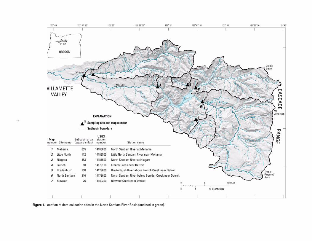
3

Figure 1. Location of data collection sites in the North Santiam River Basin (outlined in green).

s

Table 1. Turbidity in the North Santiam River Basin, February and March 1996 [NTU, nephelometric turbidity units; recorded as single daily readings]

Turbidity Turbidity Turbidity Turbidity Location February 7 February 14–15 February 21 March 10

Salem Water Treatment Plant 100 NTU 140 NTU 10 NTU

Detroit Lake #1 at water surface 55 NTU 30 NTU

Detroit Lake #1 at 170 ft. depth 136 NTU


Detroit Lake #2 at water surface 77 NTU 43 NTU



Big Cliff Reservoir at water surface 213 NTU 112 NTU

North Santiam River at river mile 71 8 to 12 NTU

Little North Santiam River at mouth 21 NTU

treatment plant. (A slow-sand filtration system is unable to treat water with turbidity values higher than 10 NTU.)

The highest observed turbidity values in the North Santiam River Basin during this storm were recorded on February 14–15 at two locations in Detroit Lake, where values ranged from 55 and 77 NTU at the surface to 328 and 389 NTU at depths of 215 and 257 feet, respectively, and at the surface of Big Cliff Reservoir, downstream from Detroit Lake, where the turbidity measured 213 NTU (table 1). In contrast, on February 14–15 at 0.5 miles upstream from Detroit Lake on the North Santiam River near RM 71, turbidity ranged from 8 to 12 NTU, and on the Little North Santiam River near the mouth at Mehama, at RM 39, the turbidity was 21 NTU. On February 21, the two Detroit Lake readings ranged from 30 and 43 NTU at the surface to 136 and 388 NTU at depths of 170 and 290 feet, respectively, and surface readings on Big Cliff Reservoir were 112 NTU. No readings were taken from the tributaries that day.

In order to flush the highly turbid water from Detroit Lake, releases were initially discharged over the dam spillway. These releases continued until February 14, after which the spillway was closed and water was discharged through both the penstock and upper regulating outlet, which were about 145 and 208 feet, respectively, below the water surface on February 14. By February 21 about 46 percent of the volume in Detroit Lake had been flushed, and by February 29 approximately 67 percent of the total 350,000 acre-feet of Detroit Lake volume on February 14 had been released, which dropped the lake level by approximately 33 feet from the February 14 level.

At the time of the February 1996 event, a real-time water quality and turbidity monitoring network had not yet been established in the North Santiam River Basin. Turbidity and other water-quality readings were collected sporadically at only three locations in the basin and represented only single readings in a 24-hour or more period. The main-stem river and tributaries to Detroit Lake may have reached significantly higher levels of turbidity than what was measured. Without continuous, instream-monitoring equipment, it is not possible to determine instantaneous turbidity levels and other water-quality parameters between measurements.

In 1998, the U.S. Geological Survey began a cooperative study with the City of Salem to investigate the sources and dynamics of suspended sediment in the North Santiam River. A real-time streamflow and water-quality monitoring network was installed in the North Santiam River Basin. Continuous streamflow, water temperature, specific conductance, pH, and turbidity data collection began in October 1998 at three sites upstream of Detroit Lake. Three sites were added downstream of Detroit Lake in April 2000, and one additional site upstream of the lake was installed in July 2001. Information derived from the study will help locate sources of suspended sediment within the basin and be used to facilitate the operation of the City of Salem’s water-treatment plant with regard to turbidity and sediment loads entering water intakes, settling ponds, and pretreatment systems. Sediment load information also can be used to estimate reservoir siltation in Detroit Lake, (Sidle and Campbell, 1985; Gippel, 1989; Ewing and Mohrman, 1989). A report by the U.S. Army Corps of Engineers, written soon after

4

the construction of the Detroit Dam and powerhouse, estimated that Detroit Lake would fill with sediment at the rate of 175 acre-feet per year (U.S. Army Corps of Engineers, 1953). The suspended-sediment load estimates from this study could help verify those siltation estimates. Primary tasks of the study included: • Establishing a network of real-time streamflow

and water-quality monitoring stations to record both short- and long-term spatial and temporal conditions, trends in streamflow, and basic water quality parameters (water temperature, specific conductance, pH), as well as turbidity, in the North Santiam River Basin, both upstream and downstream of Detroit Lake.

• Estimating daily and annual suspended-sediment loads for the major subbasins and main-stem North Santiam River, using correlations developed between instream turbidity and suspended-sediment concentrations.

• Identifying the relative short- and long-term contribution of persistent-(residually) turbid water from the major subbasins and other primary sources to Detroit Lake and the North Santiam River upstream of the City of Salem’s water intake.

• Defining the relation between landscape features and watershed characteristics and total and clay-fraction suspended-sediment loads for the subbasins upstream from each monitoring station.

• Establishing an early warning system to monitor high streamflow and turbidity events in the North Santiam River Basin that may affect operation of the City of Salem’s water treatment plant, control of Detroit Lake reservoir, forest road maintenance, and downstream flood management.

Purpose and Scope

The purpose of this report is to describe the network of real-time streamflow and water-quality monitoring stations established in the North Santiam River Basin and present the correlations developed between data from the continuous instream turbidity monitors and from samples collected for suspended-sediment analysis. Also presented are estimates of the annual suspended-sediment loads and yields, and volumes of water containing suspended clay for the three monitoring sites established in 1998 upstream of

Detroit Lake, for the period October 1998 to September 2000.

Real-time streamflow and basic water-quality data, including turbidity, used in this report, were collected, quality-assessed, and processed from October 1998 through September 2000. The suspended-sediment concentration and persistent- turbidity data were collected from October 1998 through September 2001. Suspended-sediment data collection and operation of all water-quality monitoring stations is planned at least through September 2003 for all sites in the network, providing 5 years of data.

DESCRIPTION OF STUDY AREA

Geography and Geology

The North Santiam River Basin is bounded by the Cascade Range to the east and the Willamette Valley to the west (fig. 1). The basin drains west. The eastern boundary extends from Olallie Butte in the north to Three Fingered Jack in the south. Elevations along the 25-mile eastern edge surpass 8,000 feet above sea level, with Mount Jefferson, a glaciated volcanic peak, the highest point at nearly 10,500 feet. Approximately 40 percent of the North Santiam River Basin upstream of the Salem water treatment plant, near Stayton, is 3,000 feet in elevation or higher. Areas upstream of Detroit Lake have steeper terrain and higher elevations than areas downstream of the lake. About three-fifths percent of the major subbasins upstream of Detroit Lake have elevations of 3,000 feet and above.

The North Santiam River Basin upstream of the Salem water treatment plant is in two principle ecoregions (Omernick and Gallant, 1986). The Western Cascades ecoregion forms most of the western slope of the mountain range and comprises 78 percent of the basin, of which 51 percent is considered montane highlands, 24 percent lowlands and valleys with 3 percent subalpine or alpine (U.S. Environmental Protection Agency, 1996). The stratigraphy within this province is an older, deeply dissected sequence of volcanically deformed and partially altered flows and pyroclastic rocks, with some steep terrain (70 percent slopes are common in places) and moderately incised canyons. The Cascade Crest ecoregion, which encom- passes 17 percent of the basin, has younger stratigraphy and forms a wide topographic high with relatively

5

gentle slopes in comparison to the Western Cascades province. The remaining 5 percent of the basin is considered valley foothills. The North Santiam River Basin slopes westerly and is composed of undeformed and unaltered andesitic and basaltic lava flows and cones, highlighted by the prominent stratovolcanos and nearly undissected shield (depending on glacial history) of the Cascade Range. The valley foothills portion is composed mostly of alluvial and Columbia River Basalt deposits.

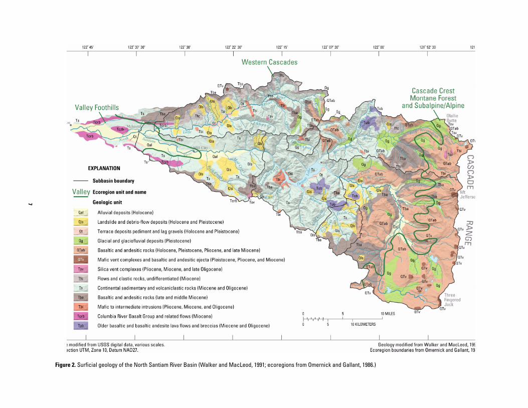
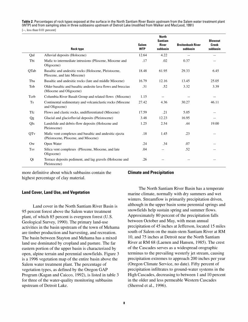
Sixty-two percent of the basin upstream of Stayton is composed of older Tertiary period basalts, which overlay and interfinger with tuffaceous sedimentary rocks and breccia (fig. 2). The middle basin, from the ridge tops above Detroit Lake to near Mehama, is composed primarily of these older Western Cascade volcanics dating from the late Oligocene to late Pliocene. Approximately 38 percent of the basin is younger basalts, alluvium, and glacial deposits of the Quaternary period. The upper basin is dominated by these younger High Cascade basalts, andesites, and landslide deposits of the Pleistocene to the present, with most of the lava and ash ejected within the last million years. Dotted along the margin between the High and Western Cascades provinces are ridge- capping basalt flows of early Pliocene age. The lower basin, below Mehama, is a more recent, large, alluvial plain, except where the volcanic and marine sedimentary rocks of the Pliocene and Miocene age are exposed in the foothills (fig. 2). (The above description was synthesized from Peck et al., 1964; Walker and MacLeod, 1991; and Sherrod et al., 1996.) Table 2 provides percentages of rock types from figure 2 for the entire basin upstream of the Salem water treatment plant and for the three monitored subbasins upstream of Detroit Lake.

Clay Mineralogy

Studies have identified assemblages of colloidal minerals in both the water column and in alluvial fan and delta areas of Western Cascade streams and reservoirs (Youngberg et al., 1971; Ambers, 1998; Glasmann, 1998). Smectite and other amorphous clays, along with poorly formed crystalline materials, are the primary clay minerals within these assemblages responsible for the persistent ambient turbidity in the North Santiam River and other Western Cascade basins (Bates et al., 1998; Pearch, 2000). The older, weathered

basalts and volcaniclastic rocks of the Western Cascades may be responsible for the suspended clay and resulting high persistent turbiditities in Detroit Lake and surrounding streams after storm events. This is particularly true where large, deep-seated earthflow failures intersect stream channels. The younger rocks of the High Cascades are more stable, less hydrothermally altered and erodible, than those of the Western Cascades. Consequently, the less developed clays do not provide as great a source of persistent turbidity-causing material (Taskey, 1978; Bates et al., 1998; Pearch, 2000).

Montmorillonite-group clays, such as smectite, are very small, (less than 0.05–0.08 µm [micrometers] in diameter), electrically charged particles, with marked expansion, absorption, and adsorption properties. These particles will remain suspended in the water column for extended periods and can pass through water treatment filters. Other clay minerals, such as chlorite, kaolinite, and illite, are also present but are larger, more neutrally charged particles that tend to settle out of suspension in less time, although these larger clays form muddy deposits near the reservoir margins and tributary delta areas of Detroit Lake. Resuspension of reservoir sediments by the cyclic filling of reservoirs like Detroit Lake may also contribute to downstream persistent turbidity (Ambers, 1998; Bates et al., 1998).

The Breitenbush River and Blowout Creek subbasins contain predominantly older Miocene and Oligocene, heavily weathered and hydrothermally altered rocks. These aged basalts, andesites, and other volcaniclastic rocks contain more of the residual turbidity-causing materials, such as smectite and halloysite, than the younger rocks of the Holocene, Pleistocene, and Pliocene age present in the upper North Santiam River subbasin, since soils in the other two subbasins have had more time to develop and erode. Other sediment producing units unique to each subbasin include the glacial deposits in the Breitenbush and North Santiam subbasins and the landslide and debris-flow deposits in the Blowout subbasin, although the clay component of each of these is probably less than the older, more developed soils and erodible rocks. Hence, according to figure 2, the Blowout subbasin appears to contain the highest potential clay source, followed by the Breitenbush subbasin, then the North Santiam subbasin, although additional soil and hydrogeologic maps of greater detail are needed to be

6

7

Figure 2. Surficial geology of the North Santiam River Basin (Walker and MacLeod, 1991; ecoregions from Omernick and Gallant, 1986.)

-- --

--

-- -- --

--

--

--

--

-- --

-- -- --

Table 2. Percentages of rock types exposed at the surface in the North Santiam River Basin upstream from the Salem water treatment plant (WTP) and from sampling sites in three subbasins upstream of Detroit Lake (modified from Walker and MacLeod, 1991) [--, less than 0.01 percent]

North Santiam Blowout

Salem River Breitenbush River Creek Rock type WTP subbasin subbasin subbasin

Qal Alluvial deposits (Holocene) 12.64 4.22

Tbi Mafic to intermediate intrusions (Pliocene, Miocene and Oligocene)

.17 .02 0.37

QTab Basaltic and andesitic rocks (Holocene, Pleistocene, Pliocene, and late Miocene)

18.48 61.95 29.33 6.45

Tba Basaltic and andesitic rocks (late and middle Miocene) 16.79 12.16 13.45 25.05

Tob Older basaltic and basaltic andesite lava flows and breccias .31 .52 3.32 3.39 (Miocene and Oligocene)

Tcrb Columbia River Basalt Group and related flows (Miocene) 1.15

Ts Continental sedimentary and volcaniclastic rocks (Miocene and Oligocene)

27.42 4.36 30.27 46.11

Tfc Flows and clastic rocks, undifferentiated (Miocene) 17.59 .21 5.05

Qg Glacial and glaciofluvial deposits (Pleistocene) 3.48 12.23 16.95

Qls Landslide and debris-flow deposits (Holocene and Pleistocene)

1.25 2.54 .44 19.00

QTv Mafic vent complexes and basaltic and andesitic ejecta (Pleistocene, Pliocene, and Miocene)

.18 1.45 .23

Ow Open Water .24 .34 .07

Tsv Silica vent complexes (Pliocene, Miocene, and late Oligocene)

.04 .52

Qt Terrace deposits pediment, and lag gravels (Holocene and Pleistocene)

.26

more definitive about which subbasins contain the highest percentage of clay material.

Land Cover, Land Use, and Vegetation

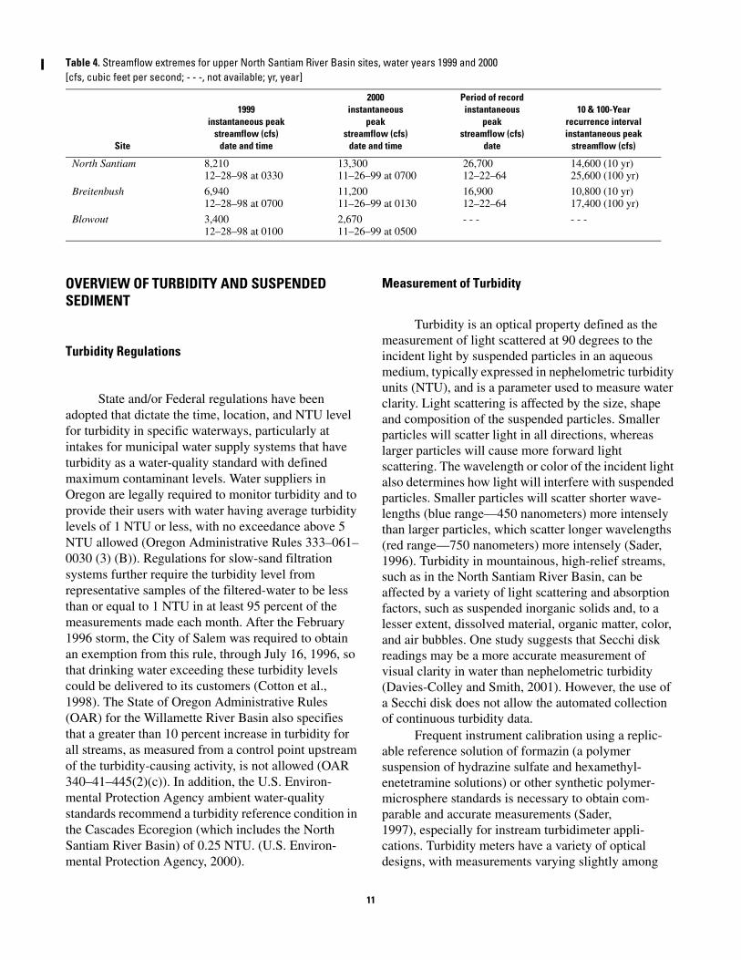
Land cover in the North Santiam River Basin is 95 percent forest above the Salem water treatment plant, of which 85 percent is evergreen forest (U.S. Geological Survey, 1990). The primary land-use activities in the basin upstream of the town of Mehama are timber production and harvesting, and recreation. The basin between Stayton and Mehama has a mixed land use dominated by cropland and pasture. The far eastern portion of the upper basin is characterized by open, alpine terrain and perennial snowfields. Figure 3 is a 1996 vegetation map of the entire basin above the Salem water treatment plant. The percentage of vegetation types, as defined by the Oregon GAP Program (Kagan and Caicco, 1992), is listed in table 3 for three of the water-quality monitoring subbasins upstream of Detroit Lake.

Climate and Precipitation

The North Santiam River Basin has a temperate marine climate, normally with dry summers and wet winters. Streamflow is primarily precipitation driven, although in the upper basin some perennial springs and snowfields help sustain spring and summer flows. Approximately 80 percent of the precipitation falls between October and May, with mean annual precipitation of 45 inches at Jefferson, located 15 miles south of Salem on the main-stem Santiam River at RM 10, and 75 inches at Detroit near the North Santiam River at RM 68 (Laenen and Hansen, 1985). The crest of the Cascades serves as a widespread orographic terminus to the prevailing westerly jet stream, causing precipitation extremes to approach 200 inches per year (Oregon Climate Service, no date). Fifty percent of precipitation infiltrates to ground-water systems in the High Cascades, decreasing to between 1 and 10 percent in the older and less permeable Western Cascades (Sherrod et al., 1996).

8

9

Figure 3. Land cover in the North Santiam River Basin.

--

-- --

--

-- --

-- -- --

-- --

--

-- -- --

Table 3. Percentages of land cover types in the North Santiam River Basin upstream from the Salem water treatment plant (WTP) and from sampling sites in three subbasins upstream from Detroit Lake (source: Kagan and Caicco, 1992). [--, less than 0.01 percent]

Land cover Salem WTP

North Santiam River subbasin

Breitenbush River subbasin

Blowout Creek subbasin

Agricultural cropland and pastureland 10.46 0.00 0.00 0.00

Alpine communities 2.49 6.60 4.35

Douglas fir-Oregon white oak forest and woodland 2.00 .00

Douglas fir-western hemlock-grand fir forest 52.86 39.90 55.60 72.45

Mixed conifer and broadleaf deciduous forest 4.91 6.72 .12 5.24

Mountain hemlock forest 7.57 19.02 13.34

Mountain hemlock parkland .56 1.97

Oak-Douglas fir-ponderosa pine-pasture-urban mosaic .51

Open water .68 .20

Recent timber harvest areas as seen from July 1988 imag- 6.35 6.12 11.33 .64 ery (harvested approximately 1980 to 1988)

Silver fir-western hemlock-noble fir forest 10.65 17.17 14.87 21.67

Subalpine lodgepole pine forest and woodland .71 2.30 .39

Urban and industrial .25

Hydrology and Channel Geomorphology

The mean annual high and low flows at the North Santiam River below Boulder Creek near Detroit gage (North Santiam—USGS station 14178000) are 15,000 and 289 cfs (cubic feet per second), respectively, based on the period 1908–1987. The mean annual high and low flows at the Breitenbush River above French Creek gage (Breitenbush—USGS station 14179000), based on the period 1933–1987, are 10,600 and 88 cfs, respectively (Wellman et al., 1993). The magnitude and probabilities of the high and low flows are computed on an annual basis for a 1-day consecutive period with a 50-year recurrence interval. The respective 7-day low flows for 2- and 10- year recurrence intervals are 391 and 325 cfs for North Santiam, and 123 and 100 cfs for Breitenbush.

The water year 1999 and 2000 annual mean streamflows at North Santiam were 1,334 and 1,111 cfs, respectively, 32 and 10 percent above normal for the 74 years of record. The annual mean streamflow at Breitenbush was also above normal (21 and 2 percent), for 57 years of record, at 698 and 591 cfs for 1999 and 2000, respectively (Herrett et al, 2000). The instantaneous streamflow extremes for 1999 and

2000 are presented in table 4 for North Santiam, Breitenbush, and Blowout. Also included in table 4 are the streamflow extremes for the long-term period of record and the 10- and 100-year recurrence interval data for the instantaneous peak flow at North Santiam and Breitenbush. (Blowout was established in 1998, hence no long-term data are available.) Hot springs are found in the basin, but flows from these are insigni- ficant (less than 0.2 percent of inferred ground-water recharge) compared to the total streamflow in the North Santiam River (Ingebritsen et al., 1991).

The river reach above Detroit Lake (RM 71) is a steep-channeled, pool and riffle system having stream gradients greater than 80 ft/mi (feet per mile) or 1.5 percent. Erosion potential from the banks is high, particularly where mature vegetation is not present, causing landslides and mass wasting during extreme precipitation events. The middle reach, from Detroit Dam (RM 61) to Mehama (RM 38), generally is in a canyon, with a streamwidth of about 150 ft and an average gradient of 30 ft/mi (0.6 percent). The lower reach, from Mehama to Stayton (RM 28), flows through an alluvial valley at an average width of 225 ft and an average gradient of 17 ft/mi (0.3 percent) (Laenen and Hansen, 1985).

10

- - - - - -

Table 4. Streamflow extremes for upper North Santiam River Basin sites, water years 1999 and 2000 [cfs, cubic feet per second; - - -, not available; yr, year]

2000 Period of record 1999 instantaneous instantaneous 10 & 100-Year

instantaneous peak peak peak recurrence interval streamflow (cfs) streamflow (cfs) streamflow (cfs) instantaneous peak

Site date and time date and time date streamflow (cfs)

North Santiam 8,210 13,300 26,700 14,600 (10 yr) 12–28–98 at 0330 11–26–99 at 0700 12–22–64 25,600 (100 yr)

Breitenbush 6,940 11,200 16,900 10,800 (10 yr) 12–28–98 at 0700 11–26–99 at 0130 12–22–64 17,400 (100 yr)

Blowout 3,400 2,670 12–28–98 at 0100 11–26–99 at 0500

OVERVIEW OF TURBIDITY AND SUSPENDED SEDIMENT

Turbidity Regulations

State and/or Federal regulations have been adopted that dictate the time, location, and NTU level for turbidity in specific waterways, particularly at intakes for municipal water supply systems that have turbidity as a water-quality standard with defined maximum contaminant levels. Water suppliers in Oregon are legally required to monitor turbidity and to provide their users with water having average turbidity levels of 1 NTU or less, with no exceedance above 5 NTU allowed (Oregon Administrative Rules 333–061– 0030 (3) (B)). Regulations for slow-sand filtration systems further require the turbidity level from representative samples of the filtered-water to be less than or equal to 1 NTU in at least 95 percent of the measurements made each month. After the February 1996 storm, the City of Salem was required to obtain an exemption from this rule, through July 16, 1996, so that drinking water exceeding these turbidity levels could be delivered to its customers (Cotton et al., 1998). The State of Oregon Administrative Rules (OAR) for the Willamette River Basin also specifies that a greater than 10 percent increase in turbidity for all streams, as measured from a control point upstream of the turbidity-causing activity, is not allowed (OAR 340–41–445(2)(c)). In addition, the U.S. Environ- mental Protection Agency ambient water-quality standards recommend a turbidity reference condition in the Cascades Ecoregion (which includes the North Santiam River Basin) of 0.25 NTU. (U.S. Environ- mental Protection Agency, 2000).

Measurement of Turbidity

Turbidity is an optical property defined as the measurement of light scattered at 90 degrees to the incident light by suspended particles in an aqueous medium, typically expressed in nephelometric turbidity units (NTU), and is a parameter used to measure water clarity. Light scattering is affected by the size, shape and composition of the suspended particles. Smaller particles will scatter light in all directions, whereas larger particles will cause more forward light scattering. The wavelength or color of the incident light also determines how light will interfere with suspended particles. Smaller particles will scatter shorter wavelengths (blue range—450 nanometers) more intensely than larger particles, which scatter longer wavelengths (red range—750 nanometers) more intensely (Sader, 1996). Turbidity in mountainous, high-relief streams, such as in the North Santiam River Basin, can be affected by a variety of light scattering and absorption factors, such as suspended inorganic solids and, to a lesser extent, dissolved material, organic matter, color, and air bubbles. One study suggests that Secchi disk readings may be a more accurate measurement of visual clarity in water than nephelometric turbidity (Davies-Colley and Smith, 2001). However, the use of a Secchi disk does not allow the automated collection of continuous turbidity data.

Frequent instrument calibration using a replic- able reference solution of formazin (a polymer suspension of hydrazine sulfate and hexamethyl- enetetramine solutions) or other synthetic polymer-microsphere standards is necessary to obtain com- parable and accurate measurements (Sader, 1997), especially for instream turbidimeter appli- cations. Turbidity meters have a variety of optical designs, with measurements varying slightly among

11

different instruments according to changing optical and light scattering properties of the particles and water coloration patterns (Austin, 1973, Sader, 1996). In addition to these instrument discrepancies, there are different turbidity units, light sources, and measuring methods, making direct comparisons of data from different sources problematic (Koeppen, 1974; Pickering, 1976). Direct comparison of turbidity data can be made with confidence only when such data were collected using similar instruments.

Turbidity and Stream Discharge

Increases in stream turbidity normally accompany rapid increases in stream discharge (Guy, 1970; Porterfield, 1972), although variations in turbidity may not correspond directly to changes in stream discharge (Truhlar, 1976; LaHuzen, 1994). The relation between stream discharge and turbidity can be affected by various conditions, such as (1) the differences in timing, or hysteresis, between turbidity and peak discharge (Costa, 1977; Sidle and Campbell, 1985), (2) first storm flows after the summer dry period, occurring in the Pacific Northwest normally during November or December, when an initial flush of suspended-sediment results in higher turbidities than from subsequent larger flows (Paustian and Beschta, 1979), (3) a nonlinear relation to high flows, usually in response to glacial outburst events (Walder and Driedger, 1995), landslides, debris flows, mass erosion, and other catastrophic geomorphic and volcanic events (Major et al, 2000).

Turbidity and Suspended-Sediment

A direct correlation between turbidity and suspended-sediment concentration has been documented in studies conducted in the Pacific Northwest (Kunkle and Comer, 1971), Vermont, (Beschta, 1980), Indonesia (Brabben, 1981), and Australia (Gippel, 1989). Similar correlations have been observed from data collected as part of this study at sites within the North Santiam River Basin. Some investigators have suggested using turbidity as a surrogate for suspended-sediment concentrations (SSC), total suspended solids, and soil loss (Truhlar, 1976; Costa, 1977; Sidle and Campbell, 1985; Christensen et al., 2000). However, when turbidimeters

were first being developed, it was noted that turbidity should not be equated to the weight of sediment per unit volume of water (Rainwater and Thatcher, 1960). Nonetheless, recent developments in turbidity probe technology have made possible the use of a turbidimeter, under specific conditions, to estimate total suspended solids, which normally are measured by gravimetric means requiring considerably more time and processing (Sadar, 1996).

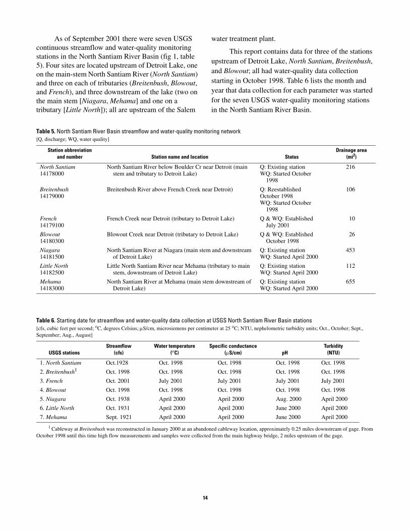
Erosion and Suspended Sediment

Erosion and sediment transport are likely related to landscape, geomorphic characteristics, tectonic uplift, seismic events, and land use. For instance, because the North Santiam River Basin upstream of Detroit Lake is approximately 98 percent forested (fig. 3; U.S. Geological Survey, 1990), practices associated with timber harvesting, such as road building and logging operations, may alter storm hydrographs and increase sediment delivery to streams (Harr et al.,

Debris flow in Ivy Creek, just upstream of Blowout station, caused by road washout.

12

1975; Swanson and Dryness, 1975). Since 1960, approximately 21 percent of U.S. Forest Service lands have been harvested above Detroit Lake (Cotton et al., 1998). Clearcutting has been shown to alter snow accumulation and melting and cause increased peak streamflows during rainfall, thereby increasing the potential for hillslope and/or channel erosion (Harris, 1977; Harr, 1986). Unpaved road surfaces also may act as important sediment sources to rivers (Reid and Dunne, 1984; Bilby, 1985).

The North Santiam River Basin extends eastward to the crest of the Cascade Range to elevations above 8,000 feet. These areas are glaciated and prone to landslides, mass wasting, and water outburst events causing channel alterations that can substantially affect the sediment carrying capacity of the local streams, as well as the relation between suspended sediment and streamflow (Walder and Driedger, 1994). Volcanic events in the Cascade Range can also cause extreme shifts in sediment flux, such as at Mount St. Helens, Washington, where sediment yields increased by as much as 500 times the pre-eruption background levels before 1980 (Major et al., 2000).

METHODS OF INVESTIGATION

Monitoring Network

Major tributaries to Detroit Lake and the North Santiam River, along with the main-stem North Santiam River and the outflow from Detroit Lake, were selected for streamflow and water-quality monitoring sites. Tributary monitoring sites were located as near to the tributary mouth as practicable in order to represent the largest drainage area of the subbasin. Existing USGS gaging stations were used wherever possible.

Historic Gaging Stations

Four long-term USGS stream-gaging stations in the North Santiam River Basin were in operation at the start of this study in October 1998. These stations were selected as part of the water-quality network because of their long-term streamflow record, location upstream of the Salem water treatment facility, and minimal construction requirements, since installation was already complete. Also considered was a location near a watershed’s farthest point downstream and/or a site

on a stream entering or exiting Detroit Lake. The long-term stations include (fig. 1):

1. North Santiam River at Mehama (Mehama, 14183000; begun 1921),

2. Little North Santiam River near Mehama (Little North, 14182500; begun 1931).

3. North Santiam River at Niagara (Niagara, 14181500; begun 1938),

4. North Santiam River below Boulder Creek near Detroit (North Santiam, 14178000; begun 1928)

All historic stations provided continuous (30 minute and/or hourly) streamflow data which are published as a daily mean discharge. Breitenbush River above French Creek near Detroit (Breitenbush, 14179000), entering Detroit Lake from the north, is also a historic-record site. Breitenbush continuous streamflow record was available only from 1933 through 1987, at which time the station was discontinued. The Breitenbush gage was reestablished in October 1998 and was added to the study network. In addition, historic continuous water temperature data is available for all sites (North Santiam and Breitenbush, 1951–87; Niagara, 1954–97; Mehama and Little North, 1986 only). Besides water temperature data, no other continuous water-quality data were collected at these five sites.

Active Water-Quality Stations

The turbidity in Detroit Lake caused by the events of February 1996 prompted continuous monitoring of water quality in streams flowing into the lake. In October 1998, in addition to streamflow, the collection of continuous four-parameter water-quality data was begun upstream of Detroit Lake at North Santiam and Breitenbush. The parameters measured include water temperature, specific conductance, pH, and turbidity, collected in 30-minute intervals, which match the streamflow-data collection times. Also in October 1998, an identical continuous streamflow and water-quality station was installed upstream and south of Detroit Lake at Blowout Creek near Detroit (Blowout, 14180300) (fig. 1).

In April 2000, in order to monitor water-quality downstream of Detroit Lake, the USGS stream-gaging stations of Niagara, Little North, and Mehama also began collecting continuous four-parameter water-quality data. Finally, in July 2001, a continuous stream-gaging and water-quality monitoring station was added on a small watershed upstream and north of Detroit Lake at French Creek near Detroit (French).

13

As of September 2001 there were seven USGS water treatment plant. continuous streamflow and water-quality monitoring This report contains data for three of the stations stations in the North Santiam River Basin (fig 1, table 5). Four sites are located upstream of Detroit Lake, one

upstream of Detroit Lake, North Santiam, Breitenbush,

on the main-stem North Santiam River (North Santiam) and Blowout; all had water-quality data collection

and three on each of tributaries (Breitenbush, Blowout, starting in October 1998. Table 6 lists the month and

and French), and three downstream of the lake (two on year that data collection for each parameter was started

the main stem [Niagara, Mehama] and one on a for the seven USGS water-quality monitoring stations tributary [Little North]); all are upstream of the Salem in the North Santiam River Basin.

Table 5. North Santiam River Basin streamflow and water-quality monitoring network [Q, discharge; WQ, water quality]

Station abbreviation Drainage area and number Station name and location Status (mi2)

North Santiam North Santiam River below Boulder Cr near Detroit (main Q: Existing station 216 14178000 stem and tributary to Detroit Lake) WQ: Started October

1998

Breitenbush Breitenbush River above French Creek near Detroit) Q: Reestablished 106 14179000 October 1998

WQ: Started October 1998

French French Creek near Detroit (tributary to Detroit Lake) Q & WQ: Established 10 14179100 July 2001

Blowout Blowout Creek near Detroit (tributary to Detroit Lake) Q & WQ: Established 26 14180300 October 1998

Niagara North Santiam River at Niagara (main stem and downstream Q: Existing station 453 14181500 of Detroit Lake) WQ: Started April 2000

Little North Little North Santiam River near Mehama (tributary to main Q: Existing station 112 14182500 stem, downstream of Detroit Lake) WQ: Started April 2000

Mehama North Santiam River at Mehama (main stem downstream of Q: Existing station 655 14183000 Detroit Lake) WQ: Started April 2000

Table 6. Starting date for streamflow and water-quality data collection at USGS North Santiam River Basin stations [cfs, cubic feet per second; oC, degrees Celsius; µS/cm, microsiemens per centimeter at 25 oC; NTU, nephelometric turbidity units; Oct., October; Sept., September; Aug., August]

USGS stations Streamflow

(cfs) Water temperature

(οC) Specific conductance

(µS/cm) pH Turbidity

(NTU)

1. North Santiam Oct.1928 Oct. 1998 Oct. 1998 Oct. 1998 Oct. 1998

2. Breitenbush1 Oct. 1998 Oct. 1998 Oct. 1998 Oct. 1998 Oct. 1998

3. French Oct. 2001 July 2001 July 2001 July 2001 July 2001

4. Blowout Oct. 1998 Oct. 1998 Oct. 1998 Oct. 1998 Oct. 1998

5. Niagara Oct. 1938 April 2000 April 2000 Aug. 2000 April 2000

6. Little North Oct. 1931 April 2000 April 2000 June 2000 April 2000

7. Mehama Sept. 1921 April 2000 April 2000 June 2000 April 2000

1 Cableway at Breitenbush was reconstructed in January 2000 at an abandoned cableway location, approximately 0.25 miles downstream of gage. From October 1998 until this time high flow measurements and samples were collected from the main highway bridge, 2 miles upstream of the gage.

14

Data Collection

Site Instrumentation

All seven sites have separate stream-stage and YSI multiparameter water-quality datasondes installed. All sites are telemetered via direct phone lines, except Blowout and French, which have a cellular telephone system. Data are recorded every 30 minutes on a separate data logger. The datasondes also have data logging capabilities and record data in 15 minute intervals, providing redundancy to the primary data collection system. The direct-line sites are called at 3-hour intervals (8 times per day) for data retrieval. The cellular phone sites are called six times per day at 4-hour intervals. A depth sensor on the YSI datasonde supplies backup stage data for all sites.

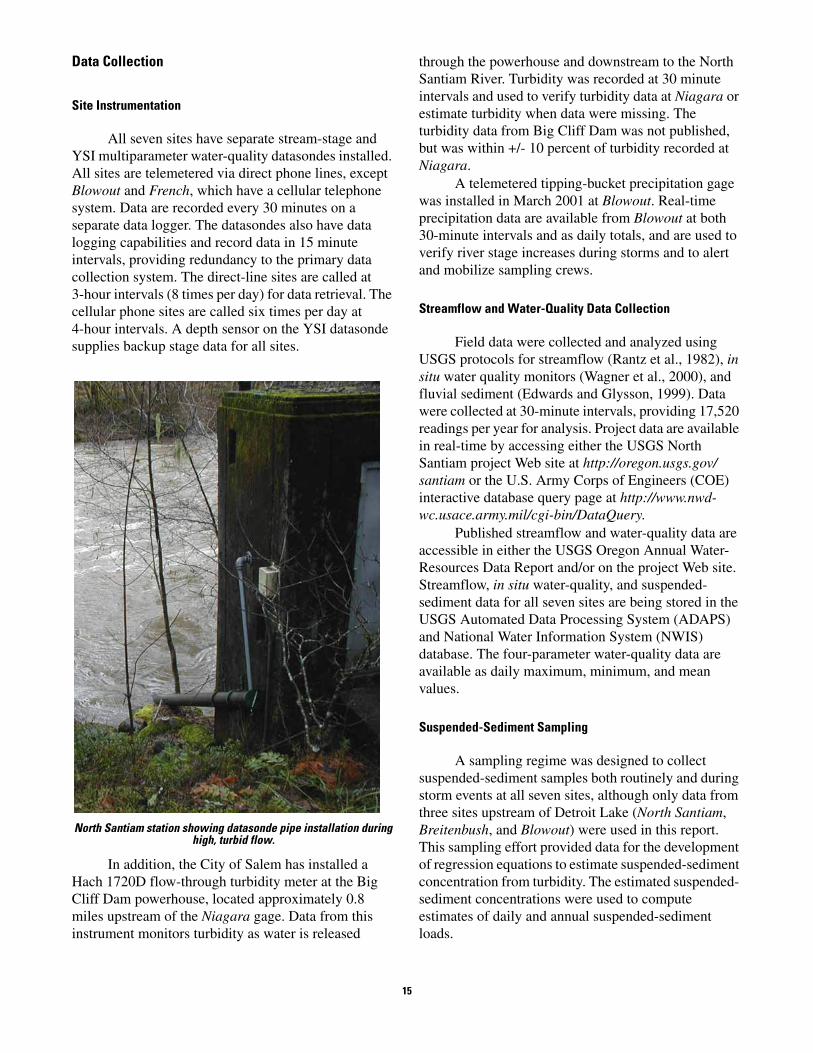
North Santiam station showing datasonde pipe installation during high, turbid flow.

In addition, the City of Salem has installed a Hach 1720D flow-through turbidity meter at the Big Cliff Dam powerhouse, located approximately 0.8 miles upstream of the Niagara gage. Data from this instrument monitors turbidity as water is released

through the powerhouse and downstream to the North Santiam River. Turbidity was recorded at 30 minute intervals and used to verify turbidity data at Niagara or estimate turbidity when data were missing. The turbidity data from Big Cliff Dam was not published, but was within +/- 10 percent of turbidity recorded at Niagara.

A telemetered tipping-bucket precipitation gage was installed in March 2001 at Blowout. Real-time precipitation data are available from Blowout at both 30-minute intervals and as daily totals, and are used to verify river stage increases during storms and to alert and mobilize sampling crews.

Streamflow and Water-Quality Data Collection

Field data were collected and analyzed using USGS protocols for streamflow (Rantz et al., 1982), in situ water quality monitors (Wagner et al., 2000), and fluvial sediment (Edwards and Glysson, 1999). Data were collected at 30-minute intervals, providing 17,520 readings per year for analysis. Project data are available in real-time by accessing either the USGS North Santiam project Web site at http://oregon.usgs.gov/ santiam or the U.S. Army Corps of Engineers (COE) interactive database query page at http://www.nwd- wc.usace.army.mil/cgi-bin/DataQuery.

Published streamflow and water-quality data are accessible in either the USGS Oregon Annual Water-Resources Data Report and/or on the project Web site. Streamflow, in situ water-quality, and suspended- sediment data for all seven sites are being stored in the USGS Automated Data Processing System (ADAPS) and National Water Information System (NWIS) database. The four-parameter water-quality data are available as daily maximum, minimum, and mean values.

Suspended-Sediment Sampling

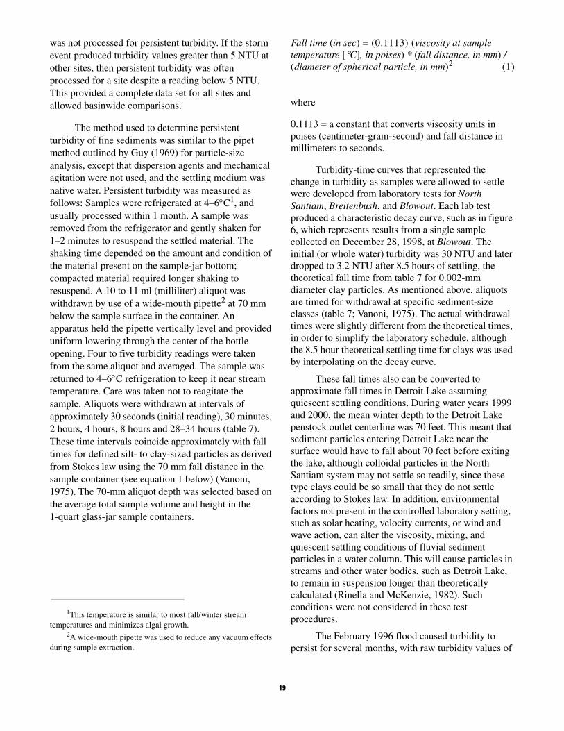
A sampling regime was designed to collect suspended-sediment samples both routinely and during storm events at all seven sites, although only data from three sites upstream of Detroit Lake (North Santiam, Breitenbush, and Blowout) were used in this report. This sampling effort provided data for the development of regression equations to estimate suspended-sediment concentration from turbidity. The estimated suspended- sediment concentrations were used to compute estimates of daily and annual suspended-sediment loads.

15

Fine clay particles are washed from the upper tributary watersheds to the water column of Detroit Lake and delta areas, where they either settle to the lake bottom or are carried through the reservoir and released downstream (Bates et al., 1998). To estimate the magnitude of the larger (heavier) and smaller (lighter) fractions of the suspended-sediment load, and therefore the faster to slower particle settling ratio, the suspended-sediment analysis included a sand-silt (coarse/fine) partitioning by either a wet- or dry-sieve method (Guy, 1969). This process separates particles smaller than 0.062 mm nominal diameter (clay and silt) from those that are larger than or equal to 0.062 mm (sand and larger particles) (Colby, 1963). This coarse/ fine separation facilitates the study of fluvial sediment transport dynamics and can be used to pinpoint sources of high and persistent turbidity in specific subbasins of the North Santiam tributary-reservoir system. Samples were analyzed for total sediment concentration and for sand-silt partitioning when sand was present, as explained above. In addition, the clay fraction was determined from samples with higher sediment content, usually collected during one or two high rainfall events per site per year, or more frequently if sufficient fine particles were present. Fine-particle analysis was performed by using millimeter sieve sizes of 0.031, 0.016, 0.008, 0.004, and 0.002. Results from these samples could help to provide a characterization of the clay types and quantify the amount of fine material from each subbasin. This data could be correlated to the persistent-turbidity information as a method to verify clay water estimates (see Persistent-Turbidity Sampling and Processing).

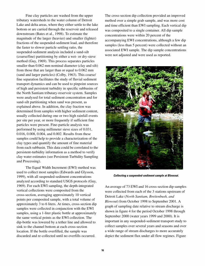
The Equal Width Increment (EWI) method was used to collect most samples (Edwards and Glysson, 1999), with all suspended-sediment concentrations analyzed according to standard USGS protocols (Guy, 1969). For each EWI sampling, the depth-integrated vertical collections were composited from the cross-section, averaging approximately 10 vertical points per composited sample, with a total volume of approximately 3 to 6 liters. At times, cross-section dip samples were collected in conjunction with the EWI samples, using a 1-liter plastic bottle at approximately the same vertical points as the EWI collection. The dip-bottle was lowered by a tether line and allowed to sink to the channel bottom at each cross-section location. If the bottle overfilled, the sample was discarded and re-collected until no overfills occurred.

The cross-section dip collection provided an improved method over a simple grab sample, and was more cost and time efficient than EWI sampling. Each vertical dip was composited to a single container. All dip sample concentrations were within 20 percent of the accompanying EWI concentrations, although a few dip samples (less than 5 percent) were collected without an associated EWI sample. The dip sample concentrations were not adjusted and were used as reported.

Collecting a suspended-sediment sample at Blowout.

An average of 73 EWI and 16 cross-section dip samples were collected from each of the 3 stations upstream of Detroit Lake (North Santiam, Breitenbush, and Blowout) from October 1998 to September 2001. A graph of sampling date relative to stream discharge is shown in figure 4 for the period October 1998 through September 2000 (water years 1999 and 2000). It is important in any suspended-sediment transport study to collect samples over several years and seasons and over a wide range of stream discharges to more accurately depict the sediment flux under all flow regimes. Figure

16

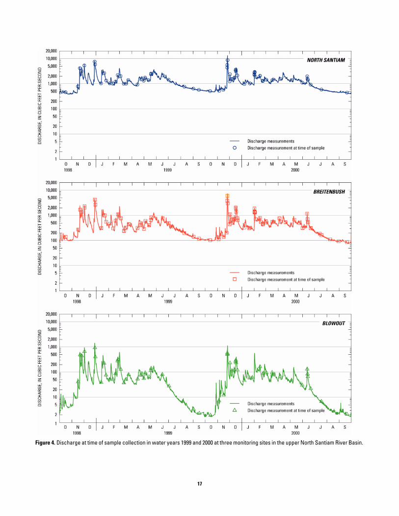
Figure 4. Discharge at time of sample collection in water years 1999 and 2000 at three monitoring sites in the upper North Santiam River Basin.

17

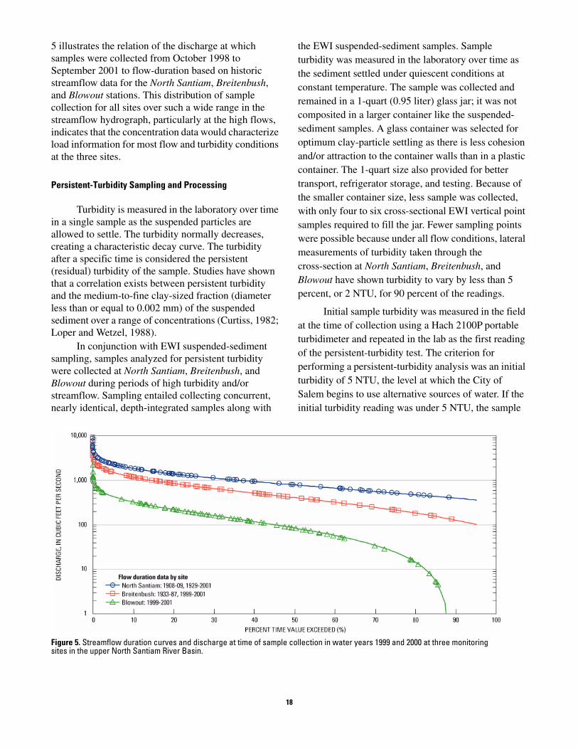
5 illustrates the relation of the discharge at which samples were collected from October 1998 to September 2001 to flow-duration based on historic streamflow data for the North Santiam, Breitenbush, and Blowout stations. This distribution of sample collection for all sites over such a wide range in the streamflow hydrograph, particularly at the high flows, indicates that the concentration data would characterize load information for most flow and turbidity conditions at the three sites.

Persistent-Turbidity Sampling and Processing

Turbidity is measured in the laboratory over time in a single sample as the suspended particles are allowed to settle. The turbidity normally decreases, creating a characteristic decay curve. The turbidity after a specific time is considered the persistent (residual) turbidity of the sample. Studies have shown that a correlation exists between persistent turbidity and the medium-to-fine clay-sized fraction (diameter less than or equal to 0.002 mm) of the suspended sediment over a range of concentrations (Curtiss, 1982; Loper and Wetzel, 1988).

In conjunction with EWI suspended-sediment sampling, samples analyzed for persistent turbidity were collected at North Santiam, Breitenbush, and Blowout during periods of high turbidity and/or streamflow. Sampling entailed collecting concurrent, nearly identical, depth-integrated samples along with

the EWI suspended-sediment samples. Sample turbidity was measured in the laboratory over time as the sediment settled under quiescent conditions at constant temperature. The sample was collected and remained in a 1-quart (0.95 liter) glass jar; it was not composited in a larger container like the suspended- sediment samples. A glass container was selected for optimum clay-particle settling as there is less cohesion and/or attraction to the container walls than in a plastic container. The 1-quart size also provided for better transport, refrigerator storage, and testing. Because of the smaller container size, less sample was collected, with only four to six cross-sectional EWI vertical point samples required to fill the jar. Fewer sampling points were possible because under all flow conditions, lateral measurements of turbidity taken through the cross-section at North Santiam, Breitenbush, and Blowout have shown turbidity to vary by less than 5 percent, or 2 NTU, for 90 percent of the readings.

Initial sample turbidity was measured in the field at the time of collection using a Hach 2100P portable turbidimeter and repeated in the lab as the first reading of the persistent-turbidity test. The criterion for performing a persistent-turbidity analysis was an initial turbidity of 5 NTU, the level at which the City of Salem begins to use alternative sources of water. If the initial turbidity reading was under 5 NTU, the sample

Figure 5. Streamflow duration curves and discharge at time of sample collection in water years 1999 and 2000 at three monitoring sites in the upper North Santiam River Basin.

18

was not processed for persistent turbidity. If the storm event produced turbidity values greater than 5 NTU at other sites, then persistent turbidity was often processed for a site despite a reading below 5 NTU. This provided a complete data set for all sites and allowed basinwide comparisons.

The method used to determine persistent turbidity of fine sediments was similar to the pipet method outlined by Guy (1969) for particle-size analysis, except that dispersion agents and mechanical agitation were not used, and the settling medium was native water. Persistent turbidity was measured as follows: Samples were refrigerated at 4–6°C1, and usually processed within 1 month. A sample was removed from the refrigerator and gently shaken for 1–2 minutes to resuspend the settled material. The shaking time depended on the amount and condition of the material present on the sample-jar bottom; compacted material required longer shaking to resuspend. A 10 to 11 ml (milliliter) aliquot was withdrawn by use of a wide-mouth pipette2 at 70 mm below the sample surface in the container. An apparatus held the pipette vertically level and provided uniform lowering through the center of the bottle opening. Four to five turbidity readings were taken from the same aliquot and averaged. The sample was returned to 4–6°C refrigeration to keep it near stream temperature. Care was taken not to reagitate the sample. Aliquots were withdrawn at intervals of approximately 30 seconds (initial reading), 30 minutes, 2 hours, 4 hours, 8 hours and 28–34 hours (table 7). These time intervals coincide approximately with fall times for defined silt- to clay-sized particles as derived from Stokes law using the 70 mm fall distance in the sample container (see equation 1 below) (Vanoni, 1975). The 70-mm aliquot depth was selected based on the average total sample volume and height in the 1-quart glass-jar sample containers.

1This temperature is similar to most fall/winter stream temperatures and minimizes algal growth.

2A wide-mouth pipette was used to reduce any vacuum effects during sample extraction.

Fall time (in sec) = (0.1113) (viscosity at sample temperature [°C], in poises) * (fall distance, in mm) / (diameter of spherical particle, in mm)2 (1)

where

0.1113 = a constant that converts viscosity units in poises (centimeter-gram-second) and fall distance in millimeters to seconds.

Turbidity-time curves that represented the change in turbidity as samples were allowed to settle were developed from laboratory tests for North Santiam, Breitenbush, and Blowout. Each lab test produced a characteristic decay curve, such as in figure 6, which represents results from a single sample collected on December 28, 1998, at Blowout. The initial (or whole water) turbidity was 30 NTU and later dropped to 3.2 NTU after 8.5 hours of settling, the theoretical fall time from table 7 for 0.002-mm diameter clay particles. As mentioned above, aliquots are timed for withdrawal at specific sediment-size classes (table 7; Vanoni, 1975). The actual withdrawal times were slightly different from the theoretical times, in order to simplify the laboratory schedule, although the 8.5 hour theoretical settling time for clays was used by interpolating on the decay curve.

These fall times also can be converted to approximate fall times in Detroit Lake assuming quiescent settling conditions. During water years 1999 and 2000, the mean winter depth to the Detroit Lake penstock outlet centerline was 70 feet. This meant that sediment particles entering Detroit Lake near the surface would have to fall about 70 feet before exiting the lake, although colloidal particles in the North Santiam system may not settle so readily, since these type clays could be so small that they do not settle according to Stokes law. In addition, environmental factors not present in the controlled laboratory setting, such as solar heating, velocity currents, or wind and wave action, can alter the viscosity, mixing, and quiescent settling conditions of fluvial sediment particles in a water column. This will cause particles in streams and other water bodies, such as Detroit Lake, to remain in suspension longer than theoretically calculated (Rinella and McKenzie, 1982). Such conditions were not considered in these test procedures.

The February 1996 flood caused turbidity to persist for several months, with raw turbidity values of

19

Table 7. Fall times for suspended-sediment particles and schedule for aliquot withdrawals (at 4 degrees Celsius) mm, millimeters

Theoretical fall time

Class name Particle size

diameter for 70 mm

(in laboratory) Actual laboratory aliquot

withdrawal schedule Theoretical fall time for

70 feet (in lake)

Coarse to medium silt 0.062 mm 34 seconds Initial after shaking 2.7 minutes Fine to very fine silt .008 mm 32 minutes 30 minutes 6.7 days Very fine silt to coarse clay .004 mm 2.1 hours 2 hours 26.9 days Coarse clay .003 mm 3.8 hours 4 hours 47.8 days Medium to fine clay .002 mm 8.5 hours 8 hours 107.7 days (3.5 months) Fine clay .001 mm 34 hours 28-34 hours 1.2 years Very fine clay .0005 mm 5.7 days 5–6 days 4.7 years

Figure 6. Turbidity decay curve for sample collected December 29, 1998, at Blowout Creek sampling station.

10 NTU recorded into the summer at the intakes of the Salem water treatment plant. Because fall times are directly correlated to specific sediment sizes, each class of clay-sized particle will correspond to an approximate turbidity at a given settling time during the testing sequence. By using table 7 and the February 1996 data, persistent turbidity in Detroit Lake can be characterized as the time it took 0.002 mm size particles and smaller to settle as much as 70 feet and exit through the Detroit Lake outlet port. This equates to approximately 3.5 months or longer at 4°C (fig. 7), which was about the length of time the high turbidity persisted in Detroit Lake and downstream to the treatment plant after February 1996.

Detroit Lake Persistent-Turbidity Sampling

Persistent-turbidity samples were collected from Detroit Lake by the U.S. Army Corps of Engineers after three storm events during 1998 and 1999. Three locations in Detroit Lake were sampled: (1) close to

Detroit Dam near the log boom, (2) near the Blowout Creek tributary inflow, and (3) upstream and adjacent to Piety Island near Mongold State Park and the tributary inflows of the North Santiam River, Breiten- bush River, and French Creek. Samples for persistent turbidity were collected with a VanDorn sampler. Sampling depths generally were at two points in the vertical profile: near the surface and close to the lake bottom. Lake and tributary persistent turbidity were compared.

Quality Assurance

Data Collection

As a means of quality assurance, standard USGS methods and protocols were used for all measurements, sampling, and data-management activities. These included stream discharge measurements, suspended-sediment sampling and analysis, and data management and review (Rantz et al., 1982; Edwards and Glysson, 1999). Duplicate suspended-sediment samples were collected and analyzed to determine the precision of the results from the sediment lab. Approximately 15 percent of the total number of suspended-sediment samples processed at all sites were collected as duplicate EWI or dip samples. Almost all duplicate suspended-sediment concentrations were within 20 percent of the corresponding sample suspended-sediment concentrations, although this difference was usually less, especially for higher concentrations, such as for most high-flow samples. That is, hypothetically because the concentration differences between duplicate low-flow samples with concentrations of 1 and 1.2 mg/l (milligrams per liter) and high-flow concentrations of 100 and 120 mg/l both equate to a 20

20

Figure 7. Theoretical fall distances at 4 degrees Celsius for different fine-particle sizes at selected time intervals in Detroit Lake reservoir, Oregon.

21

percent difference, duplicate samples collected during high-flow can differ by a greater amount than samples collected during low-flow and still have concentrations within 20 percent. Double-blind samples also were prepared by an independent laboratory and submitted to the processing sediment laboratory to verify suspended-sediment concentrations and sand/fine particle percentages.

Instrument Calibration

Extensive inhouse protocols were developed to calibrate the instream datasondes, along with using existing USGS procedures for continuous water-quality monitors (Wagner et al., 2000). Each calibration required readings from both the existing datasonde and a second datasonde brought to the site. Both datasondes are calibrated onsite with standards at a temperature near that of the stream. The second datasonde is placed in the water next to the station datasonde and allowed to equilibrate; duplicate readings are taken from each water-quality monitor. The second datasonde is used to monitor changes in the stream during the calibration period and as an approximate check of the station datasonde readings. Datasonde calibration occurs every 2–3 weeks at all sites and may either coincide with the suspended-sediment sampling or occur on a separate trip. Cross-sectional measurements generally accompanied each calibration visit, which included attaining readings with the backup datasonde from at least three points in the cross-section and comparing those readings to readings from the station datasonde. In addition, separate turbidity dip cuvette samples, near the datasonde instream location, were collected during all datasonde calibrations and measured onsite with a Hach 2100P and compared to the station turbidity readings.

Data Calculations

Suspended-Sediment Load Calculations

To calculate suspended-sediment load (SSL), the estimates of suspended-sediment concentrations (SSC) were first derived from the instream turbidity-monitor

Calibrating datasonde at Blowout.

data for each of the three stations and corresponding subbasins using least squares regression. The SSC values from each of the equal-width increment (EWI) and dip samples are plotted against turbidity (in NTU) in figure 8A. The turbidity value used was averaged from the 30-minute instream data over the time of sample collection. Since the mid-1950’s, streamflow has been the common parameter used to estimate SSC (Colby, 1963). Hence, as a comparison to turbidity, streamflow also was evaluated as a surrogate for SSC (fig. 8B). Both predictor values (turbidity or Q) and the response variable SSC are normalized by log transformation to better fit the data to the regression line and then converted to a power-function equation using ordinary least-squares regression. These equations can be expressed as:

log SSC = log a + b log (turbidity or Q), (2)

which is converted to:

22

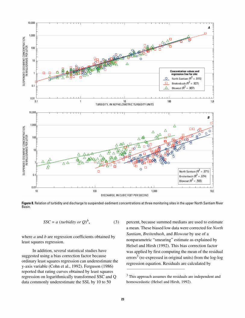
Figure 8. Relation of turbidity and discharge to suspended-sediment concentrations at three monitoring sites in the upper North Santiam River Basin.

SSC = a (turbidity or Q)b , (3) percent, because summed medians are used to estimate a mean. These biased low data were corrected for North Santiam, Breitenbush, and Blowout by use of a

where a and b are regression coefficients obtained by least squares regression.

In addition, several statistical studies have suggested using a bias correction factor because

nonparametric “smearing” estimate as explained by Helsel and Hirsh (1992). This bias correction factor was applied by first computing the mean of the residual errors3 (re-expressed in original units) from the log-log

ordinary least squares regression can underestimate the regression equation. Residuals are calculated by y-axis variable (Cohn et al., 1992). Ferguson (1986) reported that rating curves obtained by least squares regression on logarithmically transformed SSC and Q 3 This approach assumes the residuals are independent and data commonly underestimate the SSL by 10 to 50 homoscedastic (Helsel and Hirsh, 1992).

23

----------------

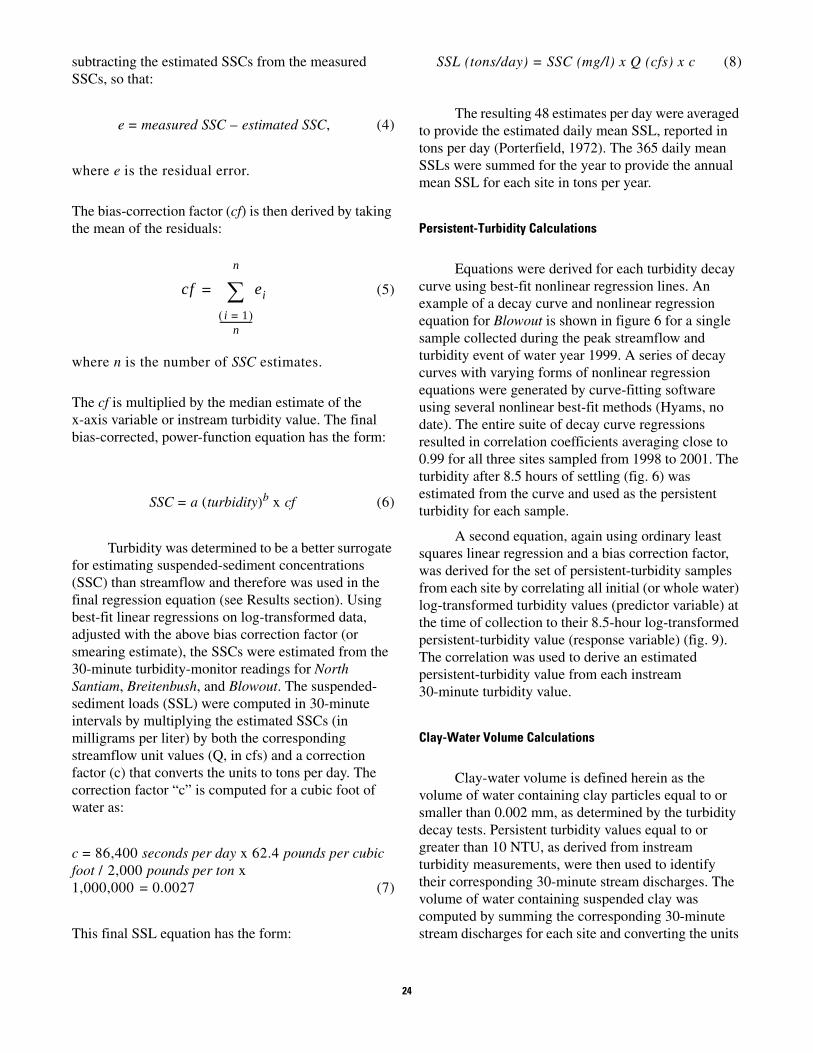
subtracting the estimated SSCs from the measured SSCs, so that:

e = measured SSC – estimated SSC, (4)

where e is the residual error.

The bias-correction factor (cf) is then derived by taking the mean of the residuals:

n

cf = ∑ ei (5)

(i = 1) n

where n is the number of SSC estimates.

The cf is multiplied by the median estimate of the x-axis variable or instream turbidity value. The final bias-corrected, power-function equation has the form:

SSC = a (turbidity)b x cf (6)

Turbidity was determined to be a better surrogate for estimating suspended-sediment concentrations (SSC) than streamflow and therefore was used in the final regression equation (see Results section). Using best-fit linear regressions on log-transformed data, adjusted with the above bias correction factor (or smearing estimate), the SSCs were estimated from the 30-minute turbidity-monitor readings for North Santiam, Breitenbush, and Blowout. The suspended- sediment loads (SSL) were computed in 30-minute intervals by multiplying the estimated SSCs (in milligrams per liter) by both the corresponding streamflow unit values (Q, in cfs) and a correction factor (c) that converts the units to tons per day. The correction factor “c” is computed for a cubic foot of water as:

c = 86,400 seconds per day x 62.4 pounds per cubic foot / 2,000 pounds per ton x 1,000,000 = 0.0027 (7)

This final SSL equation has the form:

SSL (tons/day) = SSC (mg/l) x Q (cfs) x c (8)

The resulting 48 estimates per day were averaged to provide the estimated daily mean SSL, reported in tons per day (Porterfield, 1972). The 365 daily mean SSLs were summed for the year to provide the annual mean SSL for each site in tons per year.

Persistent-Turbidity Calculations

Equations were derived for each turbidity decay curve using best-fit nonlinear regression lines. An example of a decay curve and nonlinear regression equation for Blowout is shown in figure 6 for a single sample collected during the peak streamflow and turbidity event of water year 1999. A series of decay curves with varying forms of nonlinear regression equations were generated by curve-fitting software using several nonlinear best-fit methods (Hyams, no date). The entire suite of decay curve regressions resulted in correlation coefficients averaging close to 0.99 for all three sites sampled from 1998 to 2001. The turbidity after 8.5 hours of settling (fig. 6) was estimated from the curve and used as the persistent turbidity for each sample.

A second equation, again using ordinary least squares linear regression and a bias correction factor, was derived for the set of persistent-turbidity samples from each site by correlating all initial (or whole water) log-transformed turbidity values (predictor variable) at the time of collection to their 8.5-hour log-transformed persistent-turbidity value (response variable) (fig. 9). The correlation was used to derive an estimated persistent-turbidity value from each instream 30-minute turbidity value.

Clay-Water Volume Calculations

Clay-water volume is defined herein as the volume of water containing clay particles equal to or smaller than 0.002 mm, as determined by the turbidity decay tests. Persistent turbidity values equal to or greater than 10 NTU, as derived from instream turbidity measurements, were then used to identify their corresponding 30-minute stream discharges. The volume of water containing suspended clay was computed by summing the corresponding 30-minute stream discharges for each site and converting the units

24

Figure 9. Relation of persistent turbidity to initial turbidity at three monitoring sites in the upper North Santiam River Basin in water years 1999 and 2000.

to million gallons per year. The percentage of the total volume of water entering Detroit Lake in 1999 and 2000 from the three major tributaries (North Santiam, Breitenbush, and Blowout) estimated to be clay water also was calculated.

RESULTS

Estimated Annual Suspended-Sediment Loads

The equations relating streamflow to suspended-sediment concentration for the North Santiam, Breitenbush, and Blowout sites for water years 1999 and 2000 are shown in table 8. This power model form of the equation retransforms the x and y variables from the log-log least-squares regression back to the original units. The linear plots in figure 8B illustrate the widespread scatter of streamflow and suspended-sediment concentration data around the regression lines.

As a comparison, turbidity was used as the predictor variable, replacing streamflow, in a similar least-squares regression with the response variable of suspended-sediment concentration. The resulting linear regressions for North Santiam, Breitenbush, and Blowout are shown in figure 8A. The turbidity and suspended-sediment concentration graph clearly shows better correlation than the streamflow and suspended- sediment concentration graph. This is further con

firmed by the higher coefficient of determination (R2) and lower standard error of estimate (SE) values for these lines. Table 9 lists power-function equations using turbidity (predictor variable) and suspended- sediment concentration (response variable) data, retransformed to original units, for North Santiam, Breitenbush, and Blowout. The regression equations in tables 8 and 9 include the bias correction factor applied using the “smearing” estimate approach described in the Methods of Investigation section.

The median estimate of turbidity from the power model equation is multiplied by the bias correction factor to generate a slightly higher regression line in relation to the original, unmodified line. In figure 10, each of the three original and bias-corrected regression lines are shown separately for each site for the turbidity versus suspended-sediment concentrations relations.

Figure 10 also shows the 95 percent prediction intervals for each regression equation. Few sampling points are outside of the prediction intervals, hence there is a near 95 percent certainty that subsequent turbidity versus suspended-sediment concentration (SSC) values will fall within these regression bands.

The suspended-sediment load (SSL) estimates for each of the sites for water years 1999 and 2000 are shown in figure 11. The estimated water year 1999 SSL values for the three sites were similar, ranging from approximately 20,100 tons for Breitenbush to 15,000 tons for Blowout, with North Santiam between. The difference between Breitenbush and Blowout was 5,100 tons, or 25 percent of the Breitenbush load.

25

Table 8. Power regression equations for estimating suspended-sediment concentrations (SSC) from streamflow data (Q)

Station Power model equation R2 and standard error

North Santiam SSC = 6.60E-05 * Q1.58 * (1.62, Bias Correction Factor) R2 = 0.565 SE = 35.2

Breitenbush SSC = 9.54E-05 * Q1.66 * (1.84, Bias Correction Factor) R2 = 0.674 SE = 90.1

Blowout SSC = 2.82E-02 * Q1.05 * (1.64, Bias Correction Factor) R2 = 0.671 SE = 83.4

Table 9. Power regression equations for estimating suspended-sediment concentrations (SSC) from instream turbidity-monitor data (T)

Station Power model equation R2 and standard error

North Santiam (SSC) = 1.70 * T1.04 * (1.10, Bias Correction Factor) R2 = 0.912 SE = 33.2

Breitenbush (SSC) = 1.85 * T0.988 * (1.17, Bias Correction Factor) R2 = 0.948 SE = 39.3

Blowout (SSC) = 1.45 * T1.08 * (1.13, Bias Correction Factor) R2 = 0.964 SE = 30.1

In water year 2000 the basin SSLs followed the same trend; however, there was a much wider discrepancy between the basins. The annual SSL for Breitenbush exceeded the value for North Santiam by over 180 percent and Blowout by almost 930 percent, with a difference between the largest and smallest SSL of 45,500 tons, or 90 percent of the Breitenbush load.

To further illustrate the disparity among basins, bar graphs of SSLs are shown in figure 11 for the peak 3-day streamflow/turbidity events for both years. The instantaneous peak values for turbidity and suspended-sediment load during these storms are listed in table 10. Each 3-day storm period accounted for greater than 50 percent of the annual SSL for all sites and years, except for North Santiam in 1999. For example, the 3-day storm event of December 27–29, 1998, in water year 1999, accounted for 40, 63, and 64 percent of the annual load at North Santiam, Breitenbush, and Blowout, respectively. The peak turbidity ranged from 198 NTU at North Santiam to 1,049 NTU at Breitenbush, with Blowout in between at 875 NTU (fig. 12 [p. 29]).

The 3-day storm event that took place November 25–27, 1999, in water year 2000, accounted for over 75 percent of the annual suspended-sediment production for all three sites in that year, ranging from 76 percent for Blowout to 91 percent for Breitenbush (table 10 [p. 29]). The turbidity value at Breitenbush peaked at 1,160 NTU during this storm and remained greater than 200 NTU for 37 hours. Turbidity at Blowout peaked at 1,310 NTU and remained greater than 200

NTU for only 90 minutes, and at North Santiam peaked at only 739 NTU and remained above 200 NTU for 24 hours (fig. 12). The higher value and longer duration of the turbidity peak at Breitenbush clearly accounts for the greater SSL for the water year 2000 storm event. Additionally, since Breitenbush recorded the highest SSL during both of these storm events, it is possible the production of suspended-sediment in this basin may be more highly storm-driven than in the other two basins, possibly because of more glacial activity, snowmelt, a slope or larger bank and/or road failure in the upper part of the watershed. The high, short duration turbidity peak at Blowout in 2000 may also indicate some type of bank failure, though of smaller extent.

The measured and estimated SSCs for each sample are shown in figure 13 (p. 30). The slopes of the best-fit SSC linear regressions for each site demon- strate good agreement (+/- 20 percent) of the estimated values with the measured values over a wide range of SSCs, especially at the more crucial higher concentrations. In addition, figure 14 (p. 31) shows the result of using these estimated SSCs in graphing the average daily SSL values estimated from turbidity relative to the measured SSL values from the samples collected for water years 1999 and 2000. Again the estimated daily SSLs closely overlay the measured SSLs, particularly at the higher SSLs, although some estimated SSLs of 1 ton or less overestimate SSL. Additional suspended- sediment samples are needed at lower SSCs, which may require a different turbidity

26

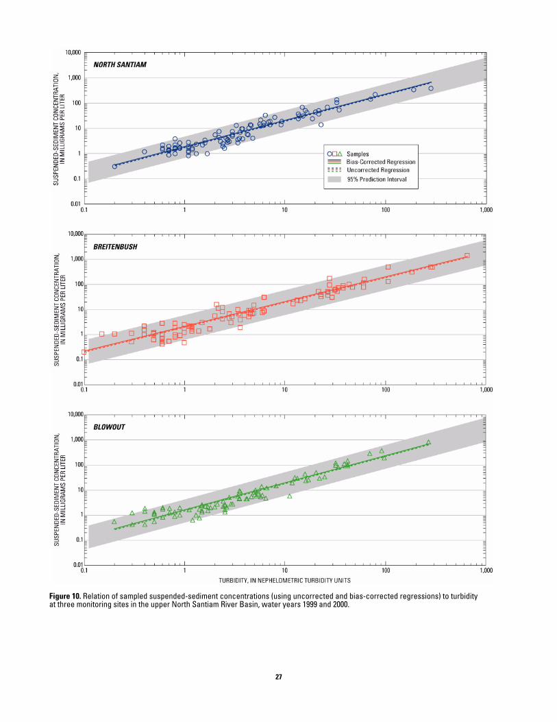
Figure 10. Relation of sampled suspended-sediment concentrations (using uncorrected and bias-corrected regressions) to turbidity at three monitoring sites in the upper North Santiam River Basin, water years 1999 and 2000.

27

Figure 11. Estimated annual and peak storm suspended-sediment loads at three monitoring sites in the upper North Santiam River Basin, water years 1999 and 2000.

SSC regression, to minimize this discrepancy at lower SSLs.

To further compare SSLs from the three sites, figure 15 (p. 32) uses a logarithmic scale boxplot to show the distribution of daily mean estimated SSL. Blowout had a lower median SSL but more widely varying interquartile range (25th and 75th percentile) for both water years 1999 and 2000. North Santiam had the highest median but least variability of the three sites for both years. This suggests that in water years 1999 and 2000, the sediment and clay sources in the Blowout and Breitenbush subbasins were more highly variable and prone to storm-induced landslide and channel alterations than the basin upstream of North Santiam.

Figure 15 shows that the mean value was higher than the median for all sites and years, indicating a nonnormal distribution of the data. The 1999 means are similar, although Blowout was the highest at 71 tons, followed by Breitenbush at 55 tons and North Santiam at 45 tons. The 2000 means show a trend similar to the annual loads, in that the higher SSL at Breitenbush also increased the mean value to 140 tons, followed by North Santiam and Blowout at 76 and 15 tons, respectively. Although these loads provide an estimate of the total quantity of suspended material entering Detroit Lake, and information about each subbasin’s overall load impact, the sources of sediment supply cannot be determined without additional years of data collection and a more comprehensive evaluation of basin landscape, topography, and geologic features.

Estimated Annual Suspended-Sediment Yields

To provide an areal perspective on sediment sources and contributions of SSL from the three basins, unit-area yields were calculated by dividing basin load by the basin drainage area. When this normalization is applied, the effect of basin characteristics on sediment supply become apparent.

Evidence of differences among basins can be seen in the peak storm graphs of figure 12, which illustrates that the smaller subbasins, such as Blowout Creek in 1999 and Breitenbush River in 2000, had higher turbidity values for a longer percentage of time than the larger North Santiam River subbasin. Although the annual suspended loads in 1999 were fairly similar among the three basins, the yields were substantially different (fig. 16, table 11 [p. 32]). The 1999 yield at Blowout was 300 percent higher than at Breitenbush and 750 percent higher than at North Santiam. In 2000, Blowout again had a higher yield than North Santiam, although the yield at Breitenbush was the highest due to its substantially elevated SSL. The higher yields of the smaller basins imply that sediment delivery, at least for water years 1999 and 2000, may be an important basin characteristic of the smaller basins in the North Santiam River watershed.

Sand-Silt Partition Analysis

The laboratory analysis of the samples collected included not only SSC, but also the percentage of material finer than 0.062 mm (sand-silt diameter breakpoint) and a few samples for percentage of material finer than 0.002 mm (medium to fine clay). Figure 17 (p. 33) shows the relation of fine materials and whole-water (unfiltered) SSC at North Santiam, Breitenbush, and Blowout for water years 1999 and 2000. Although the data do not indicate a strong correlation between percent fines and SSC for all sites, there is an inverse relation evident. That is, as SSC increases, the relative amount of fine material decreases. This is especially true for the samples with percentages of material finer than 0.002 mm. Figure 17 illustrates that very little fine material less than 0.002 mm is present (less than 20 percent) concurrently with comparatively high SSCs.

28

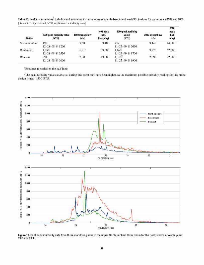
Table 10. Peak instantaneous1 turbidity and estimated instantaneous suspended-sediment load (SSL) values for water years 1999 and 2000 [cfs. cubic feet per second; NTU, nephelometric turbidity units]

2000 1999 peak 2000 peak turbidity peak

1999 peak turbidity value 1999 streamflow SSL value 2000 streamflow SSL Station (NTU) (cfs) (tons/day) (NTU) (cfs) (day)

North Santiam 198 7,580 9,400 739 9,140 44,000 12–28–98 @ 1200 11–25–99 @ 2030

Breitenbush 1,050 6,910 39,000 1,160 9,970 62,000 12–28–98 @ 0530 11–25–99 @ 1700

Blowout 891 2,800 19,000 1,3102 2,090 22,000 12–28–98 @ 0400 11–25–99 @ 1900

1Readings recorded on the half-hour.

2The peak turbidity values at Blowout during this event may have been higher, as the maximum possible turbidity reading for this probe design is near 1,300 NTU.

Figure 12. Continuous turbidity data from three monitoring sites in the upper North Santiam River Basin for the peak storms of water years 1999 and 2000.

29

Figure 13. Relation of measured to estimated suspended-sediment concentrations at three monitoring sites in the upper North Santiam River Basin, water years 1999 and 2000.

The fine material percentages were also plotted most of the annual SSL, all of the samples were greater
against streamflow and turbidity (not shown). The distributions and trends were similar to those in figure 17. This implies that, although correlations between turbidity and SSC used to estimate SSL are better than between streamflow and SSC, all three are correlated to the amount of larger diameter material in transit. That is, as SSC, streamflow, and turbidity increase, the larger particles represent a greater percentage of the SSL, principally due to higher stream velocities that keep heavier particles entrained in the water column. Conversely, the smaller particles are more prevalent throughout lower ranges of SSC, streamflow, and turbidity, especially at lower stream velocities, since the larger, heavier material has settled to the channel bottom, leaving only the smaller particles held in suspension.
The amount of sand that is part of the SSL can affect the relation between turbidity and SSC. Although sand particles are larger in diameter than silt or clay, the relative surface area of sand is smaller and will scatter less light than an equal weight of silt and clay. And, because sand particles are heavier than clays, they will settle out of suspension before silt and clay. Thus, when samples containing predominantly suspended clays are allowed to settle, they will have a higher turbidity than samples containing an equal weight of suspended sand. SSC data from the three sites indicates that for most of the daily SSLs, the predominant suspended particles were clays, although for higher SSCs (above 200 mg/l), which compose

than 80 percent particles coarser than clay. Because clay particles are the chief filtration problem for the Salem water treatment plant, and since most coarser material will settle in Detroit Lake or their respective channel bottoms, the sand component of the SSL is not considered a filtration problem, although the sand load will reduce the storage capacity of Detroit Lake.

Persistent-Turbidity Analysis

Turbidity-Decay Curves for the Annual Peak Streamflow Events

Figure 18 (p. 34) shows an example of how turbidity decays over time, from samples collected for the analysis of persistent turbidity during the largest streamflow and turbidity events of water years 1999 and 2000 at North Santiam, Breitenbush, and Blowout. A total of approximately 100 persistent-turbidity samples were collected at the 3 sites from October 1998 through September 2001. The two yearly peak samples shown in figure 18 illustrate differences in decay times between stations and storms. Two time scales are shown: the first depicting turbidity at up to 240 hours after settling, which spans the entire test period of 10 days (fig. 18A), and a second at a 12-hour time scale depicting persistent turbidity after 8.5 hours

30

Figure 14. Relation of measured to estimated suspended-sediment loads at three monitoring sites in the upper North Santiam River Basin, water years 1999 and 2000.

31

Figure 15. Statistical distribution of estimated mean daily suspended-sediment loads at three monitoring sites in the upper North Santiam River Basin, water years 1999 and 2000.

Figure 16. Estimated annual suspended-sediment yields at three monitoring sites in the upper North Santiam River Basin, water years 1999 and 2000.

(fig. 18B; see vertical bar representing the 0.002 mm clay particles). Turbidity persisted longer in water from Breitenbush and Blowout than from North Santiam for samples collected during the December 28–29, 1998, peak event (a 2- to 3-year recurrence interval flow event). Turbidity decayed by 75 and 86 percent after 8.5 hours from initial readings of 130 and 170 NTU in

Table 11. Estimated suspended-sediment loads and yields

Suspended-sediment loads

Estimated annual Estimated

suspended annual sediment suspended-

Station Water year

load (tons)

sediment yield (tons /mile2)

North Santiam 1999 16,500 76

2000 28,000 130

Breitenbush 1999 20,100 190

2000 51,000 470

Blowout 1999 15,000 570

2000 5,500 210

samples from Breitenbush and Blowout, respectively, as opposed to decaying by 94 percent from a starting turbidity of 50 NTU for the North Santiam sample. The residual turbidity value also remained high for both Breitenbush and Blowout, not dropping to below 10 NTU until the particles had settled for over 100 to 72 hours, respectively, well past the 8.5 hour persistent- turbidity criterion. (Turbidity values of 10 NTU and higher are considered a problem in the North Santiam River Basin, because it is difficult and expensive to reduce turbidity at this level in order to achieve the standard for drinking-water compliance.)

In the following year, samples collected during the November 25–26, 1999, peak event (a 10-year recurrence interval flow event; see table 4) at all three sites exhibited prolonged persistent turbidity, with levels dropping only between 73 to 82 percent after 8.5 hours of settling from initial turbidities ranging from 80 NTU at Blowout to 500 NTU at Breitenbush, respectively. Turbidity in the Blowout sample dropped below 10 NTU after 45 hours of settling time; values for Breitenbush and North Santiam remained above 10 NTU for at least 240 hours (10 days), at which time the test was halted.

In comparing the decay data between storms, the Blowout curves nearly overlay each other, differing only in their starting turbidity values, where as the North Santiam curves were significantly different, representing much higher persistent turbidity in 1999 than in 1998 (fig. 18). Breitenbush persistent turbidity was high for both storms.

These data represent persistent turbidity after only two storms, occurring a year apart. Data were not

32

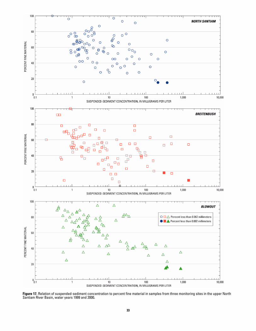
Figure 17. Relation of suspended-sediment concentration to percent fine material in samples from three monitoring sites in the upper North Santiam River Basin, water years 1999 and 2000.

33

Figure 18. Turbidity decay curves for samples collected during the peak storms of water years 1999 and 2000 at three monitoring sites in the upper North Santiam River Basin. Two time scales are shown for the same data. The vertical line in B represents the turbidity after a decay period of 8.5 hours. At this time, only clay-sized particles less than 0.002 millimeter would be in suspension.

necessarily collected concurrently or at the same time in the turbidity peak. And, as was noted in table 10, the instream peak turbidity value for the storms was also higher at Breitenbush and Blowout than at North Santiam for both years. Persistent-turbidity analysis in the entire study used at least 30 separate tests of persistent turbidity for each site, spread over 3 years and a range of flow conditions. Nonetheless, data from these two storms suggest that the higher the recurrence

interval of a storm, the longer high turbidity will persist in the upper North Santiam River Basin.

The storm data also illustrate the localized and multidimensional nature of sediment production in the major basins upstream of Detroit Lake. Persistent turbidity is highly variable and depends on multiple conditions, such as the intensity and duration of a storm and/or erosion event, amount of precipitation as either rain or snow, extent and depth of snowpack, landscape

34

exposure, geomorphic structure, terrain slope, and other climatic and geologic variables.

Analysis of Stream Persistent Turbidity

By using the linear regressions and equations relating initial sample turbidity to persistent turbidity (fig. 9, table 12), the 30-minute instream turbidity values for each site were converted to estimated persistent-turbidity values. This value represents the 0.002 mm diameter and smaller clay particles held in suspension, after the heavier, larger particles have settled out. The 30-minute persistent-turbidity values greater than or equal to 10 NTU were identified for each site.

Figure 19 shows the distribution of the 30-minute persistent-turbidity data. In water year 1999, Breitenbush had the highest median and mean persistent turbidity and largest interquartile (25th to 75th percentile) range in values. The 90th-percentile, at 45 NTU, was also the highest among the sites. The median, mean, and 90th percentile persistent-turbidity values at Blowout followed Breitenbush closely, although Blowout had over twice as many persistent turbidity values at or above 10 NTU as Breitenbush and over four times as many as North Santiam. North Santiam had the smallest 1999 median, mean, and 90th-percentile persistent-turbidity values.

In water year 2000, North Santiam had the highest median persistent-turbidity value at 42 NTU. The Breitenbush median was higher than in 1999, though lower than North Santiam’s, but Breitenbush had the highest mean value at 47 NTU. The Breitenbush 90th percentile was twice that of North Santiam. The 2000 Blowout values were similar to 1999 values. Blowout had over twice as many 30-minute persistent-turbidity values greater than or equal to 10 NTU than North Santiam, and slightly more than Breitenbush.

The 1999 and 2000 data exemplify the ubiquitous nature of fine clay material in the upper North Santiam River Basin, as no one subbasin generated markedly higher persistent-turbidity values than the others. Previous studies have documented the presence of clays throughout the upper basin, principally in large, deep-seated earthflows (Bates et al., 1998; Glassman, 1998). Fine clay material enters

the water column when the toe margins from these flows intercept streams and become eroded, mobilizing their clay content. The geology data also verify the widespread presence of clays in the upper basin. Figure 2 and table 2 both show the Breitenbush River and Blowout Creek subbasins as containing older, more erodible surficial geology with a higher clay content. In addition, landcover data has identified other potential sediment sources. Figure 3 and table 3 depict the Breitenbush River and upper North Santiam River subbasins as having more recently timber harvested land and open, alpine areas prone to higher sediment delivery to streams. More detailed landscape information is needed, particularly on soils and road density, to be more definitive about potential sediment and clay sources in these subbasins.

Turbidity-Decay Curves for Detroit Lake

Persistent-turbidity samples also were collected from three locations (Log Boom, Blowout, and Mongold) (fig. 20) in Detroit Lake on December 29, 1998, 1 day after the 1998 peak event. Samples were collected near the water surface and lake bottom, except for the Log Boom site, where the sample was collected only near the bottom, at a depth of 200 feet. Turbidity decay curves in figure 21A and figure 18 illustrate how turbidity persisted longer in the lake water than in stream water. All 8.5-hour readings, except Blowout-Surface were well above 10 NTU (fig. 21B). Also, the samples collected near the lake bottom had longer decay times than the samples collected at the surface. More study is needed in Detroit Lake to better understand turbidity fluctuations and retention times so as to better control downstream turbidity levels in water released through the lake outlet.

Clay-Water Volume Analysis

Because source water from the North Santiam River must be treated to remove suspended sediment and clays, it is important for treatment plant management to be able to predict the volume of water containing suspended clay (“clay water”) entering the system

35

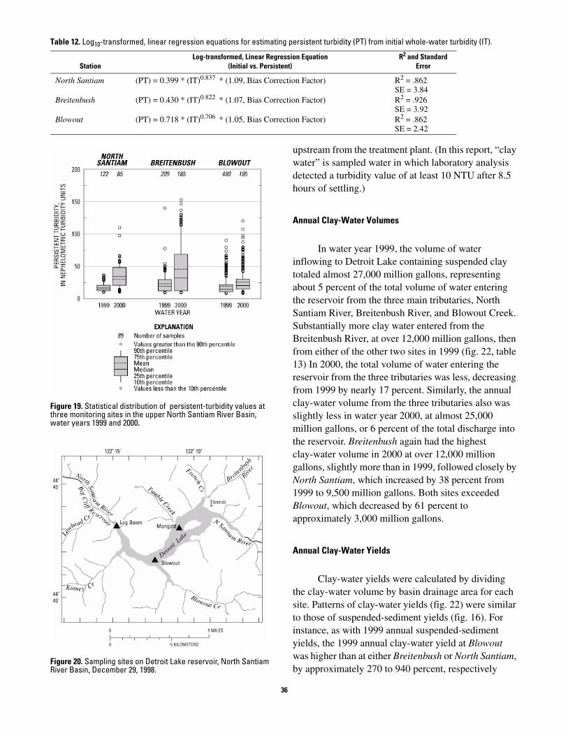
Table 12. Log10-transformed, linear regression equations for estimating persistent turbidity (PT) from initial whole-water turbidity (IT).

Log-transformed, Linear Regression Equation R2 and Standard Station (Initial vs. Persistent) Error

North Santiam (PT) = 0.399 * (IT)0.837 * (1.09, Bias Correction Factor) R2 = .862 SE = 3.84

Breitenbush (PT) = 0.430 * (IT)0.822 * (1.07, Bias Correction Factor) R2 = .926 SE = 3.92

Blowout (PT) = 0.718 * (IT)0.706 * (1.05, Bias Correction Factor) R2 = .862 SE = 2.42

Figure 19. Statistical distribution of persistent-turbidity values at three monitoring sites in the upper North Santiam River Basin, water years 1999 and 2000.

Figure 20. Sampling sites on Detroit Lake reservoir, North Santiam River Basin, December 29, 1998.

upstream from the treatment plant. (In this report, “clay water” is sampled water in which laboratory analysis detected a turbidity value of at least 10 NTU after 8.5 hours of settling.)

Annual Clay-Water Volumes

In water year 1999, the volume of water inflowing to Detroit Lake containing suspended clay totaled almost 27,000 million gallons, representing about 5 percent of the total volume of water entering the reservoir from the three main tributaries, North Santiam River, Breitenbush River, and Blowout Creek. Substantially more clay water entered from the Breitenbush River, at over 12,000 million gallons, then from either of the other two sites in 1999 (fig. 22, table 13) In 2000, the total volume of water entering the reservoir from the three tributaries was less, decreasing from 1999 by nearly 17 percent. Similarly, the annual clay-water volume from the three tributaries also was slightly less in water year 2000, at almost 25,000 million gallons, or 6 percent of the total discharge into the reservoir. Breitenbush again had the highest clay-water volume in 2000 at over 12,000 million gallons, slightly more than in 1999, followed closely by North Santiam, which increased by 38 percent from 1999 to 9,500 million gallons. Both sites exceeded Blowout, which decreased by 61 percent to approximately 3,000 million gallons.

Annual Clay-Water Yields

Clay-water yields were calculated by dividing the clay-water volume by basin drainage area for each site. Patterns of clay-water yields (fig. 22) were similar to those of suspended-sediment yields (fig. 16). For instance, as with 1999 annual suspended-sediment yields, the 1999 annual clay-water yield at Blowout was higher than at either Breitenbush or North Santiam, by approximately 270 to 940 percent, respectively

36

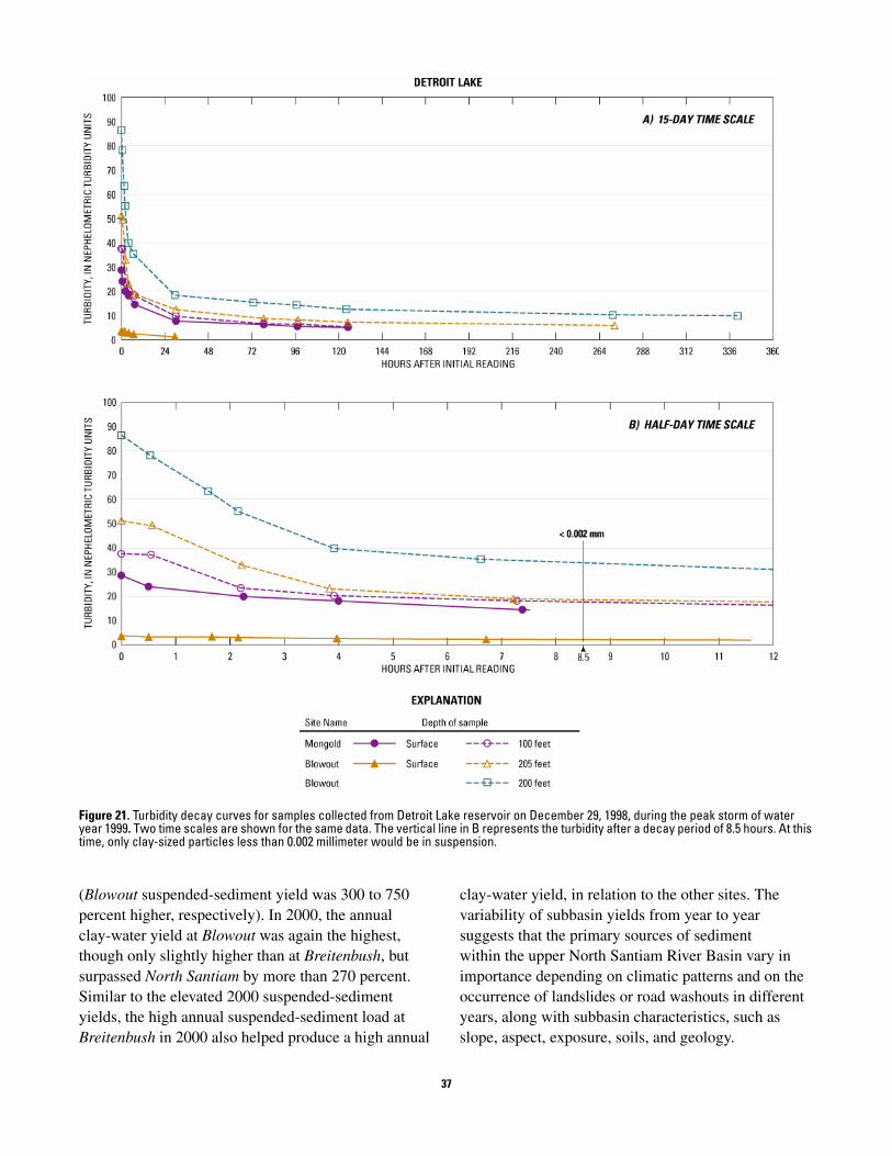
Figure 21. Turbidity decay curves for samples collected from Detroit Lake reservoir on December 29, 1998, during the peak storm of water year 1999. Two time scales are shown for the same data. The vertical line in B represents the turbidity after a decay period of 8.5 hours. At this time, only clay-sized particles less than 0.002 millimeter would be in suspension.

(Blowout suspended-sediment yield was 300 to 750 percent higher, respectively). In 2000, the annual clay-water yield at Blowout was again the highest, though only slightly higher than at Breitenbush, but surpassed North Santiam by more than 270 percent. Similar to the elevated 2000 suspended-sediment yields, the high annual suspended-sediment load at Breitenbush in 2000 also helped produce a high annual

clay-water yield, in relation to the other sites. The variability of subbasin yields from year to year suggests that the primary sources of sediment within the upper North Santiam River Basin vary in importance depending on climatic patterns and on the occurrence of landslides or road washouts in different years, along with subbasin characteristics, such as slope, aspect, exposure, soils, and geology.

37

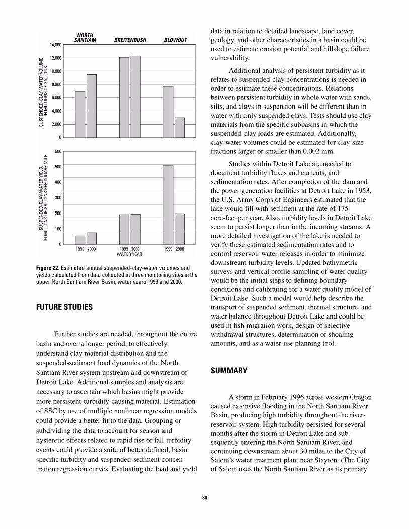
Figure 22. Estimated annual suspended-clay-water volumes and yields calculated from data collected at three monitoring sites in the upper North Santiam River Basin, water years 1999 and 2000.

FUTURE STUDIES

Further studies are needed, throughout the entire basin and over a longer period, to effectively understand clay material distribution and the suspended-sediment load dynamics of the North Santiam River system upstream and downstream of Detroit Lake. Additional samples and analysis are necessary to ascertain which basins might provide more persistent-turbidity-causing material. Estimation of SSC by use of multiple nonlinear regression models could provide a better fit to the data. Grouping or subdividing the data to account for season and hysteretic effects related to rapid rise or fall turbidity events could provide a suite of better defined, basin specific turbidity and suspended-sediment concentration regression curves. Evaluating the load and yield

data in relation to detailed landscape, land cover, geology, and other characteristics in a basin could be used to estimate erosion potential and hillslope failure vulnerability.

Additional analysis of persistent turbidity as it relates to suspended-clay concentrations is needed in order to estimate these concentrations. Relations between persistent turbidity in whole water with sands, silts, and clays in suspension will be different than in water with only suspended clays. Tests should use clay materials from the specific subbasins in which the suspended-clay loads are estimated. Additionally, clay-water volumes could be estimated for clay-size fractions larger or smaller than 0.002 mm.

Studies within Detroit Lake are needed to document turbidity fluxes and currents, and sedimentation rates. After completion of the dam and the power generation facilities at Detroit Lake in 1953, the U.S. Army Corps of Engineers estimated that the lake would fill with sediment at the rate of 175 acre-feet per year. Also, turbidity levels in Detroit Lake seem to persist longer than in the incoming streams. A more detailed investigation of the lake is needed to verify these estimated sedimentation rates and to control reservoir water releases in order to minimize downstream turbidity levels. Updated bathymetric surveys and vertical profile sampling of water quality would be the initial steps to defining boundary conditions and calibrating for a water quality model of Detroit Lake. Such a model would help describe the transport of suspended sediment, thermal structure, and water balance throughout Detroit Lake and could be used in fish migration work, design of selective withdrawal structures, determination of shoaling amounts, and as a water-use planning tool.

SUMMARY

A storm in February 1996 across western Oregon caused extensive flooding in the North Santiam River Basin, producing high turbidity throughout the river-reservoir system. High turbidity persisted for several months after the storm in Detroit Lake and subsequently entering the North Santiam River, and continuing downstream about 30 miles to the City of Salem’s water treatment plant near Stayton. (The City of Salem uses the North Santiam River as its primary

38

Table 13. Clay-water volumes and yields estimated from data collected at three monitoring sites in the upper North Santiam River Basin, water years 1999 and 2000

Estimated Estimated

Station Water year Annual discharge

(gallons x 106)

suspended-clay-water volume (gallons x 106)

Percent of annual discharge that is

suspended-clay water

suspended-clay-water yield

(gallons x 106 /mile2)

North Santiam 1999 315,000 6,900 2.2 32

2000 263,000 9,500 3.6 44

Breitenbush 1999 165,000 12,100 7.3 112

2000 140,000 12,300 8.8 114

Blowout 1999 38,200 7,700 20 296

2000 27,900 3,000 11 115

TOTAL for the three subbasins

1999

2000

518,000

431,000

26,600

24,700

5.2

5.8

76

71

drinking-water source). The treatment plant was unable to treat the turbid water with its slow-sand filtration system. Small clay materials (less than 0.002 mm) are responsible for the persistent turbidity and can pass through slow-sand water treatment filters. The water treatment facility was shut down for 8 days and water managers were forced to install more costly treatment methods and acquire water from neighboring water districts.

In 1998, the U.S. Geological Survey began a cooperative study with the City of Salem to investigate the sources and dynamics of turbidity within the North Santiam river-reservoir system. A real-time streamflow and water-quality monitoring network was installed, measuring continuous streamflow, water temperature, specific conductance, pH, and turbidity at three sites upstream of Detroit Lake. In April 2000, three sites were added downstream of Detroit Lake, with one additional site installed upstream of the lake in July 2001. An average of 90 samples analyzed for suspended-sediment concentration and percent of sediment finer than 0.062 mm were collected at sites near the mouths of the North Santiam River (as it enters Detroit Lake), Breitenbush River, and Blowout Creek from October 1998 to September 2001.

Two sets of linear regression correlations were developed to estimate suspended-sediment concentrations using (1) log-transformed discharge versus log-transformed suspended-sediment concentration and (2) log-transformed turbidity versus log-transformed suspended-sediment concentration. The suspended-sediment concentration data correlated better with turbidity than with discharge. In addition, peak turbidity events can skew the normal streamflow and

suspended-sediment relation by erosion of glacial and landslide deposits. Such events can affect the relationship of suspended-sediment production to streamflow, making streamflow unreliable for estimating suspended-sediment concentration (SSC). In addition, antecedent soil moisture conditions and differing time intervals between precipitation events affect sediment input to rivers, making turbidity more directly related to SSC and sediment delivery to streams than streamflow. Mean daily suspended- sediment loads were computed using the estimated suspended-sediment concentrations and streamflow for sites in the three subbasins (abbreviated North Santiam, Breitenbush, and Blowout) for October 1998 through September 2000.

Sand-silt fraction analysis indicated that as turbidity increased, the relative amount of fine material decreased. That is, at higher flows with higher turbidities, larger particles (sand) represented a greater portion of the total suspended-sediment load. The amount of larger particles relative to smaller particles can significantly alter the turbidity-SSC relation.

The instream (whole water) turbidity values were converted to an estimated persistent (residual) turbidity value by a third linear regression. The persistent- turbidity value was estimated using turbidity decay curves and settling times determined from Stokes law for 0.002 mm diameter clay particles after 8.5 hours of settling. An analysis of the persistent-turbidity data was completed for the three upper sites and Detroit Lake. Blowout and Breitenbush had higher values of persistent turbidity at greater than or equal to 10 NTU than North Santiam. (Source water having turbidity greater than 10 NTU must be pretreated prior to normal

39

processing at the City of Salem’s water treatment plant.).

Volumes of water containing suspended clay entering Detroit Lake from the three subbasins were estimated using the three estimated persistent turbidity values and their corresponding streamflow. Volumes of water containing suspended clay at 10 NTU and higher (“clay water”) were calculated from the persistent-turbidity laboratory tests. Breitenbush had the highest annual clay-water volume for water years 1999 and 2000.

High rainfall events in the North Santiam River Basin cause most of the annual suspended-sediment loads. To adequately determine annual suspended- sediment loads using turbidity as a surrogate, samples should be collected over the entire annual hydrograph, and especially during peak streamflow events. The peak storms for 1999 and 2000 were each responsible for about two-thirds of the annual suspended-sediment load entering Detroit Lake from the North Santiam River, Breitenbush River, and Blowout Creek. Both storms were 3-day events and represented the 2- to 3-year recurrence interval in 1999 and the 10-year recurrence interval in 2000. Storm events with larger yearly recurrence intervals will probably generate higher turbidities that will persist longer in the upper basin streams.

Geology data showed that the smaller basins of Breitenbush River and Blowout Creek had higher percentages of older, defined soils, and hydrothermally altered, erodible sedimentary, basaltic, andesitic, and other volcaniclastic rocks, along with highly mobilized glacial or landslide deposits. These materials contain smectite and other clay particles that cause persistent turbidity. North Santiam was composed mostly of younger, less erodible basalts and andesites containing fewer clays, with some glacial deposits. Land-cover data identify the Breitenbush and North Santiam subbasins as containing more recently harvested timber lands, with a greater percentage of open, alpine communities, which could be more erodible during intense precipitation events.

The water year 1999 and 2000 yield data suggests that Breitenbush River and Blowout Creek contribute more suspended sediment and clay water per unit area than the upper North Santiam River. Also, the percentage of clay as part of the total annual water volume was higher for Blowout Creek and Breitenbush River than for the upper North Santiam River for both years of data. The total volume of water entering Detroit Lake from the three streams for both years

averaged about 5 percent suspended-clay water. Higher annual suspended-sediment and clay-water yields were observed from the smaller basins, indicating that basin characteristics might play a more important role in determining sediment production than in larger basins. Such yields could be used to identify possible sediment sources. Lastly, correlations developed between turbidity and suspended-sediment concentration data are basin specific and can change within a single basin from year to year. Climatic, landslide, and glacial events and conditions in the North Santiam River Basin will affect these relations.

REFERENCES CITED

Ambers, R.K.R., 1998, Effects of land use on the concentration and clay mineralogy of suspended sediments in streams of the Dorena Lake Watershed, Western Oregon, American Geophysical Union, Abstracts for 1998 Fall Meeting, San Francisco, California: http:// earth.agu.org/meetings/ waisfm98.hml, accessed March 1, 2001.

Austin, R.W., 1973, Problems in measuring turbidity as a water quality parameter: Seminar on Methodology for Monitoring the Marine Environment: Seattle, Washington, 11 p.

Bates, D., Willis, K., Swanson, F., Glasmann, J. R., Halemeier, D., Wujcik, H., 1998, North Santiam River turbidity study, 1996–1997: Berkeley, University of California, Watershed Management Council Networker, p. 1–17.

Beschta, R.L., 1980, Turbidity and suspended sediment relationships, in Proceedings of Watershed Management Symposium, Irrigation and Drainage Division, American Society of Civil Engineers, Boise, Idaho, July 21–23, 1980: p. 271–282.

Bilby, R.E., 1985, Contributions of road surface sediment to a Western Washington stream: Forest Science: v. 31, no. 4, p. 827–838

Brabben, T.E., 1981, Use of turbidity monitors to access sediment yield in East Java, Indonesia: Proceedings of the IAHS Florence Symposium, June 22–26, 1981, Publication No. 133, p. 105–113.

Christensen, V.G., Xiaodong, J., Ziegler, A.C., 2000, Regression analysis and real-time water-quality monitoring to estimate constituent concentrations, loads, and yields in the Little Arkansas River, South-Central Kansas, 1995–99: U.S. Geological Survey Water-Resources Investigations Report 00–4126, 36 p.

Cohn, T.A., Caudler, D.L., Gilroy, E.J., Zynjuk, L.D., Summers, R.M., 1992, The validity of a simple statistical model for estimating fluvial constituent

40

loads; an empirical study involving nutrient loads entering Chesapeake Bay: Water Resources Research, v. 28, no. 9, p. 2353–2363.

Colby, B.R., 1963, Fluvial sediments—A summary of source, transportation, deposition, and measurement of sediment discharge: U.S. Geological Survey Bulletin 1181–A, 47 p.

Costa, J.E., 1977, Sediment concentration and duration in stream channels: Journal of Soil and Water Conservation, v. 32, p. 168–170.

Cotton, C.S., Dominicci, A.J., Feldman, D.S., Pilatzke, C.L., 1998, Oregon Watersheds—Many activities contribute to increased turbidity during large storms: Washington, D.C., U.S. Government Accounting Office GAO/ RCED–98–220, 69 p.

Curtiss, D.A., 1982, An evaluation of suspended sediment and turbidity in Cow Creek, Oregon: U.S. Geological Survey Open-File Report 82–364, 21 p.

Davies-Colley, R.J., Smith, D.G., 2001, Turbidity, suspended-sediment, and water clarity—A review: Journal of the American Water Resources Association, v. 37, no. 5, p. 1085–1101.

Edwards, T.K., Glysson, G.D., 1999, Field methods for measurement of fluvial sediment: Techniques of Water-Resources Investigations of the U.S. Geological Survey, Book 3, Chapter C2, 89 p.

Ewing, R., Mohrman, J., 1989, Suspended sediment and turbidity from Northern Yellowstone Park, Wyoming, 1985–1987: Bethesda, Maryland, Proceeding of the Symposium on Headwaters Hydrology, American Water Resources Association, p. 213–222.

Ferguson, R.I., 1986, River loads underestimated by rating curves: Water Resources Research, v. 22, no. 1, p. 74–76.

Gippel, C.J., 1989, Use of turbidimeters in suspended sediment research: Hydrobiologia, v. 176, no. 17, p. 465–480.

Glasmann, J.R., 1998, Soil erosion and water quality in the Western Cascades, Oregon: Baltimore, Maryland, Willamette Geological Services, Annual Meeting Abstracts, American Society of Agronomy, Crop Science Society of America, and Soil Science Society of America, October 18–22, 1998, p. 344.

Guy, H.P., 1969, Laboratory theory and methods for sediment analysis: U.S. Geological Survey Techniques of Water-Resources Investigations, Book 5, Chapter C1, 58 p.

Guy, H.P., 1970, Fluvial Sediment Concepts: U.S. Geological Survey Techniques of Water-Resources Investigations, Book 3, Chapter C1, 52 p.

Harr, R.D., 1986, Effects of clearcutting on rain-on-snow runoff in Western Oregon—A new look at old studies: Water Resources Research, v. 22, no. 7, p. 1095–1100.

Harr, R.D., Harper, W.C., Krygier, J.T., and Hsieth, F.S., 1975, Changes in storm hydrographs after road building

and clear-cutting in the Oregon Coast Range: Water Resources Research, v. 11, no. 3, p. 436–444.

Harris, D.D., 1977, Hydrologic changes after logging in two small Oregon Coastal Watersheds: U.S. Geological Survey Water-Supply Paper 2037, 31 p.

Helsel D.R., Hirsh R.M., 1992, Statistical methods in water resources: New York, Elsevier, 522 p.

Herrett, T.A., House, J.G., Ruppert, G.P., Courts, M.L., 2000, Water resources data, Oregon, Water Year 2000: U.S. Geological Survey Water-Data Report OR–00–1, 493 p.

Hyams, D.C., no date, CurveExpert 1.34—A comprehensive curvefitting system for Windows: http:// www.ebicom.net/~dhyams/cvxpt.htm, accessed March 13, 2003.

Ingebritsen, S.E., Mariner, R.H., Sherrod, D.R., 1991, Hydrothermal systems of the Cascade Range, north-central Oregon: U.S. Geological Survey Open File Report 91–69, 217 p.

Kagan, J., Caicco, S., 1992, Manual of Oregon actual vegetation, Oregon Gap Analysis Program: Portland, Oregon, U.S. Fish and Wildlife Service, 180 p.

Koeppen, J., 1974, Turbidity measurement–An overview, in Proceedings of Turbidity Workshop, U.S. National Oceanic Instrumentation Center, Washington, D.C., May 6–8: p. 11–12.

Kunkle, S.H., Comer, G.H., 1971, Estimating suspended sediment concentrations in streams by turbidity measurements: Journal of Soil and Water Conservation, v. 36, p. 18–20.

Laenen, A., Hansen, P.R., 1985, Preliminary study of the water-temperature regime of the North Santiam River downstream from Detroit and Big Cliff Dams, Oregon: U.S. Geological Survey Water-ResourcesInvestigations Report 84–4105, 45 p.

LaHuzen, R.G., 1994, Variations in turbidity in streams of the Bull Run watershed, Oregon, Water Years 1989–90: U.S. Geological Survey Water-ResourcesInvestigations Report 93–4045, 28 p.

Loper, C.A., Wetzel, K.L., 1988, Sediment loads, discharges, and yields in the East Branch Mahoning Creek Basin, Clearfield and Jefferson Counties, Pennsylvania, June 1979 through September 1981: U.S. Geological Survey Water-Resources Investigations Report 85–4213, 26 p.

Major, J.J., Pierson, T.C., Dinehart, R.L., Costa, J.E., 2000, Sediment yield following severe volcanic disturbance- A two-decade perspective from Mount St. Helens: Geology, v. 28, no. 9, p. 819–822.

Omernick, J.M., Gallant, A.L., 1986, Ecoregions of the Pacific Northwest: U.S. Environmental Protection Agency report EPA 600/3–86/033, 39 p.

Oregon Administrative Rules (OAR), 2000, Chapter 340— Department of Environmental Quality, Division 41—

41

Water Pollution, Section 445—Willamette River Basin (2)(c), v. 5, p. 584.

Oregon Administrative Rules (OAR), 2001, Chapter 333— Department of Human Services, Oregon Health Division, Division 61—Public Water Systems, Section 30:—Maximum Contaminant Levels and Action Levels (3) (B) (i) (ii), p. 20.

Oregon Climate Service, Oregon annual precipitation map 1961–1990: http://www.ocs.orst.edu/prism, accessed February 5, 2001.

Oregon Department of Environmental Quality, 2000, Umatilla River Basin TMDL and WQMP: http:// waterquality.deq.state.or.us/wq/TMDLs/TMDLs.htm, accessed March 1, 2001.

Paustian, S.J., Beschta, R.L., 1979, The suspended sediment regime of an Oregon Coast Range stream: Water Resources Bulletin, v. 15, p. 144–154.

Pearch, J.M., 2000, Relationships between landscape stability, clay minerology, and stream turbidity in the South Santiam Watershed, Western Cascades, Oregon: Corvallis, Oregon State University, M.S. Thesis, 199 p.

Peck, D.L., Griggs, A.B., Schlicker, H.G., Wells, F.G., Dole, H.M., 1964, Geology of the central and northern parts of the Western Cascade Range in Oregon: U.S. Geological Survey Professional Paper 449, 56 p.

Pickering, R.J., 1976, Measurement of “turbidity” and related characteristics of natural waters: U.S. Geological Survey Open-File Report 76–153, 13 p.

Porterfield, G., 1972, Computations of fluvial-sediment discharge: Techniques of Water-Resources Investigations of the U.S. Geological Survey, Book 3, Chapter C3, 66 p.

Rainwater, F.H., Thatcher, L.L., 1960, Methods for collection and analysis of water samples: U.S. Geological Survey Water-Supply Paper 1454, p. 301

Rantz, S.E. and others, 1982, Measurement and computation of streamflow: U.S. Geological Survey, Water-Supply Paper 2175, 2 Volumes, 631 p.

Reid, L.M., and Dunne, T., 1984, Sediment production from forest road surfaces: Water Resources Research, v. 20, no. 11, p. 1753–1761.

Rinella, J.F., McKenzie, S.W., 1982, Method for relating suspended-sediment concentrations to suspended- sediment particle-size classes in storm-water runoff: U.S. Geological Survey Water-Resources Investigation Report 82–39, 43 p.

Ruffing, F.E., Britton, J.L., Flint, N.A., 1997, Effect of the February flood on the City of Salem water supply, in The Pacific Northwest Floods of February 6–11, 1996—Proceedings of the Pacific Northwest Water Issues Conference, Portland, Oregon, October 7–8, 1997: American Institute of Hydrology, p. 31–37.

Sadar, M., 1996, Understanding turbidity science: Loveland, Colorado, Hach Co., Technical Information Series- Booklet no. 11, 24 p.

Sadar, M., 1997, Turbidity Standards: Loveland, Colorado, Hach Co., Technical Information Series-Booklet no. 12, 14 p.

Salem, City of, 1999, Annual report of Salem’s drinking water, Volume 2: Salem, Oregon, Public Works Department, 8 p.

Sherrod, D.R., Ingebritsen, S.E., Curless, J.M., Keith, T.E., Diaz, N.M., DeRoo, T.G., Hurlocker, S.L., 1996, Water, rocks, and woods—A field excursion to examine the geology, hydrology, and geothermal resources in the Clackamas, North Santiam, and McKenzie River drainages, Cascade Range, Oregon: Oregon Geology, v. 58, no. 5, p. 103–124.

Sidle, R.C. and Campbell, A.J., 1985, Patterns of suspended sediment transport in a coastal Alaska stream: Water Resources Bulletin WARBAQ v. 21/6, p. 909–917.

Swanson, F.J., Dryness, C.T., 1975, Impact of clear-cutting and road construction on soil erosion by landslides in the western Cascade Range, Oregon: Geology, v. 3, no. 7, p. 393–396.

Taskey, R.D., 1978, Relationships of clay minerology to landscape stability in Western Oregon: Corvallis, Oregon State University, PhD Dissertation, p. 223.

Truhlar, J.R., 1976, Determining suspended sediment loads from turbidity records, in Proceedings of the Third Inter-Agency Sedimentation Conference, Water Resources Council, Denver, Colorado: p. 65–74.

U.S. Army Corps of Engineers, 1953, Detroit Lake Water Control Manual, Detroit Dam Project: p. 33–34.

U.S. Environmental Protection Agency, 1996, Level III ecoregions to the continental United States (revision of Omernick, 1987): Corvallis, Oregon, U.S. Environmental Protection Agency-National Helath and Environmental Effects Research Laboratory Map M-1, various scales.

U.S. Environmental Protection Agency, 2000, Ambient water quality criteria recommendations, rivers and streams in nutrient Ecoregion II: EPA 822–B–00–015, 120 p.

U.S. Geological Survey, 1990, Land use and land cover digital data from 1:250,000- and 1:100,000-scale maps—Data user guide 4: Reston, Virginia, 25 p.

Vanoni, Vito A. (ed.), 1975, Sedimentation Engineering: New York, American Society of Civil Engineers, 743 p.

Wagner, R.J., Mattraw, H.C., Ritz, G.F., Smith, B.A., 2000, Guidelines and standard procedures for continuous water-quality monitors—Site selection, field operation, calibration, record computation, and reporting: U.S. Geological Survey Water-Resources Investigation Report 00–4252, 53 p.

Walder, J.S., and Driedger, C.L., 1994, Rapid geomorphic change caused by glacial outburst floods and debris floods along Tahoma Creek, Mount Rainier, Washington, U.S.A.: Arctic and Alpine Research, v. 26, n., 4, p. 319–327.

42

Walder, J.S. and Driedger, C.L., 1995, Frequent outburst floods from South Tahoma Glacier, Mount Rainier, U.S.A.—Relation to debris flows, meteorological origin and implications for subglacial hydrology: Journal of Glaciology, v. 41, no. 137: 1, 10 p.

Walker, G.W. and MacLeod, N.S., 1991, Geologic map of Oregon: U.S. Geological Survey, 2 sheets, scale 1:500,000.

Wellman, R.E., Gordon, J.M., Moffatt, R.L., 1993, Statistical summaries of streamflow data in Oregon,

Volume 2—Annual low and high flow, and instantaneous peak flow: U.S. Geological Survey Open-File Report 93–63, 406 p.

Youngberg, C.T., Harvard, M.E., Simonson, G.H., Rai, D., Klingeman, P.C., Larson, D.W., Phinney, H.K., Bell, J.R., 1971, Hills Creek Reservoir Turbidity Study: Corvallis, Oregon State University, Water Resources Research Institute, p. 252.

43

Back Cover Photographs:

Top left: Datasonde pipe, outside staff, and crest-stage gage at French station.

Top right: Sampling turbid water from Breitenbush station cableway.

Bottom left: Turbid water entering the North Santiam River from Little Sardine Creek, just upstream of Niagara station.

Bottom right: Muddy plume entering Detroit Lake from Breitenbush River after high-turbidity event.

looking upstream from breitenbush - usgs · looking upstream from breitenbush station during high...

Documents