loop closing in slam - technical university of denmarketd.dtu.dk/thesis/271982/bac10_43_net.pdf ·...
TRANSCRIPT

Loop Closing in SLAM
Kinna Majvig Knudsen
Kongens Lyngby 2010IMM-B.Sc-2010-43

Technical University of DenmarkInformatics and Mathematical ModellingBuilding 321, DK-2800 Kongens Lyngby, DenmarkPhone +45 45253351, Fax +45 [email protected]
IMM-B.Sc: ISSN 0909-3192

Summary
A general problem in the navigation system of mobile robots is the integrationerror, which will cause the robot’s location to be very inaccurate at some point.The loop closing procedure detects previously visited places which is used toadjust the positions, and thus reduce the effect of the error. This thesis isexamining a visual approach of detecting the presence of a loop. Here, images areused to represent places and the SIFT algorithm is used to extract informationfrom these images. A database of previously visited places is created from thisinformation, where each place is represented as in the Bag-of-Words model ina visual version. The structure of the database is created as a vocabulary tree.The partition of known and unknown places is based on a statistical approach.Altogether the system received a 44% final recognition rate at its maximumperformance whereas the recognition rate for the image detection alone was91%.This shows that the visual approach is useful, but the system would still needsome improvements before it can be used as a robust tool for loop detection.

ii

Resume
Et generelt problem i navigationen for mobile robotter er den integrerede fejl,som forarsager at lokaliseringen af robotten bliver meget upræcis pa et tid-spunkt. Løkke luknings proceduren opdager hvis robotten befinder sig pa ettidligere besøgt sted, og dette bruges til at justere positionerne, og deraf reduc-ere effekten af fejlen. Denne rapport undersøger en visuel tilgang til at opdagetilstedeværelsen af en løkke. Her er billeder brugt til at repræsentere stederne ogSIFT algoritmen er brugt til at hente information i disse billeder. En databaseaf tidligere besøgte steder er fremstillet af disse informationer, hvor hvert steder repræsenteret som i Bag- of-Words modellen i en visuel version. Strukturenaf databasen er fremstillet som et ord-træ. Adskillelsen af kendte og ukendtesteder er baseret pa en statistisk fremgangsmade. Tilsammen opnaede systemeten 44% genkendelsesrate ved den maksimale ydeevne, hvor genkendelsesratenfor billedgenkendelsen alene var 91%. Dette viser at en visuel fremgangsmadeer brugbar, men at systemet har brug for nogle forbedringer før det kan brugessom et robust værktøj til løkke genkendelse.

iv

Preface
This thesis was prepared at Informatics Mathematical Modelling, the TechnicalUniversity of Denmark in partial fulfillment of the requirements for acquiring abachelor degree in engineering.
The thesis deals with the problem of detecting the presence of a loop in the loopclosing problem in SLAM.
Lyngby, December 2010
Kinna Majvig Knudsen

vi

Acknowledgements
First I would like to thank my supervisor Henrik Aanæs for inspiration andguidance in this project.Also Anders Lindbjerg Dahl, Line Katrine Harder Clemmensen and RasmusLarsen has been a great help during the period with weekly guidance and Iwould like to thank them as well.At last I would like to thank Nancy Pietropaolo and Lukas Roy Svane Theisenfor a very helpful proofreading of the report.

viii

Contents
Summary i
Resume iii
Preface v
Acknowledgements vii
1 Introduction 1
1.1 Background . . . . . . . . . . . . . . . . . . . . . . . . . . . . . . 1
1.2 The problem . . . . . . . . . . . . . . . . . . . . . . . . . . . . . 4
1.3 Related Work . . . . . . . . . . . . . . . . . . . . . . . . . . . . . 4
1.4 Thesis Structure . . . . . . . . . . . . . . . . . . . . . . . . . . . 5
2 Theory and Implementation 7
2.1 The SIFT Algorithm . . . . . . . . . . . . . . . . . . . . . . . . . 7
2.2 The Vocabulary Tree . . . . . . . . . . . . . . . . . . . . . . . . . 12
2.3 Comparing Images . . . . . . . . . . . . . . . . . . . . . . . . . . 17
2.4 The Match Detector . . . . . . . . . . . . . . . . . . . . . . . . . 19
3 Tests and Results 23
3.1 The Datasets . . . . . . . . . . . . . . . . . . . . . . . . . . . . . 24
3.2 General Performance and Significance of the Vocabulary Size . . 26
3.3 Performance of the Match Detector . . . . . . . . . . . . . . . . . 29
3.4 Performance of the Match Detector with Positions Added . . . . 31
3.5 Unsuccessful Tests . . . . . . . . . . . . . . . . . . . . . . . . . . 33

x CONTENTS
4 Discussion 354.1 The General Recognition System . . . . . . . . . . . . . . . . . . 354.2 The Match Detector . . . . . . . . . . . . . . . . . . . . . . . . . 364.3 The Overall System . . . . . . . . . . . . . . . . . . . . . . . . . 374.4 Future Work . . . . . . . . . . . . . . . . . . . . . . . . . . . . . 38
5 Conclusion 41
A Mathematical Review 43A.1 The Hessian Matrix . . . . . . . . . . . . . . . . . . . . . . . . . 43
B Datasets 45B.1 Dataset 1 . . . . . . . . . . . . . . . . . . . . . . . . . . . . . . . 46B.2 Dataset 2 . . . . . . . . . . . . . . . . . . . . . . . . . . . . . . . 48B.3 Dataset 3 . . . . . . . . . . . . . . . . . . . . . . . . . . . . . . . 49B.4 Dataset 4 . . . . . . . . . . . . . . . . . . . . . . . . . . . . . . . 51
C Testresults 53
D Running the Software 55

Chapter 1
Introduction
This chapter gives an introduction to the project dealing with loop closing inSLAM. Both loop closing and SLAM is introduced and explained together withsome general information of the topic of robotics where these are relevant. Also,the problem that this thesis is going to solve is introduced and defined.
1.1 Background
For a mobile robot, navigation is an essential ability. Depending on the typeof robot, different navigation methods exist, from being manually controlledby a driver either on the robot or from a distance, using sensors to followlines or the robot being able to ”see” the environment and localize its position.The last example is referred to as an autonomous robot, it needs no humaninteraction. Such navigation ability is used in robots for planetary exploration,subsea vehicles, air-borne vehicles and vehicles for tasks such as mining andconstruction. This is also the kind of robot navigation that has no generalsolution. However, in the last decade, working methods have arisen by usingthe SLAM approach.

2 Introduction
Figure 1.1: NASA’s Mars Exploration Rover Opportunity on the surface of Marsin an artist’s edition. Such a robot needs a high degree of autonomous abilitiesas no external help in navigation is possible. The image is taken from NASA’swebsite.
1.1.1 SLAM
SLAM stands for Simultaneous Localization and Mapping and is the process ofwhich a robot builds a map of its environment while at the same time determinesits location in that environment. Many methods have been used to solve thisproblem, and SLAM has been implemented in a number of different domainsranging from indoor and outdoor robots to underwater and airborne systems.The methods existing today allows the problem to be considered as solved, butsome issues remain for the robot to be truly autonomous.[3]
1.1.2 Loop Closing
A simple approach for a robot to determine its position is by using odometry,which estimates the current position based on a start position. Data from therobot’s actuators is used to calculate movements, for example for a wheel itwould be the wheel’s circumference and how many times the wheel has turned.Then to avoid collisions the robot could use sensors. The big problem in thismethod is the integrating error in the odometry, no matter how precisely andwell-calibrated the system is, a small error is inevitable. And the further therobot moves, the more the error enlarges. Imagine a robot supposed to move ina quadrangle as shown in Figure 1.2, if the straight line is a little off, the robotwill not end up where it thinks it will end up.The solution to this problem is referred to as closing the loop. If the robot couldsomehow recognize a place from an earlier visit, it would be able to comparethe calculated positions and adjust any errors that have occurred. This is acommon challenge in the SLAM problem. While the robot is moving around, it

1.1 Background 3
gathers information about its environment and groups it into one of the followingcategories: unknown environment, known environment or no decision about theenvironment. If it decides that the environment is unknown, information aboutthis place is stored in a database. Comparative to other mapping processes,storing images in the database is a simpler approach. If it decides that theenvironment is already known, this can be used to redetermine the presentlocation of the robot. This condition takes care of inaccurate positions causedby the integrating error.[11]
Figure 1.2: A robot supposed to move in a quadrangle indicated by the dottedline. A small error will grow as the robot moves further, and the robot will notend up where it is supposed to.
1.1.3 Image Analysis
Most humans have the ability to recognize a place, and all we use is our eyes,memory and some rational logic. So providing a robot with a camera andsome memory, it should have the same prerequisites as humans. The systemimplemented in the robot is representing the logic.However, some corrections need to be done. First of all, the image from thecamera will be nothing but a matrix with pixel values which does not say muchabout the actual content in the image. By analysing an image, or matrix ofpixel values, it is possible to extract more meaningful information about theimage, and this information can be stored as the memory of a place.

4 Introduction
1.2 The problem
Motivation
The challenge in the process of closing a loop is to first detect that a loop ispresent. A method to do this is providing the robot with a camera and let animage from each visited position represent that position. Here, the plane imagewould not make a good representation for a place. However, by analyzing theimage and extracting descriptive information, the image might turn out to bevery representative. The problem of detecting a loop has now turned into theproblem of finding a matching image, which makes a more concrete predicament.
Goal
The goal for this project is to implement a system able to recognize a previouslyvisited place, using images to represent the places.The SIFT algorithm will be used to extract information about the images, andthe task is then an implementation of a system to compare this informationabout the images and distinguish between known images and unknown images.The comparison of images is based on the Bag-of-Words model, which is usedin text search engines, here converted to the use of images.
Delimitations
The project will look at the recognition part only, and will not go further intothe loop closing procedure once a place is recognized.To extract information in the images an algorithm called the SIFT algorithmwill be used, without any improvements such as adding color information. Also,the process of building and searching in the database is based on a tree structure,and other possible ways of doing this will not be taken into account.
1.3 Related Work
The topic of loop closing and SLAM is not new. Many researchers have beenworking with this for years, and as a result many systems have been developed

1.4 Thesis Structure 5
to solve the problem of an open loop in SLAM.Using a visual approach to separate the loop detector from the primary nav-igation tool, is not new either. Newman and Ho[11, 12] have made a systemto close a loop using visual features as input together with data from scanninglasers to draw the map. Their system made it possible for the robot to detectthe presence of a loop and adjust the position. Their approach did also useSIFT descriptors to extract image information and an inverted file to search forsimilar images.The use of a vocabulary tree was introduced by Nister and Stewenius [13] withthe goal to make searching in larger databases faster. The vocabulary tree haslater on been implemented in the searching process for loop closing by Callmerand Granstrom [2], who also made a system that could detect and close a loop.Here, a different image feature extractor than SIFT was used.
1.4 Thesis Structure
The fundamentals of this thesis are broken into two large parts. The first partis the Theory and Implementation in chapter 2, which gives a basic insight inthe two algorithms used in the process of making the system able to recognizea place. It also describes additional concepts and methods that the system isusing, and how these are implemented.The second part is the Tests and Results in chapter 3, which describes the com-pleted tests and the results that shows that the system really does work.In chapter 4, a discussion of the results and the system in general can be found.Both cases where the system can be used to detect a previously visited placeand where it cannot, will be discussed. Lastly, this is all summed up in a conciseconclusion in chapter 5.

6 Introduction

Chapter 2
Theory and Implementation
In this chapter, all the theory used to implement the image recognition systemis explained. The basis to make an image recognizable is to extract descriptorsfrom it, and here the SIFT algorithm is used. A detailed description of how thisalgorithm works is found in the first section. Furthermore, the structure of thedatabase is described together with the method to compare images. At last, thetheory behind the match detector and the way it is implemented are presented.
2.1 The SIFT Algorithm
The Scale Invariant Feature Transform (SIFT) algorithm is developed by DavidLowe and is patented in the US. The patent makes it available to research useonly, and it can be found on David Lowe’s website [10]. The algorithm is, asthe name reveals, invariant to the scale of the object and also rotations. Fur-thermore, it is partially invariant to 3D-viewpoint and illumination.[9]
The SIFT-algorithm operates in these four steps which will be described indetail in the next four sections:
8 Theory and Implementation
1. Scale space extrema detection2. Keypoint localization3. Orientation assignment4. Keypoint descriptor
2.1.1 Scale Space Extrema Detection
The first step is to detect scale space extrema, which will be the first set ofkeypoints. The scale space of an image is defined as
L(x, y, σ) = G(x, y, σ) ∗ I(x, y), (2.1)
G(x, y, σ) =1
2πσ2e−(x
2+y2)/2σ2
(2.2)
where G(x, y, σ) is the Gaussian function or filter, I(x, y) is the image and σ isthe scale.To detect stable keypoints, Lowe is using scale space extrema in the difference-of-Gaussian function convolved with the image
D(x, y, σ) = (G(x, y, kσ)−G(x, y, σ)) ∗ I(x, y)
= L(x, y, kσ)− L(x, y, σ). (2.3)
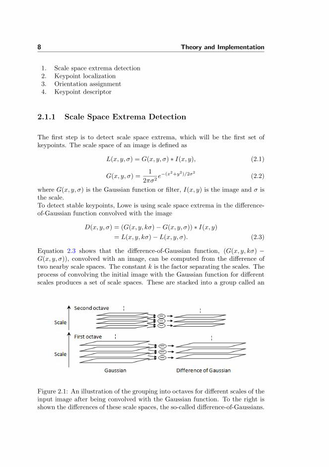
Equation 2.3 shows that the difference-of-Gaussian function, (G(x, y, kσ) −G(x, y, σ)), convolved with an image, can be computed from the difference oftwo nearby scale spaces. The constant k is the factor separating the scales. Theprocess of convolving the initial image with the Gaussian function for differentscales produces a set of scale spaces. These are stacked into a group called an
Figure 2.1: An illustration of the grouping into octaves for different scales of theinput image after being convolved with the Gaussian function. To the right isshown the differences of these scale spaces, the so-called difference-of-Gaussians.

2.1 The SIFT Algorithm 9
Figure 2.2: The local extrema (marked in black) is compared to its 26 neighbors(marked in grey), 8 in the same scale and 9 for both the scale below and thescale above.
octave. After this, the image is reduced in size by a factor of 2 and the sameprocess is carried out to create a second octave, then a third and so on. Figure2.1 illustrates this approach. The last two images in the octave are used toresample the Gaussian image for this octave by taking every second pixel ineach row and column. Now to detect the local extrema, each pixel is comparedto its 26 neighbors, 8 in the same scale, and 9 for both the scale below and thescale above. If the pixel is either larger or smaller than all the neighbors, it isselected as a keypoint. This is illustrated in Figure 2.2.
2.1.2 Keypoint Localization
The second step is to discard points which have low contrast or are poorly local-ized along an edge. Here the Taylor expansion up to the quadratic term is usedto determine an interpolated location of the keypoint. The Taylor expansion ofthe scale space function is shifted so that the origin is at that keypoint.
D(x) = D +∂DT
∂xx +
1
2xT
∂2D
∂x2x, (2.4)
where x = (x, y, σ)T is the offset from the keypoint and D and the derivativesof D are the difference-of-Gaussian function evaluated at the keypoint. Thelocation of the keypoint or extremum x is now found by taking the derivativeof this function with respect to x and setting it to zero:
x =∂2D−1
∂x2
∂D
∂x. (2.5)
Inserting equation 2.5 into equation 2.4 will give the interpolated estimate ofthe location of the extremum:
D(x) = D +1
2
∂DT
∂xx. (2.6)

10 Theory and Implementation
Keypoints with low contrast will be poorly localized, so discarding all extremawith |D(x)| smaller than some threshold will remove these points from the set.Still there will be poorly localized keypoints along edges, because these edgesgive off a high response in the difference-of-Gaussian function. However thedifference-of-Gaussian will have a large principal curvature across the edge, buta small one perpendicular to the edge. The principal curvature is a measure forhow the surface bends. Since the eigenvalues of the Hessian matrix (see morein Appendix A.1) are proportional to the principal curvatures, this is used toreject unstable keypoints.At this time, the set of keypoints are found.
2.1.3 Orientation Assignment
Now the third step is to assign orientations to the keypoints, the part that makesthe algorithm invariant to rotations. The invariance is achieved by assigningthe orientations based on local image properties rather than the general x-y-coordinates for the image.Lowe’s approach uses the scale spaces, L, in the scale closest to the scale of thekeypoint to compute the gradient magnitudes, m(x, y) and orientations θ(x, y)for each scale space in the octave:
m(x, y) =√
(L(x+ 1, y) + L(x− 1, y))2 + (L(x, y + 1) + L(x, y − 1))2, (2.7)
θ(x, y) = arctanL(x, y + 1)− L(x, y − 1)
L(x+ 1, y)− L(x− 1, y). (2.8)
A histogram of gradient orientations is formed with 36 columns covering the360 degrees rotation range. Each orientation and magnitude sample from thescale spaces is added to the histogram with the magnitude assigned a weightdepending on the scale of the octave. The highest peak in the histogram will bethe orientation of that keypoint. However, peaks with magnitudes within 80% ofthe highest peak will be added as an additional keypoint with the same locationand scale, but with a different orientation. About 15% of the final keypointsare assigned multiple orientations, which makes the image more stable whenmatching. After these operations we have the final set of keypoints which willtypically be about 2000 for a 500x500 pixel image depending on image contentand parameters in the algorithm.
2.1.4 Keypoint Descriptor
The fourth and last step is to assign descriptors to the keypoints. For a 16x16area around each keypoint, the image gradient magnitudes and orientations

2.1 The SIFT Algorithm 11
Figure 2.3: A simplification of the creation of the descriptor. Here a 8x8 areais shown, parted into 2x2 sub-regions, instead of a 16x16 area parted into 4x4sub-regions. The image is taken from Lowe’s article [9].
relative to the keypoint’s orientation are determined for every point. A Gaus-sian weighting function is used to assign weight to the magnitudes, such thatthe points closer to the keypoint is weighted higher than the points far from thekeypoint. This will avoid sudden changes in the descriptor with small changes inpositioning of the window. This area or window is parted into 4x4 sub-regionswhere a 8-bin histogram is made for each of the sub-regions indicating totalmagnitudes in each of the 8 orientations, thus the term 8-bin. An illustration isshown in Figure 2.3. Summing this up, we will have 16 8-bin histograms, simpli-fied to a 128-dimensional array or vector. This is the descriptor for the keypoint.
Figure 2.4: A sample image from dataset 1 with the locations of the assignedSIFT descriptors marked.

12 Theory and Implementation
2.1.5 Implementation
The implementation of the SIFT algorithm is done by David Lowe, as alreadymentioned, and his algorithm is used in the implementation of the image recog-nition system. This makes it possible to describe an image based on the actualobjects or environment in the image. Each image is stored in a n× 128-matrix,where n is the number of keypoints or descriptors assigned that image. It shouldbe mentioned that the SIFT-algorithm only operates on gray-scale images, but isstill a very powerful tool. Figure 2.4 shows the positions of the SIFT descriptorsfor a sample image from dataset 1.
2.2 The Vocabulary Tree
By using the SIFT algorithm, every image is represented by a set of descriptorswhich makes the images comparable to one another. The next step is to find away to efficiently find matching images in a large database, and in this thesisan approach described by Sivic and Zisserman[14] is used.
2.2.1 Text Retrieval
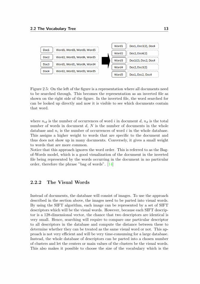
Text retrieval in documents follows some standard steps. The document isparted into words, and each word is represented by their stems. For example,”searching”, ”searched” and ”searches” would all become ”search”. Next, a stoplist is used to reject common words appearing in most documents such as ”the”and ”a”. Then, the document is represented by a vector indicating which wordsare appearing in the document and the number of times they appear.In the database of documents, all vectors representing the documents are or-ganized in an inverted file. An inverted file is structured so that each wordholds information about which document it appears in instead of each documentholding information about which words appears in it. This makes a search for aspecific word much faster, because only one lookup in the inverted file is neededto determine which documents contain that word. The structure is illustratedin Figure 2.5.Furthermore, a weight is assigned to each word, i, in a document d, such thatcommon words are weighted less than words that are specific for the given doc-ument. A common approach is given by:
wi =nidnd
logN
ni, (2.9)
2.2 The Vocabulary Tree 13
Figure 2.5: On the left of the figure is a representation where all documents needto be searched through. This becomes the representation as an inverted file asshown on the right side of the figure. In the inverted file, the word searched forcan be looked up directly and now it is visible to see which documents containthat word.
where nid is the number of occurrences of word i in document d, nd is the totalnumber of words in document d, N is the number of documents in the wholedatabase and ni is the number of occurrences of word i in the whole database.This assigns a higher weight to words that are specific to the document andthus does not show up in many documents. Conversely, it gives a small weightto words that are more common.Notice that this approach ignores the word order. This is referred to as the Bag-of-Words model, which is a good visualization of the document in the invertedfile being represented by the words occurring in the document in no particularorder, therefore the phrase ”bag of words”. [14]
2.2.2 The Visual Words
Instead of documents, the database will consist of images. To use the approachdescribed in the section above, the images need to be parted into visual words.By using the SIFT algorithm, each image can be represented by a set of SIFTdescriptors which will be the visual words. However, because each SIFT descrip-tor is a 128-dimensional vector, the chance that two descriptors are identical isvery small. Hence, searching will require to compare one particular descriptorto all descriptors in the database and compute the distance between these todetermine whether they can be treated as the same visual word or not. This ap-proach is not very efficient and will be very time-consuming for a large database.Instead, the whole database of descriptors can be parted into a chosen numberof clusters and let the centers or main values of the clusters be the visual words.This also makes it possible to choose the size of the vocabulary which is the
14 Theory and Implementation
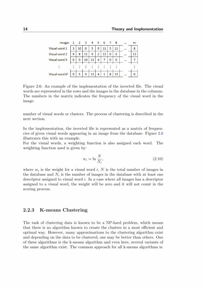
Figure 2.6: An example of the implementation of the inverted file. The visualwords are represented in the rows and the images in the database in the columns.The numbers in the matrix indicates the frequency of the visual word in theimage.
number of visual words or clusters. The process of clustering is described in thenext section.
In the implementation, the inverted file is represented as a matrix of frequen-cies of given visual words appearing in an image from the database. Figure 2.6illustrates this with an example.For the visual words, a weighting function is also assigned each word. Theweighting function used is given by:
wi = lnN
Ni, (2.10)
where wi is the weight for a visual word i, N is the total number of images inthe database and Ni is the number of images in the database with at least onedescriptor assigned to visual word i. In a case where all images has a descriptorassigned to a visual word, the weight will be zero and it will not count in thescoring process.
2.2.3 K-means Clustering
The task of clustering data is known to be a NP-hard problem, which meansthat there is no algorithm known to create the clusters in a most efficient andoptimal way. However, many approximations to the clustering algorithm existand depending on the data to be clustered, one may be better than others. Oneof these algorithms is the k-means algorithm and even here, several variants ofthe same algorithm exist. The common approach for all k-means algorithms is:

2.2 The Vocabulary Tree 15
1. Select k points as initial centers c2. Assign each data point x to its nearest center c3. Each center c is then updated to become the mean of all data
points assigned that center
The way the calculations are carried out varies from one approach to another.In this thesis, an algorithm written by Charles Elkan is used and it can be foundon Elkan’s website [5]. Elkan’s approach avoids unnecessary distance calcula-tions by applying triangle inequalities and thus, making the algorithm fasterand more effective on large datasets. The first triangle inequality used is givenby:
1: Let x be a data point and let c1 and c2 be two centers. If12d(c1, c2) ≥ d(x, c1) then d(x, c2) ≥ d(x, c1).
Here, d indicates the distance. For better understanding, an illustration ofthis setup is shown in Figure 2.7(a). Suppose x is a data point assigned tocenter c, and c′ is any other center. The distance d(x, c) is not known, only anupper bound u is known such that u ≥ d(x, c). According to the first triangleinequality, d(x, c) and d(x, c′) only needs to be computed if u > 1
2d(c, c′). Thissaves many computations because the distances between the centers only needto be computed once.The second triangle inequality used is given by:
2: Let x be a data point and let c1 and c2 be two centers. Thend(x, c2) ≥ max{0, d(x, c1)− d(x, c2)}.
This is a rewriting of the fact that the longest side of a triangle is always shorterthan the sum of the two other sides, which is illustrated in Figure 2.7(b). Sup-pose x is a data point assigned to center c, and c′ is the previous center thatx was assigned to. For the previous center c′ a lower bound l′ was known suchthat l′ ≤ d(x, c′), then a lower bound l for the new center c can be found as:
d(x, c) ≥ max{0, d(x, c′)− d(c, c′)} ≥ max{l′ − d(c, c′)} (2.11)
(a) (b)
Figure 2.7: The illustrations help to understand triangle inequality 1 and 2described above.

16 Theory and Implementation
l = max{l′ − d(c, c′)} (2.12)
Again, the already computed distance between the centers are used instead ofdistances from center to data point, which is what makes this algorithm fasterthan other k-means algorithms. [8][4]
2.2.4 The Tree Structure
By using the k-means algorithm, it is possible to create any number of visualwords. As described in section 2.2.2, each image is stored in the databaseas part of an inverted file. This means that for all images, the descriptors aredivided into the visual words they are most similar to and the approach involvescomparing every descriptor to every single visual word. If a large number ofvisual words are chosen, this becomes a very time-consuming process.A solution to this is hierarchical clustering which creates the tree structure.Instead of clustering the entire dataset into k groups, where k is the total numberof clusters, k will represent a sub-number or spreading factor. The approach isas follows; the entire dataset is parted into k clusters. Now for each of theseclusters, the process is repeated and each cluster is clustered into k new clustersor sub-clusters. This is repeated until some maximum level L is reached. Figure2.8 illustrates this in a 2-dimensional example for understanding purposes.
The efficiency of this structure becomes visible when a new descriptor is to beassigned to the cluster most similar to it. Instead of comparing the descriptor to
(a) (b)
Figure 2.8: (a) shows the 2-dimensional clustering of some sample data pointsinto 3 clusters, and afterwards, each of these are clustered into 3 new clusters.(b) shows the same clustering process as (a), but represented as a tree, whichmakes it easier to see the recursive approach with branching factor k = 3 andmaximum level L = 2.

2.3 Comparing Images 17
Figure 2.9: The two data points ended up in a cluster belonging to a centerwhich was not the nearest to the points.
all cluster centers, only k comparisons need to be computed for the first level, kfor the second level, and so on until the end of the tree is reached at level L. Inits entirety, that will be kL comparisons. As an example, say k = 4 and L = 5,then kL = 4 × 5 = 20 comparisons are needed. Without the tree structure, itwould have been kL = 45 = 1024 comparisons.An additional advantage when using the tree structure is the clustering efficiencyfor a large number of clusters. The k-means algorithm computes distances be-tween all centers, and the number of computations will grow exponentially withthe number of centers. In the tree structure, the number of centers in eachclustering process will always be small, even when the total number of clustersis large.The disadvantage of this approach is that it is not guaranteed that the descrip-tors are assigned to the nearest center. At each level, the cluster closest to aparticular descriptor is chosen. Thereafter, the search continues in the branchesof that cluster only and does not take the remaining clusters into account. Thiswill happen for every level which is the part that makes this searching strategymuch more efficient, but also open for errors. An example is shown in Figure 2.9where two points in the first clustering level are assigned the upper left center.In the next level of clustering, the new set of sub-centers in that cluster arecreated in a way that makes the two data points closer to one of the new centerscreated in a different cluster in the first level than the center they are currentlyassigned to. [13]
2.3 Comparing Images
When the structure of the database is created, the next step is to find a way tocompare query images with images in the database.By using an inverted file to store the images in the database, all images are
18 Theory and Implementation
indexed by the visual words they contain. The tree structure makes the indexingprocess much faster.The inverted file is structured such that the columns are unique histograms forthe images in the database. Hence, for a query image, such a histogram needsto be computed. This involves all descriptors to be assigned to one of the visualwords in the vocabulary by searching through the vocabulary tree. In eachlevel of the tree, the center with the shortest distance to the given descriptor ischosen. The distance is calculated as:
d(d, c) =√
(c− d) · (c− d), (2.13)
where d is the descriptor vector and c is the center vector. Since the distancesare for comparison only, there is no need to compute the square root. In total,this will be nkL dot-products, where n is the number of descriptors in the queryimage. The same computations were used for all images in the database whenthe database was created.To find a match in the database for a given query image, all images in thedatabase are given a score indicating how similar they are to the query image.The histogram of frequencies for each of the visual words for the query image qand an image in the database d are then assigned the weight from the weightingfunction:
qi = wini, (2.14)
di = wimi, (2.15)
where ni is the number of descriptors from the query image assigned visual wordi, and mi is the number of descriptors from the database image assigned visualword i, which is the same as the frequency in the inverted file. Now the scorefor these two vectors is computed as:
s(q,d) = ‖ q
‖q‖− d
‖d‖‖. (2.16)
The division by the norm makes the result invariant to the number of descriptorsassigned each of the images. The smaller the score, the more similar the imagesare.This score needs to be calculated for all images in the database and as thedatabase grows, so will the time for the scoring process. Here, the invertedfile shows its usefulness because only images known to contain certain visualwords will be of interest. By looking these visual words up in the inverted file,a list of images containing these words is returned. For the tests in this project,only small databases are used and therefore full use of the inverted file is notimplemented.

2.4 The Match Detector 19
2.4 The Match Detector
The previous sections described how to compare query images to the databaseimages and get a number of images returned in an order according to the sim-ilarity with the query image. However, this do not tell whether the imagesmatch the query image or not. They are just the system’s suggestion for possi-ble matches. An automatic process must be added to the system to determinewhether one of these images match the query image. In this section, the perfor-mance measure will be presented and based on that a threshold is chosen usinga ROC curve to pick out the correct matches. Furthermore, positions are addedto decrease the number of false matches.
2.4.1 Standard Deviation
By the look of the graph of scores between all images in the database and thequery image, the system performed well if, firstly, the correct image or imagesachieved the best score and secondly if the correct image or images are nicelyseparated from the rest of the images in score. Figure 2.10 shows an example ofthe graph for a matching image where the graph has a clear minimum or droparound the matching images from the database. The chosen match is the imagefrom the database with the lowest score. However, the graph looks like noisewhere no match should be found.An automatic selection of matches can be based on variance and deviations.The variance, σ2, indicates the variety in the graph:
σ2 =1
N
N∑i=1
(xi − µ)2, (2.17)
where x1, x2, ..., xn are the observations, N is the total number of observationsand µ is the mean value of the observations. The variance is not in the sameunits as the variables and is adjusted in the standard deviation: [7]
σ =√σ2 =
√√√√ 1
N
N∑i=1
(xi − µ)2. (2.18)
For the observation or image with the best score, the deviation from the meanis computed. If the deviation is greater than a chosen number of standarddeviations, the image is selected as a match. The threshold value to separatematches and non-matches is found with a ROC curve and is described furtherin the next section.

20 Theory and Implementation
Figure 2.10: This graph shows the score for all images in a database and a queryimage. The sudden drop in the score for some images in the database indicatesthat these images are significantly more similar to the query image than the restof the images in the database and can be assumed to be a match to the queryimage.
2.4.2 The ROC Curve
The Receiver Operating Characteristics (ROC) curve is a plot of the ratio be-tween true positives and false positives for a variation of threshold variables.It is used in classification problems where the instances are mapped to one oftwo classes, typically positives and negatives. Such a problem is visualized inthe confusion matrix in figure 2.11(a). The confusion matrix shows the fourgroups in the classification problem: true positives (TP ), false positives (FP ),true negatives (TN) and false negatives (FN). For a perfect classification, allinstances would be in the TP and TN groups which mean that no instancesare mapped to the wrong class. However, this is rarely the case, and the ROCcurve gives a visualization of the performance for a number of different thresh-old values used to part positives and negatives. From the confusion matrix, thetrue positive rate, TPR, and the false positive rate, FPR, are calculated as:
TPR =TP
P=
TP
TP + FN, (2.19)
FPR =FP
N=
FP
FP + TN, (2.20)
where P is the total number of positives and N is the total number of negatives.Figure 2.11(b) shows an example of the plot of the TPR versus the FPR whereeach point is representing a threshold value. The red line is the case whereTPR = FPR and thus the outcome if the instances were randomly mappedonto one of the two classes. For the perfect classification, as mentioned above,the point would be in the upper left corner. In general, the best performancesare reached for points close to the upper left corner or far away from the redline (but still in the top left part). [6]

2.4 The Match Detector 21
(a) Confusion matrix (b) Example plot of the ROC curve
Figure 2.11: The confusion matrix shows the grouping into true positives (TP ),false positives (FP ), true negatives (TN) and false negatives (FN) for a classi-fication problem. The ROC curve is an example taken from Figure 3.10 in thetest section. The points are nicely located along the top and right edges.
In the place recognition system that will be implemented, it is important that anadjustment or resetting of the position is not based on a false match. Thereforeit is desired for the FPR to be as small as possible or ideally zero for this system.This causes the TPR to decrease a large amount as well. Accordingly, not allpreviously visited places are recognized, but those that are recognized will allbe true.
2.4.3 Adding Positions
Using only standard deviations to determine whether the image that receivedthe best score is a match or not, will in some cases result in false matches. Thisis because an image that does not match received a better score than any of thetrue matches. In most cases, these errors can be eliminated by choosing a veryhigh threshold, but that will cause a decrease in the number of true matches aswell. A way to improve this is by adding positions.Instead of choosing the image from the database with the best score and thenaccepting it as a match if it is more than a certain number of standard deviationsfrom the mean value, a group of images are chosen beginning with the imagewith the best score, then the image with the second best score and so on. Theimages in this group then have to pass a position test. The position test isimplemented as follows; based on the five first query images, that is assumed

22 Theory and Implementation
to have a true match, the average distance between the present match and theprevious match is found. This is an average distance based on four distances.Then, for each new query image, the distance range of accepted images is givenby:
s = dµtk, (2.21)
where dµ is the average distance, t is the number of images since the last matchwas found and k is a factor indicating the number of allowed neighbors. So,for all possible matches in the group, if the distance between that particularpossible match and the previous match is larger than s, the match is discarded.After this position test, the image in the group with most standard deviationsfrom the mean value is chosen as a match. If none of the images in the grouppass the test, the best match will be chosen as the one with the best score, justlike before positions were added.This method is not ejecting matches, but instead looking for true matches in agroup of possible matches. If an image was to be ejected based on the positiontest alone, this would conflict with the idea of using a visual approach to detectpreviously visited places since an error in positions could cause that no matchespass the position test.

Chapter 3
Tests and Results
In this chapter, the system is tested to determine its performance in the loopclosing problem of detecting a previously visited place.To test the performance, the hit rate indicates how well the system performs.The hit rate is given as:
r =ncnp, (3.1)
where nc is the number of correct matches found by the system and np is thetotal number of matches.All the tests is carried out as if a robot had already gathered some informationand created a database from that. The query images sent into that databaseare separate tests and do not depend on one another. Only in the third test theinformation from the previous query images is used. The tests are focusing ondifferent parts of the system, here er short description of each of them
General Performance and Significance of the Vocabulary Size Herethe hit rate for dataset 1, 2 and 3 is computed for different vocabulary sizes todetermine the significance of the vocabulary size and the general performancefor the recognition system.

24 Tests and Results
Performance of the Match Detector The system used to automaticallydetermine whether a match is true or not is tested here, and the total perfor-mance is then the ratio of correct matches times the general hit rate found inthe previous tests.
Performance of the Match Detector with Positions Added These testsare carried out as a sequence of tests where each result is based on the previousresult in order to include the positions.
Unsuccessful Tests Results for these tests will not be shown in diagrams, asthe recognition system failed on the dataset used here. Instead some thoughtof the reason for this failure is described.
3.1 The Datasets
This section will give a description of the datasets used in the tests. In appendixB, some sample images from the datasets are shown.
3.1.1 Dataset 1
The images in this dataset are taken by an imaging robot of model houses. Theyhave the dimensions 1600x1200 pixel and an average of about 6,000 descriptors
Figure 3.1: Four images from first sequence and third sequence in dataset 1.Notice that the position of the camera inly differ in height.

3.1 The Datasets 25
assigned each image. The set consist of 3 sequences of 137 images where each ofthe sequences are taken in the same order from almost the same location. Onlythe height of the camera were different. An example for four of the images inthe first and the third sequence is shown in figure 3.1. In the tests, the firstsequence is used as the database and the third sequence is used as query images.
3.1.2 Dataset 2
The images in this dataset were taken in the city Silkeborg by a car drivingaround. Each image consists of 5 merged images covering a 360 degree viewwhich should make the system invariant to direction of the camera. The dimen-sions are 2000x1000 pixel and an average of 5,000 descriptors are assigned toeach image.40 images were chosen as the database such that they covered the same area as 65query images. Half of these query images has the same direction as the databaseimages and the other half has the opposite direction. In figure 3.2, three imagesfrom the database are shown together with the corresponding match from eachhalf of the set of query images.
Figure 3.2: The first row shows three sample images from the set used as thedatabase. The second and third row shows the query images corresponding tothe above images from the database. Images shown in row 2 are taken from thesame direction and images from row 3 are taken from the opposite direction.Notice the sun in the images in the third row and the switching of the right andleft side of the road.

26 Tests and Results
3.1.3 Dataset 3
Dataset 3 is almost similar to dataset 2. Each image is merged from 5 images,taken in the city Silkeborg. The dataset consists of 100 database images, 82query images that should be recognized and 41 query images that should notbe recognized. The query images have the same direction as the images in thedatabase.
Figure 3.3: The first row shows 3 sample images from database and the secondrow shows the matching query images. Notice the small variance in position.
3.1.4 Dataset 4
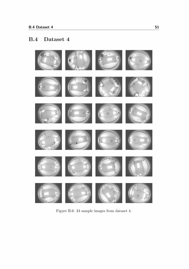
This dataset consists of images taken by a mobile robot on the corridors insidea building. The camera was pointing towards the ceiling on all images and thecamera used a fish eye lens to get a broader view. The images have the dimen-sions 640x480 pixel and an average of about 330 descriptors assigned to eachimage. Sample images from this dataset can be found in appendix B.
3.2 General Performance and Significance of theVocabulary Size
The first decision to take when using the visual text retrieval approach is thesize of the vocabulary. Here, the vocabulary size is that same as the number ofvisual words. As the vocabulary size increases, so does the time it takes to dothe calculations. However, a small vocabulary will not allow for much variation.

3.2 General Performance and Significance of the Vocabulary Size 27
Figure 3.4: The diagram shows the percentage of correct matches found for testsdone with different numbers of visual words.
In this section, a number of tests will be done with the vocabulary size rangingfrom 64 to over 10,000. The datasets 1, 2 and 3 are tested to see if the typeof dataset has any significance and to get an idea of the general ability torecognize an image. In the process of clustering, only 20-30% of the imagesfrom the dataset were used in order to make the clustering process faster. Thisdid not affect the results as long as the images chosen for the clustering processwere making a good representative for the entire dataset. By taking every 3rdto 5th image, all environmental changes would be included.The results of the tests are shown in figure 3.4 and the hit rate is computed asshown in equation 3.1.
Firstly the graph shows that the size of vocabulary where the hit rate reaches agood rate differs for the tree datasets. Dataset 1 needs only a small vocabularyof about 200 visual words to give a good performance. Whereas dataset 2 needsabout 2500 visual words before the hit rate rises. Dataset 3 needs about 10,000visual words to reach its peak, but around 6,000 to get results similar to theother datasets. The reason for this difference can be found in the variety in theimages from the datasets. Dataset 1 of the model houses does not vary muchfrom one another, where dataset 2 and 3 of the Silkeborg scenery varies moreand cannot be covered by a small number of visual words. Since both dataset2 and 3 are from the same environment, one might think that the number ofvisual words would be the same. The reason for this difference most likely hassomething to do with the size of the databases (40 images for dataset 2 and 100images for dataset 3). As mentioned before, the more variation, the larger thenumber of vocabulary is required which is confirmed here since there will bemore variation for 100 images than for 40.

28 Tests and Results
The peak values for the tree dataset at their respective optimal vocabulary sizebased on these tests are shown here:
Vocabulary size PeakDataset 1 253 83%Dataset 2 5,389 83%Dataset 3 10,276 83%
The curves for dataset 1 and 2 also show that once the peak of the hit rate isreached, increasing the vocabulary size does not affect the hit rate further. Thehit rate will stay relatively steady with a small oscillation margin. For bothdatasets, the hit rate ranges from 70% to 80% in the steady state. The reasonfor this big range is most likely that the tests are based on 137, 65 and 123query images respectively. More images would give a more precise value. Thecurve for dataset 3 reaches its peak at the end of the graph and it is not knownwhether it stays at the steady state. However, it seems reasonable to assumethat it does stay at the steady state since it followed the same curve up to thepeak just at a slower rate and shows a drop right after the peak.For each dataset, there is a minimum size of vocabulary tree for the system tobe able to run at all. If the vocabulary size is smaller than this value, eachvisual word in the vocabulary will have at least one descriptor from each imageassigned which causes the weight to be zero. With zero weight, the visual wordwill not be counted and there will be no vocabulary left when this happens toall of the visual words.The data for these tests are shown in appendix C together with the values of kand L in the tree structure and number of images used to create the vocabularytree. The values of k and L are given because the actual number of visual wordsrarely matches the theoretical number of visual words. In the clustering process
Figure 3.5: The graph shows that the system is able to find matches when thequery images (the x-axis) have the opposite camera direction than the databaseimages. The first half of the query images has the same direction and the secondhalf have the opposite direction.

3.3 Performance of the Match Detector 29
where the visual words are found, it often happens that a certain branch willrun out of descriptors assigned to that particular cluster before the end-nodesare reached. In this case, the center for the cluster at this level will be chosenand no further branching will be carried out resulting in fewer visual words.One last thing to notice about these tests is that the system was able to recognizeplaces in dataset 2 when the camera was pointing in the opposite direction.Although this was expected, Figure 3.5 confirms that. For all query images sentinto the database, the graph shows whether that particular image was assigneda correct match by the system. The first half of the query images had the samecamera direction as the database images and the second half had the oppositedirection. The graph also shows that it performs better when the images havethe same camera direction. This is due to the larger difference in position forthese images compared to the images with the camera pointing in the samedirection as the database images.
3.3 Performance of the Match Detector
In this test, dataset 3 was used. It has 100 images in the database, 82 queryimages that should be recognized and 41 query images that should not be rec-ognized. Figure 3.6 shows the score for all images in the database for both aquery image that is known to have a match in the database and for a queryimage that has no match in the database. On the x-axis is all of the databaseimages and on the y-axis the score for each of these images with the query im-
(a) The query image is recognized. (b) The query images is not recognized.
Figure 3.6: The graphs show database images on the x-axis and scores for eachof these images on the y-axis. In (a), the query image is known to have a matchin the database and the drop around database image 210 confirms that. Thequery image in (b) does not have a match in the database, which is confirmedby the noisy curve with no drop. The standard deviation for the query imagesis 4.59 and 2.56 respectively.

30 Tests and Results
ages. The smaller the score, the more similar the images are. For the queryimage known to have a match, a clear drop happens around database image 210which is known to be the true match for that query image. On the graph for theimage that should not find a match, no drop is present. The number of standarddeviations for the query images are 4.59 and 2.56 respectively. The automaticdetection of whether the best matching image for a given query image is true orfalse will be using standard deviations as described in section 2.4.1. To test theperformance of this method, the 123 query images from the dataset was sentinto the database. This was done for both a database with a vocabulary size of6,029 and 10,276 visual words which were found to give the highest hit rate inthe previous section. Figure 3.7 shows the correlation between the number ofstandard deviations from the mean and the match-status for each of the queryimages for the database using 6,029 visual words.
The next step is to determine the threshold value which is the number of stan-dard deviations that distinguishes true and false matches in the best possibleway. Figure 3.8 shows the ROC curve for both database sizes with threshold val-ues ranging from 1.5 to 5.1 standard deviations. No false matches are allowedin the system to detect previously visited places because they would cause awrong adjustment in the positions. The threshold is chosen to 3.4 standarddeviations for the 6,029 vocabulary size database which results in 12% of thepossible matches to be found and none of the query images without a match,would be given a false match.The final recognition rate can be calculated as the hit rate times the rate of true
Figure 3.7: The blue curve indicates the number of standard deviations from themean for each query image and the red line shows for each query image whethera true match was found, 1 if found and 0 otherwise. Notice the drop-tendencyin standard deviations when no match is found.

3.4 Performance of the Match Detector with Positions Added 31
(a) Database of 6,029 visual words (b) Database of 10,276 visual words
Figure 3.8: The ROC curve with threshold values ranging from 1.8 to 4 stan-dard deviations for (a) the 6,029 vocabulary size database and (b) the 10,276vocabulary size database.
matches found:rf = r × TPR = 79%× 12% = 8% (3.2)
Hence, 8% of the matches are found with no error.For the 10,276 vocabulary size database, the threshold value is chosen to 5.1standard deviations in order to eliminate false matches. A threshold value thislarge will cause a serious decrease in the total performance because the ratio oftrue matches is reduced to 2%:
rf = r × TPR = 83%× 2% = 1.7% (3.3)
In both cases the final recognition rate was decreased significantly in the processof selecting only true matches. A way to improve the system is by addingpositions to the database images.
3.4 Performance of the Match Detector with Po-sitions Added
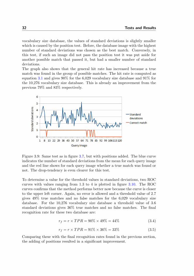
In an attempt to increase the total performance, positions are added to theimages and the process of finding a match is carried out as described in section2.4.3, with the factor k set to 6. The same tests were done as in previoussection. The results showed that the correlation between the number of standarddeviations from the mean value and the match status is even larger. Comparingthe graph in Figure 3.9 to the one in Figure 3.7, which are both from the 6,029
32 Tests and Results
vocabulary size database, the values of standard deviations is slightly smallerwhich is caused by the position test. Before, the database image with the highestnumber of standard deviations was chosen as the best match. Conversely, inthis test, if such an image did not pass the position test it was put aside foranother possible match that passed it, but had a smaller number of standarddeviations.The graph also shows that the general hit rate has increased because a truematch was found in the group of possible matches. The hit rate is computed asequation 3.1 and gives 90% for the 6,029 vocabulary size database and 91% forthe 10,276 vocabulary size database. This is already an improvement from theprevious 79% and 83% respectively.
Figure 3.9: Same test as in figure 3.7, but with positions added. The blue curveindicates the number of standard deviations from the mean for each query imageand the red line shows for each query image whether a true match was found ornot. The drop-tendency is even clearer for this test.
To determine a value for the threshold values in standard deviations, two ROCcurves with values ranging from 1.3 to 4 is plotted in figure 3.10. The ROCcurves confirms that the method performs better now because the curve is closerto the upper left corner. Again, no error is allowed and a threshold value of 2.7gives 49% true matches and no false matches for the 6,029 vocabulary sizedatabase. For the 10,276 vocabulary size database a threshold value of 3.6standard deviations gives 36% true matches and no false matches. The finalrecognition rate for these two database are:
rf = r × TPR = 90%× 49% = 44% (3.4)
rf = r × TPR = 91%× 36% = 33% (3.5)
Comparing these with the final recognition rates found in the previous section,the adding of positions resulted in a significant improvement.

3.5 Unsuccessful Tests 33
(a) Database of 6,029 visual words (b) Database of 10,276 visual words
Figure 3.10: The ROC curve with threshold values ranging from 1.8 to 4 stan-dard deviations for (a) the 6,029 vocabulary size database and (b) the 10,276vocabulary size database.
3.5 Unsuccessful Tests
The system has proven its worth for multiple datasets in the previous sections,but some restrictions apply to the dataset for the method to work properly.Tests were done with a dataset consisting of images taken by a mobile robot onthe corridors inside a building. The camera was pointing towards the ceiling onall images. Sample images from this dataset can be found in appendix B.A number of tests showed that the system did not perform well with theseimages. In fact, it was unable to find any matching images. Figure 3.11 showsthe 4 best matches found by the system for a query image, and none of thesewere correct. This happened for all the query images sent into the database.
Figure 3.11: Here are shown a query image and the 4 best matches found bythe recognition system. None of the found matches were correct.

34 Tests and Results
The reason for this can be found in the creation of the vocabulary tree where aquantization of the SIFT descriptors take place to create the visual words. Theimages from this dataset were assigned only about 330 descriptors each and aquantization of these would not leave much information about each image. Fur-thermore, since the images were all taken with a camera pointing towards theceiling, many images consisted of some similar areas, such as corners betweenwall and ceiling, doorframes and lamps.According to Boiman et al.[1], the quantization when creating the visual wordswill loose the most informative descriptors for each images. This is illustratedin Figure 3.12 where the figures represent the descriptors in the images. De-scriptors from 3 images are used to create 4 visual words. First the entire set ofdescriptors or figures are parted into 4 clusters and then an average in each clus-ter is found to represent the visual words which is represented by the assignedcolors. The images had a lot of similar descriptors and few specific descriptors,which resulted in the visual words being based on the most common descriptorswithout giving much influence to the specific descriptors.
Figure 3.12: 4 visual words are created from a database of 3 images. First allthe descriptors, represented by figures, are grouped into 4 groups and then arepresentative for each group is chosen as the visual word.

Chapter 4
Discussion
Based on the test results and the knowledge from the theory, this chapter dis-cusses the abilities and restrictions of the implemented system to detect alreadyvisited places. The performance of the system is separated into two parts.The first part is the ability to recognize an image also known as the generalrecognition system. The second part is the ability to distinguish between cor-rect recognized images and wrongly recognized images, otherwise known as thematch detector.
4.1 The General Recognition System
The results in the previous chapter have shown that it is possible to recognize aplace based on images only. Furthermore, the 83% hit rate shows that it worksvery well for the datasets used in the tests with the exception of dataset 4. TheSIFT algorithm has a big influence on the results, but using this algorithm alonewith no database or searching structure would make the system very inefficient.This was solved by introducing the vocabulary tree which led to a quantizationof the data size in the searching process by creating a number of visual wordsindexed in the tree structure. However, searching strategy improvement is alsothe reason the system did not work with dataset 4. For a dataset with littlevariance in the images and few interesting point for the SIFT algorithm, the

36 Discussion
quantization turned out to cause an elimination of the descriptors specific tothat particular image. Without the quantization, the SIFT algorithm wouldstill be able to distinguish the images, but would be very inefficient in the loopclosing problem where large databases will be needed.For the other datasets with plenty of descriptors and sufficient variance in im-ages, the quantization did what was hoped for; minimized the data size andmade a structure for searching possible. As mentioned in the section about thetree structure, it has the drawback that is it not guaranteed that each descriptoris assigned to the right visual word. However, in order to make a searching pro-cess more efficient, it is often necessary to accept some degree of error. Luckily,the error caused by this does not seem to influence the results badly.The tests also showed that the size of the vocabulary tree to receive the optimalresults depend on the dataset. Even when the images in the datasets are similar,the size is different. It also showed that after the peak has been reached, the hitrate does not decrease much for a larger number of visual words. This decreasecan just as well be noise from the small size of the database. In general, it isbetter to have a larger vocabulary than needed than to have a too small onebecause a vocabulary that is too small in size will cause a serious decrease inperformance, or even make the system useless.
4.2 The Match Detector
Up to now, the system has been finding the best match for a query image.Thanks to prior knowledge of whether that particular best match was correct ornot, the hit rate was established. Unfortunately, this is not enough if the systemneeds to be able to distinguish between previously visited places and unknownplaces. The system needs some rules to decide when a place or image can beaccepted as recognized. Here, the standard deviation was introduced becauseit indicates the general noise in the output graph. This can be used to detectrecognized places since they will typically be located outside of this standardzone as shown in Figure 2.10. As a result, a deviation from the mean value ofseveral standard deviations is obtained for a true matching image.The ROC curve was used to determine the best threshold value to distinguishbetween a true match and a false match in standard deviations. Since no falsematches are allowed, the rate of true matches could not get better than 12% inone case and 2% in another case. Combining these rates with the general hitrate, this leads to only 8% and 1.6% images to be recognized and accepted astrue recognitions.In order to increase the final recognition rate, positions were added to thedatabase images, which also increased the general hit rate such that the finalrecognition rate became 44% and 34% respectively. This is a large improvement

4.3 The Overall System 37
for both cases, but still not high enough to make the system a robust tool forloop detection. However, a small error could be allowed in order to increasethe hit rate if a position adjustment is based on a row of matches. This wouldminimize the possibility that a false match causes a redetermination of the loca-tion. Letting an adjustment being based on one recognition only is not robusteven if a threshold value is chosen not to allow any false matches. The systemis supposed to be able to work in an unknown environment and thus there isno guarantee that all false matches will have a number of standard deviationssmaller than those used to chose a threshold value.The adding of positions did not remove all false matches because its purposewas to moreover look for true matches rather than removing false matches. Aremoval of false matches based on the position alone would conflict with theidea of using an approach that is independent on the primary navigation tooland thus unaffected by a possible localization error. Making the match detectormore dependent on the positions would most likely result in a better perfor-mance until the error gets too large and too large of an error will cause therobot to not be able to detect if a loop is present.To increase the final recognition rate, a different method other than standarddeviation might work. Based on the tests, it seems like the threshold value instandard deviations varies for different databases, but four tests is not enoughto give a general judgement. However, even if a better method than using stan-dard deviation is found, the case where the general recognition system findsa wrong match with a clearly decipherable graph it would not do any better.Here, the best solution is to improve the general recognition system, so thatsuch confusion would never happen.
4.3 The Overall System
The best matches found by the system do not always happen to be at the exactsame location. Most of the time, it would be close enough so that all surround-ings are the same. This means that the system does not work if exact positioningis wanted. This is caused by the SIFT algorithm’s ability to recognize objectsfrom different angles which is practical if the robot should be able to recognizea place if it is not in the exact same spot.To optimize the localization, multiple cameras can be used instead of just one,as was done in dataset 2 and 3. The quadrangles in Figure 4.1 represent a robotin two different locations. With only one camera, the image from both locationswould show the circle and a little varying background. If two cameras are used,the images from the front camera would still be almost similar, but the cameraspointing backwards would create two different images.

38 Discussion
Figure 4.1: The quadrangles are representing a robot at two different locations.With only one camera in the front, the positions would seem the same for bothlocations. By adding a camera in the back, the robot will be able to differbetween these two locations.
This would also minimize the number of wrongly recognized images with clearlyreadable graphs. For dataset 1, the distribution of correct matches is foundin Figure 4.2. It shows that for a group of query images, no correct matcheswere found. For all these query images, the graphs with scores for each of thedatabase images all had a drop as the sample in Figure 2.10. However, the dropturned out to be at a wrong image. Having two cameras could have preventedthis because the possibility that the two cameras will find corresponding wrongmatches is very little.
Figure 4.2: This graph shows the 137 query images on the x-axis and whethera correct match was found in the y-axis. Around query image 40-57, no correctmatches were found.
4.4 Future Work
To begin with, an improvement of the general recognition system would be veryinteresting. For example, adding colors to the SIFT descriptors might increasethe hit rate and maybe make the correct matches stand out more clearly. Thiswill make it easier for the match detector to distinguish between true and falsematches and it might be possible to chose a general threshold value. It would

4.4 Future Work 39
be interesting to see how much this could be improved.If adding colors can increase the performance, it would also be very interestingto implement it in a robot and see how it works in real life. However, thisis a rather large project as the current system is implemented in Matlab, andrequires manually calls to the functions.Furthermore, an implementation of the scoring where the advantages of theinverted file is used would be of interest since it allows an application of largerdatabases.

40 Discussion

Chapter 5
Conclusion
The implementation of the system to detect a previously visited place has shownthat this is possible by using images to represent the places. Using the SIFTalgorithm to extract information about the images, the Bag-of-Words modelto store the information in a database and the vocabulary tree to create andsearch in the database did all work well, and had a maximum recognition rateof 91%. However, if this is going to work in a real robot, the system needs tobe improved because the separation of correct recognized places and wronglyrecognized places needs a clear boundary between the two categories in orderto be able to detect a majority of the correct recognized places without error.As the system is now, the maximum detection rate of previously visited places is44% with no error. Although better performance is preferred for implementationin a robot, it shows that the method used in the system works.

42 Conclusion

Appendix A
Mathematical Review
A.1 The Hessian Matrix
The Hessian matrix is the matrix of second order partial derivatives of a multi-variable function. Say we have a function, f , with two variables, x and y, thenthe Hessian matrix would look like this:
H =
[fxx fxyfyx fyy
]. (A.1)
Here fxx is the derivative of f with respect to x, and then the derivative of thiswith respect to x again, fxy is the derivative of f with respect to x, and thenthe derivative of this with respect to y and so on, as shown here:
fxx =∂2f
∂x2,
fxy =∂2f
∂x∂y, (A.2)
fyy =∂2f
∂y2,
fyx =∂2f
∂y∂x.

44 Mathematical Review
Appendix B
Datasets
This appedix will show some sample images from the datasets used in the tests.The images are chosen to both indicate the difference between adjacent imagesand give an idea of how the variation in the dataset.For each dataset the query images are not part of the database, but are takenin the same way as the images in the database. This means that only a smallvariation in position distinguishes these from the images shown here.

46 Datasets
B.1 Dataset 1
Figure B.1: The first 24 of the images used to create the database.
B.1 Dataset 1 47
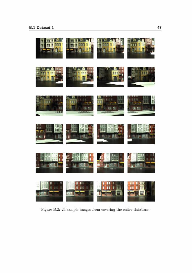
Figure B.2: 24 sample images from covering the entire database.

48 Datasets
B.2 Dataset 2
Figure B.3: The first 21 of the images used to create the database.

B.3 Dataset 3 49
B.3 Dataset 3
Figure B.4: The first 18 of the images used to create the database.

50 Datasets
Figure B.5: 18 sample images from dataset 3 covering the entire database.
B.4 Dataset 4 51
B.4 Dataset 4
Figure B.6: 24 sample images from dataset 4.

52 Datasets

Appendix C
Testresults
Dataset 1k L skip Theoretically vo-
cabulary sizeActual vocabularysize
Hit rate
4 3 5 64 64 66%4 4 5 256 253 83%7 3 5 343 343 82%5 4 5 625 617 74%6 4 5 1296 1251 78%5 5 5 3125 2725 71%8 4 5 4096 3501 75%6 7 5 7776 5926 74%5 6 5 15625 7157 78%
54 Testresults
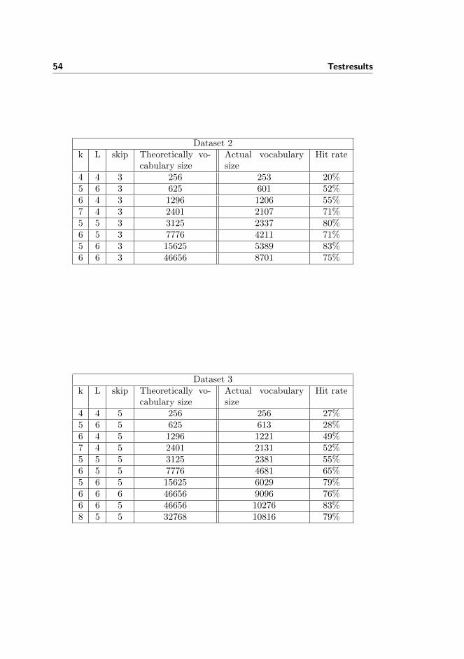
Dataset 2k L skip Theoretically vo-
cabulary sizeActual vocabularysize
Hit rate
4 4 3 256 253 20%5 6 3 625 601 52%6 4 3 1296 1206 55%7 4 3 2401 2107 71%5 5 3 3125 2337 80%6 5 3 7776 4211 71%5 6 3 15625 5389 83%6 6 3 46656 8701 75%
Dataset 3k L skip Theoretically vo-
cabulary sizeActual vocabularysize
Hit rate
4 4 5 256 256 27%5 6 5 625 613 28%6 4 5 1296 1221 49%7 4 5 2401 2131 52%5 5 5 3125 2381 55%6 5 5 7776 4681 65%5 6 5 15625 6029 79%6 6 6 46656 9096 76%6 6 5 46656 10276 83%8 5 5 32768 10816 79%
Appendix D
Running the Software
To allow the reader to test the system, the Matlab source code and images fromdataset 3 is attached on a CD. All content needs to be transferred to the com-puter.In order to test the system, the ”Software” folder needs to be opened in Matlab.To create the database, enter createDatabase. Inside the createDatabase.mfile, the values for k, L, skip and number of images wanted in the database canbe chosen. The creation of the database takes a while. The available image dataallows a database of maximum 100 images.When the database is created, enter start to start the system. This commandresets the positionlog. For each query image, enter inputImage(imageNo) whereimageNo is the query image number. The available image data allows numbers78-200. The system will tell whether it has found a match or not plus plottinga graph showing the difference between the query image and all images in thedatabase. This graph is similar to the one in Figure 2.10To get the system to work optimally, the first query images need to be image78, 79, 80, 81 and 82 in that order.

56 Running the Software

Bibliography
[1] Oren Boiman, Eli Shechtman, and Michal Irani. In defense of nearest-neighbor based image classification. Computer Vision and Pattern Recog-nition, pages 1–8, June 2008.
[2] Jonas Callmer, Karl Granstrom, J. Nieto, and F. Ramos. Tree of wordsfor visual loop closure detection in urban slam. In Jonghyuk Kim andRobert Mahony, editors, Proceedings of the 2008 Australasian Conferenceon Robotics and Automation, page 8, December 2008.
[3] Hugh Durrant-Whyte and Tim Bailey. Simultaneous localisation and map-ping (slam): Part i the essential algorithms. IEEE Robotics and AutomationMagazine, 2:99–110, 2006.
[4] Charles Elkan. Using the triangle inequality to accelerate k-means. In Pro-ceedings of the Twentieth International Conference on Machine Learning,2003.
[5] Charles Elkan. Software: K-means algorithm. Downloaded fromhttp://cseweb.ucsd.edu/ elkan/fastkmeans.html, 2004.
[6] Tom Fawcett. An introduction to ROC analysis. Pattern Recognition Let-ters, 27(8):861–874, June 2006.
[7] Richard A. Johnson. Probability and Statistics for Engineers, chapter 4.4.Pearson Prentice Hall, 7th edition, 2005.
[8] Tapas Kanungo, David M. Mount, Nathan S. Netanyahu, Christine D.Piatko, Ruth Silverman, and Angela Y. Wu. An efficient k-means clusteringalgorithm: Analysis and implementation. IEEE Transactions on PatternAnalysis and Machine Intelligence, 24(7):881–892, July 2002.

58 BIBLIOGRAPHY
[9] David G. Lowe. Distinctive image features from scale-invariant keypoints.International Journal of Computer Vision, 60(2):91–110, 2004.
[10] David G. Lowe. Software: Sift-keypoint detector. Downloaded fromhttp://www.cs.ubc.ca/ lowe/keypoints/, 2005.
[11] Paul Newman and Kin Leong Ho. Slam- loop closing with visually salientfeatures. IEEE Robotics and Automation Magazine, pages 635–642, 2005.
[12] Paul Newman and Kin Leong Ho. Detecting loop closure with scene se-quences. International Journal of Computer Vision, 74(3):261–286, septem-ber 2007.
[13] David Nister and Henrik Stewenius. Scalable recognition with a vocabularytree. In Proceedings of IEEE Conference on Computer Vision and PatternRecognition (CVPR), volume 2, pages 2131–2168, 2006.
[14] Josef Sivic and Andrew Zisserman. Video Google: A text retrieval approachto object matching in videos. In Proceedings of the International Conferenceon Computer Vision, volume 2, pages 1470–1477, October 2003.