Group RESEARCH ACTIVITY

OF

LORENZ EQUATION

Sir. MAQSOOD ALAM

( HUMANITIES )

Muhammad Abdullah soleh ( ME # 131023 )

Introduction

For many people working in the physical sciences, the butterfly effect is a well-

known phrase. But even if you are unacquainted with the term, its consequences are

something you are intimately familiar with.

Edward Lorenz investigated the feasibility of performing accurate, long-term

weather forecasts, and came to the conclusion that even something as seemingly

insignificant as the flap of a butterfly’s wings can have an influence on the weather on the

other side of the globe. This implies that global climate modelers must take into account

even the tiniest of variations in weather conditions in order to have even a hope of being

accurate. Some of the models used today in weather forecasting have up to a million

unknown variables!

With the advent of modern computers, many people believed that accurate

predictions of systems as complicated as the global weather were possible. Lorenz’ studies,

both analytical and numerical, were concerned with simplified models for the flow of air in

the atmosphere. He found that even for systems with considerably fewer variables than the

weather, the long-term behavior of solutions is intrinsically unpredictable. He found that

this type of non-periodic, or chaotic behavior, appears in systems that are described by non-

linear differential equations.

The atmosphere is just one of many hydro dynamical systems, which exhibit a

variety of solution behavior: some flows are steady; others oscillate between two or more

states; and still others vary in an irregular or haphazard manner. This last class of behavior in

a fluid is known as turbulence or in more general systems as chaos. Examples of chaotic

behavior in physical systems include:-

• Thermal convection in a tank of fluid, driven by a heated plate on the bottom, which

displays an irregular patter of “convection rolls” for certain ranges of the temperature

gradient;

• A rotating cylinder, filled with fluid, that exhibits regularly-spaced waves or irregular, non-

periodic flow patterns under different conditions;

• The Lorenz Ian water wheel, a mechanical system.

Q1) CRITICAL POINT CALCULATION:

( ) ( )

( )

( )

Here:

From Equation ( 1 ) we get :

( )

From Equation ( 2 ) :

As : x = y

( )

From Equation ( 3 ) :

As: b =

, x=y and z = r – 1, above equation becomes

( )

( )

√

( )

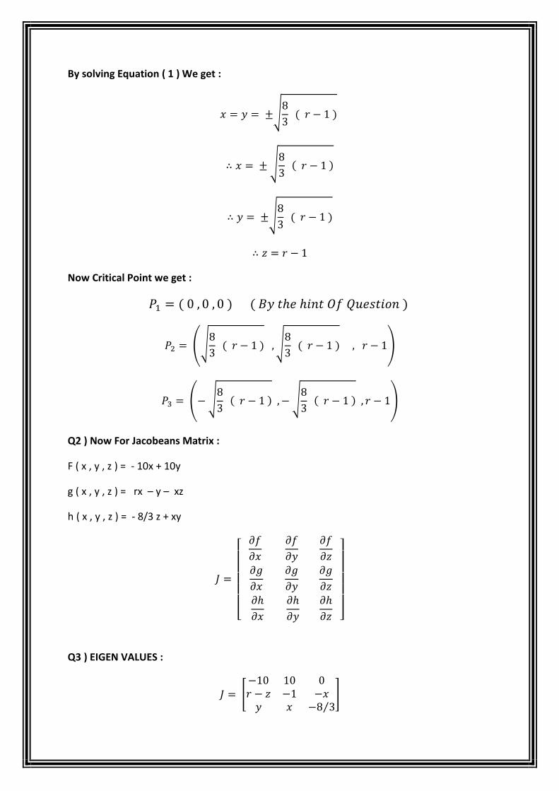
By solving Equation ( 1 ) We get :

√

( )

√

( )

√

( )

Now Critical Point we get :

( ) ( )

(√

( ) √

( ) )

( √

( ) √

( ) )

Q2 ) Now For Jacobeans Matrix :

F ( x , y , z ) = - 10x + 10y

g ( x , y , z ) = rx – y – xz

h ( x , y , z ) = - 8/3 z + xy

[

]

Q3 ) EIGEN VALUES :

[ ⁄

]

( ) [ ⁄

]

( ( ) )

[ ⁄

] [

]

[

( ) ⁄

]

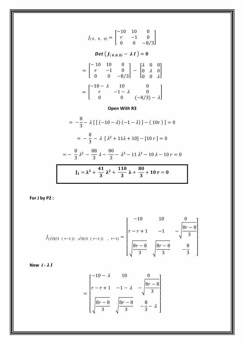
Open With R3

[ [ ( ) ( ) ] ( ) ]

[ ] [ ]

For J by P2 :

( ( ( )) ( ( )) )

[

√

√

√

]

Now J -

[

√

√

√

]

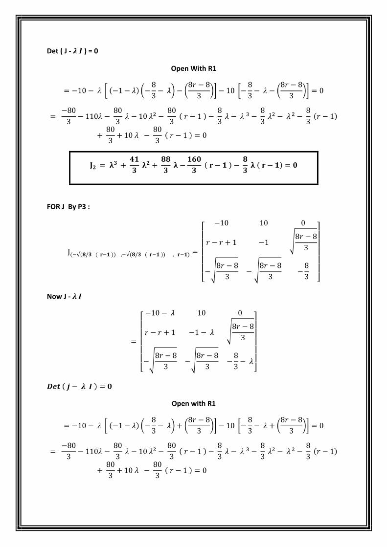
Det ( J - ) = 0

Open With R1

[ ( ) (

) (

)] [

(

)]

( )

( )

( )

( )

( )

FOR J By P3 :

( ( ( )) ( ( )) )

[

√

√

√

]

Now J -

[

√

√

√

]

( )

Open with R1

[ ( ) (

) (

)] [

(

)]

( )

( )

( )

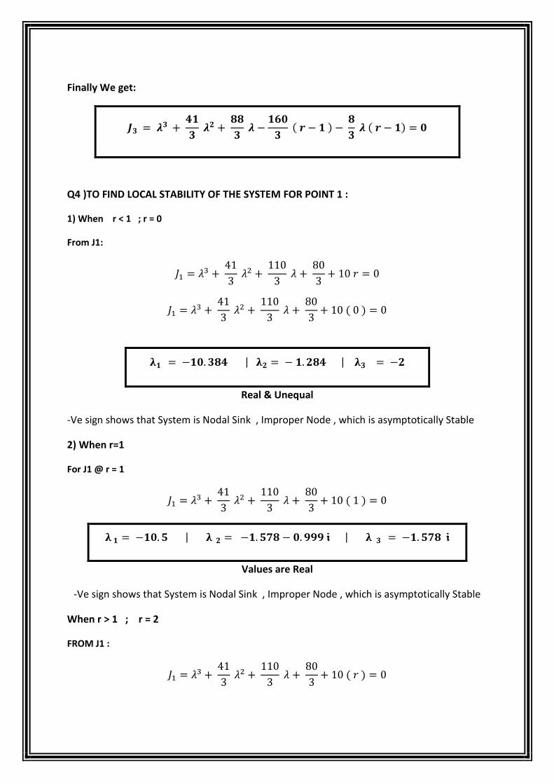
Finally We get:

( )

( )

Q4 )TO FIND LOCAL STABILITY OF THE SYSTEM FOR POINT 1 :

1) When r < 1 ; r = 0

From J1:

( )

| |

Real & Unequal

-Ve sign shows that System is Nodal Sink , Improper Node , which is asymptotically Stable

2) When r=1

For J1 @ r = 1

( )

| |

Values are Real

-Ve sign shows that System is Nodal Sink , Improper Node , which is asymptotically Stable

When r > 1 ; r = 2

FROM J1 :

( )

( )

| |

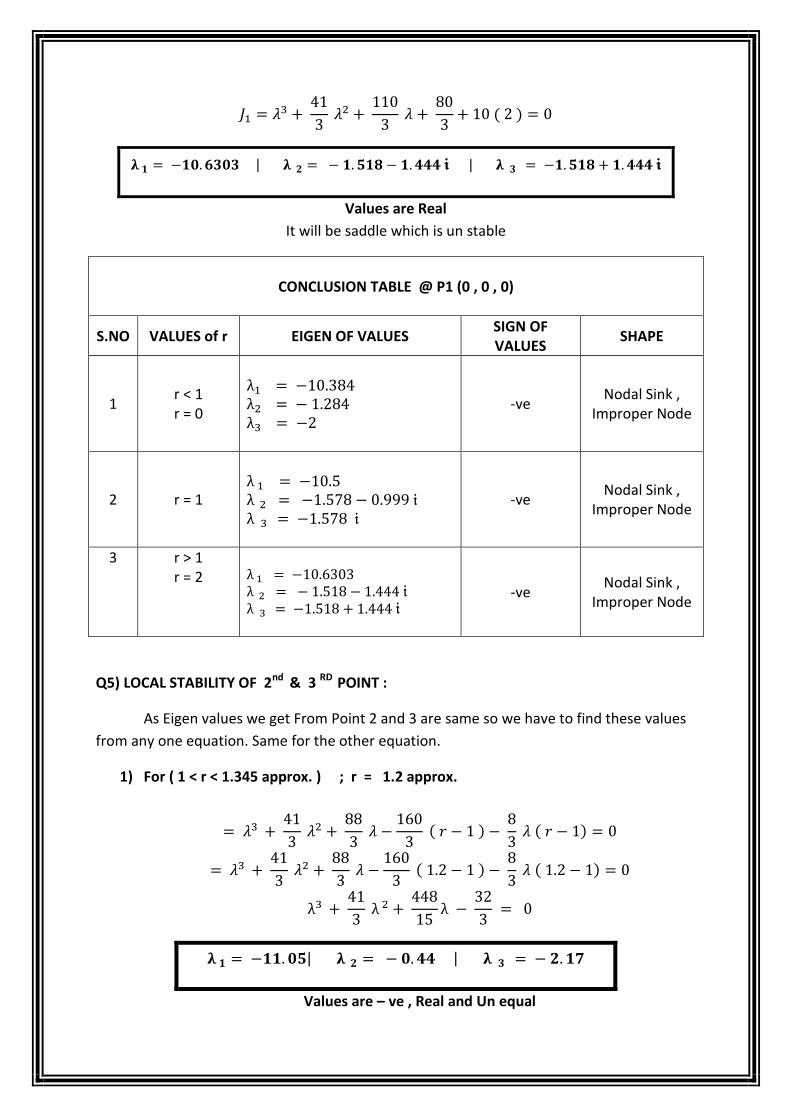
Values are Real

It will be saddle which is un stable

CONCLUSION TABLE @ P1 (0 , 0 , 0)

S.NO VALUES of r EIGEN OF VALUES SIGN OF VALUES

SHAPE

1 r < 1 r = 0

-ve Nodal Sink ,

Improper Node

2 r = 1

-ve Nodal Sink ,

Improper Node

3 r > 1 r = 2

-ve Nodal Sink ,

Improper Node

Q5) LOCAL STABILITY OF 2nd & 3 RD POINT :

As Eigen values we get From Point 2 and 3 are same so we have to find these values

from any one equation. Same for the other equation.

1) For ( 1 < r < 1.345 approx. ) ; r = 1.2 approx.

( )

( )

( )

( )

| |

Values are – ve , Real and Un equal

The system will Nodal Sink , Improper Node which is asymptotically stable called

stable & Attractive

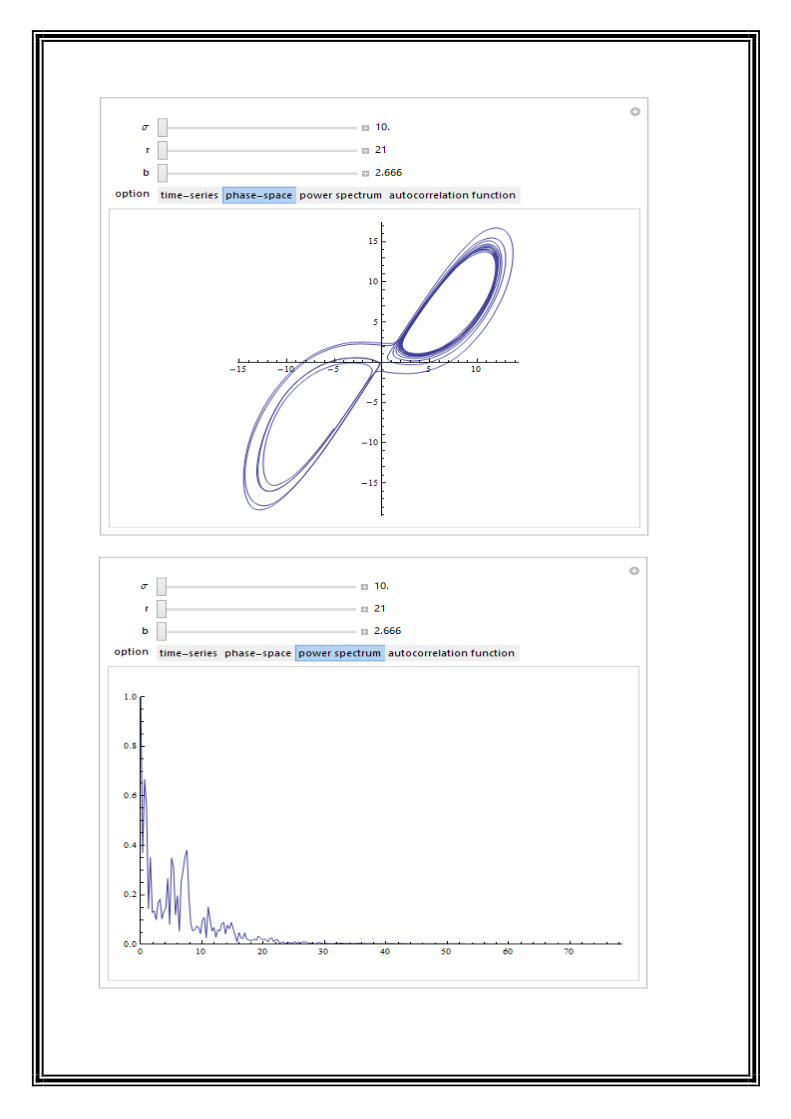
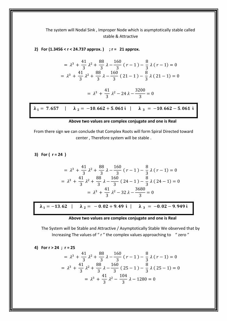
2) For (1.3456 < r < 24.737 approx. ) ; r = 21 approx.

( )

( )

( )

( )

| |

Above two values are complex conjugate and one is Real

From there sign we can conclude that Complex Roots will form Spiral Directed toward

center , Therefore system will be stable .

3) For ( r = 24 )

( )

( )

( )

( )

| |

Above two values are complex conjugate and one is Real

The System will be Stable and Attractive / Asymptotically Stable We observed that by

Increasing The values of “ r ” the complex values approaching to “ zero ”

4) For r > 24 ; r = 25

( )

( )

( )

( )

| |

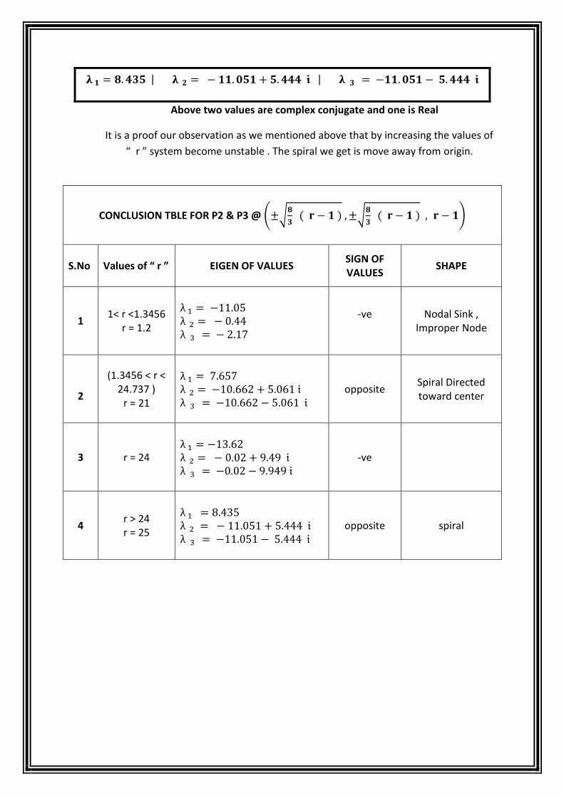
Above two values are complex conjugate and one is Real

It is a proof our observation as we mentioned above that by increasing the values of

“ r ” system become unstable . The spiral we get is move away from origin.

CONCLUSION TBLE FOR P2 & P3 @ ( √

( ) √

( ) )

S.No

Values of “ r ” EIGEN OF VALUES

SIGN OF VALUES

SHAPE

1

1< r <1.3456 r = 1.2

-ve

Nodal Sink , Improper Node

2

(1.3456 < r < 24.737 )

r = 21

opposite Spiral Directed toward center

3

r = 24

-ve

4

r > 24 r = 25

opposite spiral

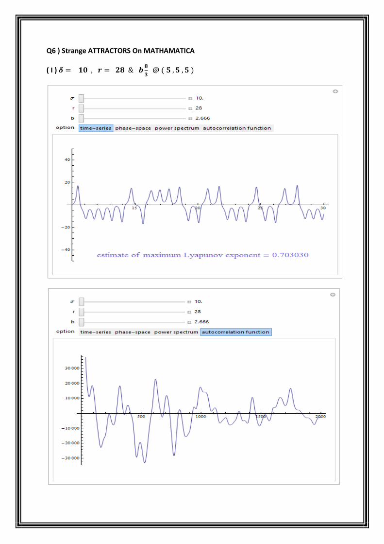
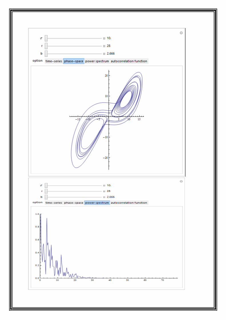
Q6 ) Strange ATTRACTORS On MATHAMATICA

( I )

( )

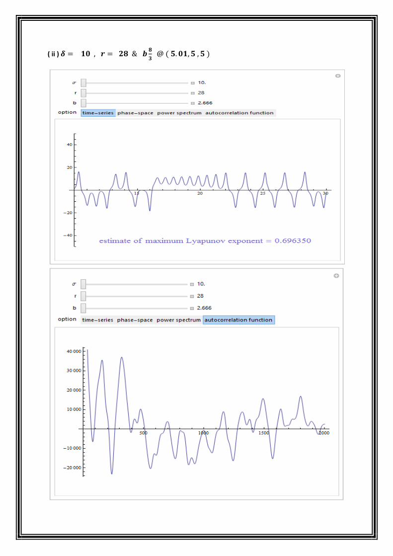
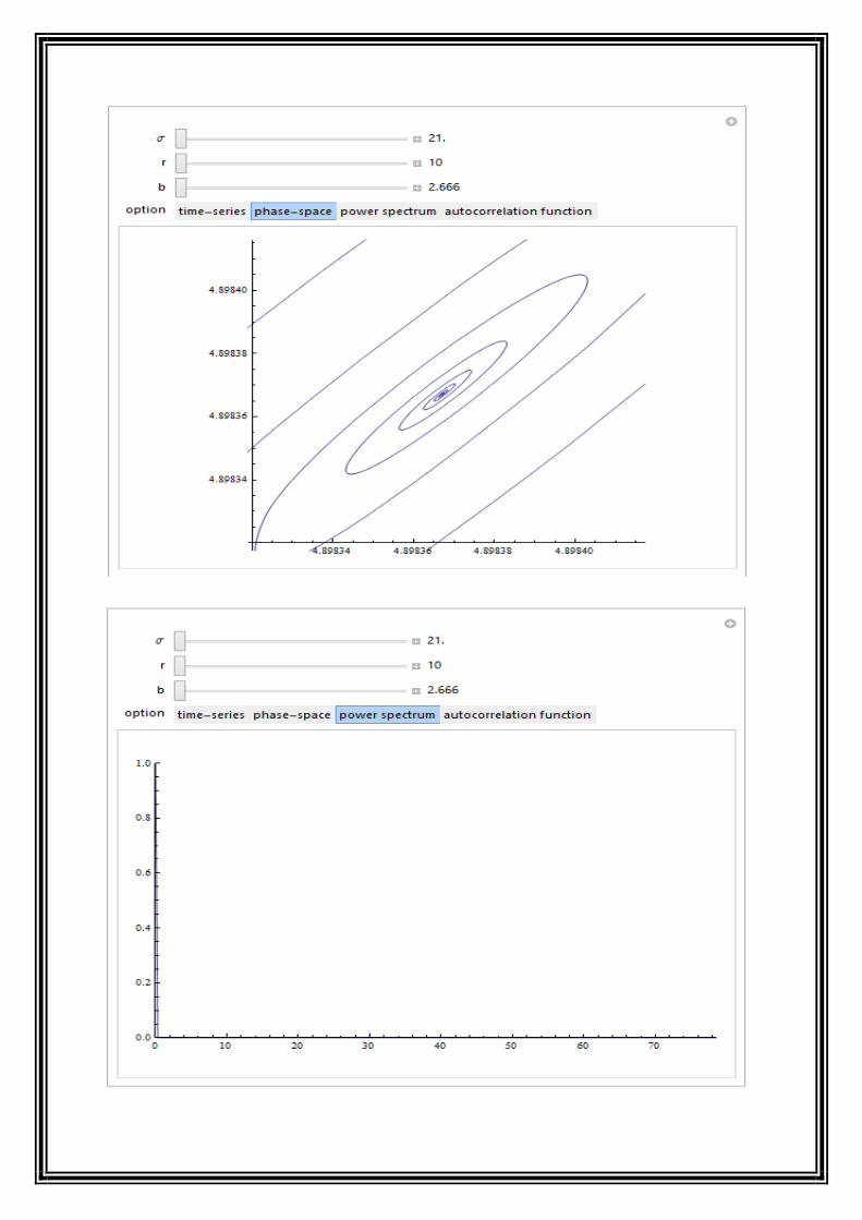
( ii )

( )

(iii)

( )

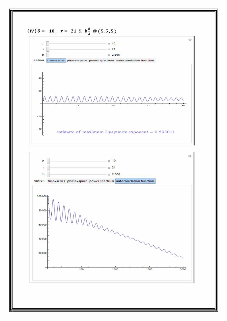
( IV )

( )

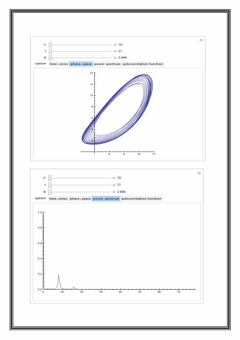
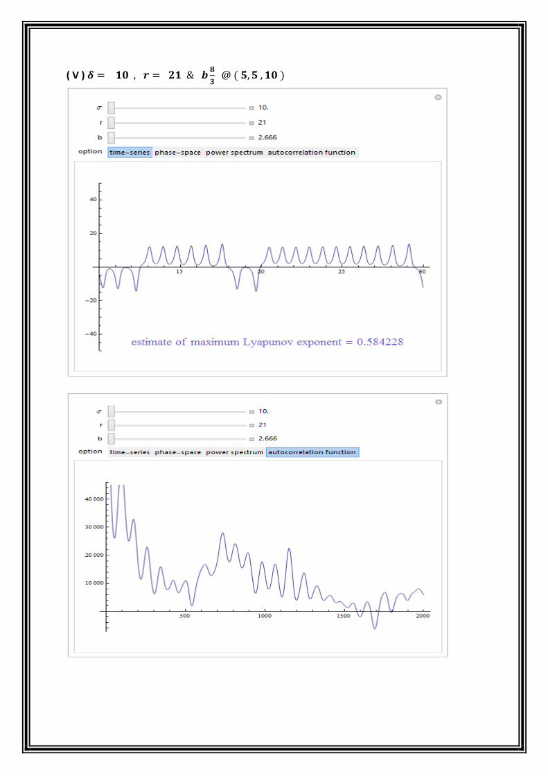
( V )

( )