lorenzo rosasco - massachusetts institute of technology
TRANSCRIPT

Introductory Machine Learning Notes1
Lorenzo RosascoDIBRIS, Universita’ degli Studi di Genova
LCSL, Massachusetts Institute of Technology and Istituto Italiano di [email protected]
December 21, 2017
1
These notes are an attempt to extract essential machine learning concepts for beginners. They are a draft and will be updated.Likely they won’t be typos free for a while. They are dry and lack examples to complement and illustrate the general ideas.Notably, they also lack references, that will (hopefully) be added soon. The mathematical appendix is due to Andre Wibisono’snotes for the math camp of the 9.520 course at MIT.

ABSTRACT. Machine Learning has become a key to develop intelligent systems and analyze data in scienceand engineering. Machine learning engines enable systems such as Siri, Kinect or the Google self driving car,to name a few examples. At the same time machine learning methods help deciphering the information in ourDNA and make sense of the flood of information gathered on the web. These notes provide an introductionto the fundamental concepts and methods at the core of modern machine learning.

Contents
Chapter 1. Statistical Learning Theory 11.1. Data 11.2. Probabilistic Data Model 11.3. Loss Function and and Expected Risk 21.4. Stability, Overfitting and Regularization 2
Chapter 2. Local Methods 52.1. Nearest Neighbor 52.2. K-Nearest Neighbor 62.3. Parzen Windows 62.4. High Dimensions 7
Chapter 3. Bias Variance and Cross-Validation 93.1. Tuning and Bias Variance Decomposition 93.2. The Bias Variance Trade-Off 103.3. Cross Validation 10
Chapter 4. Regularized Least Squares 114.1. Regularized Least Squares 114.2. Computations 114.3. Interlude: Linear Systems 124.4. Dealing with an Offset 12
Chapter 5. Regularized Least Squares Classification 135.1. Nearest Centroid Classifier 135.2. RLS for Binary Classification 145.3. RLS for Multiclass Classification 14
Chapter 6. Feature, Kernels and Representer Theorem 156.1. Feature Maps 156.2. Representer Theorem 156.3. Kernels 16
Chapter 7. Regularization Networks 197.1. Empirical Risk Minimization 197.2. Hypotheses Space 197.3. Tikhonov Regularization and Representer Theorem 207.4. Loss Functions and Target Functions 20
Chapter 8. Logistic Regression 238.1. Interlude: Gradient Descent and Stochastic Gradient 238.2. Regularized Logistic Regression 248.3. Kernel Regularized Logistic Regression 258.4. Logistic Regression and Confidence Estimation 25
Chapter 9. From Perceptron to SVM 279.1. Perceptron 279.2. Margin 279.3. Maximizing the Margin 289.4. From Max Margin to Tikhonov Regularization 29
iii

iv CONTENTS
9.5. Computations 299.6. Dealing with an off-set 29
Chapter 10. Dimensionality Reduction 3110.1. PCA & Reconstruction 3110.2. PCA and Maximum Variance 3210.3. PCA and Associated Eigenproblem 3210.4. Beyond the First Principal Component 3210.5. Singular Value Decomposition 3310.6. Kernel PCA 33
Chapter 11. Variable Selection 3511.1. Subset Selection 3511.2. Greedy Methods: (Orthogonal) Matching Pursuit 3511.3. Convex Relaxation: LASSO & Elastic Net 36
Chapter 12. Density Estimation & Related Problems 3912.1. Density estimation 3912.2. Applications of Density Estimation to Other Problems 40
Chapter 13. Clustering Algorithms 4313.1. K-Means 4313.2. Hierarchical Clustering 4413.3. Spectral Clustering 44
Chapter 14. Graph Regularization 4714.1. Graph Labelling via Regularization 4714.2. Transductive and Semi-Supervised Learning 48
Chapter 15. Bayesian Learning 4915.1. Maximum Likelihood Estimation 4915.2. Maximum Likelihood for Density Estimation 4915.3. Maximum Likelihood for Linear Regression 5015.4. Prior and Posterior 5015.5. Beyond Linear Regression 51
Chapter 16. Neural Networks 5316.1. Deep Neural Networks 5416.2. Estimation and Computations in DNN 5516.3. Convolutional Neural Networks 56
Chapter 17. A Glimpse Beyond The Fence 5717.1. Different Kinds of Data 5717.2. Data and Sampling Models 5717.3. Learning Approaches 5717.4. Some Current and Future Challenges in Machine Learning 58
Appendix A. Mathematical Tools 59A.1. Structures on Vector Spaces 59A.2. Matrices 60

CHAPTER 1
Statistical Learning Theory
Machine Learning deals with systems that are trained from data rather than being explicitly pro-grammed. Here we describe the data model considered in statistical learning theory.
1.1. Data
The goal of supervised learning is to find an underlying input-output relation
f(xnew) ∼ y,given data.The data, called training set, is a set of n input-output pairs,
S = (x1, y1), . . . , (xn, yn).Each pair is called an example or sample, or data point. We consider the approach to machine learningbased on the so called learning from examples paradigm.
Given the training set, the goal is to learn a corresponding input-output relation. To make sense ofthis task, we have to postulate the existence of a model for the data. The model should take into accountthe possible uncertainty in the task and in the data.
1.2. Probabilistic Data Model
The inputs belong to an input space X , we assume throughout that X ⊆ RD. The outputs belongto an output space Y . We consider several possible situations: regression Y ⊆ R, binary classificationY = −1, 1 and multi-category (multiclass) classification Y = 1, 2, . . . , T. The space X × Y is calledthe data space.
We assume there exists a fixed unknown data distribution p(x, y) according to which the dataare identically and independently distributed (i.i.d.) 1. The probability distribution p models differentsources of uncertainty. We assume that it factorizes as p(x, y) = pX(x)p(y|x), where
• the conditional distribution p(y|x), see Figure 1, describes a non deterministic relation betweeninput and output.
• The marginal distribution pX(x) models uncertainty in the sampling of the input points.
YX
p (y|x)
x
FIGURE 1. For each input x there is a distribution of possible outputs p(y|x) (yellow).The green area is the distribution of all possible outputs.
1

2 1. STATISTICAL LEARNING THEORY
We provide two classical examples of data model, namely regression and classification.
EXAMPLE 1 (Regression). In regression the following model is often considered y = f∗(x) + ε. Here f∗ isa fixed unknown function, for example a linear function f∗(x) = xTw∗ for some w∗ ∈ RD and ε is random noise,e.g. standard Gaussian N (0, σ), σ ∈ [0,∞). See Figure 2 for an example.
EXAMPLE 2 (Classification). In binary classification a basic example of data model is a mixture of twoGaussians, i.e. p(x|y = −1) = 1
ZN (−1, σ−), σ− ∈ [0,∞) and p(x|y = 1) = 1ZN (+1, σ+), σ+ ∈ [0,∞), where
1Z is a suitable normalization. For example in classification, a noiseless situation corresponds to p(1|x) = 1 or 0for all x.
1.3. Loss Function and and Expected Risk
The goal of learning is to estimate the “best” input-output relation, rather than the whole distribu-tion p.
More precisely, we need to fix a loss function
` : Y × Y → [0,∞),
which is a (point-wise) measure of the error `(y, f(x)) we incur in when predicting f(x) in place of y.Given a loss function, the ”best” input-output relation is the target function f∗ : X → Y minimizing theexpected loss (or expected risk)
E(f) = E[`(y, f(x))] =
∫dxdyp(x, y)`(y, f(x)).
which can be seen as a measure of the error on past as well as future data. The target function cannot becomputed since the probability distribution p is unknown. A (good) learning algorithm should providea solution that behaves similarly to the target function, and predict/classify well new data. In this case,we say that the algorithm generalizes.
REMARK 1 (Decision Surface/Boundary). In classification we often visualize the so called decision bound-ary (or surface) of a classification solution f . The decision boundary is the level set of points x for which f(x) = 0.
1.4. Stability, Overfitting and Regularization
A learning algorithm is a procedure that given a training set S computes an estimator fS . Ideally,an estimator should mimic the target function, in the sense that E(fS) ≈ E(f∗). The latter requirementneeds some care since fS depends on the training set and hence is random. For example, one possibilityis to require an algorithm to be good in expectation, in the sense that
ES [E(fS)− E(f∗)],
is small.More intuitively, a good learning algorithm should be able to describe well (fit) the data, and at the
same time be stable with respect to noise and sampling. Indeed, a key to ensure good generalization
1the examples are sampled independently from the same probability distribution p
FIGURE 2. Fixed unknown linear function f∗ and noisy examples sampled from they = f∗(x) + ε model.

1.4. STABILITY, OVERFITTING AND REGULARIZATION 3
-3 -2 -1 0 1 2 3-2
-1.5
-1
-0.5
0
0.5
1
1.5
2
FIGURE 3. 2D example of a dataset sampled from a mixed Gaussian distribution. Sam-ples of the yellow class are realizations of a Gaussian centered at (−1, 0), while samplesof the blue class are realizations of a Gaussian centered at (+1, 0). Both Gaussians havestandard deviation σ = 0.6.
properties is to avoid overfitting, that is having estimators which are highly dependent on the data (un-stable), possibly with a low error on the training set and yet a large error on future data. Most learningalgorithms depend on one (or more) regularization parameters that control the trade-off between data-fitting and stability. We broadly refer to this class of approaches as regularization algorithms and theirstudy is our main topic of discussion.


CHAPTER 2
Local Methods
We describe a simple yet efficient class of algorithms, the so called memory based learning algo-rithms, based on the principle that nearby input points should have a similar/the same output.
2.1. Nearest Neighbor
Consider a training set
S = (x1, y1), . . . , (xn, yn).
Given an input x, let
i′ = arg mini=1,...,n
‖x− xi‖2
and define the nearest neighbor (NN) estimator as
f(x) = yi′ .
Every new input point is assigned the same output as its nearest input in the training set. We add fewcomments.
First, while in the above definition we simply considered the Euclidean norm, the method can bepromptly generalized to consider other measures of similarity among inputs. For example, if the inputare binary strings, i.e. X = 0, 1D, one could consider the Hamming distance
dH(x, x) =1
D
D∑
j=1
1[xj 6=xj ]
where xj is the j-th component of a string x ∈ X .Second, the complexity of the algorithm for predicting any new point is O(nD)– recall that the
complexity of multiplying two D-dimensional vectors is O(D).Finally, we note that NN can be fairly sensitive to noise. To see this it is useful to visualize the
decision boundary of the nearest neighbor algorithm, as shown in Figure 1.
5

6 2. LOCAL METHODS
-2 -1 0 1 2 3
-1.5
-1
-0.5
0
0.5
1
1.5
FIGURE 1. Decision boundary (red) of a nearest neighbor classifier in presence of noise.
2.2. K-Nearest Neighbor
Considerdx = (‖x− xi‖2)ni=1
the array of distances of a new point x to the input points in the training set. Let
sx
be the above array sorted in increasing order and
Ix
the corresponding vector of indices, and
Kx = I1x, . . . , I
Kx
be the array of the first K entries of Ix. Recalling that Y = −1, 1 in binary classification, the K-nearestneighbor estimator (KNN) can be defined as
f(x) =∑
i′∈Kxyi′ ,
or
f(x) =1
K
∑
i′∈Kxyi′ .
A classification rule is obtained considering the sign of f(x).In classification, KNN can be seen as a voting scheme among the K nearest neighbors and K is
taken to be odd to avoid ties. The parameter K controls the stability of the KNN estimate: when K issmall the algorithm is sensitive to the data (and simply reduces to NN for K = 1). When K increasesthe estimator becomes more stable. In classification, f(x) eventually simply becomes the ratio of thenumber of elements for each class. The question of how to best choose K will be the subject of a futurediscussion.
2.3. Parzen Windows
In KNN, each of the K neighbors has equal weights in determining the output of a new point. Amore general approach is to consider estimators of the form,
f(x) =
∑ni=1 yik(x, xi)∑ni=1 k(x, xi)
,
where k : X ×X → [0, 1] is a suitable function, which can be seen as a similarity measure on the inputpoints. The function k defines a window around each point and is sometimes called a Parzen window.In many examples the function k depends on the distance ‖x− x′‖, x, x′ ∈ X . For example,
k(x′, x) = 1‖x−x′‖≤r

2.4. HIGH DIMENSIONS 7
where 1A(X) → 0, 1 is the indicator function and is 1 if x ∈ A, 0 otherwise. This choice induces aParzen window analogous to KNN, but here the parameterK is replaced by the radius r. More generally,it is interesting to have a decaying weight for points which are further away. For example considering
k(x′, x) = (1− ‖x− x′‖)+1‖x−x′‖≤r,
where (a)+ = a, if a > 0 and (a)+ = 0, otherwise (see Figure 2).
FIGURE 2. Window k(x′, x) = (1− ‖x− x′‖)+1‖x−x′‖≤r for r > 1 (top) and r < 1 (bottom).
Another possibility is to consider fast decaying functions such as:
Gaussian k(x′, x) = e−‖x−x′‖2/2σ2
.
orExponential k(x′, x) = e−‖x−x
′‖/√
2σ.
In all the above methods there is a parameter r or σ that controls the influence that each neighbor hason the prediction.
2.4. High Dimensions
The following simple reasoning highlights a phenomenon which is typical of dealing with highdimensional learning problems. Consider a unit cube in D dimensions, and a smaller cube of edge e.How shall we choose e to capture 1% of the volume of the larger cube? Clearly, we need e = D
√.01. For
example, e = .63 for D = 10 and e = .95 for D = 100. The edge of the small cube is virtually the samelength of that of the large cube. The above example illustrates how in high dimensions our intuition ofneighbors and neighborhoods is challenged.


CHAPTER 3
Bias Variance and Cross-Validation
Here we ask the question of how to chooseK: is there an optimum choice ofK? Can it be computedin practice? Towards answering these questions, we investigate theoretically the question of how Kaffects the performance of the KNN algorithm.
3.1. Tuning and Bias Variance Decomposition
Ideally, we would like to choose K that minimizes the expected error
ESEx,y(y − fK(x))2.
We next characterize the corresponding minimization problem to uncover one of the most fundamentalaspect of machine learning.For the sake of simplicity, we consider a regression model
yi = f∗(xi) + δi, EδI = 0,Eδ2i = σ2 i = 1, . . . , n.
Moreover, we consider the least squared loss function to measure errors, so that the performance of theKNN algorithm is given by the expected loss
ESEx,y(y − fK(x))2 = ExESEy|x(y − fK(x))2
︸ ︷︷ ︸ε(K)
.
To get an insight on how to choose K, we analyze theoretically how this choice influences the expectedloss. In fact, in the following we simplify the analysis considering the performance of KNN ε(K) at agiven point x.
First, note that by applying the specified regression model,
ε(K) = σ2 + ESEy|x(f∗(x)− fK(x))2,
where σ2 can be seen as an irreducible error term. Second, to study the latter term we introduce theexpected KNN algorithm,
Ey|xfK(x) =1
K
∑
`∈Kxf∗(x`).
We have
ESEy|x(f∗(x)− fK(x))2 = (f∗(x)−ESEy|xfK(x))2
︸ ︷︷ ︸Bias
+ESEy|x(Ey|xfK(x)− fK(x))2
︸ ︷︷ ︸V ariance
Finally, we have
ε(K) = σ2 + (f∗(x) +1
K
∑
`∈Kxf∗(x`))
2 +σ2
K
9

10 3. BIAS VARIANCE AND CROSS-VALIDATION
FIGURE 1. The Bias-Variance Tradeoff. In the KNN algorithm the parameterK controlsthe achieved (model) complexity.
3.2. The Bias Variance Trade-Off
We are ready to discuss the behavior of the (point-wise) expected loss of the KNN algorithm as afunction of K. As it is clear from the above equation, the variance decreases with K. The bias is likely toincrease with K, if the function f∗ is suitably smooth. Indeed, for small K the few closest neighbors to xwill have values close to f∗(x), so their average will be close to f∗(x). Whereas, asK increases neighborswill be further away and their average might move away from f∗(x). A larger bias is preferred whendata are few/noisy to achieve a better control of the variance, whereas the bias can be decreased as moredata become available. For any given training set, the best choice of K would be the one striking theoptimal trade-off between bias and variance (that is the value minimizing their sum).
3.3. Cross Validation
While instructive, the above analysis is not directly useful in practice since the data distribution,hence the expected loss, is not accessible. In practice, data driven procedures are used to find a proxyfor the expected loss. The simplest such procedure is called hold-out cross validation. Part of the trainingS set is hold-out, to compute a (hold-out ) error to be used as a proxy of the expected error. An empiricalbias variance trade-off is achieved choosing the value ofK that achieves minimum hold-out error. Whendata are scarce, the hold-out procedure, based on a simple ”two ways split” of the training set, mightbe unstable. In this case, so called V -fold cross validation is preferred, which is based on multiple datasplitting. More precisely, the data are divided in V (non overlapping) sets. Each set is held-out and usedto compute an hold-out error which is eventually averaged to obtained the final V -fold cross validationerror. The extreme case where V = n is called leave-one-out cross validation.
3.3.1. Conclusions: Beyond KNN. Most of the above reasonings hold for a large class of learningalgorithms beyond KNN. Indeed, many (most) algorithms depend on one or more parameters control-ling the bias-variance tradeoff.

CHAPTER 4
Regularized Least Squares
In this class we introduce a class of learning algorithms based on Tikhonov regularization, a.k.a. pe-nalized empirical risk minimization and regularization. In particular, we focus on the algorithm definedby the square loss.
4.1. Regularized Least Squares
We consider the following algorithm
(4.1) minw∈RD
1
n
n∑
i=1
(yi − w>xi))2 + λw>w, λ ≥ 0.
A motivation for considering the above scheme is to view the empirical error
1
n
n∑
i=1
(yi − w>xi))2,
as a proxy for the expected error ∫dxdyp(x, y)(y − w>x))2,
which is not computable. The term w>w is a regularizer and helps preventing overfitting by controllingthe stability of the solution. The parameter λ balances the error term and the regularizer. Algorithm (4.1)is an instance of Tikhonov regularization, also called penalized empirical risk minimization. We haveimplicitly chosen the space of possible solutions, called the hypotheses space, to be the space of linearfunctions, that is
H = f : RD → R : ∃w ∈ RD such that f(x) = x>w, ∀x ∈ RD,
so that finding a function fw reduces to finding a vectorw. As we will see in the following, this seeminglysimple example will be the basis for much more complicated solutions.
4.2. Computations
In this case it is convenient to introduce the n ×D matrix Xn, where the rows are the input points,and the n× 1 vector Yn where the entries are the corresponding outputs. With this notation
1
n
n∑
i=1
(yi − w>xi)2 =1
n‖Yn −Xnw‖2.
A direct computation shows that the gradients with respect tow of the empirical risk and the regularizerare, respectively
− 2
nX>n (Yn −Xnw), and 2w.
Then, setting the gradient to zero, we have that the solution of regularized least squares solves the linearsystem
(X>n Xn + λnI)w = X>n Yn.
Several comments are in order. First, several methods can be used to solve the above linear systems,Cholesky decomposition being the method of choice, since the matrix X>n Xn + λI is symmetric andpositive definite. The complexity of the method is essentially O(nd2) for training and O(d) for testing.The parameter λ controls the invertibility of the matrix (X>n Xn + λnI).
11

12 4. REGULARIZED LEAST SQUARES
4.3. Interlude: Linear Systems
Consider the problemMa = b,
where M is a D×D matrix and a, b vectors in RD. We are interested in determing a satisfying the aboveequation given M, b. If M is invertible, the solution to the problem is
a = M−1b.
• If M is a diagonal M = diag(σ1, . . . , σD) where σi ∈ (0,∞) for all i = 1, . . . , D, then
M−1 = diag(1/σ1, . . . , 1/σD), (M + λI)−1 = diag(1/(σ1 + λ), . . . , 1/(σD + λ)
• If M is symmetric and positive definite, then considering the eigendecomposition
M = V ΣV >, Σ = diag(σ1, . . . , σD), V V > = I,
thenM−1 = V Σ−1V >, Σ−1 = diag(1/σ1, . . . , 1/σD),
and(M + λI)−1 = V ΣλV
>, Σλ = diag(1/(σ1 + λ), . . . , 1/(σD + λ)
The ratio σD/σ1 is called the condition number of M .
4.4. Dealing with an Offset
When considering linear models, especially in relatively low dimensional spaces, it is interestingto consider an offset b, that is f = w>x + b. We shall ask the question of how to estimate b fromdata. A simple idea is to simply augment the dimension of the input space, considering x = (x, 1) andw = (w, b). While this is fine if we do not regularize, if we do then we still tend to prefer linear functionspassing through the origin, since the regularizer becomes
‖w‖2 = ‖w‖2 + b2.
Note that it penalizes the offset, which is not ok! In general we might not have reasons to believe thatthe model should pass through the origin, hence we would like to consider an offset and still regularizeconsidering only ‖w‖2, so that the offset is not penalized. Note that the regularized problem becomes
min(w,b)∈RD+1
1
n
n∑
i=1
(yi − w>xi − b)2 + λ‖w‖2.
The solution of the above problem is particularly simple when considering least squares. Indeed, in thiscase it can be easily proved that a solution w∗, b∗ of the above problem is given by
b∗ = y − x>w∗
where y = 1n
∑ni=1 yi, x = 1
n
∑ni=1 xi and w∗ solves
minw∈RD+1
1
n
n∑
i=1
(yci − w>xci )2 + λ‖w‖2.
where yci = y − y and xci = x− x for all i = 1, . . . , n.

CHAPTER 5
Regularized Least Squares Classification
In this class we introduce a class of learning algorithms based Tikhonov regularization, a.k.a. penal-ized empirical risk minimization and regularization. In particular, we focus on the algorithm definedby the square loss.
While least squares are often associated to regression problem, we next discuss their interpretationin the context of binary classification and discuss an extension to multi-class classification.
5.1. Nearest Centroid Classifier
Let’s consider a classification problem and assume that there is an equal number of points for class1 and −1. Recall that the nearest centroid rule is given by
signh(x), h(x) = ‖x−m−1‖2 − ‖x−m1‖2
where
m1 =2
n
∑
i | yi=1
xi, m−1 =2
n
∑
i | yi=−1
xi.
It is easy to see that we can write,
h(x) = x>w + b, w = m1 −m−1, b = −(m1 −m−1)>m,
where
m = m1 +m−1 =1
n
n∑
i=1
xi.
In a compact notation we can write,
h(x) = (x−m)>(m1 −m−1).
The decision boundary is shown in Figure 1.
FIGURE 1. Nearest centroid classifier’s decision boundary h(x) = 0.
13
14 5. REGULARIZED LEAST SQUARES CLASSIFICATION
5.2. RLS for Binary Classification
If we consider an offset, the classification rule given by RLS is
signf(x), f(x) = x>w + b,
whereb = −m>w,
since 1n
∑ni=1 yi = 0 by assumption, and
w = (X>nXn + λnI)−1X
>n Yn = (
1
nX>nXn + λI)−1 1
nX>n Yn,
with Xn the centered data matrix having rows xi −m, i = 1, . . . ,m.It is easy to show a connection between the RLS classification rule and the nearest centroid rule.
Note that,1
nX>NYn =
1
nX>NYn = m1 −m−1,
so that, if we let Cλ = 1nX>nXn + λI
b = −m>C−1λ (m1 −m−1) = −m>w
andf(x) = (x−m)>C−1
λ (m1 −m−1) = x>w + b = (x−m)>w
If λ is large, then ( 1nX>n Xn + λI) ∼ λI , and we see that
f(x) ∼ 1
λh(x)⇔ signf(x) = signh(x).
If λ is small Cλ ∼ C = 1nX>nXn, the inner product x>w is replaced with a new inner product (x −
m)>C−1(x−m). The latter is the so called Mahalanobis distance. If we consider the eigendecompositionof C = V ΣV > we can better understand the effect of the new inner product. We have
f(x) = (x−m)>V Σ−1λ−1V >(m1 −m−1) = (x− m)>(m1 − m−1),
where u = Σ1/2V >u. The data are rotated and then stretched in directions along which the eigenvaluesare small.
5.3. RLS for Multiclass Classification
RLS can be adapted to problems with T > 2 classes by considering
(5.1) (X>n Xn + λnI)W = X>n Yn,
whereW is aD×T matrix, and Yn is a n×T matrix where the i-th column has entry 1 if the correspondinginput belongs to the i-th class and −1 otherwise. If we let Wt, t = 1, . . . , T , denote the columns of W ,then the corresponding classification rule c : X → 1, . . . , T is
c(x) = arg maxt=1,...,T
x>W t
The above scheme can be seen as a reduction scheme from multi class to a collection of binaryclassification problems. Indeed, the solution of 5.1 can be shown to solve the minimization problem
minW 1,...,WT
T∑
t=1
(1
n
n∑
i=1
(yti − x>i W t)2 + λ‖W t‖2).
where yti = 1 if xi belongs to class t and yti = −1 otherwise. The above minimization can be doneseparately for all Wi, i = 1, . . . , T . Each minimization problem can be interpreted as performing a ”onevs all” binary classification.

CHAPTER 6
Feature, Kernels and Representer Theorem
In this class we introduce the concepts of feature map and kernel, that allow to generalize Regular-ization Networks, and not only, well beyond linear models. Our starting point will be again Tikhonovregularization,
(6.1) minw∈RD
1
n
n∑
i=1
`(yi, fw(xi)) + λ‖w‖2.
6.1. Feature Maps
A feature map is a mapΦ : X → F
from the input spaceX into a new spaceF called feature space where there is a scalar product Φ(x)>Φ(x′).The feature space can be infinite dimensional and the following notation is used for the scalar product〈Φ(x),Φ(x′)〉F .
6.1.1. Beyond Linear Models. The simplest case is when F = Rp, and we can view the entriesΦ(x)j , j = 1, . . . , p as novel measurements on the input points. For illustrative purposes, considerX = R2. An example of feature map could be x = (x1, x2) 7→ Φ(x) = (x2
1,√
2x1x2, x22). With this choice,
if we now consider
fw(x) = w>Φ(x) =
p∑
j=1
wjΦ(x)j ,
we effectively have that the function is no longer linear but it is a polynomial of degree 2. Clearly thesame reasoning holds for much more general choices of measurements (features), in fact any finite setof measurements. Although seemingly simple, the above observation allows to consider very generalmodels. Figure 1 gives a geometric interpretation of the potential effect of considering a feature map.Points which are not easily classified by a linear model, can be easily classified by a linear model in thefeature space. Indeed, the model is no longer linear in the original input space.
6.1.2. Computations. While feature maps allow to consider nonlinear models, the computationsare essentially the same as in the linear case. Indeed, it is easy to see that the computations consideredfor linear models, under different loss functions, remain unchanged, as long as we change x ∈ RD intoΦ(x) ∈ Rp. For example, for least squares we simply need to replace the n × D matrix Xn with a newn × p matrix Φn, where each row is the image of an input point in the feature space, as defined by thefeature map.
6.2. Representer Theorem
In this section we discuss how the above reasoning can be further generalized. The key result is thatthe solution of regularization problems of the form (6.1) can always be written as
(6.2) w> =
n∑
i=1
x>i ci,
15

16 6. FEATURE, KERNELS AND REPRESENTER THEOREM
FIGURE 1. A pictorial representation of the potential effect of considering a feature mapin a simple two dimensional example.
where x1, . . . , xn are the inputs in the training set and c = (c1, . . . , cn) a set of coefficients. The aboveresult is an instance of the so called representer theorem. We first discuss this result in the context ofRLS.
6.2.1. Representer Theorem for RLS. The result follows noting that the following equality holds,
(6.3) (X>n Xn + λnI)−1X>n = X>n (XnX>n + λnI)−1,
so that we have,
w = X>n (XnX>n + λnI)−1Yn︸ ︷︷ ︸
c
=
n∑
i=1
x>i ci.
Equation (6.3) follows from considering the SVD of Xn, that is Xn = UΣV >. Indeed we have X>n =V ΣU> so that
(X>n Xn + λnI)−1X>n = V (Σ2 + λ)−1ΣU>
andX>n (XnX
>n + λnI)−1 = V Σ(Σ2 + λ)−1U>.
6.2.2. Representer Theorem Implications. Using Equations 7.2 and 6.3, it is possible to show howthe vector c of coefficients can be computed considering different loss functions. In particular, for thesquare loss the vector of coefficients satisfies the following linear system
(Kn + λnI)c = Yn.
where Kn is the n× n matrix with entries (Kn)i,j = x>i xj . The matrix Kn is called the kernel matrix andis symmetric and positive semi-definite.
6.3. Kernels
One of the main advantages of using the representer theorem is that the solution of the problemdepends on the input points only through inner products x>x′. Kernel methods can be seen as replacingthe inner product with a more general function K(x, x′). In this case, the representer theorem 7.2, thatis fw(x) = w>x =
∑ni=1 x
>i xci, becomes
(6.4) f(x) =
n∑
i=1
K(xi, x)ci.
and we can promptly derive kernelized versions of Regularization Networks induced by different lossfunctions.
The function K is often called a kernel and to be admissible it should behave like an inner product.More precisely it should be: 1) symmetric, and 2) positive definite, that is the kernel matrix Kn shouldbe positive semi-definite for any set of n input points. While the symmetry property is typically easy tocheck, positive semi definiteness is trickier. Popular examples of positive definite kernels include:
• linear kernel K(x, x′) = x>x′,• polynomial kernel K(x, x′) = (x>x′ + 1)d,

6.3. KERNELS 17
• Gaussian kernel K(x, x′) = e−‖x−x′‖2
2σ2 ,where the last two kernels have a tuning parameter, the degree d and Gaussian width σ, respectively.
A positive definite kernel is often called a reproducing kernel and it is a key concept in the theory ofreproducing kernel Hilbert spaces.
We end noting that there are some basic operations that can be used to build new kernels. In partic-ular it is easy to see that, if K1,K2 are reproducing kernels, then K1 +K2 is also a kernel.

CHAPTER 7
Regularization Networks
In this class we introduce a class of learning algorithms based on Tikhonov regularization, a.k.a. pe-nalized empirical risk minimization and regularization. In particular, we study common computationalaspects of these algorithms introducing the so called representer theorem.
7.1. Empirical Risk Minimization
Among different approaches to design learning algorithms, empirical risk minimization (ERM) isprobably the most popular one. The general idea behind this class of methods is to consider the empiri-cal error
E(f) =1
n
n∑
i=1
`(yi, f(xi)),
as a proxy for the expected error
E(f) = E[`(y, f(x))] =
∫dxdyp(x, y)`(y, f(x)).
Recall that ` is a loss function and measures the price we pay predicting f(x) when in fact the right labelis y. Also, recall that the expected error cannot be directly computed, since the data distribution is fixedbut unknown.
In practice, to turn the above idea into an actual algorithm we need to fix a suitable hypothesesspace H on which we will minimize E .
7.2. Hypotheses Space
The hypotheses space should be such that computations are feasible and, at the same time, it shouldbe rich, since the complexity of the problem is not known a priori. As we have seen, the simplest exampleof hypotheses space is the space of linear functions, that is
H = f : RD → R : ∃w ∈ RD such that f(x) = xTw, ∀x ∈ RD.
Each function f is defined by a vector w and we let fw(x) = xTw. We have also seen how we can vastlyextend the class of functions we can consider by introducing a feature map
Φ : RD → Rp,
where typically p D, and considering functions of the form fw(x) = Φ(x)Tw. We have also seen howthis model can be pushed further considering so called reproducing kernels
K : RD × RD → R
that are symmetric and positive definite functions, implicitly defining a feature map via the equation
Φ(x)TΦ(x′) = K(x, x′).
If the hypotheses space is rich enough, solely minimizing the empirical risk is not enough to ensurea generalizing solution. Indeed, simply solving ERM would lead to estimators which are highly depen-dent on the data and could overfit. Regularization is a general class of techniques that allow to restorestability and ensure generalization.
19

20 7. REGULARIZATION NETWORKS
7.3. Tikhonov Regularization and Representer Theorem
We consider the following Tikhonov regularization scheme,
(7.1) minw∈RD
E(fw) + λ‖w‖2.
The above scheme describes a large class of methods sometimes called Regularization Networks. Theterm ‖w‖2 is called regularizer and controls the stability of the solution. The parameter λ balances theerror term and the regularizer.
Different classes of methods are induced by the choice of different loss functions. In the following,we will see common aspects and differences in considering different loss functions.
There is no general computational scheme to solve problems of the form (7.1), and the actual solutionfor each algorithm depends on the considered loss function. However, we show next that for linearfunctions the solution of problem (7.1) can always be written as
(7.2) w = XTn c, f(x) =
n∑
i=1
xTxici
where Xn is the n ×D data matrix and c = (c1, . . . , cn). This allows on the one hand to reduce compu-tational complexity when n D, or n p in the case of a feature map.
7.3.1. Representer Theorem for General Loss Functions. Here we discuss the general proof of therepresenter theorem for loss functions other than the square loss.
• The vectors of the form (7.2) form a linear subspace W of RD. Hence, for every w ∈ RD wehave the decomposition w = w+ w⊥, where w ∈ W and w⊥ belongs to the space W⊥ of vectorsorthogonal to those in W , i.e.
(7.3) wT w⊥ = 0.
• The following is the key observation: for all i = 1, . . . , n xi ∈ W , so that
fw(xi) = xTi w = xTi (w + w⊥) = xTi w.
It follows that the empirical error depends only on w!• For the regularizer we have
‖w‖2 = ‖w + w⊥‖2 = ‖w‖2 + ‖w⊥‖2,
because of (7.3). Clearly the above expression is minimized if we take w⊥ = 0.The theorem is hence proved, the first term in (7.1) depends only on vector of the form (7.2) and thesame form is the best to minimize the second term
7.4. Loss Functions and Target Functions
It is useful to recall that different loss functions might define different goals via the correspondingtarget functions.
A simple calculation shows what is the target function corresponding to the square loss. Recall thatthe target function minimize the expected squared loss error
E(f) =
∫p(x, y)dxdy(y − f(x))2 =
∫p(x)dx
∫p(y|x)dy(y − f(x))2.
To simplify the computation we let
f∗(x) = arg mina∈R
∫p(y|x)dy(y − a)2,
for all x ∈ X . It is easy to see that the solution is given by
f∗(x) =
∫dyp(y|x)y
In classification
f∗(x) = (+1)(p) + (−1)(1− p) = 2p− 1, p = p(1|x), 1− p = p(−1|x)
which justifies taking the sign of f .

7.4. LOSS FUNCTIONS AND TARGET FUNCTIONS 21
Similarly, we can derive the target function of the logistic loss function,
f∗(x) = arg mina∈R
∫p(y|x)dy log(1 + e−ya) = arg min
a∈Rp log(1 + e−a) + (1− p) log(1 + ea).
We can simply take the derivative and set it equal to zero,
p−e−a
(1 + e−a)+ (1− p) ea
(1 + ea)= −p 1
(1 + e−a)+ (1− p) ea
(1 + ea)= 0,
so thatp =
ea
(1 + ea)=⇒ a = log
p
1− p


CHAPTER 8
Logistic Regression
We consider logistic regression, that is Tikhonov regularization
(8.1) minw∈RD
E(fw) + λ‖w‖2, E(fw) =1
n
n∑
i=1
`(yi, fw(xi))
where the loss function is `(y, fw(x)) = log(1 + e−yfw(x)), namely the logistic loss function (see Figure1).
1 2
0.5
1.0
1.5
2.0
0 1 loss
square loss
Hinge loss
Logistic loss
0.5
FIGURE 1. Logistic loss (green) and other loss functions.
Since the logistic loss function is differentiable, the natural candidate to compute a minimizer is athe gradient descent algorithm which we describe next.
8.1. Interlude: Gradient Descent and Stochastic Gradient
Before starting, let’s recall the following basic definition• Gradient of G : RD → R,
∇G = (∂G
∂w1, . . . ,
∂G
∂wD)
• Hessian of G : RD → R,
H(G)i,j =∂2G
∂wi∂wj
• Jacobian of F : RD → RD
J(F )i,j =∂F i
∂wj
Note that H(G) = J(∇G).
Consider the minimization problem
minw∈RD
G(w) G : RD → R
23

24 8. LOGISTIC REGRESSION
whenG is a differentiable (strictly convex) function. A general approach to find an approximate solutionof the problem is the gradient descent (GD) algorithm, based on the following iteration
(8.2) wt+1 = wt − γ∇G(wt)
for a suitable initialization w0. Above, ∇G(w) is the gradient of G at w and γ is a positive constant (or asequence) called the step-size. Choosing the step-size appropriately ensures the iteration to converge toa minimizing solution. In particular, a suitable choice can be shown to be
γ = 1/L,
where L is the Lipschitz constant of the gradient, that is L such that
‖∇G(w)−∇G(w′)‖ ≤ L‖w − w′‖∀w,w′.
It can be shown that L is less or equal than the biggest eigenvalue of the Hessian matrix H(G)(w) for allw. The term descent comes from the fact that it can be shown that
G(wt) ≥ G(wt+1)∀wt.
A related technique is called stochastic gradient or also incremental gradient. To describe this method,we consider an objective function of the form
G(w) =
n∑
i=1
gi(w), gi : RD → R, i = 1, . . . , n,
so that∇G(w) =∑ni=1∇gi(w). The stochastic gradient algorithm corresponds to replacing (8.2) with
wt+1 = wt − γ∇git(wt)
where it denotes a deterministic or stochastic sequence of indices. In this case, the step size needs to bechosen as sequence γt going to zero but not too fast. For example the choice γt = 1/t can be shown tosuffice.
8.2. Regularized Logistic Regression
The corresponding regularized empirical risk minimization problem is called regularized logisticregression. Its solution can be computed via gradient descent or stochastic gradient. Note that
∇E(fw) =1
n
n∑
i=1
xi−yie−yix
Ti wt−1
1 + e−yixTi wt−1
=1
n
n∑
i=1
xi−yi
1 + eyixTi wt−1
so that, for w0 = 0, the gradient descent algorithm applied to (8.1) is
wt = wt−1 − γ
(1
n
n∑
i=1
xi−yi
1 + eyixTi wt−1
+ 2λwt−1
)
for t = 1, . . . T , where
1
n
n∑
i=1
−yixie−yixTi w
1 + e−yixTi w
+ 2λw = ∇(E(fw) + λ‖w‖2)
A direct computation shows that
J(∇E(fw)) =1
n
n∑
i=1
xixTi `′′(yiw
Txi) + 2λI
where `′′(a) = e−a
(1+e−a)2 ≤ 1 is the second derivative of the function `(a) = log(1 + e−a). In particular itcan be shown that
L ≤ σmax(1
nXTnXn + 2λI)
where σmax(A) is the largest eigenvalue of a (symmetric positive semidefinite) matrix A.

8.4. LOGISTIC REGRESSION AND CONFIDENCE ESTIMATION 25
8.3. Kernel Regularized Logistic Regression
The vector of coefficients can be computed by the following iteration
ct = ct−1 − γB(ct−1), t = 1, . . . , T
for c0 = 0, and where B(ct−1) ∈ Rn with
B(ct−1)i = − 1
n
yi
1 + eyi∑nk=1 x
Tk xic
kt−1
+ 2λcit−1.
Here again we choose a constant step-size. Note that
σmax(1
nXTnXn + λI) = σmax(
1
nXnX
Tn + λI) = σmax(
1
nKn + λI).
8.4. Logistic Regression and Confidence Estimation
We end recalling that a main feature of logistic regression is that, as discussed, the solution can beshown to have a probabilistic interpretation, in fact it can be derived from the following model
p(1|x) =exTw
1 + exTw,
where the right hand side is called logistic function. This latter observation can be used to compute aconfidence on each prediction of the logistic regression estimator.


CHAPTER 9
From Perceptron to SVM
We next introduce the support vector machine discussing one of the most classical learning algo-rithms, namely the perceptron algorithm.
9.1. Perceptron
The perceptron algorithm finds a linear classification rule according to the following iterative pro-cedure. Set w0 = 0 and update
wi = wi−1 + γyixi, if yiwTxi ≤ 0
and let wi = wi−1 otherwise. In words, if an example is correctly classified, then the perceptron doesnot do anything. If the perceptron incorrectly classifies a training example, each of the input weights ismoved a little bit in the correct direction for that training example.The above procedure can be seen as the stochastic (sub) gradient associated to the objective function
n∑
i=1
| − yiwTxi|+
where the |a|+ = max0, a. Indeed if yiwTxi < 0, then | − yiwTxi|+ = −yiwTxi and ∇| − yiwTxi|+ =−yixi, if yiwTxi > 0, then | − yiwTxi|+ = 0 hence ∇| − yiwTxi|+ = 0. Clearly, an off-set can also beconsidered, replacing wTx by wTx+ b and an analogous iteration can be derived.
The above method can be shown to converge for γ = const if the data are linearly separable. Ifthe data are not separable, with a constant step size the perception will typically cycle. Moreover, theperceptron does not implement any specific form of regularization so in general it is prone to overfittingthe data.
9.2. Margin
The quantity α = ywTx defining the objective function of the perceptron is a natural error measureand is sometimes called the functional margin. Next we look at a geometric interpretation of the func-tional margin that will lead to a different derivation of Tikhonov regularization for the so called hingeloss function. We begin by considering a binary classification problem where the classes are linearlyseparable.
Consider the decision surface S = x : wTx = 0 defined by a vector w and x such that wTx > 0. Itis easy to check that the projection of x on S is a point xw satisfying
xw = x− β w
‖w‖
where β is the distance between x and S. Clearly, xw ∈ S so that
wT (x− β w
‖w‖) = 0⇔ β =
wT
‖w‖x.
If x is x such that wTx < 0, then β = − wT
‖w‖x so, in general we have
β = ywT
‖w‖x
The above quantity is often called the geometric margin and clearly if ‖w‖ = 1 it coincides with thegeometric margin. Note that the margin is scale invariant, in the sense that β = y w
T
‖w‖x = y 2wT
‖2w‖x, as isthe decision rule sign(wTx).
27
28 9. FROM PERCEPTRON TO SVM
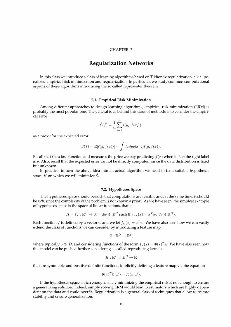
9.3. Maximizing the Margin
Maximizing the margin is a natural approach to select a linear separating rule in the separable case(see Figure 1).
More precisely, consider
βw = mini=1,...,n
βi, βi = yiwT
‖w‖xi, i = 1, . . . , n,
maxw∈RD
βw, subj. to, βw ≥ 0, ‖w‖ = 1.(9.1)
Note that the last constraint is needed to avoid the solution w =∞ (check what happens if you considera solution w and then scale it by a constant k).
In the following, we manipulate the above expression to obtain a problem of the form
minw∈RD
F (w), Aw + c ≥ 0,
where F is convex, A is a matrix and c a vector. These are convex programming problems which can beefficiently solved.
We begin by rewriting problem (9.1) by introducing a dummy variable β = βw to obtain
max(w,β)∈RD+1
β, subj. to, yiwT
‖w‖xi ≥ β;β ≥ 0, ‖w‖ = 1
(we are basically using the definition of minimum as the maximum of the infimal points). We nextwould like to avoid the constraint ‖w‖ = 1. It can be shown that the above problem is equivalent toconsidering
max(w,α)∈RD+1
α
‖w‖, subj. to, yiw
Txi ≥ α;α ≥ 0.
with β = α‖w‖ , where the key idea is that the latter problem is scale invariant. More precisely that we
can always restrict ourselves to ‖w‖ = 1 by appropriately rescaling the solutions. Using again scaleinvariance (check what happens if you consider a solution w and then scale it by a constant (kw, kα)),without loss of generality we can fix α = 1 to obtain
maxw∈RD
1
‖w‖, subj. to, yiw
Txi ≥ 1 , i = 1, . . . , n,
or equivalently
(9.2) minw∈RD
1
2‖w‖2, subj. to, yiw
Txi ≥ 1 , i = 1, . . . , n,
FIGURE 1. Plot of the margin β between the decision function and the nearest samples.

9.6. DEALING WITH AN OFF-SET 29
In the above reasoning we assumed data to be separable; if this is not the case, one could considerslack variables ξ = (ξ1, . . . , ξn) to relax the constraints in the above problem, considering
(9.3) minw∈RD,ξ∈Rn
1
2‖w‖2 + C
n∑
i=1
, subj. to, yiwTxi ≥ 1− ξi, ξi ≥ 0 , i = 1, . . . , n.
9.4. From Max Margin to Tikhonov Regularization
Note that ξi = max0, 1− yiwTxi = |1− yiwTxi|+, for all i = 1, . . . , n. Then if we set λ = 12Cn , we
have that problem (9.3) is equivalent to
minw∈RD,ξ∈Rn
1
n
n∑
i=1
|1− yiwTxi|+ + λ‖w‖2.
9.5. Computations
The derivation of a solution to the SVM problem requires notions of convex optimization, specifi-cally considering so called Lagrangian duality. Indeed, it can be shown that the solution of problem (9.3)is of the form
w =
n∑
i=1
yiαixi
where the coefficients αi for i = 1, . . . , n are given by the solution of the so called dual problem,
(9.4) minα∈Rn
n∑
i=1
αi −1
2
n∑
i,j=1
αiαjyiyjxTi xj , subject to 0 ≤ αi ≤ C, i = 1, . . . , n.
where in particular it can be shown that
αi = 0 =⇒ yiwTxi ≥ 1.
9.6. Dealing with an off-set
Finally, it can be shown that the above reasoning can be generalized to consider an offset, that iswTx+ b, in which case we simply have to add the constraint
n∑
i=1
yiαixi = 0
to the dual problem (9.4).


CHAPTER 10
Dimensionality Reduction
In many practical applications it is of interest to reduce the dimensionality of the data. In particular,this is useful for data visualization, or for investigating the ”effective” dimensionality of the data. Thisproblem is often referred to as dimensionality reduction and can be seen as the problem of defining amap
M : X = RD → Rk, k D,
according to some suitable criterion.
10.1. PCA & Reconstruction
PCA is arguably the most popular dimensionality reduction procedure. It is a data driven procedurethat given an (unsupervised) sample S = (x1, . . . , xn) derives a dimensionality reduction defined by alinear map M . PCA can be derived from several perspectives. Here we provide a geometric/analyticalderivation.
We begin by considering the case where k = 1. We are interested in finding the single most relevantdimension according to some suitable criterion. Recall that, if w ∈ RD with ‖w‖ = 1, then the (orthog-onal) projection of a point x on w is given by (wTx)w. Consider the problem of finding the directionp which allows the best possible average reconstruction of the training set, that is the solution of theproblem
(10.1) minw∈SD−1
1
n
n∑
i=1
‖xi − (wTxi)w‖2,
FIGURE 1. Principal components of a 2D dataset.
31
32 10. DIMENSIONALITY REDUCTION
where SD−1 = w ∈ RD | ‖w‖ = 1 is the sphere in D dimensions. The norm ‖xi − (wTxi)w‖2 measureshow much we lose by projecting x along the direction w, and the solution p to problem (10.1) is calledthe first principal component of the data. A direct computation shows that ‖xi − (wTxi)w‖2 = ‖xi‖ −(wTxi)
2, so that problem (10.1) is equivalent to
(10.2) maxw∈SD−1
1
n
n∑
i=1
(wTxi)2.
This latter observation is useful for two different reasons that the we discuss in the following.
10.2. PCA and Maximum Variance
If the data are centered, that is x = 1nxi = 0, problem (10.2) has the following interpretation: we
look for the direction along which the data have (on average) maximum variance. Indeed, we caninterpret the term (wTx)2 as the variance of x in the direction w. If the data are not centered, to keep thisinterpretation we should replace problem (10.2) with
(10.3) maxw∈SD−1
1
n
n∑
i=1
(wT (xi − x))2,
which corresponds to the original problem on the centered data xc = x − x. In the terms of prob-lem (10.1), it is easy to see that this corresponds to considering
(10.4) minw,b∈SD−1
1
n
n∑
i=1
‖xi − ((wT (xi − b))w + b)‖2.
where ((wT (xi − b))w + b is an affine transformation (rather than an orthogonal projection).
10.3. PCA and Associated Eigenproblem
A simple further manipulation allows to write problem (10.2) as an eigenvalue problem. Indeed,using the symmetry of the inner product we have
1
n
n∑
i=1
(wTxi)2 =
1
n
n∑
i=1
wTxiwTxi =
1
n
n∑
i=1
wTxixTi w = wT (
1
n
n∑
i=1
xixTi )w
so that problem (10.2) can be written as
(10.5) maxw∈SD−1
wTCnw, Cn =1
n
n∑
i=1
xixTi .
We need two observations. First, in matrix notationCn = XTnXn and it is easy to see thatCn is symmetric
and positive semi-definite. If the data are centered, the matrix Cn is the so called covariance matrix.Clearly, the objective function in (10.5) can be written as
wTCnw
wTw
where the latter quantity is the so called Rayleigh quotient. Note that, if Cnu = λu then uTCnuuTu
= λ,since the eigenvector u is normalized. In fact, it is possible to show that the Rayleigh quotient achievesits maximum at a vector which corresponds to the maximum eigenvalue of Cn (the proof of this latterfact uses basic results in linear programming). Then, computing the first principal component of the datais reduced to computing the biggest eigenvalue of the covariance and the corresponding eigenvector.
10.4. Beyond the First Principal Component
Next, we discuss how the above reasoning can be generalized to k > 1, that is more than oneprinciple component. The idea is simply to iterate the above reasoning to describe the input data beyondwhat is allowed by the first principal component. Towards this end, we consider the one-dimensionalprojection which can best reconstruct the residuals
ri = xi − (pTxi)pi,

10.6. KERNEL PCA 33
that is we replace problem (10.1) by
(10.6) minw∈SD−1,w⊥p
1
n
n∑
i=1
‖ri − (wT ri)w‖2.
Note that for all i = 1, . . . , n,
‖ri − (wT ri)w‖2 = ‖ri‖2 − (wT ri)2 = ‖ri‖2 − (wTxi)
2
since w ⊥ p. Then, following the reasoning from (10.1) to (10.2), problem (10.6) can equivalently bewritten as
(10.7) maxw∈SD−1,w⊥p
1
n
n∑
i=1
(wTxi)2 = wTCnw.
Again, we have to minimize the Rayleigh quotient of the covariance matrix. However, when comparedto (10.2), we see that there is the new constraint w ⊥ p. Indeed, it can be proven that the solution ofproblem (10.7) is given by the second eigenvector of Cn, and the corresponding eigenvalue. The proofof this latter fact follows the same line of the one for the first principal component. Clearly, the abovereasoning can be generalized to consider more than two components. The computation of the principalcomponents reduces to the problem of finding the eigenvalues and eigenvectors of Cn. The complexityof this problem is roughly O(kD2), being k the number of components (note that the complexity offorming Cn is O(nD2)).
The principal components can be stacked as rows of a k × D matrix M , and in fact, because of theorthogonality constraint, the matrixM is orthogonal, MMT = I . The dimensionality reduction inducedby PCA is hence linear.
10.5. Singular Value Decomposition
We recall the notion of singular value decomposition of a matrix which allows in some situations toimprove the computations of the principal components, while suggesting a possible way to generalizethe algorithm to consider non linear dimensionality reduction.
Considering the data matrix Xn, its singular value decomposition is given by
Xn = UΣPT .
where U is a n × d orthogonal matrix, P is a D × d orthogonal matrix, Σ is a diagonal matrix suchthat Σi,i =
√λi, i = 1, . . . , d and d ≤ minn,D. The columns of U and the columns of V are called
respectively the left and right singular vectors and the diagonal entries of Σ the singular values. Thesingular value decomposition can be equivalently described by the following equations, for j = 1, . . . , d,
Cnpj = λjpj ,1
nKnuj = λjuj ,
Xnpj =√λjuj ,
1
nXTn uj =
√λjpj ,(10.8)
where Cn = 1nX
TnXn and 1
nKn = 1nXnX
Tn .
If n p the above equations can be used to speed up the computation of the principal components.Indeed, we can consider the following procedure:
(1) form the matrix Kn, which is O(Dn2),(2) find the first k eigenvectors of Kn, which is O(kn2),(3) find the principal components using (10.8), i.e.
(10.9) pj =1√λjXTn uj =
1√λj
n∑
i=1
xiuij , j = 1, . . . , d
where u = (u1, . . . , un), which is again O(knd) if we consider k principal components.
10.6. Kernel PCA
The latter reasoning suggests how to generalize the intuition behind PCA beyond linear dimension-ality reduction by using kernels (or feature maps). Indeed, from equation (10.9) we can see that theprojection of a point x on a principal component p can be written as
(10.10) (M(x))j = xT pj =1√λjxTXT
n uj =1√λj
n∑
i=1
xTxiuij ,

34 10. DIMENSIONALITY REDUCTION
for j = 1, . . . , d.What if we were to map the data using a possibly non linear feature map Φ : X → F , before perform-
ing PCA? If the feature map is finite dimensional, e.g. F = Rp we could simply replace x 7→ Φ(x) andfollow exactly the same reasoning as in the previous sections. Note in particular that equation (10.10)becomes
(10.11) (M(x))j = Φ(x)T pj =1√λj
n∑
i=1
Φ(x)TΦ(xi)uij ,
for j = 1, . . . , d. More generally, one could consider a positive definite kernel K : X ×X → R, in whichcase (10.10) becomes
(10.12) (M(x))j =1√λj
n∑
i=1
K(x, xi)uij ,
for j = 1, . . . , d. Note that in this latter case, while it is not clear how to form Cn, we can still form anddiagonalize Kn, which is in fact the kernel matrix.

CHAPTER 11
Variable Selection
In many practical situations, beyond predictions it is important to obtain interpretable results. In-terpretability is often related to detecting which factors have determined our prediction. We look at thisquestion from the perspective of variable selection.
Consider a linear model
(11.1) fw(x) = wTx =
v∑
i=1
wjxj .
Here we can think of the components xjof an input as of specific measurements: pixel values in the caseof images, dictionary word counting in the case of texts, etc. Given a training set, the goal of variableselection is to detect which variables are important for prediction. The key assumption is that the bestpossible prediction rule is sparse, that is only few of the coefficients in (11.1) are different from zero.
11.1. Subset Selection
A brute force approach would be to consider all the training sets obtained considering all the possi-ble subsets of variables. More precisely we could begin by considering only the training set where weretain the first variable of each input points. Then the one where we retain only the second, and so onand so forth. Next, we could pass to consider a training set with pairs of variables, then triplets etc. Foreach training set one would solve the learning problem and eventually end selecting the variables forwhich the corresponding training set achieves the best performance.
The described approach has an exponential complexity and becomes unfeasible already for rela-tively small D. If we consider the square loss, it can be shown that the corresponding problem could bewritten as
(11.2) minw∈RD
1
n
n∑
i=1
(yi − fw(xi))2 + λ‖w‖0,
where‖w‖0 = |j | wj 6= 0|
is called the `0 norm and counts the number of non zero components in w. In the following we focuson the least squares loss and consider different approaches to find approximate solution to the aboveproblem, namely greedy methods and convex relaxation.
11.2. Greedy Methods: (Orthogonal) Matching Pursuit
Greedy approaches are often considered to find approximate solutions to problem (11.2). This classof approaches to variable selection generally encompasses the following steps:
(1) initialize the residual, the coefficient vector, and the index set,(2) find the variable most correlated with the residual,(3) update the index set to include the index of such variable,(4) update/compute coefficient vector,(5) update residual.
The simplest such procedure is called forward stage-wise regression in statistics and matching pursuit(MP) in signal processing. To describe the procedure we need some notation. Let Xn be the n×D datamatrix and Xj ∈ Rn, j = 1, . . . , D be the columns of Xn. Let Yn ∈ Rn be the output vector. Let r, w, Idenote the residual, the coefficient vector, an index set, respectively.
The MP algorithm starts by initializing the residual r ∈ Rn, the coefficient vector w ∈ RD, and theindex set I ⊆ 1, . . . , D,
r0 = Yn, , w0 = 0, I0 = ∅.
35

36 11. VARIABLE SELECTION
The following procedure is then iterated for i = 1, . . . , T − 1. The variable most correlated with theresidual is given by
k = arg maxj=1,...,D
aj , aj =(rTi−1X
j)2
‖Xj‖2,
where we note that
vj =rTi−1X
j
‖Xj‖2= arg min
v∈R‖ri−1 −Xjv‖2, ‖ri−1 −Xjvj‖2 = ‖ri−1‖2 − aj
The selection rule has then two interpretations. We select the variable such that the projection of theoutput on the corresponding column is larger, or, equivalently, we select the variable such that thecorresponding column best explains the the output vector in a least squares sense.
Then, the index set is updated as Ii = Ii−1 ∪ k, and the coefficients vector is given by
(11.3) wi = wi−1 + wk, wkk = vkek
where ek is the element of the canonical basis in RD, with k-th component different from zero. Finally,the residual is updated
ri = ri−1 −Xwk.A variant of the above procedure, called Orthogonal Matching Pursuit, is also often considered. Thecorresponding iteration is analogous to that of MP, but the coefficient computation (11.3) is replaced by
wi = arg minw∈RD
‖Yn −XnMIiw‖2,
where the D×D matrix MI is such that (MIw)j = wj if j ∈ I and (MIw)j = 0 otherwise. Moreover, theresidual update is replaced by
ri = Yn −Xnwi.
11.3. Convex Relaxation: LASSO & Elastic Net
Another popular approach to find an approximate solution to problem (11.2) is based on a convexrelaxation. Namely, the `0 norm is replaced by the `1 norm,
‖w‖1 =
D∑
j=1
|wj |,
so that, in the case of least squares, problem (11.2) is replaced by
(11.4) minw∈RD
1
n
n∑
i=1
(yi − fw(xi))2 + λ‖w‖1.
The above problem is called LASSO in statistics and Basis Pursuit in signal processing. The objectivefunction defining the corresponding minimization problem is convex but not differentiable. Tools fromnon-smooth convex optimization are needed to find a solution. A simple yet powerful procedure tocompute a solution is based on the so called Iterative Soft Thresholding Algorithm (ISTA). The latter isan iterative procedure where, at each iteration, a non linear soft thresholding operator is applied to agradient step. More precisely, ISTA is defined by the following iteration
w0 = 0, wi = Sλγ(wi−1 −2γ
nXTn (Yn −Xnwi−1)), i = 1, . . . , Tmax
which should be run until a convergence criterion is met, e.g. ‖wi − wi−1‖ ≤ ε, for some precision ε, ora prescribed maximum number of iterations Tmax is reached. To ensure convergence we should choosethe step-size γ = n
2‖XTnXn‖.
Note that the argument of the soft thresholding operator corresponds to a step of gradient descent.Indeed,
2
nXTn (Yn −Xnwi−1)
The soft thresholding operator acts component-wise on a vector w, so that
Sα(u) = ||u| − α|+u
|u|.
A depiction of the sof thresholding is shown in Figure 1.

11.3. CONVEX RELAXATION: LASSO & ELASTIC NET 37
The above expression shows that the coefficients of the solution of problem (11.2) as computed byISTA can be exactly zero: this can be contrasted with Tikhonov regularization where this is hardly thecase.
Indeed, it is possible to see that, on the one hand, while Tikhonov allows to compute a stable solu-tion, in general its solution is not sparse. On the other hand, the solution of LASSO might not be stable.The elastic net algorithm, defined as
(11.5) minw∈RD
1
n
n∑
i=1
(yi − fw(xi))2 + λ(α‖w‖1 + (1− α)‖w‖22), α ∈ [0, 1],
can be seen as hybrid algorithm which is interpolated between Tikhonov and LASSO. The ISTA proce-dure can be adapted to solve the elastic net problem, where the gradient descent step incorporates alsothe derivative of the `2 penalty term. The resulting algorithm is
w0 = 0, wi = Sλαγ((1− λγ(1− α))wi−1 −2γ
nXTn (Yn −Xnwi−1)), i = 1, . . . , Tmax
To ensure convergence, we should choose the step-size γ = n2(‖XTnXn‖+λ(1−α))
.
FIGURE 1. The 1-dimensional soft thresholding operator Sλ with threshold λ.


CHAPTER 12
Density Estimation & Related Problems
Perhaps the most basic statistical inference problem is density estimation, which can be seen as theunsupervised problem of learning a probabilitu density function from random samples.
12.1. Density estimation
Recall that if P is a probability distribution in RD, a probability density function p : RD → [0, 1] is afunction such that for any open set A ⊂∈ RD we have
P (A) =
∫
A
p(x)dx.
Density estimation is the problem of deriving an estimate pn of p given n independent samples x1, . . . , xnof p itself. Below we recall some basic approaches to this problem. In particular, we discuss nonpara-metric methods which avoid explicit parametric assumption on the density to be estimated.
12.1.1. Histogram Estimates. Let’s begin by considering the case D = 1 and assume the density tobe zero outside of [0, 1]. An histogram estimate is defined by a partition of the interval [0, 1] in N = 1/hintervals (bins) of lengths h. If we denote the bins by B1, . . . , BN , for all x ∈ R the histogram estimate isdefined by
pn(x) =
N∑
j=1
Njh
1Ix∈Bj (x),
where
Nj =1
n
∑
i=1
1Ixi∈Bj (xi).
The estimator assign to a point x belonging to a binBj a local density estimate given by the ratio betweenthe fraction of point in the interval and the size of the interval.
The estimator can be naturally generalized to higher dimensions at least as long as the density iszero outside of [0, 1]D. In this case, N = 1/hD bins are taken to be cubes with edge h. The correspondinghistogram estimator is given by
pn(x) =
N∑
j=1
NjhD
1Ix∈Bj (x),
with Nj defined as above. Histograms are probably the simplest and most common density estimators.The above construction is based on a partition of the data space in bins. This latter operation is the mainchallenge to use this kind of techniques, especially in high dimensions.
12.1.2. Kernel Density Estimator. Kernel Density Estimators (KDE) are also a very classical ap-proach to density estimation. They are defined via a smoothing a kernel, which is a function K : R→ Rsuch that ∫
K(x)dx = 1,
∫xK(x)dx = 0,
∫x2K(x)dx <∞.
For D = 1, examples of commonly used kernels include the box kernel
K(x) =1
21I[−1,1](0),
and the Gaussian
K(x) =1√2πex
2/2.
39

40 12. DENSITY ESTIMATION & RELATED PROBLEMS
Kernel for higher dimension can be derived considering eitherD∏
j=1
K(xj) or K(‖x‖) .
Considering this latter choice, for all x ∈ RD the kernel density estimator is defined by
pn(x) =1
n
n∑
i=1
1
h
D
K
(‖x− xi‖
h
)
where again h is a scale parameter, also called bandwith. A kernel density estimator can be thought ofas placing a fraction 1/n of the total mass at each data point and the final estimator can be seen as theaverage of the kernels centered over the data points.
12.1.3. Parameter Tuning. Both the above estimators depend crucially on the choice of a “scale”parameter h. Since the density estimation problem is unsupervised it is natural to ask:
(1) whether a form of Bias Variance trade-off can be seen to underlie the parameter choice;(2) whether a form of cross validation can be used in practice.
This is indeed the case and we next sketch some basic ideas. We omit discussing the Bias-Variancetrade-off and describe instead a cross validation procedure considering a basic hold-out approach.
In the following, we explicitly indicate the dependence of the estimator on the scale h writing pn,h.Ideally, the scale h should be chosen to minimize a measure of the discrepancy between pn,h and p, forexample
D(h) =
∫(pn,h(x)− p(x))2dx.
However, this cannot be done directly since p is not known. An idea to derive an empirical criterion canbe seen further developing the above quantity into
D(h) =
∫(p(x))2dx+
∫(pn,h(x))2dx− 2
∫pn,h(x)p(x)dx.
Clearly the first term in the above expression does not depend on h. If we split the data in two (say)equal sets then the idea is to use the first half to define pn
2 ,hand the second holdout set to define the
following empirical estimate
D(h) ≈ Dn2
(h) =
∫(pn
2 ,h(x))2dx− 2
1
n
n∑
i=1
pn2 ,h
(xi).
The latter term can be computed from data for any estimator, while the other term might requires somefurther approximations to compute the integral.
The scale parameter can then be chosen minimizing Dn2
(h) among M possible choiches h1, . . . , hMWe remark that, importantly, the estimator pn
2 ,hand the empirical discrepancyDn
2(h) are computed
over distinct data splits. We also note that the described procedure can be easily extended to considermultiple splits (V-fold cross validation and leave one out).
12.2. Applications of Density Estimation to Other Problems
Density estimation can be seen a the starting point of solving other problems.A first example are supervised problems, where density estimation can be directly applied to esti-
mate the conditional density p(y|x). We next discuss two further examples.
12.2.1. Support Estimation & Anomaly Detection. The support of a probability distribution is de-fined as the smallest set S such that P (S) = 1 or equivalently if p is the probability density functioncorrespnding to P ,
S = x ∈ RD | p(x) > 0.Clearly given a density estimate pn an empirical estimate of the support can be defined by
Sn = x ∈ RD | pn(x) > 0,or rather by
Sn,τ = x ∈ RD | pn(x) > τ,In the latter expression a threshold parameter τ was added, the intuition being that the τ accounts forthe accuracy of empirical density estimates and should be a decreasing function of n.

12.2. APPLICATIONS OF DENSITY ESTIMATION TO OTHER PROBLEMS 41
The problem of support of estimation is closely related to the problem called anomaly, or novelty,detection. As they name suggest this is the problem of determining whether a data point belong to agiven distribution. To some extent this can be seen as a classification problem where one of the two classis much more numerous than other and only example of this larger class are given a training time. Apossible approach is to use these data points to derive a density estimate and deciding whether a pointis an anomaly/novelty by checking whether it belongs to Sn,τ . In this case, the threshold determinesthe fraction of points that will be considered to be anomalies/novelties.
12.2.2. Level Set Clustering. The problem of clustering is to partition the data space in distinct sets,called cluster. Given a probability density function one way to make this precise to define the cluster tobe the connected components of the support S.
Given n independent samples x1, . . . , xn from p this suggest that cluster can be defined based ondata computing the connected components of Sn, or rather Sn,τ .
This latter task is straightforward in one dimension, but requires some care in general. A possi-ble approach is to build a graph Gn with vertices in the points x1, . . . , xm ∈ Sn,τ and edges given by1I‖xi−xj‖≤ε for all i, j = 1, . . . ,M . Here ε is a threshold which could be chosen for example to be thesame as the scale h of the density estimator. Given the graph Gn the clusters are defined as the con-nected components of the graph.


CHAPTER 13
Clustering Algorithms
Clustering is one of the most fundamental unsupervised learning problem. Yet it lacks a clear def-inition and different estimation/algorithmic approaches are informed by different definitions. Ratherthan attempting an exact definition here we informally refer to the clustering problem as the problem oflearning a partition of the data space from a given data-set x1, . . . , xn. The elements of the partition arethe clusters.
Next we provide a brief description of three main approaches, K-Means, hierarchical clustering andspectral clustering.
13.1. K-Means
The basic idea of K-means is to define clusters by a set of centers (means) considering the corre-sponding Voronoi partition. Recall that, given a set of K means m1, . . . ,mK ∈ RD, the elements of thecorresponding Voronoi partition are the clusters defined by
Cj = x ∈ RD | ‖x−mj‖ ≤ ‖x−mi‖ , ∀i = 1, . . . ,K, i 6= j,
for j = 1, . . . ,K (with ties broken arbitrarily).Since each cluster is identified with a center, the clustering problem is reduced in to K-Means to
finding the K means solving the following minimization problem
minm1∈RD,...,mK∈RD
n∑
i=1
minj=1,...,K
‖xi −mj‖2 .
The above problem is nonconvex and in general can be hard to solve. We next describe some commonapproaches to find approximate solutions.
13.1.1. Lloyd’s Algorithm. Lloyd’s algorithm is the classical procedure to find an approximate so-lutions to the k-means problems and essentially corresponds to an alternating minimization approach.Indeed, the K-means minimization problem requires to search for a set of means and also for the bestmean for each point. The idea is to alternate these two search steps as follows.
(1) The algorithm is initialized with a given set of means.(2) Then the inner minimization is solved, which is typically referred to as the assignment steps,
since each training point is assigned to one of the means, hence to a cluster.(3) The outer minimization is then performed. The minimization over each mean can be done
separately and corresponds to the computation of the center of mass of each cluster. This stepis typically referred to as the updated step.
(4) Step 2 and 3 are repeated until a convergence criterion is met. Typically if the value of theobjective function does not decrease or decrease only slightly.
Lloyd’s algorithm is not ensured to a converge to a global solution. However it can be be shownto terminate in a finite number of steps and to always decrease or at least not increase the objectivefunction. As in all non convex problems the effect of initialization is critical. We next discuss a fast yetpowerful choice.
13.1.2. K-Means ++. K-means ++ is a simple procedure to obtain an set of means that are likely tobe widespread in the data-set.
The following are the main steps of the algorithm.(1) The first mean is chosen uniformly at random from the training set and included in a set M .(2) Then, the distance of each of the remaining training points to M is computed,
Di = minx∈M‖x− xi‖ .
43

44 13. CLUSTERING ALGORITHMS
(3) A new mean is sampled with probability proportional to
pi =D2i∑
iD2i
(4) The set M is updated to include to the new mean and steps 2 and 3 are repeated until K meansare sampled.
K-means++ provides a set of centers which can be shown to be close in expectation to a global solutionand is typically refined using Lloyd’s algorithm.
13.2. Hierarchical Clustering
Hierarchical clustering is a form of agglomerative clustering, thus called since a sequence of parti-tions (clusterings) is recursively build agglomerating points first and then clusters. The key ingredientof this class of algorithms is a distance function among points as well as distance between sets (clusters).Considering a Euclidean distance several examples of distances between sets are given below.
• Single Linkaged(A,B) = min
x∈A,x′∈B‖x− x′‖
• Average Linkage
d(A,B) =1
]A ]B
∑
x∈A,x′∈B‖x− x′‖
• Complete Linkaged(A,B) = max
x∈A,x′∈B‖x− x′‖
where A,B are subsets of RD (in particular single points). For each one of the above choices the algo-rithm proceed as follows:
(1) first each training point is defined as (the center of) a cluster, that is
Ci = xi, i = 1, . . .
to provide a clustering Tn = C1, . . . , Cn.(2) Then, the cluster Ci, Cj for which d(Ci, Cj) is minimal, according to one of the above distance
function, are found and fused into a new cluster Ci ∪ Cj . The corresponding clustering isdenoted by Tn−1.
(3) The latter step repeated until there is only one cluster and the sequence of clustering Tn, . . . , T1
is returned as output.Hierarchical clustering provides not a single clustering but a family of clustering that can repre-
sented as a tree, called a dendogram. The different clustering are obtained considering different cut ofthe tree. Clusters obtained using single linkage tend to be elongated whereas those obtained by usingcomplete linkage are more isotropic. Average linkage seems to provide results which are between thesetwo opposite behaviors
13.3. Spectral Clustering
The basic idea is to associate a weighted graph G = (V,E) to the data, where there is one vertex perpoint and a a symmetric matrix W of positive weights is given, or simply and adjacnecy matrix. Such aconstruction can be done in various way. The simplest example is the so called ε-neighborhood graph.Here all points with distance smaller than ε are connected, i.e.
Wi,j = 1I‖xi−xj‖≤ε.
In this, case the graph is typically sparse and unweighted. Another possibility is to consider
Wi,j = e−‖xi−xj‖2/2σ2
,
in which case the graph is fully connected (albeit faraway points will have small weight).The key quantity is the so called graph Laplacian associate to the graph, defined as
L = D −W,

13.3. SPECTRAL CLUSTERING 45
where D is the diagonal matrix with entries Di,i =∑nj=1Wi,j . The graph Laplacian or rather its spectral
properties yield direct information on the geometry of the underlying graph. Clearly L is a symmetricand by direct computation it is possible to see that it is also positive definite, since for all v ∈ Rm it holds,
v>Lv =1
2
n∑
j=1
n∑
i=1
Wi,j(vi − vj)2 ≥ 0.
The following key properties can be proved:• the number k of eigenvectors v1, . . . , vk with eigenvalue 0 can be shown to be equal to the
number of connected components in the graph.• The eigenvectors v1, . . . , vk are orthogonal and each one is constant over one of the connected
components.The proof of the above two facts is quite elementary but outside our scopes. The above result can bedirectly applied to cluster the data, by considering the connect components of thew graph and pointsdefining the corresponding vertices as clusters. We end noting mentioning that there are other possibleway to use the eigenvectors of L to define a clustering. The most common way to is to first com-pute eigenvectors v1, . . . , vk, that can be viewed as the rows of a k by n matrix V . The, n the columnsV 1, . . . , V n of this matrix are seen as points and clustered typically using K-means. While the describedprocedure is relatively simple, its justification requires a longer treatment.


CHAPTER 14
Graph Regularization
We next discuss the problem of predicting the value of a function on a graph and discuss the con-nection to transductive and semisupervised learning.
14.1. Graph Labelling via Regularization
Consider an undirected acyclic graph G = (V,E) with m vertices and let W be the corresponding mby m adjacency matrix, or more a generally a symmetric matrix of positive weights.
In the problem we consider, a subset of n < m vertices is given labels y1, . . . , yn ∈ Y , and the goal isto assign a label to each of the other vertices. Here the labels can be binary Y = −1, 1 or real valuedY = R.
14.1.1. Graph Labelling as Supervised Learning. This problem can be compared to a supervisedproblem on a discrete input space. The idea is to identify each vertex with an index in the range [m] =1, . . . ,m and the latter with the input space X . Then each function f : [m] → Y can be viewed as avector in Rm with entries f(i). If we assume, without loss of generality, the first n vertices to be labelled,than the problem is to find an unknown function f∗ given a training set (1, y1), . . . , (n, yn), but alsoknowledge of the rest of the vertices/weights of the graph.
Note that in general the labelled vertices might, or might not, be chosen at random and also thecorresponding labels might or might not be noisy/probabilistic. In the simplest case for all i = 1, . . . , nwe have yi = f∗(i) where f∗ is the function to be estimated. This is the situation we consider next.
14.1.2. Regularization. To derive a learning scheme, a basic idea is to assume the function to beestimated to be sufficiently smooth. A possible way to make this precise is to require nearby verticesto have similar function values, an intuition that can be used to consider the following functional R :Rm → [0,∞),
R(f) =1
2
m∑
i,j=1
Wi,j(f(i)− f(j))2,
for all f ∈ Rm, that is f : [m] → R. In turn the above functional can be used to derive the followingestimation scheme
minf∈Rm
R(f), subject to f(i) = yi, i = 1, . . . , n.
The interpretation is that we are looking for a function on the graph such that,
• The function has the correct values yi = f∗(i) on the labelled vertices, and• nearby vertices should have similar function values.
14.1.3. Graph Regularization Computations. It useful to rewrite the above problem in vectorialform to use tools from linear algebra.
First note that, if we denote by D be the diagonal matrix with entries Di,i =∑mj=1Wi,j , and L =
D −W thenR(f) = f>Lf.
We need some more notation. It is useful to write f = (fn, fu) where fn ∈ Rn and fu ∈ Ru withu = m− n. Also it useful to write L in four block
L = (Ln, Lnu;Lun, Lu),
where Ln is n by n, Lu is u by u and Lnu, Lun are n by u and u by n, respectively.Finally, let Yn ∈ Rn bethe label vector.
47

48 14. GRAPH REGULARIZATION
Then, considering the different blocks we can write,
R(f) = f>Lf
= f>n Lnfn + f>n Lnufu + f>u Lunfn + f>u Lufu
= f>n Lnfn + 2f>u Lunfn + f>u Lufu.
If we impose the constraint fn = Yn, then we can take, and set to zero, the gradient with respect to theremaining unknown variables, that is fu, to obtain
∇fuR(f) = 2LunYn + 2Lufu = 0
which implies thatfu = (Lu)−1LunYn
assuming Lu to be invertible. From a computational point of view graph regularization reduces to thesolution of a linear system.
14.1.4. Considering Noisy Labels. In the case labels are affected by noise the natural approach isto change the formulation in (??) by relaxing the constraint and considering,
minf∈Rm
R(f), subject to ‖fn − Yn‖2 ≤ γ,
where γ is a parameter to be determined. Alternatively the following formulation can be considered.
minf∈Rm
R(f) + λ ‖fn − Yn‖2 ,
where the tuning parameter now is λ. The computation in this latter case can be deduced extending theapproach in the noiseless case.
14.2. Transductive and Semi-Supervised Learning
We end discussing the connection between graph regularization and transductive and semi-supervisedlearning. These latter problems are similar.
• In transductive learning, there is set of m input points x1, . . . , xn ∈ RD of which only the firstn have labels y1, . . . , yn ∈ R. The goal is to assign labels to the remaining u = m− n unlabelledpoints.
• In semi-supervised learning, the problem is the classical supervised statistical learning prob-lem, but extra unlabelled data are provided at training time. The goal is to perform well on allpossible future data given a training set (x1, y1), . . . , (xn, yn), the difference being that now alsoa set of unlabelled points x1, . . . , xu is given.
From a practical point of view a transductive algorithm can used for semi-supervised learning by re-traininig/testing for any new unlabelled point.
14.2.1. From Graph Labelling to Semi-Supervised Learning. The basic idea is to use the graphregularization on a graph built from data with the same procedures introduced for spectral clustering.
A possibly weighted graph G = (V,E) is built from the data, considering one vertex per pointand edges/weights given by a data driven symmetric matrix W . The simplest example is the so calledε-neighborhood graph. Here all points with distance smaller than ε are connected, i.e.
Wi,j = 1I‖xi−xj‖≤ε.
In this, case the graph is typically sparse and unweighted. Another possibility is to consider
Wi,j = e−‖xi−xj‖2/2σ2
,
in which case the graph is fully connected (albeit faraway points will have small weight). Vertices in-herit the labels (when available) from the corresponding input points. Function over the labelled andunlabeled points can be identified with function over the vertices and the graph regularization proce-dure can be directly applied.Note that for semi-supervised learning the graph should be updated and a solution recomputed every-time a new unlabelled point is added.

CHAPTER 15
Bayesian Learning
The point of view taken thus far is to try whenever possible to estimate only the quantity of interestrather than the underlying probability distribution, and iny case trying to make as little assumptionsas possible on the latter. This perspective is in contrast with Bayesian approaches where probabilitydistribution are the central objects of interest. We next provide some basic idea for this class of methods.
15.1. Maximum Likelihood Estimation
Maximum Likelihood Estimation (MLE) is one of the most classical estimation principles. The basicidea of maximum likelihood estimation is to derive the assume a parametric model for the unknown thedistribution and then estimate the parameter which mostly likely generated the data.
15.2. Maximum Likelihood for Density Estimation
Consider the problem of estimating a density function p on R, from independent samples x1, . . . , xn.In contrast to nonparametric approaches, here we make explicit parametric assumptions on the uknowndistribution. In particular, we begin assuming p to be a standard Gaussian, so that the problem reducesto the estimation of the mean. In the following we denote by pµ the density to explicitly indicate thedependence on the unknown mean.
Since the data are independent, their joint distribution, called likelihood, is the product of the indi-vidual distributions
n∏
i=1
pµ(xi) =
n∏
i=1
1√2πe−|xi−µ|
2
= e− 1√
2π
∑ni=1 |xi−µ|2
where we used the Gaussian assumption in the last equalities. The log-likelihood is simply the logarithmof the above quantity
log
n∏
i=1
pµ(xi) ∝ −n∑
i=1
|xi − µ|2.
The idea is then to choose the value of the mean that maximize the likelihood (and hence the jointprobability of observing the given data). We add several remarks.
• In the above example, it is straightforward to see that the best MLE of the mean is
µn =1
n
n∑
i=1
xi.
• The above example can be extended to consider more unknown parameters, for example boththe mean and the variance. In this case, the likelihood is a multivariate function (a function ofmany variables).
• The above example can also be easily generalized to multiple dimensions considering a multi-variate Gaussian
N(µ, I) = Ce−‖xi−µ‖2
where C is a normalizing constant. In this case, the log-likelihood is proportional to
−n∑
i=1
‖xi − µ‖2 .
• Finally, the above example can generalized to parametric assumptions pθ other than Gaussian,where θ is a vector of unknown parameters. In this case the likelihood is a function of θ.
49
50 15. BAYESIAN LEARNING
15.3. Maximum Likelihood for Linear Regression
The above approach can be applied to linear regression. Consider the regression model
yi = w>xi + εi, i = 1, . . . , n,
and assume for all i = 1, . . . , n, that εi are independent samples of a Gaussian N(0, σ2). Here thevariance σ > 0 can be seen as a noise level. The goal is to estimate the unknown coefficient vector w∗,given (x1y1), . . . , (xn, yn).
Following a MLE approach, for all i = 1, . . . , n, we are going to consider the conditional distribution
p(yi, |xi;w)
given by the Gaussian N(w>xi, σ2) = Ce−1
2σ2 |w>xi−yi|2 , where C is a normalizing constant. Then,because of independence,
p(y1, . . . , yn|w∗, x1, . . . , xn;w) = −n∏
i=1
Ce−|w>xi−yi|
2
2σ2 = C ′e−1
2σ2
∑ni=1 |w>xi−yi|2
where C ′ is a normalizing constant. Then the likelihood is proportional to
− 1
σ2
n∑
i=1
|w>xi − yi|2
and we see that maximizing the likelihood reduces to the least squares.In other words, least squares can be derived from a MLE approach considering a linear regression
model under a Gaussian noise model.
15.4. Prior and Posterior
The basic idea of Bayesian estimation is that the parameter of interest follow a prior distributionreflecting our prior knowledge/beliefs on the problem. The idea is then to derive the so called posteriordistribution, obtained conditioning the prior to the observed data. The basic tool is the Bayes rule,which, given two random variables U, V , in its simplest form, is expressed by the equality
P (U |V ) =P (V |U)P (U)
P (V ).
15.4.1. Posterior for Linear Regression. We illustrate the above idea in the case of linear regression.In this case, a classic prior is expressed by the assumption that the unknown coefficient vector w isdistributed according to a standard multivariate Gaussian N(0, I).
The idea is to apply the Bayes rule to the data and the coefficient vectorw seen as random quantities.More precisely we have
P (w | y1, . . . , yn;x1, . . . , xn) = P (y1,...,yn;x1,...,xn | w)P (w)P (y1,...,yn;x1,...,xn)
= P (y1,...,yn | x1,...,xn;w)P (w)P (y1,...,yn|x1,...,xn) ,
or using a more compact vector notation
P (w | Xn, Yn) =P (Yn | Xn, w)P (W )
P (Yn|Xn, ),
where Xn denotes the n by D inputs matrix and Yn the n dimensional vector of corresponding outputs.Several comments can be made.
• The above expression can be interpreted as determining how our prior beliefs, P (w), are up-dated once we observe the data, P (w|y1, . . . , yn;x1, . . . , xn). The latter quantity is called poste-rior probability.
• From the Bayes rule we have that the posterior depends on the product of likelihood and theprior divided by the, so called, marginal likelihood.
• The marginal likelihood is only a normalizing factor since it does not depend on w.Given the Gaussian assumptions on the noise and coefficient vector, the posterior expression can begiven explicitly, as we discuss next.
From the above discussion we have that
P (w | Xn, Yn) ∝ P (Yn | Xn, w)P (W )
15.5. BEYOND LINEAR REGRESSION 51
The first term in the right end side can be identified with the likelihood
P (Yn | Xn, w) = Ce−∑ni=1‖wT xi−yi‖2
2σ2 ,
whereas the second term is the priorP (w) = C ′e−‖w‖
2
,
for suitable normalizing constants C,C ′. This means that the posterior is given up to a normalizingconstant by
e−1
2σ2
∑ni=1 |wT xi−yi|2e−‖w‖
2
= e−( 12σ2
∑ni=1 |wT xi−yi|2+‖w‖2).
In words, the posterior is given by the product of two Gaussian distributions and a possible parameterestimate is given by computing its maximum (which is also equal to its mean). This parameter estimateis called Maximum A Posteriori (MAP) and is given by the solution of the problem
maxw∈RD
e−( 12σ2
∑ni=1 |wT xi−yi|2+‖w‖2).
As in the case of the MLE for linear regression with Gaussian noise model, also the MAP estimatescorresponding to the Gaussian prior provides an interesting connection. Indeed the above problem isequivalent to
minw∈RD
1
2σ2
n∑
i=1
|wTxi − yi|2 + ‖w‖2 .
In other words ridge regression can be derived as the MAP estimate for linear regression under a Gauss-ian prior and Gaussian noise model. In this case the regularization parameter is determined by the noiselevel.
Beyond the maximum (or mean) parameter, the interest of having an explicit expression for theposterior is that other moments can be computed, for example the variance of the parameter estimate.We won’t develop further these computations, but only point out how the possibility of estimating thishigher order information is a hall-mark of Bayesian approaches, where it is referred to as uncertaintyquantification.
15.5. Beyond Linear Regression
The above ideas can be extended in a number of different ways.Non-linear parametric regression. It is straightforward to see that the above reasoning and calcula-
tions extend to the case where we consider a regression model
yi =
p∑
j=1
wj∗φj(xi) + εi, i = 1, . . . , n,
for some set of p features φj : RD → R, j = 1, . . . , p. Indeed, all the above estimates hold simplyreplacing xi by xi = (φ1(xi), . . . , φp(xi)) for all i = 1, . . . , n.
Non-linear nonparametric regression:Gaussian Processes. It is also possible to consider the exten-sion of the above reasoning to an infinite set of features essentially deriving a parallel of kernel methodsfrom a Bayesian perspective. This derivation, based on Gaussian processes, is outside the scope of ourpresentation.
From regression to classification. Finally the above reasoning can also be considered in the case ofclassification. Following the Bayesian ansatz a suitable probabilistic model needs be specified in thiscase since the regression model with Gaussian noise is meaningless in this case. While this is indeedpossible, in general the corresponding computations are more involved. Also this topic left out fromthis presentation.


CHAPTER 16
Neural Networks
So far we have considered that model of the form
fw(x) = w>Φ(x)
and two steps learning scheme with
• supervised learning of w,• expert design or unsupervised learning of the data representation/feature map Φ.
The basic intuition is that the data representation/feature map Φ maps the data in a new format bettersuited for further processing. A key observation is that in model of the above form, non linear functionsare parameterized linearly and nonlinearity is taken car of by feature map.
Neural network are an alternative way to derive non linear function, by allowing a non linear pa-rameterization. The simplest form of neural network corresponds to consider
Φ(x) = σ(Wx)
and
fw,W (x) = w>σ(Wx)
where B is a u by D matrix, and σ a non linear map acting component-wise, that is
σ(Wx) = (σ(W>1 x), . . . , σ(W>u x))
denoting by Wi, i = 1, . . . , u the rows of W . Examples of non-linearities include:
• sigmoid s(α) = 1/(1 + e−α)t,• hyperbolic tangent s(α) = (eα − e−α)/(eα + e−α),• ReLU s(α) = |α|+ (aka ramp, hinge),• Softplus s(α) = log(1 + eα).
where α ∈ R.
Some jargoon is typically used to denominate the different elements of a NN.
• The first set of parameters W is called a (hidden) layer.• The number u of rows in W is the number of hidden units.• The non linearity σ is called activation function, from an analogy to biological networks, as we
describe next.
Biological interpretation. The above functional model can be given a biological interpretation. Thesimplest model of a neuron is that of a unit that computes an inner product with a vector, e.g. a columnof a weight matrix W , and then applies a non-linearity σ, which is the neuron activation function.
53

54 16. NEURAL NETWORKS
Hence, the computation in a neuron is given by
σ(
D∑
j=1
W ji x
j),
where x is an input divided in its components (x1, . . . , xD). The output of each of these neurons is thengiven in input to another neuron computing the inner product with a weight vector w,
fw,W (x) =
u∑
i=1
wiσ(
D∑
j=1
W ji x
j).
Note that, in this latter case a non linearity can also be applied.
x3x2x1
W 1j
W 2j
W 3j
W>j x =
3X
t=1
W tj xt
hi, i am a neuronLearning data representation. Another possible way to look at neural networks is as providing an
approach to learn a data representation. The first step towards learning a representation is to define aparameterization that can be estimated from data. The simplest parameterization, i.e. assuming Φ to belinear, i.e. Φ(x) = Wx, provides linear functions
fw,W (x) = w>(Wx)
hence is too simple. From this perspective neural networks can be seen to provide the simplest param-eterization leading to nonlinear functions, since a simple component-wise non linearity is considered.
Both the above perspectives suggest possible extensions of the above model. In biological networksmultiple neurons are organized in a hierarchical fashion. From a data representation point of composingmultiple stages comprising linear transform and non linearities hold the promise to provide richer datarepresentations. Developing these idea leads to deep neural networks.
16.1. Deep Neural Networks
The basic idea is to compose multiple feature map of the above form. For example, consider twohidden layers Φ1 : RD → Ru1 ,
Φ1(x) = σ(W1x)
and Φ2 : Ru1 → Ru2 ,Φ2(x) = σ(W2x).
can be composed to obtainΦ2 Φ1(x) = σ(W2σ(W1x)).
The output of neurons at one layer are given as input to the next. The above can be seen as a newcomposite representation and can be used to derive a function
fw,W1,W2(x) = w>Φ2 Φ1(x) = w>σ(W2σ(W1x)).
Clearly, the above reasoning can be recursively applied, at the expanse of a heavier notation. Fori = 1, . . . , L, let Wi be ui−1 times ui matrices, where ui ∈ N and u0 = D. Then for i = 1, . . . , L letΦi(z) = σ(Wiz), where z ∈ Rui−1 and consider
Φ(Wi)i(x) = ΦL Φ1(x) = σ(WL . . . σ(W1x))))).
A function is then obtained considering
fw,(Wi)i(x) = w>Φ(Wi)i(x)

16.2. ESTIMATION AND COMPUTATIONS IN DNN 55
and depends on all the parameters at every layer.
x3x2x1
W 1j
W 2j
W 3j
W>j x =
3X
t=1
W tj xt
16.2. Estimation and Computations in DNN
The basic ideas to estimate the parameters of a DNN is to consider the minimization of the empiricalerror as measured by a given loss function, e.g. the logistic or the least squares loss. In this latter case,the problem can be written as
minw,WEn(w,W ), En(w,W ) =
n∑
i=1
(yi − f(w,W )(xi)))2.
where to ease the exposition we considered only one hidden layer. Further penalties or constrainedon the weights can be considered, e.g. assuming ‖w‖2 ≤ 1 and ‖W‖@ ≤ 1. In this latter expression,different matrix norm can be considered, the simplest case being the squared Frobenious norm given byTrace(WTW ).
From a computational point of view the above problem is tricky, since the resulting minimizationproblem is smooth but not convex. Gradient descent techniques can be applied, however no conver-gence guarantees can be given.
Convex vs. Nonconvex Optimization
Unique optimum: global/local. Multiple local optima
16.2.1. Gradient Descent and Backpropagation. An approximate minimizer is computed via thefollowing gradient method
wt+1j = wtj − γt
∂En∂wj
(wt,W t)
W t+1j,k = W t
j,k − γt∂En∂Wj,k
(wt+1,W t)
where the step-size (γt)t is often called learning rate.Direct computations show that:
∂En∂wj
(w,W ) = −2
n∑
i=1
(yi − f(w,W )(xi)))︸ ︷︷ ︸∆j,i
hj,i
∂En∂Wj,k
(w,W ) = −2
n∑
i=1
(yi − f(w,W )(xi)))wjσ′(w>j x)
︸ ︷︷ ︸ηi,k
xki
ηi,k = ∆j,icjσ′(w>j x)

56 16. NEURAL NETWORKS
Using above equations, the updates are performed in two steps:• Forward pass compute function values keeping weights fixed,• Backward pass compute errors and propagate• Hence the weights are updated.
16.3. Convolutional Neural Networks
A convolutional neural network (CNN) can be seen as a neural networks with more complex lin-ear and non linear operations. The linearity is now a convolution. Recall that given a vector t, theconvolution between w and x is denote by t ∗ x and given by
(t ∗ x)j =
D∑
i=1
tj−ixi.
Convolution returns a vector with components given by the inner product between x and shifted versionof the vector w. As seen above the basic linear operation in a neural network is
σ(t>x).
In CNN the inner product is replaced with a convolution and the non linearity is a block operation thataggregates all values in a single one, for examples a max,
maxj=1,...,D
(t ∗ x)j .
At each layer a representation is built considering the above operation for multiple vectors t1, . . . , tu.

CHAPTER 17
A Glimpse Beyond The Fence
We next try to give a brief overview of 1) topics in machine learning that we have not touched upon,2) some of the current and future challenges in machine learning.
17.1. Different Kinds of Data
Different machine learning approaches arise to deal with different kinds of input and output. Re-call that the input/output pairs are assumed to belong to an input space X and an output space Y ,respectively. We call Z = X × Y the data space. We list a few examples of input and output spaces.
• Euclidean/Vector Spaces. Perhaps the simples example, covering many practical situations, isX = Rd, d ∈ N.
• Probability distributions. We could set X = x ∈ Rd+ :∑dj=1 x
j = 1, d ∈ N, and view elementsof the space as probability distributions on a finite set Ω of dimension d. More generally givenany probability space Ω we can view X as the space of probability distribution on Ω.• Strings/Words. Given an alphabet Σ of symbols (letters), one could consider X = Σp, p ∈ N,
the (finite) space of strings (words) of p letters.• Graphs. We can view X as collection of graphs, i.e. X = .
Clearly more exotic examples can be constructed considering compositions of the above examples, forexample X = Rd × Σp, d, p ∈ N etc.
Next, we discuss different choices of the output space and see how they often correspond to prob-lems with different names.
• Regression, Y = R.• Binary classification, Y = −1, 1. Where we note that here we could have taken Y = 0, 1–
as well as any other pair of distinct numeric values.• Multivariate regression, Y = RT , T ∈ N, each output is a vector.• Functional regression, Y is a Hilbert space, for example each output is a function.• Multi-category classification, Y = 1, 2, . . . , T, T ∈ N, the output is one of T categories.• Multilabel, Y = 21,2,...,T, T ∈ N, each output is any subset of T categories.
An interesting case is that of so called multitask learning. Here Z = (X1, Y1) × (X2, Y2) × · · · ×(XT , YT )) and the training set is is S = (S1, S2, . . . , ST ). We can view each data space/training set ascorresponding to different, yet related, tasks. In full generality, input/output spaces and data cardinalitycan be different.
17.2. Data and Sampling Models
The standard data model we consider is a training set as an i.i.d. sample from a distribution p onthe data space Z.
• Semisupervised, the more general situation where unlabelled data Su are available togetherwith the labelled data S.• Transductive, related to the above setting, unlabelled data Su are available together with the
labelled data and the goal is to predict the label of the unlabeled data set Su.• Online/Dynamic Learning, the data are not i.i.d. The samples can be dependent, can come
from varying distribution, or both.
17.3. Learning Approaches
• Online/Incremental• Randomized• Distributed
57

58 17. A GLIMPSE BEYOND THE FENCE
• Online/Dynamic Learning, the data are not i.i.d. The samples can be dependent, the samplescan come from varying distribution or both.
• Active• Reinforcement Learning
17.4. Some Current and Future Challenges in Machine Learning
Challenges1← Data Size→∞
17.4.1. Big Data? Recent times have seen the development of technologies for gathering data-setof unprecedented size and complexity both in natural science and technology. On the one hand thishas opened novel opportunities (e.g. online teaching), on the other had it has posed new challenges.In particular, the necessity has emerged to develop learning techniques capable to leverage predefinedbudgets and requisites in terms of
• Computations,• Communications,• Privacy.
17.4.2. Or Small Data? One of the most evident differences between biological and artificial intel-ligence is the astounding ability of humans to generalize from limited supervised data. Indeed, whileimpressive, current artificial intelligent systems based on supervised learning require huge amounts ofhumanly annotated data.
• Unsupervised learning of data representation• Learning under weak supervision.• Learning and exploiting structure among learning tasks.
APPENDIX A
Mathematical Tools
These notes present a brief summary of some of the basic definitions from calculus that we will needin this class. Throughout these notes, we assume that we are working with the base field R.
A.1. Structures on Vector Spaces
A vector space V is a set with a linear structure. This means we can add elements of the vectorspace or multiply elements by scalars (real numbers) to obtain another element. A familiar exampleof a vector space is Rn. Given x = (x1, . . . , xn) and y = (y1, . . . , yn) in Rn, we can form a new vectorx+ y = (x1 + y1, . . . , xn + yn) ∈ Rn. Similarly, given r ∈ R, we can form rx = (rx1, . . . , rxn) ∈ Rn.
Every vector space has a basis. A subset B = v1, . . . , vn of V is called a basis if every vector v ∈ Vcan be expressed uniquely as a linear combination v = c1v1 + · · ·+ cmvm for some constants c1, . . . , cm ∈R. The cardinality (number of elements) of V is called the dimension of V . This notion of dimensionis well defined because while there is no canonical way to choose a basis, all bases of V have the samecardinality. For example, the standard basis on Rn is e1 = (1, 0, . . . , 0), e2 = (0, 1, 0, . . . , 0), . . . , en =(0, . . . , 0, 1). This shows that Rn is an n-dimensional vector space, in accordance with the notation. Inthis section we will be working with finite dimensional vector spaces only.
We note that any two finite dimensional vector spaces over R are isomorphic, since a bijection be-tween the bases can be extended linearly to be an isomorphism between the two vector spaces. Hence,up to isomorphism, for every n ∈ N there is only one n-dimensional vector space, which is Rn. However,vector spaces can also have extra structures that distinguish them from each other, as we shall explorenow.
A distance (metric) on V is a function d : V × V → R satisfying:• (positivity) d(v, w) ≥ 0 for all v, w ∈ V , and d(v, w) = 0 if and only if v = w.• (symmetry) d(v, w) = d(w, v) for all v, w ∈ V .• (triangle inequality) d(v, w) ≤ d(v, x) + d(x,w) for all v, w, x ∈ V .
The standard distance function on Rn is given by d(x, y) =√
(x1 − y1)2 + · · ·+ (xn − yn)2. Note thatthe notion of metric does not require a linear structure, or any other structure, on V ; a metric can bedefined on any set.
A similar concept that requires a linear structure on V is norm, which measures the “length” ofvectors in V . Formally, a norm is a function ‖ · ‖ : V → R that satisfies the following three properties:
• (positivity) ‖v‖ ≥ 0 for all v ∈ V , and ‖v‖ = 0 if and only if v = 0.• (homogeneity) ‖rv‖ = |r|‖v‖ for all r ∈ R and v ∈ V .• (subadditivity) ‖v + w‖ ≤ ‖v‖+ ‖w‖ for all v, w ∈ V .
For example, the standard norm on Rn is ‖x‖2 =√x2
1 + · · ·+ x2n, which is also called the `2-norm. Also
of interest is the `1-norm ‖x‖1 = |x1| + · · · + |xn|, which we will study later in this class in relation tosparsity-based algorithms. We can also generalize these examples to any p ≥ 1 to obtain the `p-norm,but we will not do that here.
Given a normed vector space (V, ‖ · ‖), we can define the distance (metric) function on V to bed(v, w) = ‖v − w‖. For example, the `2-norm on Rn gives the standard distance function
d(x, y) = ‖x− y‖2 =√
(x1 − y1)2 + · · ·+ (xn − yn)2,
while the `1-norm on Rn gives the Manhattan/taxicab distance,
d(x, y) = ‖x− y‖1 = |x1 − y1|+ · · ·+ |xn − yn|.
As a side remark, we note that all norms on a finite dimensional vector space V are equivalent.This means that for any two norms µ and ν on V , there exist positive constants C1 and C2 such that forall v ∈ V , C1µ(v) ≤ ν(v) ≤ C2µ(v). In particular, continuity or convergence with respect to one norm
59

60 A. MATHEMATICAL TOOLS
implies continuity or convergence with respect to any other norms in a finite dimensional vector space.For example, on Rn we have the inequality ‖x‖1/
√n ≤ ‖x‖2 ≤ ‖x‖1.
Another structure that we can introduce to a vector space is the inner product. An inner product onV is a function 〈·, ·〉 : V × V → R that satisfies the following properties:
• (symmetry) 〈v, w〉 = 〈w, v〉 for all v, w ∈ V .• (linearity) 〈r1v1 + r2v2, w〉 = r1〈v1, w〉+ r2〈v2, w〉 for all r1, r2 ∈ R and v1, v2, w ∈ V .• (positive-definiteness) 〈v, v〉 ≥ 0 for all v ∈ V , and 〈v, v〉 = 0 if and only if v = 0.
For example, the standard inner product on Rn is 〈x, y〉 = x1y1 + · · ·+ xnyn, which is also known as thedot product, written x · y.
Given an inner product space (V, 〈·, ·〉), we can define the norm of v ∈ V to be ‖v‖ =√〈v, v〉. It is
easy to check that this definition satisfies the axioms for a norm listed above. On the other hand, notevery norm arises from an inner product. The necessary and sufficient condition that has to be satisfiedfor a norm to be induced by an inner product is the paralellogram law:
‖v + w‖2 + ‖v − w‖2 = 2‖v‖2 + 2‖w‖2.If the parallelogram law is satisfied, then the inner product can be defined by polarization identity:
〈v, w〉 =1
4
(‖v + w‖2 − ‖v − w‖2
).
For example, you can check that the `2-norm on Rn is induced by the standard inner product, while the`1-norm is not induced by an inner product since it does not satisfy the parallelogram law.
A very important result involving inner product is the following Cauchy-Schwarz inequality:
〈v, w〉 ≤ ‖v‖‖w‖ for all v, w ∈ V.Inner product also allows us to talk about orthogonality. Two vectors v and w in V are said to
be orthogonal if 〈v, w〉 = 0. In particular, an orthonormal basis is a basis v1, . . . , vn that is orthogo-nal (〈vi, vj〉 = 0 for i 6= j) and normalized (〈vi, vi〉 = 1). Given an orthonormal basis v1, . . . , vn, thedecomposition of v ∈ V in terms of this basis has the special form
v =
n∑
i=1
〈v, vn〉vn.
For example, the standard basis vectors e1, . . . , en form an orthonormal basis of Rn. In general, a basisv1, . . . , vn can be orthonormalized using the Gram-Schmidt process.
Given a subspace W of an inner product space V , we can define the orthogonal complement of Wto be the set of all vectors in V that are orthogonal to W ,
W⊥ = v ∈ V | 〈v, w〉 = 0 for all w ∈W.If V is finite dimensional, then we have the orthogonal decomposition V = W ⊕W⊥. This means everyvector v ∈ V can be decomposed uniquely into v = w+w′, where w ∈W and w′ ∈W⊥. The vector w iscalled the projection of v on W , and represents the unique vector in W that is closest to v.
A.2. Matrices
In addition to talking about vector spaces, we can also talk about operators on those spaces. A linearoperator is a function L : V →W between two vector spaces that preserves the linear structure. In finitedimension, every linear operator can be represented by a matrix by choosing a basis in both the domainand the range, i.e. by working in coordinates. For this reason we focus the first part of our discussion onmatrices.
If V is n-dimensional and W is m-dimensional, then a linear map L : V → W is represented byan m × n matrix A whose columns are the values of L applied to the basis of V . The rank of A is thedimension of the image of A, and the nullity of A is the dimension of the kernel of A. The rank-nullitytheorem states that rank(A) + nullity(A) = m, the dimension of the domain of A. Also note that thetranspose of A is an n×m matrix A> satisfying
〈Av,w〉Rm = (Av)>w = v>A>w = 〈v,A>w〉Rn
for all v ∈ Rn and w ∈ Rm.Let A be an n × n matrix with real entries. Recall that an eigenvalue λ ∈ R of A is a solution to the
equationAv = λv for some nonzero vector v ∈ Rn, and v is the eigenvector ofA corresponding to λ. IfAis symmetric, i.e. A> = A, then the eigenvalues ofA are real. Moreover, in this case the spectral theorem

A.2. MATRICES 61
tells us that there is an orthonormal basis of Rn consisting of the eigenvectors of A. Let v1, . . . , vn be thisorthonormal basis of eigenvectors, and let λ1, . . . , λn be the corresponding eigenvalues. Then we canwrite
A =
n∑
i=1
λiviv>i ,
which is called the eigendecomposition of A. We can also write this as
A = V ΛV >,
where V is the n × n matrix with columns vi, and Λ is the n × n diagonal matrix with entries λi. Theorthonormality of v1, . . . , vn makes V an orthogonal matrix, i.e. V −1 = V >.
A symmetric n×nmatrixA is positive definite if v>Av > 0 for all nonzero vectors v ∈ Rn. A is pos-itive semidefinite if the inequality is not strict (i.e. ≥ 0). A positive definite (resp. positive semidefinite)matrix A has positive (resp. nonnegative) eigenvalues.
Another method for decomposing a matrix is the singular value decomposition (SVD). Given anm× n real matrix A, the SVD of A is the factorization
A = UΣV >,
where U is an m ×m orthogonal matrix (U>U = I), Σ is an m × n diagonal matrix, and V is an n × northogonal matrix (V >V = I). The columns u1, . . . , um of U form an orthonormal basis of Rm, and thecolumns v1, . . . , vn of V form an orthonormal basis of Rn. The diagonal elements σ1, . . . , σminm,n in Σare nonnegative and called the singular values of A. This factorization corresponds to the decomposi-tion
A =
minm,n∑
i=1
σiuiv>i .
This decomposition shows the relations between σi, ui, and vi more clearly: for 1 ≤ i ≤ minm,n,Avi = σiui AA>ui = σ2
i ui
A>ui = σivi A>Avi = σ2i vi
This means the ui’s are eigenvectors of AA> with corresponding eigenvalues σ2i , and the vi’s are eigen-
vectors of A>A, also with corresponding eigenvalues σ2i .
Given an m× n matrix A, we can define the spectral norm of A to be largest singular value of A,
‖A‖spec = σmax(A) =√λmax(AA>) =
√λmax(A>A).
Another common norm on A is the Frobenius norm,
‖A‖F =
√√√√m∑
i=1
n∑
j=1
a2ij =
√trace(AA>) =
√trace(A>A) =
√√√√minm,n∑
i=1
σ2i .
However, since the space of all matrices can be identified with Rm×n, the discussion in Section A.1 stillholds and all norms on A are equivalent.