loudness, its definition, measurement and...
TRANSCRIPT
OCTOBER, ][933 J. A. S. A. VOLUME V
Loudness, Its Definition, Measurement and Calculation
H^RVE¾ FLETCHER ̂St) W. A. MVNSO•, Bell Telephone Laboratories
(Received August 28, 1933)
INTRODUCTION
OUDNESS is a psychological term Used to describe the magnitude of an auditory sen- sation. Although we use the terms "very loud," "loud," "moderately loud," "soft" and "very soft," corresponding to the musical notations if, f, m f, p, and pp, to define the magnitude, it is evident that these terms are not at all precise and depend upon the experience, the auditory acuity, and the customs of the persons using them. If loudness depended only upon the in- tensity of the sound wave producing the loudness, then measurements of the physical intensity would definitely determine the loudness as sensed by a typical individual and therefore could be used as a precise means of defining it. However, no such simple relation exists.
The magnitude of an auditory sensation, that is, the loudness of the sound, is probably de- pendent upon the total number of nerve impulses that reach the brain per second along the auditory tract. It is evident that these auditory phenomena are dependent not alone upon the intensity of the sound but also upon their physical composition. For example, if a person listened to a flute and then to a bass drum placed at such distances that the sounds coming from the two instruments are judged to be equally loud, then, the intensity of the sound at the ear produced by the bass drum would be many times that produced by the flute.
If the composition of the sound, that is, its wave form, is held constant, but its intensity at the ear of the listener varied, then the loudness produced will be the same for the same intensity only if the same or an equivalent ear is receiving the sound and also only if the listener is in the same psychological and physiological conditions, with reference to fatigue, attention, alertness, etc. Therefore, in order to determine the loudness produced, it is necessary to define the intensity of the sound, its physical composition, the kind of
ear receiving it, and the physiological and psychological conditions of the listener. In most engineering problems we are interested mainly in the effect upon a typical observer who is in a typical condition for listening.
In a paper during 1921 one of us suggested using the number of decibels above threshold as a measure of loudness and some experimental data were presented on this basis. As more data were accumulated it was evident that such a basis for
defining loudness must be abandoned. In 1924 in a paper by Steinberg and Fletcher 1
some data were given which showed the effects of eliminating certain frequency bands upon the loudness of the sound. By using such data as a basis, a mathematical formula was given for calculating the loudness losses of a sound being transmitted to the ear, due to changes in the transmission system. The formula was limited in its application to the particular sounds studied, namely, speech and a sound which was generated by an electrical buzzer and called the test tone.
In 1925 Steinberg 2 developed a formula for calculating the loudness of any complex sound. The results computed by this formula agreed with the data which were then available. How-
ever, as more data have accumulated it has been found to be inadequate. Since that time con- siderably more information concerning the mechanism of hearing has been discovered and the technique in making loudness measurements has advanced. Also more powerful methods for producing complex tones of any known compo- sition are now available. For these reasons and
because of the demand for a loudness formula of
general application, especially in connection with noise measurements, the whole subject was reviewed by the Bell Telephone Laboratories and
• H. Fletcher and J. C. Steinberg, Loudness of a Co•nplex Sound, Phys. Rev. 24, 306 (1924).
• J. C. Steinberg, The Loudness of a Sound and Its Physical Stimulus, Phys. Rev. 26, 507 (1925).
82
LOUDNESS, ITS DEFINITION, MEASUREMENT AND CALCULATION 83
the work reported in the present paper under- taken. This work has resulted in better experi- mental methods for determining the loudness level of any sustained complex sound and a formula which gives calculated results in agree- ment with the great variety of loudness data which are now available.
DEFINITIONS
The subject matter which follows necessitates the use of a number of terms which have often
been applied in very inexact ways in the past. Because of the increase in interest and activity in this field, it became desirable to obtain a general agreement concerning the meaning of the terms which are most frequently used. The following definitions are taken from recent proposals of the sectional committee on Acoustical Measure-
ments and Terminology of the American Stand- ards Association and the terms have been used
with these meanings throughout the paper.
Sound intensity
The sound intensity of a sound field in a specified direction at a point is the sound energy transmitted per unit of time in the specified direction through a unit area normal to this direction at the point.
In the case of a plane or spherical free pro- gressive wave having the effective sound pressure P (bars), the velocity of propagation c (cm per sec.) in a medium of density p (grams per cubic cm), the intensity in the direction of propagation is given by
J=P2/pc (ergs per sec. per sq. cm). (1)
This same relation can often be used in practice with sufficient accuracy to calculate the intensity at a point near the source with only a pressure measurement. In more complicated sound fields the results given by this relation may differ greatly from the actual intensity.
When dealing with a plane or a spherical progressive •vave it will be understood that the intensity is taken in the direction of propagation of the wave.
Reference intensity
The reference intensity for intensity level comparisons shall be 10 la watts per square
centimeter. In a plane or spherical progressive sound wave in air, this intensity corresponds to a root-mean-square pressure p given by the formula
p=o.ooo207[-(tœ/76)(273/T)•:' (2)
where p is expressed in bars, I[ is the height of the barometer in centimeters, and 7' is the absolute temperature. At a temperature of 20øC and a pressure of 76 cm of Hg, p = 0.000204 bar.
Intensity level
The intensity level of a sound is the number of db above the reference intensity.
Reference tone
A plane or spherical sound wave having only a single frequency of 1000 cycles per second shall be used as the reference for loudness comparisons.
Note: One practical way to obtain a plane or spherical wave is to use a small source, and to have the head of the observer at least one meter
distant from the source, with the external con- ditions such titat reflected waves are negligible as compared with the original wave at the head of the observer.
Loudness level
The loudness level of any sound shall be the intensity level of the equally loud reference tone at the position where the listener's head is to be placed.
Manner of listening to the sound In observing the loudness of the reference
sound, the observer shall face the source, which should be small, and listen with both ears at a position so that the distance from the source to a line joining the two ears is one meter.
The value of the intensity level of the equally loud reference.. sound depends upon the manner of listening to the unknown sound and also to the standard of reference. The manner of listening to the unknown sound may be considered as part of the characteristics of that sound. The manner of
listening to the reference sound is as specified above.
Loudness has been briefly defined as the magnitude of an auditory sensation, and more will be said about this later, but it will be seen from the above definitions that the loudness level
84 HARVEY FLETCHER AND W. A. MUNSON
of any sound is obtained by adjusting the intensity level of the reference tone until it sounds equally loud as judged by a typical listener. The only way of determining a typical listener is to use a number of observers who have
normal hearing to make the judgment tests. The typical listener, as used in this sense, would then give the same results as the average obtained by a large number of such observers.
A pure tone having a frequency of 1000 cycles per second was chosen for the reference tone for the following reasons: (1) it is simple to define, (2) it is sometimes used as a standard of reference for
pitch, (3) its use makes the mathematical for- mulae more simple, (4) its range of auditory intensities (from the threshold of hearing to the threshold of feeling) is as large and usually larger than for any other type of sound, and (5) its frequency is in the mid-range of audible fre- quencies.
There has been considerable discussion con-
cerning the choice of the reference or zero for loudness levels. In many ways the threshold of hearing intensity for a 1000-cycle tone seems a logical choice. However, variations in this thresh- old intensity arise depending upon the individual, his age, the manner of listening, the method of presenting the tone to the listener, etc. For this reason no attempt was made to choose the reference intensity as equal to the average threshold of a given group listening in a pre- scribed way. Rather, an intensity of the reference tone in air of 10 -• watts per square centimeter was chosen as the reference intensity because it was a simple number which was convenient as a reference for computation work, and at the same time it is in the range of threshold measurements obtained when listening in the standard method described above. This reference intensity corre- sponds to the threshold intensity of an observer who might be designated a reference observer. An examination of a large series of measure- ments on the threshold of hearing indicates that such a reference observer has a hearing which is slightly more acute than the average of a large group. For those who have been thinking in terms of microwatts it is easy to remember that this reference level is 100 db below one micro-
watt per square centimeter. When using these definitions the intensity level 3,. of the reference
tone is the same as
given by
where -/r is its sound
square centimeter.
its loudness level L and is
10 log Jrq- 100, (3)
intensity in microwatts per
The intensity level of any other sound is given by
/• = 10 log J+ 100, (4)
where J is its sound intensity, but the loudness level of such a sound is a complicated function of the intensities and frequencies of its components. However, it will be seen from the experimental data given later that for a considerable range of frequencies and intensities the intensity level and loudness level for pure tones are approximately equal.
With the reference levels adopted here, all values of loudness level which are positive indicate a sound which can be heard by the reference observer and those which are negative indicate a sound which cannot be heard by such an observer.
It is frequently more convenient to use two matched head receivers for introducing the reference tone into the two ears. This can be done
provided they are calibrated against the con- dition described above. This consists in finding by a series of listening tests by a number of observers the electrical power W• in the receivers which produces the same loudness as a level 31 of the reference tone. The intensity level •,. of an open air reference tone equivalent to that produced in the receiver for any other power W, in the receivers is then given by
•=/•q-10 log (W•/W•). (5)
Or, since the intensity level •,. of the reference tone is its loudness level L, we have
L= 10 log W•+C,., (6)
where C• is a constant of the receivers. In determining loudness levels by comparison
with a reference tone there are two general classes of sound for which measurements are desired:
(1) those which are steady, such as a musical tone, or the hum from machinery, (2) those which are varying in loudness such as the noise from the street, conversational speech, music, etc. In this paper we have confined our discussion
LOUDNESS, ITS DEFINITION, MEASUREMENT AND CALCULATION 85
to sources which are steady and the method of specifying such sources will now be given.
A steady sound can be represented by a finite number of pure tones called components. Since changes in phase produce only second order effects upon the loudness level it is only necessary to specify the magnitude and frequency of the components? The magnitudes of the com- ponents at the listening position where the loudness level is desired are given by the in- tensity levels •, 32, '" 3•, '" •3• of each com- ponent at that position. In case the sound is conducted to the ears by telephone receivers or tubes, then a value [1• for each component must be known such that if this component were acting separately it would produce the same loudness for typical observers as a tone of the same pitch coming from a source at one meter's distance and producing an intensity level of/•s-.
In addition to the frequency and magnitude of the components of a sound it is necessary to know the position and orientation of the head with respect to the source, and also whether one or two ears are used in listening. The monaural type of listening is important in telephone use and the binaural type when listening directly to a sound source in air. Unless otherwise stated, the discussion and data which follow apply to the condition where the listener faces the source and
uses both ears, or uses head telephone receivers which produce an equivalent result.
FORMULATION OF THE EMPIRICAL TIlEOR'/ FOR
CALCULATING THE LOUDNESS LEVEL OF A STEADY COMPLEX TONE
It is well known that the intensity of a complex tone is the sum of the intensities of the individual components. Similarly, in finding a method of calculating the loudness level of a complex tone one would naturally try to find numbers which could be related to each com-
ponent in such a way that the sum of such numbers will be related in the same way to the equally loud reference tone. Such efforts have failed because the amount contributed by any
* Recent work by ChaDin and Firestone indicates that at very high levels these second order effects become large and c•annot be neglected.
a K. E. Chltpin and F. A. Firestone, Interference of Sub- jettire liarmonies, J. Aeons. Soc. Am. 4, 1 •6A (1933).
component toward the total loudness sensation depends not only upon the properties of this component but also upon the properties of the other components in the combination. The answer to the problem of finding a method of calculating the loudness level lies in determining the nature of the ear and brain as measuring instruments in evaluating the magnitude of an auditory sensation.
One can readily estimate roughly the magni- tude of an auditory sensation; for example, one can tell whether the sound is soft or loud. There
have been many theories to account for this change in loudness. One that seems very reaqon- able to us is that the loudness experienced is dependent upon the total number of nerve impulses per second going to the brain along all the fibres that are excited. Although such an assumption is not necessary for deriving the formula for calculating loudness it aids in making the meaning of the quantities involved more definite.
Let us consitler, then, a complex tone having n components each of which is specified by a value of intensity level • and of frequency ft,. Let N be a number which measures the magnitude of the auditory sensation produced when a typical individual listens to a pure tone. Since by definition the magnitude of an auditory sensation is the loudness, then N is the loudness of this simple tone. Loudness as used here must not be confused
with loudness level. The latter is measured by the intensity of the equally loud reference tone and is expressed in decibels while the former will be expressed in units related to loudness levels in a manner to be: developed. If we accept the assumption mentioned above, N is proportional to the number of nerve impulses per second reaching the brain along all the excited nerve fibers when the typical observer listens to a simple tone.
Let the dependency of the loudness N upon the frequency f and the intensity • for a simple tone be represented by
N = S(f, 3), (7)
where G is a function a hich is determined by any pair of values off and •1. For the reference tone, f is 1000 and/S i• equal to the loudness level L, so a determination of the relation expressed in Eq.
86 HARVEY FLETCHER AND W. A. MUNSON
(7) for the reference tone gives the desired relation between loudness and loudness level.
If now a simple tone is put into combination with other simple tones to form a complex tone, its loudness contribution, that is, its contribution toward the total sensation, ;;'ill in general be somewhat less because of the interference of the
other components. For example, if the other components are much louder and in the same frequency region the loudness of the simple tone in such a combination will be zero. Let 1-b be
the fractional reduction in loudness because of
its being in such a combination. Then bN is the contribution of this component toward the loud- ness of the complex tone. It will be seen that b by definition always remains between 0 and unity. It depends not only upon the frequency and intensity of the simple tone under discussion but also upon the frequencies and intensities of the other components. It will be shown later that this dependence can be determined from experimental measurements.
The subscript k will be used when f and • correspond to the frequency and intensity level of the kth component of the complex tone, and the subscript r used when f is 1000 cycles per second. The "loudness level" L by definition, is the intensity level of the reference tone when it is adjusted so it and the complex tone sound equally loud. Then
Nr= G(1000, L) -- E = E (8) k 1 k--1
Now let the reference tone be adjusted so that it sounds equally loud successively to simple tones corresponding in frequency and intensity to each component of the complex tone.
Designate the experimental values thus de- termined as L•, L•, Ls, ß ß ß L•., ß - ß L•. Then from the definition of these values
N• = G(1000, L•) = G(f•,/•), (9)
since for a single tone be is unity. On substituting the values from (9) into (8) there results the fundamental equation for calculating the loud- ness of a complex tone
G(1000, L) = Y•. b•G(1000, L•). (10)
This transformation looks simple but it is a very important one since instead of having to de- termine a different function for every com- ponent, we now have to determine a single function depending only upon the properties of the reference tone and as stated above this
function is the relationship between loudness and loudness level. And since the frequency is always 1000 this function is dependent only upon the single variable, the intensity level.
This formula has no practical value unless we can determine b• and G in terms of quantities which can be obtained by physical measure- ments. It ;;,ill be shown that experimental meas- urements of the loudness levels L and Le upon simple and complex tones of a properly chosen structure have yielded results which have enabled us to find the dependence of b and G upon the frequencies and intensities of the components. When b and G are known, then the more general function G(f, •) can be obtained from Eq. (9), and the experimental values of L•. corresponding tore and t36.
DETERMINATION OF THE RELATION BETWEEN
Lk, ft AND /•
This reiation can be obtained from experi- mental measurements of the loudness levels of
pare tones. Such measurements ;;'ere made by Kingsbury • which covered a range in frequency and intensity limited by instrumentalities then available. Using the experimental technique described in Appendix A, we have again obtained the loudness levels of pure tones, this time covering practically the ;;-hole audible range.*
All of the data on loudness levels both for pure and also complex tones taken in our laboratory which are discussed in this paper have been taken with telephone receivers on the ears. It has been explained previously how telephone receivers may be used to introduce the reference tone into the ears at known loudness levels to
obtain the loudness levels of other sounds by a loudness balance. If the receivers are also used for producing the sounds whose loudness levels are being determined, then an additional cali-
• B. A. Kingsbury, A Direct Comparison of lite LmMness of Pure Tones, Phys. Rev. 29, 588 (1927).
* See Appendix B for a comparison with t(ingsbury's results.
LOUDNESS, ITS DEFINITION, MEASUREMENT •ND CALCUL•,TION 87
bration, which will be explained later, is neces- sary if it is desired to know the intensity levels of the sounds.
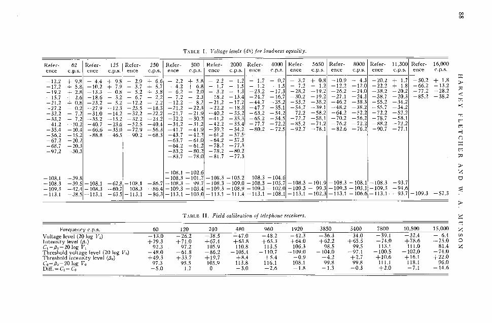
The experimental data for determining the relation between Lk and fk are given in Table I in terms of voltage levels. (Voltage level = 20 log l', where [' is the ean.f. across the receivers in
volts.) The pairs of values in each double column give the voltage levels of the reference tone and the pure tone having the frequency indicated at the top of the column when the two tones coming from the head receivers were judged to be equally loud when using the technique described in Appendix A. For example, in the second column it will be seen that for the 125-cycle tone when the voltage is +9.8 db above 1 volt then the voltage level for the reference tone must be 4.4 db below 1 volt for equality of loudness. The bottom set of numbers in each column gives the threshold values for this group of observers.
Each voltage level in Table I is the median of 297 observations representing the combined results of eleven observers. The method of
obtaining these is explained in Appendix A also. The standard deviation was computed and it was found to he somewhat larger for tests in which the tone differed most in frequency from the reference tone. The probable error of the com- bined result as computed in the usual way was between 1 and 2 db. Since deviations of any one observer's results from his own average are less than the deviations of his average from the average of the group, it would be necessary to increase the size of the group if values more representative of the average normal ear were desired.
The data shown in Table I can be reduced to the number of decibels above threshold if we
accept the values of this crew as the reference threshold values. However, we have already adopted a value for the 1000-cycle reference zero. As will be shown, our crew obtained a threshold for the reference tone which is 3 db above the reference level chosen.
It is not only more convenient but also more reliable to relate the data to a calibration of the
receivers in terms of physical measurements of the sound intensity rather than to the threshold values. Except in experimental work where the intensity of the sound can be definitely con-
trolled, it is obviously impractical to measure directly the threshold level by using a large group of obser•-ers having normal hearing. For most purposes it is •nore convenient to measure the intensity levels fi•, t•, .-- •, etc., directly rather than have them related in any way to the threshold of hearing.
In order to reduce the data in Table I to those
which one would obtain if the observers were
listening to a free wave and facing the source, we must obtain a field calibration of the telephone receivers used in the loudness comparisons. The calibration for the reference tone frequency has been explained previously and the equation
/• =/•+ 10 log (W,/gh) (5)
derived for the relation between the intensity of the reference tone and the electrical power in the receivers. The calibration consisted of
finding by means of loudness balances a power in the receivers which produces a tone equal in loudness to that of a free wave having an intensity level/•1.
For sounds other than the 1000-cycle reference tone a relation similar to Eq. (5) can be derived, namely,
•=01'-}-•0 log (W/W1),
where • and [[h are corresponding values found from loudness balances for each frequency or complex wave form of interest. If, as is usually assumed, a linear relation exists between • and 10 log W, then determinations of/• and I, V1 at one level are sufficient and it follows that a change in the power level of _X decibels will produce a corresponding change of ,• decibels in the intensity of the sound generated. Obviously the receivers must not be overloaded or this as-
sumption will not be valid. Rather than depend upon the existence of a linear relation between and 10 log 1V with no confirming data, the receivers used in this investigation were cali- brated at two widely separated levels.
Referring again to Table I, the data are expressed in terms of power levels. If, as receivers, the electrical constant, Eq. (11) can
voltage levels instead of was the case with our
impedance is essentially a be put in the form:
log (17 lr,) 02)
T^BLE I. Voltage levels (db) for loudness equality.
Refer- 62 Refer- 125 Refer- 250 Refer- 500 Refer- 2000 Refer- 4000 Refer- 5650 Refer- 8000 Refer- 11,300 Refer- 16,00• ence c.p.s. ence c.p.s. ence c.p.s. ence c.p.s. ence c.p.s. ence c.p.s. ence c.p.s. ence c.p.s. ence c.p.s. ence c.p.s.
--12.2 + 9.8 -- 4.4 + 9.8 -- 2.9 + 6.6 -- 2.2 + 5.8 -- 2.2 -- 1.2 -- 1.7 -- 0.7 -- 3.7 + 0.8 --10.9 -- 4.3 --20.2 + 1.7 --50.2 q- 1.: --17.2 + 5.8 --10.2 + 7.9 -- 3.7 + 5.7 -- 4.2 q- 6.8 -- 1.7 -- 1.5 -- 1.2 -- 1.5 -- 7.2 -- 1.2 --12.2 --12.0 --22.2 + 1.8 --66.2 --13.: --19.2 + 2.8 --13.3 -- 0.8 -- 5.2 + 5.8 -- 6.2 -- 2.0 -- 3.2 -- 1.3 --23.2 --17.3 --28.2 --19.2 --26.2 --24.0 --38.2 --20.2 --77.2 --28.: --15.7 + 2.6 --18.6 -- 3.2 -- 6.7 -- 2.2 -- 7.2 -- 2.3 --18.2 --13.4 --24.7 --16.7 --30.2 --19.2 --27.1 --24.3 --38.7 --20.3 --85.2 --38.: --21.2 + 0.8 --23.2 -- 5.2 --12.2 -- 2.2 --12.2 -- 8.2 --21.2 --17.2 --44.7 --35.2 --53.2 --38.2 --46.2 --38.3 --55.2 --34.2 --27.2 -- 0.2 --27.9 --12.3 --25.5 --18.3 --21.2 --22.3 --22.2 --18.3 --47.7 --35.1 --54.7 --39.1 --48.2 --38.2 --55.7 --34.2 --32.2 -- 7.2 --31.0 --14.2 --32.2 --22.2 --21.7 --21.9 --40.2 --35.2 --63.2 --54.2 --72.2 --58.2 --64.2 --52.2 --72.2 --52.2 --33.2 -- 7.2 --35.2 --15.2 --32.2 --23.2 --32.2 --30.2 --41.2 --35.3 --65.2 --54.5 --72.7 --58.1 --70.2 --56.2 --78.7 --58.1 --41.2 --10.2 --40.7 --23.6 --52.5 --40.4 --34.2 --31.2 --42.2 --35.4• --77.7 --72.2 --85.2 --71.2 --76.2 --72.2 --88.2 --72.2 --35.4 --10.4 --66.6 --35.0 --72.9 --56.3 --41.7 --41.9 --59.2 --54.2 --80.2 --72.5 --92.7 --78.1 --82.6 --76.2 --90.7 --77.1 --56.2 --15.2 --88.8 --46.5 --90.2 --68.3 --43.7 --42.2 --61.2 --57.5' --67.2 --20.2 --63.7 --61.0 --64.2 --57.3 --68.7 --20.3 --64.2 --61.2 --78.2 --77.3 --97.2 --30.3 --83.2 --80.2 --78.2 --80.2
--83.7 --78.0 --81.7 --77.3
-- 108.1 -- 102.6 --108.1 --39.8 --108.3 --101.7 --108.3 --105.2 --108.3 --104.6 --108.3 --39.5 --108.1 --62.8 --108.1 --86.7 --108.3- 99.7 --108.3--109.0 --108.3--105.7 --108.3--101.9 --108.3--108.1!--108.3 --93.7 --109.3 --42.4 --108.3 --60.7 --108.3 --86.4 --109.3 -- 103.4 -- 109.3 --108.9 -- 109.3 --102.0 --109.3 -- 99.3 --109.3 --103.1 --109.3 --94.6 --113.1 --38.5 --113.1 --63.5 --113.1 --86.3 --113.1 --103.(1 --113.1 --111.4 --113.1 --108.1 --113.1 --102.3 --113.1 --106.• --113.1 --93.7 --109.3 --57.:
>
TABLE II. Field calibration of telephone receivers.
Frequency c.p.s. 60 120 240 480 960 1920 3850 5400 7800 10,500 15,000 Voltage level (20 log V0 -- 13.0 --26.2 Intensity level (•t) +79.3 +71.0 C• =•- 20 log V• 92.3 97.2 Threshold voltage level (20 log Vo) -48.0 --61.8 Threshold intensity level (•5o) +49.3 +33.7 Co=t•o- 20 log Vo 97.3 95.5 Diff. = C•- Co -5.0 1.7
--38.5 --47.0 --48.2 --42.3 --36.3 --34.0 --39.1 --32.4 -- 6.4 +67.4 +63.8 +65.3 +64.0 +62.2 +65.5 +74.0 +78.6 +75.0 105.9 110.8 113.5 106.3 98.5 99.5 113.1 111.0 81.4
-- 86.2 -- 105.4 -- 110.7 -- 109.0 -- 104.0 --97.1 -- 100.5 --102.0 -- 74.0 +19.7 +8.4 +5.4 --0.9 --4.2 +2.7 +10.6 +16.1 +22.0 105.9 113.8 116.1 108.1 99.8 99.8 Ilia 118.1 96.0 0 --3.0 --2.6 --1.8 --1.3 --0.3 +2.0 --7.1 --14.6
LOUDNESS, ITS DEFINITION, MEASUREMENT AND CALCULATION 89
or
tl=20 log V+C, (13)
where V is the voltage across the receivers and C is a constant of the receivers to be determined
from a calibration giving corresponding values of th and 20 log V•. The calibration will now be described.
By using the sound stage and the technique of measuring field pressures described by Sivian and White • and by using the technique for making loudness measurements described in Appendix A, the following measurements were made. An electrical voltage V• was placed across the two head receivers such that the loudness
level produced was the same at each frequency. The observer listened to the tone in these head
receivers and then after 1« seconds silence listened to the tone from the loud speaker producing a free wave of the same frequency. The voltage level across the loud speaker neces- sary to produce a tone equally loud to the tone from the head receivers was obtained using the procedure described in Appendix A. The free wave intensity level fi• corresponding to this voltage level was measured in the manner de- scribed in Sivian and White's paper. Threshold values both for the head receivers and the loud
speaker were also observed. In these tests eleven observers were used. The results obtained are
given in Table II. In the second rmv values of 20 log V•, the voltage level, are given. The intensity levels, fi•, of the free wave which sounded equally loud are given in the third row. In the fourth row the values of the constant C, the calibration we are seeking, are given. The voltage level added to this constant gives the equivalent free wave intensity level. In the fifth, sixth and seventh rows, similar values are given which were determined at the threshold level. In the
bottom row the differences in the constants
determined at the two levels are given. The fact that the difference is no larger than the probable error is very significant. It means that through- out this wide range there is a linear relationship between the equivalent field intensity levels, •, and the voltage levels, 20 log V, so that the formula (13)
• L. J. Sivian and S. D. White, Minimum Audible Sound Fields, J. Acous. Soc. Am. 4, 288 (1933).
fi = 20 log 1'+ C
can be applied to our receivers with considerable confidence.
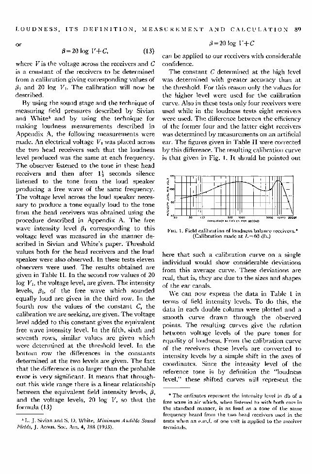
The constant C determined at the high level was determined with greater accuracy than at the threshold. For this reason only the values for the higher level were used for the calibration curve. Also in these tests only four receivers were used while in the loudness tests eight receivers were used. The difference between the efficiency of the former four and the latter eight receivers was determined by measurements on an artificial ear. The figures given in Table II were corrected by this difference. The resulting calibration curve is that given in Fig. 1. It should be pointed out
FIG. 1. Field calibration of loudness balance receivers.* (Calibration made at L=60 db.)
here that such a calibration curve on a single individual would show considerable deviations
from this aw.•rage curve. These deviations are real, that is, they are due to the sizes and shapes of the ear canals.
We can now express the data in Table I in terms of field intensity levels. To do this, the data in each double column were plotted and a smooth curve drawn through the observed points. The resulting curves give the relation between voltage levels of the pure tones for equality of loudness. From the calibration curve of the receivers these levels are converted to
intensity levels by a simple shift in the axes of coordinates. Since the intensity level of the reference tone is by definition the "loudness level," these shifted curves will represent the
* The ordinates represent the intensity level in db of a free wave in air which, when listened to with both ears in the standard manner, is as loud as a tone of the same frequency heard from the two head receivers used in the tests when an e.m.f. of one volt is applied to the receiver ternfinals.
90 HARVEY FLETCHER AND W. A. MUNSON
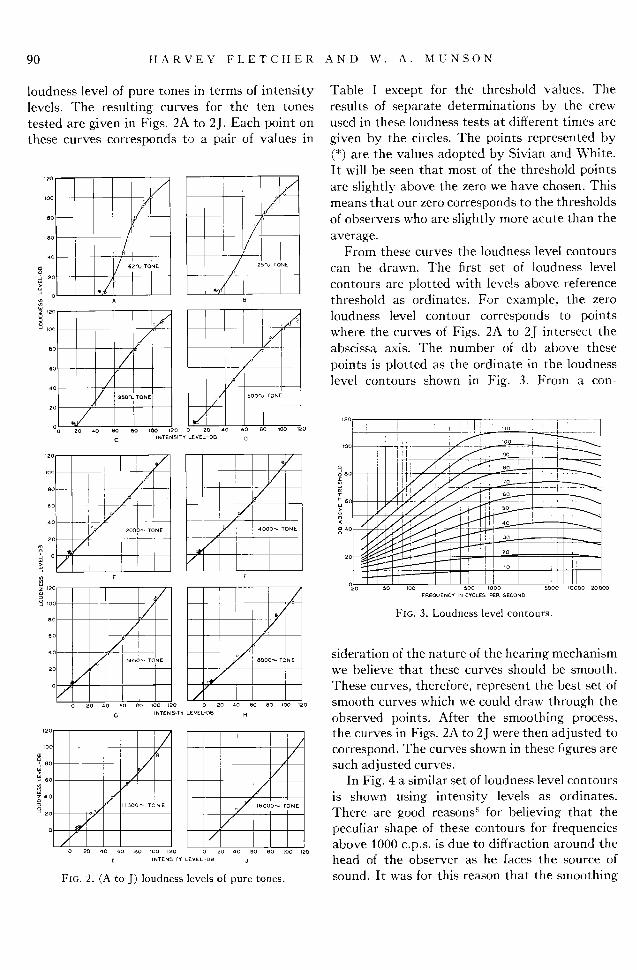
loudness level of pure tones in terms of intensity levels. The resulting curves for the ten tones tested are given in Figs. 2A to 2J. Each point on these curves corresponds to a pair of values in
40
o 100 120 0 20 40 60 80 •00 120
iNTENSiTY LEVEL-DB O
4C i , 4ooo• TONE
o 2o 40 6o 6o Ioo •2o o 2o 40 60 •o 1oo 12o
O INTœN•TY LEVEL-DB H
11300 TJNE
0 20 40 60 80 Ioo 120 0 20 40 60 80 too 120
! INTEN$4TY LEVEL-DB j
FIG. 2. (A to J) loudness levels of pure tones.
Table I except for the threshold values. The results of separate determinations by the crew used in these loudness tests at different times are
given by the circles. The points represented by (*) are the values adopted by Sivian and White. It will be seen that most of the threshold points are slightly above the zero we have chosen. This means that our zero corresponds to the thresholds of observers who are slightly more acute than the average.
From these curves the loudness level contours can be drawn. The first set of loudness level
contours are plotted with levels above reference threshold as ordinates. For example, the zero loudness level contour corresponds to points where the curves of Figs. 2A to 2J intersect the abscissa axis. The number of db above these
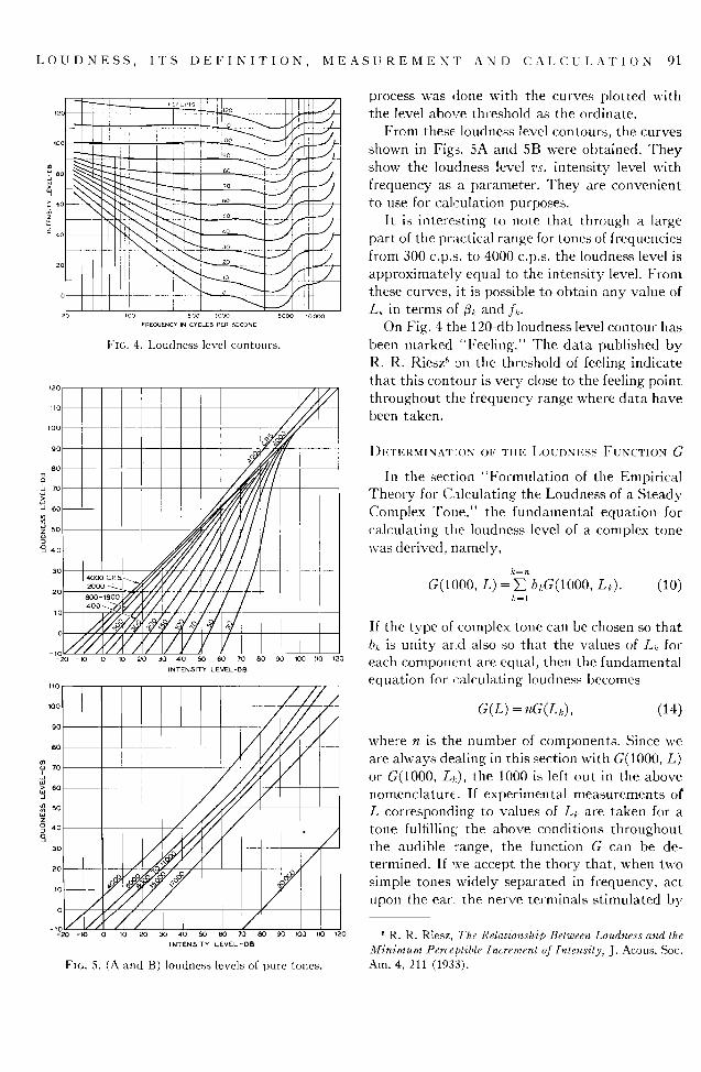
points is plotted as the ordinate in the loudness level contours shown in Fig. 3. From a con-
FIG. 3. Loudness level contours.
sideration of the nature of the hearing mechanism we believe that these curves should be smooth.
These curves, therefore, represent the best set of smooth curves which we could draw through the observed points. After the smoothing process, the curves in Figs. 2A to 2J xvere then adjusted to correspond. The curves shown in these figures are such adjusted curves.
In Fig. 4 a similar set of loudness level contours is shown using intensity levels as ordinates. There are good reasons s for believing that the peculiar shape of these contours for frequencies above 1000 c.p.s. is due to diffraction around the head of the observer as he faces the source of
sound. It was for this reason that the smoothing
LOUDNESS, ITS DEFINITION, MEASUREMENT AND CALCULATION 91
Fro. 4. Loudness level contours.
120
ioo
• •o
o
-I-020 -•O 0 10 •O 30 40 50 •0 70 •0 90 100 110 120
INTENSITY LEVœL-D8
FIG. 5. (A and B) loudness levels of pure tones.
process was done with the curves plotted with the level above threshold as the ordinate.
From these: loudness level contours, the curves shown in Figs. 5A and 5B were obtained. They show the loudness level rs. intensity level with frequency as a parameter. They are convenient to use for calculation purposes.
It is interesting to note that through a large part of the practical range for tones of frequencies froIn 300 c.p.s. to 4000 c.p.s. the loudness level is approximately equal to the intensity level. From these curves, it is possible to obtain any value of L• in terms of •a and f•.:.
On Fig. 4 the 120-db loudness level contour has been marked "Feeling." The data published by R. R. Riesz • on the threshold of feeling indicate that this contour is very close to the feeling point throughout the frequency range where data have been taken.
DETERMINATION OF TIlE LOUDNESS FUNCTION G
In the section "Formulation of the Empirical Theory for Calculating the Loudness of a Steady Complex Tone," the fundamental equation for calculating the loudness level of a complex tone was derived, namely,
G(1000, L) = Z b,:G(1000, Zt:). (10) k=l
tf the type of complex tone can be chosen so that b•. is unity and also so that the values of L• for each compommt are equal, then the fundamental equation for calculating loudness becomes
G(L) = nG(L•), (14)
where n is the number of components. Since we are always dealing in this section with G(1000, L) or G(1000, L;:), the 1000 is left out in the above nomenclature.. If experimental measurements ot' L corresponding to values of Lt. are taken for a tone fulfilling the above conditions throughout the audible :range, the function G can be de- termined. If we accept the thory that, when two simple tones widely separated in frequency, act upon the ear: the nerve terminals stimulated by
• R. R. Riesz, The Relationship Between Loudness and the Minimum Perceptible Increment of Intensity, J. Acous. Soc. Am. 4, 211 (1933).
92 HARVEY FLETCHER AND W. A. MUNSON
AND o-looo 2000
o 20 40 60 80 lOO 12o 14o LOUDNESS LEVEL OF EACH COMPONENT-OB
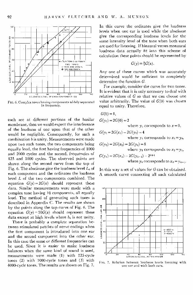
Fro. 6. Complex tones bavlng components widely separated in frequency.
each are at different portions of the basilar membrane, then we would expect the interference of the loudness of one upon that of the other would be negligible. Consequently, for such a combination b is unity. Measurements were made upon two such tones, the two components being equally loud, the first having frequencies of 1000 and 2000 cycles and the second, frequencies of 125 and 1000 cycles. The observed points are shown along the second curve from the top of Fig. 6. The abscissae give the loudness level Lk of each component and the ordinates the loudness level L of the two components combined. The equation G(y)=2G(x) should represent these data. Similar measurements were made with a
complex tone having 10 components, all equally loud. The method of generating such tones is described in Appendix C. The results are shown by the points along the top curve of Fig. 6. The equation G(y)=lOG(x) should represent these data except at high levels where bk is not unity.
There is probably a complete separation be- tween stimulated patches of nerve endings when the first component is introduced into one ear and the second component into the other ear. In this case the same or different frequencies can be used. Since it is easier to make loudness
balances when the same kind of sound is used, measurements were made (1) with 125-cycle tones (2) with 1000-cycle tones and (3) with 4000-cycle tones. The results are shown on Fig. 7.
In this curve the ordinates give the loudness levels when one ear is used while the abscissae
give the corresponding loudness levels for the same intensity level of the tone when both ears are used for listening. If binaural verses monaural loudness data actually fit into this scheme of calculation these points should be represented by
G(y) = «S(x).
Any one of these curves which was accurately determined would be sufficient to completely determine the function G.
For example, consider the curve for two tones. It is evident that it is only necessary to deal with relative values of G so that we can choose one
value arbitrarily. The value of G(0) was chosen equal to unity. Therefore,
G(0) = 1,
G(yo) = 2G(O) = 2 where y0 corresponds to x = 0,
G(y• = 2G(x•) = 2a(yo) = 4 where yl corresponds to x• =y0,
G(y•.) = 2G(x2) = 2G(y•) = 8 where y2 corresponds to x•=y•,
G(yk) = 2G(x•) = 2G(yk_•) = 2 where y• corresponds to x• = y•_•.
In this way a set of values for G can be obtained. A smooth curve connecting all such calculated
/
moo
• •o õ
20
0 20 40 60 •0 100 120 140
LOUDNESS LEVEL, BOTH EARS-DB
FIG. 7. Relation between loudness levels listening with one ear and with both ears.
LOUDNESS, ITS DEFINITION, MEASUREMEN'[' AND CALCULATION 93
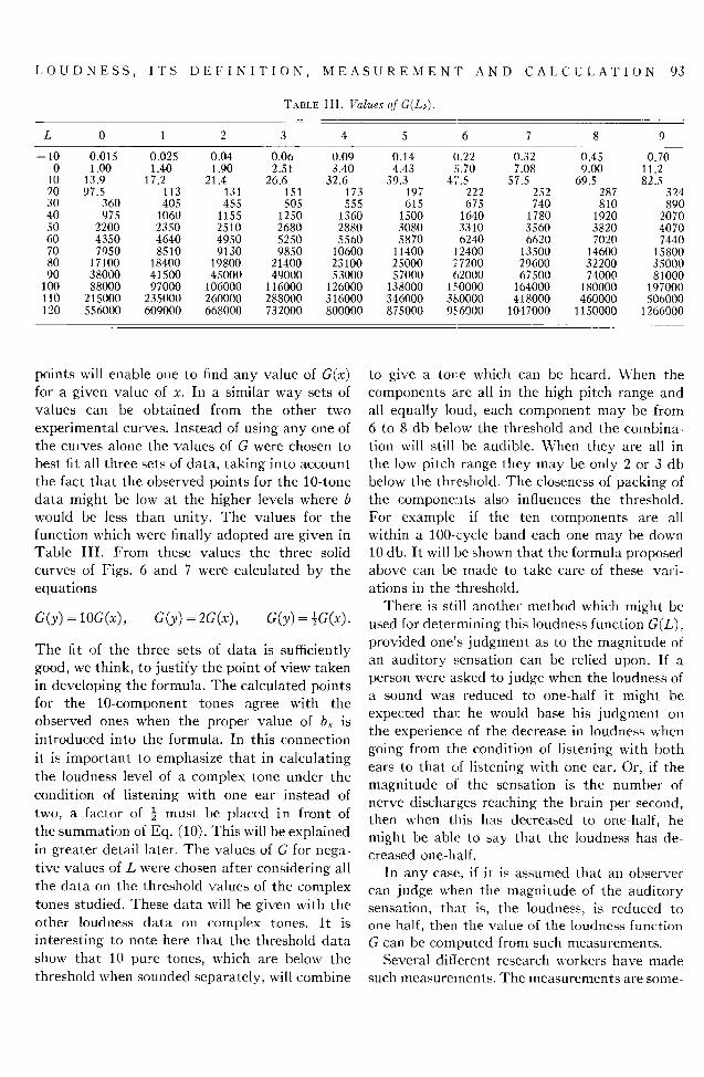
TABLE III. Values of G(L•).
L 0 1 2 3 4 5 6 7 8 9
-- 10 0.015 0.025 0.04 0.06 0.09 0.14 (I.22 0.32 0.45 0.70 0 1.00 1.40 1.90 2.51 3.40 4.43 5.70 7.08 9.00 11.2
10 13.9 17.2 21.4 26.6 32.6 39.3 4;'.5 57.5 69.5 82.5 20 97.5 113 131 151 173 197 222 252 287 324 30 360 405 455 505 555 615 675 740 810 890 40 975 1060 1155 1250 1360 1500 1640 1780 1920 2070 50 2200 2350 2510 2680 2880 3080 3310 3560 3820 4070 60 4350 4640 4950 5250 5560 5870 6240 6620 7020 7440 70 7950 8510 9130 9850 10600 11400 12400 13500 14600 15800 80 17100 18400 19800 21400 23100 25000 27200 29600 32200 35000 90 38000 41500 45000 49000 53000 57000 62000 67500 74000 81000
100 88000 97000 106000 116000 126000 138000 150000 164000 180000 197000 110 215000 235000 260000 288000 316000 346000 380000 418000 460000 506000 120 556000 609000 668000 732000 800000 875000 956000 1047000 1150000 1266000
points will enable one to find any value of G(x) for a given value of x. In a similar way sets of values can be obtained from the other two
experimental curves. Instead of using any one of the curves alone the values of G were chosen to
best fit all three sets of data, taking into account the fact that the observed points for the 10-tone data might be low at the higher levels where b would be less than unity. The values for the function which were finally adopted are given in Table III. From these values the three solid
curves of Figs. 6 and 7 were calculated by the equations
S(y) = 10G(x), G(y): 2G(x), S(y) = -}G(x).
The fit of the three sets of data is sufficiently good, we think, to justify the point of view taken in developing the formula. The calculated points for the 10-component tones agree with the observed ones when the proper value of b•, is introduced into the formula. In this connection
it is important to emphasize that in calculating the loudness level of a complex tone under the condition of listening with one ear instead of two, a factor of 21 must be placed in front of the summation of Eq. (10). This will be explained in greater detail later. The values of G for nega- tive values of L were chosen after considering all the data on the threshold values of the complex tones studied. These data will be given with the other loudness data on complex tones. It is interesting to note here that the threshold data show that 10 pure tones, which are below the threshold when sounded separately, will combine
to give a to•e which can be heard. When the components are all in the high pitch range and all equally loud, each component may be from 6 to 8 db below the threshold and the cmnbina-
tion will still be audible. When they are all in the low pitch range they may be only 2 or 3 db below the threshold. The closeness of packing of the components also influences the threshold. For example, if the ten components are all within a 100-cycle band each one may be down 10 db. It will be shown that the formula proposed above can be made to take care of these vari- ations in the 'threshold.
There is still another method which might be used for determining this loudness function G(L), provided one's judgment as to the magnitude of an auditory sensation can be relied upon. If a person were asked to judge when the loudness of a sound was reduced to one-half it might be expected that he would base his judgment on the experience of the decrease in loudness when going from the condition of listening with both ears to that of listening with one ear. Or, if the magnitude of the sensation is the number of nerve discharges reaching the brain per second, then when this has decreased to one-half, he might be able to say that the loudness has de- creased one-half.
In any case, if it is assumed that an observer can judge when the magnitude of the auditory sensation, that is, the loudness, is reduced to one-half, then the value of the loudness function G can be computed from such measurements.
Several different research workers have made
such measurements. The measurements are some-
94 HARVEY FLETCHER AND W. A. MUNSON
what in conflict at the present time so that they did not in any way influence the choice of the loudness function. Rather we used the loudness
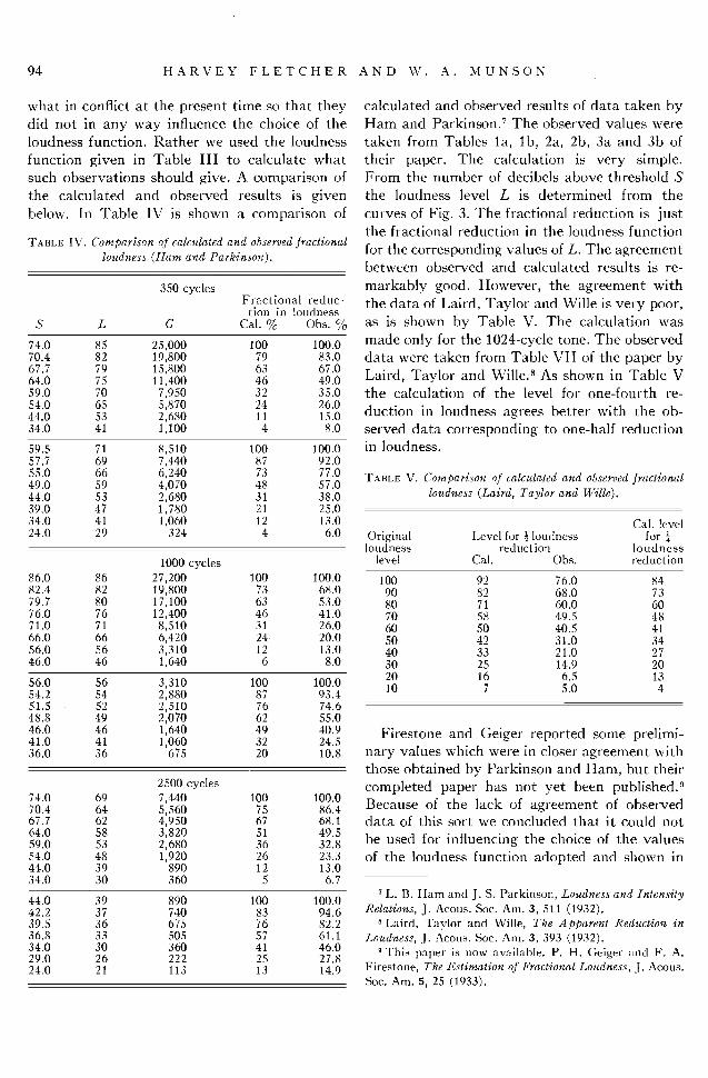
function given in Table III to calculate what such observations should give. A comparison of the calculated and observed results is given below. In Table IV is shown a comparison of
T^nLE IV. Comparison of calculated and observed fractional loudness (Ham and Parkinson).
350 cycles Fractional reduc-
tion in loudness
S L G Cal. % Obs. %
74.0 85 25,000 100 100.0 70.4 82 19,800 79 83.0 67.7 79 15,800 63 67.0 64.0 75 11,400 46 49.0 59.0 70 7,950 32 35.0 54.0 65 5,870 24 26.0 44.0 53 2,680 11 15.0 34.0 41 1,100 4 8.0
59.5 71 8,510 100 I00.0 57.7 69 7,440 87 92.0 55.0 66 6,240 73 77.0 49.0 59 4,070 48 57.0 44.0 53 2,680 31 38.0 39.0 47 1,780 21 25.0 34.0 41 1,060 12 13.0 24.0 29 324 4 6.0
1000 cycles 86.0 86 27,200 100 i00.0 82.4 82 19,800 73 68.0 79.7 80 17,100 63 53.0 76.0 76 12,400 46 41.0 71.0 71 8,510 31 26.0 66.0 66 6,420 24 20.0 56.0 56 3,310 12 13.0 46.0 46 1,640 6 8.0
56.0 56 3,310 100 100.0 54.2 54 2,880 87 93.4 51.5 52 2,510 76 74.6 48.8 49 2,070 62 55.0 46.0 46 1,640 49 40.9 41.0 41 1,060 32 24.5 36.0 36 675 20 10.8
2500 cycles 74.0 69 7,440 i00 70.4 64 5,560 75 67.7 62 4,950 67 64.0 58 3,820 51 59.0 53 2,680 36 54.0 48 1,920 26 44.0 39 890 12 34.0 30 360 5
calculated and observed results of data taken by Ham and Parkinson. 7 The observed values were
taken from Tables la, lb, 2a, 2b, 3a and 3b of their paper. The calculation is very simple. From the number of decibels above threshold S
the loudness level L is determined from the
curves of Fig. 3. The fractional reduction is just the fractional reduction in the loudness function
for the corresponding values of L. The agreement between observed and calculated results is re-
markably good. However, the agreement with the data of Laird, Taylor and Wille is very poor, as is shown by Table V. The calculation was made only for the 1024-cycle tone. The observed data were taken from Table VII of the paper by Laird, Taylor and Wille. a As shown in Table V the calculation of the level for one-fourth re-
duction in loudness agrees better with the ob- served data corresponding to one-half reduction in loudness.
T^BLE V. Comparison of calculated and observed fractional loudness (Laird, Taylor and Wille).
Cal. level
Original Level for « loudness for ¬ loudness reduction loudness
level Cal. Obs. reduction
100 92 76.O 84 90 82 68.0 73 80 71 60.0 60 7O 58 49.5 48 60 50 40.5 41 50 42 31.0 34 40 33 21.0 27 30 25 14.9 20 20 16 6.5 13 10 7 5.0 4
Firestone and Geiger reported some prelimi~ nary values which were in closer agreement with those obtained by Parkinson and Ham, but their completed paper has not yet been published. ø
100.0 Because of the lack of agreement of observed 86.4 68.1 data of this sort we concluded that it could not
49.5 be used for influencing the choice of the values 32.8
23.3 of the loudness function adopted and shown in 13.0
6.7
44.0 39 890 100 100.0 42.2 37 740 83 94.6 39.5 36 675 76 82.2 36.8 33 505 57 61.1 34.0 30 360 41 46.0 29.0 26 222 25 27.8 24.0 21 113 13 14.9
7 L. B. Ham and J. S. Parkinson, Loudness and Intensity Relations, J. Acous. Soc. Am. 3, 511 (1932).
• Laird, Taylor and Wille, The Apparent Reduction in Loudness, J. Acous. Soc. Am. 3, 393 (1932).
9 This paper is now available. P. H. Geiger and F. A. Firestone, The Estimation of Fractional Loudness, J. Acous. Soc. Am. 5, 25 (1933).
LOUDNESS, ITS DEFINITION, MEASUREMEN'[' AND CAI. CUI•ATION 95
Table III. It is to be hoped that more data of this type will be taken until there is a better agreement between observed results of different observers. It should be emphasized here that changes of the level above threshold correspond- ing to any fixed increase or decrease in loudness will, according to the theory outlined in this paper, depend upon the frequency of the tone when using pure tones, or upon its structure when using complex tones.
DETERMINATION OF THE FORMULA FOR
CALCULATING bk
Having now determined the function G for all values of L or Lk we can proceed to find methods of calculating b•. Its value is evidently dependent upon the frequency and intensity of all the other components present as well as upon the com- ponent being considered. For practical computa- tions, simplifying assumptions can be .made. In most cases the reduction of b• from unity is principally due to the adjacent component on the side of the lower pitch. This is due to the fact that a tone masks another tone of higher pitch very .much more than one of lower pitch. For example, in most cases a tone which is 100 cycles higher than the masking tone would be masked when it is reduced 25 db below the level
of the masking tone, whereas a tone 100 cycles lower in frequency will be masked only when it is reduced from 40 to 60 db below the level of
the masking tone. It will therefore be assumed that the neighboring component on the side of lower pitch which causes the greatest masking will account for all the reduction in bk. Desig- nating thi's component with the subscript m, meaning the masking component, then we have bx. expressed as a function of the following variables.
bk = B(f•., f,,,, S•., S,•), (15)
where f is the frequency and S is the level above threshold. For the case when the level of the kth
component is T db below the level of the masking component, where T is just sufficient for the component to be masked, then the value of b would be equal to zero. Also• it is reasonable to assume that when the masking component is at a level somewhat less than T db below the kth
component, the latter will have a value of b•
which is unity. It is thus seen that the funda- mental of a series of tones will always have a value of b• equal to unity.
For the case when the masking component and the kth component have the same loudness, the function representing b• will be considerably simplified, particularly if it were also found to be independent of f• and only dependent upon the differenos between fk and j;,•. From the theory of hearing one xvould expect that this would be approximately true for the following reasons:
The distance in millimeters between the po- sitions of maximum response on the basilar membrane for the two components is more nearly proportional to differences in pitch than to differences in frequency. However, the peaks are sharpest in the high frequency regions where the distances on the basilar membrane for a
given/xf are smallest. Also, in the low frequency region where the distances for a given /xf are largest, these. peaks are broadest. These two factors tend to make the interference between
two components having a fixed difference in frequency approximately the same regardless of their position on the frequency scale. However, it would be extraordinary if these two factors
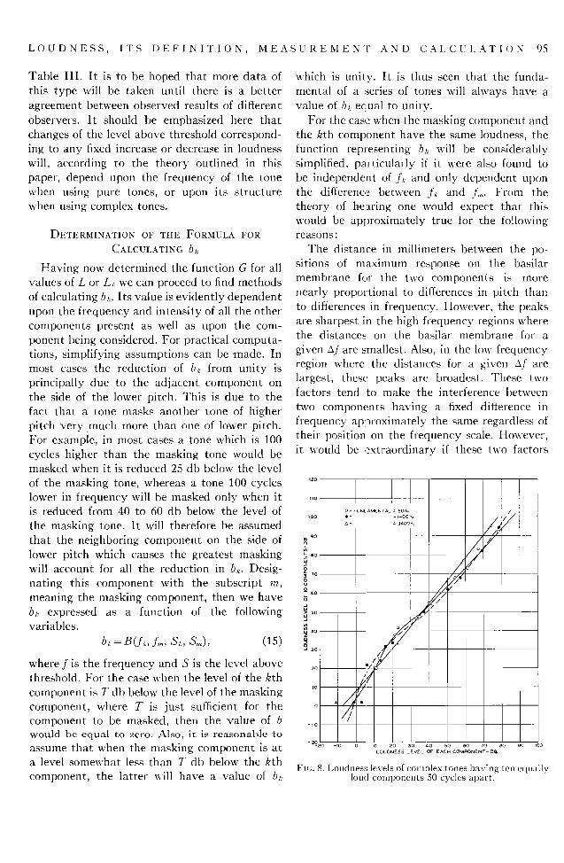
FIG. 8. Loudness levels of complex tones having ten equally loud components 50 cycles apart.
96 HARVEY FLETCHER AND W. A. MUNSON
just balanced. To test this point three complex tones having ten components with a common zXf of 50 cycles were tested for loudness. The first had frequencies of 50-100-150...500, the second 1400-1450... 1900, and the third 3400- 3450...3900. The results of these tests are
shown in Fig. 8. The abscissae give the loudness level of each component and the ordinates the measured loudness level of the combined tone.
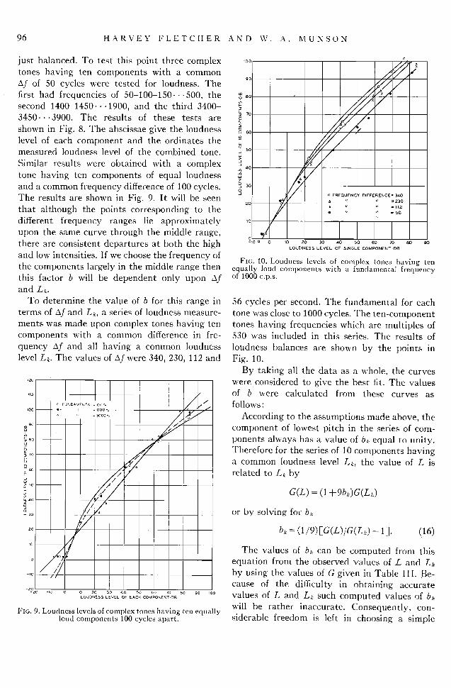
Similar results were obtained with a complex tone having ten components of equal loudness and a common frequency difference of 100 cycles. The results are shown in Fig. 9. It will be seen that although the points corresponding to the different frequency ranges lie approximately upon the same curve through the middle range, there are consistent departures at both the high and low intensities. If we choose the frequency of the components largely in the middle range then this factor b will be dependent only upon zXf and Lk.
To determine the value of b for this range in terms of 6f and Lk, a series of loudness measure- ments was made upon complex tones having ten components with a common difference in fre- quency zXf and all having a common loudness level L•. The values of zXf were 340, 230, 112 and
20 -10 0 10 20 30 40 50 60 70 80 90 100 L0U0NES$ LEVEL OF EACH COMPONENT-DB
FzG. 9. Loudness levels of complex tones having ten equally loud components 100 cycles apart.
u 60
o•
,.-d, so >
u, 40
J o FREQUENCY DIFFERENCE- 340
/
0_, ø o"P x
FIG. 10. Loudness levels of complex tones having ten equally loud components with a fundamental frequency of 1000 c.p.s.
56 cycles per second. The fundamental for each tone was close to 1000 cycles. The ten-component tones having frequencies which are multiples of 530 was included in this series. The results of
loudness balances are shown by the points in Fig. 10.
By taking all the data as a whole, the curves were considered to give the best fit. The values of b were calculated from these curves as follows:
According to the assumptions made above, the component of lowest pitch in the series of com- ponents always has a value of b•. equal to unity. Therefore for the series of 10 components having a common loudness level L•, the value of L is related to Lk by
G(L) = (1 +9b•)G(LD
or by solving for b•.,
b• = (1/9)[-G(L)/G(Lk) - 1]. (16)
The values of b•. can be computed from this equation from the observed values of L and L• by using the values of G given in Table III. Be- cause of the difficulty in obtaining accurate values of L and L• such computed values of bk will be rather inaccurate. Consequently, con- siderable freedom is left in choosing a simple
LOUDNESS, ITS DEFINITION, MEASUREMENT AND CALCULATION 97
5.0
3.0
4.0
X 2.0
1.0
0 0 20 40 60 80 100 120
LOUONE$1• LEVEL OF COMPONENT'OB
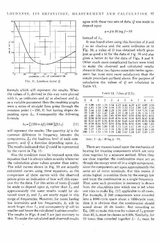
FIG. 11. Loudness factor Q.
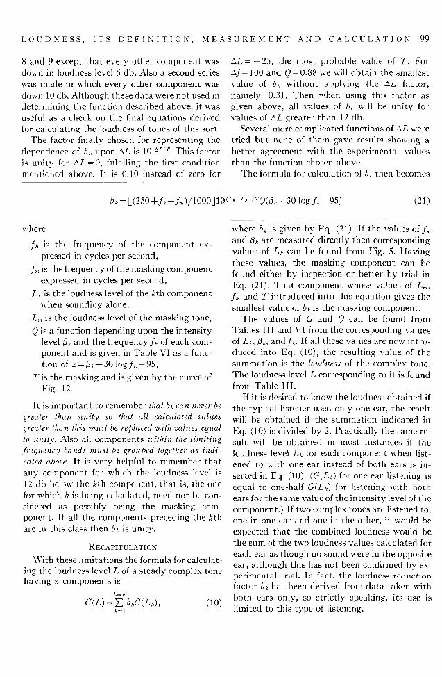
formula which will represent the results. When the values of b/, derived in this way were plotted with bk as ordinates and zXf as abscissae and Lk as a variable parameter then the resulting graphs were a series of straight lines going through the common point (-250, 0) but having slopes de- pending upon L•,. Consequently the following formula
bk = [-(250+/xf)/lOOO-]Q(L•.) (17)
will represent the results. The quantity Af is the common difference in frequency between the components, Lk the loudness level of each com- ponent, and Q a function depending upon Lk. The results indicated that Q could be represented by the curve in Fig. 11.
Also the condition must be imposed upon this equation that b is always taken as unity whenever the calculation gives values greater than unity. The solid curves shown in Fig. 10 are actually calculated curves using these equations, so the comparison of these curves with the observed points gives an indication of how well this equa- tion fits the data. For this series of tones Q could be made to depend upon fi• rather than L• and approximately the same results would be ob- tained since fi• and L• are nearly equal in this range of frequencies. However, for tones having low intensities and low frequencies, fik will be much larger than L7• and consequently Q will be smaller and hence the calculated loudness smaller.
The results in Figs. 8 and 9 are just contrary to this. To make the calculated and observed results
agree with these two sets of data, Q was made to depend upon
x=fi+30 log f-95
instead of L•.
It was found when using this function of/5 and f as an abscissa and the same ordinates as in Fig. 10, a value of Q was obtained which gives just as good a fit for the data of Fig. 10 and also gives a better fit for the data of Figs. 8 and 9. Other much more complicated factors were tried to make the observed and calculated results
shown in these two figures come into better agree- ment but none were more satisfactory than the simple procedure outlined above. For purpose of calculation the values of Q are tabulated in Table VI.
•I'^]•L• VI. Values of Q(X).
X 0 1 2 3 4 5 6 7 8 9
0 5.00 4.88 4.76 4.64 4.53 10 3.82 3.70 3.58 3.46 3.35 20 2.64 2.52 ;!.40 2.28 2.16 30 1.60 1.53 1.47 1.40 1.35 40 1.09 1.06 1.03 1.01 0.99 50 0.90 0.90 0.89 0.89 0.88 60 0.88 0.88 0.88 0.88 0.88 70 0.90 0.91 (}.92 0.93 0.94 80 1.04 1.06 1.08 1.10 1.13 90 1.27 1.29 1.31 1.34 1.36
100 1.51 1.53 1.55 1.58 1.60
4.41 4.20 4.17 4.05 3.94 3.33 3.11 2.99 2.87 2.76 2.05 1.95 1.85 1.76 1.68 1.30 1.25 1.20 1.16 1.13 0.97 0.95 0.94 0.92 0.91 0.88 0.88 0.88 0.88 0.88 0.88 0.88 0.89 0.89 0.90 0.96 0.97 0.99 1.00 1.02 1.15 1.17 1.19 1.22 1.24 1.39 1.41 1.44 1.46 1.48 1.62 1.64 1.67 1.69 1.71
Note: X=•t.+30 log fz.-95.
There are reasons based upon the mechanics of hearing for treating components which are very close together by a separate method. When they are close together the combination must act as though the energy were all in a single component, since the components act upon approximately the same set of nerve terminals. For this reason it
seems logical ro combine them by the energy law and treat the combination as a single frequency. That some such procedure is necessary is shown from the absurdities into which one is led when
one tries to make Eq. (17) applicable to all cases. For example, if 100 components were crowded into a 1000-cycle space about a 1000-cycle tone, then it is obvious that the combination should
sound about 20 db louder. But according to Eq. (10) to make this true for values of L• greater than 45, bk must be chosen as 0.036. Similarly, for 10 tones thus crowded together L-L• must be
98 HARVEY FLETCHER AND W. A. MUNSON
about 10 db. and therefore be=0.13 and then for two such tones L-L• must be 3 db and the cor-
responding value of b• = 0.26. These three values must belong to the same condition zXf= 10. It is evident then that the formulae for b given by Eq. (17) will lead to very erroneous results for such components.
In order to cover such cases it was necessary to group together all components within a certain frequency band and treat them as a single com- ponent. Since there was no definite criterion for determining accurately what these limiting bands should be, several were tried and ones selected which gave the best agreement between com- puted and observed results. The following band widths were finally chosen:
For frequencies below 2000 cycles, the band width is 100 cycles; for frequencies between 2000 and 4000 cycles, the band width is 200 cycles; for frequencies between 4000 and 8000 cycles, the band width is 400 cycles; and for frequencies be- tween 8000 and 16,000 cycles, the band width is 800 cycles. If there are k components within one of these limiting bands, the intensity I taken for the equivalent single frequency component is given by
I= E I• = • 10 •mø. (18)
A frequency must be assigned to the combination. It seems reasonable to assign a weighted value of f given by the equation
f=•. f•,Ie/I=Z f•10a•/lø,/E 10ateø. (19)
Only a small error will be introduced if the mid- frequency of such bands be taken as the fre- quency of an equivalent component except for the band of lowest frequency. Below 125 cycles it is important that the frequency and intensity of each component be known, since in this region the loudness level Le changes very rapidly with both changes in intensity and frequency. How- ever, if the intensity for this band is lower than that for other bands, it will contribute little to the total loudness so that only a small error will be introduced by a wrong choice of frequency for the band.
This then gives a method of calculating be when the adjacent components are equal in loud- ness. When they are not equal let us define the difference/XL by
z•L = L•--L•. (20)
Also let this difference be T when L• is adjusted so that the masking component just masks the component k. Then the function for calculating b must satisfy the following conditions:
b•=[-(250+z_Xf)/lOOO-]Q when ,XL=0,
b•=0 when•L=-T.
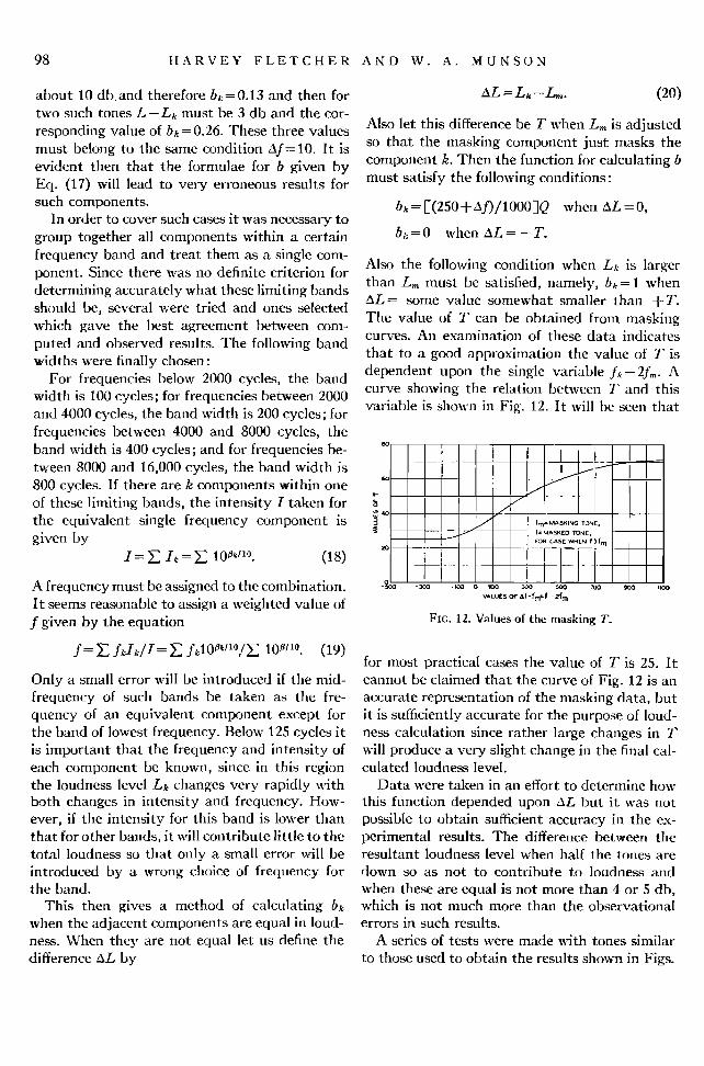
Also the following condition when L• is larger than L•, must be satisfied, namely, be= 1 when 6L= some value somewhat smaller than +T. The value of T can be obtained from masking curves. An examination of these data indicates
that to a good approximation the value of T is dependent upon the single variable f•.--2f,,. A curve showing the relation between T and this variable is shown in Fig. 12. It will be seen that
I I for CASE WHϥ f)fm
VALU•:S a•' af-fm-f -•fm
FIG. 12. Values of the masking T.
for most practical cases the value of T is 25. It cannot be claimed that the curve of Fig. 12 is an accurate representation of the masking data, but it is sufficiently accurate for the purpose of loud- ness calculation since rather large changes in T will produce a very slight change in the final cal- culated loudness level.
Data were taken in an effort to determine how
this function depended upon aXL but it was not possible to obtain sufficient accuracy in the ex- perimental results. The difference between the resultant loudness level when half the tones are
down so as not to contribute to loudness and
when these are equal is not more than 4 or 5 db, which is not much more than the observational errors in such results.
A series of tests were made with tones similar
to those used to obtain the results shown in Figs.
LOUDNESS, ITS DEFINITION, MEASUREMENT AND CALCULATION 99
8 and 9 except that every other component was down in loudness level 5 db. Also a second series
was made in which every other component was down 10 db. Although these data were not used in determining the function described above, it was useful as a check on the final equations derived for calculating the loudness of tones of this sort.
The factor finally chosen for representing the dependence of bk upon /XL is 10 aL/v. This factor is unity for AL=0, fulfilling the first condition mentioned above. It is 0.10 instead of zero for
zXL=-25, the most probable value of T. For /x f= 100 and Q = 0.88 we will obtain the smallest value of b/• without applying the 2•L factor, namely, 0.31. Then when using this factor as given above, all values of b•,: will be unity for values of AL greater than 12 db.
Several more complicated functions of zXL were tried but no•e of them gave results showing a better agreement with the experimental values than the function chosen above.
The formula for calculation of b•: then becomes
b• = [(250+f• -f,•)/lOOO•lO(•-•"')/rO(3•:+30 log f•- 95) (21)
where
f• is the frequency of the component ex- pressed in cycles per second,
f,,• is the frequency of the masking component expressed in cycles per second,
L•. is the loudness level of the kth component when sounding alone,
L• is the loudness level of the masking tone,
Q is a function depending upon the intensity level fi• and the frequency f•; of each ponent and is given in Table VI as a func- tion of x=fi•+30 logf•-95,
T is the masking and is given by the curve of Fig. 12.
It is important to remember that b• can never be greater than unity so that all calculated values greater than this mu.•t be replaced with values equal to unity. Also all components within the limiting frequency bands must be grouped together as indi- cated above. It is very helpful to remember that any component for which the loudness level is 12 db below the kth component, that is, the one for xvhich b is being calculated, need not be con- sidered as possibly being the masking com- ponent. If all the components preceding the kth are in this class then b• is unity.
RECAPITULATION
With these limitations the formula for calculat-
ing the loudness level L of a steady complex tone having n components is
G(L) = 5• b•G(L•), (10)
where b•. is given by Eq. (21). If the values off• and • are measured directly then corresponding values of L• can be found from Fig. 5. Having these values, the masking component can be found either by inspection or better by trial in Eq. (21). That component whose values of L,•, f,• and T introduced into this equation gives the smallest value of b• is the masking component.
The values of G and Q can be found from Tables III and VI from the corresponding values of L•-, ilk, and f•. If all these values are now intro- duced into Eq. (10), the resulting value of the summation is. the loudness of the complex tone. The loudness level L corresponding to it is found from Table I[I.
If it is desired to know the loudness obtained if
the typical listener used only one ear, the result will be obtained if the summation indicated in
Eq. (10) is divided by 2. Practically the same re- sult will be obtained in most instances if the
loudness level L• for each component when list- ened to ;vith one ear instead of both ears is in-
serted in Eq. (10). (G(Lx.) for one ear listening is equal to one--half G(L•) for listening with both ears for the same value of the intensity level of the component.) If two complex tones are listened to, one in one ear and one in the other, it would be expected that the combined loudness would be the sum of the two loudness values calculated for
each ear as though no sound were in the opposite ear, although this has not been confirmed by ex- perimental trial. In fact, the loudness reduction factor b• has been derived from data taken with
both ears only, so strictly speaking, its use is limited to this type of listening.
100 HARVEY FLETCHER AND W. A. MUNSON
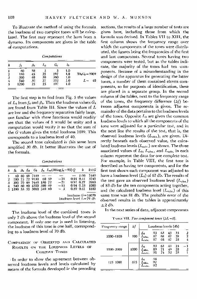
To illustrate the method of using the formula the loudness of two complex tones will be calcu- lated. The first may represent the hum from a dynamo. Its components are given in the table of computations.
Computations
1 60 50 3 3 1.0 2 180 45 25 191 1.0 ZbeGle= 1009 3 300 40 30 360 1.0 4 540 30 27 252 1.0 L = 40 5 1200 25 25 197 1.0
The first step is to find from Fig. 5 the values of L• from f, and •t•. Then the loudness values G, are found from Table III. Since the values of L are low' and the frequency separation fairly large, one familiar with these functions would readily see that the values of b would be unity and a computation would verify it so that the sum of the G values gives the total loudness 1009. This corresponds to a loudness level of 40.
The second tone calculated is this same hum
amplified 30 db. It better illustrates the use of the formula.
Computations
k f• • L• G• f,, L,•(301ogf•-95)Q b bXG 1 60 80 69 7440 -- -- 1.00 7440 2 180 75 72 9130 60 69 --28 0.91 0.41 3740 3 300 70 69 7440 180 72 --21 0.91 0.27 2010 4 540 60 60 4350 300 69 --13 0.94 0.23 1000 5 1200 55 55 3080 540 60 -- 3 0.89 0.61 1880
loudness G= 16070 loudness level L = 79 db
The loudness level of the combined tones is
only 7 db above the loudness level of the second component. If only one ear is used in listening, the loudness of this tone is one-half, correspond-
ing to a loudness level of 70 db.
COMPARISON OF OBSERVED AND CALCULATED RESULTS OXi THE LOUDNESS LEVELS OF
COl•IPLEX TONES
ß In order to show the agreement between ob- served loudness levels and levels calculated by means of the formula developed iv the preceding
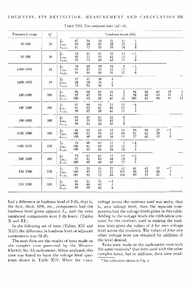
sections, the results of a large number of tests are given here, including those from which the formula was derived. In Tables VII to XIII, the first column shows the frequency range over which the components of the tones were distrib- uted, the figures being the frequencies of the first and last components. Several tones having two components were tested, but as the tables indi- cate, the majority of the tones had ten com- ponents. Because of a misunderstanding in the design of the apparatus for generating the latter tones, a number of them contained eleven com- ponents, so for purposes of identification, these are placed in a separate group. In the second column of the tables, next to the frequency range of the tones, the frequency difference (•f) be- tween adjacent components is given. The re- mainder of the data pertains to the loudness levels of the tones. Opposite L• are given the common loudness levels to which all the components of the tone were adjusted for a particular test, and in the next line the results of the test, that is, the observed loudness levels (Lo•,,.), are given. Di- rectly beneath each observed value, the calcu- lated loudness levels (L•.) are shown. The three associated values of L•, Loh,., and L•.•t½. in each column represent the data for one complete test. For example, in Table VIII, the first tone is described as having ten components, and for the first test shown each component was adjusted to have a loudness level (L•) of 67 db. The results of the test gave an observed loudness level (Lo•,.) of 83 db for the ten components acting together, and the calculated loudness level (L•.,lo.) of this same tone was 81 db. The probable error of the observed results in the tables is approximately 4-2 db.
In the next series of data, adjacent components
T•BLE VII. Two component tones (AL=0).
Frequency range
1000-1100
1000-2000
125-1000
000
875
Loudness levels (db)
L• 83 63 43 23 2 Lo•,•. 87 68 47 28 2 Leale. 87 68 47 28 4
Lt: 83 63 43 23 --1 Lon•. 89 71 4o 28 2 Le•c. 91 74 52 28 l
L& 84 Lobs. 92 ' Leale. 92
LOUDNESS, ITS DEFINITI()N, MEASUREMENT AND CALCULATION 101
TABLE VIII. Ten component tones (zXL=0).
Frequency range
50 500
50 500
1400 1895
1400-1895
100-1000
100 1000
100 1000
3100 3900
1100-3170
260-2600
530 5300
530 5300
Loudness levels (db)
Lk 67 54 33 21 11 -- 1 Lo•,•. 83 68 47 38 2:0 2 L•d•. 81 72 53 39 2:4 8
Lk 78 61 41 23 13 --1 Lobs. 92 73 53 42 2:5 2 L•ale. 91 77 60 42 27 8
L• 78 69 50 16 6 -1 Lobs. 94 82 62 32 22 2 L•::m•. 93 83 65 31 17 0
L• 57 37 20 3 Lobs. 68 50 34 2 Le=•. 73 52 36 5
L, 84 64 43 24 2 84 64 43 24 2 Lobs. 95 83 59 41 2 94 80 63 44 2 L•,=m,. 100 83 68 47 12 100 83 68 47 12
L• 81 64 43 23 13 -4 Lo•s. 93 82 65 49 33 2 Lcale. 98 83 68 45 27 3
L• 83 63 43 23 0 Lob•. 95 79 59 43 2 L•.•d•. 99 82 68 45 9
L• 83 63 43 23 78 59 48 27 - 7 Lo•,•. 100 82 59 32 99 81 62 38 2 Leal½. 100 80 60 38 95 77 65 42 0
L• 79 60 41 17 7 --4 Lobs. 100 81 65 33 22 2 L½•t0. 100 83 64 34 18 3
L• 79 62 42 23 13 - 2 Lobs. 97 82 65 44 28 2 Leale. 100 85 68 45 27 5
L• 75 53 43 25 82 61 43 17 -- 2 Lob•. 100 83 73 52 105 90 73 40 2 Lcale. 101 82 72 48 108 89 72 34 5
Lk 61 41 21 --3 Lobs. 89 69 45 2 Lea•½. 89 70 42 4
had a difference in loudness level of 5 db, that is, the first, third, fifth, etc., components had the loudness level given opposite L•, and the even numbered components were 5 db lower. (Tables X and XI.)
In the following set of tests (Tables XII and XIII) the difference in loudness level of adjacent components was 10 db.
The next data are the results of tests made on
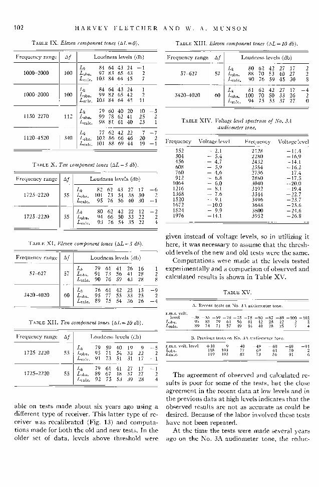
the complex tone generated by the Western Electric No. 3A audiometer. When analyzed, this tone was found to have the voltage level spec- trum shown in Table XIV. When the r.m.s.
voltage across the receivers used was unity, that is, zero voltage level, then the separate com- ponents had the voltage levels given in this table. Adding to the voltage levels the calibration con- stant for the receivers used in making the loud- ness tests giw•s the values of fi for zero voltage level across the receivers. The values of • for any other voltage level are obtained by addition of the level desired.
Tests were made on the audiometer tone with the same receivers* that were used with the other
complex tones, but in addition, data were avail-
* See calibration shown in Fig. 1.
102 HARVEY FLETCHER
TABLE IX. Eleven component tones (/•L=0).
Frequency range
1000-2000
1000-2000
1150-2270
1120-4520
100
100
112
340
Loudness levels (db)
L• 84 64 43 24 --1 Loba. 97 83 65 43 2 Lc•le. 103 84 64 45 7
Lk 84 64 43 24 1 Lobs. 99 82 65 42 2 Leale. 103 84 64 45 11
Lk 79 60 40 20 10 --5 Lobs. 99 78 62 41 25 2 Lc•ic. 98 81 61 40 23 1
Lk 77 62 42 22 7 Lobs. 102 86 66 46 20 Le•lc. 101 88 69 44 19
TABLE X. Ten component tones (•L = 5 db).
Frequency range
1725-2220
1725-2220
55
55
Loudnesslevels (db)
L• 82 62 43 27 17 --6 Loba. 101 73 54 38 30 2 Lcalc. 95 76 56 40 30 -1
L• 80 62 42 22 12 -2 Lobs. 94 66 50 33 22 2 Lc•t•. 93 76 54 35 22 4
TABLE XI. Eleven component tones (AL = 5 db).
Frequency range
57 627
3420-4020
57
60
Loudness levels (db)
L• 79 61 41 26 16 1 Lobs. 91 73 56 41 28 2 Lc,,lc. 90 76 59 43 28 8
L• 76 61 42 25 15 -9 Loba. 95 77 55 33 25 2 Lcfii. 89 75 54 36 26 --4
TABLE XII. Ten cmnponent tones (zXL= 10 db).
Frequency range
1725-2220
1725-2220
•f
55
55
Loudness levels (db)
L• 79 59 40 19 9 --5 Lobs. 95 7l 54 33 22 2 Leale. 91 73 51 31 17 --1
Lk 79 61 41 27 17 --1 Lob•. 89 67 48 37 27 2 LcMc. 92 75 53 39 28 4
able on tests made about six years ago using a different type of receiver. This latter type of re- ceiver was recalibrated (Fig. 13) and computa- tions made for both the old and new tests. In the
older set of data, levels above threshold were
AND W. A. MUNSON
TABLE XIII. Eleven component tones (•XL= 10 db).
Frequency range
57-627
3420-4020
af
57
60
Loudnesslevels (db)
L• 80 62 42 27 17 2 Lob•. 88 70 53 40 27 2 L•lc. 90 76 59 45 30 8
L• 81 62 42 27 17 --4 Lobs. 100 70 50 33 26 2 L•x•. 94 75 53 37 27 0
TABLE XIV. Voltage level spectrum of No. 3A audiometer tone.
--7 2
- 1 Frequency Voltage level Frequency Voltage level 152 -- 2.1 2128 --11.4 304 -- 5.4 2280 -- 16.9 456 -- 4.7 2432 --14.1 608 -- 5.9 2584 -- 16.2 760 -- 4.6 2736 -- 17.4 912 -- 6.8 2880 -17.5
1064 -- 6.0 3040 --20.0 1216 -- 8.1 3192 --19.4 1368 -- 7.6 3344 -- 22.7 1520 -- 9.1 3496 --23.7 1672 -- 10.0 3648 -- 25.6 1824 -- 9.9 3800 -- 24.6 1976 - 14.1 3952 --26.8
given instead of voltage levels, so in utilizing it here, it was necessary to assume that the thresh- old levels of the new and old tests were the same.
Computations were made at the levels tested experimentally and a comparison of observed and calculated results is shown in Table XV.
TABLE XV.
A. Recent tests on No. 3A audiometer tone.
r.m.s. volt. level --38 --55 --59 --70 --75 --78 --80 --87 --89 --100 --102
Lobs. 95 85 79 61 56 41 42 28 22 2 2 Leale. 89 74 71 57 49 44 40 :28 25 7 4
B. P•evious tests on No. 3A audiometer tone.
r.m.s. volt. level +10 9 --40 --49 --6(I --69 --91 Loba. 118 103 77 69 6l 50 2 LcMc. 119 103 82 73 56 41 6
The agreement of observed and calculated re- suits is poor for some of the tests, but the close agreement in the recent data at loxv levels and in the previous data at high levels indicates that the observed results are not as accurate as could be desired. Because of the labor involved these tests
have not been repeated. At the time the tests were made several years
ago on the No. 3A audiometer tone, the reduc-
LOUDNESS, ITS DEFINITION, MEASUREMENT AND CALCULATION 103
,:
FIG. 13. Calibration of receivers for tests on the No. 3A audiometer tone
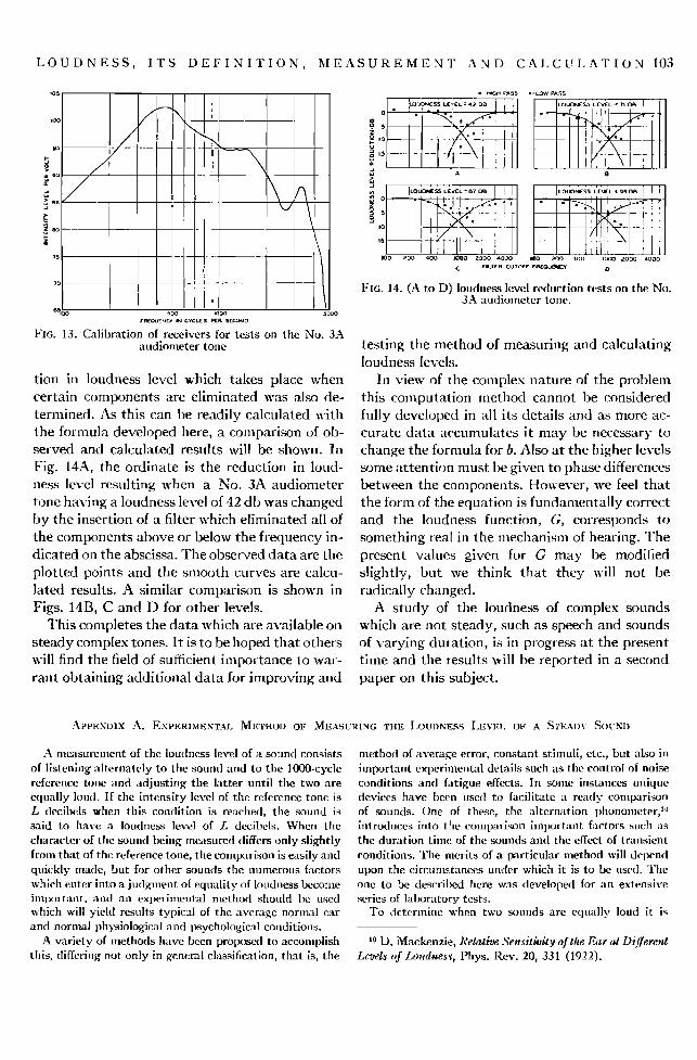
rio,1 in loudness level which takes place when certain components are eliminated was also de- ternfined. As this can be readily calculated with the formula developed here, a comparison of ob- served and calculated results will be shown. In
Fig. 14A, the ordinate is the reduction in loud- ness level resulting when a No. 3A audiometer tone having a loudness level of 42 db was changed by the insertion of a filter which eliminated all of the components above or below the frequency in- dicated on the abscissa. The observed data are the
plotted points and the smooth curves are calcu- lated results. A similar comparison is shown in Figs. 14B, C and D for other levels.
This completes the data which are available on steady complex tones. It is to be hoped that others will find the field of sufficient importance to war- rant obtaining additional data for improving and
FiG. 14. (A to D) Iouduess level reduction tests on the No. 3A audiometer tone.
testing the method of measuring and calculating loudness levels.
In view of the complex nature of the problem this computation method cannot be considered fully developed in all its details and as more ac- curate data accumulates it may be necessary to change the formula for b. Also at the higher levels some attention must be given to phase differences between the components. However, we feel that the form of the equation is fundamentally correct and the loudness function, G, corresponds to something real in the mechanism of hearing. The present values given for G may be modified slightly, but we think that they will not be radically changed.
A study of the loudness of complex sounds which are not steady, such as speech and sounds of varying duration, is in progress at the present time and the results will be reported in a second paper on this subject.
APPENDIX A. EXPERIMENTAL •IETHOD OF •IEASURING THE LOUDNEqS LEYEL OF A •TEADV •OUND
A measurelncnt of the loudness leYel of a sound consists
of listening alternately to the sound and to the 1000-cycle reference tone and adjusting the latter until the two are equally loud. If the intensity level of the reference tone is L decibels when this condition is reached, the sound is said to have a loudness level of L decibels. When the
character of the sound being measured differs only slightly froin that of the reference tone, the comparison is easily and quickly made, but for other sounds the numerous factors which enter into a judglnent of equality of loudness become important, and an experimental method should be used which will yield results typical of the average normal ear and nornml physiological and psychological conditions.
A variety of methods have been proposed to accomplish this, differing not only in general classification, that is, the
method of averaf/e error, constant stimuli, etc., but also in important experinIental details such as the control of noise conditions and fatigue effects. In some instances uniqne devices have been used to facilitate a read_v comparison of sounds. One of these, the alternation phonolueter, •ø introduces into the comparison important factors sut•h as the duration time of the sounds and the effect of transient
conditions. The merits of a particular method will delx-nd upon the circumstances under which it is to be used. The one to be described here was developed for an extensive series of laboratory tests.
To dctermine when two sounds are eqnally loud it iq
•0 D. Mackenzie, Relative Sensitivity of the F•ar at Different Levels of Lo•td•tes•, Phys. Rev. 20, 331 (1922).
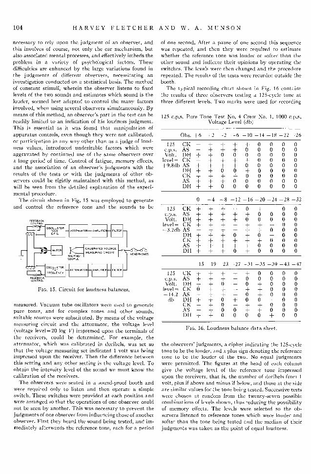
104 HARVEY FLETCHER AND W. A. MUNSON
necessary to rely upon the judgment of an observer, and this involves of course, not only the ear mechanism, but also associated mental processes, and effectively hnbeds the problem in a variety of psychological factors. Thesc difficulties are enhanced by the large variations found in the judgments of different observers, necessitating an investigation conducted on a statistical basis. The method of constant stimuli, wherein the observer listens to fixed levels of the two sounds and estimates which sound is the
louder, seemed best adapted to control the many factors involved, when using several observers simultaneously. By means of this method, an observer's part in the test can be readily limited to an indication of his loudness judgment. This is essential as it was found that manipulation of apparatus controls, even though they were not calibrated, or participation in any way other than as a iudge of loud- ness values, introduced undesirable factors which were aggravated by continued use of the same observers over a long period of time. Control of fatigue, memory effects, and the association of an observer's judgments with the results of the tests or with the iudgments of Other ob- servers could be rigidly maintained with this method, as will be seen from the detailed explanation of the experi- mental procedure.
The circuit shown in Fig. 15 was employed to generate and control the reference tone and the sounds to be
FIG. 15. Circuit for loudness balances.
measured. Vacuum tube oscillators were used to generate pure tones, and for complex tones and other sounds, suitable sources were substituted. By means of the voltage measuring circuit and the attenuator, the voltage level (voltage level = 20 log V) impressed upon the terminals of the receivers, could be determined. For example, the attenuator, which was calibrated in decibels, was set so that the voltage measuring set indicated 1 volt was being impressed upon the receiver. Then the difference between this setting and any other setting is the voltage level. To obtain the intensity level of the sound we must know the calibration of the receivers.
The observers were seated in a sound-proof booth and were required only to listen and then operate a simple switch. These switches were provided at each position and were arranged so that the operations of one observer could not be seen by another. This was necessary to prevent the judgments of one observer from influencing those of another observer. First they heard the sound being tested, and im- mediately afterwards the reference tone, each for a period
of one second. After a pause of one second this sequence was repeated, and then they were required to estimate whether the reference tone was louder or softer than the
other sound and indicate their opinions by operating the switches. The levels were then changed and the procednre repeated. The results of the tests were recorded outside the booth.
The typical recording chart shown in Fig. 16 contains the results of three observers testing a 12S-cycle tone at three different levels. Two marks were used for recording
125 c.p.s. Pure Tone Test No. 4 Crew No. 1. 1000 c.p.s. Voltage Level (db)
Obs. 4-6 4-2 -2 -6 -10 -14-18-22 -26
125 CK 4- + 4- 4- 4- 0 0 0 0 c.p.s. AS + + d- + 0 0 0 0 0 Volt. DH 4- 4- 0 0 0 0 0 0 0
level= CK + + + + + 0 0 0 0 4-9.8db AS 4- 4- 4- q- 0 0 0 0 0
DE[ 4- 4- 0 0 4- 0 0 0 0 CK + + + + 0 0 0 0 0 AS 4- 4- 4- 0 0 0 0 0 0 DH 4- + 0 0 0 0 0 0 0
0 --4 --8 --12 --16--20--24--28--32
125 CK 4- + 4- 4- 0 4- 4- 0 0 c.p.s. AS 4- 4- 4- 4- + 0 0 0 0 Volt. DH h- + 4- 4- 0 0 0 0 0
level= CK + + + + 4- + 4- 0 0 -3.2db AS 4- 4- h- h- 4- 4- 0 0 0
DH + h- h- 0 + 0 h- 0 0 CK + + + + + + 0 0 0 AS + + + + + 0 0 0 0 DH + + + 0 + 0 0 0 0
--15 --19 --23 --27 --31 --35 --39 --43 --47
125 CK h- h- h- h- + 0 0 0 0 c.p.s. AS + + + + 0 0 0 0 0 Volt. DH + + 0 + 0 + 0 0 0
level= CK 0 + + 4- + + 0 0 0 -14.2 AS + 4- + + 0 + 0 0 0
db DH + 4- 0 4- 0 0 4- 0 0 CK + + o + + + 0 0 0 AS + 4- 0 0 + + 0 0 0 DH 4- 4- 0 0 0 0 4- 0 0
Fm. 16. Loudness balance data sheet.
the observers' judgments, a cipher indicating the 125-cycle tone to be the louder, and a plus sign denoting the reference tone to be the louder of the two. No equal judgments were permitted. The figures at the head of each column give the voltage level of the reference tone impressed upon the receivers, that is, the number of decibels from 1 volt, plus if above and minus if below, and those at the side are similar values for the tone being tested. Successive tests were chosen at random from the twenty-seven possible combinations of levels shown, thus reducing the possibility of memory effects. The levels were selected so the ob- servers listened to reference tones which were louder and
softer than the tone being tested and the median of their judgments was taken as the point of equal loudness.
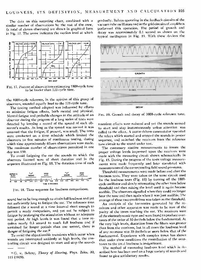
LOUDNESS, ITS DEFINITION, MEASUREMENT •ND C•LCULtkTION 105
The data on this recording chart, combined x•ith a similar number of observations by the rest of the crew, (a total of eleven observers) are shown in graphical form in Fig. 17. The arrow indicates the median level at which
vo,'r^Gd L•&-' 7 : _-c__
FIG. 17. Percent of obser• ations estimating 1000-cycle tone to be louder than 125-cycle tone.
gradually. Relays operating in the feedback circuits of the vacuum tube oscillators and in the grid circuits of anq)lifiers performed this operation. The period of grox•th and decay was approximately 0.1 second as ,own on the typical oscillogram in Fig. I9. \Vith these alex ices the
0 ! e'Ec
the 1000-c.xcle reference, in the opinion of this group of observers, sounded equally loud to the 12S-cycle tone.
The testing method adopted was influenced by efforts to minimize fatigue effects, both mental and physical. Mental fatigue and probable changes in the attitude of an observer during the progress of a long series of tests were detected by keeping a record of the spread of each ob- server's resttits. As long as the spread was normal it was assumed that the fatigue, if present, was small. The tests were conducted on a time schedule which limited the observers to five minutes of continuous testing, during which time approximately fifteen obserYations were made. The maximum number of observations permitted in one day was 150.
To avoid fatiguing the ear the sounds to which the observers listened were of short duration and in the seqnence illustrated on Fig. 18. The duration time of each
FIG. 18. Time sequence for loudness comparisons.
sound had to be long enough to attain full loudness and yet not sufficiently long to fatigue the ear. The refereuce tone followed the x sound at a time interval short enough to permit a ready comparison, and yet not be subject to fatigue by prolonging the stimulation without an adequate rest period. At high levels it was found that a tone re- quires nearly 0.3 second to reach full loudness anti if sustained for longer periods than one second, there is danger of fatiguing the ear. u
To avoid the objectionable transients which occur x• hen sounds are interrupted suddenly at high levels, the con- trolling circuit was designed to start and stop the sounds
n G. v. Bekesy, Theory of IIearing, Phys. Zeits. 30, 115 (1929).
DECAY
FXG. 19. Growth and decay of 1000-cycle reference tone.
transient effects were reduced anti yet the sotrods seemed to start and stop instantaneously unless attention was called to the effect. -k motor-driven commutator operated the relays which started and stopped the sountis in proper sequence, and sxGtched the receixers from the reference tone circuit to the sound under test.
The customary routine measurements to insure the proper voltage levels impressed upon the receivers were made with the measuring circuit shown schematically in Fig. 15. During the progress of the tests voltage measure- ments were made frequently and later correlated with measurements of the corresponding field sound pressures.
Threshold measurements were made before anti after the loudness tests. They were taken on the same circuit used for the loudness tests (Fig. 15) by turning off the 1000- cycle oscillator and slox• ly attenuating the other toue below threshold and then raising the level until it again became audible. The observers signalled when they could no longer hear the tone and then again when it was just amlible. The average of these two conditions was taken as the threshold.
An analysis of the harmonics generated by the re- ceivers and other apparatus was made to be sure of the purity of the tones reaching the ear. The receivers were of the electrodynamic type and • ere found to produce over- tones of the order of 50 decibels below the fundamental. At the very high lexels, distortion from the filters was greater than from the receivers, but in all cases the loudness level of any overtone was 20 decibels or more below that of the fundamental. Experience with complex tones has shown that under these comlitions the contribution of the over- tones to the total loudness is insignificant.
The method of measuring loudness level which is de. scribed here has been used on a large variety of sounds and found to give satisfactory rest, Its.
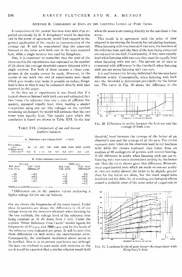
106 HARVEY FLETCHER AND W. A. MUNSON
APPENDIX B. COMPARISON OF DATA ON
A comparison of the present loudness data with that re- ported previously by B. A. Kingsbury 4 would be desirable and in the event of agreement, would lend support to the general application of the results as representative of the average ear. It will be remembered that the observers listened to the tones with both ears in the tests reported here, while a single receiver was used by Kingsbury.
Also, it is intportant to remember that the level of the tones used in the experiments was expressed as the number of db above the average threshold current obtained with a single receiver. For both of these reasons a direct com- parison of the results cannot be made. However, in the course of our work two sets of experiments were made which give results that make it possible to reduce Kings- bury's data so that it nray be compared directly with that reported in this paper.
In the first set of experiments it was found that if a typical observer listened with both ears and esti•nated that two tones, the reference tone and a tone of different fre- quency, appeared equally loud, then, nraking a similar comparison using one ear (the voltages on the receiver remaining unchanged) he would still estimate that the two tones were equally loud. The results upon which this conclusion is based are shown in Table XVI. In the first
TAnLE XVI. Comparison of one and two-ear loudness balances.
A. Reference tone voltage level --32rib
Frecluency, c.p.s. 62 i25 250 500 2000 4000 6000 8000 10,000
Voltage level difference* --0.5 0 +1.0 --1.0 --0.5 --0.5 4-0.5 --3.0 --3.0
B. Other reference tone levels
62 c.p.s. 2000 c.p.s. Ref. tone Volt. level Ref. tone Volt. level volt. level difference* volt. level difference*
-20 +0.5 -- 3 0.0 --34 +0.2 -22 +0.3 --57 +2.0 --41 --0.8 --68 --0.5 --60 --0.8
--7 ½ ) --6.2
* Differences are in (lb, positive values indicating a higher voltage for the one ear balance.
row are shown the frequencies of the tones tested. Under these frcquenciea are ahown the differences in db of the voitage levels on the receivers obtained when listening by the two methods, the voltage level of the reference tone being constant at 32 db down frmn I volt. Under the caption "Other Reference Tone Levels" similar figures for frequencies of 62 c.p.s. and 2000 c.p.s. and for the levels of the reference tone indicated are given. It will be seen that these differences are well within the observational error.
Consequently, the conclusion mentioned above seems to be justified. This is an important conclusion and although the data are confined to tests made with receivers on the
ear it would be expected that a similar relation would hold
1HE LOUDNESS LEVELS OF PURE TONES
when the sounds are coming directly to the ears from a free wave.
This result is in agreement with the point of view adopted in developing the formula for calculating loudness. When listening with one instead of two ears, the loudness of the reference tone and also that of the tone being compared are reduced to one-half. Consequently, if they were equally loud when listening with two ears they must be equally loud when listening with one ear. The second set of data is concerned with differences in the threshold when listening with one ear versus listening with two ears.
It is well known that for any individual the two ears have different acuity. Consequently, when listening with both ears the threshold is determined principally by the better ear. The curve in Fig. 20 shows the difference in the
•o so •oo zoo 500 •ooo zooo sooo ,oooo zoooo
F•o. 20. Difference in acuity between the best ear and the average of both ears.
threshold level between the average of the better of an observer's ears and the average of eli the ears. The. circles represent data taken on the observers used in our loudness tests while the crosses represent data taken from an analysis of 80 audiograms of persons with normal hearing. If the difference in acuity when listening with one ear rs. listening with two ears is determined entirely by the better ear, then the curve shown gives this difference. However, some experimental tests which we made on one ear acuity vs. two ear acuity showed the latter to be slightly greater than for the better ear alone, but the small magnitudes involved and the difficulty of avoiding psychological effects caused a probable error of the same order of magnitude as
Fro. 21. Loudness levels of pure tones--A comparison with Kingsbury's data.
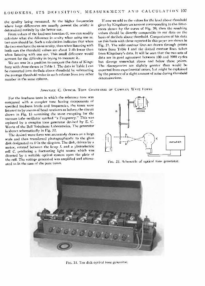
LOUDNESS, ITS DEFINITION, MEASUREMENT A\'D CALCULATION 107
the quality being measured. At the higher frequencies where large differences are usually present the acuity is deternfined entirely by the better ear.
From values of the loudness function G, one can readily calcnlate what the difference in acuity when using one z,s. two ears should be. Such a calculation indicates that when the two ears have the same acuity, then when listening with both ears the threshold values are about 2 db lower than when listening with one ear. This small difference would account for the difficulty in t%ing to measure it.
We are now in a position to compare the data of Kings- bury with those shown in Table I. The data in Table I can be converted into decibels above threshold by subtracting the average threshold value in each column frmn any other number in the same column.
If now we add to the values for the level above threshold given by Kingsbury an amount corresponding to the differ- ences shown by the curve of Fig. 20, then the resulting values should be directly comparable to our data on the basis of decibels above threshold. Comparisons of his data on this basis aith those reported in this paper are shown in Fig. 21. The solid contour lineq are drawn through points taken from Table I and the dotted contour linc• taken from Kingsbury's data. It will be seen that the txvo sets of data are in good agreement between 100 and 2000 cycles but diverge somexxhat above and below these points. The discrepancies are slightly greater than would be expected from experimental errors, but might be explained by the presence of a slight amount of noise during threshold deternfinations.
APPENDIX C. OPTICAL TONE (;ENER•,TOR OF COMPLEX. •V•,VE FORMS
For the loudness tests in which the reference tone was compared with a complex tone having components of specified loudness levels and frequencies, the tones were listened to by means of head receivers as before; the circuit shown in Fig. 15 remaining the same excepting for the vacuum tube oscillator marked "x Frequency." This was replaced by a complex tone generator dex iscd by E. C. Wente of the Bell Telephone Laboratories. The generator is shown schematically in Fig. 22.
The desired wave form was accurately drawn on a large scale and then transferred photographicalIs- to the glass disk designated as D in the diagram. The disk, driven by a motor, rotated between the lamp L and a photoelectric cell C, producing a fluctuating light source which was directed by a suitable optical system upon the plate of the cell. The voltage generated was alnplified and attenu- ated as in the case of the pure tones.
FIG. 22. Schematic of optical tone generator.
FIG. 23. Ten disk optical tone generator.
108 HARVEY FLETCHER AND W. A. MUNSON
The relative magnitudes of the components were of course fixed by the form of the wave inscribed upon the disk, but this was modified when desired, by the insertion of elements in the electrical circuit which gave the desired characteristic. Greater flexibility in the control of the amplitude of the components was obtained by inscribing each component on a separate disk with a complete optical system and cell for each. Frequency and phase relations were maintained by mounting all of the disks on a single shaft. Such a generator having ten disks is shown in Fig. 23.
An analysis of the voltage output of the optical tone generators showed an average error for the amplitude of the components of about 4-0.5 db, which was probably the linfit of accuracy of the measuring instrument. Undesired harmonics due to the disk being off center or inaccuracies in the wave form were removed by filters in the electrical circuit.
All of the tests on complex tones described in this paper were made with the optical tone generator excepting the audiometer, and two tone tests. For the latter tests, two vacuum tube oscillators were used as a source.