louise smy phd thesis - university of st andrews · · 2016-03-28a thesis submitted for the...
TRANSCRIPT

ATMOSPHERIC TRANSPORT AND CRITICAL LAYER MIXING INTHE TROPOSPHERE AND STRATOSPHERE
Louise Ann Smy
A Thesis Submitted for the Degree of PhDat the
University of St. Andrews
2012
Full metadata for this item is available inResearch@StAndrews:FullText
at:http://research-repository.st-andrews.ac.uk/
Please use this identifier to cite or link to this item:http://hdl.handle.net/10023/2538
This item is protected by original copyright

Atmospheric Transport and Critical Layer
Mixing in the Troposphere and Stratosphere
Louise Ann Smy
A thesis submitted for the degree of Doctor of Philosophy at the
University of St Andrews
25th October 2011

Abstract
This thesis aims to improve the understanding of transport and critical layer
mixing in the troposphere and stratosphere. A dynamical approach is taken
based on potential vorticity which has long been recognised as the essential field
inducing the flow and thermodynamic structure of the atmosphere. Within the
dynamical framework of critical layer mixing of potential vorticity, three main
topics are addressed.
First, an idealised model of critical layer mixing in the stratospheric surf
zone is examined. The effect of the shear across the critical layer on the criti-
cal layer evolution itself is investigated. In particular it is found that at small
shear barotropic instability occurs and the mixing efficiency of the critical layer
increases due to the instability. The effect of finite deformation length is also
considered which extends previous work.
Secondly, the dynamical coupling between the stratosphere and troposphere
is examined by considering the effect of direct perturbations to stratospheric
potential vorticity on the evolution of midlatitude baroclinic instability. Both
zonally symmetric and asymmetric perturbations to the stratospheric potential
vorticity are considered, the former representative of a strong polar vortex, the
latter representative of the stratospheric state following a major sudden warming.
A comparison of these perturbations gives some insight into the possible influence
of pre or post-sudden warming conditions on the tropospheric evolution.
i

Finally, the influence of the stratospheric potential vorticity distribution on
lateral mixing and transport into and out of the tropical pipe, the low lati-
tude ascending branch of the Brewer-Dobson circulation, is investigated. The
stratospheric potential vorticity distribution in the tropical stratosphere is found
to have a clear pattern according to the phase of the quasi-biennial oscillation
(QBO). The extent of the QBO influence is quantified, by analysing trajectories
of Lagrangian particles using an online trajectory code recently implemented in
the Met Office’s Unified Model.
ii

Acknowledgements
Firstly, I would like to thank my partner Nicholas Owen and both our families
for their endless love and support throughout my PhD.
Thanks to my supervisor Richard Scott for all the help, advice and encour-
agement that he has given me throughout my PhD. I would also like to thank the
Earth System and Mitigation Science team at the Met Office in Exeter for making
my visits there enjoyable. In particular I would like to thank Neal Butchart and
Steven Hardiman for all of their help throughout my time in Exeter and Steven
for his computing help whilst I was learning to run the Unified Model. I am also
grateful to Colin Johnson who helped me to write the code that retrieves the
fields, neccessary to run the trajectory code, from the Unified Model.
Finally I would like to thank UK EPSRC who financially supported me
throughout this project (CASE/CNA/06/76).
iii

Declaration
1. Candidates declarations:
I, Louise Ann Smy, hereby certify that this thesis, which is approximately 35,000
words in length, has been written by me, that it is the record of work carried
out by me and that it has not been submitted in any previous application for a
higher degree.
I was admitted as a research student in September 2007 and as a candidate for
the degree of Doctor of Philosophy in September 2008; the higher study for which
this is a record was carried out in the University of St Andrews between 2007
and 2011.
Signature:.............................. Date: ..............
2. Supervisors declaration:
I hereby certify that the candidate has fulfilled the conditions of the Resolution
and Regulations appropriate for the degree of Doctor of Philosophy in the Uni-
versity of St Andrews and that the candidate is qualified to submit this thesis in
application for that degree.
Signature:.............................. Date: ..............
iv

3. Permission for electronic publication:
In submitting this thesis to the University of St Andrews I understand that I
am giving permission for it to be made available for use in accordance with the
regulations of the University Library for the time being in force, subject to any
copyright vested in the work not being affected thereby. I also understand that
the title and the abstract will be published, and that a copy of the work may
be made and supplied to any bona fide library or research worker, that my the-
sis will be electronically accessible for personal or research use unless exempt
by award of an embargo as requested below, and that the library has the right
to migrate my thesis into new electronic forms as required to ensure continued
access to the thesis. I have obtained any third-party copyright permissions that
may be required in order to allow such access and migration, or have requested
the appropriate embargo below.
The following is an agreed request by candidate and supervisor regarding the
electronic publication of this thesis:
(i) Access to printed copy and electronic publication of thesis through the Uni-
versity of St Andrews.
Signature of Candidate:..............................
Signature of Supervisor:..............................
Date: ..............
v
Contents
Abstract i
Acknowledgements iii
Declaration iv
1 Introduction 4
1.1 Structure of the Atmosphere . . . . . . . . . . . . . . . . . . . . . 4
1.2 The Governing Equations Of Atmospheric Motion . . . . . . . . . 6
1.3 Atmospheric Transport and Mixing . . . . . . . . . . . . . . . . . 9
1.3.1 Rossby Waves . . . . . . . . . . . . . . . . . . . . . . . . . 9
1.3.2 Rossby Wave Critical Layers . . . . . . . . . . . . . . . . . 11
1.3.3 Barotropic And Baroclinic Instability . . . . . . . . . . . . 13
1.3.4 Mixing And Transport Across The Tropopause . . . . . . . 16
1.3.5 Dynamical Structure Of The Winter Stratosphere . . . . . 17
1.4 Quantifying Mixing and Transport . . . . . . . . . . . . . . . . . 18
1.4.1 Calculation of Effective Diffusivity . . . . . . . . . . . . . 20
1.5 Outline of Thesis . . . . . . . . . . . . . . . . . . . . . . . . . . . 27
1

2 Mixing in a Rossby Wave Critical Layer 29
2.1 Introduction . . . . . . . . . . . . . . . . . . . . . . . . . . . . . . 29
2.2 Model Description . . . . . . . . . . . . . . . . . . . . . . . . . . 31
2.3 Critical Layer Evolution . . . . . . . . . . . . . . . . . . . . . . . 35
2.4 Evolution at Finite Deformation Length . . . . . . . . . . . . . . 40
2.4.1 The Basic State . . . . . . . . . . . . . . . . . . . . . . . . 40
2.4.2 Scaling of the Critical Layer Width . . . . . . . . . . . . . 45
2.5 Conclusions . . . . . . . . . . . . . . . . . . . . . . . . . . . . . . 47
3 The Influence of Stratospheric Potential Vorticity on Baroclinic
Instability 49
3.1 Introduction . . . . . . . . . . . . . . . . . . . . . . . . . . . . . . 49
3.2 Model description . . . . . . . . . . . . . . . . . . . . . . . . . . . 53
3.3 Results . . . . . . . . . . . . . . . . . . . . . . . . . . . . . . . . . 60
3.3.1 Control . . . . . . . . . . . . . . . . . . . . . . . . . . . . 60
3.3.2 Zonally Symmetric Perturbation . . . . . . . . . . . . . . . 62
3.3.3 Asymmetric Perturbations . . . . . . . . . . . . . . . . . . 66
3.3.4 Influence of the basic state . . . . . . . . . . . . . . . . . . 72
3.4 Discussion . . . . . . . . . . . . . . . . . . . . . . . . . . . . . . . 76
4 An Online Trajectory Model 78
4.1 Offline trajectory code . . . . . . . . . . . . . . . . . . . . . . . . 78
4.2 Online trajectory code . . . . . . . . . . . . . . . . . . . . . . . . 81
4.3 Error Analysis . . . . . . . . . . . . . . . . . . . . . . . . . . . . . 83
2

5 The Effect of the Quasi-Biennial Oscillation on Transport and
Mixing in the Stratosphere 89
5.1 Introduction . . . . . . . . . . . . . . . . . . . . . . . . . . . . . . 89
5.2 The Effect of the Phase of the QBO on the Potential Vorticity
Structure . . . . . . . . . . . . . . . . . . . . . . . . . . . . . . . 96
5.2.1 The QBO . . . . . . . . . . . . . . . . . . . . . . . . . . . 96
5.2.2 Potential Vorticity Structure . . . . . . . . . . . . . . . . . 97
5.2.3 Experiment Design . . . . . . . . . . . . . . . . . . . . . . 102
5.3 Analysis of Trajectories . . . . . . . . . . . . . . . . . . . . . . . . 108
5.3.1 In-Mixing . . . . . . . . . . . . . . . . . . . . . . . . . . . 118
5.4 Discussion . . . . . . . . . . . . . . . . . . . . . . . . . . . . . . . 119
6 Conclusions 123
7 Appendix: Online Trajectory Code 128
7.1 Where to Find the Online Code and How to Use It . . . . . . . . 128
7.2 Information on Parameters . . . . . . . . . . . . . . . . . . . . . . 129
7.2.1 Particles Initial Positions . . . . . . . . . . . . . . . . . . . 131
7.3 Output . . . . . . . . . . . . . . . . . . . . . . . . . . . . . . . . . 132
Bibliography 135
3

Chapter 1
Introduction
The Earth’s atmosphere is a complex environment. The atmosphere contin-
ually strives to reach a state of equilibrium by transporting warm air from the
equator to the poles and cold air from the poles to the equator. At the same
time this movement of air is affected by the Earth’s rotation and friction at the
Earth’s surface. The combination of all these processes creates very complex
flow patterns and behaviour which requires extensive research to fully explore
and understand.
1.1 Structure of the Atmosphere
The atmosphere can be divided into layers based on its vertical temperature
profile. The layer nearest the Earth’s surface is known as the troposphere and it
extends from the ground up to between 8 and 16km. It is a region of particular
interest for meteorologists since most of our weather occurs here. The tropo-
sphere is a region of low stratification and weak potential vorticity (potential
vorticity can be interpreted as the absolute circulation divided by the mass of a
small volume enclosed between two isentropic surfaces). It is dynamically unsta-
4
ble due to baroclinic instability at middle latitudes (see section 1.3.3 for more
details on baroclinic instability) and due to convection in the tropics (Shepherd,
2002). Therefore transport time-scales in the troposphere are reasonably fast and
are typically a matter of hours for convective transport or a matter of days for
baroclinic transport (transport due to baroclinic instability). The temperature
in the troposphere decreases with height by an average of 7C per km (Burroughs
et al., 1996) reaching its coldest point at the thermal tropical tropopause. The
tropopause is defined as the notional boundary between the troposphere and the
stratosphere (the second layer of the atmosphere). Conventionally the tropopause
is defined, in terms of the thermal structure of the atmosphere, as the level where
there is an abrupt change in the temperature lapse rate (Andrews et al., 1987). A
dynamical tropopause is defined based on the jump in potential vorticity between
the troposphere and stratosphere (stratospheric potential vorticity is two orders
of magnitude greater than tropospheric potential vorticity). The height of the
tropopause varies with the amount of solar energy that reaches the Earth and
therefore it is lowest at the poles and highest at the equator. The tropopause
plays a crucial role in understanding the dynamics of the atmosphere (Haynes
et al., 2001).
The second layer of the atmosphere is the stratosphere which extends from
the tropopause up to approximately 50km. In contrast to the troposphere, which
is rather moist, the stratosphere is quite dry. The distribution of water vapour
along with carbon dioxide and ozone are responsible for the thermal structure
of the stratosphere by absorption of solar radiation. As the name suggests, the
stratosphere is strongly stably stratified as a result of the increase in temperature
with height. The dominant motions in the stratosphere are quasi-horizontal due
to this strong stable stratification. The temperature in the stratosphere reaches
a maximum at the stratopause (the “boundary” between the stratosphere and
the mesosphere, the third layer in the atmosphere) due to the absorption of solar
5

ultraviolet radiation by ozone (Andrews et al., 1987). In the mesosphere (50
to 80km) the concentration of ozone decreases reducing the absorption of solar
ultraviolet radiation and consequently the temperature decreases with height. In
the mesosphere the main dynamics are due to gravity wave breaking. Gravity
waves are waves that only exist in a stably stratified fluid and their restoring
force is due to gravity (e.g. buoyancy).
In this thesis we focus on the dynamics of the first two layers of the atmo-
sphere, namely the troposphere and stratosphere.
1.2 The Governing Equations Of Atmospheric
Motion
In order to model the atmosphere we need to understand the equations that
govern atmospheric motion and then solve these simultaneously. The full equa-
tions are far too complicated to be used for research purposes and so we simplify
them using many standard approximations.
The Equation of Motion (or Conservation of Momentum), assuming that vis-
cous effects are negligible, the fluid is incompressible (∇ · u = 0) and the hor-
izontal length scales are much smaller than the curvature of the Earth (f-plane
approximation), is detailed below
Du
Dt+ fk × u = −
∇p
ρ−∇φ (1.1)
where u is the velocity,D
Dtdenotes the material derivative i.e.
∂
∂t+ u · ∇ , the
vector quantity fk is known as the “planetary vorticity” where f = 2Ωsinφ is
the coriolis frequency and denotes the vertical component of the Earth’s rotation
vector (Ω), and k denotes the local vertical unit vector. This equation represents
6

Newton’s second law of motion which is the balance between force (in this case
centrifugal force, coriolis force, pressure force and gravity) and acceleration. Here
the centrifugal force is absorbed into the geopotential term (φ = gz− 12Ω2(x2+y2),
where g is the acceleration due to gravity).
The Continuity Equation (or Conservation of Mass)
∂ρ
∂t+ ∇ · (ρu) = 0 (1.2)
where ρ is density. This states that mass is neither created nor destroyed in a
material volume.
A Thermodynamic Equation such as conservation of entropy
Dθ
Dt= 0 (1.3)
where θ = T (ps/p)κ is the potential temperature distribution (functionally related
to entropy). Here T is the temperature, p is pressure, ps is a reference surface
pressure and κ = 2/7 for the atmosphere.
An Equation of State for an ideal gas
p = ρRT (1.4)
where R is the gas constant for dry air.
A quantity of dynamical importance is Ertel’s potential vorticity which is
defined, following the same approximations as for the Equation of Motion, by
EPV = ρ−1ωa · ∇θ (1.5)
where ωa = ∇×u+fk is the absolute vorticity. Potential vorticity has long been
recognised as the essential field inducing the flow and thermodynamic structure
7
of the atmosphere. Moreover, it is materially conserved (i.e. following the motion
of fluid elements) in adiabatic and inviscid flows. Hence many aspects of geophys-
ical flows can be described compactly in terms of potential vorticity (a scalar)
dynamics (Hoskins et al., 1985; Schneider et al., 2003). The “invertibility princi-
ple” states that if the total mass under each isentropic surface is specified, then a
knowledge of the global distribution of potential vorticity on each isentropic sur-
face (surface of constant potential temperature, θ) and of potential temperature
at the lower boundary (which within certain limitations can be considered to be
part of the potential vorticity distribution (Bretherton, 1966)) is sufficient to de-
duce, diagnostically, all the other dynamical fields, such as winds, temperatures,
geopotential heights, static stabilities, and vertical velocities, under a suitable
balance condition (Andrews et al., 1987). In this thesis we examine the structure
of potential vorticity in a variety of different models and stratospheric contexts.
Using the standard approximations for rapidly rotating and strongly stratified
flows, i.e. taking the Rossby number Ro = ζ/f (ζ denotes the vertical vorticity,∂v
∂x−∂u
∂y)and the Froude number Fr = |ωh|/N (ωh denotes the horizontal vor-
ticity, (∇× u)h and N is the buoyancy frequency) both much less than one, we
arrive at the quasi-geostrophic equations (or QG equations for short). These can
be written in the following convenient form:
DhQ
Dt= 0 (1.6)
where Q is the quasi-geostrophic potential vorticity which is conserved following
motion andDh
Dt=
∂
∂t+ u
∂
∂x+ v
∂
∂y. Note that the velocity in the material
derivative is the geostrophic velocity. The quasi-geostrophic potential vorticity is
related to a streamfunction ψ by the linear “inversion relation”
Q− f = ∇h2ψ +
1
ρ0
∂
∂z
(
ρ0f 2
N2
∂ψ
∂z
)
(1.7)
8

where ψ =p′
ρ0f(from geostrophic balance), p′ is the pressure perturbation, f is
the Coriolis frequency, N is the buoyancy frequency, and ∇h2 is the horizontal
Laplacian. Here p′ is the total pressure minus the basic-state pressure p0(z),
and ρ0(z) = ρs exp(−z/Hρ) is the basic-state density, where ρs is a reference
surface density andHρ is the “density scale height”, above 7km in the atmosphere
(Andrews et al., 1987). Note, in general N2 varies with height z.
From the streamfunction ψ, the two-dimensional flow field is recovered from
(u, v) =
(
−∂ψ
∂y,∂ψ
∂x
)
. (1.8)
1.3 Atmospheric Transport and Mixing
1.3.1 Rossby Waves
One of the most important dynamical properties of the atmosphere is its
ability to support wave motions. Rossby waves are the fundamental building
blocks of weather systems at midlatitudes. They are potential vorticity conserving
motions that exist wherever there are large-scale potential vorticity gradients
along isentropic surfaces (surfaces of constant potential temperature, θ). Rossby
waves are often large-scale waves (i.e. large wavelength) so much so that typically
they only have a few wavelengths around the whole of the Earth (Kundu & Cohen,
2004).
The dynamical mechanism of Rossby waves and Rossby wave propagation is
a restoring mechanism that depends on the existence of a latitudinal gradient of
potential vorticity on isentropic surfaces. Figure 1.1 shows a schematic of Rossby
wave propagation on a material contour separating an area of high potential vor-
ticity from an area of low potential vorticity. The material contour is perturbed
9

and this results in positive and negative potential vorticity anomalies, the circu-
lations of which are indicated by the green arrows in Figure 1.1. The circulations
of these anomalies cause part of the material contour to move polewards and part
to move equatorwards. This movement is indicated by the double blue arrows
in Figure 1.1 and this results in the westward movement of the wave pattern.
Therefore Rossby waves propagate westward.
The depth of the atmosphere is very small compared to its horizontal scale.
The trajectories of particles in the atmosphere are very shallow with the hor-
izontal velocities being much larger than the vertical velocities. The effect of
the rapid rotation of the Earth and the strong stratification in the stratosphere
is to ensure vertical velocities are significantly smaller than horizontal velocities
and therefore a two dimensional approximation is a reasonable one for describing
large-scale motions.
The dispersion relation for a Rossby wave in two dimensions is given by
ω = −βk
k2 + l2(1.9)
where k and l are the x and y wavenumbers respectively and β =∂f
∂yis the rate
of change of the Coriolis parameter with y. The phase speed of the Rossby wave
is
c =ω
k= −
β
k2 + l2(1.10)
The negative in (1.10) is consistent with the Rossby wave phase propagation
being westward.
In the atmosphere Rossby waves often exist where there is an eastward mean
background flow (let’s denote the speed of the mean flow by U). When this occurs
the observed phase speed of the Rossby wave is
10

y
pole
equator
HIGH PV
LOW PV
material contour
Figure 1.1: Schematic of Rossby wave propagation on a material contour.
c = U −β
k2 + l2(1.11)
It is therefore possible to have stationary Rossby waves and they occur when
the eastward mean background flow equals the westward phase speed resulting
in c = 0.
1.3.2 Rossby Wave Critical Layers
Rossby waves propagate through a medium with a phase speed c. A critical
surface (or critical line in two dimensions) occurs where the speed of the back-
ground flow equals the phase speed of the Rossby wave. Nonlinear effects become
important in the region surrounding the critical surface (or critical line) and this
region is known as a Rossby wave critical layer.
The evolution within the critical layer is characterised by the wrapping up
of material contours of potential vorticity into the well known cat’s eye pattern
(see Figure 1.2). This wrapping up of potential vorticity mixes potential vortic-
ity by moving low potential vorticity into areas of high potential vorticity and
high potential vorticity into areas of low potential vorticity. After some time a
zonal average of the potential vorticity will reveal that the potential vorticity is
11

Figure 1.2: Snapshot of potential vorticity contours wrapping up into a cat’s eye
pattern.
homogenised across the critical layer region.
The study of critical layers goes back to the work of Benney & Bergeron
(1969), Davis (1969), Dickinson (1970) and other authors. A significant advance
in the theory of critical layers was made by the analytical work of Stewartson
(1978) and Warn & Warn (1978) (hereafter SWW). They forced Rossby waves by
flow over a corrugated boundary and applied the method of matched asymptotic
expansions to the resulting critical layer. The critical layer was treated as the in-
ner region in this analytical approach. A complete analytical solution was found
for a particular choice of boundary conditions and this allowed accurate predic-
tions to be made about the time evolution of the critical layer. One interesting
prediction of the SWW solution concerned the wave motion outside the critical
layer. The critical layer exerts its influence on the flow outside the critical layer
and oscillates between a wave absorber (absorbs energy from incident Rossby
waves) and an over-reflector (reflects the incoming wave and releases some of the
wave activity previously absorbed). In the long-time limit the critical layer tends
to a state of perfect reflection. The absorbing and reflecting properties of critical
layers was examined further by Killworth & McIntyre (1985).
The study of critical layers is important for understanding large-scale atmo-
12

spheric flows. The theoretical models of Rossby wave critical layers predicted be-
haviour that was in broad agreement with the wave breaking structures observed
by McIntyre & Palmer (1983, 1984) in coarse-grain maps of potential vorticity on
isentropic surfaces in the northern winter hemisphere stratosphere. These maps
of potential vorticity on isentropic surfaces made the large-scale wave breaking in
the surf zone visible for the first time. In particular these maps showed the rapid
and irreversible deformation of material contours along isentropic surfaces which
was predicted by the theoretical models of critical layers. Therefore the study of
critical layers is important for understanding Rossby wave breaking events in the
atmosphere. The study of critical layers is also important for understanding the
banded structures observed in our atmosphere and the atmosphere of Jupiter.
Critical layers mix potential vorticity across the critical layer region leading to
strong potential vorticity gradients on either side of the critical layer resembling
a potential vorticity staircase (McIntyre, 1982). Critical layer mixing is therefore
important for jet sharpening and recent work has focussed on the link between
potential vorticity mixing and jet sharpening (Dritschel & McIntyre, 2008).
1.3.3 Barotropic And Baroclinic Instability
There are two types of instability that are important in the atmosphere,
barotropic and baroclinic instability. An atmosphere, or model, is barotropic
if the pressure only depends on the density and therefore surfaces of constant
pressure are parallel to surfaces of constant density. The large-scale motion in
a barotropic model is horizontal and does not depend on the structure in the
vertical. Barotropic instability can be thought of as a horizontal shear instabil-
ity. It occurs where there is non-monotonic potential vorticity, i.e. the potential
vorticity gradient changes sign in the horizontal domain (which is dynamically
unstable, (Drazin & Reid, 2004)).
13

In contrast to barotropic instability baroclinic instability can be thought of
as a vertical shear instability (opposite signs of the latitudinal potential vorticity
gradient on the upper and lower levels). In a baroclinic atmosphere, or model,
density depends on both the pressure and the temperature. In the troposphere the
dominant dynamics are due to baroclinic instability. We can think of baroclinic
instability arising from the interaction of two Rossby waves, one at the tropopause
and one at the Earth’s surface (see Figure 1.3). At the surface the temperature
gradient is equivalent to a negative potential vorticity gradient, i.e. it is opposite
to the potential vorticity gradient at the tropopause. This results in the surface
Rossby waves propagating eastward. There is a vertical shear associated with
the surface temperature gradient (warm at the equator and cold at the pole due
to the pole-equator difference in solar heating). The relationship between the
vertical shear and the horizontal temperature gradient is given by the equation
of thermal wind balance
(
∂T
∂y= −
∂u
∂z
)
which is a direct result of hydrostatic
and geostrophic balance in the atmosphere. Due to the vertical shear in the
troposphere the two Rossby waves, which otherwise move in opposite directions,
can become phase locked. The winds strengthen in the eastward direction with
increasing height due to the vertical shear. The Rossby waves at the tropopause
are propagating westward with respect to the flow. However relative to the
surface the Rossby waves (at the tropopause) propagate with a speed equal to
their phase speed plus the background velocity. Therefore if the vertical shear is
strong enough the Rossby waves (at the tropopause) will move eastwards relative
to the surface which is the same direction as the surface Rossby waves. These
waves can then become phase locked, keeping each other in step and if the phase
is correct then the circulation of the upper potential vorticity anomalies will have
an effect on the surface potential vorticity anomalies and vice versa. In this way
they cause each other to grow in amplitude until they become nonlinear where
they saturate and break (flow instability).
14

tropopause
surfacey
y
pole
equator
pole
equator
HIGH PV
LOW PV
LOW PV
HIGH PV
zvertical shear
Figure 1.3: Schematic of the interaction of two Rossby waves: one at the
tropopause and one at the surface.
15

The baroclinic eddies generated via the instability due to Rossby wave phase
locking grow by extracting energy from the mean flow which is associated with
the pole-equator difference in solar heating. The eddies thus generated give rise to
our midlatitude weather systems and are mainly responsible for the atmospheric
heat transport from the tropics to midlatitudes.
1.3.4 Mixing And Transport Across The Tropopause
Mixing and transport across the tropopause is important for understanding
the distributions of chemical constituents in the troposphere and stratosphere and
their consequent effects on the atmosphere, for example its thermal structure and
ozone depletion.
There are many processes that contribute to transport across the tropopause.
The Brewer-Dobson circulation, named after the pioneering work of Alan Brewer
(1949) and Gordon Dobson (1956), is a large-scale middle atmosphere circula-
tion. It is responsible for the long-time persistent transport of air and chemi-
cal constituents from the troposphere into the stratosphere through the tropical
tropopause (for more details on the Brewer-Dobson circulation see chapter 5).
Air in the tropical troposphere is drawn upwards by the Brewer-Dobson circu-
lation, it expands due to the reducing pressure with increasing height and this
expansion results in the temperature of the air decreasing (note that for adiabatic
motion the temperature lapse rate is given by − gcp
where g is gravity and cp is the
specific heat capacity). Where this reduction in temperature, due to ascent, is
strongest is known as the thermal tropical tropopause or cold trap. Air passing
through the thermal tropical tropopause is dehydrated by the condensation of
water vapour. Dehydration of air entering the stratosphere influences the distri-
bution of water vapour in this atmospheric layer. Another consequence of the
transport of chemicals into the stratosphere by the Brewer-Dobson circulation is
16

that some of these chemicals (e.g. CFCs) are involved in processes such as ozone
destruction.
At middle latitudes transport across the tropopause is predominantly due to
tropopause folding. Tropopause folding is a process in which the tropopause
(defined in terms of potential vorticity) intrudes deeply into the troposphere
(Andrews et al., 1987). This results in high potential vorticity air from the
stratosphere entering the troposphere and then being mixed with tropospheric
air along the edges of the tropopause fold. Tropopause folds are responsible for
transport of air from the stratosphere into the troposphere.
1.3.5 Dynamical Structure Of The Winter Stratosphere
In the winter stratosphere potential vorticity on isentropic surfaces is high at
the pole and low in the tropics. The winter polar stratosphere is dominated by the
polar vortex. Due to cooling over the winter pole (the winter pole is tilted away
from the sun) there is a strong eastward flow around the pole in the stratosphere
which is the polar vortex. This situation allows the propagation of planetary scale
Rossby waves from the troposphere into the stratosphere (Charney & Drazin,
1961). Rossby waves are excited by flow over topography (e.g. Himalayas, Rocky
Mountains) and by land-sea temperature contrasts. These waves propagate up
from the troposphere and break in a region of the stratosphere known as the surf
zone (McIntyre, 1982; McIntyre & Palmer, 1983, 1984). The surf zone is a large
Rossby wave critical layer (see chapter 2 for more details on critical layers) and
when Rossby wave breaking occurs it mixes air isentropically over large areas of
the stratosphere.
Very large amplitude wave breaking on the edge of the polar vortex is known
as a stratospheric sudden warming. In a stratospheric sudden warming the wave
breaking, due to its large amplitude, typically leads to a breakdown of the po-
17

lar vortex. Stratospheric sudden warmings mix cold polar air equatorward and
warmer midlatitude air poleward and therefore have a significant impact on the
temperature at the pole and the distribution of chemicals, such as ozone, in the
stratosphere.
The dynamical structure of the stratosphere is characterised by strong gradi-
ents of potential vorticity in the subtropics and at polar latitudes. These strong
potential vorticity gradients are formed by mixing in the stratospheric surf zone
which steepens the potential vorticity gradients in these two regions and weakens
potential vorticity gradients in the surf zone resulting in a potential vorticity stair-
case profile (McIntyre, 1982). Strong gradients of potential vorticity are barriers
to mixing and transport and therefore these potential vorticity gradients isolate
air in the tropics and at the poles from the vigorous mixing of the extratropical
surf zone.
Several studies have examined mixing and transport across the subtropical
barrier, for example Plumb (1996), Neu & Plumb (1999), Ray et al. (2010).
Mixing and transport into the tropics has significant implications for tracer con-
centrations within the stratosphere.
1.4 Quantifying Mixing and Transport
Mixing of a fluid is a result of advection (“stirring”), which stretches and folds
material contours, and also of diffusion, which is an irreversible process. There
are several diagnostics that can be used to quantify the mixing and transport
properties of a given fluid flow. Mixing and transport can be measured directly
by analysing the movement of particles in Lagrangian trajectories (see chapter
5).
Lagrangian measures such as Lyapunov exponents and contour lengths can
18

be used to quantify mixing. Lyapunov exponents characterise the average rate
of separation of particles in a flow. If δx0 denotes the separation of two particles
at time t = t0 their separation after some time t is given by
|δx(t)| = eλt|δx0| (1.12)
where λ is the Lyapunov exponent. Contour lengths are also a good measure of
mixing. The length of a material contour is greater than its initial length when
it has been stretched and folded due to stirring. As a result of this stirring there
is more contour interface for diffusion to act upon which enhances the mixing.
Effective diffusivity (κeff) as described by Nakamura (1996) is a hybrid Eulerian-
Lagrangian quantity and is a useful diagnostic for calculating the mixing prop-
erties of a given flow. Effective diffusivity is a measure of how much more a
tracer particle, say, has been transported compared to how it would have moved
due to molecular diffusion alone. Calculating the effective diffusivity comes from
transforming the advection-diffusion equation (1.13) to tracer coordinates, using
a mapping between tracer concentration and area, to give a diffusion only equa-
tion (see section 1.4.1). Another diagnostic linked to the effective diffusivity is
the equivalent length (Le). Equivalent length is related to the contour length in
that it increases as contours are stretched and folded due to stirring.
Nakamura (1996), Haynes & Shuckburgh (2000a) and Haynes & Shuckburgh
(2000b) have shown the usefulness of effective diffusivity as a diagnostic of mixing.
In particular Shuckburgh & Haynes (2003) show that effective diffusivity can
be used as a quantitative diagnostic of transport and mixing with their results
illustrating how effective diffusivity accurately captures the location and character
of barrier and mixing regions.
Effective diffusivity has been used to examine mixing in the upper tropo-
sphere and lower stratosphere (Scott et al., 2003). It was found that the sub-
19

γ(C, t)
∇c
uC
y
x
C
C’
c(x,y,t)
A(C,t)
dC
ds
Figure 1.4: Diagram of the area coordinate. It shows 2 contours C of the tracer
c(x, y, t) with the area A(C, t) being that enclosed above the contours.
tropical tropopause was a region of low effective diffusivity suggesting that it
acts as a partial barrier to the transport of particles from the troposphere into
the stratosphere. More recently effective diffusivity has also been used to inves-
tigate two-dimensional mixing and transport in idealised hurricane-like vortices
(Hendricks & Schubert, 2009).
1.4.1 Calculation of Effective Diffusivity
In order to calculate the effective diffusivity (i.e. transforming the advection-
diffusion equation (1.13) to a diffusion only equation) it is useful to begin by
considering the evolution of a passive tracer in a given flow. The advection-
diffusion equation for a passive tracer in an incompressible flow (∇ · u = 0) is
∂c
∂t+ u · ∇c = ∇ · (κ∇c) (1.13)
where c(x, y, t) is the concentration of the passive tracer and κ is the constant
diffusivity.
This advection-diffusion equation (1.13) can be reduced to a diffusion only
20

equation by making a transformation from Cartesian coordinates (x, y) to tracer
coordinates (C, s) (following Nakamura (1996) and Hendricks & Schubert (2009)).
C represents a given value of the passive tracer c(x, y, t), γ(C, t) is defined as the
contour enclosing all the tracer where c(x, y, t) ≥ C and s is the position on the
contour γ(C, t). Let the region enclosed by the contour γ(C, t) be denoted by
A(C, t) so that
A(C, t) =
∫ ∫
c≥C
dxdy (1.14)
Note that as the value of C increases, the area enclosed by C decreases (i.e.
A(C, t) is a monotonically decreasing function of C) with A(Cmax, t) = 0.
Let uC be the velocity of the contour γ(C, t) and define it such that
∂c
∂t+ uC · ∇c = 0 (1.15)
This is not a unique definition. Note that the contour γ(C, t) is not a material
contour since diffusion allows fluid to move across the contour. However uC is the
velocity of the contour, not the fluid velocity, and therefore γ(C, t) is a material
contour w.r.t. uC .
As the contour γ(C, t) moves in time, we want an expression for the rate of
change of the area, A(C, t), enclosed by this contour. The rate of change of area
is the circumference of the contour γ(C, t) multiplied by the normal component
of the velocity of the contour, uC .
∂A(C, t)
∂t=
∂
∂t
∫ ∫
c≥C
dxdy = −
∫
γ(C,t)
uC ·∇c
| ∇c |ds (1.16)
Note that the normal is the outward normal and ∇c is inward. Therefore the
normal is −∇c
| ∇c |.
21

Now substituting (1.15) into (1.13) we can write uC in terms of the fluid
velocity u as follows
uC · ∇c = u · ∇c−∇ · (κ∇c) (1.17)
Substituting this into the last equality of (1.16) produces
∂A(C, t)
∂t=
∫
γ(C,t)
∇ · (κ∇c)ds
| ∇c |−
∫
γ(C,t)
u · ∇cds
| ∇c |(1.18)
The second term on the right hand side of (1.18) is an advection term and
can be written as
−
∫
γ(C,t)
∇ · (cu)ds
| ∇c |(1.19)
using u · ∇c = ∇ · (cu) for an incompressible flow.
In order to take the factor c outside the integrand and therefore have ∇ ·
u = 0, thus making the whole term zero, we need to transform (1.19) into a
surface integral and then back to a line integral using the divergence theorem
(∫∫
A∇ · F dA =
∫
γF · ds).
The area element in Cartesian coordinates is dA = dxdy. In tracer coordinates
dA =dsdC ′
| ∇c |where
1
| ∇c |is the Jacobian for the transformation from Cartesian
coordinates to tracer coordinates. Therefore
∂
∂C
∫ ∫
c≥C
(....)dxdy =∂
∂C
∫ ∫
c≥C
(....)dsdC ′
| ∇c |= −
∫
γ(C,t)
(....)ds
| ∇c |(1.20)
The last equality comes from the use of first principles to write the derivative in
the limit C −→ 0.
Now reading (1.20) in reverse and substituting into (1.19) yields
22
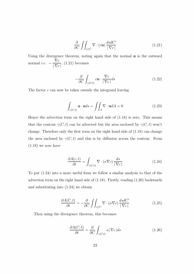
∂
∂C
∫ ∫
c≥C
∇ · (cu)dsdC ′
| ∇c |(1.21)
Using the divergence theorem, noting again that the normal n is the outward
normal i.e. −∇c
| ∇c |, (1.21) becomes
−∂
∂C
∫
γ(C,t)
cu ·∇c
| ∇c |ds (1.22)
The factor c can now be taken outside the integrand leaving
∫
γ(C,t)
u · nds =
∫ ∫
A
∇ · udA = 0 (1.23)
Hence the advection term on the right hand side of (1.18) is zero. This means
that the contour γ(C, t) can be advected but the area enclosed by γ(C, t) won’t
change. Therefore only the first term on the right hand side of (1.18) can change
the area enclosed by γ(C, t) and this is by diffusion across the contour. From
(1.18) we now have
∂A(c, t)
∂t=
∫
γ(C,t)
∇ · (κ∇c)ds
| ∇c |(1.24)
To put (1.24) into a more useful form we follow a similar analysis to that of the
advection term on the right hand side of (1.18). Firstly, reading (1.20) backwards
and substituting into (1.24) we obtain
∂A(C, t)
∂t= −
∂
∂C
∫ ∫
c≥C
∇ · (κ∇c)dsdC ′
| ∇c |(1.25)
Then using the divergence theorem, this becomes
∂A(C, t)
∂t=
∂
∂C
∫
γ(C,t)
κ| ∇c |ds (1.26)
23

To examine mixing and transport in a fluid we want to know how the value of
tracer enclosing a given area, A, changes in time . The area A(C, t) is a monotonic
(decreasing) function of tracer value C. This means that the inverse C(A, t) is
unique. Using the chain rule we obtain the following relation
∂A(C, t)
∂t
∂C(A, t)
∂A(C, t)= −
∂C(A, t)
∂t(1.27)
Substituting (1.27) into (1.26) produces
∂C(A, t)
∂t= −
∂C(A, t)
∂A
∂
∂C
∫
γ(C,t)
κ| ∇c |ds = −∂
∂A
∫
γ(C,t)
κ| ∇c |ds (1.28)
From (1.20), the integral on the right hand side of (1.28) can be written as
follows
∫
γ(C,t)
κ| ∇c |ds =
∫
γ(C,t)
κ| ∇c |2ds
| ∇c |= −
∂
∂C
∫ ∫
c≥C
κ| ∇c |2dxdy (1.29)
Substituting this into (1.28), we obtain
∂C(A, t)
∂t=
∂
∂A
(
∂
∂C
∫ ∫
c≥C
κ| ∇c |2dxdy
)
(1.30)
This can be rewritten to the form
∂C(A, t)
∂t=
∂
∂A
(
Keff(A, t)∂C(A, t)
∂A
)
(1.31)
where
Keff(A, t) =
(
∂C(A, t)
∂A
)−2∂
∂A
∫ ∫
c≥C
κ| ∇c |2dxdy (1.32)
24

Therefore, using the area coordinate, the advection-diffusion equation (1.13)
has become a diffusion-only equation (1.31). The effective diffusivity defined by
(1.32) is a useful diagnostic of mixing and transport in a fluid. It has been shown
by Shuckburgh & Haynes (2003) to capture the precise location and character
of mixing regions and barriers to transport within a flow. Note, however, that
the effective diffusivity does not have the normal dimensions of diffusion (m2s−1)
but rather the dimensions m4s−1. This is due to the use of the area coordinate.
In order for the effective diffusivity to have more convenient dimensions, i.e.
those of normal diffusion, (1.32) can be rewritten replacing the area coordinate
A with either an equivalent radius coordinate, re, for cylindrical geometry or an
equivalent latitude coordinate, ye, for channel geometry.
Firstly consider an equivalent radius coordinate, re, for a cylindrical domain,
where
πre2 = A (1.33)
From (1.33) it can be seen that
1
2πre
∂
∂re=
∂
∂A(1.34)
Substituting this into (1.31) yields
∂C(re, t)
∂t=
1
re
∂
∂re
(
reκeff(re, t)∂C(re, t)
∂re
)
(1.35)
with
κeff(re, t) =Keff(A, t)
4πA(1.36)
Now, for mixing in a channel, we consider an equivalent latitude coordinate,
ye, where
25
Lxye = A (1.37)
Let the width of the channel be Lx = 2π. Then
2πye = A (1.38)
From this, it can be seen that
1
2π
∂
∂ye=
∂
∂A(1.39)
Substituting this into (1.31) produces
∂C(ye, t)
∂t=
∂
∂ye
(
yeκeff(ye, t)∂C(ye, t)
∂ye
)
(1.40)
with
κeff(ye, t) =Keff(A, t)
2πA(1.41)
Another equivalent diagnostic is equivalent length, defined as
Le(A, t)2 =
1
κKeff(A, t) (1.42)
The equivalent length is related to the length of the contour γ(C, t). Le ≥ L
always, where L is the length of the contour γ(C, t) enclosing a given tracer
value. Note that equality is achieved in the special case where ∇c = 0 along the
contour γ(C, t).
26

1.5 Outline of Thesis
In this thesis we investigate atmospheric transport and critical layer mixing
in the troposphere and stratosphere in a range of models, from very idealised
models through to a more realistic model of the atmosphere.
In chapter 2 we model critical layer mixing in a two dimensional channel and
investigate the effect of the background shear flow on the evolution of the flow
inside the critical layer, with particular attention to the occurrence of barotropic
instability. We also consider how the mixing efficiency depends on the shear
across the critical layer and we compare two different measures of mixing (effective
diffusivity and contour lengths). Consideration is also given to the effect of finite
Rossby deformation length on the critical layer evolution.
In chapter 3 we investigate how the location of the stratospheric polar vor-
tex affects the location of the critical layer on the subtropical jet and how this
then affects the dynamics in the troposphere. In particular we examine in detail
how a significant redistribution of the stratospheric potential vorticity, as is ob-
served during major stratospheric sudden warmings, can effect the evolution in
the troposphere and at the Earth’s surface.
Chapter 4 describes a trajectory model, developed in conjunction with the
UK Met Office, which will be used for the study of atmospheric transport and
mixing in more realistic situations. A brief outline of the model is given along
with the results of some sensitivity experiments.
In chapter 5 the trajectory model described in chapter 4 is used to investi-
gate the effect of the quasi-biennial oscillation (hereafter QBO) on mixing and
transport in the stratosphere. We form a hypothesis, of how the QBO may af-
fect mixing and transport, based on the potential vorticity structure. Here we
examine mixing and transport directly by analysing trajectories of Lagrangian
particles in order to test the hypothesis and determine if an effect exists. In
27

chapter 6 our findings throughout this thesis are summarised and discussed.
Finally chapter 7 contains the documentation for the trajectory model de-
scribed and used in chapters 4 and 5. It details where to find the code and how
to view the model output along with some information about specific parameters.
28

Chapter 2
Mixing in a Rossby Wave Critical
Layer
2.1 Introduction
Critical layers can be thought of as a model of Rossby wave breaking in the
stratosphere. The continued interest in the study of critical layers is invaluable
to aid the understanding of large scale atmospheric flows.
The equation for linear Rossby wave propagation on a non-uniform basic state
U(y) has a singularity at points y for which the Rossby wave phase speed c equals
the basic state: U−c = 0. In the vicinity of such points linear theory breaks down
and nonlinear terms in the governing equation must be retained. The region over
which where nonlinearity is important is referred to as a Rossby wave critical
layer. Within the critical layer the evolution is characterised by the wrapping
up of material contours of potential vorticity in the well known Kelvin cat’s
eye pattern. The cat’s eye evolution mixes potential vorticity inside the critical
layer. Critical layers are regions of great importance due to the strong mixing and
transport that occurs within them. Another important issue is whether critical
29

layers act as wave absorbers or reflectors (depending on the details of the mixing).
The study of critical layers goes back to the work of Benney & Bergeron
(1969), Davis (1969), Dickinson (1970) and other authors. A significant advance
in the theory of critical layers was made simultaneously by Stewartson (1978)
and Warn & Warn (1978) (hereafter SWW). They investigated analytically the
structure of the critical layer formed by forcing Rossby waves in a uniform shear
flow. SWW applied the method of matched asymptotic expansions to the problem
of Rossby wave critical layers and treated the critical layer as the inner region. An
exact analytical solution was found for a particular choice of boundary conditions.
The SWW solution for this special case allowed accurate predictions to be made
about the time evolution of the critical layer. One such prediction of the SWW
solution is that the critical layer oscillates between an absorbing state (absorbs
energy from incident Rossby waves) and an over-reflecting state (reflects the
incoming wave and releases some of the wave activity previously absorbed). In
the long-time limit the critical layer tends to a state of perfect reflection. The
absorbing and reflecting properties of critical layers was examined further by
Killworth & McIntyre (1985).
The work of SWW was extended by Haynes (1989). Haynes (1989) used a
generalisation of the SWW solution for the exact critical layer dynamics to ex-
plore the evolution of the critical layer over a range of the single non-dimensional
parameter which governed the system. Killworth & McIntyre (1985) have shown
that the SWW critical layer flow is unstable. In particular Haynes (1989) inves-
tigated the development of the instability within the critical layer and its effect
on the critical layer absorptivity. Haynes (1989) showed that the simple wrap-up
within the critical layer may break down due to barotropic instability in regions
where the potential vorticity is locally non-monotonic. This barotropic instabil-
ity makes a substantial difference to the potential vorticity distribution in the
critical layer. Haynes (1989) also found that the instability increased the time
30

integrated absorptivity of the critical layer to three or four times that predicted
by the SWW solution.
The objective of this chapter is to investigate further the evolution of barotropic
instability within the critical layer. We adopt a numerical approach at a higher
resolution than Haynes (1989) and examine mixing within the critical layer over a
wider parameter range. We also consider how the mixing efficiency (defined here
as the rate at which potential vorticity across the critical layer is homogenised)
depends on the shear across the critical layer and use this dynamically consistent
flow to compare different measures of mixing (effective diffusivity and contour
stretching rates). In an extension to previous studies we consider a systematic
treatment of the effects of finite Rossby deformation length on the critical layer
evolution (which was far as we are aware has not been done before).
In section 2.2 a description of the model is given, including details of the direct
forcing in the critical layer and the scaling used in the problem. The results for
an infinite Rossby deformation length are presented in section 2.3 along with
a discussion on the effect of the shear across the critical layer on the mixing
efficiency within the critical layer. The finite Rossby deformation length case is
then considered in section 2.4. A summary of the conclusions drawn follows in
section 2.5.
2.2 Model Description
The numerical model used is a high resolution contour advection semi-Lagrangian
(CASL) model, originally developed by Dritschel & Ambaum (1997), which solves
the equivalent barotropic vorticity equation on the midlatitude β-plane in a pe-
riodic channel. The equations take the form
31

Dq
Dt=∂q
∂t+ u · ∇q = 0 (2.1)
q = βy + (∆ − LD−2)ψ + qtopo (2.2)
u = (−ψy, ψx) (2.3)
along with the boundary condition at the walls
v = ψx = 0 at y = ±Ly (2.4)
Here q is the potential vorticity, ψ is the streamfunction, u = (u, v) is the hori-
zontal velocity, β is the linear coefficient of the Coriolis frequency and LD is the
Rossby deformation length.
Critical layers can be forced in many ways (upward propagation, lateral forc-
ing). Both SWW (1978) and Haynes (1989) consider the case where the critical
layer is forced laterally. In this investigation we do not approach the problem in
the same way as SWW (1978) and Haynes (1989), instead we force the stream-
function in the critical layer directly. Ideally to examine realistic flow one needs
to force waves with an exact wave at the top boundary and have a semi-infinite
channel, i.e. y −→ −∞. In this model we have two solid boundaries at y = ±Ly.
Initially we tried forcing waves by topography at the upper boundary (y = Ly)
however we found that the wave propagation from the boundary depended on the
shear of the flow (propagation when shear sufficiently small). Also the potential
vorticity anomaly of the topography was non local and so the streamfunction as-
sociated with the topography extended further than the intended forcing region
and created a weak instantaneous response in the critical layer region (for large
shear). Hence the mechanisms for the critical layer forcing were not the same
between the large and the small shear flows. Therefore we chose to instead focus
on the critical layer itself and force directly in that region. This would then result
in a much cleaner problem (due to no wave propagation).
32

We use the SWW (1978) solution as a model for the critical layer. We de-
compose ψ into a basic state and a perturbation
ψ = Ψ(y) + ϕ(x, y, t) (2.5)
where Ψ(y) = −12Λy2 is a linear shear flow U(y) = Λy. The perturbation stream-
function consists of a topographic forcing term ψtopo such that Ψ(y) + ψtopo =
−12Λy2 +A cos(x) is the SWW (1978) solution (A is the forcing amplitude). Note
that ϕ(x, y, t) can be thought of as ψtopo+ψ′(x, y, t) where ψtopo is the streamfunc-
tion associated with the topographic forcing and ψ′ is a perturbation. We solve
(2.1) numerically within the critical layer (critical layer at y = 0). The wave so-
lution in the critical layer is represented by a fixed topographic forcing term qtopo
that coincides with the perturbation streamfunction of the SWW solution (ψtopo
here). To satisfy the boundary conditions (2.4) and to ensure the streamlines are
independent of the shear ,the topographic streamfunction, becomes
ψtopo = ǫΛ
(
1 −cosh y
coshLy
)
cosx (2.6)
where ǫ≪ 1 and y = ±Ly denotes the walls of the channel.
In the model we use dimensional variables and therefore (2.1) is different
to (2.5) in Haynes (1989). To ensure that the critical layer in non-dimensional
variables is of a fixed width for all shears Λ we rescale y. As the shear decreases
the critical layer width decreases (forcing amplitude decreases with shear) and
therefore y must decrease so that the critical layer width remains the same fraction
of the channel for all shears considered (note that this is 25
of the channel width).
This is achieved by defining an aspect ratio β2kΛ
such that the ratio of the along-
to cross-channel lengths is the aspect ratio, i.e. Lx
Ly= aspect, where Λ denotes the
shear and k denotes the x-wavenumber.
The system is described by the non-dimensional parameter µ = kΛβ
, following
33

−π 0 πx
−π
0
π
y/2µ
Figure 2.1: The critical layer streamfunction due to topography: Ψ(y) + ψtopo.
Haynes (1989), which is the ratio of the cross- to along- channel length scales. To
investigate the effect of the shear on the critical layer evolution we set β = k = 1
so that µ = Λ. We non-dimensionalise (following Haynes (1989)):
y∗ =Λ
βy, x∗ =
x
k, t∗ =
β
kΛ2t (2.7)
Note the starred quantities are dimensional. Using the non-dimensional param-
eter µ the topographic streamfucntion can be generalised to
ψtopo = ǫµ
(
1 −cosh y
cosh(2πµ)
)
cos x (2.8)
The channel walls are at y = ±Ly = ±2πµ. The critical layer streamlines due to
the background shear and topography are displayed in Figure 2.1.
The model resolution is 257 points in y (cross channel) and 256 points in x
(along channel). The topographic forcing is ramped up over the first tenth of the
calculation to reduce transients and therefore give cleaner dynamics.
34

2.3 Critical Layer Evolution
In this section we investigate the effect of the shear on the evolution of the
critical layer with an infinite deformation length (i.e. LD−1 = 0). We examine
critical layers with a variety of background shear flows, 116
≤ Λ ≤ 1. There
are two main stages in the evolution of a critical layer. The first is the wrap
up of potential vorticity into the well known “cat’s eye” pattern. This wrap
up of potential vorticity is displayed in Figure 2.2 for the case where the shear
is one (Λ = 1). The wrapping up of potential vorticity into cat’s eyes moves
low potential vorticity into an area of high potential vorticity creating a non-
monotonic potential vorticity profile locally in a region. In this case (Λ = 1) these
regions of non-monotonic potential vorticity are stabilised by the background
shear.
The second stage of the critical layer evolution is the growth of barotropic
instability. The local non-monotonic potential vorticity profile is unstable by
the same mechanism in Dritschel et al. (1991) which is barotropic instability.
Note that barotropic instability only occurs in certain cases. Figure 2.3 shows
the critical layer evolution for the cases where Λ = 12, 1
4, 1
8and 1
16. The aspect
ratio depends on the shear (Λ) and therefore the potential vorticity contour plots
have been stretched in the y direction by an amount proportional to 1Λ. From this
figure we can see that barotropic instability appears in the critical layer evolution
around Λ = 14. A feature of the instability is the appearance of secondary cat’s
eyes of reduced wavelength in the along-channel direction (x direction) consistent
with the work of Haynes (1989). As the shear of the background flow decreases
the wavelength of the secondary cat’s eyes decreases. The high resolution in x
in the model is justified due to this shortening of along-channel wavelengths at
low shears. For shears greater than Λ = 14
there is no barotropic instability. This
is because the filament is stabilised by the background shear (shear suppresses
35

(a) (b) (c)
Figure 2.2: Snapshots of potential vorticity for the case Λ = 1 at (a) t = 1, (b)
t = 2 and (c) t = 3. Note: only the middle half of the domain is shown.
the instability). This condition for stability is similar to that found by Dritschel
et al. (1991) who examined the stability of filaments in strain. For Λ ≪ 1 the
local background flow is approximately uniform and so does not act to stabilise
the filament and hence the instability grows quickly on this background flow.
This is demonstrated by Figure 2.3 (c) and (d). Also as the shear decreases, the
instability occurs at earlier times. For all the cases studied we found that the
critical layer becomes barotropically unstable when Λ ≤ 0.3.
Haynes (1989) found that there were certain values of µ (here µ = Λ because
β = k = 1) where resonance occurred (µ = 13, 1
4, 1
5). In our model, a resonance
appears to occur for 0.4 < Λ < 0.7. The resonance, i.e. the linear growth of the
critical layer width in time can be seen in Figure 2.4 for the case Λ = 12. The
occurrence of resonance explains why the evolution of the critical layer differs
between Λ = 1 and Λ = 12.
Critical layers mix potential vorticity. We consider here how the mixing effi-
ciency of the critical layer depends on the shear across it. We examine the zonal
mean potential vorticity, q(y) at several times (minus the constant arising from
the background shear, for ease of comparison). The zonal mean potential vor-
ticity at t = 10 (non-dimensional time) for shears Λ = 12, 1
4, 1
8and 1
16is shown
36

(a)
(b)
(c)
(d)
Figure 2.3: Snapshots of potential vorticity at t = 1.2, 1.4, 1.6, 1.8 for the case
(a) Λ = 12, (b) Λ = 1
4, (c) Λ = 1
8and (d) Λ = 1
16. Note: only the middle half of
the domain is shown.
37

−π 0 πq−(y)
−π/2
0
π/2
y/2µ
−π 0 πq−(y)
−π/2
0
π/2
y/2µ
−π 0 πq−(y)
−π/2
0
π/2
y/2µ
(a) (b) (c)
Figure 2.4: Zonal mean potential vorticity (q(y)) at (a) t = 2, (b) t = 4 and (c)
t = 8 for the case Λ = 12. Note: only the middle half of the domain is shown.
−π 0 πq−(y)
−π/2
0
π/2
y/2µ
−π 0 πq−(y)
−π/2
0
π/2
y/2µ
−π 0 πq−(y)
−π/2
0
π/2
y/2µ
−π 0 πq−(y)
−π/2
0
π/2
y/2µ
(a) (b)
(c) (d)
Figure 2.5: Zonal mean potential vorticity (q(y)) at t = 10 for the case (a) Λ = 12,
(b) Λ = 14, (c) Λ = 1
8and (d) Λ = 1
16. Note: only the middle half of the domain
is shown.
38

0 2 4 6 8 10Time (β/kΛ2)
2•104
4•104
6•104
8•104
Effe
ctiv
e D
iffus
ivity
Λ = 1Λ = 0.9Λ = 0.8Λ = 0.7Λ = 0.6Λ = 0.5Λ = 0.4Λ = 0.3Λ = 0.25Λ = 0.125Λ = 0.0625
0 2 4 6 8 10Time (β/kΛ2)
50
100
150
200
250
300
Con
tour
Len
gth
Λ = 1Λ = 0.9Λ = 0.8Λ = 0.7Λ = 0.6Λ = 0.5Λ = 0.4Λ = 0.3Λ = 0.25Λ = 0.125Λ = 0.0625
(a) (b)
Figure 2.6: Time evolution of channel integrated effective diffusivity (a) and
average contour length (b) for 116
≤ Λ ≤ 1.
in Figure 2.5. The potential vorticity is almost perfectly mixed in the critical
layer region (around y = 0) in each case resembling a potential vorticity staircase
profile (McIntyre, 1982). The stratospheric surf zone is a Rossby wave critical
layer and therefore the mixing region indicated by the zonal mean potential vor-
ticity plots in Figure 2.5 can be thought of as the stratospheric surf zone. A
comparison of Figures 2.5 (a) and (b) with Figures 2.5 (c) and (d) indicates that
the potential vorticity inside the critical layer is better mixed when barotropic
instability occurs than when there is only potential vorticity wrap up (indicated
by the smoother potential vorticity staircase profile). Potential vorticity stair-
cases is an area of continued interest motivated by the desire to understand and
explain the banded structures observed in our atmosphere and the atmosphere
of Jupiter. Recent work in this area had focussed on the link between potential
vorticity mixing and jet sharpening and also on the effects of angular momentum
conservation (Dritschel & McIntyre, 2008; Dunkerton & Scott, 2008).
The potential vorticity staircase profiles shown in Figure 2.5 do not con-
tain information on the timescales of the mixing. Therefore to demonstrate the
timescales of potential vorticity wrap up and barotropic instability we examine
the time evolution of effective diffusivity (integrated across the channel) and con-
39

tour length (averaged across the channel). Figure 2.6 (a) shows the time evolution
of effective diffusivity integrated across the channel. For the shear cases where
barotropic instability occurs (Λ ≤ 0.3) the effective diffusivity increases expo-
nentially from the onset of the instability and then decreases as the potential
vorticity homogenises in the critical layer region. On the other hand the effective
diffusivity for the shear cases where there is no barotropic instability increases
linearly in time (linear growth due to potential vorticity wrap up). It is interest-
ing to note here that the high values of effective diffusivity for 0.4 < Λ < 0.7 are
due to the occurrence of resonance at these shears. This figure demonstrates that
the timescale of barotropic instability (exponential) is faster than that of poten-
tial vorticity wrap up (linear). Hence there is an increase in the mixing efficiency
of the critical layer due to barotropic instability. A comparison of Figure 2.6 (a)
and (b) demonstrates that the time evolution of effective diffusivity and contour
lengths are very similar and therefore they provide consistent measures of mixing.
We have found that the shear across the critical layer affects the evolution
of the critical layer itself. Barotropic instability occurs for Λ ≤ 0.3 and the
mixing efficiency of the critical layer is increased due to this instability. Another
interesting result is that although barotropic instability enhances mixing in the
critical layer at early times (for small shear), this enhancement is in fact much
smaller than the enhancement of mixing due to the resonant growth of the critical
layer around Λ = 12.
2.4 Evolution at Finite Deformation Length
2.4.1 The Basic State
In an extension to previous work we investigate the effects of finite deformation
length on barotropic instability in a critical layer. Initially we considered the same
40
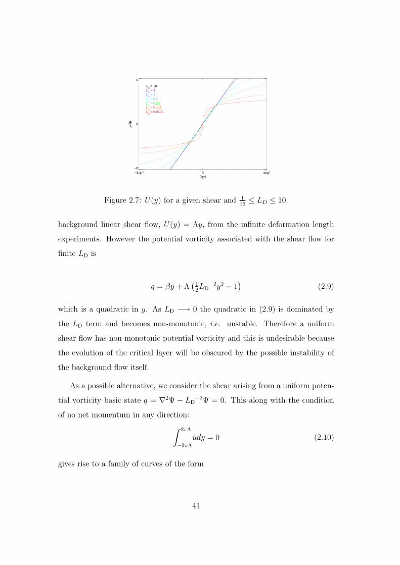
−4πµ2 0 4πµ2
U(y)
−π
0
π
y/2µ
LD = 10
LD = 2
LD = 1
LD = 0.5
LD = 0.25
LD = 0.125
LD = 0.0625
Figure 2.7: U(y) for a given shear and 116
≤ LD ≤ 10.
background linear shear flow, U(y) = Λy, from the infinite deformation length
experiments. However the potential vorticity associated with the shear flow for
finite LD is
q = βy + Λ(
12LD
−2y2 − 1)
(2.9)
which is a quadratic in y. As LD −→ 0 the quadratic in (2.9) is dominated by
the LD term and becomes non-monotonic, i.e. unstable. Therefore a uniform
shear flow has non-monotonic potential vorticity and this is undesirable because
the evolution of the critical layer will be obscured by the possible instability of
the background flow itself.
As a possible alternative, we consider the shear arising from a uniform poten-
tial vorticity basic state q = ∇2Ψ − LD−2Ψ = 0. This along with the condition
of no net momentum in any direction:
∫ 2πΛ
−2πΛ
udy = 0 (2.10)
gives rise to a family of curves of the form
41

U(y) =A
LD
sinh
(
y
LD
)
(2.11)
where A is a constant. Subsequently we examined two different conditions to find
the constant A. The first condition was to define the shear at the center of the
channel (y = 0) to be the same as the shear profiles investigated in the infinite
deformation length experiments. This resulted in A = ΛLD2 where uy |y=0= Λ.
The other condition considered was that the velocity difference across the channel
was the same as in the LD−1 = 0 cases. This gave
A =Λ2πΛLD
sinh(2πΛLD
)(2.12)
where y = ±2πΛ represents the channel walls. However neither of these condi-
tions were suitable for our investigation. In the case of the first condition the
velocities at the channel walls were too large at small LD for the numerical cal-
culation due to the hyperbolic sine term in (2.11). For the second condition the
width of the critical layer equalled the width of the channel at small LD due to
the small velocities across the channel. This then caused uncertainties over the
effects of the boundaries on the evolution.
Ultimately we decided that the average shear over the width of the critical
layer should be comparable to the shear over the critical layer in the infinite
Rossby deformation length experiments. We defined a top hat weighting
g(y) =
12yc
if |y| < yc
0 otherwise.(2.13)
where yc = 25(2πΛ) denotes the edge of the critical layer (critical layer is 2
5of the
channel width), such that the average shear over the critical layer is equal to Λ
as follows
42
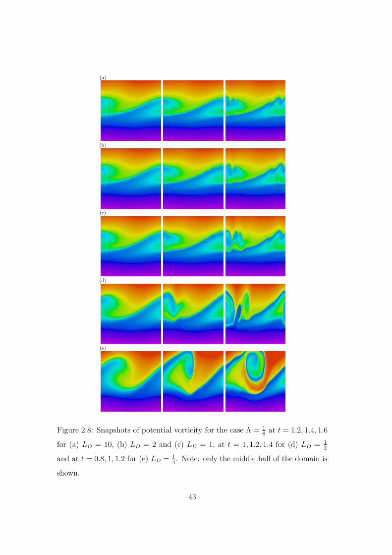
(a)
(b)
(c)
(d)
(e)
Figure 2.8: Snapshots of potential vorticity for the case Λ = 18
at t = 1.2, 1.4, 1.6
for (a) LD = 10, (b) LD = 2 and (c) LD = 1, at t = 1, 1.2, 1.4 for (d) LD = 12
and at t = 0.8, 1, 1.2 for (e) LD = 14. Note: only the middle half of the domain is
shown.
43

∫ l
−l
g(y)uydy = Λ (2.14)
∫ yc
−yc
uy1
2ycdy = Λ (2.15)
1
2yc(u(yc) − u(−yc)) = Λ (2.16)
The constant A in (2.11) is then defined from (2.14) to be
A =2ycLDΛ
[sinh( yc
LD) − sinh(−yc
LD)]
(2.17)
The background flow, U(y) (2.11), with A as defined above is shown in Fig-
ure 2.7 for a given shear and 116
≤ LD ≤ 10. The average shear in the critical
layer (i.e. between y = ±25(2πµ)) is equal to the shear Λ (= µ).
In the infinite Rossby deformation length experiments we defined a topo-
graphic streamfunction (ψtopo, ( 2.8)) that coincided with the perturbation stream-
function of the SWW solution (1978). In these experiments where LD is finite we
specify a topographic forcing qtopo such that ψtopo is the same as the infinite LD
cases. This yields
qtopo = ∇2ψtopo − LD−2ψtopo (2.18)
= −ǫµ cos(kx)
[
1 + LD−2
(
1 −cosh y
cosh(2πµ)
)]
(2.19)
It is important here that the streamline pattern of the background flow and the
topography is the same closed streamline pattern of the infinite LD experiments.
The reason for this is that the streamline pattern shows the relative importance
of u(0) and the topographic forcing and we want this to be constant across all Λ
and LD.
44

Figure 2.8 shows snapshots of the critical layer potential vorticity for Λ = 18
at
different times for different values of LD. Figure 2.8 demonstrates that when LD
is small (LD < 1) the width of the critical layer increases. This is an interesting
result because we have set the problem up so that as far as possible everything
is the same as the infinite LD cases (topographic forcing, average shear in the
critical layer region) and despite this we have found that the critical layer width
increases at small LD. The increase in critical layer width is due to the decrease in
LD and its consequent affect on the Rossby wave elasticity. When LD is relatively
large (Figure 2.8 (a), (b) and (c)) and we perturb the potential vorticity contours,
the contours resist the motion due to Rossby wave elasticity and are therefore
difficult to deform. In contrast at smaller LD (Figure 2.8 (d) and (e)) the Rossby
wave elasticity is weakened and hence there is less resistance to the deformation
of potential vorticity contours resulting in a wider critical layer. Note that the
increase in critical layer width is not due to a resonance with the topography (as
occurred in the infinite deformation length cases). Other experiments at smaller
LD showed further increases in the critical layer width indicating that this is a
trend (not resonance). Also the time evolution of the critical layers in these cases
does not show linear growth in the critical layer width.
2.4.2 Scaling of the Critical Layer Width
To estimate the growth of the critical layer width at small LD we adjust the
forcing. This adjusted forcing takes into account that the potential vorticity
contours are more deformable at small LD. We require the amplitude of the to-
pographic forcing in the critical layer to decrease as LD decreases. The amplitude
of the original topographic forcing was ǫµ where ǫ ≪ 1 (see (2.18)) and this is
adjusted to
45
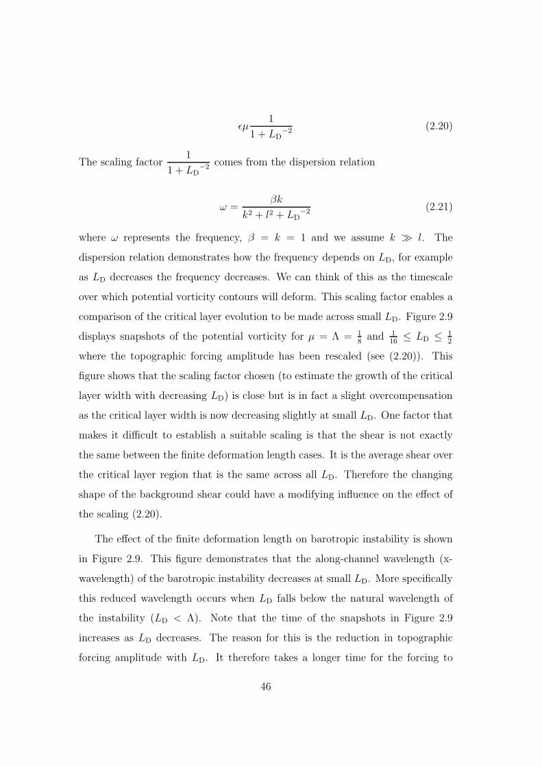
ǫµ1
1 + LD−2 (2.20)
The scaling factor1
1 + LD−2 comes from the dispersion relation
ω =βk
k2 + l2 + LD−2 (2.21)
where ω represents the frequency, β = k = 1 and we assume k ≫ l. The
dispersion relation demonstrates how the frequency depends on LD, for example
as LD decreases the frequency decreases. We can think of this as the timescale
over which potential vorticity contours will deform. This scaling factor enables a
comparison of the critical layer evolution to be made across small LD. Figure 2.9
displays snapshots of the potential vorticity for µ = Λ = 18
and 116
≤ LD ≤ 12
where the topographic forcing amplitude has been rescaled (see (2.20)). This
figure shows that the scaling factor chosen (to estimate the growth of the critical
layer width with decreasing LD) is close but is in fact a slight overcompensation
as the critical layer width is now decreasing slightly at small LD. One factor that
makes it difficult to establish a suitable scaling is that the shear is not exactly
the same between the finite deformation length cases. It is the average shear over
the critical layer region that is the same across all LD. Therefore the changing
shape of the background shear could have a modifying influence on the effect of
the scaling (2.20).
The effect of the finite deformation length on barotropic instability is shown
in Figure 2.9. This figure demonstrates that the along-channel wavelength (x-
wavelength) of the barotropic instability decreases at small LD. More specifically
this reduced wavelength occurs when LD falls below the natural wavelength of
the instability (LD < Λ). Note that the time of the snapshots in Figure 2.9
increases as LD decreases. The reason for this is the reduction in topographic
forcing amplitude with LD. It therefore takes a longer time for the forcing to
46

(a) (b) (c) (d)
Figure 2.9: Snapshots of potential vorticity after rescaling the topography by
(1+LD−2)−1 for Λ = 1
8and (a) LD = 1
2, (b) LD = 1
4, (c) LD = 1
8and (d) LD = 1
16
(t = 1.8, 2.2, 4, 10 respectively). Note: only the middle third of the domain is
shown.
have an effect.
2.5 Conclusions
In this chapter we have investigated the evolution of barotropic instability
within a critical layer. Our work differs from that of SWW (1978) and Haynes
(1989) in that we force the streamfunction in the critical layer directly (rather
than force laterally) using the SWW solution as a model for the critical layer.
Another difference is that our numerical model is a dimensional model rather
than a non-dimensional model used in Haynes (1989).
We examined the effect of the shear across the critical layer on the critical
layer evolution, and more specifically on the development of barotropic instability
in the critical layer. We found (consistent with Haynes (1989)) that barotropic
instability occurred when the shear was suitably small, Λ ≤ 0.3. As the shear
across the critical layer decreased the along-channel wavelength of the instability
decreased (wavenumber increased). The mixing efficiency of the critical layer
increased due to barotropic instability. We also found that barotropic instability
47

enhances mixing in the critical layer at early times when the shear is small.
However this enhancement is much smaller than the enhancement of mixing due
to the resonant growth of the critical layer around Λ = 12.
In an extension to previous work we carried out a systematic investigation of
the critical layer evolution at finite Rossby deformation length. We set up this
investigation so that as far as possible everything was the same as the infinite
Rossby deformation length investigation, i.e. topographic forcing and average
shear in the critical layer region (same closed streamline pattern). We found
that regardless of this the critical layer width increased at small LD. This was
due to the effect of LD on the Rossby wave elasticity. We therefore chose to
estimate the growth of the critical layer width with decreasing LD. We adjusted
the topographic forcing amplitude using a scaling factor from the Rossby wave
dispersion relation. The scaling factor chosen was close but overcompensated for
the increase in the critical layer width. The scaling factor allowed a study of the
effect of decreasing LD on the barotropic instability. We discovered that at small
LD, LD less than the natural wavelength of the instability, the wavelength of the
instability reduces.
48
Chapter 3
The Influence of Stratospheric
Potential Vorticity on Baroclinic
Instability
3.1 Introduction
Wavebreaking in the stratosphere drives the Brewer-Dobson circulation and
affects the mixing and transport of chemicals out of the tropical pipe (see chapter
5 for more details). In this chapter we discuss how this stratospheric wavebreaking
affects the troposphere and mixing at the tropopause and the Earth’s surface.
In recent years there has been much interest in the idea of dynamical cou-
pling between the stratosphere and the troposphere. It is widely known that wave
motions in the troposphere affect the stratospheric circulation, for example, plan-
etary waves which propagate up into the stratosphere and lead to stratospheric
* This chapter is based on: Smy, L. A. and Scott, R. K. 2009. The influence of stratospheric
potential vorticity on baroclinic instability. Q. J. R. Meteorol. Soc., 135, 1673-1683
49
sudden warmings. However recent observations now suggest that the stratosphere
may have an important influence on tropospheric weather and climate.
Observations of correlations between zonally symmetric anomalies of zonal
wind and geopotential height in the stratosphere and troposphere (e.g. Kodera
et al., 1990; Thompson & Wallace, 1998, 2000; Baldwin & Dunkerton, 1999)
have prompted this recent research into the dynamical coupling between these
two regions of the atmosphere. These correlations are time-lagged and show
tropospheric anomalies that persist on sub-seasonal timescales, longer than the
corresponding stratospheric anomalies. Consequently, it has been suggested that
the stratosphere may have a dynamical influence on the tropospheric circulation,
even to the extent that medium-range weather forecasts might be improved by
improving the representation of the stratosphere in forecast models (e.g. Scaife
& Knight, 2008).
Dynamical links between the stratosphere and troposphere have been sug-
gested to exist on both sub-seasonal and longer, inter-annual timescales. In the
latter case, for example, the stratosphere has been shown to influence tropo-
spheric circulation patterns in comprehensive general circulation models. Hart-
mann et al. (2000) investigated stratospheric ozone depletion as a possible cause
for the trends observed, since the 1970’s, in the stratospheric and tropospheric
annular modes. The effect of stratospheric ozone on solar cycle irradiance and
its resulting affect on climate change is examined by Shindell et al. (1999, 2001).
This influence of the stratosphere on the troposphere has also been shown in sim-
plified primitive equation models (Polvani & Kushner, 2002; Kushner & Polvani,
2004), where thermal perturbations in the stratosphere were found to signifi-
cantly affect the tropospheric circulation. This indicates the possible sensitivity
of the tropospheric circulation to the details of the stratospheric evolution. The
stratosphere is now widely believed to play an important role in climate variabil-
ity (e.g. WMO, 2007), although the dynamical processes involved are not well
50
understood.
On shorter timescales, on the other hand, the strong lag-correlations between
the strength of the winter stratospheric polar vortex and sea-level pressure dis-
tribution (Baldwin & Dunkerton, 1999, 2001; Thompson et al., 2002; Charlton
et al., 2003) again point to a dynamical coupling that remains, however, far from
well-understood. While descending zonal wind anomalies within the stratosphere
can be explained in terms of descending critical layers (Matsuno, 1971) , the per-
sistence of tropospheric anomalies on longer timescales requires consideration of
additional dynamical processes. For example, Song & Robinson (2004) have sug-
gested that stratospheric sudden warmings might couple with the troposphere
through an eddy-feedback mechanism. Another recent study by Thompson et al.
(2006) suggested, on the other hand, that the purely balanced response of the
troposphere to changes in stratospheric wave drag and thermal heating may be
sufficient to explain longer tropospheric correlation timescales.
The main driver of surface weather systems in the troposphere is baroclinic
instability. A dynamical link between the stratosphere and troposphere involving
the modulation of baroclinic instability by stratospheric zonal wind anomalies has
also been considered recently (Wittman et al., 2004, 2007) . In simple baroclinic
lifecycle experiments using a general circulation model dynamical core, Wittman
et al. (2004) found that the strength of the stratospheric zonal winds had an
influence on the tropospheric evolution, both in terms of the synoptic scale de-
velopment and in zonal mean quantities, such as surface geopotential. Building
on this and earlier work by Muller (1991) that examined linear growth rates in a
one-dimensional Eady-type model, Wittman et al. (2007) further examined the
dependence of growth rates on stratospheric shear in a variety of simple and
more comprehensive models. In particular, they found that increasing the verti-
cal shear above the tropopause (a representation of a strong stratospheric vortex)
increased growth rates across a range of zonal wavenumbers.
51

In this chapter, we again investigate the dynamical link between stratospheric
anomalies and baroclinic instability, but here restrict attention to anomalies that
consist purely of a change to the stratospheric potential vorticity. This approach
is motivated by a recognition of potential vorticity as the principle dynamical
quantity governing the slow, balanced motion of the stratosphere. A strong polar
vortex is an approximately zonally symmetric distribution of high potential vor-
ticity, while a weak polar vortex may be due either to a distribution of low poten-
tial vorticity, or, alternatively, to a zonally asymmetric distribution of potential
vorticity. The latter scenario is what is typically observed during major strato-
spheric sudden warmings, when strong planetary wave breaking redistributes the
stratospheric potential vorticity, either through a strong displacement of the vor-
tex (in the case of a wave-1 warming) or through a vortex split (in the case of
a wave-2 warming; e.g. Charlton & Polvani, 2007). The location of the polar
vortex affects the horizontal shear around the tropopause and at the surface (see
figure 3.1). Therefore we expect changes to the location of the polar vortex to
change the critical layer dynamics at the tropopause and at the surface. The ap-
proach adopted here allows us to examine in detail how such a redistribution of
the stratospheric potential vorticity may effect the tropospheric evolution. Note
also that we are interested in resultant changes to the nonlinear tropospheric
evolution during the course of a baroclinic lifecycle rather than in changes to
the tropospheric circulation resulting from an instantaneous potential vorticity
inversion. The effects of zonal mean perturbations to the stratospheric potential
vorticity on the tropospheric circulation as a direct result of potential vorticity
inversion were considered by Ambaum & Hoskins (2002); Black (2002), but not
their influence on baroclinic instability.
For simplicity, and to avoid the difficulties involved in balancing an asym-
metric potential vorticity distribution, we use a quasigeostrophic model on an
f -plane. The model configuration is described fully in section 3.2. Baroclinic
52

instability is arranged in the troposphere through an Eady-type distribution of
potential temperature at the surface and tropopause. The case in which the
stratospheric potential vorticity is exactly zero is treated as a control (discussed
in section 3.3.1). Following this we consider the effect on the instability of zonally
symmetric perturbations to the stratospheric potential vorticity (as a represen-
tation of a strong vortex, section 3.3.2) and asymmetric perturbations (as a rep-
resentation of the vortex following a sudden warming, section 3.3.3). Finally, we
briefly consider the sensitivity of our results to details of the tropospheric mean
state (section 3.3.4)
3.2 Model description
The numerical model used is the contour advective semi-Lagrangian (CASL)
model developed originally by Dritschel & Ambaum (1997) and extended to
cylindrical geometry by Macaskill et al. (2003) which solves the quasigeostrophic
equations on an f plane in a cylindrical domain in uniform rotation about the
central axis. A quasigeostrophic framework is used since it captures the domi-
nant balance in the atmosphere, namely large-scale low frequency motions and
filters out small scales, for example gravity waves. In the model contours of
constant quasigeostrophic potential vorticity are advected layerwise by the asso-
ciated geostrophic velocity field. One advantage of this model is that it allows
easy initialisation of both zonal and non-zonal potential vorticity anomalies and
a relatively straightforward interpretation of dynamical processes.
In cylindrical coordinates (r, θ, z) the equations take the form
Dq
Dt=∂q
∂t+ u · ∇q = 0 (3.1)
q =1
r
∂
∂r
(
r∂ψ
∂r
)
+1
r2
∂2ψ
∂θ2+
1
ρ0
∂
∂z
(
ρ0f 2
0
N2
∂ψ
∂z
)
(3.2)
53

u =
(
−1
r
∂ψ
∂θ,∂ψ
∂r
)
(3.3)
together with an isothermal lower boundary condition ψz = 0 at z = 0.
Here q is the (anomalous) quasigeostrophic potential vorticity, ψ is the geostrophic
streamfunction, and u = (u, v) is the horizontal geostrophic velocity. The phys-
ical parameters are the background density ρ0 = ρs exp(−z/H), where H is
a vertical scale height and ρs is a surface reference density, the “midlatitude”
Coriolis parameter f0 = 2Ω sin 45, where Ω = 2π day−1 is the (planetary) rota-
tion rate, and the constant buoyancy frequency N . Numerically, we have chosen
N ≈ 0.018 s−1 and H ≈ 8800m as being representative of the troposphere, giving
a Rossby deformation radius LR = NH/f0 of approximately 1525 km.
We use an Eady type approximation in which the interior tropospheric poten-
tial vorticity is uniform and potential vorticity anomalies are concentrated in thin
layers near the surface and the tropopause. The standard Eady model has a basic
state consisting of a uniform vertical shear U = Λz corresponding to a uniform
latitudinal potential temperature gradient Θ = −Λy, together with lower and
upper boundary conditions ψz = θ at z = 0 and z = H . Following Bretherton
(1966) this can be recast in terms of the evolution of upper and lower potential
vorticity sheets with basic state
Q = Θδ(z) − Θδ(z −H) (3.4)
together with isothermal boundary conditions at z = 0 and z = H . As discussed
in Juckes (1994), replacing the upper boundary at z = H with a tropopause
separating regions with static stability Ntrop (tropospheric) and Nstrat (strato-
spheric) leads to the same expression but with a factor proportional to (Ntrop −
Nstrat)/NtropNstrat multiplying the sheet at z = H (see Eq. 3.11 in Juckes, 1994).
Since here we are interested in the dynamics of a jet localised in latitude, we gen-
eralise the Eady basic state to a nonuniform function of latitude. This motivates
54
the following definition for the total basic state potential vorticity
q = θs(r)δ(z) − θt(r)δ(z −H) + qstrat (3.5)
with θs and θt corresponding to Θ in (3.4) and where qstrat is a basic state strato-
spheric potential vorticity to be specified below.
The jump in N2 in the atmosphere will lead to tropopause dynamics (Juckes,
1994) in which potential vorticity is essentially a delta function at the tropopause.
Surface temperature, θs, can also be considered as a sheet distribution of potential
vorticity (see Hoskins et al., 1985). Sheet dynamics are similar to two dimensional
dynamics at large scales (L >> LR), however the equations of a sheet are more
local and therefore more small scales (L << LR) develop than in two dimensions.
The initial surface and tropopause potential temperature distributions are
specified by a simple latitudinal profile of the form
θs,t(r) = ∆θs,t tanh((rj − r)/w) (3.6)
of width 2w = LR and centred at rj = 4LR (approximately 30 latitude). A
hyperbolic tangent profile was chosen to represent the potential temperature jump
as a compromise between q = H(y), where H is the Heaviside function (H(y) = 0
if y < 0 and H(y) = 1 if y > 0), and q = βy. The former is singular in this
model while the latter tends not to be observed since wave breaking and mixing
steepen potential vorticity gradients. Furthermore we can vary the width of the
profile in (3.6) with a single parameter, w. In practice we want a width of the
order of a Rossby deformation radius. This is similar to the size of typical eddies
developing in a baroclinic flow and therefore the zonal average potential vorticity
is smooth over a distance of a Rossby deformation radius. The choice 2w = LR
is again a compromise between extremes. The sensitivity of our results to this
parameter (w) is described briefly in section 3.3.4.
Analogously to (3.4), ∆θs,t correspond to the pole–equator potential temper-
ature differences at the surface and tropopause, with ∆θs,∆θt < 0. The values
55

of ∆θs and ∆θt were chosen to give our model realistic shear in the troposphere
( 50ms−1). If there is a single jump in potential temperature then the jet as-
sociated with that jump depends linearly on the potential temperature jump
(two-dimensional barotropic case). It therefore seems reasonable that u increases
linearly with the total jump in potential temperature,
u = α(−∆θt + σ∆θs) (3.7)
where α and σ are constants. Note that this is an approximate equation. We
deduced the velocity u at the tropospheric jet (ut) and at the surface (us) by
setting ∆θt = 0 and estimating the velocity (either ut or us) from the initial
wind plots produced and then repeating this but with ∆θs = 0. We then set
us = 0 and ∆u = ut− us = 50, consistent with NCEP Statistical and Climatolog-
ical Analyses (http://acdb-ext.gsfc.nasa.gov/Data services/met/mzm.html) and
solved for ∆θs and ∆θt. Choosing values ∆θs = −0.2 and ∆θt = −0.6 gives a
basic state comprising a subtropical jet with a maximum u of about 35ms−1 and
a vertical shear amounting to a difference of about 50ms−1 between the surface
and tropopause, as shown in Figure 3.1(a).
The distribution of potential vorticity in the winter stratosphere is dominated
almost entirely by the polar vortex, and may be approximated most simply as
a region of high potential vorticity over the pole and low potential vorticity in
midlatitudes. In our model we therefore define qstrat by
qstrat(r, z) =
∆Q if r < rv, z ≥ 1.5H
0 otherwise
(3.8)
where rv is the vortex radius at a given height and ∆Q is the jump in potential
vorticity at the vortex edge. Here the lowermost vortex is situated at a distance
of 0.5H above the tropopause, as a crude representation of the weaker “subvortex
region” and to reduce the direct effect of the stratospheric potential vorticity on
56

0
1
2
3
0 2 4 6radius
heig
ht
0 2 4 6radius
0 2 4 6radius
0 2 4 6radius
(a) (b) (c) (d)
Figure 3.1: Initial zonal wind profiles of the four main cases (a) zero stratospheric
potential vorticity (the control case), (b) zonally symmetric polar vortex, (c)
asymmetric polar vortex (displaced) and (d) asymmetric polar vortex (split).
The stratospheric potential vorticity jump in (b-d) is ∆Q = 0.4f0. The contour
interval is 5ms−1.
(a) (b) (c) (d)
Figure 3.2: Perspective view of the potential vorticity contours in the four main
cases: (a-d) as in Figure 3.1.
57
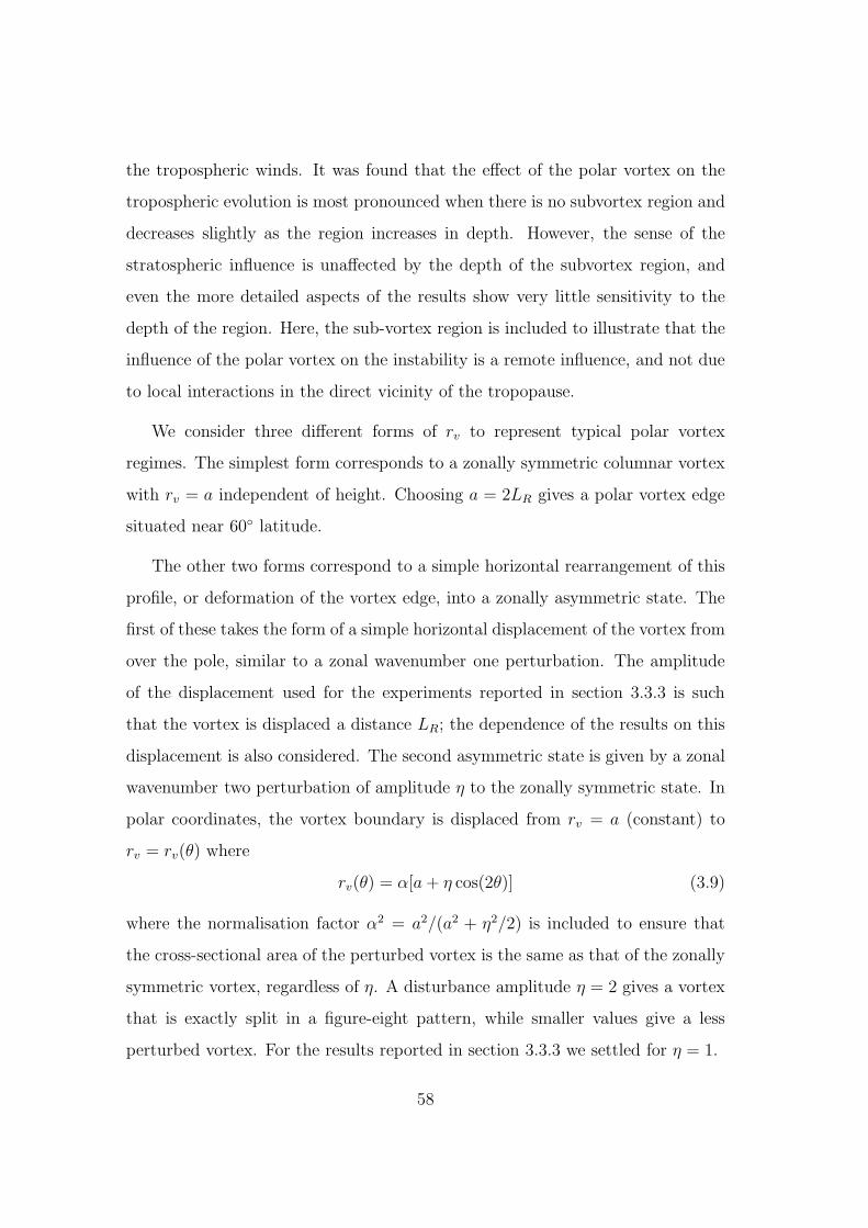
the tropospheric winds. It was found that the effect of the polar vortex on the
tropospheric evolution is most pronounced when there is no subvortex region and
decreases slightly as the region increases in depth. However, the sense of the
stratospheric influence is unaffected by the depth of the subvortex region, and
even the more detailed aspects of the results show very little sensitivity to the
depth of the region. Here, the sub-vortex region is included to illustrate that the
influence of the polar vortex on the instability is a remote influence, and not due
to local interactions in the direct vicinity of the tropopause.
We consider three different forms of rv to represent typical polar vortex
regimes. The simplest form corresponds to a zonally symmetric columnar vortex
with rv = a independent of height. Choosing a = 2LR gives a polar vortex edge
situated near 60 latitude.
The other two forms correspond to a simple horizontal rearrangement of this
profile, or deformation of the vortex edge, into a zonally asymmetric state. The
first of these takes the form of a simple horizontal displacement of the vortex from
over the pole, similar to a zonal wavenumber one perturbation. The amplitude
of the displacement used for the experiments reported in section 3.3.3 is such
that the vortex is displaced a distance LR; the dependence of the results on this
displacement is also considered. The second asymmetric state is given by a zonal
wavenumber two perturbation of amplitude η to the zonally symmetric state. In
polar coordinates, the vortex boundary is displaced from rv = a (constant) to
rv = rv(θ) where
rv(θ) = α[a+ η cos(2θ)] (3.9)
where the normalisation factor α2 = a2/(a2 + η2/2) is included to ensure that
the cross-sectional area of the perturbed vortex is the same as that of the zonally
symmetric vortex, regardless of η. A disturbance amplitude η = 2 gives a vortex
that is exactly split in a figure-eight pattern, while smaller values give a less
perturbed vortex. For the results reported in section 3.3.3 we settled for η = 1.
58

The complete tropospheric and stratospheric vorticity distributions are shown
in a perspective view in Figure 3.2. Note that we have added a weak (maximum
displacement of 0.1LD) zonal wavenumber 6 perturbation to the surface and
tropopause potential temperature fields to seed the baroclinic instability. This is
the fastest growing mode, and a single wavenumber perturbation was chosen to
allow direct comparison of surface potential temperature fields among different
cases during the nonlinear stages of the evolution. The control case, with qstrat = 0
is shown in Figure 3.2(a) and the cases with stratospheric perturbation—zonally
symmetric, displaced vortex, and split vortex—in Figure 3.2(b-d), respectively.
The corresponding initial zonal velocity profiles for each case are shown in Fig-
ure 3.1
The model equations are discretized using 80 layers in the vertical between
z = 0 and z = 3H . This gives a vertical domain extending from the ground to
approximately the middle stratosphere. In this problem, the upper stratospheric
potential vorticity has practically no impact on details of the tropospheric winds
and the evolution of the baroclinic lifecycle, so this truncation seems justified. In
the horizontal directions, the streamfunction and velocity fields are calculated on
a stretched grid of 128 radial and 264 azimuthal points, although the potential
vorticity itself is first interpolated onto a grid four times finer for more accurate
inversion. The lateral boundary is located at a distance of 8LR from the pole and
has been verified to have practically no effect on the tropospheric evolution.
Finally, a few words are needed concerning the issue of numerical convergence.
In the Eady model, the surface and tropopause dynamics exhibit a logarithmic
singularity in the tangential velocity field as potential temperature fronts develop
(Juckes, 1994). Further, steep potential temperature gradients are a natural fea-
ture of the nonlinear evolution during the instability. The logarithmic singularity
is here regularized by the fact that the vertical discretization is finite, but in-
creasing vertical resolution results in increasingly energetic flow at the smallest
59

horizontal scales. It was found by successively doubling both horizontal and ver-
tical resolution together that, although the smallest-scale features of the model
continue to exhibit differences at the highest resolution performed, large and
synoptic-scale features are essentially convergent. Further, bulk quantities like
the eddy kinetic energy are convergent below the resolution used for the main
experiments reported below.
3.3 Results
3.3.1 Control
We first briefly describe the control case in which the stratospheric potential
vorticity is exactly zero. The initial zonal wind profile for this case is shown in
Figure 3.1(a) and, as described above, comprises a baroclinically unstable sub-
tropical jet with peak wind speed of approximately 35ms−1 and a vertical shear
amounting to a difference of about 50ms−1 between the surface and tropopause.
The growth of the instability is such that significant nonlinearity develops
by around days 6–8 of the evolution, with eddy kinetic energy peaking near day
10 and then decreasing again in a decay stage, the classic baroclinic lifecycle
paradigm. The synoptic surface potential temperature distribution for the con-
trol case at days 10, 12 and 14 of the lifecycle evolution is shown in Figure 3.3(a-c).
Significant nonlinearity has developed by day 10 with the usual wave breaking,
irreversible mixing of potential vorticity, and intensification of potential temper-
ature gradients. Because of the simplicity of our model only a very qualitative
comparison of this evolution with that observed in more sophisticated models is
possible. However, the evolution can be regarded as broadly similar to the LC1
lifecycle of Thorncroft et al. (1993) with predominantly anticyclonic equatorward
wave breaking during the saturation phase. Examination of the zonal mean zonal
60

(a) (b) (c)
(d) (e) (f)
Figure 3.3: Surface potential temperature at days 10, 12 and 14: (a-c) the control
case ∆Q = 0; (d-f) with a zonally symmetric stratospheric anomally of ∆Q =
0.4f0.
61

velocity and wave fluxes (not shown) indicate a transfer of energy into a deeper
barotropic jet and an upward wave flux from the surface to the tropopause.
3.3.2 Zonally Symmetric Perturbation
To examine the effect of stratospheric potential vorticity on the tropospheric
evolution we next consider cases with nonzero qstrat. We first consider the case of
a zonally symmetric perturbation to the stratospheric potential vorticity. More
realistic perturbations will follow in section 3.3.3, but we note for now that a
zonally symmetric perturbation can be regarded as a crude representation of
a strong polar vortex, and can therefore be contrasted with the control case
discussed above (which can be regarded as an extreme example of a weak vortex).
Our comparison here is similar to the situation considered by Wittman et al.
(2004), who restricted attention to purely zonally symmetric initial conditions,
with or without a stratospheric polar vortex.
The zonally symmetric perturbation to the stratospheric potential vorticity is
defined by (3.8) with rv = a = 2LR. Here we focus on the case ∆Q = 0.4f0, which
gives rise to a relatively strong polar vortex (in terms of u near the vortex edge),
but the intermediate case of ∆Q = 0.2f0 is also discussed briefly. As can be seen in
Figure 3.1, the addition of the polar vortex in the stratosphere has a direct effect
on the initial state tropospheric zonal wind due to potential vorticity inversion.
Note, however, that although the tropospheric jet has increased to a maximum of
45ms−1 (compared with 35ms−1 in the control), the vertical shear between the
surface and tropopause is largely unchanged. In contrast, the addition of the polar
vortex results in a more significant change to the horizontal shear throughout the
troposphere, which has a subsequent effect on the tropospheric evolution.
Figure 3.3(d-f) shows the synoptic surface potential temperature evolution
for the zonally symmetric perturbation with ∆Q = 0.4f0 at days 10, 12 and 14.
62

0
1
2
3
4
0 4 8 12 16
t (days)
EKE *104
Figure 3.4: Eddy kinetic energy as a function of time for the cases with a zonally
symmetic polar vortex with ∆Q = 0 (bold solid), ∆Q = 0.2f0 (dashed), and
∆Q = 0.4f0 (thin solid).
Again, the baroclinic instability results in wave breaking and irreversible mix-
ing across the jet. However, in the perturbed case increased horizontal shear
throughout the troposphere results in a change in the critical dynamics and an
eddy growth that is now more confined in latitude than before. This interpreta-
tion is consistent with the results of Thorncroft et al. (1993) where the addition of
barotropic shear to the initial mean zonal flow of an LC1 lifecycle resulted in sig-
nificantly different nonlinear dynamics (the LC2 lifecycle). While interpretation
of the evolution shown in Figure 3.3 in terms of LC1 and LC2 lifecycles is diffi-
cult owing to the simplicity of our model, there are nevertheless clear differences
between the two cases. For example, both the strong equatorward wave breaking
of the control case and the weaker, poleward wavebreaking are attenuated in the
case with ∆Q = 0.4f0. At later times, days 12–14, the poleward breaking in
the control case results in strong transport of low-latitude air into high latitudes,
which is much weaker in the perturbation case.
63
To quantify the change in eddy growth with changes to the stratospheric po-
tential vorticity we show in Figure 3.4 the eddy kinetic energy as a function of
time for the case of exactly zero stratospheric potential vorticity (the control, for
which ∆Q = 0) and two cases with increasing strength of stratospheric potential
vortex anomalies, ∆Q = 0.2f0 and ∆Q = 0.4f0. At early times there is a decrease
in the growth rate of eddy kinetic energy with increasing ∆Q, and, consequently,
a reduction in the maximum value obtained around day 10. At first sight, this
dependence might appear contrary to the results of Wittman et al. (2007) who
found using a primitive equation model that the growth rate of eddy kinetic
energy increased monotonically (at wavenumbers less than 7) with increasing
vertical shear in the stratosphere, their proxy for the polar vortex. In fact, the
two sets of results appear to be consistent when we take into account the details
of the changes to the initial shear caused by the stratospheric perturbations in
each case. In Wittman et al., the addition of vertical shear in the stratosphere
appears to enhance the eddy growth rate in a similar way as increasing the ver-
tical shear in the troposphere in the traditional Eady model. In our model, on
the other hand, the addition of the stratospheric potential vorticity anomally has
practically no effect on the vertical shear in the troposphere or anywhere near the
subtropical jet (Figure 3.1(a) and (b)). As discussed above, however, it does in-
crease the horizontal shear throughout the troposphere with a resultant change in
the character of the lifecycle, consistent with Thorncroft et al. (1993). Of course,
other differences between the two modelling frameworks (e.g. cylindrical versus
spherical geometry, quasigeostrophic versus primitive equations, latitudinal off-
set between the polar vortex and the subtropical jet) may also alter details of
the evolution. However, the dependence of the growth rates on the tropospheric
shear would appear to be consistent.
Another useful measure of eddy growth, particularly suited to the contour
64

representation used here, is the wave activity A defined as
A(z, t) =1
4ρ0(z)
∑
k
qk
∮
Γk(z)
(
r2 − r2e
)2dθ (3.10)
where the sum is over all contours Γk in a given vertical level, where re is the
radius of the undisturbed circular contour enclosing the same area as Γk, and
where qk is the vorticity jump on the kth contour. This is a nonlinear pseudo-
momentum based wave activity, second order in disturbance amplitude, satisfying
an exact conservation relation (see Dritschel, 1988; Dritschel & Saravanan, 1994,
for more details). The evolution of total wave activity contained in the surface and
tropopause potential temperature fields is shown in Figure 3.5 for the three cases
∆Q = 0, 0.2f0, 0.4f0. Like the eddy kinetic energy, the wave activity increases
due to the instability, and again with weaker growth at higher values of ∆Q. At
late times the difference between the cases is even more marked, with continued
increase in the wave activity in the case ∆Q = 0 but not in the other cases.
We note incidentally that these differences in the tropospheric wave activity are
entirely due to the evolution of the basic instability: the amount of wave activity
“leaking” from the troposphere into the polar vortex is negligible, with values of
the stratospheric wave activity remaining around five orders of magnitude less
than tropospheric values throughout the evolution.
As in Wittman et al. (2004) it is also possible to consider the surface geopo-
tential height difference as a crude measure of the extent to which the instability
projects onto the Arctic Oscillation. Figure 3.6 shows the difference between the
surface geopotential height anomaly at day 12 and day 0. The magnitude of the
dipole structure resulting from the instability becomes weaker for larger values of
∆Q, consistent with the reduction of eddy growth rates discussed above. Again
the different dependence on ∆Q from the dependence found in Wittman et al.
(2004) can be understood in terms of changes to the tropospheric shear induced
by the stratospheric perturbation.
65

0
1
2
3
4
0 4 8 12 16
t (days)
wave activity
Figure 3.5: Combined surface and tropopause wave activity as a function of time
for the cases ∆Q = 0 (bold solid), ∆Q = 0.2f0 (dashed), and ∆Q = 0.4f0 (thin
solid). Values have been normalized by the initial angular impulse of the case
∆Q = 0.
Finally we examine the effect of the stratospheric perturbation on the growth
rate of other wavenumber disturbances to the surface and tropopause basic state.
Here we consider the difference between the two cases ∆Q = 0 and ∆Q = 0.4f0
and calculate the linear growth rates of different wavenumbers by integrating
the model at early times only. One reason for doing so is to verify that the
addition of a polar vortex indeed reduces the growth rate at all wavenumbers
rather than simply shifting the wavenumber of the fastest growing mode. As
seen in Figure 3.7 this is indeed the case, with a modest reduction in growth rate
across all wavenumbers.
3.3.3 Asymmetric Perturbations
We now consider the effect of asymmetric perturbations to the stratospheric
potential vorticity on the tropospheric evolution. Again, these perturbations are
66

-5
-4
-3
-2
-1
0
1
2
3
4
5
0 2 4 6 8radius
surface geopotentialdifference
Figure 3.6: Difference between the surface geopotential at day 12 and day 0 for
the cases ∆Q = 0 (bold solid), ∆Q = 0.2f0 (dashed), and ∆Q = 0.4f0 (thin
solid).
0
0.1
0.2
0.3
0.4
0.5
0.6
0.7
0.8
0.9
1.0
0 1 2 3 4 5 6 7 8
wavenumber
growth rate
Figure 3.7: The linear growth rate of eddy kinetic energy with different initial
wavenumber perturbations in the troposphere: ’s correspond to the control
case, ∆Q = 0, and 2’s correspond to a zonally symmetric stratospheric polar
vortex with ∆Q = 0.4f0.
67
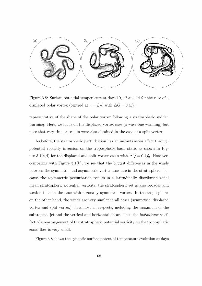
(a) (b) (c)
Figure 3.8: Surface potential temperature at days 10, 12 and 14 for the case of a
displaced polar vortex (centred at r = LR) with ∆Q = 0.4f0.
representative of the shape of the polar vortex following a stratospheric sudden
warming. Here, we focus on the displaced vortex case (a wave-one warming) but
note that very similar results were also obtained in the case of a split vortex.
As before, the stratospheric perturbation has an instantaneous effect through
potential vorticity inversion on the tropospheric basic state, as shown in Fig-
ure 3.1(c,d) for the displaced and split vortex cases with ∆Q = 0.4f0. However,
comparing with Figure 3.1(b), we see that the biggest differences in the winds
between the symmetric and asymmetric vortex cases are in the stratosphere: be-
cause the asymmetric perturbation results in a latitudinally distributed zonal
mean stratospheric potential vorticity, the stratospheric jet is also broader and
weaker than in the case with a zonally symmetric vortex. In the troposphere,
on the other hand, the winds are very similar in all cases (symmetric, displaced
vortex and split vortex), in almost all respects, including the maximum of the
subtropical jet and the vertical and horizontal shear. Thus the instantaneous ef-
fect of a rearrangement of the stratospheric potential vorticity on the tropospheric
zonal flow is very small.
Figure 3.8 shows the synoptic surface potential temperature evolution at days
68
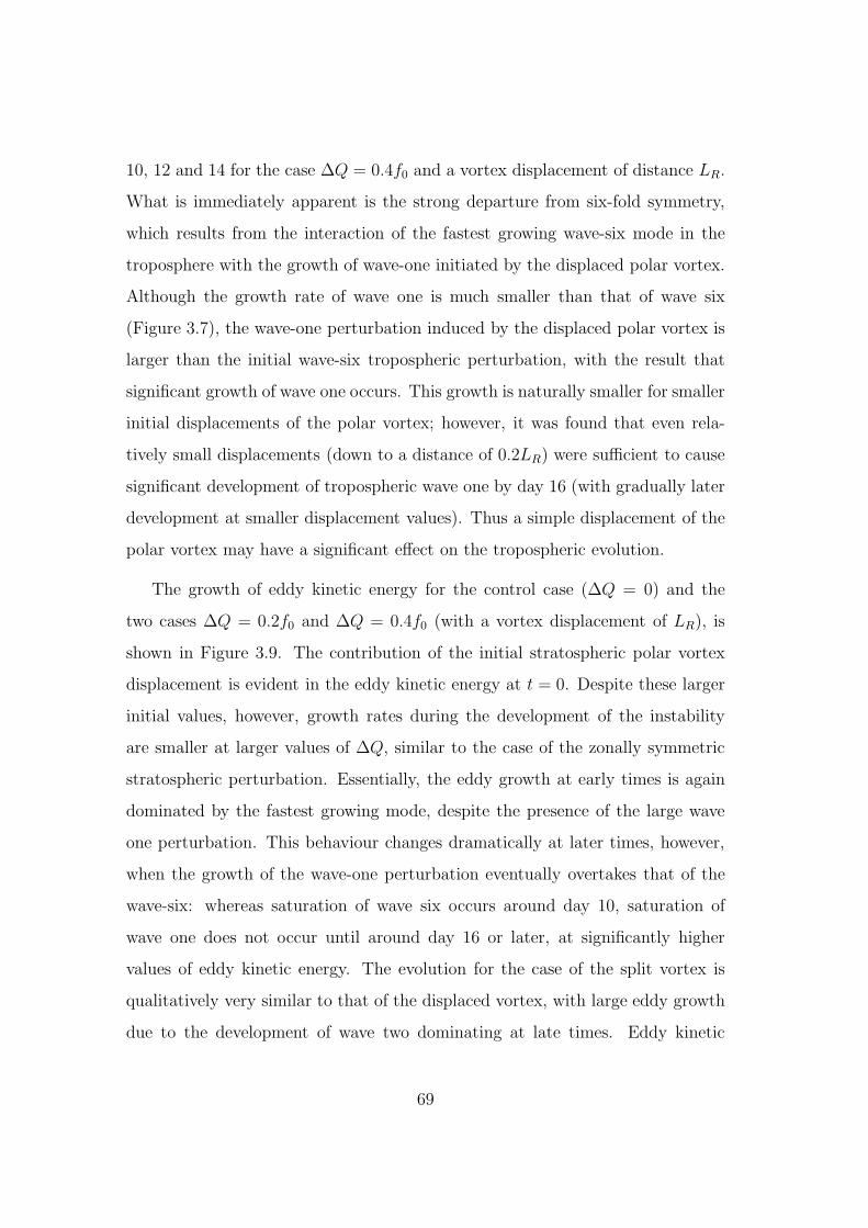
10, 12 and 14 for the case ∆Q = 0.4f0 and a vortex displacement of distance LR.
What is immediately apparent is the strong departure from six-fold symmetry,
which results from the interaction of the fastest growing wave-six mode in the
troposphere with the growth of wave-one initiated by the displaced polar vortex.
Although the growth rate of wave one is much smaller than that of wave six
(Figure 3.7), the wave-one perturbation induced by the displaced polar vortex is
larger than the initial wave-six tropospheric perturbation, with the result that
significant growth of wave one occurs. This growth is naturally smaller for smaller
initial displacements of the polar vortex; however, it was found that even rela-
tively small displacements (down to a distance of 0.2LR) were sufficient to cause
significant development of tropospheric wave one by day 16 (with gradually later
development at smaller displacement values). Thus a simple displacement of the
polar vortex may have a significant effect on the tropospheric evolution.
The growth of eddy kinetic energy for the control case (∆Q = 0) and the
two cases ∆Q = 0.2f0 and ∆Q = 0.4f0 (with a vortex displacement of LR), is
shown in Figure 3.9. The contribution of the initial stratospheric polar vortex
displacement is evident in the eddy kinetic energy at t = 0. Despite these larger
initial values, however, growth rates during the development of the instability
are smaller at larger values of ∆Q, similar to the case of the zonally symmetric
stratospheric perturbation. Essentially, the eddy growth at early times is again
dominated by the fastest growing mode, despite the presence of the large wave
one perturbation. This behaviour changes dramatically at later times, however,
when the growth of the wave-one perturbation eventually overtakes that of the
wave-six: whereas saturation of wave six occurs around day 10, saturation of
wave one does not occur until around day 16 or later, at significantly higher
values of eddy kinetic energy. The evolution for the case of the split vortex is
qualitatively very similar to that of the displaced vortex, with large eddy growth
due to the development of wave two dominating at late times. Eddy kinetic
69

0
1
2
3
4
0 4 8 12 16
t (days)
EKE *104
Figure 3.9: Eddy kinetic energy as a function of time for a displaced polar vortex
(centred at r = LR) with ∆Q = 0 (bold solid, same as the control case), ∆Q =
0.2f0 (dashed), and ∆Q = 0.4f0 (thin solid).
energy plots for this case are similar to those shown in Figure 3.9, while the
surface potential temperature fields show the late time development of wave four
due to the interaction of the wave six and wave two initial perturbations.
Instead of comparing the tropospheric evolution at different ∆Q, it is perhaps
more instructive to consider the differences between the zonally symmetric and
displaced polar vortex cases, both with ∆Q = 0.4f0, the potential vorticity in the
displaced vortex case being simply a redistribution of that in the symmetric case.
The surface potential temperature fields (compare Figure 3.3(d-f) and Figure 3.8)
are significantly different between the two cases already at day 10, but still more so
at late times, when much more vigorous mixing is found across a wider latitudinal
region in the displaced vortex case. Similarly, the eddy kinetic energy shows
significant differences at late times (compare thin solid lines in Figure 3.4 and
Figure 3.9), although growth rates at early times are similar.
The more vigorous mixing across latitude has an influence on the zonal mean
70

-5
-4
-3
-2
-1
0
1
2
3
4
5
0 2 4 6 8radius
surface geopotentialdifference
Figure 3.10: Difference between the surface geopotential height at day 12 and
day 0 for the displaced polar vortex (centred at r = LR) with ∆Q = 0 (bold
solid), ∆Q = 0.2f0 (dashed), and ∆Q = 0.4f0 (thin solid).
surface geopotential height anomalies considered above. Figure 3.10 again shows
the difference between the surface geopotential height anomaly at day 12 and
day 0, for ∆Q = 0, 0.2f0, 0.4f0 but for the displaced vortex cases. As in the case
of the zonally symmetric vortex, large ∆Q again results in a less pronounced
dipolar structure in midlatitudes. Comparing the thin solid line in this figure
with that in Figure 3.6 indicates that the redistribution of potential vorticity
in the stratosphere has also had an effect on the resulting surface geopotential
height following the baroclinic development.
Finally, it is again useful to consider the evolution of wave activity in these
cases. At t = 0, the stratospheric wave activity (not shown) due to the dis-
placed vortex is around four times that due to the initial tropospheric wave-six
perturbation. This stratospheric wave activity decreases until around day 8 due
to downward wave propagation (Scott & Dritschel, 2005) and is the source for
the subsequent growth of wave one in the troposphere. However, the initial
71

0
H_t
2H
3H
0 2 4 6radius (r)
height(z)
0 2 4 6radius (r)
(a) (b)
Figure 3.11: Initial zonal wind profiles for the case with broad surface temperature
initial condition: (a) ∆Q = 0 (the control); (b) a zonally symmetric vortex with
∆Q = 0.4f0. The contour interval is 5ms−1.
stratospheric wave activity is much smaller than the subsequent difference in the
tropospheric wave activity between the zonally symmetric and displaced vortex
cases, which can only be accounted for by the unstable growth of wave one, and
not by simple downward propagation of waves from the stratosphere. Final (day
16) values of stratospheric wave activity are around four times larger than ini-
tially, indicating that some of the wave one development in the troposphere is
able to later propagate out on the polar vortex edge (in contrast to wave six,
which, as discussed above, is trapped in the troposphere).
3.3.4 Influence of the basic state
To verify that the above results are not sensitive to details of the tropospheric
initial conditions we have performed a number of variations with different values
for the surface and tropopause ∆θ and different forms of the latitudinal profiles,
as well as different relative positions of the polar vortex and subtropical jet. In
all cases the results are broadly similar to those reported above, with increasing
stratospheric potential vorticity perturbation resulting in weaker eddy growth in
72

(a) (b) (c)
Figure 3.12: Surface potential temperature at day 14 for the case with broad
surface temperature initial condition: (a) ∆Q = 0 (the control); (b) a zonally
symmetric vortex with ∆Q = 0.4f0 (c) a displaced polar vortex (centred at
r = LR) with ∆Q = 0.4f0.
the troposphere, related to changes in horizontal shear. In this section we briefly
describe a few of these variations.
In one variation we consider a surface potential temperature distribution that
has a broader latitudinal structure, with 2w = 4LR for the surface distribution
(and 2w = LR at the tropopause as before). This gives a slightly more realistic
zonal wind profile, as shown in Figure 3.11(a),(b) for the cases of no polar vortex
and a zonally symmetric polar vortex with ∆Q = 0.4f0. The zonal winds are
now increasing monotonically at all heights between the pole and the jet latitude,
and decreasing equatorward of the jet, and, in particular, there is now a surface
shear that is cyclonic poleward of the jet latitude, closer to the observed zonal
wind profile (compare with Figure 3.1(a), where the shear just poleward of the jet
location is anticyclonic). This could be important, for instance in determining
the direction of synoptic wave breaking during the evolution of the lifecycle,
where, for example, the poleward wave breaking in Figure 3.3 appears initially
anticyclonic. We emphasize, however, that here we are less interested in the
73

0
H_t
2H
3H
0 2 4 6radius
height
0 2 4 6radius
0 2 4 6radius
(a) (b) (c)
Figure 3.13: Initial zonal wind profiles for the case with barotropic shear : (a)
∆Q = 0 (the control); (b) a zonally symmetric vortex with ∆Q = 0.4f0; (c) a
displaced vortex (centred at r = LR) with ∆Q = 0.4f0. The contour interval is
5ms−1.
details of the synoptic development as on the influence of the polar vortex on the
overall growth rate of the instability.
Figure 3.12 shows the surface potential vorticity at day 14 for three cases: (a)
with ∆Q = 0, similar to the control case discussed above; (b) with ∆Q = 0.4f0
and a zonally symmetric vortex; and (c) with ∆Q = 0.4f0 and a vortex that
has been displaced horizontally by a distance LR. The corresponding figures
from the previous cases are the right hand panels in Figures 3.3 and 3.8. The
increase in cyclonic meridional shear poleward of the jet has resulted in slower
growth of the instability across all cases, although the poleward breaking remains
initially anticyclonic. However, and more importantly, the difference between
cases remains much the same as before. The largest eddy growth is for the case
∆Q = 0. In terms of both eddy kinetic energy and wave activity (not shown) the
largest growth is again for the case ∆Q = 0, while in the cases with ∆Q = 0.4f0
the case of the displaced vortex again exhibits larger eddy growth at late times
than the case of the zonally symmetric vortex.
In a second variation we considered the effect of simply adding a r-dependent
barotropic shear to the initial state, similar to the LC2 lifecycle case considered
74
in Thorncroft et al. (1993). This was done by adding a velocity profile u(r)
throughout the model.
u(r) = u0cos2
(
r − rj
ws
π
2
)
(3.11)
where u0 = 0.02, ws = 2LR is the width of the velocity profile and the profile
is centred at rj = 4LR. The resulting initial zonal wind profiles are shown in
Figure 3.13 for three cases with (a) no polar vortex; (b) a zonally symmetric
polar vortex with ∆Q = 0.4f0; and (c) with ∆Q = 0.4f0 and a vortex displaced
in the horizontal by a distance LR. These initial zonal wind profiles are broadly
similar to those shown in Figure 3.11, as is the subsequent evolution (not shown).
In particular, we again found a robust decrease in the growth rate of the instability
when the polar vortex was added, and a late time increase in eddy kinetic energy
in the displaced vortex case due to the growth of low wavenumbers.
Finally, we considered a basic state characterized by two surface temperature
fronts located poleward and equatorward of jet latitude;
θs(r) = ∆θs
[
tanh
(
2LR − r
w
)
+ tanh
(
6LR − r
w
)]
(3.12)
Such a distribution arises naturally as a result of eddy mixing of surface temper-
ature due to baroclinic waves, and can be considered to represent the statistically
stationary state of the atmosphere. This state would also be obtained by zon-
ally averaging the final temperature distributions in the above calculations. For
completeness, therefore, we repeated the main series of experiments using this
tropospheric basic state, although it could be argued that such a state is not
the most appropriate choice of initial conditions in the lifecycle approach since it
is the equilibrium achieved after a lifecycle has occurred. We never know what
the basic state of the atmosphere is because the dynamics of the instability are
always taking place. In fact, we found that the details of this surface temperature
basic state made very little difference to the influence of the polar vortex on the
instability, with an increase in polar vortex strength again resulting in a decrease
75

in growth rate. Overall, it appears therefore that the influence of the polar vortex
on the evolution is insensitive to details of the initial basic state, at least within
the limitations of our restricted model.
3.4 Discussion
To summarise our results, changes to the stratospheric potential vorticity have
a significant impact on the development of baroclinic instability in an Eady-like
model. The dependence is such that increasing the strength of the polar vortex
tends to decrease the eddy growth in the troposphere. This is found not just in
the zonally symmetric cases, comparing zonally symmetric stratospheric pertur-
bations of different potential vorticity magnitudes, but also in cases of zonally
asymmetric disturbances to a polar vortex of given potential vorticity. The lat-
ter scenario extends previous work that has considered only zonally symmetric
stratospheric perturbations. In particular, we found that there is a large dif-
ference in the tropospheric evolution between cases representing a strong vortex
and cases representing the vortex following either a wave-one or wave-two sudden
warming. Differences in the tropospheric evolution include the growth of eddy
kinetic energy and wave activity, as well as synoptic scale details of the wave
breaking and the latitudinal extent of mixing within the troposphere.
Our study differs fundamentally in philosophy from the related work of Wittman
et al. (2004, 2007) in which perturbations were made to the stratospheric zonal
winds. It is of course true that by perturbing the stratospheric potential vortic-
ity, as is done here, one is also perturbing the tropospheric zonal flow. However,
because of the fundamental nature of the potential vorticity (e.g. Hoskins et al.,
1985) it is perhaps justified to consider such stratospheric potential vorticity
perturbations as dynamical perturbations to the stratosphere only. In our case,
these perturbations have been carefully isolated from the troposphere by includ-
76
ing a “subvortex” region between the troposphere and lowermost polar vortex
in which the potential vorticity is unperturbed. Moreover, actual differences in
the initial tropospheric zonal winds between zonally symmetric and asymmetric
perturbation cases are very slight (compare Figure 3.1(b-d)). Finally, this kind
of perturbation is arguably closer to the situation resulting from a stratospheric
sudden warming. One of the important results of the present work is that the po-
tential vorticity perturbations made here result in significantly larger differences
to the tropospheric evolution than obtained by perturbations to the stratospheric
winds alone.
One significant difference between our results and those of Wittman et al. is
the sense in which a stratospheric perturbation affects the growth of the insta-
bility. Wittman et al. found an increase in eddy growth rates with increasing
stratospheric shear, whereas we find a decrease in growth rates with increas-
ing stratospheric potential vorticity. The results are not inconsistent when full
account is taken of changes to the tropospheric shear resulting from the strato-
spheric potential vorticity perturbation in our case, which tends to leave the ver-
tical shear unchanged but increases the horizontal shear. The decrease in growth
rates we observed may therefore be attributed to a change in the nature of the
baroclinic development similar to that found by Thorncroft et al. (1993). One
conclusion that may be drawn from both Wittman et al. and the present work
is that the tropospheric evolution depends rather sensitively on the stratospheric
state through details of the shear in the troposphere and near the subtropical jet.
77

Chapter 4
An Online Trajectory Model
Before proceeding further with a detailed analysis of mixing and transport in
another context we introduce a tool which will be used to investigate the effect
of the quasi-biennial oscillation on transport and mixing in the stratosphere.
Examining lateral mixing and transport in the stratosphere requires us to be
able to follow Lagrangian particles and thus motivates the use of a trajectory
model.
The trajectory model we use is based on the “Offline” trajectory code written
by John Methven at Reading University in 1997 (Methven, 1997). We have
modified and developed this code to ensure compatibility and integration within
the unified model (UM), the general circulation model that is developed and used
at the UK Met Office. These developments allow trajectories to be calculated
with greater accuracy.
4.1 Offline trajectory code
The “offline” trajectory code calculates trajectories from ECMWF data or
data output from the University of Reading’s spectral model. The term “offline”
78

denotes that the input data, comprising the advecting wind fields, has been out-
put from a model. The trajectory calculations involve solving the first order
ordinary differential equation
dx
dt= u(x, t) (4.1)
where x is a particles position in space, u is the four dimensional wind field
(space and time) and t denotes time. A brief outline of how the code works is
displayed in Figure 4.1. The particles can be initialised in a variety of ways: on a
specific model level or levels, on pressure surfaces, or on isentropic surfaces. The
distribution of the particles in longitude and latitude can also be varied allowing
them to be initialised in a region of particular interest.
Wind records from ECMWF are typically six hourly, twelve hourly or daily.
The time interval between wind records is divided into N subintervals, where
typically N = 10, to give a constant integrator timestep, δt. The four dimensional
wind records,(x,y,z,t), are interpolated to the current particle positions in space
and time. Then a fourth order Runge-Kutta numerical integration method is used
to advect the particles over the integrator timestep δt. This process is repeated
until the particles have been advected to the time of the second wind record.
As well as advecting particles the “offline” trajectory code can assign the
values of meteorological fields such as temperature, potential vorticity and water
vapour as attributes to the particles. The values of these fields are interpolated to
each particles position at each timestep. Being able to assign attributes to parti-
cles is a very useful tool which can be used to diagnose possible non-conservative
forces, to diagnose the minimum temperature encountered along a trajectory (im-
portant for setting the water vapour concentrations) and also to trace a specific
group of particles, for example those that started within the polar vortex.
These trajectory calculations are all particle trajectories rather than air par-
79

The wind records and attribute fields are read.
Position the particles you wish to advect.
The position of eachparticle is integrated
between the 2 wind records.
The next wind record is read.
to the particles.Attributes are assigned
Particle positions and attributes are output.
Repeat untiltrajectoriesreach thedesired length
Figure 4.1: Flow chart outlining the “offline” trajectory code.
80
cel trajectories in the sense that we track the path of a point in the flow by
integrating (4.1). An air parcel can be thought of as a finite volume of air with
certain characteristics. In a chaotic flow, any volume no matter how small will
be stretched and ultimately folded. Therefore in a chaotic flow an air parcel has
a finite existence whereas a particle trajectory can exist indefinitely.
A limitation of the “offline” trajectory code is in calculating full Lagrangian
means which are sensitive to the sampling frequency. The normal six hourly
sampling frequency of the “offline” trajectory code results in small scale motions,
such as the up and down wave motion within the tropical stratosphere, being
missed leading to inaccurate vertical velocities.
4.2 Online trajectory code
This limitation of the “offline” trajectory code can be improved by adapting
the code so that it can be implemented within the unified model, thus creating
an “online” trajectory code. The code will use only the model winds at each
timestep (twenty minutes) to advect the particles. Therefore, in contrast to the
“offline” trajectory code, the time interval between the model winds will not be
divided into N subintervals, i.e. N = 1. The increased sampling frequency of
the “online” trajectory code (every twenty minutes), compared to the “offline”
trajectory code (six hourly), leads to more accurate trajectory calculations and
hence more accurate Lagrangian mean vertical velocities.
Modifications to the “offline” trajectory code involved changing the vertical
coordinate in the trajectory calculations from an eta coordinate (η) to a hybrid
height coordinate (UM vertical coordinate). The eta coordinate is defined as a
pressure coordinate at the upper levels of the model, a hybrid sigma-pressure
coordinate at middle levels and finally as a sigma coordinate near the model
surface. In the eta coordinate pressure is defined by
81

pk = Ak +Bkpsurf (4.2)
where k is a vertical level index, pk is the pressure at the level k, psurf is the
surface pressure and A and B are constants that vary with height. The UM
hybrid height coordinate is defined as
z(i, j, k) = a(k) + b(k) ∗ orog(i, j) (4.3)
where a has dimensions of height and b is non-dimensional. However, we chose
to adapt the vertical coordinate in the trajectory calculations to pressure coor-
dinates rather than hybrid height coordinates. This was because it significantly
reduces the computational expense (31 pressure levels compared with 60 model
levels) and volumes of air are better represented in a pressure coordinate system.
Although not ideal our main focus is on the science and therefore we have taken
this pragmatic approach.
Once the “offline” trajectory code could calculate particle trajectories using
output from the unified model it had to be implemented within the unified model
and called from a suitable routine at each timestep, making it “online”. In order
to do this the trajectory code no longer had to read data from an output file.
Instead the required global fields to calculate particle trajectories needed to be
passed into the trajectory code. To keep data output files to a reasonable size
trajectory positions and attributes are output every six hours. Note that there
is no loss of accuracy here since the trajectories are still calculated every twenty
minutes.
The “online” trajectory model can currently be run as part of a version 7.3
unified model run. The trajectory model has 31 layers in the vertical between
p = 1000hPa and p = 0.1hPa. This results in a vertical domain extending from
the ground to the middle mesosphere. The global fields required for the trajectory
calculation are U and V components of the velocity on pressure levels, the vertical
82

pressure velocity omega
(
ω =dp
dt
)
on pressure levels and surface pressure. If any
meteorological fields are desired as attributes to the particles then they must also
be retrieved and passed into the trajectory code. Currently the code is set up
to have temperature, potential vorticity and water vapour as attributes to the
particles. In the horizontal the global velocity fields (also temperature, potential
vorticity and water vapour) are calculated on a grid of 192 longitudinal and 144
latitudinal points. The surface pressure field is on a different horizontal grid with
192 longitudinal and 145 latitudinal points. The particles to be advected in the
trajectory calculation can be initialised on the model pressure levels or on any
pressure level inbetween them. On each pressure level the particles can be spaced
regularly in latitude and longitude or so that they are distributed approximately
equally in area. At the moment the maximum length of the trajectory calculation
is around forty days for 35,200 particles initialised over two pressure levels. This
is due to an increase in memory with the number of particles advected. In the
future it may be possible to create another model run which will take the particles
positions at T = 40days and advect them forward for another 40 days, using
the velocity fields at T = 40days. More details on where to find the “online”
trajectory code and specific parameter information can be found in chapter 7.
4.3 Error Analysis
This section examines the accuracy of the trajectory calculations of the “on-
line” trajectory code compared to those of the “offline” trajectory code. This is
achieved by comparing the results of seven “online” trajectory calculations (the
term “online” indicates that the wind fields are passed into the trajectory code
during the model run) with varying temporal resolution of the wind records (we
subsample the “online” winds in time). All of these calculations begin on the
1st of January 1983 and are forty days long. The particles are initialised on the
83

50hPa level and are distributed every 1 in longitude and latitude from 30N to
30S. The differences between these trajectory calculations are summarised in
Table 4.1. The control case is that which we refer to as the “online” trajectory
code where the trajectories are calculated every twenty minutes (Unified Model
timestep). Case 6 in Table 4.1 is equivalent to the “offline” trajectory code since
trajectories are calculated every six hours (i.e. the time interval between wind
records is six hours). Another difference between these calculations is the num-
ber of Runge-Kutta integrator timesteps (N in Table 4.1) used to advect the
particles between the two wind records. For these calculations the Runge-Kutta
integrator timestep, δt, is twenty minutes and therefore in the control case the
particles are advected once to the current wind record. When N is greater than
one then the time interval between the two wind records is broken down into N
integrator timesteps. The four dimensional winds are interpolated to the cur-
rent particle positions in space and time and then the particles are advected over
the integrator timestep (4th order Runge-Kutta numerical integration method).
This is repeated N-1 times until the particles have been advected to the time of
the current wind record. In case six (equivalent to the “offline” trajectory code)
the number of integrator timesteps is N = 18. However in the original “offline”
trajectory model N is typically ten.
In order to assess the accuracy of the trajectories from the subsampled winds
we examine several properties of the trajectories. Firstly, we consider the hori-
zontal and vertical advection errors in the trajectory calculations. These errors
are normalised by typical horizontal and vertical length scales (the ratio of hori-
zontal to vertical length scales is appropriate for motion in the atmosphere) which
allows a comparison between the horizontal and vertical advection errors. The
vertical advection error is averaged over all the particles and is defined as
Ev =1
n
n∑
i=1
1
H
√
(zi − zi∗)2 (4.4)
84

Table 4.1: Error Analysis Cases
Case Temporal Resolution of Winds N Frequency of Trajectory Output
control 20 mins 1 6 hrs
1 1 hr 3 6 hrs
2 2 hrs 6 6 hrs
3 3 hrs 9 6 hrs
4 4 hrs 12 12 hrs
5 5 hrs 15 30 hrs
6 6 hrs 18 6 hrs
where n is the total number of particles (n = 21960), z is the particles height
(km), ∗ denotes the control case (“online”trajectory code where the trajectories
are calculated every twenty minutes, i.e. each model timestep), and H = 7km is
a typical middle atmosphere scale height.
The horizontal advection error (averaged over all the particles) is specified as
follows
Eh =1
n
n∑
i=1
1
L
√
(dxi)2 + (dyi)2 (4.5)
where
dxi = xi − xi∗ = acosφiλi − acosφi
∗λi∗ (4.6)
and
dyi = yi − yi∗ = adφ = a(φi − φi
∗) (4.7)
Here n is the total number of particles, ∗ denotes the control case, φ represents
latitude, λ represents longitude, a = 6371km is the radius of the Earth and
85

L = NH/f ≈ 2147km is a typical horizontal length scale where N2 = 5×10⁻⁴s−2
is the stratospheric buoyancy frequency squared, H = 7km and f is the Coriolis
parameter (f = 2Ω sinφ, where Ω = 2π(day)−1 = 7.292 × 10⁻⁵s−1) defined at
φ = 30 (edge of the tropical pipe). Note that both the horizontal and the vertical
advection errors are non-dimensional.
Figure 4.2(a) displays the vertical advection error for different temporal res-
olutions of the winds at four different times since initialisation. It is clear that
as the temporal resolution of the winds decreases the vertical advection error
increases. Also the vertical advection error increases as the trajectory length
increases (i.e. increasing time since initialisation). Figure 4.2(b) is the same as
Figure 4.2(a) except that it shows the horizontal advection error. This error be-
haves in the same way as the vertical advection error. However the horizontal
advection errors are significantly larger than the vertical advection errors and
therefore it dominates over the vertical advection error. Note that there are
many different sources of error, for example, the model winds are incorrect etc.
However it is only the numerical errors in the trajectory calculation due to the
temporal resolution of the winds which we are interested in here. It is important
to note that in Figures 4.2(a) and (b) the “online” trajectories are significantly
more accurate than the other trajectories with lower temporal resolution of the
winds.
In addition to the horizontal and vertical advection errors we also examine
the ensemble mean particle height at different times since initialisation. The
ensemble mean particle height is defined as
z =1
n
n∑
i=1
zi (4.8)
where n is the total number of particles and z is the particle’s height (km).
Figure 4.3 displays the ensemble mean particle height (in meters) for different
86

(a) (b)
Figure 4.2: (a) Vertical advection error and (b) horizontal advection error for
different temporal resolutions of the winds.
temporal resolutions of the winds at six different times since initialisation. As
time increases the ensemble mean particle height is greater, at a given time,
in the cases where the temporal resolution of the winds is high (z highest for
the “online” trajectory code) than when the temporal resolution of the winds is
low. This demonstrates that the upward velocity is decreasing as the temporal
resolution of the winds decreases. Therefore Figure 4.3 indicates that there is a
systematic bias caused by the sampling frequency of the model winds (temporal
resolution). One possibility is that when the temporal resolution of the winds
is low errors in the horizontal advection could mean that more particles have
moved out of the tropics, and begin to descend, compared with the trajectories
with higher temporal resolution of the winds. If this is the case the ensemble
mean particle height will not increase as much as in the cases with high temporal
resolution of the winds (i.e. control case). However a comparison of trajectories
from the control case (“online” trajectory code) and case 6 (equivalent to the
“offline” trajectory code) indicate that the percentage of particles outside of 30N
to 30S at different times since initialisation were almost identical (1% maximum
difference). Therefore the difference in the ensemble mean height between the
87

Figure 4.3: Ensemble mean particle height at different times after initialisation
for different temporal resolutions of the winds.
“online” trajectory code and the “offline” trajectory code is not due to errors in
the horizontal advection. It is evident that the subsampling is having an effect
on the vertical motion as it stands. This could be due to the errors in the vertical
advection (as shown in Figure 4.2(a)). It could also be due to the up and down
wave motion in the tropical stratosphere being missed at low temporal resolution
resulting in inaccurate vertical velocities which therefore cause the particles to
drift upwards more slowly. Note that we also investigated the ensemble variance
to determine how much the ensemble spread, however in all seven cases the
variance was too large to be able to draw any sensible conclusions.
In this chapter we have described a new tool which is the “online” trajectory
code. This “online” trajectory code with its high temporal resolution of the winds
is significantly more accurate than the “offline” trajectory code, particularly in
the horizontal. In the following chapter this more accurate trajectory model will
be used to investigate the affect of the quasi-biennial oscillation phase on lateral
mixing and transport in the stratosphere.
88

Chapter 5
The Effect of the Quasi-Biennial
Oscillation on Transport and
Mixing in the Stratosphere
5.1 Introduction
The Brewer-Dobson circulation (Brewer, 1949; Dobson, 1956) is a large-scale
middle atmosphere circulation responsible for the long-time persistent transport
of air and chemical constituents from the troposphere into the stratosphere. This
circulation is named after the pioneering work of Alan Brewer and Gordon Dobson
in the middle of the 20th century. Dobson et al. (1929) and later Dobson (1956)
deduced, from measurements of ozone, that there must be some form of lateral
transport from the equator to the pole in the stratosphere. Independently, Brewer
(1949) examined the distribution of water vapour in the stratosphere and inferred
that air had to enter the stratosphere from the tropical troposphere. Although
they did not discuss dynamics (forcing of the circulation), the inferences drawn
about this circulation were broadly correct.
89

More specifically, the Brewer-Dobson circulation can be regarded as a mean
meridional circulation describing the long-time persistent mean motion in the
height-latitude plane (averaging out wave motions on short time scales). It con-
sists of upwelling in the tropics, poleward lateral transport in the lower and
middle stratosphere (both hemispheres) and, consistent with mass conservation,
downwelling in middle to high latitudes. At higher altitudes the circulation is
more asymmetric with lateral transport from the tropics to the winter pole (see
Figure 2(a) Solomon et al. (1986)). Note that the Brewer-Dobson circulation is
a weak motion compared with the dominant motions in the stratosphere which
are quasi-horizontal. The strong stable stratification of the stratosphere inhibits
vertical motions. Therefore to drive motion across stratified surfaces there must
be thermal forcing (heating will cause air parcels to cross isentropic surfaces) and
mechanical forcing from breaking Rossby waves in the extratropical stratosphere
(this drives the Brewer-Dobson circulation and is explained in more depth later).
The Brewer-Dobson circulation is important for transporting chemicals from
the troposphere into the stratosphere. The distributions of water vapour (H2O),
carbon dioxide (CO2) and ozone (O3) are responsible for the thermal structure
of the stratosphere by direct heating. For example, the absorption of solar ul-
traviolet radiation by the ozone layer results in an increase of temperature with
height in the stratosphere. The circulation itself has a direct thermal effect. Air
in the tropical troposphere is drawn upwards by the circulation, it expands due
to the reduced pressure and this expansion results in the temperature of the air
decreasing. Where this reduction in temperature due to ascent is strongest is
known as the thermal tropical tropopause or cold trap. On the other hand, over
the poles air is descending which causes its temperature to increase. When the
air that is rising in the tropics passes through the thermal tropical tropopause
it is dehydrated by condensation of water vapour: moisture in the air condenses
into water or ice which is more dense than air and so falls back into the tro-
90

posphere. This dehydration of air entering the stratosphere will have an effect
on the stratospheric distribution of water vapour (low H2O). It therefore affects
the thermal structure. Another important consequence of the Brewer-Dobson
circulation is that ozone depleting substances (CFCs) are transported into the
stratosphere where they are responsible for the destruction of ozone.
The winter polar stratosphere is dominated by the polar vortex. Due to
cooling over the winter pole (the winter pole is tilted away from the sun) there
is a strong eastward flow around the pole in the stratosphere which is the po-
lar vortex (cyclonic vortex). This situation allows the propagation of planetary
scale Rossby waves from the troposphere into the stratosphere since they can
only propagate into the stratosphere when the stratospheric winds are eastward
and not too strong (Charney & Drazin, 1961)(In either hemisphere in summer
the stratospheric winds are westward and therefore Rossby waves are unable to
propagate). Also more planetary scale Rossby waves are excited in the northern
hemisphere since there is more longitudinal variation in topography and land-sea
temperature contrasts than in the southern hemisphere. This stronger planetary
wave forcing leads to more Rossby wave breaking in the northern hemisphere
which gives rise to a stronger Brewer-Dobson circulation and a colder tropical
tropopause during the northern hemisphere winter. There is therefore an an-
nual cycle in the tropical tropopause temperatures (Yulaeva et al., 1994) and
air passing through the tropical tropopause at the time when the lowest tropical
tropopause temperatures occur is dehydrated the most. This along with the up-
welling in the tropical lower stratosphere produces a vertically propagating signal
in water vapour known as the tropical tape recorder (Mote et al., 1996). Ascent
rates in the tropical lower stratosphere have been estimated from the tropical
tape recorder signal to be about 0.2mms−1.
These large amplitude planetary scale Rossby waves propagate up from the
troposphere and then break in a region of the stratosphere known as the surf zone
91

(McIntyre, 1982; McIntyre & Palmer, 1983, 1984). The surf zone is a large Rossby
wave critical layer. Due to the stable stratification of the stratosphere, wave
oscillations are predominantly quasi-horizontal, along isentropic surfaces. When
Rossby wave breaking occurs it mixes air isentropically over large latitude bands
of the stratosphere. In particular Rossby wave breaking rapidly and irreversibly
deforms material contours (such as potential vorticity) along isentropic surfaces.
This is a very nonlinear process. McIntyre & Palmer (1983) and McIntyre &
Palmer (1984) examined coarse-grain maps of potential vorticity on isentropic
surfaces in the northern winter hemisphere stratosphere. These maps made the
large-scale wave breaking in the surf zone visible for the first time.
The large-scale mixing of the stratospheric surf zone draws air from the po-
lar vortex equatorward and tropical air poleward. It therefore brings together
masses of air from different regions of the stratosphere. This mixing of air, due
to Rossby wave breaking, homogenises potential vorticity and chemical concen-
trations within the surf zone, thus destroying the background potential vorticity
gradient there. As a result the potential vorticity gradient steepens at the edges
of the mixing region inhibiting further mixing. The surf zone is bounded by these
sharp gradients of potential vorticity which correspond to the edge of the polar
vortex and the subtropical barrier.
The Brewer-Dobson circulation and the surf zone are related because they
are both a result of planetary wave breaking. The Rossby wave breaking in
the surf zone provides a force against the flow (westward force, eastward flow)
which produces a deceleration of the mean flow. This force is commonly known
as wave drag. Considering a long time average of the atmosphere (i.e. steady
state,∂
∂t= 0) the angular momentum contours are vertical with an equatorward
gradient. The absolute zonal angular momentum per unit mass is
m = a2Ωcos2 φ+ au cosφ (5.1)
92

where a is the radius of the Earth, φ is latitude, Ω is the Earth’s rotation rate (i.e.
2π(day)−1 = 7.292 × 10⁻⁵s−1) and u is the longitudinal component of velocity.
Note that the first term in (5.1) is much larger than the second term. In order
for particles to cross these surfaces of constant angular momentum they require
a force. The quasi-geostrophic Transformed Eulerian Mean (TEM) equation for
the zonal mean longitudinal component of the velocity field is
∂u
∂t− f0v∗ =
1
ρ0∇ · F (5.2)
where u is the zonal mean longitudinal component of velocity, f0 is the Coriolis
parameter, v∗ is the latitudinal component of the residual mean meridional cir-
culation, ρ0 is a reference density and F denotes the Eliassen-Palm flux which
represent the flux of wave activity (eddy terms) (Andrews et al., 1987). For a
time mean the negative wave forcing (westward) from the breaking planetary
scale Rossby waves must be balanced by the latitudinal component of the resid-
ual mean meridional circulation. Therefore from (5.2) v∗ must be positive (if f0
is positive). Hence air is driven poleward (towards the Earth’s axis of rotation),
crossing angular momentum contours and thus reducing the angular momen-
tum of the zonal flow. This poleward mass transport results in upwelling in
the tropics and downwelling at the poles due to mass continuity. Therefore the
Brewer-Dobson circulation is a wave driven circulation (Haynes et al., 1991).
A tropical pipe model of stratospheric transport was presented by Plumb
(1996). In this model the assumption is that there is a tropical region bounded
by the subtropical edges of the northern and southern hemisphere wintertime
surf zones (i.e. the surf zones do not overlap) which is isolated from the vigorous
isentropic mixing of the midlatitude surf zones. In reality the edge of the tropical
pipe will only be well defined in one hemisphere at a time. This is because in
summer there is no stratospheric surf zone as there is little or no mixing taking
place (Waugh, 1996) and therefore there is no tropical pipe edge in the summer
93
subtropics. The edge of the tropical pipe is formed when mixing in the surf zone
steepens potential vorticity gradients in the subtropics. It is these strong poten-
tial vorticity gradients that are barriers to mixing. The mean vertical motion
inside the tropical pipe is upward and the edges of the pipe (typically around
20 latitude) act as barriers to transport. From examining observed tracer-tracer
relationships in the tropics Plumb (1996) and Volk et al. (1996) found that they
were different to relationships observed in the surf zone. From this they inferred
that the edges of the tropical pipe act as barriers to transport. However, these are
not perfect barriers to transport but are somewhat leaky (Plumb, 1996) especially
in the lower stratosphere where turbulence in the surf zone can entrain material
from the tropical pipe into the northern and southern hemisphere wintertime surf
zones, leading to quasi-horizontal mixing.
Neu & Plumb (1999) extended the tropical pipe model (Plumb, 1996) to a
leaky pipe model of the stratosphere. Their model differs from the original trop-
ical pipe model in that it allows extratropical air to be mixed into the tropics as
well as tropical air to be mixed into the surf zone (only the latter was part of the
original tropical pipe model). The reason the leaky pipe model includes mixing
into the tropics (also referred to as in-mixing) is that several studies, such as
Volk et al. (1996), demonstrated that a certain amount of air in the tropics (ap-
proximately 45%) had come from the extratropics. Mixing into the tropical pipe
has significant implications for tracer concentrations within the stratosphere. Air
that is mixed out of the pipe does not change the tracer concentrations within
the pipe; air that is mixed in from the surf zone on the other hand will have a
different chemical composition and will therefore alter the tracer concentrations
in the tropical pipe. This in-mixing will affect the transport of ozone and wa-
ter vapour into the stratosphere, with subsequent consequences for the chemical
processes they are involved in. This leaky pipe model has recently been used by
Ray et al. (2010) to investigate variability in the strength of the Brewer-Dobson
94

circulation and in-mixing into the tropics in order to try to explain the decrease
in stratospheric age of air observed over the past few decades. Ray et al. (2010)
found that the tropical tape recorder signal of water vapour (Mote et al., 1996) is
significantly influenced by lateral mixing into the tropics and that this in-mixing
plays a key role in the observations of stratospheric age of air and ozone. They
presented evidence that an increase in in-mixing will either entirely or partly
counteract the decreases in the mean age of air due to a strengthened mean
circulation.
In this chapter we investigate mixing and lateral transport in the stratosphere.
We examine the vertical structure of potential vorticity, a fundamental dynamical
quantity, since strong potential vorticity gradients are barriers to mixing. The
hypothesis is that the potential vorticity structure associated with a particular
phase of the quasi-biennial oscillation (hereafter QBO) may affect mixing and
transport in the stratosphere. To quantify mixing and transport we analyse
Lagrangian trajectories of particles advected by winds in different meteorological
conditions. The model used is an online trajectory model and is described in
chapter 4. The main features of the QBO are described in section 5.2.1 followed
by an examination of the effect of the QBO phase on the potential vorticity
structure and a discussion of how we expect the potential vorticity structure to
influence horizontal transport in section 5.2.2. The experiment design is presented
in section 5.2.3. In section 5.3 we analyse the results of the trajectory calculations
focusing on the difference between QBO phases. A brief discussion is given in
section 5.4.
95

5.2 The Effect of the Phase of the QBO on the
Potential Vorticity Structure
5.2.1 The QBO
The QBO is an oscillation in the mean zonal winds of the equatorial strato-
sphere between easterly (westward) and westerly (eastward) (Baldwin et al.,
2001). This alternating mean zonal wind pattern has an average period of about
28 months. A notable feature of this oscillation is that the eastward shear zones
(where eastward winds increase with height) propagate downward more regularly
and rapidly than the westward shear zones. Also this oscillation descends from 10
to 40hPa without loss of amplitude. Another feature of the QBO is that zonally
symmetric eastward winds occur at the equator.
The QBO is thought to be driven by various vertically propagating equatorial
waves (such as Rossby-gravity waves and Kelvin waves) (Lindzen, 1968; Holton
& Lindzen, 1972). The oscillation then arises from a mechanism described by
Lindzen (1968) as involving a two-way feedback between the waves and the back-
ground flow (momentum transport). Experimental models of the QBO by Plumb
& McEwan (1978) support the wave driven theory of the QBO. Their laboratory
experiment consisted of an annulus of salt-stratified fluid with an oscillating lower
boundary that forced vertically propagating gravity waves. Plumb & McEwan
(1978) found, for a sufficiently large forcing amplitude, a mean flow that exhibited
the main characteristics described by the theoretical models of the QBO.
Mixing within the surf zone can be regarded as mixing within a Rossby wave
critical layer. Planetary scale Rossby waves are approximately stationary, i.e.
zero phase speed (whole spectrum of Rossby waves: the dominant power is the
stationary waves) and therefore their critical layers occur when the zonal flow is
stationary, i.e. a zero wind line. The phase of the QBO affects the location of
96

the extratropical surf zone by moving the zero wind line. The QBO is therefore
expected to have a strong influence on mixing and transport. Holton & Tan
(1980) demonstrated the influence of the QBO on the stratospheric circulation at
50 hPa. They understood that the dependence of the location of the zero wind
line on the QBO phase would change the latitude where the momentum forcing
due to Rossby wave breaking occurs and allow lateral motion across angular mo-
mentum surfaces. Dunkerton & O’Sullivan (1996) observed a region of lateral
mixing (critical layer) in the tropical stratosphere above 10hPa, equatorward of
the subtropical jet. This tropical mixing zone is separated from the vigorous
mixing of the extratropical surf zone by the subtropical jet at most longitudes
except east Asia and the west Pacific. They demonstrated that whether or not
this tropical mixing occurs is dependent on the phase of the QBO. More recently,
Shuckburgh et al. (2001) used an equivalent length diagnostic to quantify trans-
port and mixing in the lower and middle stratosphere. They found that when
the QBO phase was easterly that there was weak mixing in the tropics and sub-
tropics. During a westerly QBO phase they found that the strong mixing of the
surf zone extended to very low latitudes in the northern hemisphere subjecting
tropical air to vigorous mixing. Therefore understanding the QBO is essential
for studying tracer transport within the stratosphere.
5.2.2 Potential Vorticity Structure
The work of Shuckburgh et al. (2001) applies a kinematic description of the
flow (based on the winds) to an investigation of the influence of the QBO on
mixing and transport in the tropical and subtropical stratosphere. Here we adopt
a more dynamical approach based on potential vorticity which is evolves with the
flow.
To investigate the effect of the QBO phase on the potential vorticity structure
97
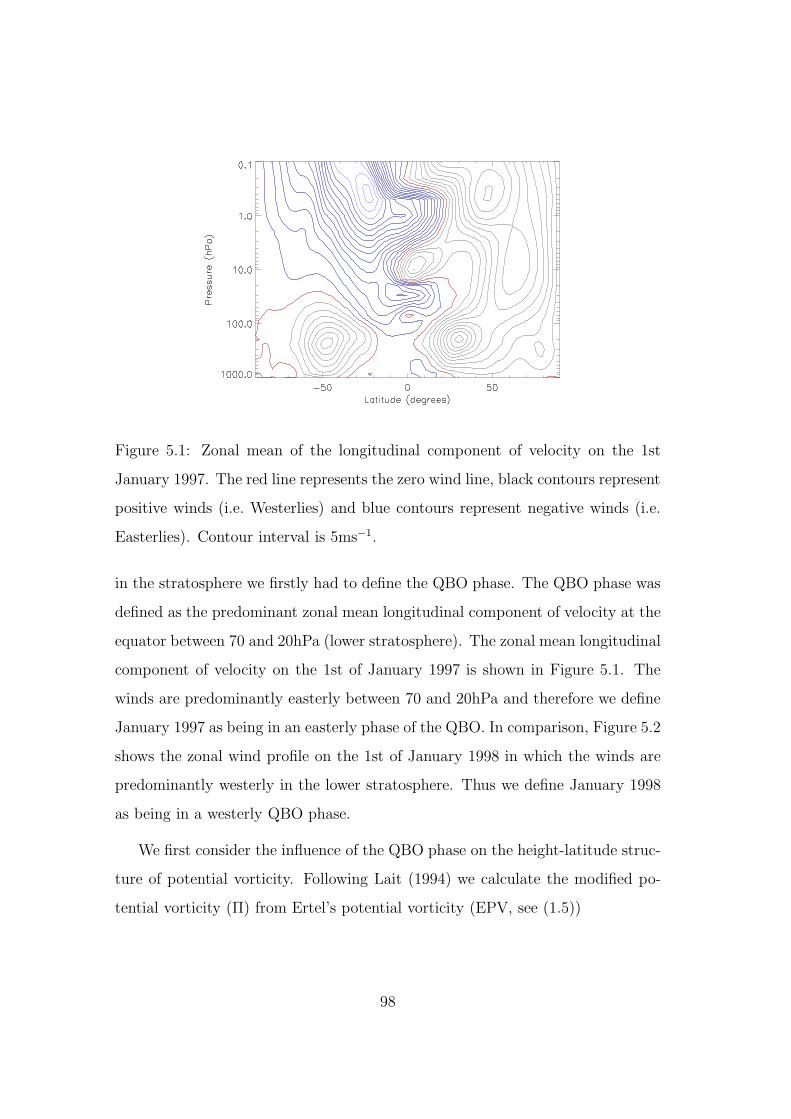
Figure 5.1: Zonal mean of the longitudinal component of velocity on the 1st
January 1997. The red line represents the zero wind line, black contours represent
positive winds (i.e. Westerlies) and blue contours represent negative winds (i.e.
Easterlies). Contour interval is 5ms−1.
in the stratosphere we firstly had to define the QBO phase. The QBO phase was
defined as the predominant zonal mean longitudinal component of velocity at the
equator between 70 and 20hPa (lower stratosphere). The zonal mean longitudinal
component of velocity on the 1st of January 1997 is shown in Figure 5.1. The
winds are predominantly easterly between 70 and 20hPa and therefore we define
January 1997 as being in an easterly phase of the QBO. In comparison, Figure 5.2
shows the zonal wind profile on the 1st of January 1998 in which the winds are
predominantly westerly in the lower stratosphere. Thus we define January 1998
as being in a westerly QBO phase.
We first consider the influence of the QBO phase on the height-latitude struc-
ture of potential vorticity. Following Lait (1994) we calculate the modified po-
tential vorticity (Π) from Ertel’s potential vorticity (EPV, see (1.5))
98

Figure 5.2: Zonal mean of the longitudinal component of velocity on the 1st
January 1998. The red line represents the zero wind line, black contours represent
positive winds (i.e. Westerlies) and blue contours represent negative winds (i.e.
Easterlies). Contour interval is 5ms−1.
Π = EPV
(
θ
θ0
)−92
(5.3)
where θ is the potential temperature and θ0 = 420K is a reference potential
temperature. This removes the exponential vertical dependence of the potential
vorticity enabling us to view its structure in the vertical. The meridional poten-
tial vorticity field (compare Figure 5.3 and Figure 5.4) is significantly different
between the two phases of the QBO. For the years defined as being in an easterly
phase of the QBO there are sharp potential vorticity gradients at the equator
around 70hPa and 10hPa with strong gradients at 20N and 20S between these
two pressure levels. In contrast a westerly QBO phase has very sharp poten-
tial vorticity gradients at the equator up to about 20hPa. Above 20hPa there are
strong potential vorticity gradients in the northern hemisphere subtropics. These
potential vorticity gradients are consistent with the zonal wind fields described
99

above (through potential vorticity inversion: q ∼ k · ∇ × u).
In order to better understand these differences in the vertical structure of the
potential vorticity we investigate its structure on several isentropic surfaces. We
non dimensionalise the potential vorticity following Polvani & Saravanan (2000).
This allows us to use an objective contour interval so that on all isentropic surfaces
we capture the predominant features of the potential vorticity structure. The
modified potential vorticity on each isentropic surface is non dimensionalised by
dividing it by
gκf
p0T01/κθ0
κ+1/κ (5.4)
where κ = 2/7, g = 9.80665, po = 1000hPa, T0 = 240K, θ0 = 420K and f = 2Ω
which is the polar Coriolis parameter where Ω is the Earth’s rotation rate. The
expression in (5.4) has dimensions of potential vorticity (Km2s−1kg−1). The
structure of the potential vorticity on the isentropic surface θ = 580K is shown in
Figure 5.5(a) for the 1st of January 1997 (at the equator θ = 580K corresponds
approximately to 30hPa). Note that these figures seem to be typical for January
(main feature of the potential vorticity structure did not change significantly
over the month). Thermal forcing is fairly constant over winter and therefore we
expect there to be little change in the large-scale potential vorticity structure over
January. Of course if a stratospheric sudden warming occurs there may be more
significant changes to the large-scale potential vorticity structure. We would also
expect differences to occur with changes in season. At θ = 580K (30hPa) the
zonal winds at the equator are easterly and Figure 5.5(a) shows that there are
two regions of strong potential vorticity gradients, one around 20N and 20S
corresponding to the edge of the tropical pipe, the other around 60N at the edge
of the polar vortex.
A useful way of summarising this structure is to define the equivalent latitude
100

of the potential vorticity field (Butchart & Remsberg, 1986). The equivalent
latitude is defined as
φe = sin−1
(
1 −A
2πa2
)
(5.5)
where A is the area in which the potential vorticity is greater than or equal to
q (a particular potential vorticity value) on a given isentropic surface, and a is
the radius of the Earth. The equivalent latitude is the latitude circle (centered
at the pole) that encloses the same area, A. The fact that potential vorticity is
monotonic from pole to pole allows it to be used to define φe. Figure 5.5(b) dis-
plays the potential vorticity on the surface θ = 580K as a function of equivalent
latitude. There are regions of strong potential vorticity gradients around 20N
and 20S indicating the presence of barriers to mixing. These strong potential
vorticity gradients represent the edges of the tropical pipe as discussed earlier.
At higher altitudes on the isentropic surface θ = 860K (at the equator θ = 860K
corresponds approximately to 10hPa) the zonal winds at the equator are west-
erly and the potential vorticity structure on this isentropic surface is significantly
different to that on θ = 580K (see Figure 5.6(a)). Instead of strong potential
vorticity gradients in the subtropics there are strong potential vorticity gradients
at the equator (corresponding to a westerly jet). A cat’s eye structure can be seen
in the extratropics indicating critical layer mixing. The strong potential vortic-
ity gradients at the equator are demonstrated further by the potential vorticity
staircase in Figure 5.6(b) where there is a steep gradient in potential vorticity at
the equator.
Figures 5.7 and 5.8 show the same isentropic surfaces as Figures 5.5 and 5.6
respectively but for January 1998. The difference here is that the zonal winds
at the equator are westerly at θ = 580K and easterly at θ = 860K (i.e. the
opposite of January 1997). There is a clear correlation between the sign of the
zonal winds at the equator on a given level and the structure of the potential
101

vorticity on that same level. At levels where the equatorial winds are easterly
there are strong potential vorticity gradients in the subtropics. At levels where
the equatorial winds are westerly there are strong potential vorticity gradients at
the equator. As explained in section 5.1 strong gradients of potential vorticity
act as barriers to mixing and transport and they form at the edges of critical
layers. We therefore conjecture that when the equatorial winds are easterly the
majority of particles will remain in the tropics and there will be little mixing
from midlatitudes into the tropics. This suggests that the subtropical barrier is
limiting mixing in the northern hemisphere. However when the equatorial winds
are westerly we expect the strong potential vorticity gradients at the equator to
isolate the southern hemisphere from mixing. We also hypothesise that the strong
equatorial potential vorticity gradients will enable particles to mix to the equator
and that particles in the tropics will be mixed out across the northern hemisphere
creating a wide critical layer (see Figures 5.9 and 5.10 for schematics of our
hypothesis). These assumptions are consistent with the work of Shuckburgh
et al. (2001) who found that in a westerly phase of the QBO mixing is enhanced
in the subtropics (we conjecture that mixing is enhanced to the equator) and in
an easterly phase mixing is inhibited in the tropics. It is important to note that
the edge of the tropical pipe is only well defined in terms of potential vorticity
gradients on levels where the zonal winds are easterly. On levels where the
zonal winds are westerly there are no strong potential vorticity gradients in the
subtropics. Therefore the edge of the tropical pipe may not be well defined there.
Finally the potential vorticity gradients are stronger in the northern hemisphere,
consistent with vigorous mixing occurring in the surf zone.
5.2.3 Experiment Design
To test our hypothesis we examine mixing and lateral transport in the winter
stratosphere. More specifically we begin with Januarys in either an easterly or
102

Figure 5.3: Zonal mean potential vorticity, with the vertical dependence removed,
on the 1st January 1997. Contour interval is 5x10⁻⁷Km2s−1kg−1. Easterly QBO.
Figure 5.4: Zonal mean potential vorticity, with the vertical dependence removed,
on the 1st of January 1998. Contour interval is 5x10⁻⁷Km2s−1kg−1. Westerly
QBO.
103
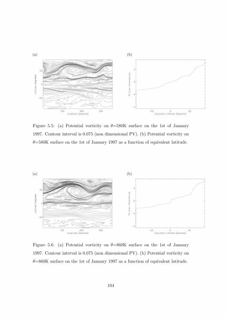
(a) (b)
Figure 5.5: (a) Potential vorticity on θ=580K surface on the 1st of January
1997. Contour interval is 0.075 (non dimensional PV). (b) Potential vorticity on
θ=580K surface on the 1st of January 1997 as a function of equivalent latitude.
(a) (b)
Figure 5.6: (a) Potential vorticity on θ=860K surface on the 1st of January
1997. Contour interval is 0.075 (non dimensional PV). (b) Potential vorticity on
θ=860K surface on the 1st of January 1997 as a function of equivalent latitude.
104

(a) (b)
Figure 5.7: (a) Potential vorticity on θ=580K surface on the 1st of January
1998. Contour interval is 0.075 (non dimensional PV). (b) Potential vorticity on
θ=580K surface on the 1st of January 1998 as a function of equivalent latitude.
(a) (b)
Figure 5.8: (a) Potential vorticity on θ=860K surface on the 1st of January
1998. Contour interval is 0.075 (non dimensional PV). (b) Potential vorticity on
θ=860K surface on the 1st of January 1998 as a function of equivalent latitude.
105

SP Equator NP
20
70
100
Pres
sure
(hP
a)
Polar Vortex
mixing
mixing
Figure 5.9: Schematic of our hypothesis for our definition of Easterly QBO Jan-
uary’s.
SP Equator NP
20
70
100
Pres
sure
(hP
a)
Polar Vortex
mixing
mixing
Figure 5.10: Schematic of our hypothesis for our definition of Westerly QBO
January’s.
106
westerly phase of the QBO. To reduce the effects of large interannual variability
the three most extreme Januarys in each QBO phase between the years 1979
and 1998 were selected. This gave January 1983, 1989 and 1997 as the three
easterly QBO winters and January 1984, 1995 and 1998 as the three westerly QBO
winters. Strong easterly or westerly QBO phases represent extreme conditions
within the tropics.
The model used is the “online” trajectory model described in chapter 4. The
Lagrangian particles are initialised on ten vertical levels in the stratosphere,
namely 150, 100, 70, 50, 30, 20, 15, 10, 7 and 5 hPa. On each vertical level
the particles are initially distributed so that the area between two adjacent par-
ticles on one latitude and the two adjacent particles on the adjacent latitude
is approximately equal. The particles are spaced every 1.25 in latitude from
88.75N to 88.75S. At the equator particles are spaced every 1.875 in longitude.
The number of particles on each latitude circle then decreases towards the poles
in order to conserve the area between them. This results in 17,600 particles on
each vertical level and therefore there are 176,000 particles in total. The parti-
cles are initialised on the 1st of January for each of the six January’s studied.
They are advected until the 10th of February and, as section 5.3 will demon-
strate, forty days is sufficient to capture significant mixing and transport in the
wintertime stratosphere. Temperature, water vapour and potential vorticity are
assigned as attributes to the particles (see chapter 4). Potential vorticity as an
attribute is particularly important as it will allow us to know where particles are
in relation to the potential vorticity field of the flow at any given time. Since
potential vorticity is materially conserved for a conservative flow, changes in the
trajectory potential vorticity represent the effects of non-conservative processes
(e.g. dissipation from small-scale mixing).
107

5.3 Analysis of Trajectories
In this section we analyse the trajectories of Lagrangian particles with a spe-
cific focus on the differences between QBO phases. We follow particles that are
initially on levels where the equatorial zonal winds are easterly or westerly. Fig-
ure 5.11 displays the levels of particular focus in this analysis which are 30hPa
and 10hPa. In the easterly QBO winters the equatorial zonal winds are easterly
at 30hPa and westerly at 10hPa. The opposite is true for the westerly QBO
winters. Note that at the equator 30hPa corresponds closely to the θ = 580K
isentropic surface (see Figures 5.5 and 5.7 for the potential vorticity structure on
this surface) and 10hPa corresponds closely to the θ = 860K isentropic surface
(see Figures 5.6 and 5.8). To examine mixing and transport out of the tropics
(and thus test our hypothesis) we chose to divide the tropics into equivalent lat-
itude intervals that were fractions of a subtropical equivalent latitude, denoted
by φp. At levels where the equatorial zonal winds are easterly φp is taken to be
the equivalent latitude of the strongest potential vorticity gradient in the sub-
tropics (φp varies from 19.4 to 29.1). However at levels where the equatorial
zonal winds are westerly there are no strong potential vorticity gradients in the
subtropics and therefore φp = 23 is chosen as a suitable subtropical latitude.
We then follow particles that initially have an equivalent latitude, φe, within
intervals of 14φp (e.g. 3
4φp ≤ φe ≤ φp,
12φp ≤ φe ≤ 3
4φp etc. ) and then count
how many of those particles have an equivalent latitude greater than φp at some
later time T. To determine the equivalent latitude of the particles at time, T, we
compare the potential vorticity of the particle (potential vorticity attribute) with
the potential vorticity of the flow. In order to make this comparison we must
compare the same form of potential vorticity. In terms of the flow we know the
non-dimensional potential vorticity on isentropic surfaces (see section 5.2.2) and
can therefore determine the non-dimensional potential vorticity associated with
each equivalent latitude of interest, for example φp,34φp,
12φp etc. (see Figures 5.5
108

to 5.8). Using the expression in (5.4) we calculate the modified potential vorticity
associated with each equivalent latitude. We also convert the potential vorticity
attributed to each particle into modified potential vorticity (5.3) and therefore
we know where the particle is in relation to a given equivalent latitude. Note that
the modified potential vorticity removes the exponential vertical dependence of
potential vorticity allowing us to determine the particles positions with respect
to specific equivalent latitudes independent of their movement in the vertical.
The percentage of particles that have moved outside the tropics by day 5, 10,
20 and 40 of the trajectory calculation (averaged over the three winters in that
QBO phase) are displayed in Tables 5.1 to 5.4. Each table contains the values
for particles initially on a given pressure level (either 30hPa or 10hPa) and for a
given winter defined to be in an easterly or westerly QBO phase (January 1997 &
1998). Comparing Tables 5.1 and 5.2 for the easterly QBO winters demonstrates
that there is greater mixing out of the tropics at higher altitudes (10hPa), where
the equatorial zonal winds are westerly, than at lower altitudes (30hPa), where
the winds are easterly. This agrees with our hypothesis (Figure 5.9) as the strong
subtropical gradients of potential vorticity at 30hPa apparently inhibit transport
out of the tropics. Table 5.1 suggests that particles have to be well within the
tropics, say 14φp ≤ φe ≤ 1
2φp, on levels where the equatorial zonal winds are
easterly before transport is reduced significantly by the strong potential vorticity
gradients in the subtropics. This may be because particles initially with an equiv-
alent latitude greater than 12φp are within the band of strong potential vorticity
gradients in the subtropics and are therefore not equatorward of the barrier to
mixing and transport. Hence they are more easily mixed out of the tropics.
Figure 5.12(a) shows the particles initially on 30hPa at 14φp ≤ φe ≤ 1
2φp on
the 1st January 1997 and then their positions at T = 40 days are shown in
Figure 5.12(b). Note that the black contour in these figures and the subsequent
trajectory figures is the modified potential vorticity contour with an equivalent
109

latitude φp at time T. At T = 40 days it is clear that some particles have been
mixed out of the tropics and have started to descend. Also the particles that
have remained in the tropics have mixed across tropical latitudes. This is more
evident in Figure 5.13 which is the same as Figure 5.12 except that the particles
are initially between the equator and 14φp. Contrasting Figures 5.13(a) and (b)
it is evident that in this case particles are being mixed across the tropics with
some being transported southward of the equator.
In contrast to Figure 5.12, Figure 5.14 shows particles initially between 14φp
and 12φp on 10hPa where the equatorial zonal winds are westerly rather than on
30hPa (easterly QBO phase). In Figure 5.14(b) particles that have been trans-
ported out of the tropics have been mixed right across the northern hemisphere.
The movement of particles initially between the equator and 14φp on 10hPa is
shown in Figure 5.15. In this case the majority of particles remain at the equator
(Figure 5.15(b)). On 10hPa, where the equatorial zonal winds are westerly, there
are strong potential vorticity gradients at the equator which trap particles there.
This implies that there is a barrier to mixing and transport at the equator on
levels where the equatorial zonal winds are westerly. Also a comparison between
pressure levels in Figures 5.13 and 5.15 shows a noticeable difference in the par-
ticles positions at T = 40 days which demonstrates the difference in transport
between QBO phases.
A comparison of Tables 5.3 and 5.4 for the westerly QBO winters does not
show a clear decrease in mixing between 30hPa and 10hPa as we would have
expected from our hypothesis. There is a slight decrease in the percentage of
particles transported to latitudes greater than φp at T = 20 days (from 39.6% on
30hPa to 32.2% on 10hPa) for particles initially between 12φp and 3
4φp. However
by T = 40 days the percentage of escaped particles is greater on 10hPa than
on 30hPa for all initial positions of particles. Comparing Figures 5.16 and 5.18
at T = 40 days does not show a clear decrease in the amount of particles that
110
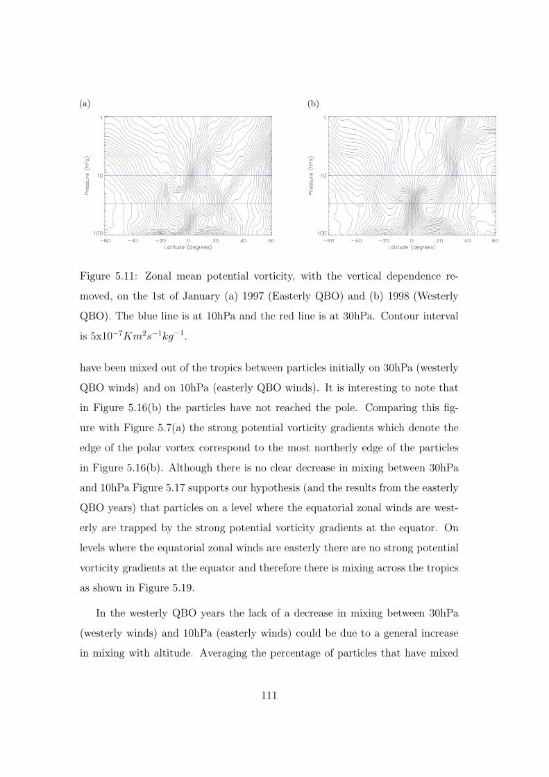
(a) (b)
Figure 5.11: Zonal mean potential vorticity, with the vertical dependence re-
moved, on the 1st of January (a) 1997 (Easterly QBO) and (b) 1998 (Westerly
QBO). The blue line is at 10hPa and the red line is at 30hPa. Contour interval
is 5x10⁻⁷Km2s−1kg−1.
have been mixed out of the tropics between particles initially on 30hPa (westerly
QBO winds) and on 10hPa (easterly QBO winds). It is interesting to note that
in Figure 5.16(b) the particles have not reached the pole. Comparing this fig-
ure with Figure 5.7(a) the strong potential vorticity gradients which denote the
edge of the polar vortex correspond to the most northerly edge of the particles
in Figure 5.16(b). Although there is no clear decrease in mixing between 30hPa
and 10hPa Figure 5.17 supports our hypothesis (and the results from the easterly
QBO years) that particles on a level where the equatorial zonal winds are west-
erly are trapped by the strong potential vorticity gradients at the equator. On
levels where the equatorial zonal winds are easterly there are no strong potential
vorticity gradients at the equator and therefore there is mixing across the tropics
as shown in Figure 5.19.
In the westerly QBO years the lack of a decrease in mixing between 30hPa
(westerly winds) and 10hPa (easterly winds) could be due to a general increase
in mixing with altitude. Averaging the percentage of particles that have mixed
111

Table 5.1: The Average Percentage of Particles with φe > φp at Several Times for
the Easterly QBO Years; particles initially at 30hPa (easterly equatorial winds).
Particles Initial Positions
Day 34φp ≤ φe ≤ φp
12φp ≤ φe ≤
34φp
14φp ≤ φe ≤
12φp 0 ≤ φe ≤
14φp -1
4φp ≤ φe ≤ 0
5 19.8 4.4 0.2 0.0 0.0
10 30.8 10.6 0.4 0.0 0.0
20 40.4 19.6 2.1 1.1 0.3
40 62.4 39.4 22.3 11.7 2.3
Table 5.2: The Average Percentage of Particles with φe > φp at Several Times for
the Easterly QBO Years; particles initially at 10hPa (westerly equatorial winds).
Particles Initial Positions
Day 34φp ≤ φe ≤ φp
12φp ≤ φe ≤
34φp
14φp ≤ φe ≤
12φp 0 ≤ φe ≤
14φp -1
4φp ≤ φe ≤ 0
5 28.9 6.4 1.4 0.0 0.0
10 41.7 18.7 4.2 0.1 0.0
20 57.9 39.6 16.9 0.9 0.0
40 73.3 49.4 26.3 1.0 0.0
out of the tropics for a given initial pressure level over all six years (not shown)
demonstrates that there is indeed a weak increase in mixing with altitude. There-
fore although in the westerly QBO years the QBO phase may inhibit mixing at
high altitudes, this is apparently offset by the increase in mixing with altitude.
In the easterly QBO years the increase in mixing with altitude from a level where
the winds are easterly to a level where the winds are westerly will be accentuated
by the QBO structure which will inhibit mixing at lower altitudes. Furthermore,
although there is variability in the six years examined all the years demonstrate
a weak dependence on mixing with altitude (possibly due to larger amplitude
Rossby wave breaking at higher altitudes). In addition to a general increase in
112

Table 5.3: The Average Percentage of Particles with φe > φp at Several Times
for the Westerly QBO Years; particles at 30hPa (westerly equatorial winds).
Particles Initial Positions
Day 34φp ≤ φe ≤ φp
12φp ≤ φe ≤
34φp
14φp ≤ φe ≤
12φp 0 ≤ φe ≤
14φp -1
4φp ≤ φe ≤ 0
5 31.6 7.8 2.0 0.0 0.0
10 40.8 19.2 5.4 0.0 0.0
20 50.9 39.6 9.6 0.0 0.0
40 62.4 55.0 25.3 1.2 0.0
Table 5.4: The Average Percentage of Particles with φe > φp at Several Times for
the Westerly QBO Years; particles initially at 10hPa (easterly equatorial winds).
Particles Initial Positions
Day 34φp ≤ φe ≤ φp
12φp ≤ φe ≤
34φp
14φp ≤ φe ≤
12φp 0 ≤ φe ≤
14φp -1
4φp ≤ φe ≤ 0
5 25.4 6.3 2.4 0.8 0.0
10 40.5 15.4 5.2 1.9 0.0
20 52.1 32.2 15.7 10.5 1.0
40 68.2 57.1 34.3 18.6 2.8
mixing with altitude there is a dependence of the out-mixing on the time integra-
tion of the trajectory code. This is to be expected due to the chaotic nature of
trajectories since in general particles will experience more mixing and transport
over longer trajectories. Also as particles are initialised closer to the equator the
percentage of particles escaping to latitudes greater than φp generally decreases
and drops significantly between different bands of initial particles depending on
whether the equatorial zonal winds are easterly or westerly.
Finally we compare the mixing and transport at 30hPa when the equatorial
zonal winds are easterly (Table 5.1) and when they are westerly (Table 5.3).
This comparison shows that up to T = 20days the percentage of particles that
113

(a) (b)
Figure 5.12: Particle positions at (a) t = 0 and (b) t = 40 days. Particles are
initially on 30hPa at 14φp ≤ φe ≤ 1
2φp on the 1st January 1997. Note: Zonal
winds at the equator are easterly on 30hPa.
are mixed out of the tropics when the winds are westerly is approximately double
the percentage mixed out of the tropics when the winds are easterly. Making
a similar comparison for particles initially on 10hPa (Tables 5.2 and 5.4) indi-
cates a slight increase in mixing out of the tropics (at T = 40 days) when the
equatorial zonal winds are easterly. This is counter to our expectations from our
hypothesis which states that when the equatorial zonal winds are easterly the
strong potential vorticity gradients in the subtropics limit mixing in the northern
hemisphere. Is it possible that the fact that mixing increases with altitude is
causing a comparison at this altitude to become less well defined? Considering
only the levels where the equatorial zonal winds are easterly (Tables 5.1 and 5.4)
reveals a significant increase in mixing out of the tropics at 10hPa over that at
30hPa. This suggests that the increase in mixing at higher altitudes may break
or weaken the subtropical barrier by T = 20 days leading to a marked increase
in mixing and transport out of the tropics. This therefore makes it difficult to
compare mixing and transport between easterly and westerly QBO phases at high
altitudes.
114

(a) (b)
Figure 5.13: Particle positions at (a) t = 0 and (b) t = 40 days. Particles are
initially on 30hPa at 0 ≤ φe ≤14φp on the 1st January 1997. Note: Zonal winds
at the equator are easterly on 30hPa.
(a) (b)
Figure 5.14: Particle positions at (a) t = 0 and (b) t = 40 days. Particles are
initially on 10hPa at 14φp ≤ φe ≤ 1
2φp on the 1st January 1997. Note: Zonal
winds at the equator are westerly on 10hPa.
115
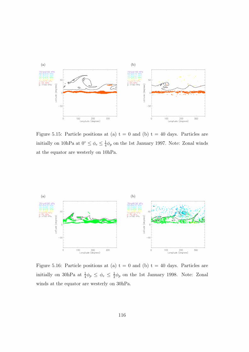
(a) (b)
Figure 5.15: Particle positions at (a) t = 0 and (b) t = 40 days. Particles are
initially on 10hPa at 0 ≤ φe ≤14φp on the 1st January 1997. Note: Zonal winds
at the equator are westerly on 10hPa.
(a) (b)
Figure 5.16: Particle positions at (a) t = 0 and (b) t = 40 days. Particles are
initially on 30hPa at 14φp ≤ φe ≤ 1
2φp on the 1st January 1998. Note: Zonal
winds at the equator are westerly on 30hPa.
116

(a) (b)
Figure 5.17: Particle positions at (a) t = 0 and (b) t = 40 days. Particles are
initially on 30hPa at 0 ≤ φe ≤14φp on the 1st January 1998. Note: Zonal winds
at the equator are westerly on 30hPa.
(a) (b)
Figure 5.18: Particle positions at (a) t = 0 and (b) t = 40 days. Particles are
initially on 10hPa at 14φp ≤ φe ≤ 1
2φp on the 1st January 1998. Note: Zonal
winds at the equator are easterly at 10hPa.
117

(a) (b)
Figure 5.19: Particle positions at (a) t = 0 and (b) t = 40 days. Particles are
initially on 10hPa at 0 ≤ φe ≤14φp on the 1st January 1998. Note: Zonal winds
at the equator are easterly at 10hPa.
5.3.1 In-Mixing
The focus of this chapter has been on the effect of the QBO phase on lateral
mixing and transport out of the tropics. However mixing from the surf zone
into the tropics is also important as this changes tracer concentrations within
the tropical pipe. Note that no such change in tracer concentrations occurs with
out-mixing. It therefore has implications for the transport of chemicals such as
ozone and water vapour in the stratosphere. To determine whether there is a
difference in in-mixing with QBO phase we examine the movement of particles
initially on 30hPa with an equivalent latitude greater than φp. This was carried
out for both January 1997 (where the equatorial zonal winds are easterly) and
January 1998 (where the equatorial zonal winds are westerly) (Figures 5.20 and
5.21). Note that the particles are initialised so that the area between them is
conserved and hence there are less particles at the poles than at the equator
and this is the reason for the pattern observed in Figures 5.20(a) and 5.21(a).
The percentage of particles initially north of the tropics that are mixed into the
tropics (for both January 1997 and 1998) are displayed in Table 5.5. In the case
where the QBO phase is easterly there is not much difference in the percentage
118

of in-mixing over time and the percentage value is very small. This suggests that
the strong potential vorticity gradients in the subtropics are stronger barriers to
in-mixing than to mixing out of the tropics. Another contributor to this could be
the vigorous mixing of the extratropical surf zone which entrains particles from
the tropics. On the other hand when the QBO phase is westerly the percentage
of particles mixed into the tropics increases with time to a maximum of 17.7%
at T = 40days. This again supports our hypothesis that the strong potential
vorticity gradients at the equator on levels where the equatorial zonal winds are
westerly enables mixing to occur from the equator to the polar vortex.
This analysis is simply an example of the effect of the QBO phase on mixing
into the tropics. We leave further consideration of this topic for future work.
Table 5.5: The Percentage of Particles Initially Outside the Tropics on 30hPa
that move into the Tropics after time t.
Day January 1997 (Easterly) January 1998 (Westerly)
5 3.0 5.3
10 3.2 6.8
20 4.4 11.1
40 2.7 17.7
5.4 Discussion
In this chapter we have investigated the effect of the QBO on transport and
mixing in the stratosphere. We have shown that the phase of the QBO affects
the structure of potential vorticity in the stratosphere. At levels where the QBO
phase is westerly there are strong potential vorticity gradients at the equator
which trap particles there, implying an equatorial barrier. Also these strong
gradients enable mixing from between just north of the equator to the polar
119
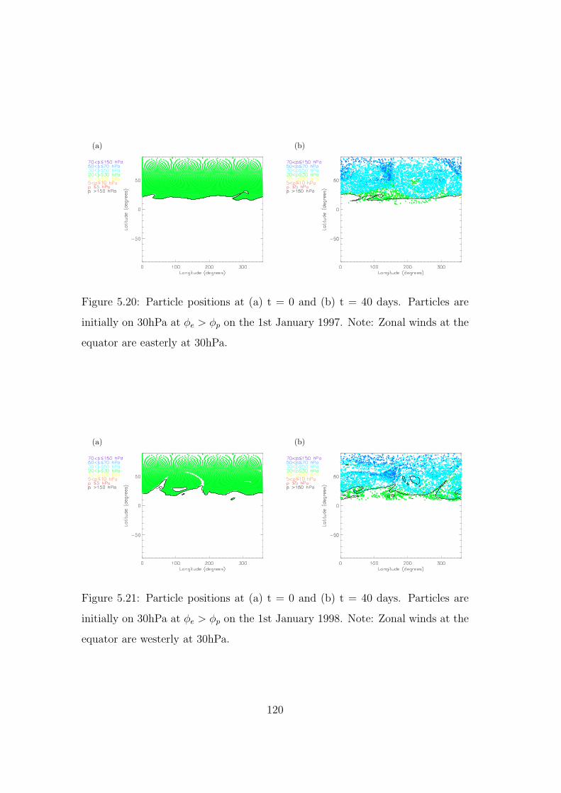
(a) (b)
Figure 5.20: Particle positions at (a) t = 0 and (b) t = 40 days. Particles are
initially on 30hPa at φe > φp on the 1st January 1997. Note: Zonal winds at the
equator are easterly at 30hPa.
(a) (b)
Figure 5.21: Particle positions at (a) t = 0 and (b) t = 40 days. Particles are
initially on 30hPa at φe > φp on the 1st January 1998. Note: Zonal winds at the
equator are westerly at 30hPa.
120

vortex allowing particles from the extratropics to mix into the tropics. Conversely
at levels where the QBO phase is easterly there are strong potential vorticity
gradients in the subtropics. These potential vorticity gradients act as barriers
to mixing, albeit weaker barriers than the potential vorticity gradients at the
equator in the westerly QBO phase levels. These subtropical gradients limit the
mixing region in the northern hemisphere to between the subtropics and the polar
vortex. Also there is mixing across the tropics at the levels where the QBO phase
is easterly. These results are consistent to those of Shuckburgh et al. (2001) who
found that mixing is inhibited in the tropics during an easterly phase of the QBO
and that during a westerly phase mixing is enhanced in the subtropics.
Following the work of Plumb (1996) the region above the tropical tropopause
is referred to as the tropical pipe with the edges of the tropical pipe acting as
barriers to mixing. From this investigation if appears that it may be more of a
broken pipe. At the levels where the QBO phase is easterly the strong potential
vorticity gradients in the subtropics can be regarded as the edges of the tropical
pipe. However on levels where the equatorial zonal winds are westerly the strong
potential vorticity gradients at the equator enable mixing from the equator to
the pole and therefore the tropical pipe terminology is perhaps less applicable in
this case.
In this chapter we have also considered the effect of the QBO phase on mixing
and lateral transport into the tropics. We have demonstrated that significantly
more in-mixing occurs when the equatorial zonal winds are westerly due to the
strong potential vorticity gradients at the equator enabling mixing to occur from
the equator to the polar vortex. When the QBO phase is easterly we found very
little in-mixing into the tropics. This suggests that the strong potential vorticity
gradients in the subtropics are strong barriers to in-mixing.
This analysis has allowed us to conjecture how the different QBO phases affect
where the particles go in terms of ascent. In a westerly QBO year we expect more
121

particles to be mixed out towards the pole, where they begin to descend, than to
ascend in the tropics to higher altitudes (weak upwelling). On the other hand in
an easterly QBO year we expect more particles to remain in the tropics reaching
higher altitudes (strong upwelling) at which point the winds are westerly and they
will be transported towards the pole and begin to descend. The work of Punge
et al. (2009), who considered the effect of the QBO on stratospheric transport
at low latitudes using trajectory calculations from a general circulation model,
supports this ascent conjecture. They found that upwelling in the tropics was
enhanced when the equatorial winds were easterly and that this was reduced in
a westerly QBO phase. This difference in ascent due to the dependence of lateral
mixing on the QBO phase could have an influence on the ascent of chemicals such
as ozone and water vapour and therefore affect the processes they are involved
in in the stratosphere.
The phase of the QBO affects the lateral mixing and transport in the strato-
sphere. Understanding atmospheric transport and mixing is of particular im-
portance to geoengineers who are considering injecting aerosols into the lower
stratosphere to balance the effects of climate change. The affect of the QBO
phase on mixing and transport in the stratosphere will play a vital role in this
area of meteorology. This chapter has focused on mixing and transport out of
the tropics. In future we could use this trajectory model to give further consid-
eration to mixing into the tropics and the effect on chemical concentrations and
transport in the stratosphere.
122
Chapter 6
Conclusions
The focus of this thesis has been an investigation of the transport and critical
layer mixing in the troposphere and stratosphere. The understanding of this
transport and mixing is important because it affects our weather and climate.
Chapter 1 summarised the structure of the atmosphere and the main dy-
namics that occur in the troposphere and stratosphere. Diagnostics to quantify
mixing and transport were introduced such as Lyapunov exponents and effective
diffusivity. A brief review of recent work involving effective diffusivity was given
followed by an explanation of the calculation of this diagnostic.
In chapter 2 we investigated the evolution of a Rossby wave critical layer in
an idealised model (channel model). Our work differed from that of SWW (1978)
and Haynes (1989) in that we force the streamfunction in the critical layer di-
rectly. We examined the effect of the shear across the critical layer on the critical
layer evolution, and more specifically on the development of barotropic instability
in the critical layer. We found (consistent with Haynes (1989)) that barotropic
instability occurred when the shear was suitably small, Λ ≤ 0.3. We also consid-
ered how the mixing efficiency of the critical layer depended on the shear across
the critical layer and used this dynamically consistent flow to compare different
123

measures of mixing (effective diffusivity and contour lengths). The mixing effi-
ciency of the critical layer increased due to barotropic instability and effective
diffusivity and contour lengths were found to be consistent measures of mixing.
Barotropic instability was found to enhance mixing in the critical layer at early
times when the shear was small. However this enhancement was much smaller
than the enhancement of mixing due to the resonant growth of the critical layer
around Λ = 12.
In an extension to previous work a systematic investigation of the critical layer
evolution at finite Rossby deformation length was carried out. This investigation
was set up so that as far as possible everything was the same as the infinite
Rossby deformation length investigation, i.e. topographic forcing and average
shear in the critical layer region (same closed streamline pattern). We found that
regardless of this the critical layer width increased at small LD. This was due to
the effect of LD on the Rossby wave elasticity. We therefore chose to estimate
the growth of the critical layer width with decreasing LD. We discovered that at
small LD, LD less than the natural wavelength of the instability, the wavelength
of the instability reduces.
In chapter 3 we found that changes to the stratospheric potential vortic-
ity have a significant impact on the development of baroclinic instability in an
Eady-like model. The dependence is such that increasing the strength of the polar
vortex tends to decrease the eddy growth in the troposphere. This is found not
just in the zonally symmetric cases, comparing zonally symmetric stratospheric
perturbations of different potential vorticity magnitudes, but also in cases of zon-
ally asymmetric disturbances to a polar vortex of given potential vorticity. The
latter scenario extends previous work that had considered only zonally symmetric
stratospheric perturbations. In particular, we found that there is a large differ-
ence in the tropospheric evolution between cases representing a strong vortex
and cases representing the vortex following either a wave-one or wave-two sud-
124

den warming. Differences in the tropospheric evolution include the growth of
eddy kinetic energy and wave activity, as well as synoptic scale details of the
wave breaking and the latitudinal extent of mixing within the troposphere. One
of the important results of this work is that the potential vorticity perturbations
made here result in significantly larger differences to the tropospheric evolution
than obtained by perturbations to the stratospheric winds alone.
One significant difference between our results and those of Wittman et al.
(2004, 2007) is the sense in which a stratospheric perturbation affects the growth
of the instability. Wittman et al. found an increase in eddy growth rates with
increasing stratospheric shear, whereas we find a decrease in growth rates with
increasing stratospheric potential vorticity. The results are not inconsistent when
full account is taken of changes to the tropospheric shear resulting from the
stratospheric potential vorticity perturbation in our case, which tends to leave
the vertical shear unchanged but increases the horizontal shear. The decrease in
growth rates we observed may therefore be attributed to a change in the nature of
the baroclinic development similar to that found by Thorncroft et al. (1993). One
conclusion that may be drawn from both Wittman et al. and the present work
is that the tropospheric evolution depends rather sensitively on the stratospheric
state through details of the shear in the troposphere and near the subtropical jet.
Chapter 4 described a trajectory model, developed in conjunction with the
UK Met Office, called the “online” trajectory code. This chapter gave a brief
outline of the model followed by the results of some sensitivity experiments. This
trajectory model is then used to study atmospheric transport and mixing in the
stratosphere in more realistic situations.
In chapter 5 we investigated the effect of the QBO on transport and mixing
in the stratosphere using the trajectory model described in chapter 4. We have
shown that the phase of the QBO affects the structure of potential vorticity in
the stratosphere. At levels where the QBO phase is westerly there are strong
125

potential vorticity gradients at the equator which trap particles there. Also these
strong gradients enable mixing to occur from between just north of the equator to
the polar vortex allowing particles from the extratropics to mix into the tropics.
Conversely at levels where the QBO phase is easterly there are strong potential
vorticity gradients in the subtropics. These potential vorticity gradients act as
barriers to mixing, albeit weaker barriers than the potential vorticity gradients at
the equator in the westerly QBO phase levels. These subtropical gradients limit
the mixing region in the northern hemisphere to between the subtropics and the
polar vortex.
We have considered everything in terms of potential vorticity and we have
found that the phase of the QBO affects the potential vorticity structure. The
waves that drive the QBO are predominantly Kelvin waves and don’t have po-
tential vorticity themselves. Consequently the effect on potential vorticity is not
obvious. However they do have an effect on the mean flow and therefore the
shear. In chapter 2 (using an idealised model) we examined the effect of the
shear across a critical layer on the critical layer evolution. We found that the
shear alters the efficiency of mixing in the critical layer and that as the shear re-
duces the critical layer width increases. Therefore if we consider the effect of the
QBO on the horizontal shear the potential vorticity structure associated with a
particular phase of the QBO could be the result of critical layer mixing where the
critical layer width and the development of barotropic instability depend upon
the shear. When the QBO phase is westerly the horizontal shear decreases (see
Figure 5.2 - the shear at 20N is weaker in the subtropics at the height of the
westerlies than at the height of the easterlies) which results in an increase in
the critical layer width and therefore allows transport to occur from the equator
to the pole. This connection between these works highlights a link between the
horizontal shear, the critical layer width and the extent of the particle mixing.
Following the work of Plumb (1996) the region above the tropical tropopause
126
is referred to as the tropical pipe with the edges of the tropical pipe acting as
barrier to mixing. From this investigation if appears that it may be more of a
broken pipe. At the levels where the QBO phase is easterly the strong potential
vorticity gradients in the subtropics can be regarded as the edges of the tropical
pipe. However on levels where the equatorial zonal winds are westerly the strong
potential vorticity gradients at the equator enable mixing from the the equator
to the pole and therefore the tropical pipe terminology is perhaps less applicable
in this case.
Finally we also considered the effect of the QBO phase on mixing and lateral
transport into the tropics. We demonstrated that significantly more in-mixing
occurs when the equatorial zonal winds are westerly due to the strong potential
vorticity gradients at the equator enabling mixing to occur from the equator to
the polar vortex. When the QBO phase is easterly we found very little in-mixing
into the tropics. This suggests that the strong potential vorticity gradients in
the subtropics are strong barriers to in-mixing. The affect of the QBO phase on
lateral mixing and transport in the stratosphere is essential for understanding
tracer transport in the atmosphere.
127

Chapter 7
Appendix: Online Trajectory
Code
7.1 Where to Find the Online Code and How
to Use It
The online trajectory code can be found at the UK Met Office in the directory
/project/strat anl/traj online. The online trajectory code currently runs on ver-
sion 7.3 of the Unified Model. To run the online trajectory code a branch of the
Unified Model must be created and the following files committed to the branch
(in the branches directory /src/control/top level):
/project/strat anl/traj online/u model.F90
/project/strat anl/traj online/traj mod.F90
/project/strat anl/traj online/trajmain.F90
/project/strat anl/traj online/traj online.F90
/project/strat anl/traj online/UMVARS.h
/project/strat anl/traj online/TIMEV.h
128

/project/strat anl/traj online/RESPECTR.h
/project/strat anl/traj online/PATH.h
/project/strat anl/traj online/PARAM2.h
/project/strat anl/traj online/PARAM1.h
/project/strat anl/traj online/LEGAUGS.h
/project/strat anl/traj online/LEGAU.h
/project/strat anl/traj online/GRIDP.h
/project/strat anl/traj online/COMPSG.h
/project/strat anl/traj online/COMGRM.h
/project/strat anl/traj online/COMFFT.h
/project/strat anl/traj online/CLUSTERS.h
/project/strat anl/traj online/CHANS.h
/project/strat anl/traj online/BLANK.h
The online trajectory code currently requires the U and V components of
the velocity on pressure levels, omega
(
dp
dt
)
on pressure levels, surface pressure,
temperature on pressure levels, potential vorticty on pressure levels and specific
humidity on pressure levels.
7.2 Information on Parameters
The code “trajmain.F90” gets the required global fields (for the trajectory
calculation) from the D1 array and then passes these global fields into the tra-
jectory code, “traj online.F90”, to calculate particle trajectories. A module
“traj mod.F90” is used by “trajmain.F90” to specify the total number of global
fields required from the D1 array and whether they are prognostic fields or diag-
nostic fields. The parameters used in “traj mod.F90” are listed in Table 7.1.
Note that if different vertical coordinates were used or different attributes
129

Table 7.1: Parameters used to specify the global fields required by the online
trajectory code.
Name Value Description
Ntraj D1items 7 Total number of global fields required
n in progs 0 Number of prognostic fields
n in diags0 1 Number of diagnostics from section 0 of the UM
n in diags15 1 Number of diagnostics from section 15 of the UM
n in diags30 5 Number of diagnostics from section 30 of the UM
to the particles were chosen then the parameters in Table 7.1 would need to be
amended in “traj mod.F90” so they were correct for the global fields required.
Also any different required global fields need to be defined in “traj mod.F90” in
terms of their item number and their dimensions.
In “trajmain.F90” the number of vertical levels is hardwired into the code,
pressure levels= 31. Therefore any change to the number of levels in the vertical
and this part of “trajmain.F90” will need to be addressed. Also in “trajmain.F90”
the arrays of the global fields at the current timestep are called U global, V global,
temp global, omega global, pstar global, PV global and wvap global (Note that
the global fields at the previous timestep are U global last, V global last, etc. ).
Consequently any additional meteorological fields attributed to the particles will
need to be named in this way and passed into “traj online.F90” with their item
number specified in the subroutine GETD1FLDS GLOBAL.
In “traj online.F90” the 31 pressure levels are hardwired into an array called
plev in the subroutine INIUM. This is not ideal but during this project our focus
was on the science and therefore this was sufficient. In the future, of course, we
will aim to make the code more general.
The header files contain important parameters such as the number of particles
130
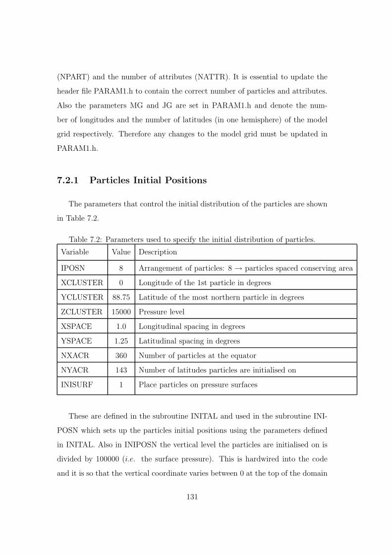
(NPART) and the number of attributes (NATTR). It is essential to update the
header file PARAM1.h to contain the correct number of particles and attributes.
Also the parameters MG and JG are set in PARAM1.h and denote the num-
ber of longitudes and the number of latitudes (in one hemisphere) of the model
grid respectively. Therefore any changes to the model grid must be updated in
PARAM1.h.
7.2.1 Particles Initial Positions
The parameters that control the initial distribution of the particles are shown
in Table 7.2.
Table 7.2: Parameters used to specify the initial distribution of particles.
Variable Value Description
IPOSN 8 Arrangement of particles: 8 → particles spaced conserving area
XCLUSTER 0 Longitude of the 1st particle in degrees
YCLUSTER 88.75 Latitude of the most northern particle in degrees
ZCLUSTER 15000 Pressure level
XSPACE 1.0 Longitudinal spacing in degrees
YSPACE 1.25 Latitudinal spacing in degrees
NXACR 360 Number of particles at the equator
NYACR 143 Number of latitudes particles are initialised on
INISURF 1 Place particles on pressure surfaces
These are defined in the subroutine INITAL and used in the subroutine INI-
POSN which sets up the particles initial positions using the parameters defined
in INITAL. Also in INIPOSN the vertical level the particles are initialised on is
divided by 100000 (i.e. the surface pressure). This is hardwired into the code
and it is so that the vertical coordinate varies between 0 at the top of the domain
131

and one at the bottom of the domain.
Note that the online trajectory code is adapted from an offline trajectory code
written by John Methven at Reading University in 1997 (Methven, 1997). For
more details on any parameters used in the online code please refer to the user
guide that accompanies Methven (1997).
7.3 Output
The trajectory output file from the Unified Model is called “trajpos.dat”. It
is a binary file and therefore to view and analyse the trajectory output this file
must be first converted to a .txt file using the following code:
∼hadvh/trajposfiles/rwbin.F90
The trajectory output, trajpos.dat, contains the particles positions (x,y,z) and
their attributes at six hourly time intervals including the initial time. An exam-
ple of part of the output .txt file is shown below:
88.7500000000000
0.000000000000000E+000
3000.00000000000
212.396654210612
1.151223190896775E-004
3.180316617678445E-006
88.7500000000000
90.0000000000000
3000.00000000000
132

215.013426984614
1.148288172503897E-004
3.130772868737320E-006
88.7500000000000
180.000000000000
3000.00000000000
216.184659200593
1.189594993804640E-004
3.149330456285315E-006
In this case there are six pieces of data for each particle: latitude, longitude,
pressure level, temperature, potential vorticity and water vapour. This example
is taken from the start of the .txt file and therefore it shows (in this order)
the latitude, longitude, pressure level, temperature, potential vorticity and water
vapour of particle 1 at the initial time followed by the same six pieces of data for
particle 2 at the initial time and again for particle 3 at the initial time and so on.
To view a particular particles position at a given time an IDL code called
“trajout.pro” is required (/project/strat anl/traj online/trajout.pro). This IDL
routine will, given the number of particles, the number of attributes to the par-
ticles and the number of timesteps contained in the output file, read the data
from the trajectory output .txt file and put it into an array called POSN. The
array POSN is such that POSN(number of timesteps, number of particles, num-
ber of pieces of data for a particle) where the particle data is given by (x, y,
z, attribute 1, attribute 2, attribute 3, ...., attribute n). Therefore the vertical
coordinate of particle 1 after two timesteps (i.e. after 12 hours) is contained in
POSN(2,0,2). Also in trajout.pro there is an example of plotting the trajectory
data at t = 40 days in the longitude-latitude plane and colouring the particles
positions depending on their pressure. This is useful because even though the
133

particles are plotted in a horizontal plane the colouring gives information about
their vertical positions.
134

Bibliography
Ambaum, M. H. P., & Hoskins, B. J. 2002. The NAO Troposphere-Stratosphere
Connection. J. Climate, 15, 1969–1978.
Andrews, D. G., Holton, J. R., & Leovy, C. B. 1987. Middle atmosphere dynam-
ics. Academic Press.
Baldwin, M. P., & Dunkerton, T. J. 1999. Propagation of the Arctic Oscillation
from the stratosphere to the troposphere. J. Geophys. Res., 104, 30937–30946.
Baldwin, M. P., & Dunkerton, T. J. 2001. Stratospheric Harbingers of Anomalous
Weather Regimes. Science, 294, 581–584.
Baldwin, M. P., Gray, L. J., Dunkerton, T. J., Hamilton, K., Haynes, P. H.,
Randel, W. J., Holton, J. R., Alexander, M. J., Hirota, I., Horinouchi, T.,
Jones, D. B. A., Kinnersley, J. S., Marquardt, C., Sato, K., & Takahashi, M.
2001. The quasi-biennial oscillation. Rev. Geophys., 39, 179–230.
Benney, D., & Bergeron, R. E. 1969. A new class of nonlinear waves in parallel
flows. Stud. Appl. Math., 48, 181–204.
Black, R. X. 2002. Stratospheric Forcing of Surface Climate in the Arctic Oscil-
lation. J. Climate, 15, 268–277.
Bretherton, F. P. 1966. Critical Layer Instability in Baroclinic Flows. Q. J. R.
Meteorol. Soc., 92, 325–334.
135
Brewer, A. W. 1949. Evidence for a World Circulation Provided by Measure-
ments of Helium and Water Vapour Distribution in the Stratosphere. Q. J. R.
Meteorol. Soc., 75, 351–363.
Burroughs, W. J., Crowder, B., Robertson, T., Vallie-Talbot, E., & Whitaker, R.
1996. Weather. HarperCollinsPublishers.
Butchart, N., & Remsberg, E. E. 1986. The area of the stratospheric polar vortex
as a diagnostic for tracer transport on an isentropic surface. J. Atmos. Sci.,
43, 1319–1339.
Charlton, A. J., & Polvani, L. M. 2007. A new look at stratospheric sudden
warmings. Part I. Climatology and modeling benchmarks. J. Climate, 20,
449–469.
Charlton, A. J., O’Neill, A., Stephenson, D. B., Lahoz, W. A., & Baldwin, M. P.
2003. Can knowledge of the state of the stratosphere be used to improve
statistical forecasts of the troposphere? Q. J. R. Meteorol. Soc., 129, 3205–
3224.
Charney, J. G., & Drazin, P. G. 1961. Propagation of planetary-scale disturbances
from the lower into the upper atmosphere. J. Geophys. Res., 66, 83–109.
Davis, R. E. 1969. On the high Reynolds number flow over a wavy boundary. J.
Fluid Mech., 36, 337–346.
Dickinson, R. E. 1970. Development of a Rossby Wave Critical Level. J. Atmos.
Sci., 27, 627–633.
Dobson, G. M. B. 1956. Origin and distribution of the polyatomic molecules in
the atmosphere. Proc. R. Soc. Lond., 236, 187–193.
Dobson, G. M. B., Harrison, D. N., & Lawrence, J. 1929. Measurements of
the Amount of Ozone in the Earth’s Atmosphere and Its Relation to Other
136
Geophysical Conditions. Part III. Royal Society of London Proceedings Series
A, 122, 456–486.
Drazin, P. G., & Reid, W. H. 2004. Hydrodynamic Stability. Cambridge Univer-
sity Press.
Dritschel, D. G. 1988. Contour surgery: A topological reconnection scheme for
extended integrations using contour dynamics. J. Comp. Phys., 77, 240–266.
Dritschel, D. G., & Ambaum, M. H. P. 1997. A contour-advective semi-
Lagrangian numerical algorithm for simulating fine-scale conservative dynam-
ical fields. Q. J. R. Meteorol. Soc., 123, 1097–1130.
Dritschel, D. G., & McIntyre, M. E. 2008. Multiple Jets as PV Staircases: The
Phillips Effect and the Resilience of Eddy-Transport Barriers. J. Atmos. Sci.,
65, 855–874.
Dritschel, D. G., & Saravanan, R. 1994. Three-dimensional quasi-geostrophic
contour dynamics, with an application to stratospheric vortex dynamics. Q. J.
R. Meteorol. Soc., 120, 1267–1297.
Dritschel, D. G., Haynes, P. H., Juckes, M. N., & Shepherd, T. G. 1991. The
stability of a two-dimensional vorticity filament under uniform strain. J. Fluid
Mech., 230, 647–665.
Dunkerton, T. J., & O’Sullivan, D. J. 1996. Mixing zone in the tropical strato-
sphere above 10 mb. Geophys. Res. Lett., 23, 2497–2500.
Dunkerton, T. J., & Scott, R. K. 2008. A Barotropic Model of the Angular
Momentum Conserving Potential Vorticity Staircase in Spherical Geometry.
J. Atmos. Sci., 65, 1105–1136.
137

Hartmann, D. L., Wallace, J. M., Limpasuvan, V., Thompson, D. W. J., &
Holton, J. R. 2000. Can ozone depletion and global warming interact to produce
rapid climate change? Proc. Nat. Acad. Sci. (Wash. DC), 97, 1412–1417.
Haynes, P. H. 1989. The effect of barotropic instability on the nonlinear evolution
of a Rossby-wave critical layer. J. Fluid Mech., 207, 231–266.
Haynes, P. H., & McIntyre, M. E. 1987. On the Representation of Rossby Wave
Critical Layers and Wave Breaking in Zonally Truncated Models. J. Atmos.
Sci., 44, 2359–2382.
Haynes, P. H., & Shuckburgh, E. F. 2000a. Effective diffusivity as a diagnostic of
atmospheric transport 1. Stratosphere. J. Geophys. Res., 105, 22777–22794.
Haynes, P. H., & Shuckburgh, E. F. 2000b. Effective diffusivity as a diagnostic
of atmospheric transport 2. Troposphere and lower stratosphere. J. Geophys.
Res., 105, 22795–22810.
Haynes, P. H., McIntyre, M. E., Shepherd, T. G., Marks, C. J., & Shine, K. P.
1991. On the ‘Downward Control’ of Extratropical Diabatic Circulations by
Eddy-Induced Mean Zonal Forces. J. Atmos. Sci., 48, 651–680.
Haynes, P. H., Scinocca, J., & Greenslade, M. 2001. Formation and maintainance
of the extratropical tropopause by baroclinic eddies. Geophys. Res. Lett., 28,
4179–4182.
Hendricks, E. A., & Schubert, W. H. 2009. Transport and mixing in idealized
barotropic hurricane-like vortices. Q. J. R. Meteorol. Soc., 135, 1456–1470.
Holton, J. R. 2004. An introduction to dynamics meteorology. Elsevier Acam-
demic Press.
Holton, J. R., & Lindzen, R. S. 1972. An Updated Theory for the Quasi-Biennial
Cycle of the Tropical Stratosphere. J. Atmos. Sci., 29, 1076–1080.
138

Holton, J. R., & Tan, H.-C. 1980. The Influence of the Equatorial Quasi-Biennial
Oscillation on the Global Circulation at 50 mb. J. Atmos. Sci., 37, 2200–2208.
Hoskins, B. J., McIntyre, M. E., & Robertson, A. W. 1985. On the use and
significance of isentropic potential vorticity maps. Q. J. R. Meteorol. Soc.,
111, 877–946.
Juckes, M. N. 1994. Quasigeostrophic dynamics of the tropopause. J. Atmos.
Sci., 51, 2756–2779.
Killworth, P. D., & McIntyre, M. E. 1985. Do Rossby-wave critical layers absorb,
reflect or over-reflect? J. Fluid Mech., 161, 449–492.
Kodera, K., Yamazaki, K., Chiba, M., & Shibata, K. 1990. Downward propaga-
tion of upper stratospheric mean zonal wind perturbation to the troposphere.
Geophys. Res. Lett., 17, 1263–1266.
Kundu, P. J., & Cohen, I. M. 2004. Fluid Mechanics. ElsevierAcademic Press.
Kushner, P. J., & Polvani, L. M. 2004. Stratosphere-troposphere coupling in a
relatively simple AGCM: the role of eddies. J. Climate, 17, 629–639.
Lait, L. R. 1994. An Alternative Form for Potential Vorticity. J. Atmos. Sci.,
51, 1754–1759.
Lindzen, R. S.and Holton, J. R. 1968. A theory of quasi-biennial oscillation. J.
Atmos. Sci., 29, 1095–1107.
Macaskill, C., Padden, W. E. P., & Dritschel, D. G. 2003. The CASL algorithm
for quasi-geostrophic flow in a cylinder. J. Comp. Phys., 188, 232–251.
Matsuno, T. 1971. A dynamical model of the stratospheric sudden warming. J.
Atmos. Sci., 28, 1479–1494.
139

McIntyre, M. E. 1982. How well do we understand the dynamics of stratospheric
warmings? J. Meteor. Soc. Japan, 60, 37–65.
McIntyre, M. E., & Palmer, T. N. 1983. Breaking planetary waves in the strato-
sphere. Nature, 305, 593–600.
McIntyre, M. E., & Palmer, T. N. 1984. The ’surf zone’ in the stratosphere. J.
Atmos. Terrest. Phys., 46, 825–849.
McIntyre, M. E., & Palmer, T. N. 1985. A note on the general concept of wave
breaking for rossby and gravity waves. Pure Appl. Geophys., 123, 964–975.
Methven, J. 1997. Offline trajectories: Calculation and accuracy. UGAMP Tech.
Rep. 44, 18.
Mote, P. W., Rosenlof, K. H., McIntyre, M. E., Carr, E. S., Gille, J. C., Holton,
J. R., Kinnersley, J. S., Pumphrey, H. C., Russell, III, J. M., & Waters, J. W.
1996. An atmospheric tape recorder: The imprint of tropical tropopause tem-
peratures on stratospheric water vapor. J. Geophys. Res., 101, 3989–4006.
Muller, J. C. 1991. Baroclinic instability in a two-layer, vertically semi-infinite
domain. Tellus A, 43, 275–284.
Nakamura, N. 1996. Two-dimensional mixing, edge formation, and permeability
diagnosed in an area coordinate. J. Atmos. Sci., 53, 1524–1537.
Neu, J. L., & Plumb, A. R. 1999. Age of air in a ”leaky pipe” model of strato-
spheric transport. J. Geophys. Res., 104, 19243–19255.
Plumb, A. R. 1996. A ”tropical pipe” model of stratospheric transport. J.
Geophys. Res., 101, 3957–3972.
Plumb, R. A., & McEwan, A. D. 1978. The Instability of a Forced Standing Wave
in a Viscous Stratified Fluid: A Laboratory Analogue of .the Quasi-Biennial
Oscillation. J. Atmos. Sci., 35, 1827–1839.
140

Polvani, L. M., & Kushner, P. J. 2002. Tropospheric response to stratospheric
perturbations in a relatively simple general circulation model. Geophys. Res.
Lett., 29, 18–1–18–4.
Polvani, L. M., & Saravanan, R. 2000. The Three-Dimensional Structure of
Breaking Rossby Waves in the Polar Wintertime Stratosphere. J. Atmos. Sci.,
57, 3663–3685.
Punge, H. J., Konopka, P., Giorgetta, M. A., & Muller, R. 2009. Effects of the
quasi-biennial oscillation on low-latitude transport in the stratosphere derived
from trajectory calculations. J. Geophys. Res., 114, D03102, 16 PP.
Ray, E. A., Moore, F. L., Rosenlof, K. H., Davis, S. M., Boenisch, H., Mor-
genstern, O., Smale, D., Rozanov, E., Hegglin, M., Pitari, G., Mancini, E.,
Braesicke, P., Butchart, N., Hardiman, S., Li, F., Shibata, K., & Plummer,
D. A. 2010. Evidence for changes in stratospheric transport and mixing over
the past three decades based on multiple data sets and tropical leaky pipe
analysis. J. Geophys. Res., 115, D21304, 16 PP.
Scaife, A. A., & Knight, J. R. 2008. Ensemble simulations of the cold European
winter of 2005-2006. Q. J. R. Meteorol. Soc., 134, 1647–1659.
Schneider, T., Held, I. M., & Garner, S. T. 2003. Boundary Effects in Potential
Vorticity Dynamics. J. Atmos. Sci., 60, 1024–1040.
Scott, R. K., & Dritschel, D. G. 2005. Downward wave propagation on the polar
vortex. J. Atmos. Sci., 62, 3382–3395.
Scott, R. K., Shuckburgh, E. F., Cammas, J. P., & Legras, B. 2003. Stretching
rates and equivalent length near the tropopause. J. Geophys. Res., 108, 4394.
Shepherd, T. G. 2002. Issues in Stratosphere-troposphere Coupling. J. Meteor.
Soc. Japan, 80, 769–792.
141

Shindell, D. T., Rind, D., Balachandran, N., Lean, J., & Lonergan, P. 1999. Solar
cycle variability, ozone, and climate. Science, 284, 305–308.
Shindell, D. T., Schmidt, G.A., Mann, M. E., Rind, D., & Waple, A. 2001. Solar
forcing of regional climate change during the maunder minimum. Science, 294,
2149–2152.
Shuckburgh, E. F., & Haynes, P. H. 2003. Diagnosing transport and mixing using
a tracer-based coordinate system. Phys. Fluids, 15, 3342–3357.
Shuckburgh, E. F., Norton, W., Iwi, A., & Haynes, P. H. 2001. Influence of the
quasi-biennial oscillation on isentropic transport and mixing in the tropics and
subtropics. J. Geophys. Res., 106, 14327–14337.
Smy, L. A., & Scott, R. K. 2009. The influence of stratospheric potential vorticity
on baroclinic instability. Q. J. R. Meteorol. Soc., 135, 1673–1683.
Solomon, S., Kiehl, J. T., Garcia, R. R., & Grose, W. 1986. Tracer Transport by
the Diabatic Circulation Deduced from Satellite Observations. J. Atmos. Sci.,
43, 1603–1642.
Song, Y., & Robinson, W. A. 2004. Dynamical mechanisms for stratospheric
influences on the troposphere. J. Atmos. Sci., 61, 1711–1725.
Stewartson, K. 1978. The evolution of the critical layer of a Rossby-wave. Geo-
phys. Astrophys. Fluid Dyn., 9, 185–200.
Stewartson, K. 1981. Marginally stable inviscid flows with critical layers. IMA
J. Appl. Maths., 27, 133–175.
Thompson, D. W. J., & Wallace, J. M. 1998. The arctic oscillation signature
in the wintertime geopotential height and temperature fields. Geophys. Res.
Lett., 25, 1297–1300.
142

Thompson, D. W. J., & Wallace, J. M. 2000. Annular modes in the extratropical
circulation. Part 1: Month-to-month variability. J. Climate, 13, 1000–1016.
Thompson, D. W. J., Baldwin, M. P., & Wallace, J. M. 2002. Stratospheric
connection to northern hemisphere wintertime weather: implications for pre-
diction. J. Climate, 15, 1421–1428.
Thompson, D. W. J., Furtado, J. C., & Shepherd, T. G. 2006. On the tropospheric
response to anomalous stratospheric wave drag and radiative heating. J. Atmos.
Sci., 63, 2616–2629.
Thorncroft, C. D., Hoskins, B. J., & McIntyre, M. E. 1993. Two paradigms of
baroclinic-wave life-cycle behaviour. Q. J. R. Meteorol. Soc., 119, 17–55.
Volk, C. M., Elkins, J. W., Fahey, D. W., Salawitch, R. J., Dutton, G. S.,
Gilligan, J. M., Proffitt, M. H., Loewenstein, M., Podolske, J. R., Minschwaner,
K., Margitan, J. J., & Chan, K. R. 1996. Quantifying Transport between the
Tropical and Mid-Latitude Lower Stratosphere. Science, 272, 1763–1768.
Warn, T., & Warn, H. 1978. The evolution of a nonlinear critical level. Stud.
Appl. Maths, 59, 37–71.
Waugh, D. W. 1996. Seasonal variation of isentropic transport out of the tropical
stratosphere. J. Geophys. Res., 101, 4007–4024.
Wittman, M. A. H., Polvani, L. M., Scott, R. K., & Charlton, A. J. 2004. Strato-
spheric influence on baroclinic lifecycles and its connection to the Artic Oscil-
lation. Geophys. Res. Lett., 31, L16113.
Wittman, M. A. H., Charlton, A. J., & Polvani, L. M. 2007. The effect of lower
stratospheric shear on baroclinic instability. J. Atmos. Sci., 64, 479–496.
143

WMO. 2007. Scientific Assessment of Ozone Depletion: 2006. (WMO Global
Ozone Research and Monitoring Project Report No. 50). Geneva: World Me-
teorol. Org.
Yulaeva, E., Holton, J. R., & Wallace, J. M. 1994. On the cause of the annual
cycle in tropical lower stratospheric temperatures. J. Atmos. Sci., 51, 167–174.
144