low complexity image recognition algorithms for handheld ... · jaleed khawaja and marco marassi....

POUR L'OBTENTION DU GRADE DE DOCTEUR ÈS SCIENCES

acceptée sur proposition du jury:

Prof. H. P. Herzig, président du juryProf. P.-A. Farine, Dr S. Grassi Pauletti, directeurs de thèse

Prof. R. Gassert, rapporteur Prof. M. Unser, rapporteur

Dr R. Van Kommer, rapporteur

Low Complexity Image Recognition Algorithms for Handheld devices

THÈSE NO 5912 (2013)

ÉCOLE POLYTECHNIQUE FÉDÉRALE DE LAUSANNE

PRÉSENTÉE LE 1ER NOVEMBRE 2013

À LA FACULTÉ DES SCIENCES ET TECHNIQUES DE L'INGÉNIEURINSTITUT DE MICROTECHNIQUE

PROGRAMME DOCTORAL EN MICROSYSTÈMES ET MICROÉLECTRONIQUE

Suisse2013

PAR

Pradyumna AYYALASOMAYAJULA

“Truth can be stated in a thousand different ways, yet each one can be true.”

— Swami Vivekananda

This thesis is dedicated to people with disabilities and their families.

i

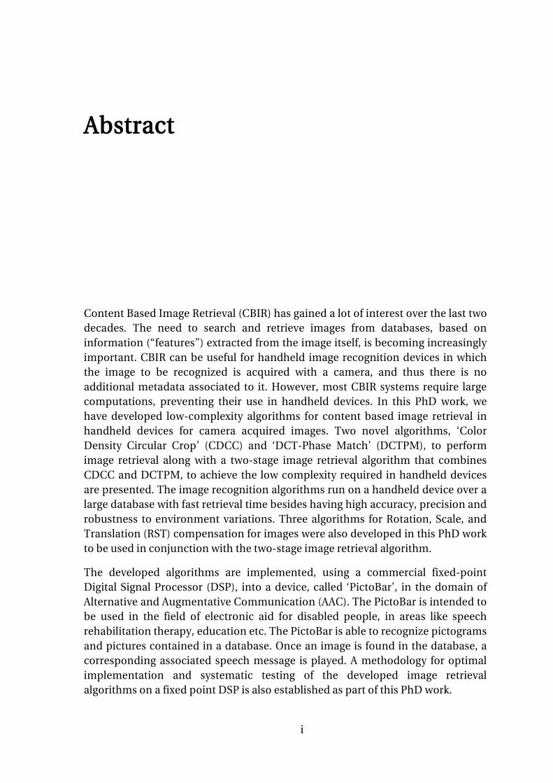
Abstract

Content Based Image Retrieval (CBIR) has gained a lot of interest over the last two decades. The need to search and retrieve images from databases, based on information (“features”) extracted from the image itself, is becoming increasingly important. CBIR can be useful for handheld image recognition devices in which the image to be recognized is acquired with a camera, and thus there is no additional metadata associated to it. However, most CBIR systems require large computations, preventing their use in handheld devices. In this PhD work, we have developed low-complexity algorithms for content based image retrieval in handheld devices for camera acquired images. Two novel algorithms, ‘Color Density Circular Crop’ (CDCC) and ‘DCT-Phase Match’ (DCTPM), to perform image retrieval along with a two-stage image retrieval algorithm that combines CDCC and DCTPM, to achieve the low complexity required in handheld devices are presented. The image recognition algorithms run on a handheld device over a large database with fast retrieval time besides having high accuracy, precision and robustness to environment variations. Three algorithms for Rotation, Scale, and Translation (RST) compensation for images were also developed in this PhD work to be used in conjunction with the two-stage image retrieval algorithm.

The developed algorithms are implemented, using a commercial fixed-point Digital Signal Processor (DSP), into a device, called ‘PictoBar’, in the domain of Alternative and Augmentative Communication (AAC). The PictoBar is intended to be used in the field of electronic aid for disabled people, in areas like speech rehabilitation therapy, education etc. The PictoBar is able to recognize pictograms and pictures contained in a database. Once an image is found in the database, a corresponding associated speech message is played. A methodology for optimal implementation and systematic testing of the developed image retrieval algorithms on a fixed point DSP is also established as part of this PhD work.

ii

Keywords: low-complexity, image recognition, content based image retrieval, alternative and augmentative communication, RST compensation, handheld image recognition device, color density circular crop, DCT-phase match, two-stage image retrieval, Fourier-Mellin transform, Hough transform, Harris corner detector, perspective transform, DSP implementation, codec-engine, PictoBar.

iii

Résumé

Au cours des deux dernières décennies, la recherche d’images par le contenu (en anglais Content Based Image Retrieval ou CBIR) a suscité un intérêt de plus en plus vif. La nécessité de rechercher et récupérer des images dans des bases de données, en utilisant comme critère des informations (« caractéristiques ») extraites de l’image elle-même, devient de plus en plus importante. Ce type de recherche peut être utile pour la reconnaissance d’images sur un appareil portable, où l’image à reconnaître est capturée par une caméra, et est donc dépourvue de métadonnées additionnelles. Cependant, la plupart des systèmes de ce genre requièrent un nombre important de calculs, ce qui empêche leur utilisation sur des dispositifs portables. Dans ce travail de thèse, nous avons développé des algorithmes à faible complexité pour la recherche d’images par le contenu sur des appareils portables qui permettent la capture d’images via une caméra. Deux algorithmes originaux, Color Density Circular Crop (CDCC) et DCT-phase match (DCTPM), sont présentés pour effectuer la recherche d’images, ainsi qu’un algorithme de recherche d’images à deux étapes qui combine CDCC et DCTPM, de manière à atteindre la faible complexité requise sur un appareil portable. Les algorithmes de reconnaissance d’images sont exécutés sur un appareil portable doté d’une base de données importante. Ils permettent des recherches rapides, qui sont également exactes, à haute précision, et résistantes aux variations de l’environnement. Trois algorithmes visant à compenser la rotation, le changement d’échelle, et la translation des images ont également été développés dans ce travail de thèse, pour être utilisés en conjonction avec l’algorithme de recherche d’images à deux étapes.

Les algorithmes développés ont été implémentés sur un DSP commercial à virgule fixe embarqué dans un appareil appelé « PictoBar », dont le champ d’application est la Communication Améliorée et Alternative (CAA). PictoBar est destiné à être utilisé dans le domaine de l’assistance électronique aux personnes

iv

handicapées, pour les thérapies de réadaptation de la parole, l’éducation, etc. PictoBar est capable de reconnaître des pictogrammes et des photographies contenues dans une base de données. Lorsqu’une image est identifiée dans la base de données, le message vocal associé correspondant est reproduit. Une méthodologie d’implémentation optimale et de test systématique des algorithmes de recherche d’images proposés sur un DSP à virgule fixe a également été établie au cours de ce travail de thèse.

Mots-clés : faible complexité ; reconnaissance d’images ; recherche d’images par le contenu ; communication améliorée et alternative ; compensation de rotation, de changement d’échelle et de translation ; reconnaissance d’images sur appareil portable ; CDCC ; DCTPM ; recherche d’images à deux étapes ; transformée de Fourier-Mellin ; transformée de Hough ; transformée de Harris ; détecteur de coins de Harris ; transformation de perspective ; implémentation sur DSP ; codec-engine ; Pictobar.

v

Acknowledgements

This work could not have been accomplished without the support of many colleagues, staff, friends and family that I would like to thank. I would first like to thank Prof. Dr. Pierre-André Farine for giving me the opportunity to pursue this research in ESPLAB and for his support over the last four years.

I am particularly grateful to my advisor Dr. Sara Grassi Pauletti for her guidance and support during the entire PhD work. Moreover she provided great assistance in the course of writing this document. It has been a great pleasure working under her guidance. At the same time, I would like to express my gratitude to the jury members of my thesis committee, Prof. Dr. Hans Peter Herzig, Prof. Dr. Michaël Unser, Prof. Dr. Roger Gassert, and Dr. Robert Van Kommer for investing their time to proofread my thesis and evaluate this work. I also would like to thank Dr. Javier Bracamonte for his initial support as my advisor when I started my PhD.

I would like to thank the Swiss Federal Office for Professional Education and Technology (OPET) through the Innovation Promotion Agency (CTI) for the funding during the PhD work, under the Grant CTI 8811.2 PFNM-NM ("PictoBar" project). I am also grateful for our project partners Nicolas Deurin and Thierry Gueguen from Epicard SA; Michel Guinand , Christian Vaucher, Yves Mühlebach and Yvan Magnin from FST; Timothée Carron, Yvan Favre and Julien Tharin from Gigatec SA, for their fruitful collaboration during the project. I also like to thank the students from EPFL who worked with me on different semester projects and in particular Mr. Pascal Bach and Mr. Axel Perruchoud.

I would like to thank Dr. Patrick Stadelmann, who translated the abstract of the thesis into French, and Dr. Urs Alexander Müller, for proofreading chapter 3 of this document. I also would like to thank my very good friend Neeraj Adsul for his valuable time to proofread this document and his valuable comments.

vi

I am really grateful to all my colleagues and friends at ESPLAB for the wonderful time over the last four years and in particular to Mohssen Moridi, Aleksandar Jovanovic, Youssef Tawk, Mitko Tanevski, Yazhou Zhao, Christian Robert, Chao Wang, Saeed Ghamari, Ban Wang, Marcel Baracchi-Frei, Grégoire Waelchli, Kilian Imfeld, Luca Rossi, Laurent Ferrari, Ali Shafqat, Nastaran Asadi Zanjani, Shiv Ashish Kumar, Biswajit Mishra, Hind Meyer, Jaskaranjeet Singh, Marko Stojanovic, Miguel Angel Ribot Sanfelix, Steve Tanner, Cyril Botteron, Gabriele Tasselli, Mirjana Banjevic, Phillip Tomé, Amadou Hadji, Enrique Rivera, Jaleed Khawaja and Marco Marassi.

I also would like to thank all those who are responsible for the administrative work. I am particularly thankful to Joëlle Banjac, Florence Rohrbach, Marie Halm, Sandra Roux and Sandrine Piffaretti.

I also would like to thank my friends outside EPFL who made sure the life outside work was equally memorable. In particular I would like to thank Ashutosh Ghildiyal, Neetha Ramanan, Sri Harsha Kasi Raj, Devulapalli Chakravarty, Prakash Thoppay, Arun Mohan, Reshma Sahasrabudhe, Anu Arun, Gurpreet Kaur Gulati, Ritayan Roy, Thejesh Bandi, Paul Baillieux, Heidi Guzman Graf, Shanmugabalaji Venkatasalam, Justin Paulraj John Peter, Ashok Munusamy Lakshmanan, Rajan Thambehalli, Dipti Abhilasha and Mira Eileen Burmeister Rudolph.

Finally, I would like to thank my entire family and in particular my grandparents Shakuntala Ayyalasomayajula and Narasimha Murty Ayyalasomayajula, and Varalaxmi Ganti and Venkat Rao Ganti; my uncle Dr. Ratna Phani Ayalasomayajula and my aunt Anu Radha Ayalasomayajula. A special thanks to my sister, Gita Rani Ayyalasomayajula, who always had the patience and time to listen to my stories. Last but not the least, for their unconditional love, care, and support that I receive; I would like to specially thank my parents Padmavathi Ayyalasomayajula and Venkata Chenulu Ayyalasomayajula, for whom my life is indebted.

vii

Abbreviations

AAC Alternative and Augmentative Communication

AIC Audio Integrated Circuit

ALU Arithmetic Logic Unit

API Application Programming Interface

ARM Advanced RISC Machines

ASCII American Standard Code for Information Interchange

ASP Audio Serial Port

BM Best Match

BoW Bag of Words

BRRP Border Recognition, Reconstruction and Preprocessing

CBIR Content Based Image Retrieval

CCS Code Composer Studio

CDCC Color Density Circular Crop

CE Codec Engine

CMEM Contiguous Memory

DCT Discrete Cosine Transform

DCTPM Discrete Cosine Transform Phase Match

viii

DDR Double Data Rate

DFT Discrete Fourier Transform

DM Digital Media

DMA Direct memory access

DoG Difference of Gaussians

DSP Digital Signal Processor

EMD Earth Mover's Distance

EMIF External Memory Interface

EPFL École Polytechnique Fédérale de Lausanne

ESPLAB Electronics and Signal Processing Laboratory

FC Framework Components

FFT Fast Fourier Transform

FMT Fourier-Mellin Transform

FST La Fondation Suisse pour les Téléthèses

FT Fourier Transform

GUI Graphical User Interface

HLOS High Level Operating Systems

HOG Histogram of Oriented Gradients

I2C Inter-Integrated Circuit

IC Integrated Circuit

IP Internet Protocol

JPEG Joint Photographic Experts Group

JTAG Joint Test Action Group

K-L Kullback-Leibler

LED Light Emitting Diode

MAC Multiply And Accumulate

MATLAB MATrix LABoratory

ix

MFP Multimedia Framework Products

MIPS Million Instructions Per Second

MMACs Million MACs per Second

MMC Multimedia Card

MMU Memory Management Unit

MPEG Moving Picture Experts Group

MT Mellin transform

NFS Network File System

NTSC National Television Standards Committee

OS Operating System

PAL Phase Alternating Line

PCA Principal Component Analysis

PCS Picture Communication Symbols

PhD Philosophiae Doctor

PSP Processor Support Package

QBE Query By Example

QVGA Quarter-Video Graphics Array

RGB Red, Green, Blue

RISC Reduced Instruction Set Computer

RM Region Merging

RMAN Resource Manager

RST Rotation, Scaling and Translation

RTOS Real-Time Operating System

RTSC Real-Time Software Components

SBM Second Best Match

SD Secure Digital

SDK Software Development Kit

x

SDRAM Synchronous Dynamic Random Access Memory

SECAM Sequentiel Couleur Avec Mémoire

SIFT Scale Invariant Feature Transform

SoC System on Chip

SSH Secure Shell

SURF Speeded Up Robust Features

SUSAN Smallest Univalue Segment Assimilating Nucleus

SVM Support Vector Machine

TI Texas Instruments

USAN Univalue Segment Assimilating Nucleus

USB Universal Serial Bus

VGA Video Graphics Array

VICP Video Imaging Co-Processor

VISA Video, Imaging, Speech and Audio

VLIB Video Analytics & Vision Library

VLIW Very Long Instruction Word

VPBE Video Processing Back-End

VPFE Video Processing Front-End

VPSS Video Processing Subsystem

XDAIS eXpressDSP Algorithm Interoperability Standard

xDM eXpressDSP Digital Media

YCbCr Luminance; Chroma: Blue; Chroma: Red

Contents

Abstract........................................................................................................................... i

Résumé ......................................................................................................................... iii

Acknowledgements ...................................................................................................... v

Abbreviations .............................................................................................................. vii

1. Introduction .............................................................................................................. 1

1.1. Motivation ......................................................................................... 2

1.2. Scope of the PhD work ..................................................................... 4

1.3. Objectives and outline of the PhD work ......................................... 5

1.4. Main scientific contributions .......................................................... 6

1.5. Publications ...................................................................................... 7

2. Content based image retrieval ................................................................................. 9

1 Content Based Image Retrieval ........................................................................... 10

1.1. Introduction .................................................................................... 10

1.2. Image features ................................................................................ 12

1.3. Similarity measure .......................................................................... 12

2 CBIR algorithms ................................................................................................... 14

2.1. Color histograms ............................................................................ 14

2.2. Color moments and moment invariants ...................................... 17

2.3. Scale Invariant Feature Transform................................................ 19

2.4. Histogram of Oriented Gradients .................................................. 21

2.5. GIST feature descriptor .................................................................. 22

2.6. Bag of Words (BoW)........................................................................ 23

2.7. Other methods ................................................................................ 24

2.7.1. Shape aware methods ................................................................. 24

2.7.2. Speeded Up Robust Features ..................................................... 24

2.7.3. Textons ........................................................................................ 25

2.7.4. Machine learning methods ........................................................ 25

3 Conclusions and summary of the chapter ..................................................... 25

3. Image retrieval algorithms ..................................................................................... 27

1 Color Density Circular Crop ................................................................................ 28

1.1. Introduction .................................................................................... 28

1.1.1. Color fundamentals .................................................................... 28

1.1.2. Color spaces ................................................................................ 29

RGB color model ...................................................................... 29

YUV color model ...................................................................... 30

YCbCr color model ................................................................... 31

1.2. CDCC algorithm ............................................................................. 31

1.2.1. Feature extraction ....................................................................... 32

Circular segmentation ............................................................. 32

Concentric Circular Crop ........................................................ 33

Color Density calculation ........................................................ 33

Color Density normalization ................................................... 33

1.2.2. Similarity calculation and image retrieval ................................ 34

1.3. Experimental evaluation ................................................................ 35

1.3.1. Experimental databases ............................................................. 35

1.3.2. Testing procedure ....................................................................... 35

1.3.3. Results .......................................................................................... 36

2 DCT-phase match ................................................................................................ 38

2.1. Introduction .................................................................................... 38

2.1.1. Discrete Cosine Transform......................................................... 38

2.1.2. JPEG compression ....................................................................... 40

2.2. DCTPM algorithm .......................................................................... 42

2.2.1. DCT-phase for image retrieval ................................................... 42

DCT-phase of an image ........................................................................... 42

DCT-phase representation ..................................................................... 43

2.2.2. Retrieval algorithm for occluded images .................................. 44

Correlation metric ................................................................................... 44

Region merging ........................................................................................ 45


2.3.1. Experimental database ............................................................... 46

2.3.2. Testing procedure and results .................................................... 47

3 Low complexity image retrieval algorithm ........................................................ 51

3.1. Introduction .................................................................................... 51

Two-stage search ..................................................................... 51

3.2. Proposed image retrieval algorithm .............................................. 51

3.2.1. Border Recognition, Reconstruction and Preprocessing (BRRP) ...................................................................................................... 51

3.2.2. Color Density Circular Crop (CDCC) Pre-selection.................. 51

3.2.3. DCT Phase Match (DCTPM) ...................................................... 52


3.3.1. Experimental database ............................................................... 53

Camera Setup ............................................................................... 53

3.3.2. Testing procedure and results .................................................... 54

3.3.3. Comparison with other retrieval algorithms ............................ 57


4. Rotation, scaling, and translation compensation algorithms ............................. 61

1 Introduction ......................................................................................................... 62

1.1. Mathematical representation of rotation, scaling and translation . ......................................................................................................... 62

Rotation .................................................................................... 62

Scaling ....................................................................................... 63

Translation ............................................................................... 63

RST transform representation ................................................. 63

2 RST compensation without printed reference................................................... 64

2.1. Fourier-Mellin transform ............................................................... 64

2.2. Implementation of Fourier-Mellin transform .............................. 65

2.2.1. Log-polar grid interpolation....................................................... 66


2.3.1. Test databases ............................................................................. 68


2.3.3. Test results ................................................................................... 70

3 RST compensation with printed reference ........................................................ 70

3.1. Line detection ................................................................................. 71

3.1.1. Hough transform......................................................................... 72

3.1.2. Implementation of Hough transform for rectangle detection 72

3.2. Corner detection ............................................................................. 73

3.2.1. Harris corner detector [83] ......................................................... 74

3.2.2. Smallest Univalue Segment Assimilating Nucleus (SUSAN) ... 76

3.2.3. Implementation of rectangle detection based on Harris corner detector and modified SUSAN ........................................................................... 77

3.3. Perspective transform for RST compensation.............................. 78

3.3.1. Implementation of RST compensation ..................................... 80


3.4.1. Test databases ............................................................................. 81


3.4.3. Test results ................................................................................... 82


5. DSP implementation of the image recognition algorithm and application in a handheld device for alternative and augmentative communication ..................... 85

1 Introduction ......................................................................................................... 86

2 The PictoBar device ............................................................................................. 86

2.1. Device hardware ............................................................................. 87

2.2. Device specifications ...................................................................... 88

2.3. Use of PictoBar ............................................................................... 89

3 Image recognition algorithm .............................................................................. 89

3.1. Border Recognition, Reconstruction and Preprocessing (BRRP) 89

3.2. Color Density Circular Crop (CDCC) ............................................ 90

3.3. DCT Phase Match (DCTPM) .......................................................... 91

3.4. Camera setup and calibration ....................................................... 91

3.5. Databases ........................................................................................ 92

3.6. MATLAB demonstrator .................................................................. 93

4 DSP implementation ........................................................................................... 94

4.1. TMS320DM6446 ............................................................................. 94

4.2. Software framework ....................................................................... 95

4.2.1. xDAIS and xDM ........................................................................... 96

4.2.2. HLOS: Linux Utils and WinCE Utils ........................................... 96

4.2.3. Framework Components............................................................ 96

4.2.4. Codec Engine framework ........................................................... 96

4.3. Development environment ........................................................... 97

4.4. ARM application ............................................................................. 98

4.5. Libraries .......................................................................................... 99

4.6. CODECS ........................................................................................ 100

4.6.1. BRRP .......................................................................................... 100

4.6.2. CDCC ......................................................................................... 101

4.6.3. DCTPM ...................................................................................... 101

4.6.4. JPEG decoder ............................................................................. 102

4.7. Testing ........................................................................................... 102

4.8. Results ........................................................................................... 102

5 Conclusions and summary of the chapter ....................................................... 103

6. Conclusion ............................................................................................................ 105

1 Summary and recall of the contributions ........................................................ 106

2 Discussions and future work ............................................................................ 107

References ................................................................................................................. 109

Chapter 1

Introduction

In this chapter, an introduction and motivation to the research carried out in this PhD work is presented along with the scope of the research and main scientific contributions of the PhD work. The chapter is organized as follows: In subsection 1, the motivation for the research is introduced followed by the scope of the research in subsection 2. In subsection 3, objectives and outline of the PhD work are discussed. In subsection 4, the main scientific contributions of the PhD work are discussed followed by the scientific publications produced as part of this PhD work in subsection 5.

Chapter 1 2

1.1. Motivation

Humans are not just biological creatures; we are social animals, the most social on earth. The term ‘social’ refers to our ability to form recognizable and distinct societies. Humans did not become social animals in a day from Athena, the Greek goddess of wisdom; rather they evolved and developed into social animals over tens of thousands of years. The quintessential part of this evolution is the ability to communicate with other members of the species by using both verbal and non-verbal messages. One of the important non-verbal communication is pictures, as rightly described in a Chinese proverb - “A picture is worth a thousand words”.

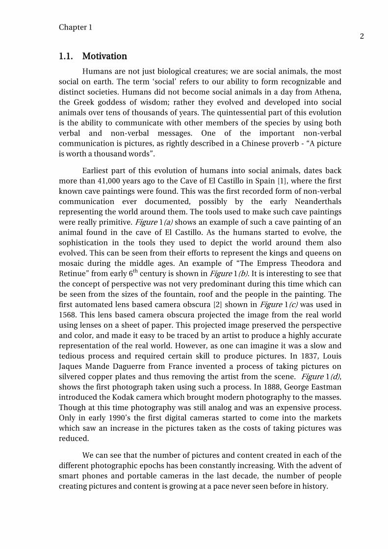
Earliest part of this evolution of humans into social animals, dates back more than 41,000 years ago to the Cave of El Castillo in Spain [1], where the first known cave paintings were found. This was the first recorded form of non-verbal communication ever documented, possibly by the early Neanderthals representing the world around them. The tools used to make such cave paintings were really primitive. Figure 1(a) shows an example of such a cave painting of an animal found in the cave of El Castillo. As the humans started to evolve, the sophistication in the tools they used to depict the world around them also evolved. This can be seen from their efforts to represent the kings and queens on mosaic during the middle ages. An example of “The Empress Theodora and Retinue” from early 6th century is shown in Figure 1(b). It is interesting to see that the concept of perspective was not very predominant during this time which can be seen from the sizes of the fountain, roof and the people in the painting. The first automated lens based camera obscura [2] shown in Figure 1(c) was used in 1568. This lens based camera obscura projected the image from the real world using lenses on a sheet of paper. This projected image preserved the perspective and color, and made it easy to be traced by an artist to produce a highly accurate representation of the real world. However, as one can imagine it was a slow and tedious process and required certain skill to produce pictures. In 1837, Louis Jaques Mande Daguerre from France invented a process of taking pictures on silvered copper plates and thus removing the artist from the scene. Figure 1(d), shows the first photograph taken using such a process. In 1888, George Eastman introduced the Kodak camera which brought modern photography to the masses. Though at this time photography was still analog and was an expensive process. Only in early 1990’s the first digital cameras started to come into the markets which saw an increase in the pictures taken as the costs of taking pictures was reduced.

We can see that the number of pictures and content created in each of the different photographic epochs has been constantly increasing. With the advent of smart phones and portable cameras in the last decade, the number of people creating pictures and content is growing at a pace never seen before in history.

Chapter 1 3

The majority of the content created in the last couple of decades is in digital format; this has motivated researchers in the digital image processing domain to tackle challenges such as digital image analysis, restoration, recognition, indexing and organization. Among them, Content Based Image Retrieval (CBIR) has gained lot of interest from researchers starting from the early 1990’s. CBIR uses visual contents or information extracted from the image, to describe the image and to search for its closest match within a database of possible images. CBIR is different from retrieval approach based on attaching textual metadata to each image and use traditional database query techniques to retrieve images by keywords, tags, and/or descriptions associated with the image. CBIR has been used in several applications such as fingerprint identification, image matching, digital libraries, medicine, crime prevention, historical research, among others.

New applications of CBIR using handheld devices are becoming increasingly popular. There are many commercially available apps on smart

(a) (b)

(c) (d)

Figure 1: (a) Cave painting found in the cave of El Castillo, (b) Mosaic depicting ‘The Empress Theodora and Retinue’ from 6th century, (c) First automated lens based camera obscura, (d) ‘Still Life’, the first photograph taken on silvered copper plate.

Chapter 1 4

phones like Google Goggles, Snaptell and LookTel which use some concepts of CBIR. Most of these apps use algorithms which are highly computationally complex and typically use servers hosted on the internet to perform required computations for finding the exact match.

For a fairly large database, it is still a challenge to perform image matching and retrieval, locally on a handheld device, without the support of external computational units. To overcome this challenge, we need to develop new algorithms meeting the following four general specifications:

• Low complexity –for low power implementation which is critical in handheld devices

• Fast retrieval –for effective operation by a user • High accuracy and precision –for retrieval of the best match as the query

image in most of the cases • Robustness –for reliability across variations in the environment and practical

usage

In this PhD work we explore the area of Content Based Image Retrieval (CBIR) for portable and handheld devices and present algorithms taking into considerations the above broad specifications. There are many applications for such a handheld CBIR device. One such application is in the field of electronic aid for disabled people which has been growing constantly with many innovations being added every year. The need for electronic aids in Alternative and Augmentative Communication (AAC) is becoming increasingly important and next generation devices in AAC will very likely integrate a camera and image processing capabilities along with other traditional features.

1.2. Scope of the PhD work

The research presented in this PhD work is in the domain of image processing and is limited to the area of content based image retrieval. In particular the study was restricted to retrieval of images for portable and handheld devices. Also the retrieval algorithms were designed and tested for two distinct datasets namely; a dataset of natural images also referred to as ‘pictures’ (images which have a rich local covariance structure), and a dataset of pictograms (images which have limited colors and convey a meaning through pictorial representation of a physical object or an action). In this document, the terms “pictures” and “pictograms” are used to differentiate one dataset from another; the term “images” is used for both in a general sense.

The research presented in this document has both an algorithmic development part and its implementation on a commercial Digital Signal Processor (DSP) from Texas Instruments (TMS320DM6446). All the algorithms

Chapter 1 5

developed as part of this PhD work were low complexity algorithms, optimized for handheld devices and DSP implementation.

The research deals with one to one exact matching of query image with images in a database and does not deal with other CBIR areas like image/object classification, learning methods etc. It is important to differentiate between image recognition and image retrieval which is very subtle. Image recognition refers to whether or not the image data contains some specific object, feature, or activity. Image retrieval refers to finding all images in a larger set of images which have a specific content. Videlicet, image recognition is a super set which includes image retrieval as one of its important subsets along with other subsets like detection and identification of useful content in the image which can be used by image retrieval etc. In this PhD work we use image recognition to refer to the complete algorithm, which takes in an image from the camera as a query and gives the best match as the output, and image retrieval for the individual blocks of the recognition algorithm which perform matching.

1.3. Objectives and outline of the PhD work

The PhD work has two major objectives. The first objective is to develop image recognition algorithms for handheld devices. The recognition algorithms have to be low in complexity such that they can run locally on a portable handheld device for camera acquired images. The algorithms should also be Rotation, Scaling, and Translation (RST) invariant for practical handheld usage.

The second objective of the PhD work is to implement the developed image recognition algorithms for application in Alternative and Augmentative Communication (AAC). The implemented algorithms have to be able to recognize pictograms and pictures contained in a database and once the image is found in the database, a corresponding associated speech message should be played. The recognition algorithms have to be ported to a dual core device (TMS320DM6446) which contains a fixed point DSP. This application had several constrains on the database size, recognition time etc. For example, the recognition algorithms have to be fast enough such that the recognition time is less than one second and a typical database would contain around 1000 to 5000 pictograms and pictures. Such a device is intended to be used by language re-education professionals and specialized educators in the treatment of people affected by pathologies such as aphasia, autism, trisomy or mental handicaps.

This PhD work is organized into six chapters. In the first chapter, the introduction and motivation to the research carried out is presented along with the scope of the research and main scientific contributions of the research.

Chapter 1 6

In the second chapter, the introduction to the content based image retrieval is presented. This is followed by a brief introduction to current state of the art CBIR methods.

In the third chapter, the two developed image retrieval algorithms, ‘Color Density Circular Crop’ (CDCC) and ‘DCT-phase match’ (DCTPM), are explained. This is followed by a low complexity image retrieval algorithm which combines these two algorithms, performing image retrieval in two stages.

In the fourth chapter, algorithms for rotation, scaling, and translation compensation are presented. Three different RST compensation algorithms are presented in this chapter. The first algorithm uses Fourier-Mellin Transform to perform RST compensation and does not use any printed reference on the image. The second and third algorithms use a rectangular border as a printed reference around the image to perform RST compensation.

An application of the above mentioned algorithms for an Alternative and Augmentative Communication (AAC) device is presented in the fifth chapter. The implementation of the proposed algorithms for this application on a fixed point DSP (TMS320DM6446) is also presented in this chapter.

In the sixth chapter, the conclusions of the PhD work and future work are discussed.

1.4. Main scientific contributions

The main scientific contributions of the PhD work described in this document are:

(1) A two-stage low-complexity image retrieval algorithm for handheld devices which is presented in chapter 3. For the first stage we have developed an algorithm called “Color Density Circular Crop” (CDCC) which uses color content of the images to perform matching. For the second stage, we have developed an algorithm called “Discrete Cosine Transform Phase Match” (DCTPM) which uses spatial features in the images to perform matching.

(2) Three algorithms for Rotation, Scaling, and Translation (RST) compensation for images are presented in chapter 4. The first RST compensation algorithm is based on Fourier-Mellin Transform (FMT) and uses no printed reference on the image. The second and thrid RST compensation algorithm uses a rectangle as a printed reference which is detected by Hough transform and corner detection.

(3) A methodology for optimal implementation of the above algorithms on a fixed point DSP which is presented in chapter 5.

Chapter 1 7

1.5. Publications

Part of the work described in this document has already been subject to some publications.

The first stage of the algorithm which is used as pre-selection algorithm has been presented at the Seventh International Symposium on Image and Signal Processing and Analysis (ISPA’11) in Croatia, in September 2011[3]. The second stage of the algorithm, used to perform image retrieval is presented at the Nineteenth IEEE International Conference on Image Processing (ICIP’12) in USA, in September 2012 [4]. These two algorithms are explained in more detail in chapter 3 of the document.

A paper on low-complexity RST compensation algorithm, without using any printed reference on the image, was presented at the Nineteenth European Signal Processing Conference (EUSIPCO’11) in Spain, in August 2011 [5]. This is discussed in more detail in chapter 4 along with the image RST compensation algorithms with printed references on the image.

In the paper at the Seventh Conference on Ph.D. Research in Microelectronics and Electronics (PRIME’11) in Italy, in July 2011 [6], we presented an application of the CBIR algorithm for an AAC device. The paper presented at the Fourth European DSP in Education and Research Conference (EDERC’10) in France, in December 2010 [7], describes the implementation of the proposed low-complexity algorithms on a commercial DSP. The application of the CBIR algorithms and its DSP implementation is discussed in more detail in chapter 5 of the document.

Chapter 2

Content based image retrieval

In this chapter, an introduction to Content Based Image Retrieval (CBIR) is presented and different seminal algorithms for content based image retrieval which are used in the field are reviewed. The chapter is organized as follows: In section 1, content based image retrieval and its constitutive blocks are introduced. In section 2, different content based image retrieval algorithms and methods which are currently used in the field are reviewed.

Chapter 2 10

1 Content Based Image Retrieval

1.1. Introduction

Content Based Image Retrieval (CBIR) has been around for more than two decades. The term CBIR seems to have originated in 1992, when it was used by T. Kato [8] to describe experiments about automatic retrieval of images from a database, based on the colors and shapes present in the images. The term has since been widely used to describe the process of retrieving desired images from a large collection, on the basis of features (such as color, texture, and shape) that can be extracted from the images themselves. The features used for retrieval can be either primitive (such as edges, corners, change in direction etc.) or semantic (such as objects, faces, etc.) but the extraction process must be predominantly automatic.

CBIR differs from classical information retrieval in a way that image databases are essentially unstructured, i.e., digitized images consist of arrays of pixel intensities, with no inherent meaning. One of the key issues with any sort of image processing is the need to extract useful information from the raw data (such as recognizing the presence of particular shapes) before reasoning about the image’s contents. Image databases thus differ fundamentally from text databases, where the input such as words, comprising of ASCII characters, is inherently been logically structured [9]. Retrieval of images by manually assigned keywords is not CBIR as the term is generally understood, even if the keywords describe image content.

There exist many CBIR query modalities. ‘Query By Example’ (QBE) is a query modality that involves providing a CBIR system with an example image as the input for search. The underlying search algorithms may vary depending on the application, but resulting images should all share common elements with the provided example (input) image. This query modality removes the difficulties that can arise when trying to describe images with words. ‘Semantic retrieval’ is where the user makes a query based on words which might describe the image, like "find pictures of Albert Einstein". This type of open-ended task is difficult to perform as Einstein may not always be facing the camera or having the same pose. Therefore, current CBIR systems generally make use of lower-level features like texture, color, and shape, although some systems take advantage of common higher-level features like faces for semantic retrieval. Other query modalities include navigating customized/hierarchical categories [10], querying by image region rather than the entire image [11], querying by multiple example images [12], querying by visual sketch where a rough approximate drawing of the image is provided by the user like blobs of color or general shapes [13], querying by direct specification of image features, and multimodal queries [14] (e.g. combining touch, voice, etc.). CBIR systems can also make use of relevance feedback, where

Chapter 2 11

the user progressively refines the search results by marking the images in the results as "relevant", "not relevant" or "neutral" to the search query, then repeating the search with the new information [15]. It should be noted that not every CBIR system is generic and most systems are designed for a specific domain. Henceforth when we refer to a CBIR system we confine ourselves to ‘Query by example’ modality in this document.

The applications of CBIR span oven many areas like alternative and augmentative communication, education and training, architectural and engineering design, intellectual property, military, medical diagnosis, journalism and advertising, and home entertainment to name a few. The impact of CBIR has been steadily increasing with many new application areas being added every day. While the problems of image retrieval in a general context have not yet been satisfactorily solved, by exploiting natural constraints and by working within restricted domains the problem of image retrieval is currently resolved.

Any CBIR system has two main stages at its core. Videlicet, feature extraction and similarity measure. This is followed by ranking of images based on the similarity measure. A general block diagram of a CBIR system is shown in Figure 2. This includes two sections, one performed offline, where the image features are pre-extracted from an image database on which retrieval has to be performed and stored as an image feature database, and the other online, where an image query is presented to the CBIR system and we compute the features of this image query and compare it with the pre-computed image features database and rank the results to retrieve the closest matching images.

Figure 2: Block diagram showing an overview of content based image retrieval system using ‘query by example’ modality.

Chapter 2 12

In the next subsections we see in more detail the key individual blocks of a CBIR system.

1.2. Image features

A feature is a numerical representation which captures a certain visual property of an image, either globally for the entire image or locally for a small group of pixels. The most commonly used features include those reflecting color, texture, shape, and salient points in an image. In global extraction, features are computed to capture the overall characteristics of an image. The advantage of global extraction is its high speed for both extracting features and computing similarity. However, global features are often too rigid to represent an image. Specifically, they can be oversensitive to location and hence fail to identify important visual characteristics. To increase the robustness to spatial transformation, the second approach to compute features is by local extraction. In local feature extraction, a set of features are computed for every pixel using its neighborhood pixels. To reduce computation, an image may be divided into small, non-overlapping blocks, and features are computed individually for every block. The features are still local because of the small block size, but the amount of computation is only a fraction of that for obtaining features around every pixel.

The features, apart from capturing the essence of an object, should be invariant to changes such as lighting, viewpoint, rotation, scaling etc. Here, we define invariance of a feature to condition A as: the feature is independent and unaffected by any changes in condition A.

A feature descriptor, sometimes referred to as “image signatures” or just “descriptor”, is a set of features which can be used to discriminate one image from another. An abstract space in which each feature descriptor is represented as a point in n-dimensional space is called the feature space. Feature descriptors can generally be dichotomized into fixed length descriptors and adaptive length descriptors. The fixed length descriptors usually consist of either vectors or distributions. Adaptive length descriptors generally use learning methods that are used to tune signatures based on the input.

1.3. Similarity measure

The concept of similarity is fundamentally important in almost every scientific field. Similarity measure is used to represent how similar or close are two feature descriptors in the feature space. Similarity (or more accurately dissimilarity) is often characterized as a distance in some suitable feature space that is assumed to be a metric space. To measure this distance 𝐿𝑝-norm or p-norm is often used. Some of the frequently used similarity measures in CBIR are presented below.

Chapter 2 13

Manhattan distance metric, also known as city block distance or taxicab distance, is widely used in CBIR to compute similarity distance between two feature descriptors. Manhattan distance is a distance measure in 𝐿1 space and is defined as:

�|𝑥𝑖 − 𝑦𝑖|𝑛

𝑖=1

(1)

The most commonly used distance similarity metric is the Euclidean distance. The Euclidean distance metric between two feature descriptors 𝐴 = (𝑥1,𝑥2, 𝑥3, … , 𝑥𝑛) and 𝐵 = (𝑦1,𝑦2, 𝑦3, … ,𝑦𝑛) ∈ ℝ𝑛 can be considered as a distance measure in 𝐿2 space and is defined as:

��|𝑥𝑖 − 𝑦𝑖|2𝑛

𝑖=1

� (2)

The Minkowski distance is a metric on 𝐿𝑝 space which can be considered as a generalization of both the Euclidean distance and the Manhattan distance. The Minkowski distance of order p between two points 𝐴 = (𝑥1, 𝑥2, 𝑥3, … , 𝑥𝑛) and 𝐵 = (𝑦1,𝑦2,𝑦3, … , 𝑦𝑛) ∈ ℝ𝑛 is defined as:

��|𝑥𝑖 − 𝑦𝑖|𝑝𝑛

𝑖=1

�

1𝑝

(3)

In the limiting case of 𝑝 reaching infinity the Minkowski distance becomes the Chebyshev distance, which gives the distance between two points in n-dimensional vector space in the 𝐿∞ space. The Chebyshev distance is also called as chessboard distance, since in the game of chess the minimum number of moves needed by a king to go from one square on a chessboard to another equals the Chebyshev distance between the centers of the squares. The Chebyshev distance is defined as:

lim𝑝→+∞

��|𝑥𝑖 − 𝑦𝑖|𝑝𝑛

𝑖=1

�

1𝑝

= max𝑖=1𝑛 |𝑥𝑖 − 𝑦𝑖| (4)

There exist many similarity measures beyond the ones mentioned above [16] which are used in CBIR. In particular the class of similarly measures that are based on different probability models [17-19] has been widely used in recent times.

Chapter 2 14

2 CBIR algorithms

In this section we present different CBIR algorithms which had seminal impact on the field of content based image retrieval. The algorithms and methods presented here are not meant to be exhaustive, but are chosen to describe different approaches used in the field for image retrieval.

2.1. Color histograms

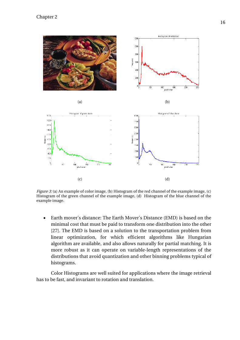
A color histogram is obtained by discretizing the colors present in an image and counting the number of times each discrete color occurs in the image. The use of color histograms in image retrieval was first introduced by Swain and Ballard [20]. Histograms by their nature, are invariant to translation and rotation, and change slowly under change of angle of view, change in scale and occlusion. Many color histogram models which take histograms over different channels in different color spaces [21] are used in image retrieval. An example of color histograms on the RGB color channels of an image is shown in Figure 3. Histograms are currently used in many applications where speed and low complexity are predominant.

The color histograms can be summarized to three categories, by considering integrating over some of the data dimensions. Videlicet, global image histograms – are obtained by integration over the spatial coordinates and all the spatial information present in the image is lost [20]; Horizontal/Vertical projections – only one of the spatial coordinates is integrated over [22]; and Multiple region histograms – histograms are computed over different regions in the image [23].

Several measures have been proposed for the similarity between two histograms. We divide them into two categories. The bin-by-bin similarity measures only compare contents of corresponding histogram bins, that is, they compare 𝑃𝑖 and 𝑄𝑖 for all 𝑖, but not 𝑃𝑖 and 𝑄𝑗 for 𝑖 ≠ 𝑗, where 𝑃,𝑄, represent the

binned distributions and the subscripts 𝑖, 𝑗 represent the bins. The cross-bin measures also contain terms that compare non-corresponding bins. Predictably, bin-by-bin measures are more sensitive to the position of bin boundaries.

Some of the frequently used bin-by-bin similarity measures are listed below:

• Chi-square: The Chi-square (𝜒2) histogram distance comes from the 𝜒2test-statistic [24, 25] where it is used to test the fit between a distribution and observed frequencies. The 𝜒2 similarity measure can be applied to binned distributions 𝑃,𝑄, as shown below, where subscript 𝑖 represents the bins:

Chapter 2 15

𝜒2(𝑃,𝑄) = �(𝑃𝑖 − 𝑄𝑖)2

𝑃𝑖 + 𝑄𝑖

𝑚

𝑖=1

(5)

• Histogram intersection: Histogram intersection similarity measure was first introduced in [20]. It is given by:

𝐾(𝑃,𝑄) = �min {𝑃𝑖,𝑄𝑖}𝑚

𝑖=1

(6)

• Kullback-Leibler (K-L) divergence, 𝑑𝐾𝐿, is defined as follows:

𝑑𝐾𝐿(𝑃,𝑄) = �𝑃𝑖 𝑙𝑜𝑔𝑃𝑖𝑄𝑖

𝑚

𝑖=1

(7)

From information theory point of view, the K-L divergence measures how inefficient on average it would be to code one histogram using the other as the code-book. However, the K-L divergence is non-symmetric and is sensitive to histogram binning. The empirically derived Jeffrey divergence, 𝑑𝐽, is a modification of the K-L divergence that is numerically stable, symmetric and robust with respect to noise and the size of histogram bins. It is defined as:

𝑑𝐽(𝑃,𝑄) = ��𝑃𝑖 𝑙𝑜𝑔𝑃𝑖𝑀𝑖

+ 𝑄𝑖 𝑙𝑜𝑔𝑄𝑖𝑀𝑖�

𝑚

𝑖=1

(8)

where 𝑀𝑖 = 𝑃𝑖+𝑄𝑖2

.

Some of the frequently used ‘cross-bin’ similarity measures are listed below:

• Quadratic-form distance: this distance was suggested in [26] for color based image retrieval:

𝑑𝐴(𝑃,𝑄) = �(𝑝 − 𝑘)𝑇𝐴(𝑝 − 𝑘) (9)

Where 𝑝 and 𝑘 are vectors that list all the entries in 𝑃 and 𝑄. Cross-bin weight is taken into account via a similarity matrix 𝐴 = [𝑎𝑖𝑗] where 𝑎𝑖𝑗

denote similarity between bins 𝑖 and 𝑗. These weights can be normalized so that 0 ≤ 𝑎𝑖𝑗 ≤ 1, with 𝑎𝑖𝑖 = 1, and large 𝑎𝑖𝑗 denoting similarity between

bins 𝑖 and 𝑗, and small 𝑎𝑖𝑗 denoting dissimilarity. Here 𝑖 and 𝑗 are sequential (scalar) indices into the bins.

Chapter 2 16

• Earth mover’s distance: The Earth Mover's Distance (EMD) is based on the minimal cost that must be paid to transform one distribution into the other [27]. The EMD is based on a solution to the transportation problem from linear optimization, for which efficient algorithms like Hungarian algorithm are available, and also allows naturally for partial matching. It is more robust as it can operate on variable-length representations of the distributions that avoid quantization and other binning problems typical of histograms.

Color Histograms are well suited for applications where the image retrieval has to be fast, and invariant to rotation and translation.

(a) (b)

(c) (d)

Figure 3: (a) An example of color image, (b) Histogram of the red channel of the example image, (c) Histogram of the green channel of the example image, (d) Histogram of the blue channel of the example image.

Chapter 2 17

2.2. Color moments and moment invariants

Colors moments are measures which can be used to differentiate images based on their color content. The basis of color moments lies in the assumption that the distribution of color in an image has an underlining probability distribution. The moments of this distribution can then be used as features representing the image.

The use of color moments for image retrieval were first described by M. Stricker and M. Orengo [28] who proposed to use the first, second, and the third central moments for each color channel of the image. The first moment is the mean and gives the average color intensity of each color channel. The second moment is the variance/standard deviation and gives estimation on how much the color intensities are spread out in each color channel. The third moment is the skewness and gives estimation on the degree of asymmetry in the distribution of color intensities in each channel. If an image has 3 color channels, it is therefore characterized by 9 moments, 3 moments for each of the 3 channels. If we define 𝑖𝑡ℎ color channel intensity at the 𝑗𝑡ℎ image pixel as 𝑝𝑖𝑗, the three moments proposed in [28] are defined in Eq.(10).

Moment 1:

(mean)

𝐸𝑖 = �1𝑁𝑝𝑖𝑗

𝑁

𝑗=1

(10) Moment 2:

(standard deviation)

𝜎𝑖 = �1𝑁��𝑝𝑖𝑗 − 𝐸𝑖�

2𝑁

𝑗=1

Moment 3:

(skewness) 𝑠𝑖 = �

1𝑁��

𝑝𝑖𝑗 − 𝐸𝑖𝜎𝑖

�3𝑁

𝑗=1

3

An example of color moments on the RGB color channels of an image is shown in Figure 4.

Mindru et al. [29] proposed a generalized color moment as shown in Eq.(11), where RGB triplets (see chapter 3) of a color image correspond to a function 𝐼 for each image position (𝑥, 𝑦) ∶ 𝐼(𝑥,𝑦) → (𝑅(𝑥,𝑦),𝐺(𝑥,𝑦),𝐵(𝑥,𝑦)). These generalized color moments combine powers of pixel coordinates at their

Chapter 2 18

intensities in the individual color channels, consequently implicitly characterize the shape and color distribution of the pattern in an uniform manner.

𝑀𝑝𝑞𝑎𝑏𝑐 = �𝑥𝑝𝑦𝑞[𝐼𝑅(𝑥,𝑦)]𝑎[𝐼𝐺(𝑥,𝑦)]𝑏[𝐼𝐵(𝑥,𝑦)]𝑐𝑑𝑥𝑑𝑦, (11)

𝑀𝑝𝑞𝑎𝑏𝑐 is referred to as a generalized color moment of order 𝑝 + 𝑞 and degree

𝑎 + 𝑏 + 𝑐. It can be seen that moments of order 0 do not contain any spatial information and moments of degree 0 do not contain any photometric (color intensity) information. Typically, generalized moments up to first order and second degree are used which leads to ten possible combinations of degree: 𝑀𝑝𝑞000, 𝑀𝑝𝑞

001, 𝑀𝑝𝑞010, 𝑀𝑝𝑞

100, 𝑀𝑝𝑞002, 𝑀𝑝𝑞

011, 𝑀𝑝𝑞020, 𝑀𝑝𝑞

110, 𝑀𝑝𝑞200, and 𝑀𝑝𝑞

101; combined with

three possible combinations for order: 𝑀00𝑎𝑏𝑐, 𝑀01

𝑎𝑏𝑐, 𝑀10𝑎𝑏𝑐; which leads to a 30

dimension generalized color moment feature descriptor [30].

By using proper combination of these generalized color moments, it is possible to normalize against photometric changes and these combinations are called color moment invariants. That is, color moment invariants are functions of generalized color moments.

Similarity measures based on distance which are described in subsection 1.3 are generally used to perform similarity calculation across color moment feature descriptors of different images in the database and the query image.

Color moments and color moment invariants have been proven successful in image retrieval over the past decade and have consistently outperformed classical color retrieval methods based on color histograms.

Moments

Col

or s

pac

e

1st 2nd 3rd

Red 138.6 47.9 0.14

Green 143.9 43.1 -0.88

Blue 145.3 71.5 -0.23

(a) (b)

Figure 4: (a) An example of a color image, (b) First, second, and third order color moments representing mean, variance, and skewness on red, green, and blue color spaces of the example image.

Chapter 2 19

2.3. Scale Invariant Feature Transform

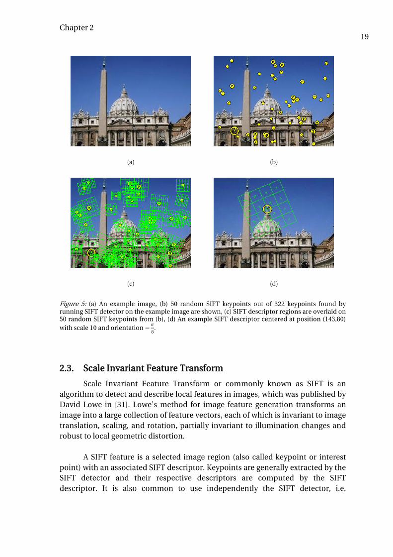
Scale Invariant Feature Transform or commonly known as SIFT is an algorithm to detect and describe local features in images, which was published by David Lowe in [31]. Lowe's method for image feature generation transforms an image into a large collection of feature vectors, each of which is invariant to image translation, scaling, and rotation, partially invariant to illumination changes and robust to local geometric distortion.

A SIFT feature is a selected image region (also called keypoint or interest point) with an associated SIFT descriptor. Keypoints are generally extracted by the SIFT detector and their respective descriptors are computed by the SIFT descriptor. It is also common to use independently the SIFT detector, i.e.

(a) (b)

(c) (d)

Figure 5: (a) An example image, (b) 50 random SIFT keypoints out of 322 keypoints found by running SIFT detector on the example image are shown, (c) SIFT descriptor regions are overlaid on 50 random SIFT keypoints from (b), (d) An example SIFT descriptor centered at position (143,80) with scale 10 and orientation −𝜋

8.

Chapter 2 20

computing the keypoints without descriptors, and the SIFT descriptor, i.e. computing descriptors of keypoints got from other detectors.

SIFT detector uses Difference of Gaussians (DoG) which is a grayscale image enhancement algorithm that contains subtraction of one blurred version of an original grayscale image from another, less blurred, version of the original. The blurred images are obtained by convolving the original grayscale image (single channel image with only intensity values) with Gaussian kernels having different standard deviations. Blurring an image using a Gaussian kernel suppresses only high-frequency spatial information and subtracting one image from the other preserves spatial information that lies between the ranges of frequencies that are preserved in the two blurred images. Thus, the difference of Gaussians is a band-pass filter that discards a certain range of spatial frequencies that are present in the original grayscale image.

The SIFT detector finds the keypoint locations as the maxima and minima of the result of the difference of Gaussians, applied in the scale space to a series of smoothed and resampled images. Low contrast candidate points and edge response points along an edge are discarded. These steps ensure that the keypoints are more stable for matching and recognition. After the keypoints are found using SIFT detector, dominant orientations are assigned to localized keypoints. A SIFT keypoint is generally represented as a circular image region with an orientation. It is described by a geometric frame of four parameters: the keypoint center coordinates x and y, its scale (the radius of the region), and its orientation (an angle expressed in radians).

A SIFT descriptor is a histogram of the image gradients that characterizes the appearance of a keypoint. SIFT descriptors, robust to local affine distortion (see chapter 4), are obtained by considering pixels around a radius of the keypoint location, blurring and resampling of local image orientation planes. Initially, a set of orientation histograms are created on 4x4 pixel neighborhoods with 8 bins each. These histograms are computed from magnitude and orientation values of samples in a 16 x 16 region around the keypoint such that each histogram contains samples from a 4 x 4 subregion of the original neighborhood region. The magnitudes values, around the 4 x 4 subregions of the keypoint, are further weighted by a Gaussian function with standard deviation equal to one half the width of the descriptor window. The descriptor then becomes a vector of all the values of these histograms. Since there are 4 x 4 = 16 histograms each with 8 bins the vector has 128 dimensions. This vector is then normalized to unit length in order to enhance invariance to changes in illumination. An example of feature extraction using SIFT is shown in Figure 5.

In the original SIFT proposed by Lowe, the Best-bin-first method [32] is used as a similarly measure which uses a modification of the k-d tree algorithm

Chapter 2 21

that can identify the nearest neighbors with high probability using only a limited amount of computation. The Best-bin-first algorithm uses a modified search ordering for the k-d tree algorithm so that bins in feature space are searched in the order of their closest distance from the query location.

SIFT has been used widely in many applications like object recognition, panorama stitching, and localization and mapping to name a few.

2.4. Histogram of Oriented Gradients

Histogram of Oriented Gradients (HOG) features were first proposed by Dalal and Triggs in [33]. Their basis lies in the assumption that local object appearance and shape within an image can be described rather accurately by the distribution of intensity gradients or edge directions, even without having precise knowledge of the corresponding intensity gradient or edge position.

The HOG feature descriptor is computed by dividing the image window into small spatial regions called cells and for each cell, accumulating the 1D histogram of gradient directions or edge orientations over the pixels of the cell. The combined histogram entries form the HOG feature descriptor. To improve invariance against illumination, shadow, etc., it is also useful to contrast-

(a) (b)

Figure 6: (a) An example image, (b) HOG descriptor of (a) showing the dominant orientations in the image.

Chapter 2 22

normalize by calculating a measure of the intensity across a larger region of the image, called a block, and then using this value to normalize all cells within the block. An example of HOG feature descriptor is shown in Figure 6.

HOG descriptors are generally sent into a classifier based on supervised learning [34]. One such system which is frequently used alongside HOG is the Support Vector Machine (SVM) classifier which is a binary classifier that uses an optimal hyper plane as a decision function. Once trained on images containing some particular object, the SVM classifier can make decisions regarding the presence of an object, such as a human being, in additional test images.

It can be seen that HOG is very similar to the SIFT descriptor. But the SIFT descriptor is applied only to the local keypoints or interest points, whereas the HOG is applied to the whole image.

HOG is widely used for applications like human detection, face detection and pedestrian detection.

2.5. GIST feature descriptor

The GIST feature descriptor was first proposed in [35] by Oliva and Torralba. GIST was developed with the idea to have a low dimensional representation of the scene called Spatial Envelope, which does not require any form of segmentation. The spatial envelope properties provide a holistic description of the scene where local object information is not taken into account. The idea behind the GIST descriptor is that specific information about object shape and identity is not a requirement for scene categorization and retrieval. The Spatial Envelope of an environmental scene may be described by a set of perceptual properties (naturalness, openness, roughness, expansion, and ruggedness) that represent the dominant spatial structure of a scene. These properties are related to the shape of the scene and are meaningful to human observers. These dimensions can be reliably estimated using spectral and coarsely localized information.

GIST divides the image into n x n windows and each window is represented by the texture it contains. This is accomplished by looking at the energy of a bank of oriented filters tuned at different orientation and scales. So if there are 8 filters tuned at 8 different orientations and 4 scales and the image is divided into 4x4 bins; we get a GIST descriptor of 512 dimensions. It is very similar to SIFT, but instead of applied to a local patch, it is applied to the entire image.

The similarity measure between two images using GIST descriptor is usually performed using Euclidian distance. An example of GIST descriptor is shown in Figure 7. GIST descriptor is used widely in scene classification and retrieval.

Chapter 2 23

2.6. Bag of Words (BoW)

The idea behind Bag of Words (BoW) model comes from natural language processing in which a text can be represented as an unordered collection of words, disregarding grammar and even word order. This idea has been exploited for images and Bag of Words (BoW), or more accurately bag of visual words, was first introduced by Sivic and Zisserman in [36] and for natural scenes later by Li Fei-Fei and Pietro Perona in [37].

An image can be described as a “bag of visual words” based on keypoints extracted as salient image patches. Keypoints contain rich local information of an image. They can be automatically detected using various detectors [38, 39] and represented by many descriptors. Keypoints are then classified into a large number of clusters so that those with similar descriptors are assigned into the same cluster. This is typically done using clustering algorithms like SVM or k-means. By treating each cluster as a “visual word” that represents the specific local pattern shared by the keypoints in that cluster, we have a visual word vocabulary describing all kinds of local image patterns. This visual word vocabulary is sometimes referred to as codebook. The visual word vocabulary size is important as if it is too small, visual words are not representative of all patches, and if the size is too large, quantization artifacts and over fitting tends to occur.

With its keypoints mapped into visual words, an image is represented as a vector containing the (weighted) count/histogram of each visual word in that image regardless of the position of the word. This representation is used as a feature descriptor for the image during retrieval.

(a) (b)

Figure 7: (a) An example image, (b) GIST representation of the example image.

Chapter 2 24

We can use the same similarity measures as in color histogram matching because the image is represented as a histogram of different visual words. Typically histogram intersection or Chi-square (𝜒2) histogram distance are used.

Bag of visual words is ideal for image classification and retrieval across different classes. However the disadvantage of BoW model is that it ignores the spatial relationships among the patches, which is very important in image representation. Researchers have thus proposed several methods to incorporate the spatial information [40-42] into the model.

2.7. Other methods

There are many other CBIR algorithms and methods for CBIR described in literature. The few relevant methods using principles differing from those explained in previous sections are given below:

2.7.1. Shape aware methods

Retrieval of images based on shape was proposed by Belongie et al. in [43]. This method measures the similarity between shapes and exploits it for image retrieval. A shape context descriptor is assigned to each point. A globally discriminative characterization is achieved by this shape context descriptor at a reference point that captures the distribution of remaining points relative to it. Corresponding points on two similar shapes will have similar shape contexts enabling to solve for correspondences as an optimal assignment problem. Given the correspondences, the transformation that best aligns the two shapes is estimated by using regularized thin-plate splines [44].

The similarity between the two shapes is computed as a sum of the matching errors between corresponding points, together with the term measuring the magnitude of the aligning transform. This method is best used while matching silhouettes, trademarks and handwritten digits.

2.7.2. Speeded Up Robust Features

Speeded Up Robust Features (SURF) descriptor was first proposed by Herbert Bay et al. in [45]. SURF is a fast and robust algorithm for local, similarity invariant representation and comparison. Inspired from the SIFT, to find the keypoints this algorithm uses an integer approximation of the determinant of the Hessian matrix applied to points in the image. To extract the vector of features, SURF uses the sum of the 2D Haar wavelet response around the keypoint, by making efficient use of integral images at several scales. Then SURF builds local features based on the histogram of gradient like local operators.

Chapter 2 25

The main interest of the SURF approach lies in its fast computation of operators in the box-space, enabling real-time applications such as tracking and object recognition.

2.7.3. Textons

Textons was proposed by Malik et al. in [46]. The term textons is analogous to a phoneme in speech recognition and represents the putative elementary units in texture perception. An image is passed through a bank of filters tuned to different orientations and scales and also with different elongations. At each pixel there is a vector of filter responses. By applying k-means to all the filter responses or to the vectors on a very large database, we can extract cluster centers. These cluster centers define the basic building blocks called textons.

Then, when a new image is presented, it is passed through the filter banks and its filter response is noted. Based on the filter response at every pixel, the center cluster which best describes the pixel is found and a histogram is built. This histogram is used as the feature descriptor of the image. Typically histogram intersection or Chi-square (𝜒2) histogram distance are used to perform the similarity calculation.

2.7.4. Machine learning methods

In recent years there has been increasing use of machine learning techniques in CBIR. Most of the methods using machine learning can be broadly classified into either online methods or offline methods. Online methods (IP connected) run the algorithms in the cloud. For example the LiRE project [47] as standard open source reference. The offline approaches have no IP connection available during the recognition stage. Discriminative learning algorithms are widely used [48, 49] in offline method for image recognition within a closed set of images. In the case of SVM-based image recognition and some deep-learning approaches such as the one used by Google image retrieval system [50], the main computationally intensive step is the machine learning training phase. This training step could be done on-line (cloud-based); however, the recognition step could be done off-line as it requires much less processing compared to the training phase.

3 Conclusions and summary of the chapter

Content Based Image Retrieval (CBIR) was introduced in this chapter along with the different scenarios and blocks that are used in a CBIR system. Also, the different features and similarity measures that are used in content based image retrieval were discussed.

Chapter 2 26

Reviews of several seminal CBIR algorithms and methods using different modalities that are currently used in the field were presented. The essential idea behind each algorithm/method was discussed together with the possible applications that best suit each algorithm/method.

Chapter 3

Image retrieval algorithms

In this chapter, two different image retrieval algorithms ‘Color Density Circular Crop’ (CDCC) and ‘DCT-Phase Match’ (DCTPM), developed as part of the PhD work, are presented. The CDCC and DCTPM algorithms are published at ISPA 2011 [3] and ICIP 2012 [4] respectively. This is followed by a low complexity image retrieval algorithm which combines the two algorithms to perform image retrieval in two stages. The chapter is organized as follows: In section 1 and section 2, ‘Color Density Circular Crop’ and ‘DCT-phase match’ algorithms are explained respectively. Both sections are followed by experimental evaluation of the algorithms. Finally in section 3, it is shown how the algorithms CDCC and DCTPM are combined to produce a two-stage low complexity image retrieval algorithm.

Chapter 3 28

1 Color Density Circular Crop

1.1. Introduction

“Colors are the smiles of nature” — Leigh Hunt

The color content of an image is a representative and convenient information, which is widely exploited in Content Based Image Retrieval (CBIR) systems. Initial work in CBIR using color was done by Swain and Ballard [20] who proposed image indexing based on color histograms. This was followed by two-decades of work by the research community [15] proposing a variety of CBIR algorithms based on color histograms and, more recently, on different forms of region-based color characterization.

Color histograms provide useful information for CBIR, are invariant to translation and rotation, and vary very gradually to change in scale and occlusion. A color histogram is a representation of the combined distribution of colors in an image, obtained by counting the number of pixels of each of given sets of color ranges in two-dimensional (2D) or three-dimensional (3D) color spaces. 2D color spaces with no intensity information, such as rg-chromaticity or hue-saturation, are typically used. If the number of bins per dimension is Q, the length of the feature vector is 𝑄2. For good retrieval accuracy, the color space needs to be finely represented, with a large enough Q. This yields to large feature vector lengths, in the order of a few hundreds to one hundred, the latter with drastic quantization of the color space and subsequent reduction in retrieval accuracy. Large feature vectors are impractical both in terms of storage space requirements and computational complexity.

In this subsection, an introduction to the color fundamentals and color spaces is presented. These concepts form the groundwork to better understand the ‘Color Density Circular Crop’ algorithm[3] which follows in the next subsection.

1.1.1. Color fundamentals

In 1666, Sir Isaac Newton discovered that when a beam of sunlight passes through a glass prism, the emerging beam of light is not white but consists of a continuous spectrum of colors ranging from violet at one end to red at the other [51]. Newton divided the spectrum into seven colors: red, orange, yellow, green, blue, indigo, and violet. Newton chose seven colors out of a belief, derived from the ancient Greek sophists, that there was a connection between the colors, the musical notes, the days of the week, and the known objects in the solar system. It was until the early 19th century with seminal works by Sir William Herschel, Johann Wilhelm Ritter, Thomas Young, Hermann von Helmholtz, and others [52], that the concept of visible spectrum became more definitive and visible light, as

Chapter 3 29

we known today, was thought to be composed of a relatively narrow band of frequencies in the electromagnetic spectrum spanning from approximately 400 to 700 nm.

The colors human and some animals perceive in an object are determined by the nature of the light reflected from the object [53]. A body that reflects light that is balanced in all visible wavelengths appears white to the observer. However, a body that favors reflectance in a limited range of the visible spectrum exhibits some shades of color. For example, red objects reflect light with wavelengths primarily in the 630 to 700 nm range while absorbing most of the energy at other wavelengths.

According to the trichromatic theory proposed by Thomas Young and Hermann von Helmholtz [54], the sensation of color is produced by selectively exciting three classes of receptors in the eye. Certain frequencies in the visible light spectrum will excite certain receptors producing the effect of color. Furthermore, if we provide the same stimulus to these receptors from two different sources, the two sources will appear to have the same color.

In color imaging there are two basic ways of producing this selective excitation: additive color and subtractive color. Additive color is used with active light emitting systems in which the light from different sources is added to produce the perceived color. Subtractive color is used in passive systems, in which light from given sources is selectively absorbed at different wavelengths, leaving only the wavelengths that will be perceived as the desired colors. Colors produced by other physical processes, such as reflection and interferences, can be seen as alternative ways of creating the additive and subtractive color.

1.1.2. Color spaces

Color space [21] is a mathematical model that facilitates the representation of colors in some standard, generally accepted way. Many representations of color images are possible. The trichromatic theory tells us that, ideally, three components should be sufficient to represent a color image. However, output devices are limited, so not all colors can be obtained.

RGB color model

RGB color model is an additive color model in which the red, green, and blue color intensities are added together in various ways to reproduce a broad array of colors. This model is based on the Cartesian coordinate system. The color subspace is the cube shown in Figure 8(a), in which RGB values are at three corners; cyan, magenta, and yellow are at the three other corners; black is at the origin and white is at the corner farthest from the origin. In this model, the grayscale, i.e., points with equal RGB values extends from black to white along the line joining these two points.

Chapter 3 30

Consider an RGB image in which each of the red, green, and blue images is an 8-bit image. Under these conditions each RGB color pixel is said to have a depth of 24 bits. The term full-color image is often used to denote a 24-bit RGB color image. The total number of possible colors in a 24-bit RGB image is (28)3 = 16,777,216.

YUV color model

The YUV color model imitates human vision. Humans are able to discern the contents of a color RGB image presented in the two main forms, as an original RGB color image or as a grayscale image (image with only intensity information). The YUV color format describes color by using the color components: luminance and chrominance. The luminance component (Y) represents the brightness information of a color; the chrominance components (U and V) contain the color differences. The YUV color format was developed for analog TV transmission to provide compatibility between black-and-white television and color television. The black-and-white systems used only luma (Y) information; color information

1 http://www.flickr.com/photos/bhaskardutta/6701663729/ - with due permission from the photographer

(a) (b) (c)1

(d) (e) (f)

Figure 8: (a) RGB 24-bit color cube, (b) YCbCr color model visualization, (c) Full-color image, (d)-(f) Red, Green, and Blue channels of the full-color image in (a).

Chapter 3 31

(U and V) was added in such a way that a black-and-white receiver would still display a normal black-and-white picture. Color receivers decode the additional color information to display a color picture.

YCbCr color model

The YCbCr color format is a scaled and offset version of the YUV color format. It also consists of a luminance component (Y) and two chrominance components (Cb and Cr). The term YCbCr is often confused with YUV, which is used for analog composite color video standards like PAL, NTSC or SECAM. In contrast to YUV, YCbCr is used in the context of digital image and video processing, especially, for JPEG images and MPEG video encoding. There are several YCbCr sampling formats that are widely used, such as 4:4:4, 4:2:2, 4:1:1, and 4:2:0. Among these the 4:2:2 is the most popular sampling format in cameras where the two chroma components are sampled at half the sample rate of luma component and is typically interleaved and represented as UYVY format.

Both color formats, YCbCr and YUV, describe color by using luminance and chrominance. However, the coefficients for color conversion from and to RGB color format are different. The conversion from RGB space to YCbCr space is given by:

𝑌 = 77𝑅 + 150𝐺 + 29𝐵

256

𝐶𝑏 = 𝐵 − 𝑌

𝐶𝑟 = 𝑅 − 𝑌

(12)

The conversion from YCbCr space to RGB is given by:

𝑅 = 𝑌 + 𝐶𝑟

𝐺 = 𝑌 − 0.193𝐶𝑏 − 0.513𝐶𝑟

𝐵 = 𝑌 + 𝐶𝑏

(13)

1.2. CDCC algorithm

An efficient image retrieval algorithm, developed as part of the PhD work, in which the image color characteristics are modeled using small-sized feature vectors, yielding to fast retrieval and low storage requirements is explained in this subsection. The extracted image features are the color densities of concentric circular zones encompassing the detected edge-pixels. The proposed algorithm is invariant to Rotation, Scaling, and Translation (RST). As the computational load is low, the proposed algorithm is suited for implementation as the image retrieval algorithm for pre-selection stage in portable handheld devices.

Chapter 3 32

The proposed algorithm is divided into Feature extraction, and Similarity calculation and Image retrieval, as explained in subsections 1.2.1 and 1.2.2 respectively.

1.2.1. Feature extraction

As seen in chapter 2, features are distinctive attributes that denote a piece of information which is relevant for solving a computational task such as image retrieval and feature extraction is the procedure to obtain features in terms of local neighborhood operations applied to an image.

In our algorithm, the feature extraction process consists of circular segmentation, concentric cropping, calculation of the color density, and normalization as explained in the subsections below. The resulting features are called the ‘Color Density Circular Crop’ features or CDCC features.

Circular segmentation

Circular segmentation involves separating the image into a circle which encompasses the important and relevant information of the image. To perform this circular segmentation, we use the Canny edge detector [55] on the query image I, to obtain the Edge-Set (E) containing the K edge-pixels representing all the edges in the image, as follows:

𝐸 ≡ �𝑃𝑖

𝐾

𝑖=1

, (14)

where 𝑃𝑖 is the ith pixel for which an edge was found, represented by its coordinates {𝑥𝑖, 𝑦𝑖}.

We encompass all the edge-pixels with a circle of center {𝑥𝑐,𝑦𝑐} and radius 𝑟𝑐. In order to compute the center we first calculate the extrema points of the Edge-Set as follows:

𝑥𝑀𝑎𝑥 = 𝑠𝑢𝑝{𝑥𝑖|𝑃𝑖 ∈ 𝐸},

𝑥𝑀𝑖𝑛 = 𝑖𝑛 𝑓{𝑥𝑖|𝑃𝑖 ∈ 𝐸},

𝑦𝑀𝑎𝑥 = 𝑠𝑢 𝑝{𝑦𝑖|𝑃𝑖 ∈ 𝐸},

𝑦𝑀𝑖𝑛 = 𝑖𝑛 𝑓{𝑦𝑖|𝑃𝑖 ∈ 𝐸},

(15)

Then we calculate the center using these extrema points:

{𝑥𝑐, 𝑦𝑐} = �𝑥𝑀𝑎𝑥 + 𝑥𝑀𝑖𝑛

2,𝑦𝑀𝑎𝑥 + 𝑦𝑀𝑖𝑛

2� , (16)

Chapter 3 33

We calculate the radius as the minimum distance from the center which is required to circumscribe all the 𝐾 edge-pixels 𝑃𝑖 in the Edge-Set (𝐸):

𝑟𝑐 = 𝑠𝑢𝑝 � � ��( (𝑥𝑖 − 𝑥𝑐)2 + (𝑦𝑖 − 𝑦𝑐)2)�{𝑖|𝑃𝑖∈𝐸}

� , (17)

Concentric Circular Crop

The segmented circular region, with the center {𝑥𝑐, 𝑦𝑐} and the radius 𝑟𝑐, is cropped into 𝑞 concentric zones, 𝑍ℎ, using 𝑞 concentric circles described by:

(𝑥 − 𝑥𝑐)2 + (𝑦 − 𝑦𝑐)2 = �ℎ 𝑟𝑐𝑞�2

, (18)

where ℎ = 𝑞, 𝑞 − 1, . . ., 1. In Figure 9 we show an example of circular segmentation and concentric cropping of an image when 𝑞 = 4. The four concentric circular zones 𝑍1 to 𝑍4 are shown at the right of the image.

Color Density calculation

Color density describes the amount of a specific color stored in a given section of an image. In particular, it tells us the amount of red, green, and blue colors present in a given section of an image.

The color density of the red, green, and blue channels of each of the 𝑞 concentric zones is calculated, by adding the contribution of each of the pixels inside the zone:

𝑅ℎ = � 𝑟𝑖{𝑖|𝑃𝑖 ∈ 𝑍ℎ}

; 𝐺ℎ = � 𝑔𝑖;{𝑖|𝑃𝑖 ∈ 𝑍ℎ}

𝐵ℎ = � 𝑏𝑖 ,{𝑖|𝑃𝑖 ∈ 𝑍ℎ}

(19)

where 𝑅ℎ, 𝐺ℎand 𝐵ℎ are the color densities of the red, green, and blue channels for the concentric zone 𝑍ℎ, and 𝑟𝑖, 𝑔𝑖, and 𝑏𝑖 are the RGB color intensities of the pixel 𝑃𝑖.

Color Density normalization

Finally the calculated color densities are normalized by 𝑟𝑐2 and assembled together in a feature vector of length 𝐿 = 3𝑞:

Chapter 3 34

𝒇 = �� 𝑅ℎ𝑟𝑐2

; 𝐺ℎ𝑟𝑐2

; 𝐵ℎ𝑟𝑐2�

𝑞

ℎ=1

. (20)

The vector 𝒇 constitutes the CDCC (“Color Density Circular Crop”) extracted features.

These features are RST invariant: Rotation invariance is due to the use of circular zones, scale invariance is achieved with normalization of the color densities by 𝑟𝑐2, whereas translation invariance is due to the calculation of the center using the edge-pixel locations.

For a typical value of 𝑞 = 4 we have a feature vector of length 𝐿 = 12. As the feature vector length is very small, so are the retrieval time and the memory used for storing the pre-calculated feature vectors. Besides, the complexity of the feature calculation is low, compared with existing methods.

1.2.2. Similarity calculation and image retrieval

For every image stored in the database, the feature vector 𝒇 = {𝑓1,𝑓2, … ,𝑓𝐿} is pre-calculated and stored. When a query image is presented, the feature vector of the query is calculated and compared with the feature vector of each of the images stored in the database, using the 𝐿1 distance:

𝑑�𝐼𝑛, 𝐼𝑞𝑢𝑒𝑟𝑦� = ∑ �[𝑓𝑖]𝐼𝑛 − [𝑓𝑖]𝐼𝑞𝑢𝑒𝑟𝑦�𝐿𝑖=1 , (21)

where 𝐼𝑛 is the n-th image of the database of size N. The N distances are calculated and ordered, and the M smallest distances are selected:

𝑑�𝐼𝑛1, 𝐼𝑞𝑢𝑒𝑟𝑦� ≤ 𝑑�𝐼𝑛2, 𝐼𝑞𝑢𝑒𝑟𝑦� ≤ ⋯ ≤ 𝑑�𝐼𝑛𝑀, 𝐼𝑞𝑢𝑒𝑟𝑦�. (22)

Figure 9: An example of circular segmentation and concentric cropping of an image into 4 concentric regions.

Chapter 3 35

The M retrieved images are the M images {𝐼𝑛1, 𝐼𝑛2, … , 𝐼𝑛𝑀} corresponding to the M smallest distances between the features of the query image and the features of the images in the database.

1.3. Experimental evaluation

In the next subsections we present the databases used for experimental evaluation, testing procedure, and results.

1.3.1. Experimental databases

Two databases, one for pictograms and one for pictures were used during the tests. The pictogram database contains 4859 pictograms from the Picture Communication Symbols (PCS) set [56]. The pictograms were stored in JPEG format with 85% quality, and VGA resolution (640 × 480). The picture database contains the 1000 pictures of the COREL photograph data set used in [57] which are JPEG compressed color images with QVGA (320 × 240) resolution. We refer to these two databases as the “clean pictogram database” and the “clean picture database”.

Additionally, a set of 50 representative pictograms and 50 representative pictures were chosen manually from the clean databases. These images were printed and acquired using a fixed focus OV7675 VGA camera from Omnivision [58]. These two sets of 50 images constitute what we call the “real condition pictogram database” and the “real condition picture database”.

1.3.2. Testing procedure

The proposed retrieval algorithm was implemented in MATLAB. For testing, we have used the two clean databases presented in subsection 1.3.1, and 𝑞 = 4, which gives a feature vector length of 𝐿 = 12. Every image within the database is successively used as query, running the search for this image on the entire database. With each query image, we run eight searches, each with different conditions: no RST, rotation by an angle 𝜃 of 30, 60 and 90 degrees, scaling by a factor 𝑠 of 0.5, 0.75 and 1.25, and translation by (∆𝑥,∆𝑦) = (100,100). After running each search we recorded the 30 best matches. We then calculated the image retrieval precision 𝑝 as:

𝑝 = ∑ 𝑉𝑘𝑁𝑘=1

𝑁 , (23)

where 𝑉𝑘 = 1 when the query is contained in the 𝑀 retrieved images, and 𝑉𝑘= 0 otherwise. 𝑁 is the total number of images in the database on which the search is run. We have computed the precision for 𝑀 = 1, 10 and 30, i.e. for the case of retrieval of the top 1, top 10 and top 30 best matches.

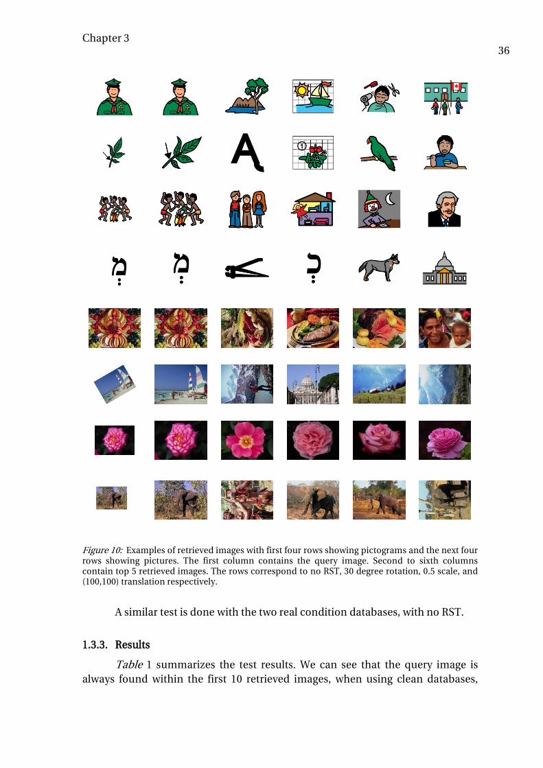
Chapter 3 36

A similar test is done with the two real condition databases, with no RST.

1.3.3. Results

Table 1 summarizes the test results. We can see that the query image is always found within the first 10 retrieved images, when using clean databases,

Figure 10: Examples of retrieved images with first four rows showing pictograms and the next four rows showing pictures. The first column contains the query image. Second to sixth columns contain top 5 retrieved images. The rows correspond to no RST, 30 degree rotation, 0.5 scale, and (100,100) translation respectively.

Chapter 3 37

and within the first 30 retrieved images, when using real condition databases. Figure 10 illustrates an example of the first 5 retrieved images, for a pictogram with no RST, a pictogram with 30 degrees rotation, a pictogram scaled by 0.5 and a pictogram translated by (100,100). It also shows an example of a picture with no RST, with 30 degrees rotation, scaled by 0.5 and translated by (100,100).

The tests were performed on MATLAB running on an Intel Core 2 Duo processor with 2.4 GHz. When the feature vector length is 𝐿 = 12, the average time to retrieve 𝑀 = 30 images from the 𝑁 = 4859 pictogram database is 303.5ms. This retrieval time is divided into the time to extract the CDCC features of the query, and the time to find the best 𝑀 matches from the database. The computational complexity of the CDCC feature extraction also affects the time needed for pre-calculating and storing the features for each database image. The computational time for extracting the CDCC features vary based on the image content (amount and location of the edge-pixels). The average time for extracting the CDCC features of the 4859 pictograms database is 291.5 ms. The time needed to find the M best matches is the addition of the distance calculation time and the sorting time. Distance calculation time is proportional to the feature vector length 𝐿 = 12, and to the database size 𝑁 = 4859. The average time taken for Distance calculation is 2.168 ms.

Pictograms Pictures

M=1 M=10

M=30

M=1 M=10 M=30

Cle

an d

atab

ases

No RST 1 1 1 1 1 1

Rotation

θ = 30° 0.849 1 1 0.832 1 1

θ = 60° 0.867 1 1 0.828 1 1

θ = 90° 1 1 1 1 1 1

Scale

s = 0.5 0.979 1 1 0.729 1 1

s = 0.75 0.978 1 1 0.849 1 1

s = 1.25 0.991 1 1 0.965 1 1

Translation (∆x,∆y) = (100,100) 1 1 1 0.987 1 1

Real condition databases 0.62 0.92 1 0.68 0.86 1

Table 1: Summary of the results for the different tests performed using CDCC.

Chapter 3 38

2 DCT-phase match

2.1. Introduction

Nowadays, images are usually stored and transmitted in compressed form. Image transform is an integral component of compressed images. By processing images directly in the transformed (compressed) domain, important savings in terms of computation, memory requirements, and processing speed can be made. Multiple compressed-domain image retrieval algorithms are proposed in the literature [59].

Discrete Cosine Transform (DCT) [60] is an essential processing block of JPEG compression. Many algorithms have been proposed in literature [61-65] which use DCT-phase data to match and retrieve images from databases. These algorithms generally work well with clean images. However, a key challenge is to keep their good performance in case of distortions or occlusions.

In the next subsections, an introduction to the Discrete Cosine Transform is presented giving the foundations to better understand the ‘DCT-phase match’ algorithm [4] developed during the PhD work.

2.1.1. Discrete Cosine Transform

The human visual response is dependent on the spatial frequency. If we could decompose the image into a set of waveforms, each with a particular spatial frequency, we might be able to separate the image structure that the eye can see from the structure that is imperceptible. The Discrete Cosine Transform can provide a good approximation to this decomposition [66].

The DCT is a linear transform similar to the Discrete Fourier Transform (DFT). The DCT operates on function samples of finite length and to be able of performing DCT expansion, a periodic extension of this function samples is required. This extension must be an even function.

Let 𝑠(𝑛,𝑚) be a pixel intensity at location (𝑛,𝑚) of an W × H image. The DCT of 𝑠(𝑛,𝑚) is denoted by 𝑆𝐷𝐶𝑇(𝑗,𝑘). Then the forward DCT-II [67] can be represented as a 2-dimmensional 8 × 8 sequence given by:

𝑆𝐷𝐶𝑇(𝑗,𝑘) =𝐶(𝑗)

2𝐶(𝑘)

2 � � 𝑠(𝑛,𝑚)cos �

(2𝑚 + 1)𝑘𝜋16

� cos �(2𝑛 + 1)𝑗𝜋

16�

7

𝑚=0

7

𝑛=0

. (24)

It should be noted that in Eq.(24), we deal with the case where W × H is equal to 8 × 8, as we normally use sub-blocks of this size to compute the DCT for images.

The inverse discrete cosine transform is given as:

Chapter 3 39

𝑠(𝑛,𝑚) = �𝐶(𝑗)

2

7

𝑗=0

�𝐶(𝑘)

2

7

𝑘=0

𝑆𝐷𝐶𝑇(𝑗,𝑘) cos �(2𝑚 + 1)𝑘𝜋

16� cos �

(2𝑛 + 1)𝑗𝜋16

�, (25)

where

𝐶(𝑗) = �1√2

, 𝑗 = 0

1, 𝑗 > 0 ,

𝑠(𝑛,𝑚) = pixel intensity at location (𝑛,𝑚),

𝐶(𝑘) = �1√2

, 𝑘 = 0

1, 𝑘 > 0 ,

𝑆𝐷𝐶𝑇(𝑗,𝑘) = 2-D DCT coefficient.

Figure 11: Illustration showing 64 basis functions for a 8 x 8 matrix.

Chapter 3 40

These cosine functions are called the basis functions of the DCT. The DCT coefficients 𝑆𝐷𝐶𝑇(𝑗,𝑘), then can be regarded as the weights to each basis function. For 8x8 matrices, the 64 basis functions are illustrated by Figure 11.

The main advantage of DCT is that it provides energy compaction. The low frequency coefficients have typically larger magnitude and the high frequency coefficients have typically smaller magnitude. Thus, most of the information in the image is compacted into the lower frequency coefficients i.e., the coefficients at the ‘upper-left’. This energy compaction is leveraged for compression in JPEG and MPEG. Figure 12 shows the percentage of cumulative energy versus the number of coefficients for both DCT and DFT using a Gaussian input with standard deviation of 0.4. We can see from the plot that the DCT compacts most of the energy with fewer coefficients than the DFT.

2.1.2. JPEG compression

JPEG is a standardized image compression mechanism. The acronym JPEG stands for the Joint Photographic Experts Group, the name of the committee that created the JPEG standard and also other still picture coding standards. The JPEG standard specifies a family of image codecs, which defines how an image is compressed into a stream of bytes and decompressed back into an image. The four JPEG modes of operation are the sequential DCT-based mode, the progressive DCT-based mode, the sequential lossless mode, and the hierarchical mode [66].

The most common mode of operation is the sequential DCT-based mode and a particular restricted form of this sequential DCT-based mode of operation is called the “baseline” JPEG. The “baseline” JPEG specifies the minimal subset of the standard that a JPEG-aware application should support. DCT-based and more generally transformed based encoding algorithms are always lossy by nature. DCT algorithms are capable of achieving a high degree of compression with only minimal loss of data. But, this scheme is effective for compressing images in which the differences between adjacent pixels are small. The baseline standard specifies eight bits per input sample. The baseline JPEG compression can be divided into five steps:

1. Transform the color space of the image from RGB to YCbCr using Eq. (12), where luminance component (Y) is related to the brightness and chrominance components (Cb and Cr) are related to the color of the image.

2. Down-sample chrominance components by averaging groups of pixels together, usually by a factor of 2. This exploits the fact that the human eye is less sensitive to fine color details than to fine brightness details.

3. The image is split into blocks of 8×8 pixels, and for each block, each of the Y, Cb, and Cr data undergoes the Discrete Cosine Transform (DCT) using Eq. (24).

Chapter 3 41

4. The obtained DCT coefficients are quantized using weighting functions optimized for the human eye. Human vision is much more sensitive to small variations in color intensity or brightness over large areas than to high-frequency brightness variations. Therefore, the magnitudes of the high-frequency components are stored with a lower accuracy than the low-frequency components. The quality setting of the encoder (for example 50 or 75 on a scale of 0–100 in the Independent JPEG Group's library) affects to what extent the resolution of each frequency component is reduced.

5. The resulting quantized DCT coefficients for all the 8 × 8 blocks are further compressed by using entropy encoder followed by a Huffman variable word-length algorithm.

The decoding process reverses these steps, except the quantization because it is irreversible. In the rest of the document, when we refer to JPEG, we actually refer to this “baseline” JPEG compression.

Figure 12: Illustration of energy compactness of DCT versus DFT on a centered Gaussian input with standard deviation of 0.4.

Chapter 3 42

2.2. DCTPM algorithm

We have developed a DCT-phase only image retrieval algorithm for occluded and fused images [68] first published in [4]. This algorithm utilizes a novel correlation metric for ternary-valued DCT-phase. A new region merging method is also proposed, which is used to reconstruct the non-occluded regions of the image.

2.2.1. DCT-phase for image retrieval

A study on the significance of DCT-phase in images was reported in [62], where it is shown that the DCT-phase, in spite of its binary value {0,𝜋} (that corresponds to either positive or negative DCT-coefficient), conveys significant amount of information about its associated image. In this subsection we explain the DCT-phase of an image and its ternary-valued representation used for the new correlation metric proposed in subsection 2.2.2.

DCT-phase of an image

Let 𝑠(𝑛,𝑚) be a 2-dimmensional W × H sequence. The DCT of 𝑠(𝑛,𝑚) is denoted by 𝑆𝐷𝐶𝑇(𝑗,𝑘). It can be expressed in terms of its absolute value, |𝑆𝐷𝐶𝑇(𝑗,𝑘)|, and its corresponding phase term, 𝑆𝐷𝐶𝑇′ (𝑗,𝑘) as:

𝑆𝐷𝐶𝑇(𝑗,𝑘) = |𝑆𝐷𝐶𝑇(𝑗,𝑘)| 𝑆𝐷𝐶𝑇′ (𝑗,𝑘). (26)

as 𝑆𝐷𝐶𝑇(𝑗,𝑘) is real valued, 𝑆𝐷𝐶𝑇′ (𝑗,𝑘) can take two values, i.e. 𝑆𝐷𝐶𝑇′ (𝑗,𝑘) ∈{+1,−1} corresponding to {0,𝜋}. Hereafter we refer to 𝑆𝐷𝐶𝑇′ (𝑗,𝑘) as the DCT-phase term.

(a) Original (b) DCT Magnitude only (c) DCT Phase only

Figure 13: (a) Monochrome test image, (b) IDCT applied to the magnitude array with constant phase, (c) Reconstruction when IDCT is applied over binary-valued phase arrays, when magnitude is set to one.

Chapter 3 43

The “DCT-phase only image” is the inverse DCT [69] of 𝑆𝐷𝐶𝑇′ (𝑗,𝑘) whereas the “DCT-magnitude only image” is the inverse DCT of |𝑆𝐷𝐶𝑇(𝑗, 𝑘)|. Figure 13 shows an example of an image, its DCT-magnitude only image and its DCT-phase only image. As we can see from the example, high amount of information is conveyed in the DCT-phase.

Most digital images are compressed with JPEG compression standard, which uses DCT on the 8 × 8 blocks of the image. In the JPEG compressed images, the DCT coefficient signs of the 8 × 8 blocks can be obtained directly, with low complexity computation, by partial entropy decoding of the encoded bitstream [62]. We thus decided to perform image retrieval in the compressed domain using the DCT-phase of the 8 × 8 blocks of the image as explained in the following subsections.

DCT-phase representation

We represent the DCT-phase with values from the ternary set {+1, 𝛼,−1}, where the ‘+1’ symbol corresponds to 𝑆𝐷𝐶𝑇′ (𝑗,𝑘) = +1 (0 phase), and the ‘−1’

Figure 14: Block diagram of the proposed DCT phase based image retrieval algorithm for occluded images.

Chapter 3 44

symbol corresponds to 𝑆𝐷𝐶𝑇′ (𝑗,𝑘) = −1 (‘π’ phase). The symbol ‘𝛼’ corresponds to zero magnitude of the DCT coefficients, |𝑆𝐷𝐶𝑇(𝑗,𝑘)| = 0.

This ternary-valued representation provides an improvement over the binary-valued representation {+1,−1}, as it removes the ambiguity of phase for zero magnitude DCT coefficients, which occur quite frequently after the quantization step, while compressing images in JPEG format.

2.2.2. Retrieval algorithm for occluded images

Figure 14 shows the block diagram of the proposed DCT phase based image retrieval algorithm for occluded images. This algorithm first finds the best matching image, using the proposed correlation metric with ternary-valued DCT-phase which improves matching performance, especially in the case of occluded images as shown in section 2.3. After the best matching image is found, intermediate values of the correlation metric calculation are used for region merging in order to retrieve the non-occluded portion of the image.

Correlation metric

As explained in section 2.2.1, we first compute the ternary-valued DCT-phase of the 8 × 8 blocks of the query image 𝐼𝑄 with horizontal and vertical pixel resolution of W and H respectively, obtaining a W × H matrix of ternary symbols. Hence forth, we express this matrix as 𝜃𝑄𝑢𝑒𝑟𝑦ℎ𝑘 , where h = 0,1,…,(H/8)-1 and k =

0,1,…,(W/8)-1. The indexes h and k identify the corresponding 8 × 8 block of the image 𝐼𝑄.

To correlate a query image 𝐼𝑄 and a reference image 𝐼𝑅𝑒𝑓, we first multiply

element-by-element their corresponding DCT-phase arrays, θQueryhk and θReferencehk :

𝜃𝑄,𝑅𝑒𝑓ℎ𝑘 (𝑖, 𝑗) = 𝜃𝑄𝑢𝑒𝑟𝑦ℎ𝑘 (𝑖, 𝑗) ∙ 𝜃𝑅𝑒𝑓𝑒𝑟𝑒𝑛𝑐𝑒ℎ𝑘 (𝑖, 𝑗). (27)

Table 2 shows the possible outcomes for such a multiplication where

θQueryhk (i, j) and θReferencehk (i, j) can take values {+1, 𝛼, −1} and the outcome belongs

to the quinary set {+1, 𝛼,α2,−𝛼,−1}. An exact match is found when the outcome belongs to {+1, α2}, which forms the principal diagonal of the matrix of possible outcomes given in Table 2.

Chapter 3 45

After performing the multiplication between the query and the reference image, each element of the resultant arrays is assigned one of three possible “labels”, Valid (V), Not-valid (N) and a Don’t care (X), corresponding to {+1}, { 𝛼,−𝛼,−1} and {α2} respectively, as shown in Table 3.

The rationale behind labeling {𝛼2} as don’t care (X) is that in JPEG compression the majority of DCT coefficient values are quantized to zero and these zero-valued DCT coefficients do not provide significant information for image retrieval using phase correlation.

The similarity between the query and the reference image is calculated using the following correlation metric:

𝑑�𝐼𝑄 , 𝐼𝑅𝑒𝑓� =∑(𝑉)

∑(𝑉) + ∑(𝑁) . (28)

Using Eq.(28), we calculate the correlation between the query image and each image within the searched database. The best matching image in the searched database corresponds to the maximum correlation value.

For clean non-occluded images, i.e. no distortion between the query image and its reference stored in the database, the similarity measure for the best match is equal to one. If there is occlusion (but no other distortion), the similarity measure gives the percentage of the non-occlude area.

Region merging

In the case of occluded images, once the best match is retrieved from the database using the metric of Eq.(28), we can find the region in the image which is not occluded by performing region merging using the labels (Valid, Not-valid, Don’t Care) assigned previously in the DCT-phase domain.

θReferencehk (i, j)

+1 𝛼 −1

θQueryhk (i, j)

+1 +𝟏 𝛼 −1

𝛼 𝛼 𝛂𝟐 −𝛼

−1 −1 −𝛼 +𝟏

Table 2: Possible outcomes for 𝜃𝑄,𝑅𝑒𝑓ℎ𝑘 (𝑖, 𝑗) from Eq. (27).

Chapter 3 46

For the array θQ,Refhk of a given 8 × 8 block to which labels (V,N,X) have been

assigned , we compute the mean of the number of labels which are either valid or don’t cares. That is:

𝑚ℎ𝑘 = 1

64�� 1{𝑉,𝑋}�θQueryhk (i, j)�

7

𝑗=0

.7

𝑖=0

(29)

If this mean is above a given threshold, 𝑚𝑡ℎ𝑟𝑒𝑠 , the 8 × 8 block is classified as a matching block. After all the matching blocks are found, those which are connected to at least one adjacent matching block are retained, and the other are discarded. The non-occluded portion of the retrieved image is then formed by all the retained blocks.


In the next subsubsections we present the databases used for the experimental evaluation, the testing procedure and the obtained results.

2.3.1. Experimental database

The reference database used for the tests contains 1000 images from the COREL photograph data set used in [57] which are natural color JPEG compressed images with QVGA resolution (320×240).

The reference database was randomly divided into two datasets known as ‘datasetA’ and ‘datasetB’ each containing 500 images. A sample image from ‘datasetA’ is shown in Figure 15(a).

An “occluded image database”, called ‘datasetOcclude’, was generated by occluding 37.5% of each image in ‘datasetA’ with part of an image in the ‘datasetB’: the lower-left triangular portion of the image was replaced by the same

θReferencehk (i, j)

+1 𝛼 −1

θQueryhk (i, j)

+1 𝐕 N N

𝛼 N 𝐗 N

−1 N N 𝐕

V = Valid

N = Not-valid

X = Don’t care

Table 3: Labels assigned to possible outcomes.

Chapter 3 47

region from the occluding image. A sample image from this dataset is shown in Figure 15(b).

To generate a database of fused images, called ‘datasetFused’, each image in the ‘datasetA’ was merged with an image from ‘datasetB’ using wavelet decomposition by taking the mean for both approximations and details coefficients (wfusimg function in MATLAB). A sample image from this dataset is shown in Figure 15(c).

Images in ‘datasetA’ were JPEG compressed with two different compression ratios (CR): 60% and 30%; creating two compressed databases ‘dataset30CR’ and ‘dataset60CR’. A sample image from dataset30CR is shown in Figure 15(d).

2.3.2. Testing procedure and results

The proposed DCT phase based image retrieval algorithm was implemented in MATLAB. The algorithm was tested under the different conditions of occlusion, fusion and compression, corresponding to the datasets explained in subsection 2.3.1. When testing a dataset, each image in a dataset was successively used as the query, searching it on the reference database. The best match always corresponded to the query image.

The ratio of the correlation of the Best Match (BM) to the correlation of the Second Best Match (SBM) is used to measure the performance and robustness of the retrieval algorithm. When testing a dataset, we calculate the mean and the standard deviation of this ratio. A high mean with a low standard deviation is an indication of good performance and robustness.

Figure 15(e) to Figure 15(h) show the histograms of the BM/SBM correlation ratio for each dataset using the proposed algorithm. Column 1 of Table 4 gives the summary of the resulting mean (m) and standard deviation (σ) of the BM/SBM correlation ratio, for the different datasets tested with our proposed algorithm.

It can be seen that the proposed DCT phase based image retrieval algorithm provides a good distance between BM and SBM not only for the occluded set but also for reference, fused, and JPEG compressed images.

The proposed DCT phase based algorithm was compared with other state of the art DCT-phase based algorithms for image retrieval [62], [61]. The algorithm proposed in [61] uses a binary value for phase i.e., {+1,−1} whereas [62] uses ternary-valued {+1, 0,−1} phase, but with a correlation metric that does not treat differently the “α2” case, i.e. the case in which both DCT-magnitudes are zero (see Subsection 2.2.1).

Chapter 3 48

Our region merging algorithm successfully retrieved the non-occluded regions of the images. Figure 16 shows an example of our proposed region merging algorithm (b) and of region merging using the DCT-phase representation of [61] and [62] in (c) and (d) respectively. A threshold (mthres) of 0.75 was used. It is seen that the DCT-phase representation of [61] and [62] is not suitable for accurately retrieving the non-occluded portion of the image.

From Table 4 it can be seen, by comparing the mean of the BM/SBM correlation ratios, that the proposed image retrieval algorithm outperformed other algorithms [62], [61] by an average factor of 2.46 and 2.32 respectively over different datasets. We can see that the algorithm proposed in [62] which also used a ternary-valued DCT-phase representation, showed a lower mean than [61] which used a binary-valued DCT-phase. However, algorithm [62] had the least standard deviation.

Proposed algorithm

Algorithm in [62]

Algorithm in [61]

Dataset m σ M σ m σ

Reference database

3.97 0.36 1.26 0.09 1.14 0.18

datasetOcclude 2.52 0.26 1.16 0.06 1.19 0.09

datasetFused 2.21 0.49 1.19 0.08 1.31 0.14

dataset30CR 2.37 0.32 1.13 0.05 1.04 0.03

dataset60CR 3.73 0.39 1.26 0.09 1.39 0.18

Table 4: Summary of test results for different datasets.

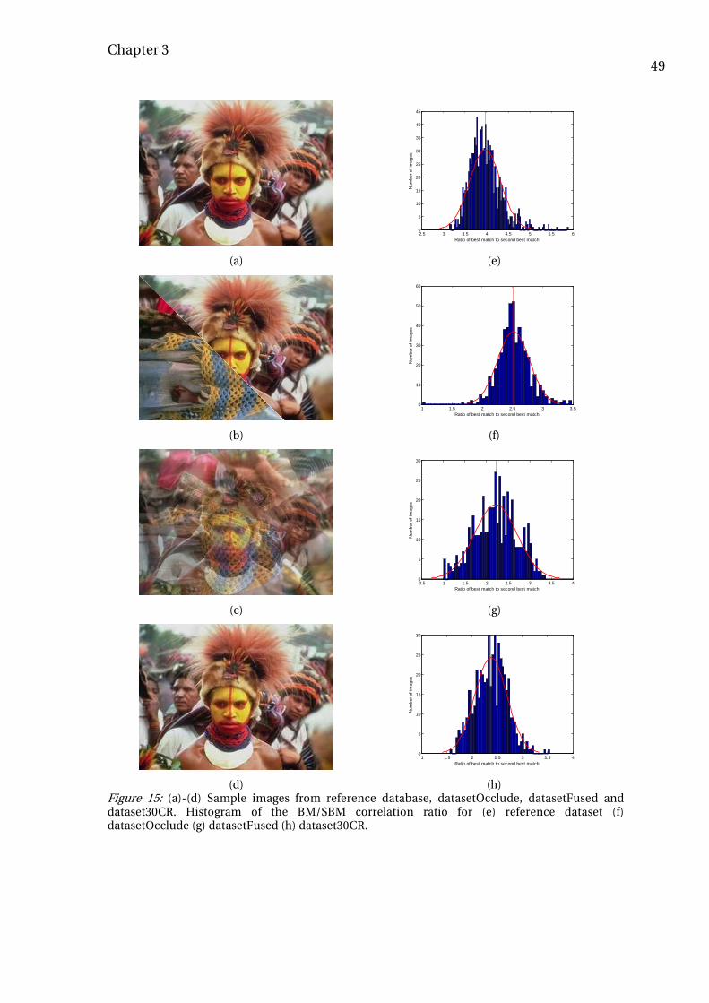
Chapter 3 49

(a) (e)

(b) (f)

(c) (g)

(d) (h) Figure 15: (a)-(d) Sample images from reference database, datasetOcclude, datasetFused and dataset30CR. Histogram of the BM/SBM correlation ratio for (e) reference dataset (f) datasetOcclude (g) datasetFused (h) dataset30CR.

2.5 3 3.5 4 4.5 5 5.5 60

5

10

15

20

25

30

35

40

45

Ratio of best match to second best match

Num

ber o

f im

ages

1 1.5 2 2.5 3 3.50

10

20

30

40

50

60

Ratio of best match to second best matchN

umbe

r of i

mag

es

0.5 1 1.5 2 2.5 3 3.5 40

5

10

15

20

25

30


Num

ber o

f im

ages

1 1.5 2 2.5 3 3.5 40

5

10

15

20

25

30


Num

ber o

f im

ages

Chapter 3 50

Figure 17, compares the maximum, the minimum and the mean of the BM/SBM correlation ratio for the proposed image retrieval algorithm and the algorithms in [62] and [61], for all datasets tests combined. We can see from the figure that the proposed algorithm using DCTPM outperforms [62] and [61].

Figure 17: Comparison of maximum, minimum, and mean of the correlation ratio of BM/SBM.

Maximum Minimum Mean0

0.5

1

1.5

2

2.5

3

3.5

4

4.5

Cor

rela

tion

ratio

of B

M/S

BM

Proposed image retrieval using DCTPMI.Ito et.alJ.Bracamonte et.al

(a) (b) (c) (d)

Figure 16: (a) Occluded image (b) Region Merging (RM) using proposed DCTPM algorithm (c) RM on [61] (d) RM on [62].

Chapter 3 51

3 Low complexity image retrieval algorithm

3.1. Introduction

As we have seen in the first chapter, low complexity image retrieval algorithms are required to perform image retrieval in handheld devices especially where the time taken to retrieve an image is paramount. In section 1 and section 2 of this chapter we have developed two different image retrieval algorithms. In this section, we see how these two algorithms can be combined in a two-stage search to obtain a low complexity image retrieval algorithm.

Two-stage search

To decrease the complexity while keeping a good performance, image retrieval is done in two stages. The first stage uses a low complexity algorithm which searches over the entire database and returns the top N images that form the closest match to the query image, which are collectively called as the pre-selected database. The first stage algorithm is fast but not very accurate, i.e., the best image returned might not correspond to the query image. However, we choose N large enough such that the query image is always contained in the pre-selected database.

In the second stage we use a more robust and accurate, but computationally more complex algorithm. This algorithm searches for the query image on the pre-selected database returned by the first stage. We can afford the increase in complexity as the number of images to be searched by the second stage algorithm is reduced to N (by the first stage).

3.2. Proposed image retrieval algorithm

The proposed image retrieval algorithm consists of three main blocks, which are shown in Figure 18 and explained as follows.

3.2.1. Border Recognition, Reconstruction and Preprocessing (BRRP)

This first block is used to align and crop the input image, i.e., the image to be recognized which is acquired with the camera, and thus subject to geometric transformations, such as rotation, scaling and translation (RST) with respect to the reference version stored in the database. The algorithms used to perform this BRRP are discussed in chapter 4.

3.2.2. Color Density Circular Crop (CDCC) Pre-selection

This second block is a pre-selection algorithm used to decrease the complexity. CDCC, is a less complex but also less robust algorithm, which searches the database and preselects the 50 images that are closest to the query image.

Chapter 3 52

CDCC uses as features the color proportions within concentric circular zones of the image, as seen in subsection 1.2. For every image stored in the database, the feature vector is pre-calculated and stored. When a query image is acquired, the feature vector of the query is calculated and compared, using L1 distance, with the feature vector of each of the images stored in the database. As the feature vector length is small and also low in complexity to compute, the CDCC algorithm is low in complexity. Additionally, this algorithm is robust to rotation, scaling, and translation, but is sensitive to variations in lighting.

3.2.3. DCT Phase Match (DCTPM)

The third block, seen in section 2, is the base recognition algorithm, which is referred to as “DCT phase match” (DCTPM). This algorithm is accurate and robust to lighting variation but computationally expensive and not RST invariant. To reduce the overall complexity of the system while keeping good accuracy, DCT phase match is only performed on the reduced database of the 50 images pre-selected by the CDCC algorithm.

Acquired Image

BRRP

CDCC Pre-selectionQuery Image

Reduced Database

DCT Phase Match (DCTPM)

JPEG images

Query Image

CDCC Features

Database

indexes

Best Match

DCTphase

Figure 18: Overview of the proposed image recognition algorithm.

Chapter 3 53

The DCTPM algorithm searches for the best match of the query image into the pre-selected database using correlation on the DCT phase of the 8 × 8 blocks of the images, and is therefore compatible with the JPEG compression standard.

The region merging method described in the DCTPM algorithm in subsection 2.2 is not used as we ignore the case of occluded images which are rejected in the BRRP stage.


In the subsections 3.3.1 and 3.3.2 we explain the databases used for experimental evaluation, the testing procedure, and the obtained results. Then, in subsection 3.3.3 the proposed algorithm is compared with popular image retrieval algorithms based on SIFT features, GIST features, and color histograms.

3.3.1. Experimental database

Two databases, one for pictograms and one for pictures, were used during the tests. The pictogram database contains 1500 pictograms from the Picture Communication Symbols set [56] The pictograms were stored in JPEG format with 85% quality, and QVGA resolution (320×240). The picture database contains the 1000 pictures of the COREL photograph database used in [57] which contains JPEG compressed color images with QVGA resolution. We refer to these two databases as the “clean pictogram database” and the “clean picture database”.

Camera Setup

To reproduce the conditions in real world, the fixed focus OV7675 camera module [58] was fixed at a distance of 9.2 cm from the image. Under this condition, a VGA resolution acquired image corresponds to a rectangle of

(a) (b)

Figure 19: (a) Example of printed pictogram with border (b) Camera setup with LED crown.

Chapter 3 54

6 × 8 cm. A subset of 50 representative pictograms and 50 representative pictures, shown in Figure 20, was selected from the 1500 pictograms and the 1000 pictures of the “clean database” and were printed on paper with a size of 3 × 4 cm. To provide a reference for alignment, a 3 × 4 cm rectangle enclosing the image was printed as shown in Figure 19(a). The 50 printed pictograms and the 50 printed pictures were then acquired with the camera, from MATLAB. These acquired images constitute respectively the “real condition pictogram database” and the “real condition picture database”.

In preliminary tests, we found that the image recognition system did not perform well with pictures. This was due to problems with color space matching under different illumination conditions for the CDCC pre-selection algorithm. To solve this problem a LED crown with a diffuser was mounted on the camera to provide uniform lighting along with a reference image to calibrate the camera for changes in color gamut (see chapter 5). The camera setup with LED crown is shown in Figure 19(b).

3.3.2. Testing procedure and results

The proposed image recognition algorithm was implemented in MATLAB. For testing, we have used the two clean databases presented in subsection 3.3.1. Every image within the database is successively used as query, running the search for this image on the entire database. Tests were also performed with different rotations of the query image at 30, 60 and 90 degrees. The recognition accuracy is calculated as the proportion of cases in which the best match corresponds to the query image, with respect to the number of trials. These tests always found the best match as the query image.

We also performed tests with the real condition databases (see subsection 3.3.1). These tests also found the query image as the best match in all the cases.

The DCTPM correlations, as seen from Eq. (28), are normalized between 1 and 0 and the correlation of the best match is 1 if the query image matches exactly with the best match. The correlation of the second (and subsequent) match measures the discrimination power of the search algorithm. Thus, lower the correlation of the second match, the higher the discrimination power.

For clean pictures, the worst-case (largest) correlation of the 2nd match is 0.316, the average is 0.247 and the best-case (smallest) is 0.156. For clean pictograms the worst-case (largest) correlation of the 2nd match is 0.972, the average is 0.216 and the best-case (smallest) is 0.099. For 96.2 % of the cases we have a correlation of the 2nd match below 0.5. The few cases with high 2nd correlation correspond to visually similar images.

Chapter 3 55

Figure 20 (a): The subset of 50 pictograms used for producing the real databases.

Chapter 3 56

Figure 20(b): The subset of 50 pictures used for producing the real databases.

Chapter 3 57

3.3.3. Comparison with other retrieval algorithms

The proposed image retrieval algorithm has been compared with other state of the art image retrieval algorithms described in chapter 2. The algorithms to which the proposed retrieval algorithm is compared are image retrieval algorithms based on Scale Invariant Feature Transform (SIFT) descriptors2 [38] [70], GIST feature descriptors [35], and global color histogram using chi-square (𝜒2) histogram distance [24].

The main advantage of our algorithm is that, since it is low in complexity, the execution time is much faster compared to the standard SIFT, GIST, or color histogram based image retrieval. Also, it is seen that SIFT is not well suited for retrieval of pictograms as they do not have enough distinct local features. Table 5 shows the comparisons of our algorithm with SIFT, GIST, and color histograms, for both clean pictogram and picture databases.

From Table 5 we can see that our algorithm outperforms SIFT, GIST, and color histograms in execution time needed to find the best match. Also, in the case of pictograms, our algorithm is better than SIFT, showing higher discrimination power and accuracy. However, for the case of pictures, the discrimination power of SIFT is higher than in our algorithm. It should be noted that in the case of GIST and color histograms the given discrimination factor is between the second and third best match (instead of between the first and the second) as the first best match is always zero and hence GIST cannot be compared directly with the discrimination factor used in our proposed algorithm and SIFT.

2 Open source VLFeat (vlfeat.org) MATLAB toolbox for SIFT implementation was used.

Chapter 3 58


An effective scheme for Content Based Image Retrieval using a low complexity image retrieval algorithm was proposed in this chapter. Two novel algorithms to perform image retrieval, ‘Color Density Circular Crop’ and ‘DCT-phase match’, were first introduced. Then, a low complexity image retrieval algorithm which uses these two algorithms in two stages was also proposed.

The proposed Color Density Circular Crop (CDCC) features are the normalized color densities within circular concentric zones in the image, encompassing the edge pixels. They are invariant to rotation, scaling, and translation. The typical size of the feature vector is small (L = 12), hence reducing the memory used and retrieval time. Further, the computational load of the

Proposed image retrieval algorithm SIFT descriptors based algorithm [38]

Average best

match/ Second

best match

Average time taken

(s)

Number of best matches

corresponding to the query

image

Average number of

keypoints in best

match/second best match

Average time

taken(s)



image

Pictograms 4.63 0.60 1500 2.8 9.15 1483

Pictures 4.05 0.60 1000 8.1 16.45 1000

Color histogram based algorithm GIST descriptors based algorithm [35]

Average Second

best match/

Third best match

Average time taken

(s)



image

Average Second best

match/ Third best match

Average time

taken(s)



image

Pictograms 1.17 6.66 1500 1.29 7.99 1500

Pictures 2.76 5.78 1000 1.27 5.52 1000

Table 5: Comparison between the proposed retrieval algorithm and SIFT, Color histogram and GIST.

Chapter 3 59

feature extraction is low. Accuracy of the CDCC algorithm is good for the system, as the query image is always found in the top 10 best matches for clean database and the top 30 best matches for real condition database.

The proposed DCT-phase based image retrieval algorithm uses a novel correlation metric for ternary-valued DCT-phase. A new region merging method was also introduced, which was used to extract the non-occluded regions from the retrieved image. The proposed DCT-phase based image retrieval method showed an average "Best Match to Second Best Match correlation ratio" of 2.96, when tested with different datasets containing reference images, occluded images, fused images, and images compressed with different JPEG compression ratios. Experimental evaluation also showed that the proposed DCT-phase based image retrieval method performs better than the current state of the art DCT-phase based image retrieval methods by at least a factor of 2.

The proposed low complexity image retrieval algorithm which uses the ‘Color Density Circular Crop’ algorithm, as the pre-selection stage, and the ‘DCT-phase match’ algorithm, as the base recognition algorithm, showed good performance under experimental evaluation. The proposed algorithm outperformed the state of the art algorithm using SIFT, GIST, and color histogram descriptors in terms of execution speed by a factor of 21.33. Moreover, the proposed algorithm had a higher accuracy for the specific case of pictogram database compared to the algorithm using SIFT descriptors. However, the proposed low complexity image retrieval algorithm requires RST compensation with respect to the reference image when using real world acquired query images. Algorithms for performing this RST compensation are discussed in detail in chapter 4.

Chapter 4

Rotation, scaling, and translation compensation algorithms

In this chapter we present the algorithms developed during the PhD work that are used for rotation, scaling, and translation (RST) compensation with respect to the reference image. In the first section of the chapter we present an algorithm, which has been published at EUSIPCO 2011 [5], that compensates for RST without using any printed references. In the second section we present two algorithms which are used to compensate for RST by using a printed reference along the border of the image. We have tested the performance of these compensation algorithms when used in conjunction with the low complexity image retrieval algorithm proposed in chapter 3.

Chapter 4 62

1 Introduction

Content Based Image Retrieval (CBIR) can be used for handheld image recognition devices in which the query image to be recognized is acquired with a camera, and thus there is no additional metadata associated to it. However, due to the camera acquisition, the query image is subject to geometric distortions, such as Rotation, Scaling and Translation (RST) with respect to the reference non-distorted version stored in the database. We had thus the need to develop compensation algorithms, suitable for real time implementation in portable devices, to correct for these geometric distortions.

We have studied two different classes of RST compensation algorithms, presented in section 2 and section 3. The first class comprises compensation without any printed reference, i.e., no special reference markers placed in the image to know its orientation. The second class of compensation algorithms uses a printed reference, placed in the image, whose orientation is known a priori. This reference is detected and used to compensate for the geometrical changes. Both compensation algorithms were implemented and tested in conjunction with the image retrieval algorithm proposed in chapter 3.

The following subsections introduce the mathematical foundation for representing image rotation, scaling, and translation. This representation helps to better understand and formulate the RST compensation algorithms which are described later in the chapter.

1.1. Mathematical representation of rotation, scaling and translation

The amount of rotation, scaling, and translation compared to the reference, non-distorted, greyscale image with pixels at positions (𝑥𝑖,𝑦𝑖) can be mathematically modeled as follows.

Rotation

The rotation operator performs a geometric transformation which maps the position (𝑥1,𝑦1) of a pixel in an input image onto the position (𝑥2,𝑦2) in an output image, by rotating it through an angle 𝜃 about the center of rotation (𝑥0,𝑦0).

𝑥2 = cos𝜃 (𝑥1 − 𝑥0) − sin𝜃 (𝑦1 − 𝑦0) + 𝑥0

𝑦2 = sin𝜃 (𝑥1 − 𝑥0) + cos 𝜃 (𝑦1 − 𝑦0) + 𝑦0

(30)

The intensity at the position (𝑥2,𝑦2) can be assigned by interpolation or averaging the intensities of the pixels in the neighborhood.

Chapter 4 63

Scaling

The scaling operator performs a geometric transformation which can be used to reduce or increase the size of an image:

𝑥2 = 𝑠 ∗ 𝑥1

𝑦2 = 𝑠 ∗ 𝑦1 (31)

where s is the scaling parameter. If 𝑠 > 1, the image size is increased and we need to assign the intensity to the intermediate positions by either replication or interpolation of the intensities of pixels in the neighborhood. If 𝑠 < 1, the image size is reduced and we need to subsample the pixel values, by replacing a group of pixel intensities by one intensity chosen from within this group or averaging intensities of neighborhood pixels.

Translation

The translation operator performs a geometric transformation which maps the position (𝑥1,𝑦1) of each pixel in an input image into a new position (𝑥2, 𝑦2) in an output image, by shifting it through a user-specified translation (∆𝑥,∆𝑦):

𝑥2 = 𝑥1 + ∆𝑥

𝑦2 = 𝑦1 + ∆𝑦 (32)

The treatment of elements near image edges varies with the implementation. Translation is used to improve visualization of an image, but also has a role as a preprocessor in applications where registration of two or more images is required.

RST transform representation

The combined Rotation, Scaling, and Translation (RST) operator can be expressed in matrix form. Consider a two-dimensional reference greyscale image 𝑓 and the corresponding RST transformed image 𝑓𝑅𝑆𝑇 which are related by the transformation 𝑓𝑅𝑆𝑇 = 𝑇(𝑓). The relation of each pixel 𝑓 (𝑥,𝑦) of 𝑓 that maps to a corresponding pixel 𝑓𝑅𝑆𝑇(𝑥𝑡,𝑦𝑡) of 𝑓𝑅𝑆𝑇 is given by:

�𝑥𝑡𝑦𝑡1� = �

𝑠 𝑐𝑜𝑠𝜃 −𝑠 𝑠𝑖𝑛𝜃 𝛥𝑥𝑠 𝑠𝑖𝑛𝜃 𝑠 𝑐𝑜𝑠𝜃 𝛥𝑦

0 0 1� �𝑥𝑦1� (33)

where the RST parameters are the rotation angle (𝜃), the scaling parameter (s), and the translation parameter (𝛥x, 𝛥y).

Chapter 4 64

2 RST compensation without printed reference

We have first developed an algorithm that performs RST compensation without any printed reference. The algorithm automatically extracts the RST parameters, between the reference image and the transformed image.

This RST parameter extraction is based on the Fourier-Mellin Transform, explained in subsection 2.1, for which we propose, in subsection 2.2, an efficient implementation using log-polar grid interpolation, with experimental evaluation given in subsection 2.3.

2.1. Fourier-Mellin transform

The optical research community introduced the Fourier-Mellin Transform (FMT) for pattern recognition [71, 72] which was later used in digital signal and image processing [73, 74]. FMT for image recognition was initially reported by Chen et al. [75] and used to extract RST invariant features. In recent years we have seen an increased use of FMT for extracting RST invariant features [76, 77].

The FMT is a useful mathematical tool for image recognition because its resulting spectrum is invariant in rotation, scaling, and translation. The Fourier Transform (FT) itself is translation invariant and its conversion to log-polar coordinates converts the scaling and rotation differences to vertical and horizontal offsets that can be measured. A second FFT, called the Mellin transform (MT) gives a transform-space image that is invariant to translation, rotation, and scaling. FMT is frequently used in content-based image retrieval and digital image watermarking.

Fourier-Mellin Transform is used to extract the RST parameters which are then used to compensate the query image before comparing it using image matching algorithms. The RST parameters are the rotation angle (𝜃), the scaling parameter (s), and the translation parameter (𝛥x, 𝛥y) as seen in the previous section. From Eq.(33), the transformed pixel 𝑓𝑅𝑆𝑇(𝑥𝑡,𝑦𝑡) can be rewritten as:

𝑓𝑅𝑆𝑇(𝑥𝑡,𝑦𝑡) = 𝑓(𝑠 ∙ (𝑥 ∙ 𝑐𝑜𝑠𝜃 − 𝑦 ∙ 𝑠𝑖𝑛𝜃) + ∆𝑥, 𝑠 ∙ (𝑥 ∙ 𝑠𝑖𝑛𝜃 + 𝑦 ∙ 𝑐𝑜𝑠𝜃) + ∆𝑦) (34)

taking the Fourier transform of the Eq.(34), we have:

Ӻ𝑅𝑆𝑇(𝑢, 𝑣) =𝑒−𝑗2𝜋(∆𝑥∙𝑢+∆𝑦∙𝑣)

𝑠2∙ Ӻ �

𝑢 ∙ 𝑐𝑜𝑠𝜃 − 𝑣 ∙ 𝑠𝑖𝑛𝜃𝑠

,𝑢 ∙ 𝑠𝑖𝑛𝜃 + 𝑣 ∙ 𝑐𝑜𝑠𝜃

𝑠� (35)

where Ӻ and Ӻ𝑅𝑆𝑇 are the Fourier transform of 𝑓 and 𝑓𝑅𝑆𝑇, respectively. Mapping to log-polar domain using 𝑢 = 𝑒𝜌𝑐𝑜𝑠𝜑 and 𝑣 = 𝑒𝜌𝑠𝑖𝑛𝜑, and taking the magnitude of

Chapter 4 65

both sides of the equation, we have, from the translation and scaling property of Fourier transform:

|Ӻ𝑅𝑆𝑇(𝑒𝜌𝑐𝑜𝑠𝜑, 𝑒𝜌𝑠𝑖𝑛𝜑)| =1𝑠2 �

Ӻ �𝑒𝜌−𝑙𝑜𝑔 𝑠𝑐𝑜𝑠(𝜃 + 𝜑), 𝑒𝜌−𝑙𝑜𝑔 𝑠𝑠𝑖𝑛(𝜃 + 𝜑)�� (36)

Ӻ𝑅𝑆𝑇−𝐿𝑃(𝜌,𝜑) =1𝑠2Ӻ𝐿𝑃(𝜌 − 𝑙𝑜𝑔 𝑠,𝜃 + 𝜑) (37)

where Ӻ𝑅𝑆𝑇−𝐿𝑃 and Ӻ𝐿𝑃 are the log-polar mapping of |Ӻ𝑅𝑆𝑇| and |Ӻ| respectively.

From Eq.(37) we can see that the rotation (by 𝜃) and the scale (by s) are now translations in the mapped domain, and we can measure this rotation (𝜃) and scaling (s) by performing a 2D phase correlation [78] using the translation property of the Fourier transform:

𝑓2(𝑥,𝑦) = 𝑓1(𝑥 − 𝑥0,𝑦 − 𝑦0)

(38)

Ӻ1(𝜉, 𝜂)Ӻ2∗(𝜉, 𝜂)

|Ӻ1(𝜉, 𝜂)Ӻ2∗(𝜉, 𝜂)| = 𝑒𝑗2𝜋(𝜉𝑥0+𝜂𝑦0)

After the rotation and scaling parameters are extracted we compensate the image for these extracted parameters and then run another 2D phase correlation to extract the translation parameter (𝛥x, 𝛥y).

2.2. Implementation of Fourier-Mellin transform

To efficiently implement Fourier-Mellin transform for extracting the RST compensation parameters, we implement the log-polar mapping seen in the previous subsection by using log-polar grid interpolation (see subsection 2.2.1).

Figure 21 shows an example of the RST parameters extraction and compensation using FMT. Figure 22 shows the flowchart for the implementation of the algorithm which has the following steps:

1. Calculate the Fourier transform of the query image and the candidate reference image from the database and shift the zero-frequency component to the center of the spectrum.

2. Perform band-pass filtering with a minimum radius of ρmin and maximum radius ρmax., and then log-polar mapping of the magnitude of the Fourier transform. The radii ρmin and ρmax are calculated as 0.04 and 0.8 times of the minimum distance from the center of the image to the end of the frame.

3. Perform phase correlation between the two log-polar mapped images, and extract the rotation (𝜃) and scaling (s) parameters.

Chapter 4 66

4. Compensate the query image for rotation and scaling, using the extracted rotation and scaling parameters.

5. Perform phase correlation on the compensated query image with respect to the reference image to extract the translation parameters (𝛥x, 𝛥y).

6. Compensate the query image (already corrected for rotation and scaling) for translation, using the extracted translation parameters.

2.2.1. Log-polar grid interpolation

The log-polar grid is obtained by quantizing the two parameters of Eq. (37), which are the radius, 𝜌, and the angle, 𝜑. The radius is quantized by dividing logarithmically the distance from the center of the image (𝑥𝑐,𝑦𝑐) to the corner of

(a) (c) (e) (g)

(b) (d) (f) (h)

(i) (j) (k)

Figure 21: (a) Reference image; (b) Rotated and scaled image; (c),(d) Center-shifted Fourier transform of (a) and (b) respectively; (e),(f) Band-pass filtered version of (c) and (d); (g),(h) Log-polar mapping of (e) and (f); (i) Log-polar mapping grid; (j) Phase correlation between (g) and (h); (k) RST compensated image.

Chapter 4 67

the image. The angle is linearly quantized between 0 and 2π. That is, in MATLAB commands:

ρ = logspace(0,log(d))

φ = linspace(0,2π)

The amount of points in the log-polar grid is chosen according to the resolution of the image, so as to have the same amount of points as in the sampling grid of the frequencies of the image (𝑢, 𝑣) of Eq. (35).

By using FFT, we have already calculated the value of the transforms at all the points of the (𝑢, 𝑣) sampling grid. In order to calculate the values of the transforms at the points of the (𝜌,𝜑) log-polar grid we proceed as follows. We first map the points of the (𝑢, 𝑣) sampling grid into points in the (𝜌,𝜑) log-polar domain. We then know the value of the transforms at these points, but these points are not necessary on the (𝜌,𝜑) log-polar grid. We thus obtain the values for each point of the log-polar grid by linear interpolation using the known values of neighboring points of the mapped (𝑢, 𝑣) grid.

Figure 23 shows an example of a log-polar grid which has been filtered with a band pass filter with a minimum radius of 𝜌𝑚𝑖𝑛 and maximum radius 𝜌𝑚𝑎𝑥. The grid points are at the intersection of the radial lines with the concentric circles. The actual log-polar grid we have used is shown in Figure 21(i).

Fourier transform

Filter and Log-Polar Mapping

Correct image for scale & angle

Phase Correlation

Phase correlation

Correct image for translation

Query Image Reference Image

θ s

(∆x,∆y)

Figure 22: Fourier-Mellin transform implementation for RST compensation.

Chapter 4 68


We evaluate the proposed RST compensation method when used in conjunction with the two-stage low complexity image retrieval algorithm proposed in chapter 3. The second stage of this algorithm uses DCT phase matching which is sensitive to geometrical variations like rotation, scaling, and translation. We thus compensate the images for these RST variations before performing DCT phase matching. A block diagram of the setup is shown in Figure 24.

In the next sub-sections we explain the databases used for experimental evaluation, the testing procedure, and the obtained results.

2.3.1. Test databases

Two databases, one for pictograms and one for pictures were used during the tests. The pictogram database contains 1500 pictograms from the Picture Communication Symbols (PCS) set [56]. The pictograms were stored in JPEG format with 85% quality, and QVGA resolution (320 x 240). The picture database contains the 1000 pictures from the COREL photograph data set used in [57] which are also JPEG compressed color images with QVGA resolution. We refer to these two databases as the "clean pictogram database" and the "clean picture database".

𝜌m

ax

φn

π φ = 0𝜌min

(xc,yc)

Figure 23: Log-polar mapping grid with logarithmically spaced radii (𝜌) and linearly spaced angles (𝜑) with center(𝑥𝑐 , 𝑦𝑐).

Chapter 4 69

Additionally, a set of 50 representative pictograms and 50 representative pictures were chosen from the clean databases. These images were printed and acquired using a fixed focus OV7675 VGA camera from OmniVision [58]. These two sets of 50 images constitute what we call the "real condition pictogram database" and the "real condition picture database".


The proposed image recognition system with RST compensation was implemented in MATLAB. For testing, we have used the two clean databases presented in subsection 2.3.1. Every image within the database is successively used as query, running the search for this image on the entire database. With each query image, we run seven searches, each with different conditions: no RST, rotation by an angle 𝜃 of 30, 60 and 90 degrees, scaling by a factor 𝑠 of 0.5 and 0.75, and translation by (∆𝑥,∆𝑦) = (100,100). A similar test is done with the two real condition databases, with no RST.

(∆𝑥,∆𝑦)

Acquired Image

CDCC Pre-selectionQuery Image

Reduced Database


JPEG imagesQuery Image

CDCC Features

Database

indexes

Best Match

Extract RST using FMT

Correct Query for RST𝜃 s

DCT phase

Figure 24: Overview of the proposed image recognition algorithm with RST compensation using Fourier-Mellin transform.

Chapter 4 70

2.3.3. Test results

Table 6 summarizes the results of the testing procedure. The recognition accuracy is calculated as the proportion of cases in which the best match corresponds to the query image, with respect to the number of trials. We can see that for clean database and no RST transformations, the system has 100% accuracy.

The average accuracy in case of rotation by an angle θ of 30, 60 and 90 degrees is 96.0 % for pictograms and 97.9 % for pictures. Similarly the average accuracy for scaling, by a factor of 0.5 and 0.75, is 89.8 % for pictograms and 93.1 % for pictures. We can see from the above results that the system performs slightly better for pictures than for pictograms, as pictures have more spectral information than pictograms, which is used in the FMT based RST compensation and in DCT phase matching. The reduction in recognition accuracy compared to no RST transformed images, is from the tolerances of FMT compensation which are passed on to DCT phase matching stage which is sensitive to RST variations.

With the real condition database, where the pictograms and pictures are acquired from the camera, the accuracy is 90% for pictograms and 94% for pictures.

Initial development was done using FMT for RST compensation, but later the solution with a rectangular border (explained in the next section) was found to be more robust and should be used wherever possible. In a case where imposing a printed rectangular border is not feasible, we can align the images using Fourier-Mellin Transform.

3 RST compensation with printed reference

In the previous section we have seen an RST compensation algorithm that can be used in the case where it is not feasible to impose a printed reference on the images to be recognized. In this section we study RST compensation algorithms using a printed pattern as a reference to improve robustness of the image recognition system. The printed pattern we consider is a rectangular border added around the image.

Chapter 4 71

Two different algorithms, explained in subsections 3.1 and 3.2, are proposed for rectangle detection, one based on line detection using Hough transform and the other based on corner detection. After the rectangular border is detected with either of the two proposed algorithms, we correct the orientation of this rectangle for any RST variations by using perspective transform, as explained in subsection 3.3. The two resulting RST compensation algorithms were implemented and tested in conjunction with the image retrieval algorithm proposed in chapter 3. This experimental evaluation is given in subsection 3.4.

3.1. Line detection

A rectangle can be described by means of its sides. They can be detected with the help of a straight line extraction procedure such as template matching [79]. For rectangle detection, the use of a straight line as the basic unit is more effective in comparison to pixel as the basic unit, as suggested in [80]. In this

Pictograms Pictures

Cle

an d

atab

ase

No RST 100% 100%

Rotation

𝜃 = 30° 93.93% 96.8%

𝜃 = 60° 94.6% 97.2%

𝜃 = 90° 99.6% 99.8%

Scaling s = 0.5 88.46% 90.7%

s = 0.75 91.13% 95.4%

Translation(∆𝑥,∆𝑦) =(100,100)

99.06% 98.9%

Real condition database 90% 94%

Table 6: Summary of results from the image recognition system for ‘real condition database’ and under different RST conditions on ‘clean database’.

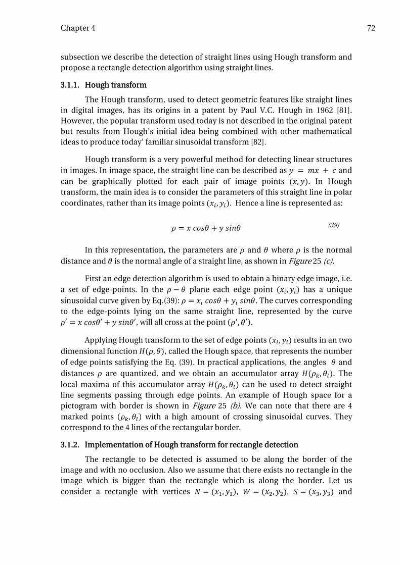
Chapter 4 72

subsection we describe the detection of straight lines using Hough transform and propose a rectangle detection algorithm using straight lines.

3.1.1. Hough transform

The Hough transform, used to detect geometric features like straight lines in digital images, has its origins in a patent by Paul V.C. Hough in 1962 [81]. However, the popular transform used today is not described in the original patent but results from Hough’s initial idea being combined with other mathematical ideas to produce today’ familiar sinusoidal transform [82].

Hough transform is a very powerful method for detecting linear structures in images. In image space, the straight line can be described as 𝑦 = 𝑚𝑥 + 𝑐 and can be graphically plotted for each pair of image points (𝑥, 𝑦). In Hough transform, the main idea is to consider the parameters of this straight line in polar coordinates, rather than its image points (𝑥𝑖,𝑦𝑖). Hence a line is represented as:

𝜌 = 𝑥 𝑐𝑜𝑠𝜃 + 𝑦 𝑠𝑖𝑛𝜃 (39)

In this representation, the parameters are 𝜌 and 𝜃 where 𝜌 is the normal distance and 𝜃 is the normal angle of a straight line, as shown in Figure 25 (c).

First an edge detection algorithm is used to obtain a binary edge image, i.e. a set of edge-points. In the 𝜌 − 𝜃 plane each edge point (𝑥𝑖, 𝑦𝑖) has a unique sinusoidal curve given by Eq.(39): 𝜌 = 𝑥𝑖 𝑐𝑜𝑠𝜃 + 𝑦𝑖 𝑠𝑖𝑛𝜃. The curves corresponding to the edge-points lying on the same straight line, represented by the curve 𝜌′ = 𝑥 𝑐𝑜𝑠𝜃′ + 𝑦 𝑠𝑖𝑛𝜃′, will all cross at the point (𝜌′,𝜃′).

Applying Hough transform to the set of edge points (𝑥𝑖 ,𝑦𝑖) results in an two dimensional function 𝐻(𝜌,𝜃), called the Hough space, that represents the number of edge points satisfying the Eq. (39). In practical applications, the angles 𝜃 and distances 𝜌 are quantized, and we obtain an accumulator array 𝐻(𝜌𝑘,𝜃𝑙). The local maxima of this accumulator array 𝐻(𝜌𝑘,𝜃𝑙) can be used to detect straight line segments passing through edge points. An example of Hough space for a pictogram with border is shown in Figure 25 (b). We can note that there are 4 marked points (𝜌𝑘,𝜃𝑙) with a high amount of crossing sinusoidal curves. They correspond to the 4 lines of the rectangular border.

3.1.2. Implementation of Hough transform for rectangle detection

The rectangle to be detected is assumed to be along the border of the image and with no occlusion. Also we assume that there exists no rectangle in the image which is bigger than the rectangle which is along the border. Let us consider a rectangle with vertices 𝑁 = (𝑥1,𝑦1), 𝑊 = (𝑥2,𝑦2), 𝑆 = (𝑥3,𝑦3) and

Chapter 4 73

𝐸 = (𝑥4,𝑦4). 𝑁𝑊 and 𝑆𝐸 are parallel sides of the rectangle with length 𝑎 and 𝑊𝑆 and 𝐸𝑁 are parallel sides with length 𝑏.

The algorithm for detection of the four vertices of the rectangle using Hough transform is as follows:

1. Compute the edges-points in the image using a canny edge detector [55].

2. Quantize the parameter space in 𝜌 (∈ [0,�(𝑊2 + 𝐻2)] ; where the image is of

size 𝑊 x 𝐻) and in 𝜃 (∈ �−𝜋2

, 𝜋2�).

3. Form a 𝑛-dimensional accumulator array 𝐻(𝜌𝑘,𝜃𝑙), with structure matching the quantization of the parameter space; set all elements to zero.

4. For each edge point (𝑥𝑖,𝑦𝑖) in the edge image, increase the accumulator cells 𝐻(𝜌𝑘,𝜃𝑙) such that

FOR 𝜃𝑙 = 𝜃𝑚𝑖𝑛UNTIL 𝜃𝑙 ≤ 𝜃𝑚𝑎𝑥 CALCULATE 𝜌𝑘 = 𝑥 𝑐𝑜𝑠𝜃𝑙 + 𝑦 𝑠𝑖𝑛𝜃𝑙 and INCREMENT 𝐻(𝜌𝑘,𝜃𝑙)

5. Find the local maxima of the accumulator cell 𝐻(𝜌𝑘,𝜃𝑙) which gives the presence of the line.

6. Look if the lines meet each other at 90 degrees (with ±3 degrees of tolerance) and if their intersections follow the specific dimensions of length 𝑎 and 𝑏, so that a rectangle can be formed from these lines.

7. Mark the points of intersection, which form the rectangle, as 𝑁(orth), 𝑆(outh), 𝐸(ast) and 𝑊(est), where the distance between 𝑁(orth) and 𝑊(est) points corresponds to the smaller side (𝑚𝑖𝑛{𝑎, 𝑏}) of the rectangle.

3.2. Corner detection

It is advantageous to find the interest points of the reference pattern (rectangle in our case) such as corners when considering geometric transformations. Knowing the position of the corresponding points enables the estimation of parameters describing geometric transforms.

A corner in the image can be defined as a pixel having in its small neighborhood two dominant and different edge directions. This definition is not precise because other image points, such as an isolated point of local intensity maximum or minimum, a line ending, or an abrupt change in the curvature of a curve, can present this condition. Nevertheless, detectors for this condition are named corner detectors in literature and widely used. Corners in images can be located using local detectors; input to the corner detector is the gray-level image, and output is the image in which values are proportional to the likelihood that the pixel is a corner. Corners serve better than lines when solving due to their lower computational complexity. However, corner detectors are not usually very robust.

Chapter 4 74

This deficiency is overcome by having two stages, using two different algorithms, one for detection of corners and another for verification of the corners found. For detection we use Harris corner detector algorithm [83] and for verifying if the corner detected is a valid corner, we use a modified variant of “Smallest Univalue Segment Assimilating Nucleus” (SUSAN) [84] algorithm. These two algorithms are described in subsections 3.2.1 and 3.2.2. Then, in subsection 3.2.3, we propose their efficient implementation into a rectangle detection algorithm.

3.2.1. Harris corner detector [83]

Consider a 2D grayscale image 𝑓. An image patch 𝑊 ∈ 𝑓 is taken and is shifted by (∆𝑥,∆𝑦). The sum of square differences, 𝑆, between values of the image 𝑓 in the patch 𝑊 and its shifted version is given by:

(a) (b)

ρ

θ X

Y

(x,y)

(c)

Figure 25: (a) An example pictogram with a rectangular border; (b) Hough space of the example pictogram showing the four maximum points corresponding to four lines of the rectangle; (c) Representation of a straight line in Hough parameters 𝜌 and 𝜃.

Chapter 4 75

𝑆𝑊(∆𝑥,∆𝑦) = � � (𝑓(𝑥𝑖,𝑦𝑖) − 𝑓(𝑥𝑖 − ∆𝑥,𝑦𝑖 − ∆𝑦))2𝑦𝑖∈𝑊𝑥𝑖∈𝑊

(40)

A corner point must have a high response of 𝑆𝑊(∆𝑥,∆𝑦) for all (∆𝑥,∆𝑦). If the shifted image patch is approximated by the first-order Taylor expansion

𝑓(𝑥𝑖 − ∆𝑥,𝑦𝑖 − ∆𝑦)~𝑓(𝑥𝑖,𝑦𝑖) + �𝜕𝑓(𝑥𝑖,𝑦𝑖)

𝜕𝑥𝜕𝑓(𝑥𝑖, 𝑦𝑖)

𝜕𝑦� �∆𝑥∆𝑦�

(41)

then the minimum of 𝑆𝑊(∆𝑥,∆𝑦) can be obtained analytically by substituting this approximation given by Eq.(41) into Eq.(40)

𝑆𝑊(∆𝑥,∆𝑦) = � � ��𝜕𝑓(𝑥𝑖,𝑦𝑖)


𝜕𝑦� �∆𝑥∆𝑦��

2

𝑦𝑖∈𝑊𝑥𝑖∈𝑊

(42) = [∆𝑥 ∆𝑦]

⎝

⎛� �

⎣⎢⎢⎡𝜕𝑓𝜕𝑥𝜕𝑓𝜕𝑦⎦⎥⎥⎤�𝜕𝑓𝜕𝑥

𝜕𝑓𝜕𝑦�

𝑦𝑖∈𝑊𝑥𝑖∈𝑊 ⎠

⎞�∆𝑥∆𝑦�

= [∆𝑥 ∆𝑦]𝐴𝑊(𝑥,𝑦) �∆𝑥∆𝑦�

where the Harris matrix 𝐴𝑊(𝑥, 𝑦) is the second derivative of 𝑆 around the point (𝑥,𝑦) = (0,0):

𝐴𝑊(𝑥,𝑦) =

⎣⎢⎢⎢⎢⎡ � �

𝜕2𝑓(𝑥𝑖,𝑦𝑖)𝜕𝑥2

𝑦𝑖∈𝑊𝑥𝑖∈𝑊

� �𝜕𝑓(𝑥𝑖,𝑦𝑖)

𝜕𝑥𝜕𝑓(𝑥𝑖,𝑦𝑖)

𝜕𝑦𝑦𝑖∈𝑊𝑥𝑖∈𝑊

� �𝜕𝑓(𝑥𝑖,𝑦𝑖)


𝜕𝑦𝑦𝑖∈𝑊𝑥𝑖∈𝑊

� �𝜕2𝑓(𝑥𝑖,𝑦𝑖)

𝜕𝑦2𝑦𝑖∈𝑊𝑥𝑖∈𝑊 ⎦

⎥⎥⎥⎥⎤

(43)

Usually an isotropic weighting window such as a Gaussian is used which results in an isotropic response. The Harris matrix 𝐴𝑊 represents the neighborhood, and is symmetric and positive semi-definite. Its main modes of variation correspond to partial derivatives in orthogonal directions and are reflected in the eigenvalues 𝜆1, 𝜆2of the matrix 𝐴𝑊. These modes of variations can be found using Principal Component Analysis (PCA) [85] and three distinct cases can appear:

1. Both eigenvalues 𝜆1 and 𝜆2 are small. This means that the image 𝑓 has no features of interest around the examined pixel. There are no edges or corners in this location.

Chapter 4 76

2. One eigenvalue is small and the second one is large then an edge is found. 3. Both eigenvalues are rather large. A small shift in any direction causes

significant change in image 𝑓. A corner is found.

Harris [83] suggested that the exact eigenvalue computation can be avoided by calculating the response function:

𝑅(𝐴𝑊) = 𝑑𝑒𝑡(𝐴𝑊) − 𝜅 𝑡𝑟𝑎𝑐𝑒2(𝐴𝑊) (44)

where 𝑑𝑒𝑡(𝐴𝑊) is the determinant of the local structure matrix 𝐴𝑊, 𝑡𝑟𝑎𝑐𝑒(𝐴𝑊)is the trace of matrix 𝐴𝑊, and 𝜅 is a tunable parameter, normally taking values between 0.04 to 0.15.

The main advantages of Harris corner detector are its insensitivity to 2D shift and rotation, to small illumination variations, to small viewpoint changes, and its low computational requirements compared to Hough transform.

3.2.2. Smallest Univalue Segment Assimilating Nucleus (SUSAN)

Smallest Univalue Segment Assimilating Nucleus or in short SUSAN, is a corner detection algorithm initially developed by S. M. Smith and J. M. Brady [84]. We use SUSAN algorithm to verify if the corner detected from the Harris corner detector is a true corner, because Harris corner detector can return false positives especially with noisy images.

A circular mask having a center pixel called the nucleus is shown in Figure 26 at five different positions on a binary image. If the intensity value of each pixel within a mask is compared with the intensity value of the mask’s nucleus then an area of the mask can be defined which has the same intensity value as the nucleus. This area of the mask is known as the “USAN”, an acronym standing for “Univalue Segment Assimilating Nucleus”. In Figure 26(b) each mask from Figure 26(a) is depicted with its USAN shown in white. This concept of each image point associated with a local area of similar brightness is the basis for the SUSAN principle [84].

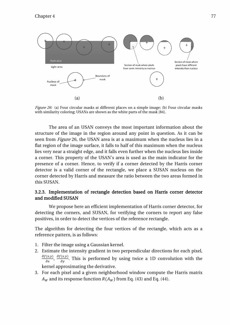
Chapter 4 77

The area of an USAN conveys the most important information about the structure of the image in the region around any point in question. As it can be seen from Figure 26, the USAN area is at a maximum when the nucleus lies in a flat region of the image surface, it falls to half of this maximum when the nucleus lies very near a straight edge, and it falls even further when the nucleus lies inside a corner. This property of the USAN’s area is used as the main indicator for the presence of a corner. Hence, to verify if a corner detected by the Harris corner detector is a valid corner of the rectangle, we place a SUSAN nucleus on the corner detected by Harris and measure the ratio between the two areas formed in this SUSAN.

3.2.3. Implementation of rectangle detection based on Harris corner detector and modified SUSAN

We propose here an efficient implementation of Harris corner detector, for detecting the corners, and SUSAN, for verifying the corners to report any false positives, in order to detect the vertices of the reference rectangle.

The algorithm for detecting the four vertices of the rectangle, which acts as a reference pattern, is as follows:

1. Filter the image using a Gaussian kernel. 2. Estimate the intensity gradient in two perpendicular directions for each pixel,

𝜕𝑓(𝑥,𝑦)𝜕𝑥

, 𝜕𝑓(𝑥,𝑦)𝜕𝑦

. This is performed by using twice a 1D convolution with the

kernel approximating the derivative. 3. For each pixel and a given neighborhood window compute the Harris matrix

𝐴𝑊 and its response function 𝑅(𝐴𝑊) from Eq. (43) and Eq. (44).

(a) (b)

Figure 26: (a) Four circular masks at different places on a simple image; (b) Four circular masks with similarity coloring; USANs are shown as the white parts of the mask [84].

Chapter 4 78

4. Choose the best candidates for corners by applying a threshold on the response function 𝑅(𝐴𝑊) and perform non-maximum suppression to find all the corners in the image.

5. Isolate the corner points which form the four vertices of the rectangle assuming the rectangle is the outer most structure in the image. i.e., find corner points that form the extrema points i.e., corner points which lie closest and farthest from the X and Y axis.

6. Verify using SUSAN if the extrema points detected are not false positives. i.e., verify that the ratio of the different areas of the USAN is within a certain threshold.

7. Mark the four corner points or vertices of the rectangle as 𝑁(orth), 𝑆(outh), 𝐸(ast) and 𝑊(est).

8. Measure the distance between these points and if needed correct the naming of the points such that the distance between the corner points 𝑁(orth) and 𝑊(est) corresponds to the smaller side (width) of the rectangle.

3.3. Perspective transform for RST compensation

Perspective transform [86] maps one arbitrary 2D quadrilateral into another. We use this transform to compensate for RST variations, after doing rectangle detection using either the line detection or the corner detection algorithms presented previously. In our case perspective transform is used to map the coordinates of the four corners of the first, recognized, rectangle (world plane coordinates) to the coordinates of the four corners of the second, RST compensated, rectangle (image plane coordinates).

A generalized camera model, which consists of central projections specialized to planes, can be written as 𝑋 = 𝐻𝑥, where the image plane coordinates are represented by lower case vectors 𝑥 = (𝑥, 𝑦, 1)𝑇, the world plane coordinates are represented by upper case vectors 𝑋 = (𝑋,𝑌, 1)𝑇, and 𝐻 is a 3 × 3 homogeneous matrix transform. Figure 27 shows the plane camera model. We can rewrite the camera model as:

�𝑋𝑊𝑌𝑊𝑊

� = �𝑎 𝑏 𝑐𝑑 𝑒 𝑓𝑔 ℎ 1

� �𝑥𝑦1� (45)

where 𝑊 = 𝑔𝑥 + ℎ𝑦 + 1. As we can see, Eq.(45) is a more generalized version of the RST transform representation given in Eq.(33). Rewriting Eq.(45) into the non-vector form of the perspective transform we have:

Chapter 4 79

𝑋 = 𝑎𝑥 + 𝑏𝑦 + 𝑐𝑔𝑥 + ℎ𝑦 + 1

𝑌 = 𝑑𝑥 + 𝑒𝑦 + 𝑓𝑔𝑥 + ℎ𝑦 + 1

(46)

To solve the above Eq.(46) for the unknown variables 𝑎, 𝑏, 𝑐,𝑑, 𝑒,𝑓,𝑔 and ℎ; we need a minimum of four points which map from the image plane (𝑥,𝑦) to the world plane(𝑋,𝑌). We can then represent Eq.(46) using the matrix form:

⎣⎢⎢⎢⎢⎢⎢⎡𝑥1 𝑦1 1 0 0 0 −𝑋1𝑥1 −𝑋1𝑦10 0 0 𝑥1 𝑦1 1 −𝑌1𝑥1 −𝑌1𝑦1𝑥2 𝑦2 1 0 0 0 −𝑋2𝑥2 −𝑋2𝑦20 0 0 𝑥2 𝑦2 1 −𝑌2𝑥2 −𝑌2𝑦2𝑥3 𝑦3 1 0 0 0 −𝑋3𝑥3 −𝑋3𝑦30 0 0 𝑥3 𝑦3 1 −𝑌3𝑥3 −𝑌3𝑦3𝑥4 𝑦4 1 0 0 0 −𝑋4𝑥4 −𝑋4𝑦40 0 0 𝑥4 𝑦4 1 −𝑌4𝑥4 −𝑌4𝑦4⎦

⎥⎥⎥⎥⎥⎥⎤

⎣⎢⎢⎢⎢⎢⎡𝑎𝑏𝑐𝑑𝑒𝑓𝑔ℎ⎦⎥⎥⎥⎥⎥⎤

=

⎣⎢⎢⎢⎢⎢⎡𝑋1𝑌1𝑋2𝑌2𝑋3𝑌3𝑋4𝑌4⎦⎥⎥⎥⎥⎥⎤

(47)

here the coordinates {(𝑥1,𝑦1), (𝑥2, 𝑦2), (𝑥3,𝑦3), (𝑥4,𝑦4)} represent the four corners of the rectangle in the image plane and {(𝑋1,𝑌1), (𝑋2,𝑌2), (𝑋3,𝑌3), (𝑋4,𝑌4)} represent the four corners or vertices of the rectangle in the world plane.

Figure 27: Camera model for perspective transform showing a point X on the world plane imaged as x in the image plane. Euclidean coordinates X-Y and x-y are used for world and image planes respectively.

Chapter 4 80

3.3.1. Implementation of RST compensation

The form of Eq.(47) is 𝐴𝜆 = 𝐵, and it can be solved by several methods that amount to a least squares estimation of the parameter vector 𝜆 that satisfies the linear relationship between the matrix A and the vector of coordinates B. One such method is by using a pseudo-inverse:

𝜆 = (𝐴𝑇𝐴)−1𝐴𝑇𝐵 (48)

The algorithm for compensation for RST parameters is as follows:

1. Map the rectangle vertices N(orth), S(outh), E(ast) and W(est) detected by either line detection or corner detection methods to points (𝑥1,𝑦1), (𝑥2, 𝑦2), (𝑥3,𝑦3) and (𝑥4, 𝑦4).

2. Map the fixed points to which rectangle has to be mapped to (𝑋1,𝑌1), (𝑋2,𝑌2), (𝑋3,𝑌3) and (𝑋4,𝑌4).

3. Compute the parameters 𝑎, 𝑏, 𝑐,𝑑, 𝑒,𝑓,𝑔, and ℎ of the homogeneous matrix transform 𝐻 using Eq.(48).

4. Map all the points in the geometrically distorted image plane (𝑥, 𝑦) into the RST compensated world plane (𝑋,𝑌) using Eq.(46).

5. Interpolate the pixel values which are missing after the transformation. The 180-degree rotated version of the images cannot be detected and

corrected in the BRRP block (as the rectangle which is rotated by 180 degrees is same as the non-rotated rectangle), and it is thus tested in the DCTPM block by correlating the DCT phase of the query image with the DCT phase of the 50 images in the reduced database and its 180-degree rotated version.


In chapter 3 we have proposed a two-stage low-complexity image retrieval algorithm which is sensitive to geometrical variations like rotation, scaling, and translation. We thus need to compensate the images for these RST variations. We evaluate the RST compensation algorithms using printed reference in conjunction with the proposed image recognition system. We refer to this RST compensation as the “Border Recognition, Reconstruction and Preprocessing” (BRRP) block which is used to align and crop the input “query image”, i.e., the image to be recognized which is acquired with the camera. A block diagram of the experimental setup is shown in Figure 18 of chapter 3.

In the next sub-sections we explain the databases used for the experimental evaluation, the testing procedure and the obtained results.

Chapter 4 81

3.4.1. Test databases

Two databases, one for pictograms and one for pictures were used during the tests. The pictogram database contains 1500 pictograms from the Picture Communication Symbols (PCS) set [56]. The pictograms were stored in JPEG format with 85% quality, and QVGA resolution (320 x 240). The picture database contains the 1000 pictures from the COREL photograph data set used in [57] which are also JPEG compressed color images with QVGA resolution. A rectangular border of 5 pixels line-width was added around the images. We refer to these two databases as the "clean pictogram database" and the "clean picture database". Figure 28 shows an example of a pictogram and a picture with a border.

Additionally, a set of 50 representative pictograms and 50 representative pictures were chosen from the clean databases. These images were printed along with the added border and acquired using a fixed focus OV7675 VGA camera from OmniVision. These two sets of 50 images constitute what we call the "real condition pictogram database" and the "real condition picture database".


The proposed image recognition system was implemented in MATLAB along with the two different RST compensation algorithms using either line or corner detection. For testing, we have used the two clean databases presented in subsection 3.4.1. Every image within the database is successively used as query, running the search for this image on the entire database. With each query image, we run seven searches, each with different conditions: no RST, rotation by an

(a) (b)

Figure 28: (a) Example of a picture with a rectangular border added as reference; (b) Example of a pictogram with a rectangular border.

Chapter 4 82

angle 𝜃 of 30, 60 and 90 degrees, scaling by a factor 𝑠 of 0.5 and 0.75, and translation by (∆𝑥,∆𝑦) = (100,100). Similar tests are done with the two real condition databases, with no RST.

3.4.3. Test results

Table 7 summarizes the results of the testing procedure. The recognition accuracy is calculated as the proportion of cases in which the best match corresponds to the query image, with respect to the number of trials. We can see that for the clean database and no RST transformations, the system has 100% accuracy. The accuracy in case of rotation by an angle θ of 30, 60 and 90 degrees for pictograms and pictures is also 100% whether using RST compensation based on line detection or on corner detection. Similarly the accuracy is also 100% for scaling, by a factor of 0.5 and 0.75, and for translation, for both pictograms and pictures.

We can see from the above results that the system performs better with printed reference compared to the algorithm based on Fourier-Mellin Transform which uses no additionally printed references (see subsection 2.3.3). Also in terms of computational complexity, the algorithms which use a printed reference have less computational load than the algorithm that do not use printed reference. Among the algorithms with printed reference, the one based on corner detection is computationally less complex than the one based on line detection.


In this chapter we have proposed three different Rotation, Scaling, and Translation (RST) compensation algorithms to be used for Content Based Image Retrieval (CBIR) in handheld image recognition devices in order to correct the RST distortion introduced by the camera. The RST-compensation algorithms were developed, and then implemented and tested in conjunction with the two-stage low-complexity image retrieval algorithm proposed in chapter 3.

First, we have developed an RST compensation algorithm without using any additional printed reference pattern. The algorithm is based on Fourier-Mellin Transform (FMT) for which we have devised an efficient implementation using log-polar grid interpolation. The image recognition system using the FMT-based compensation algorithm was tested using 1500 pictograms and 1000 pictures and it showed an average recognition accuracy of 95.25% for pictograms and 96.97% for pictures. Under real conditions when tested against 50 pictograms and 50 pictures it showed an average accuracy of 92%.

Chapter 4 83

We have also studied RST compensation algorithms using a rectangular printed border as a reference pattern, to increase robustness of the image recognition system. In order to detect the printed border, we have proposed two different rectangle detection algorithms using either ‘Line detection’ or ‘Corner detection’. We have also proposed the use of ‘Perspective transform’ to compensate for the RST transformations, once the rectangular border is detected.

The rectangle detection algorithm using line detection is based on the Hough transform. The image recognition system using line detection and perspective transform as a compensation algorithm was tested using a clean database of 1500 pictograms and 1000 pictures and it showed 100% recognition accuracy. It also showed an average recognition accuracy of 98% when tested with real conditions on 50 pictograms and 50 pictures.

Pictograms using line detection

Pictures using line detection

Pictograms using

corner detection

Pictures using

corner detection

Cle

an d

atab

ase

No RST 100% 100% 100% 100%

Rotation

𝜃 = 30° 100% 100% 100% 100%

𝜃 = 60° 100% 100% 100% 100%

𝜃 = 90° 100% 100% 100% 100%

Scaling s = 0.5 100% 100% 100% 100%

s = 0.75 100% 100% 100% 100%

Translation(∆𝑥,∆𝑦) =(100,100)

100% 100% 100% 100%

Real condition database 98% 98% 100% 100%

Table 7: Summary of results from the image recognition system, using printed rectangle as reference to compensate for RST, for ‘real condition database’ and under different RST conditions on ‘clean database’.

Chapter 4 84

The rectangle detection algorithm using corner detection is based on Harris corner detector. An additional corner verification algorithm using the principles of SUSAN was proposed. The image recognition system using corner detection and perspective transform as a compensation algorithm resulted in 100% recognition accuracy when tested using a clean database of 1500 pictograms and 1000 pictures and also for 50 pictograms and 50 pictures under real conditions. Among the algorithms with printed reference, the one based on corner detection is computationally less complex than the one based on line detection.

Finally, we could see the image recognition system performs better with printed reference and has less computational complexity. However, the proposed FMT-based RST compensation algorithm should be used in the case where it is not feasible to impose a printed reference on the images to be recognized.

Chapter 5

DSP implementation of the image recognition algorithm and application in a handheld device for alternative and augmentative communication

In this chapter we present how the algorithms developed during the PhD work, which are presented in chapter 3 and chapter 4, are used for an application in a handheld Alternative and Augmentative Communication (AAC) device. In particular, we present the implementation of the proposed algorithms for this application on a fixed point DSP (TMS320DM6446). The implementation and application presented in this chapter have been published at EDERC 2010 [7] and PRIME 2011 [6] respectively.

Chapter 5 86

1 Introduction

“In theory, theory and practice are the same. In practice, they are not.” – Albert Einstein

Alternative and Augmentative Communication (AAC) refers to methods of communication for people with impairments or restrictions on the production or comprehension of spoken or written language. AAC methods can include gestures, hand signs, pictures, drawings, words or letters. The interest in AAC devices has been growing recently with many innovations being added. In particular, the use of picture symbols (pictograms) has proven successful in clinical studies to improve communication in people with mild-to-severe speech impairments. Communication boards, i.e., arrangement on a physical support of pictograms that convey graphical messages, are widely used for this purpose. The Swiss Foundation for Rehabilitation Technology (FST, www.fst.ch) together with speech therapists has identified the need for a portable, rugged, fast and user friendly device, able to recognize pictograms and pictures which are printed on communication boards and play a voice message associated with each recognized pictogram or picture. This has motivated us to develop, in collaboration with the FST, a handheld device featuring the algorithms developed during the PhD work which will be used to improve speech therapy in AAC.

The image retrieval algorithms developed during the PhD work are presented in chapter 3. The algorithms developed to compensate against any geometrical transformations, due to the camera acquisition of images, like rotation, scaling, and translation are presented in chapter 4. These algorithms were implemented and tested in MATLAB and the results were given in the respective chapters. In this chapter we present the application of the developed image recognition algorithms in a handheld device for alternative and augmentative communication, called ‘PictoBar’, featuring low complexity image recognition functionality. In section 2 we look at the PictoBar device and its utilization in speech rehabilitation therapy and education. In section 3 we briefly describe the image recognition algorithm used in the DSP implementation for the application. This is followed by section 4 that deals with the implementation of the algorithms on a commercial fixed-point Digital Signal Processor (DSP) which is at the heart of the device.

2 The PictoBar device

The field of electronic aids for disabled people is growing constantly and many innovations are added every year. In particular, there is an increasing need for electronic aids in Alternative and Augmentative Communication (AAC). Further, the use of picture symbols (pictograms) has proven successful in clinical

Chapter 5 87

studies to improve the communication in people with mild-to-severe speech-impairments. Communication boards are widely used for this purpose.

PictoBar [87] is a portable and rugged AAC device with image (pictures and pictograms) and barcode recognition capabilities, used as communication aid and for therapy of speech impaired people. Once an image or barcode is recognized, PictoBar plays a pre-recorded sound message, associated to the recognized image or barcode. PictoBar is an improved version of B.A.Bar, a present generation AAC device which reads barcodes and plays sound messages associated to them. Figure 29 shows B.A.Bar and examples of its utilization.

2.1. Device hardware

The hardware block diagram of PictoBar is shown in Figure 30. The main components are:

• Micro-camera: used to acquire the images or barcodes printed on communication boards. The camera is a fixed focus OV7675 from OmniVision [58] with VGA resolution (640x480 pixels).

• Processing unit: is a DaVinci DM6446 dual core processor from Texas Instruments [88]. This processor has an ARM9 core and a fixed point C64x+ DSP core. The application code runs on the ARM core, featuring user interface, peripheral control, barcode reader, and overall system management. The image recognition algorithm runs on the DSP core.

• Audio I/O Interface: consisting of an Audio Integrated Circuit (AIC) (IC TLV320AIC26) [89], a microphone for audio acquisition and a speaker for

Figure 29: B.A.Bar, a present generation AAC device, and examples of its utilization.

Chapter 5 88

audio playback. The AIC contains Analog to Digital/Digital to Analog converters used in 16-bit mode, 16 kHz sampling frequency.

• USB Interface: used to connect PictoBar to an external PC, for firmware updates and for training new images into the PictoBar device.

• Memory: PictoBar contains built-in memory (Flash NAND and DDR2-SDRAM) as well as detachable memory (SD card). The FLASH NAND is used to store the application and algorithm code. The SD card is used to store the database containing the JPEG compressed images and their pre-extracted features, together with the voice messages associated to each image.

2.2. Device specifications

The three main specifications for PictoBar’s image recognition algorithm are as follows:

• PictoBar should have a fast response time, thus the image recognition should be performed in less than one second. That is, the time elapsed between the button pressing to acquire an image and the start of the pre-recorded sound message should be less than one second.

• In order to be recognized, an image (picture or pictogram) and its corresponding pre-extracted features must have been previously stored into the device database, which contains a maximum of 1000 images. For efficient storage and retrieval, the image files in the database are stored as JPEG compressed with 85% quality.

• The accuracy of the image recognition in PictoBar has to be more than 95%.

Figure 30: Hardware block diagram of PictoBar.

Chapter 5 89

2.3. Use of PictoBar

The target deployments are in the area of rehabilitation technology for speech-impaired people suffering from aphasia, autism, trisomy, or mental deficiency. PictoBar can also be used in education and training, for example to learn new languages. Other possible uses for such a device are at places where bar-code can be replaced by more visually communicative and human readable images.

3 Image recognition algorithm

The image recognition algorithm that is implemented in the DSP inside PictoBar uses the rectangular printed border detection based on Harris corner detector and modified SUSAN, as well as perspective transform for RST distortion compensation (see chapter 4). This is followed by Color Density Circular Crop (CDCC) algorithm to perform pre-selection and Discrete Cosine Transform Phase Match (DCTPM) as the base recognition algorithm (see chapter 3). The complete image recognition algorithm consists thus of three blocks named BRRP, CDCC and DCTPM, as shown in Figure 31. These blocks are explained in subsection 3.1, 3.2, and 3.3. This is followed by an explanation of the camera setup and calibration in subsection 3.4 as well as the databases of images used for demonstration and testing in subsection 3.5. A MATLAB-based demonstrator of the image recognition algorithm is presented in subsection 3.6 .

3.1. Border Recognition, Reconstruction and Preprocessing (BRRP)

This first block is used to align and crop the input “query image” i.e., the image to be recognized which is acquired with the camera. The images in the communication board are, by convention, printed with a rectangular border enclosing its content (see subsection 3.5). The enclosing border is detected using corner detection, based on Harris corner detector and modified SUSAN (see chapter 4). The query image is then aligned and cropped using perspective transform. This alignment of the image is especially necessary for the third block of the recognition system (see subsection 3.3) which is not invariant to Rotation, Scaling, and Translation (RST). Image pre-processing such as histogram stretching is also applied to correct for changes in color gamut with the help of a calibration image (see subsection 3.4).

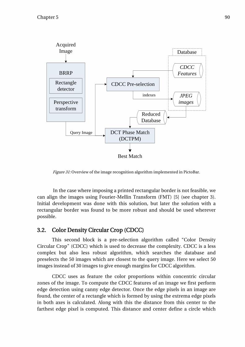
Chapter 5 90

In the case where imposing a printed rectangular border is not feasible, we can align the images using Fourier-Mellin Transform (FMT) [5] (see chapter 3). Initial development was done with this solution, but later the solution with a rectangular border was found to be more robust and should be used wherever possible.

3.2. Color Density Circular Crop (CDCC)

This second block is a pre-selection algorithm called “Color Density Circular Crop” (CDCC) which is used to decrease the complexity. CDCC is a less complex but also less robust algorithm, which searches the database and preselects the 50 images which are closest to the query image. Here we select 50 images instead of 30 images to give enough margins for CDCC algorithm.

CDCC uses as feature the color proportions within concentric circular zones of the image. To compute the CDCC features of an image we first perform edge detection using canny edge detector. Once the edge pixels in an image are found, the center of a rectangle which is formed by using the extrema edge pixels in both axes is calculated. Along with this the distance from this center to the farthest edge pixel is computed. This distance and center define a circle which

Acquired Image

BRRP

CDCC Pre-selection

Reduced Database


JPEG images

Query Image

CDCC Features

Database

indexes

Best Match

Rectangle detector

Perspective transform

Figure 31: Overview of the image recognition algorithm implemented in PictoBar.

Chapter 5 91

tightly encompasses all the edge pixels. This circle is then divided into four concentric regions and the color density of the red, green, and blue channels for each concentric region is calculated. These color densities are assembled in a feature vector of length 𝐿 = 12 which uniquely represents the image (see chapter 3).

For every image stored in the database, the feature vector is pre-calculated and stored. When a query image is presented, the feature vector of the query is calculated and compared with the feature vector of each of the images stored in the database. As the feature vector length is small and also low in complexity to compute, the CDCC algorithm is low in complexity. Additionally, this algorithm is robust to rotation, scaling, and translation, but is sensitive to variations in lighting. This sensitivity to lighting variation can be compensated by using fixed LEDs and calibrating the device using a calibration image (see subsection 3.4).

3.3. DCT Phase Match (DCTPM)

The third block is the base recognition algorithm, which is referred to as “DCT phase match” (DCTPM). This algorithm is accurate and robust to lighting variation but computationally expensive and not RST invariant. To reduce the overall complexity of the system while keeping good accuracy, DCT phase match is only performed on the reduced database of the 50 images pre-selected by the CDCC algorithm.

DCTPM searches for the best match of the query image into the database using correlation on the DCT phase of the 8x8 blocks of the images, and therefore is compatible with the JPEG compression standard (see chapter 3).

The output of BRRP block cannot detect and correct for the image rotation by 180 degrees, as the rectangle is identical if it is rotated by 180 degrees or by 0 degrees. This case is thus tested in the DCTPM block by correlating the DCT phase of the query image with the DCT phase of the 50 images pre-selected by the CDCC algorithm and their 180-degree rotated version.

3.4. Camera setup and calibration

The camera used is a OV7675-MFSL a “flex” module (optics + sensor) from OmniVision. This module contains an OV7675 color camera sensor from OmniVision [58] with fixed focus and VGA resolution (640x480 pixels). Considering the different specifications for PictoBar:

• The distance between the camera and the image (camera height) is fixed such that a VGA resolution acquired image (640 x 480 pixels) corresponds to a rectangle of 8 x 6 cm.

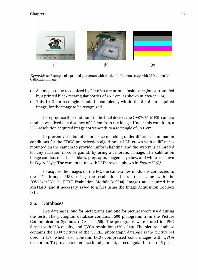
Chapter 5 92

• All images to be recognized by PictoBar are printed inside a region surrounded by a printed black rectangular border of 4 x 3 cm, as shown in Figure 32(a).

• This 4 x 3 cm rectangle should be completely within the 8 x 6 cm acquired image, for the image to be recognized.

To reproduce the conditions in the final device, the OV07675-MFSL camera module was fixed at a distance of 9.2 cm from the image. Under this condition, a VGA resolution acquired image corresponds to a rectangle of 8 x 6 cm.

To prevent variation of color space matching under different illumination conditions for the CDCC pre-selection algorithm, a LED crown with a diffuser is mounted on the camera to provide uniform lighting, and the system is calibrated for any variation in color gamut, by using a calibration image. The calibration image consists of strips of black, grey, cyan, magenta, yellow, and white as shown in Figure 32(c). The camera setup with LED crown is shown in Figure 32(b).

To acquire the images on the PC, the camera flex module is connected to the PC through USB using the evaluation board that came with the “OV7670/OV7171 ECXF Evaluation Module kit”[90]. Images are acquired into MATLAB (and if necessary saved to a file) using the Image Acquisition Toolbox [91].

3.5. Databases

Two databases, one for pictograms and one for pictures were used during the tests. The pictogram database contains 1500 pictograms from the Picture Communication Symbols (PCS) set [56]. The pictograms were stored in JPEG format with 85% quality, and QVGA resolution (320 x 240). The picture database contains the 1000 pictures of the COREL photograph database is the picture set used in [57] which also contains JPEG compressed color images with QVGA resolution. To provide a reference for alignment, a rectangular border of 5 pixels

(a) (b) (c)

Figure 32: (a) Example of a printed pictogram with border (b) Camera setup with LED crown (c) Calibration image.

Chapter 5 93

line-width was added around the images. We refer to these two databases as the “clean pictogram database” and the “clean picture database”.

A subset of 50 representative pictograms and 50 representative pictures was selected from the 1500 pictograms and 1000 pictures of the “clean database” and were printed, along with the added border, on paper with size of 4 x 3 cm as shown in Figure 32(a). The 50 printed pictograms and the 50 printed pictures were then acquired with the camera, from MATLAB. These acquired images constitute respectively the “real condition pictogram database” and the “real condition picture database”.

3.6. MATLAB demonstrator

A demonstrator with a Graphical User Interface (GUI) for PictoBar’s image recognition algorithms was programmed in MATLAB for testing and development. The demonstrator uses as input the image acquired by the camera assembly which is shown in Figure 32(b). The image is acquired from the camera into MATLAB using the image acquisition toolbox. A screenshot of the demonstrator and its explanation is shown in Figure 33.

Before running the PictoBar demonstrator, the image database has to be trained. To train the image database, the CDCC features and the DCT phases from the image database are pre-extracted and stored. The phase of the 180-degree rotated version of the images is also stored, because this situation cannot be detected and corrected in the BRRP block, and it is thus tested in the DCTPM block by correlating the DCT phase of the query image with the DCT phase of the 50 images in the reduced database and its 180-degree rotated version.

It should be noted that for the MATLAB demonstrator, we pre-extract and store the DCT-phase separately for all the images in the database. However for the DSP implementation we calculate the DCP-phase on-the-fly from JPEG compressed images.

Chapter 5 94

4 DSP implementation

After implementing and validating the image recognition algorithm in MATLAB as explained in chapter 3 and chapter 4, the algorithm was ported on the target, which is a DM6446 dual core processor from Texas Instruments [88] containing an ARM9 core and a fixed point C64x+ DSP core. The MATLAB implementation is used as a reference throughout the DSP implementation.

4.1. TMS320DM6446

The TMS320DM6446, also referenced as DM6446, is a dual-core architecture System on Chip (SoC) from Texas Instruments (TI). It has the advantages of both DSP and a Reduced Instruction Set Computer (RISC) technologies, incorporating a high-performance TMS320C64x+™ DSP core and an ARM926EJ-S core [92]. The ARM926EJ-S is a 32-bit RISC processor with pipelining so that all parts of the processor and memory system can operate continuously. The TMS320C64x+™ DSP is a high-performance fixed-point DSP

Figure 33: A screen shot of the demonstrator program is shown. (1) is used to calibrate the device with the calibration image (2) is used to acquire an image from the camera and perform BRRP+CDCC+DCTPM algorithm (3) shows the image acquired from the camera (4) shows the output of the border detection block (5) shows the cropped and preprocessed image which is sent to the CDCC+DCTPM blocks (6) shows the first 12 images of the reduced database output of the CDCC stage (7) shows the best match of the DCTPM stage (8) This field is used to display any error messages encountered.

1

2

3 4 5 7

6

8

Chapter 5 95

based on an enhanced version of the second-generation high-performance, advanced Very Long Instruction Word (VLIW) architecture from Texas Instruments.

The C64x+ core has a performance of up to 6480 Million Instructions Per Second (MIPS) at a clock rate of 810 MHz. The C64x+ DSP core processor has 64 general-purpose registers of 32-bit word length and eight highly independent functional units: two multipliers for a 32-bit result and six Arithmetic Logic Units (ALUs). The eight functional units include instructions to accelerate the performance in video and imaging applications. The DSP core can produce four 16-bit Multiply And Accumulates (MACs) per cycle for a total of 3240 Million MACs per second (MMACS) or eight 8-bit MACs per cycle for a total of 6480 MMACS. The DM6446 device includes a Video Processing Subsystem (VPSS) which can be used as a coprocessor of the C64x+ and has a Video Processing Front-End (VPFE) input used for video capture and a Video Processing Back-End (VPBE) output with imaging co-processor (VICP) used for display.

The DM6446 also offers a rich peripheral set including Asynchronous External Memory Interface (EMIF), Audio Serial Port (ASP), Inter-Integrated Circuit module (I2C), Multimedia Card (MMC) / Secure Digital (SD) card controller, Universal Serial Bus (USB) etc., which provides the ability to control external peripheral devices and to communicate with external processors.

The DM6446 has a complete set of development tools for both the ARM and the DSP. These tools include C compilers and DSP assembly optimizer to simplify programming and scheduling.

4.2. Software framework

A major advantage of programmable signal processors over fixed-function devices is their ability to accelerate multiple multimedia functions and provide flexible environments to enable user customization. However, sharing limited embedded hardware resources between different algorithms, as well as between multiple instances of the same algorithm, can be challenging. Systems can be further complicated when algorithms are independently provided by different vendors.

The Multimedia Framework Products (MFP) [93] is a collection of related software components that are completely open source. MFP includes TI's XDAIS algorithm standard, Framework Components, Linux Utils, WinCE Utils, and Codec Engine. TI's XDAIS algorithm standard provides the rules and guidelines necessary to solve the integration problems mentioned in the previous paragraph. The additional products in the MPF suite build on this standard to provide scalable services that insulate higher-level applications and frameworks from these complexities.

Chapter 5 96

4.2.1. xDAIS and xDM

“eXpressDSP Algorithm Interoperability Standard”, known as XDAIS [94], provides the rules and guidelines necessary to enable integration and execution of algorithms. It provides C/C++ compatible headers for defined interfaces that the algorithms can implement and the applications can invoke. These interfaces enable algorithms to safely share resources, including memory, DMA, and other hardware accelerators. “eXpressDSP Digital Media” (xDM) [95] specifies a standard API (Application Programming Interface) for the application to call a particular algorithm class. The APIs defined in the xDM standard are also referred to as the VISA (video, image, speech and audio) APIs. The use of these APIs facilitates the replacement of an implemented algorithm from a provider by another algorithm from a different provider if a different functionality or performance is required.

4.2.2. HLOS: Linux Utils and WinCE Utils

High Level Operating Systems (HLOS) such as Linux and WinCE don’t allow direct access to hardware resources often needed for efficient implementation of algorithms. Linux Utils [96] and WinCE Utils [97] provide user mode access to these resources. In particular, they provide the ability to allocate physically contiguous memory (CMEM) [98] for the data used by the algorithms. This is a critical feature since accelerators and DSPs generally lack a Memory Management Unit (MMU).

4.2.3. Framework Components

XDAIS provides interfaces for algorithm management and resource sharing. Framework Components (FC) [99] provides low-level libraries that use these XDAIS interfaces for creating, executing, and deleting algorithms (DSKT2), as well as managing algorithm resources (RMAN and DMAN3). This enables users to quickly create a customized, XDAIS-compliant framework.

4.2.4. Codec Engine framework

Codec Engine [100] builds on the products in the MFP suite, and provides a complete out-of-the-box framework that enables users to employ XDAIS algorithms with minimal coding. A unique feature is that the algorithms it manages can be ‘local’ (on the same processor as the application) or ‘remote’ (on a different processor than the application), further insulating the application from the hardware on which it is executing. Codec Engine supports WinCE and Linux, and has been ported to multiple other operating systems.

To implement the PictoBar image recognition algorithm we have used the Codec Engine (CE) framework whose software components are shown in Figure 34 [7]. The ARM9 core uses Embedded Linux from Arago project [101] as Operating System (OS). The DSP core uses DSP/BIOSTM 5.x [102] as real-time

Chapter 5 97

kernel. The communication between the ARM and the DSP cores uses DSP/BIOSTM LINK. The application code runs on the ARM core and handles input/output and application processing. To be used in the CE software framework, algorithms have to be xDAIS/xDM compliant and have to be packed into a Real-Time Software Components (RTSC) package [103]. To process the signals using these algorithms, the application uses the “VISA” (Video, Image, Speech, Audio) Application Programming Interfaces (APIs) which are provided by Codec Engine along with a generic API called IUNIVERSAL. Codec Engine is divided into a CE Remote Server which runs on the DSP and a CE Client which runs on the ARM.

In other to fit the Codec Engine framework, we have thus implemented the three blocks of the PictoBar image recognition algorithm (see section 3), using C language, and ensuring that they are compatible with the xDAIS/xDM [95] standards from Texas Instruments. The ARM application, written in C language, manages resources (e.g. memory) as well as the remote execution of the algorithms using the consistent set of Application Programming Interfaces (APIs) called the “VISA” APIs. VISA stands for Video, Imaging, Speech and Audio. Each of these four groups supports encoders and decoders, totaling to eight VISA classes. Additionally, the IUNIVERSAL class is used to manage generic algorithms. For the implementation of the image recognition algorithm of PictoBar, explained in section 4.6, we have used only two classes: IUNIVERSAL (to implement the BRRP, CDCC and DCTPM blocks) and IMGDEC1 (to implement the JPEG decoder). For each of these two classes, the following APIs are provided:

• UNIVERSAL_create(), IMGDEC1_create() - Creates an instance of the algorithm, and allocates the required resources for the algorithm to run.

• UNIVERSAL_process(), IMGDEC1_ process() - Execute the "process" method in the specified instance of the algorithm. Block until complete.

• UNIVERSAL_control(), IMGDEC1_control() - Execute the "control" method in the specified instance of the algorithm, to modify parameters that control the algorithm.

• UNIVERSAL_delete(), IMGDEC1_delete() - Delete the specified instance of the algorithm and reclaims the resources allocated with create().

More information on the xDAIS/xDM interfaces is found in the “xDAIS Interface Reference” [104].

4.3. Development environment

For the development of the DSP implementation on DM6446 we have used the EVMDM6446 from Spectrum Digital [105] as development board. The

Chapter 5 98

development board runs Arago Linux on the ARM core and DSP/BIOS v5 on the DSP core.

For the software development a virtual machine running Ubuntu 10.04 was used. The required software components for development like the GNU toolchain, software development kit (DVSDK) and tools, Processor Support Package (PSP) were installed on this Ubuntu virtual machine. Code composer studio (CCS) v4 was also installed on the virtual machine and along with a Blackhawk USB-JTAG emulator (BH-USB-560BP) [106] was used to debug the algorithms.

The file system of the EVMDM6446 development board is put on a network server with a fixed IP address and mounted using Network File System (NFS). The board, configured to boot from Flash NAND, is connected to the network and is assigned a fixed IP address. This setup allows the access from remote locations to the file system via Samba or NFS and facilitates remote login and execution on the board using SSH or Telnet.

4.4. ARM application

The device application runs on the ARM core which uses “Arago” [101] embedded linux kernel and file system. The application features user interface, barcode recognition algorithm, file I/O and database management, communication with the PC, overall system management and control of peripherals such as audio I/O and camera image acquisition. Additionally, the

Figure 34: Codec Engine (CE) framework components.

Chapter 5 99

ARM application controls the remote execution of the image recognition algorithm on the C64x+ DSP core using Codec Engine framework.

The ARM application manages, using VISA commands, the remote execution on C64+ of the algorithm blocks (BRRP, CDCC, DCTPM, JPEGDEC) which are implemented as four separate “codecs” (algorithm packages) as explained in subsection 4.6.

The ARM application is used to initialize, load, execute, and delete all the algorithms and the DSP Engine. At the beginning of its execution, the ARM application initializes all the required buffers and other parameters for the different algorithms in subsection 4.6. It then resets, loads, and starts the DSP engine. It allocates and initializes the BRRP algorithm in the DSP engine and gets an image file, in YUV 4:2:2 format, as the input (see chapter 3 subsection 1.1.2), reads the image file and executes the BRRP algorithm on this image to detect the printed border, align, crop, and pre-process the image, to produce the query image for the CDCC and DCTPM stages. After successful execution the BRRP algorithm is deleted in the DSP engine. The corrected query image from the BRRP algorithm is passed to the CDCC input buffers.

The CDCC algorithm is initialized in the DSP engine and the application uses the CDCC algorithm to extract the CDCC features from the corrected query image. Later it calls the CDCC algorithm to perform distance calculation between the features of the query image and the features of the images in the database stored in a pre-extracted file, followed by sorting the calculated distances and selecting the top 50 images, which have the shortest distance to the query image, to be used as reduced database for the DCTPM stage. After successful execution the CDCC algorithm is deleted in the DSP engine and the list of top 50 images is passed to the input buffers of the DCTPM algorithm.

Then the DCTPM and JPEGDEC algorithms are initialized in the DSP engine and the application first calls the DCTPM algorithm to calculate the DCT phase of the query image. Then, for each of the candidate images from the list passed by CDCC algorithm along with their 180 degree rotated versions, it reads the candidate image from file; it calls the JPEGDEC algorithm to decompress the image to YUV422 format; it calls the DCTPM algorithm to extract the luminance Y and calculate the phase, correlating it with the phase of the query. Finally, it calls the DCTPM algorithm for sorting the 100 calculated correlations and storing the sorted 50 best matched image list as an output file. After performing these operations the DCTPM and JPEGDEC algorithms are deleted to free the memory.

4.5. Libraries

To implement the BRRP, CDCC, and DCTPM blocks, we have used as much as possible the functions from the Image and video processing Library (IMGLIB2)

Chapter 5 100

[107] and the Video Analytics & Vision Library (VLIB) [108] provided by Texas Instruments. To be used in the CE software framework, the IMGLIB2 and VLIB were put in an RTSC package.

IMGLIB2 is a collection of more than 70 building block kernels that can be used for image and video processing applications. The rich set of software routines included in IMGLIB2 perform image processing functionality that includes forward and inverse DCT, quantization, edge detection, image histogram, image thresholding, median filtering, etc.

VLIB is a software library of more than 40 royalty-free kernels from Texas Instruments which accelerates video analytics development and increases performance up to 10 times. VLIB is an extensible library that is optimized for the C6x DSP core and is available royalty-free. This collection of 40+ kernels provides the ability to perform low-level pixel processing, object feature extraction, and tracking and recognition.

4.6. CODECS

In order to be used under the Codec Engine framework, an algorithm must be implemented as an xDAIS/xDM-compliant package also referred to as a “codec”. The algorithm blocks implemented in the Codec Engine framework are BRRP, CDCC, DCTPM and JPEG decoder. Each of these blocks was implemented as a separate Codec Engine “codec”. The BRRP, CDCC and DCTPM codecs were implemented using the IUNIVERSAL xDM standard interface [103]. We have used the Codec Engine GenCodecPkg wizard [109] to generate each codec package containing starter code and then we have added the C code of the algorithm blocks into it, using fixed point arithmetic and calls to functions from the Image and Vision libraries from Texas Instruments, IMGLIB2 and VLIB (see subsection 4.5).

4.6.1. BRRP

The BRRP codec initially converts the acquired UYVY image into a planar RGB image using functions from the VLIB library. The RGB image is converted into a grey image which is then used to extract the corners of the rectangular border by using Harris corner detector, verifying the extracted corners using SUSAN. These corners of the rectangular border are used to compensate for any geometrical transformations using perspective transform. Then, histogram stretching is performed using the parameters in a file named ‘calibration_parameters.c’. The parameters in this file were written during the process of calibration using the calibration image (see subsection 3.4).

Chapter 5 101

4.6.2. CDCC

The CDCC algorithm block was implemented using the IUNIVERSAL xDM interface. It uses functions from the IMGLIB2 and VLIB library to perform Canny edge detection and Gaussian filtering of the images. The implemented algorithm modes used by the ARM application to call the corresponding operations in the CDCC codec are:

• ‘ICDCC_MODE_CALC_FEATURE’ – This mode is used to calculate the CDCC features. Initially the RGB image is converted into a greyscale image. Then, frame based Canny edge detection is applied on this greyscale image. The centroid of the edge image and the radius are computed. The CDCC feature for each image plane (red, green, and blue) is computed and stored.

• ‘ICDCC_MODE_CALC_DISTANCE’ – This mode is used to calculate the CDCC feature distances between the query image and the images in the database. The pre-extracted CDCC features which are used in this mode are stored in the file ‘image_database.c’.

• ‘ICDCC_MODE_SORT_DISTANCE’ – This mode is used to sort the calculated CDCC feature distances and rank the images.

4.6.3. DCTPM

The three algorithm modes used by the ARM application to call the corresponding operations in the DCTPM codec are:

• ‘IDCTPM_MODE_CALC_QPHA’ – This mode is used to calculate the DCT phase of the query image. The luminance Y of the query is extracted. The 320 x 240 pixels of the luminance Y is considered as an array of 30 x 40 8x8-block elements. For each of the 40 columns, its 30 8x8 blocks are first copied from slow external memory to fast internal memory. Then, for each of these blocks, we calculate the DCT followed by quantization and extraction of the phase from quantized DCT values.

• ‘IDCTPM_MODE_CALC_CORR’ – This mode is used to calculate the DCT phase of a candidate image (which was JPEG decompressed to YUV422) and correlate it with the DCT phase of the query. The luminance Y of the candidate image is extracted. The 320 x 240 pixels of the luminance Y is considered as an array of 30x40 8x8-block elements. For each of the 40 columns, its 30 8x8 blocks are first copied from slow external memory to fast internal memory. We then calculate the DCT for each of these blocks, followed by quantization and extraction of the phase from the quantized DCT values. After the phase of the candidate image is extracted, it is correlated with the phase of the query image, and the resulting correlation is stored.

• ‘IDCTPM_MODE_SORT_CORR’- This mode is used to sort the calculated correlations to find the best match.

Chapter 5 102

4.6.4. JPEG decoder

We have used the JPEG Decoder for C64x+ Version 02.00.02 provided by Texas Instruments [110], which is delivered as a Real-Time Software Components (RTSC) package containing a IIMGDEC1 xDM codec [103]. The JPEG decoder is used to decompress the candidate images for the DCTPM.

4.7. Testing

The board setup (see subsection 4.3) allows access from remote location to the file system via Samba or NFS and facilitates remote login and execution on the board using Telnet or SSH. This allows sharing of the development board between users and the possibility to perform extensive testing automatically from MATLAB: first the input files are written from MATLAB on the board file system, execution of the application on the board is controlled from MATLAB using SSH, and the output files are read by MATLAB from the board file system to analyze the results. Using this development setup, we have extensively tested the CDCC and DCTPM blocks; with images from the “clean database” (see subsection 3.5). By comparing the results from the DSP implementation with the results from the MATLAB implementation, we have verified the proper functioning of the DSP implementation, and that the losses due to the fixed-point arithmetic of the C64x+ do not affect the performance. Code Composer Studio (CCS v4) [111] from Texas Instruments along with a Blackhawk USB-JTAG emulator (BH-USB-560BP) [106] were also used as debugging tool to verify DSP implementation.

4.8. Results

After validating each block (codec) individually, the DSP implementation of the concatenated BRRP, CDCC and DCTPM blocks was also tested using the test setup described in subsection 4.7 , using the union of the two clean databases for pictures and pictogram with border, containing 2500 images. Every image from this database is successively used as query, running the search for this image on the entire database. Tests were also performed with different rotations of the query image at 30, 60 and 90 degrees. The recognition accuracy is calculated as the proportion of cases in which the best match corresponds to the query image, with respect to the number of trials. We also performed tests with the real condition databases. The results of these tests are shown in Table 8. We can see that the DSP implemented image recognition system performs very well with both clean databases and real databases. The average recognition time of the DSP implementation of the image recognition system was 0.79 seconds, and the worst case was 0.93 seconds, which is within the target specification for the device (see section 2.2).

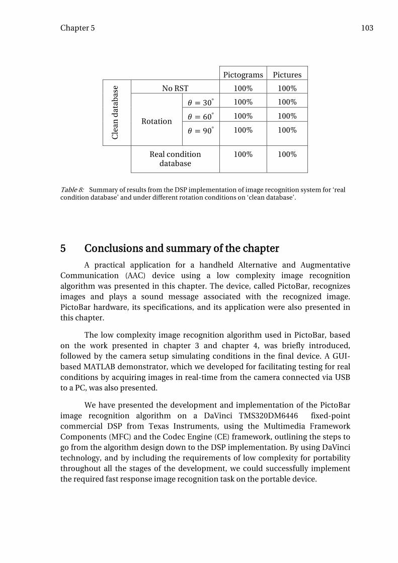
Chapter 5 103


A practical application for a handheld Alternative and Augmentative Communication (AAC) device using a low complexity image recognition algorithm was presented in this chapter. The device, called PictoBar, recognizes images and plays a sound message associated with the recognized image. PictoBar hardware, its specifications, and its application were also presented in this chapter.

The low complexity image recognition algorithm used in PictoBar, based on the work presented in chapter 3 and chapter 4, was briefly introduced, followed by the camera setup simulating conditions in the final device. A GUI-based MATLAB demonstrator, which we developed for facilitating testing for real conditions by acquiring images in real-time from the camera connected via USB to a PC, was also presented.

We have presented the development and implementation of the PictoBar image recognition algorithm on a DaVinci TMS320DM6446 fixed-point commercial DSP from Texas Instruments, using the Multimedia Framework Components (MFC) and the Codec Engine (CE) framework, outlining the steps to go from the algorithm design down to the DSP implementation. By using DaVinci technology, and by including the requirements of low complexity for portability throughout all the stages of the development, we could successfully implement the required fast response image recognition task on the portable device.

Pictograms Pictures

Cle

an d

atab

ase No RST 100% 100%

Rotation

𝜃 = 30° 100% 100%

𝜃 = 60° 100% 100%

𝜃 = 90° 100% 100%

Real condition database

100% 100%

Table 8: Summary of results from the DSP implementation of image recognition system for ‘real condition database’ and under different rotation conditions on ‘clean database’.

Chapter 5 104

The image recognition algorithm implemented on the DSP was extensively tested by using a testing scheme which facilitated remote access and control of the DSP from MATLAB. The recognition system implemented on the DSP showed an accuracy of 100% when tested with a database of 2500 images under different test conditions. The average recognition time of the DSP implementation of the image recognition system was 0.79 seconds, and the worst case was 0.93 seconds, which is within the target specification of one second for the device.

Chapter 6

Conclusion

In this chapter we look at the summary and contributions of the PhD work in section 1. We discuss future work and direction of research in section 2.

Chapter 6 106

1 Summary and recall of the contributions

This PhD work contributes to the research in the area of content based image retrieval which uses visual contents or information extracted from the image, to describe the image and to search for its closest match within a database of possible images. In particular, this thesis is focused on algorithms for retrieval of images for portable handheld devices. The work carried out during this PhD includes first an algorithmic development part and then implementation of the developed algorithm on a commercial digital signal processor from Texas Instruments (TMS320DM6446). Two distinct datasets were used to test the algorithms developed during the PhD work and their implementation, namely, a dataset of natural images also referred to as ‘pictures’ (images which have a rich local covariance structure), and a dataset of pictograms (images which have limited color content and variations, and convey a meaning through pictorial representation of a physical object or an action). All the algorithms developed as part of this PhD work are of low complexity, and optimized for DSP implementation in handheld devices.

The PhD work resulted in three main contributions which were presented in chapter 3, chapter 4 and chapter 5 of this document. The first contribution consists of two novel algorithms, ‘Color Density Circular Crop’ (CDCC) and ‘DCT-Phase Match’ (DCTPM), which were introduced to perform image retrieval. The CDCC algorithm is rotation, scaling, and translation invariant, low complexity but less robust. DCTPM algorithm is already designed to achieve certain efficiency (if the image is JPEG encoded it avoids recalculation of the phase, and by using only the ternary phase, it could be efficient for certain architectures). However, although more robust, the DCTPM algorithm is RST variant and still too complex for handheld applications. One significant contribution is the combining of both algorithm into a two-stage algorithm to have low-complexity and good performance at the same time. The proposed two-stage algorithm outperformed the state of the art CBIR algorithms using SIFT, GIST, and color histogram descriptors in terms of execution speed by a factor of 21.33. Moreover, the proposed algorithm had higher accuracy for a specific case of pictograms compared to algorithm using SIFT descriptors.

The second contribution consists of three different rotation, scaling, and translation compensation algorithms that can be used for low-complexity content based image retrieval. This includes two rectangle detection algorithms using either ‘line detection’ or ‘corner detection’ along with geometric deformation correction using ‘perspective transform’, and one compensation algorithm without using any additional printed reference pattern on the image that uses Fourier-Mellin Transform. When used in conjunction with the developed two-stage recognition algorithm, the proposed compensation algorithms showed an average accuracy of 94.05% for FMT-based compensation and 99% and 100% for

Chapter 6 107

line detection- and corner detection- based compensation algorithms respectively.

The third contribution was the development and implementation of the image recognition algorithm on TMS320DM6446 using the Multimedia Framework Components (MFC) and the Codec Engine (CE) framework. An outline of the steps to go from the algorithm design down to the DSP implementation was also presented. A practical application which uses the low complexity image retrieval algorithms developed during this PhD work for a handheld alternative and augmentative communication device called ‘PictoBar’ was also presented. This ‘PictoBar’ device is intended to be used by language re-education professionals and specialized educators in the treatment of people affected by pathologies such as aphasia, autism, trisomy, or mental handicaps.

2 Discussions and future work

The CDCC algorithm developed during the PhD work is fast and robust to rotation, scaling, and translation. However, the algorithm is sensitive to lighting variations. The future work includes exploring ways to make CDCC algorithm insensitive to lighting variation, by using color spaces with no intensity information. This would improve robustness and avoid frequent calibration of the device. At the moment, we use LEDs to provide uniform lighting and carefully calibrate the system against variations in lighting by using a calibration image. Furthermore automatic calibration for every image can be made by printing a calibration pattern along the border and using this pattern every time when an image is captured by the camera to calibrate the device.

The DCTPM algorithm is partially robust to lighting variation and is sensitive to geometrical transformations like rotation, scaling, and translation.

(a) (b) (c)

Figure 35: (a) First prototype of PictoBar device, (b) Design of the final PictoBar device, (c) Current prototype of the PictoBar device.

Chapter 6 108

Hence to compensate for these geometrical transformations, we use the developed compensation algorithms presented in chapter 4. Future work would involve development of invariant phase features to be used for image recognition which could be based, e.g, on Fourier-Mellin transform. This would eliminate the need for any additional rotation, scaling, and translation compensation algorithms.

The algorithms and methods presented in this PhD work were successfully incorporated into the ‘PictoBar’ device. The developed algorithms and its implementation satisfied the target specifications of ‘PictoBar’ device. The image recognition algorithm implemented on the DSP showed an accuracy of 100% under different test conditions for a representative set of 2500 pictures and pictograms. The average recognition time of the DSP implementation of the image recognition system was 0.79 seconds which is below the required specification of one second.

The ‘PictoBar’ device is currently in the pre-industrialization phase where the image recognition algorithms are being integrated with the device control and overall system management of the device. A picture of the first prototype along with the current prototype is shown in Figure 35. Future work includes development of an advanced rejection strategy that should be implemented in PictoBar before training a new image to be put into the database of the device. This rejection strategy would be based on a DCTPM search which should be done with the new image as query on the database already trained into the device. If the new image is too similar to one or more images in the database, it should be rejected and the user warned that the images are too close. The preliminary tests have shown that it would be suitable to select the threshold for rejection based on the DCT phase correlation of the second and further best matches, normalized by the correlation of the best match in the DCTPM search.

The DSP implementation is currently within the response time specifications of PictoBar. Proper file arrangement of the image database and buffering into memory should be considered at the level of the application software for further lowering the response time. Further optimization at the DSP level could be done by using the HW accelerators of the TMS320DM6446, such as the VCIP and the resizer, by improved cache management or by further algorithm and/or code optimizations.

References

[1] J. Clottes, P. G. Bahn, and M. Arnold, Chauvet Cave: The Art of Earliest Times: University of Utah Press, 2003.

[2] H. Gernsheim, A Concise History of Photography: Third Revised Edition: Dover, 1986.

[3] P. Ayyalasomayajula, S. Grassi, and P. A. Farine, "Rotation, scale and translation invariant image retrieval method based on circular segmentation and color density," in Image and Signal Processing and Analysis (ISPA), 2011 7th International Symposium on, 2011, pp. 455-459.

[4] P. Ayyalasomayajula, S. Grassi, and P. A. Farine, "Retrieval of occluded images using DCT phase and region merging," in Image Processing, 2012. ICIP 2012. IEEE International Conference on, 2012.

[5] P. Ayyalasomayajula, S. Grassi, and P. A. Farine, "Low complexity RST invariant image recognition using Fourier Mellin transform," in European Signal Processing Conference. EUSIPCO 2011 Barcelona, Spain, 2011, pp. 769 - 773.

[6] P. Ayyalasomayajula, S. Grassi, and P. A. Farine, "Low complexity image recognition algorithm for handheld applications," in Ph.D. Research in Microelectronics and Electronics (PRIME), 2011 7th Conference on, 2011, pp. 165-168.

[7] P. Ayyalasomayajula, S. Grassi, N. Deurin, P. Farine, and T. Gueguen, "Implementation of an image recognition algorithm on the DM6446 DaVinci processor," in Education and Research Conference (EDERC), 2010 4th European, 2010, pp. 175-179.

[8] T. Kato, T. Kurita, N. Otsu, and K. Hirata, "A sketch retrieval method for full color image database-query by visual example," in Pattern Recognition, 1992. Vol.I. Conference A: Computer Vision and Applications, Proceedings., 11th IAPR International Conference on, 1992, pp. 530-533.

[9] J. Eakins and M. Graham, "Content-based image retrieval," ed: JTAP, 1999.

References 110

[10] E. Hyvönen, S. Saarela, A. Styrman, and K. Viljanen, "Ontology-Based Image Retrieval," in WWW (Posters), 2003.

[11] C. Carson, S. Belongie, H. Greenspan, and J. Malik, "Blobworld: image segmentation using expectation-maximization and its application to image querying," Pattern Analysis and Machine Intelligence, IEEE Transactions on, vol. 24, pp. 1026-1038, 2002.

[12] G. Borba, H. Gamba, L. Mayron, and O. Marques, "Integrated global and object-based image retrieval using a multiple examples query schema," in International Conference on Computer Vision Theory and Applications (VISAPP), 2007.

[13] S. Santini and R. Jain, "The Graphical Specification of Similarity Queries," Journal of Visual Languages & Computing, vol. 7, pp. 403-421, 1996.

[14] Y. Wang, T. Mei, J. Wang, H. Li, and S. Li, "JIGSAW: interactive mobile visual search with multimodal queries," presented at the Proceedings of the 19th ACM international conference on Multimedia, Scottsdale, Arizona, USA, 2011.

[15] R. Datta, D. Joshi, J. Li, and J. Wang, "Image retrieval: Ideas, influences, and trends of the new age," ACM Comput. Surv., vol. 40, pp. 1-60, 2008.

[16] S. Santini and R. Jain, "Similarity measures," Pattern Analysis and Machine Intelligence, IEEE Transactions on, vol. 21, pp. 871-883, 1999.

[17] B. Moghaddam, C. Nastar, and A. Pentland, "A Bayesian similarity measure for direct image matching," in Pattern Recognition, 1996., Proceedings of the 13th International Conference on, 1996, pp. 350-358.

[18] S.-H. Cha, "Comprehensive survey on distance/similarity measures between probability density functions," International Journal of Mathematical Models and Methods in Applied Sciences, vol. 1, pp. 300-307, 2007.

[19] A. Joly, O. Buisson, and C. Frelicot, "Content-based copy retrieval using distortion-based probabilistic similarity search," Multimedia, IEEE Transactions on, vol. 9, pp. 293-306, 2007.

[20] M. Swain and D. Ballard, "Color indexing," International Journal of Computer Vision, vol. 7, pp. 11-32, 1991/11/01 1991.

[21] G. H. Joblove and D. Greenberg, "Color spaces for computer graphics," SIGGRAPH Comput. Graph., vol. 12, pp. 20-25, 1978.

[22] G. Pass and R. Zabih, "Histogram refinement for content-based image retrieval," in Applications of Computer Vision, 1996. WACV '96., Proceedings 3rd IEEE Workshop on, 1996, pp. 96-102.

[23] C. Carson, M. Thomas, S. Belongie, J. Hellerstein, and J. Malik, "Blobworld: a System for Region-based Image Indexing and Retrieval," University of California at Berkeley 1999.

[24] O. Pele and M. Werman, "The quadratic-chi histogram distance family," presented at the Proceedings of the 11th European conference on Computer vision: Part II, Heraklion, Crete, Greece, 2010.

[25] G. W. Snedecor and W. G. Cochran, "Statistical methods," 1967.

[26] J. Hafner, H. S. Sawhney, W. Equitz, M. Flickner, and W. Niblack, "Efficient color histogram indexing for quadratic form distance functions," Pattern Analysis and Machine Intelligence, IEEE Transactions on, vol. 17, pp. 729-736, 1995.

References 111

[27] Y. Rubner, C. Tomasi, and L. J. Guibas, "The earth mover's distance as a metric for image retrieval," International Journal of Computer Vision, vol. 40, pp. 99-121, 2000.

[28] M. Stricker and M. Orengo, "Similarity of color images," in Proc. SPIE Storage and Retrieval for Image and Video Databases, 1995, p. 4.

[29] F. Mindru, T. Tuytelaars, L. V. Gool, and T. Moons, "Moment invariants for recognition under changing viewpoint and illumination," Computer Vision and Image Understanding, vol. 94, pp. 3-27, 4// 2004.

[30] K. E. A. van de Sande, T. Gevers, and C. G. M. Snoek, "Evaluating Color Descriptors for Object and Scene Recognition," Pattern Analysis and Machine Intelligence, IEEE Transactions on, vol. 32, pp. 1582-1596, 2010.

[31] D. G. Lowe, "Object recognition from local scale-invariant features," in Computer Vision, 1999. The Proceedings of the Seventh IEEE International Conference on, 1999, pp. 1150-1157 vol.2.

[32] J. S. Beis and D. G. Lowe, "Shape indexing using approximate nearest-neighbour search in high-dimensional spaces," in Computer Vision and Pattern Recognition, 1997. Proceedings., 1997 IEEE Computer Society Conference on, 1997, pp. 1000-1006.

[33] N. Dalal and B. Triggs, "Histograms of oriented gradients for human detection," in Computer Vision and Pattern Recognition, 2005. CVPR 2005. IEEE Computer Society Conference on, 2005, pp. 886-893 vol. 1.

[34] F. Suard, A. Rakotomamonjy, A. Bensrhair, and A. Broggi, "Pedestrian Detection using Infrared images and Histograms of Oriented Gradients," in Intelligent Vehicles Symposium, 2006 IEEE, 2006, pp. 206-212.

[35] A. Oliva and A. Torralba, "Modeling the Shape of the Scene: A Holistic Representation of the Spatial Envelope," Int. J. Comput. Vision, vol. 42, pp. 145-175, 2001.

[36] J. Sivic and A. Zisserman, "Video Google: A text retrieval approach to object matching in videos," in Computer Vision, 2003. Proceedings. Ninth IEEE International Conference on, 2003, pp. 1470-1477.

[37] L. Fei-Fei and P. Perona, "A Bayesian hierarchical model for learning natural scene categories," in Computer Vision and Pattern Recognition, 2005. CVPR 2005. IEEE Computer Society Conference on, 2005, pp. 524-531 vol. 2.

[38] D. G. Lowe, "Distinctive Image Features from Scale-Invariant Keypoints," Int. J. Comput. Vision, vol. 60, pp. 91-110, 2004.

[39] K. Mikolajczyk and C. Schmid, "Scale & affine invariant interest point detectors," International journal of computer vision, vol. 60, pp. 63-86, 2004.

[40] S. Savarese, J. Winn, and A. Criminisi, "Discriminative object class models of appearance and shape by correlatons," in Computer Vision and Pattern Recognition, 2006 IEEE Computer Society Conference on, 2006, pp. 2033-2040.

[41] E. B. Sudderth, A. Torralba, W. T. Freeman, and A. S. Willsky, "Learning hierarchical models of scenes, objects, and parts," in Computer Vision, 2005. ICCV 2005. Tenth IEEE International Conference on, 2005, pp. 1331-1338.

[42] J. C. Niebles and L. Fei-Fei, "A hierarchical model of shape and appearance for human action classification," in Computer Vision and Pattern Recognition, 2007. CVPR'07. IEEE Conference on, 2007, pp. 1-8.

References 112

[43] S. Belongie, J. Malik, and J. Puzicha, "Shape matching and object recognition using shape contexts," Pattern Analysis and Machine Intelligence, IEEE Transactions on, vol. 24, pp. 509-522, 2002.

[44] M. Unser, "Splines: a perfect fit for signal and image processing," Signal Processing Magazine, IEEE, vol. 16, pp. 22-38, 1999.

[45] H. Bay, T. Tuytelaars, and L. Van Gool, "Surf: Speeded up robust features," Computer Vision–ECCV 2006, pp. 404-417, 2006.

[46] J. Malik, S. Belongie, J. Shi, and T. Leung, "Textons, contours and regions: Cue integration in image segmentation," in Computer Vision, 1999. The Proceedings of the Seventh IEEE International Conference on, 1999, pp. 918-925.

[47]

[48] B. Gadat and L. Younes, "A Stochastic Algorithm for Feature Selection in Pattern Recognition," J. Mach. Learn. Res., vol. 8, pp. 509-547, 2007.

[49] Y. Liu, D. Zhang, G. Lu, and W.-Y. Ma, "A survey of content-based image retrieval with high-level semantics," Pattern Recognition, vol. 40, pp. 262-282, 2007.

[50] A. Krizhevsky, I. Sutskever, and G. Hinton, "Imagenet classification with deep convolutional neural networks," in Advances in Neural Information Processing Systems 25, 2012, pp. 1106-1114.

[51] I. Newton, Opticks: Dover Publications, 1952.

[52] S. Beeson and J. W. Mayer, Patterns of Light: Chasing the Spectrum from Aristotle to LEDs: Springer, 2008.

[53] J. T. McIlwain, An Introduction to the Biology of Vision: Cambridge University Press, 1996.

[54] T. Young, "The Bakerian Lecture: On the Theory of Light and Colours," Philosophical Transactions of the Royal Society of London, vol. 92, pp. 12-48, January 1, 1802.

[55] J. Canny, "A Computational Approach to Edge Detection," Pattern Analysis and Machine Intelligence, IEEE Transactions on, vol. PAMI-8, pp. 679-698, 1986.

[56] http://www.mayer-johnson.com/pcs-collections/. (2008). Picture Communication Symbols.

[57] J. Z. Wang, L. Jia, and G. Wiederhold, "SIMPLIcity: semantics-sensitive integrated matching for picture libraries," Pattern Analysis and Machine Intelligence, IEEE Transactions on, vol. 23, pp. 947-963, 2001.

[58] OmniVision. OV7675 CMOS VGA (640 x 480) Image Sensor with OmniPixel3-HS Technology. Available: http://www.ovt.com/products/sensor.php?id=75

[59] M. Shneier and M. Abdel-Mottaleb, "Exploiting the JPEG compression scheme for image retrieval," Pattern Analysis and Machine Intelligence, IEEE Transactions on, vol. 18, pp. 849-853, 1996.

[60] N. Ahmed, T. Natarajan, and K. R. Rao, "Discrete Cosine Transform," Computers, IEEE Transactions on, vol. C-23, pp. 90-93, 1974.

[61] I. Ito and H. Kiya, "DCT Sign-Only Correlation with Application to Image Matching and the Relationship with Phase-Only Correlation," in Acoustics, Speech and Signal Processing, 2007. ICASSP 2007. IEEE International Conference on, 2007, pp. I-1237-I-1240.

http://www.mayer-johnson.com/pcs-collections/

http://www.ovt.com/products/sensor.php?id=75

References 113

[62] J. Bracamonte, M. Ansorge, F. Pellandini, P.-A. Farine, W.-K. Leow, M. Lew, T.-S. Chua, W.-Y. Ma, L. Chaisorn, and E. Bakker, "Efficient Compressed Domain Target Image Search and Retrieval." vol. 3568, ed: Springer Berlin / Heidelberg, 2005, pp. 594-594.

[63] K. Miyazawa, K. Ito, T. Aoki, K. Kobayashi, and H. Nakajima, "An efficient iris recognition algorithm using phase-based image matching," in Image Processing, 2005. ICIP 2005. IEEE International Conference on, 2005, pp. II-49-52.

[64] F. Arnia, I. Iizuka, M. Fujiyoshi, and H. Kiya, "Fast Method for Joint Retrieval and Identification of JPEG Coded Images Based on DCT Sign," in Image Processing, 2007. ICIP 2007. IEEE International Conference on, 2007, pp. II - 229-II - 232.

[65] I. Ito and H. Kiya, "A new class of image registration for guaranteeing secure data management," in Image Processing, 2008. ICIP 2008. 15th IEEE International Conference on, 2008, pp. 269-272.

[66] W. B. Pennebaker and J. L. Mitchell, JPEG Still Image Data Compression Standard: Kluwer Academic Publishers, 1992.

[67] M. Sonka, V. Hlavac, and R. Boyle, Image processing, analysis, and machine vision: Thompson Learning, 2008.

[68] L. J. Chipman, T. M. Orr, and L. N. Graham, "Wavelets and image fusion," in Image Processing, 1995. Proceedings., International Conference on, 1995, pp. 248-251 vol.3.

[69] K. R. Rao and P. Yip, Discrete cosine transform: algorithms, advantages, applications: Academic Press Professional, Inc., 1990.

[70] A. Vedaldi and B. Fulkerson, "{VLFeat}: An Open and Portable Library of Computer Vision Algorithms," ed, 2008.

[71] D. Casasent and D. Psaltis, "Scale invariant optical transform," Optical Engineering, vol. 15, pp. 153258-153258-, 1976.

[72] T. Yatagai, K. Choji, and H. Saito, "Pattern classification using optical Mellin transform and circular photodiode array," Optics Communications, vol. 38, pp. 162-165, 1981.

[73] Y. Sheng and H. H. Arsenault, "Experiments on pattern recognition using invariant Fourier-Mellin descriptors," JOSA A, vol. 3, pp. 771-776, 1986.

[74] A. Grace and M. Spann, "A comparison between Fourier-Mellin descriptors and moment based features for invariant object recognition using neural networks," Pattern Recognition Letters, vol. 12, pp. 635-643, 1991.

[75] Q.-s. Chen, M. Defrise, and F. Deconinck, "Symmetric phase-only matched filtering of Fourier-Mellin transforms for image registration and recognition," Pattern Analysis and Machine Intelligence, IEEE Transactions on, vol. 16, pp. 1156-1168, 1994.

[76] M. Gueham, A. Bouridane, D. Crookes, and O. Nibouche, "Automatic recognition of shoeprints using Fourier-Mellin transform," in Adaptive Hardware and Systems, 2008. AHS'08. NASA/ESA Conference on, 2008, pp. 487-491.

[77] X. Wang, B. Xiao, J.-F. Ma, and X.-L. Bi, "Scaling and rotation invariant analysis approach to object recognition based on Radon and Fourier–Mellin transforms," Pattern Recognition, vol. 40, pp. 3503-3508, 2007.

References 114

[78] B. S. Reddy and B. N. Chatterji, "An FFT-based technique for translation, rotation, and scale-invariant image registration," Image Processing, IEEE Transactions on, vol. 5, pp. 1266-1271, 1996.

[79] V. Venkateswar and R. Chellappa, "Extraction of straight lines in aerial images," Pattern Analysis and Machine Intelligence, IEEE Transactions on, vol. 14, pp. 1111-1114, 1992.

[80] G. Roth and M. D. Levine, "Extracting geometric primitives," CVGIP: Image Understanding, vol. 58, pp. 1-22, 1993.

[81] P. V. Hough, "Method and means for recognizing complex patterns," ed: Google Patents, 1962.

[82] P. E. Hart, "How the Hough transform was invented [DSP History]," Signal Processing Magazine, IEEE, vol. 26, pp. 18-22, 2009.

[83] C. Harris and M. Stephens, "A combined corner and edge detector," in Alvey vision conference, 1988, p. 50.

[84] S. M. Smith and J. M. Brady, "SUSAN—A new approach to low level image processing," International journal of computer vision, vol. 23, pp. 45-78, 1997.

[85] I. T. Jolliffe, Principal component analysis vol. 487: Springer-Verlag New York, 1986.

[86] A. Criminisi, I. Reid, and A. Zisserman, "A plane measuring device," Image and Vision Computing, vol. 17, pp. 625-634, 1999.

[87] "PictoBar: Portable augmentative and alternative communication device with pictogram recognition functionality for the speech handicapped.," ed: 8811.2;5 PFNM-NM, Commission for Technology and Innovation 2007.

[88] Texas Instruments Digital Media System-on-Chip TMS320DM6446 Available: http://focus.ti.com/docs/prod/folders/print/tms320dm6446.html

[89] Texas Instruments Low-Power Mono ADC / Stereo DAC with HP/Speaker Amplifier and 12-bit measurement ADC TLV320AIC26. Available: http://focus.ti.com/docs/prod/folders/print/tlv320aic26.html

[90] OmniVision, "OV7670/OV7171 ECXF Evaluation Module Quick Start Guide ", ed, 2008.

[91] MathWorks. Image Acquisition Toolbox. Available: http://www.mathworks.ch/products/imaq/

[92] ARM. ARM926 Processor. Available: http://www.arm.com/products/processors/classic/arm9/arm926.php

[93] Texas Instruments Multimedia Framework Products (MFP) - Codec Engine, Framework Components and XDAIS. Available: http://processors.wiki.ti.com/index.php/Category:MFP

[94] Texas Instruments eXpress DSP Algorithm Interoperability Standard. Available: http://processors.wiki.ti.com/index.php/Category:XDAIS

[95] Texas Instuments (2007). xDAIS-DM (Digital Media) User Guide. Available: http://www.ti.com/lit/ug/spruec8b/spruec8b.pdf

[96] Texas Instruments Linux Utils Overview. Available: http://processors.wiki.ti.com/index.php/Linux_Utils_Overview

[97] Texas Instruments WinCE Utils. Available: http://processors.wiki.ti.com/index.php/Category:WinCE_Utils

http://focus.ti.com/docs/prod/folders/print/tms320dm6446.html

http://focus.ti.com/docs/prod/folders/print/tlv320aic26.html

http://www.mathworks.ch/products/imaq/

http://www.arm.com/products/processors/classic/arm9/arm926.php

http://processors.wiki.ti.com/index.php/Category:MFP

http://processors.wiki.ti.com/index.php/Category:XDAIS

http://www.ti.com/lit/ug/spruec8b/spruec8b.pdf

http://processors.wiki.ti.com/index.php/Linux_Utils_Overview

http://processors.wiki.ti.com/index.php/Category:WinCE_Utils

References 115

[98] Texas Instruments CMEM Overview. Available: http://processors.wiki.ti.com/index.php/CMEM_Overview

[99] Texas Instruments Framework Components API Reference. Available: http://software-dl.ti.com/dsps/dsps_public_sw/sdo_sb/targetcontent/fc/latest_3_x/docs/html/index.html

[100] Texas Instruments Codec Engine. Available: http://processors.wiki.ti.com/index.php/Codec_Engine

[101] Arago Project. Available: http://arago-project.org/

[102] Texas Instruments DSP/BIOS Real-Time Operating System (RTOS). Available: http://www.ti.com/tool/dspbios

[103] Texas Instruments (2007). Codec Engine Application Developer User's Guide. Available: http://www.ti.com/lit/ug/sprue67d/sprue67d.pdf

[104] Texas Instruments XDAIS Interface Reference. Available: http://downloads.ti.com/dsps/dsps_public_sw/sdo_sb/targetcontent/xdais/6_26_00_02/exports/xdais_6_26_00_02/docs/html/

[105] S. Digital. (2006). Davinci-DM644x Evaluation Module, Technical Reference. Available: http://c6000.spectrumdigital.com/davincievm/revd/files/DaVinciEVM_TechRef.pdf

[106] Blackhawk. USB560BP JTAG Emulator. Available: http://www.blackhawkdsp.com/products/USB560BP.aspx

[107] Texas Instruments (2008). TMS320C64x+ DSP Image/Video Processing Library (v2.0.1): Programmer's Guide. Available: http://www.ti.com/lit/ug/spruf30a/spruf30a.pdf

[108] Texas Instruments VLIB 2.0: Video Analytics & Vision Library. Available: http://www.ti.com/lit/ml/sprt502a/sprt502a.pdf

[109] Texas Instruments Codec Engine GenCodecPkg Wizard. Available: http://processors.wiki.ti.com/index.php/Codec_Engine_GenCodecPkg_Wizard_FAQ

[110] Texas Instruments JPEG Decoder, Version 2.00.02.00. Available: http://software-dl.ti.com/dsps/dsps_public_sw/codecs/C64XPlus_Video/index_FDS.html

[111] Texas Instruments Code Composer Studio (CCStudio) Integrated Development Environment (IDE). Available: http://www.ti.com/tool/ccstudio

http://processors.wiki.ti.com/index.php/CMEM_Overview

http://software-dl.ti.com/dsps/dsps_public_sw/sdo_sb/targetcontent/fc/latest_3_x/docs/html/index.html



http://processors.wiki.ti.com/index.php/Codec_Engine

http://arago-project.org/

http://www.ti.com/tool/dspbios

http://www.ti.com/lit/ug/sprue67d/sprue67d.pdf

http://downloads.ti.com/dsps/dsps_public_sw/sdo_sb/targetcontent/xdais/6_26_00_02/exports/xdais_6_26_00_02/docs/html/

http://downloads.ti.com/dsps/dsps_public_sw/sdo_sb/targetcontent/xdais/6_26_00_02/exports/xdais_6_26_00_02/docs/html/

http://c6000.spectrumdigital.com/davincievm/revd/files/DaVinciEVM_TechRef.pdf

http://c6000.spectrumdigital.com/davincievm/revd/files/DaVinciEVM_TechRef.pdf

http://www.blackhawkdsp.com/products/USB560BP.aspx

http://www.ti.com/lit/ug/spruf30a/spruf30a.pdf

http://www.ti.com/lit/ml/sprt502a/sprt502a.pdf

http://processors.wiki.ti.com/index.php/Codec_Engine_GenCodecPkg_Wizard_FAQ

http://processors.wiki.ti.com/index.php/Codec_Engine_GenCodecPkg_Wizard_FAQ

http://software-dl.ti.com/dsps/dsps_public_sw/codecs/C64XPlus_Video/index_FDS.html

http://software-dl.ti.com/dsps/dsps_public_sw/codecs/C64XPlus_Video/index_FDS.html

http://www.ti.com/tool/ccstudio

Pradyumna Ayyalasomayajula Ave de Clos-Brochet 10, 2000 Neuchatel, Switzerland [email protected]

Education

2008 – 2013 Doctor of Philosophy in Signal processing, Electronics and Signal Processing Laboratory (ESPLAB), Institute of Microengineering (IMT), École Polytechnique Fédérale de Lausanne (EPFL), Switzerland

2006 – 2008 Master of Science in Micro and Nanotechnology, IMT, University of Neuchâtel , Switzerland

2002 – 2006 Bachelor of Engineering in Instrumentation Technology, Visvesvaraya Technological University, Karnataka, India

Work Experience

2008 – Present Research Assistant ESPLAB, IMT, EPFL, Switzerland

2007 (summer) Firmware engineer Idonus SA, Neuchatel, Switzerland

Publications

• P. Ayyalasomayajula, S. Grassi Pauletti and P.-A. Farine. Retrieval of occluded images using DCT phase and region merging. 19th IEEE International Conference on Image Processing, ICIP 2012, Orlando, Florida, USA, 2012.

• P. Ayyalasomayajula, S. Grassi Pauletti and P.-A. Farine. Rotation, Scale and Translation invariant image retrieval method based on Circular Segmentation and Color Density. 7th International Symposium on Image and Signal Processing and Analysis (ISPA 2011), Dubrovnik, Croatia, 2011.

• P. Ayyalasomayajula, S. Grassi Pauletti and P.-A. Farine. Low complexity RST invariant image recognition using Fourier Mellin transform. 19th European Signal Processing Conference (EUSIPCO 2011), Barcelona, Spain, 2011.

• P. Ayyalasomayajula, S. Grassi Pauletti and P.-A. Farine. Low complexity image recognition algorithm for handheld applications. 7th Conference on Ph.D. Research in Microelectronics and Electronics (PRIME), Madonna di Campiglio, Trento, Italy, 2011.

• P. Ayyalasomayajula, S. Grassi Pauletti, N. Deurin, P.-A. Farine and T. Gueguen. Implementation of an image recognition algorithm on the DM6446 DaVinci Processor. 4th European DSP in Education and Research Conference, Nice, France, 2010.

• S. Waldis, F. Zamkotsian, P. Ayyalasomayajula, W. Noell and N. F. de Rooij. Micromirrors for Multiobject Spectroscopy: Large Array Actuation and Cryogenic Compatibility. , 2007.

Research Projects

• Design and implementation of image matching algorithm for a handheld device (PhD thesis). • Design of a new concept for a micro switch which is used to actuate large array micro mirrors (Master thesis). • Algorithm development and implementation of actuation scheme for addressing large array micro mirrors. • Intelligent Motion Controller (Bachelor thesis). • nLung: Novel nanoporous coatings to reduce harmful effects of toxic gases .

Industry Projects

• Design of firmware for an infrared (IR) microscope (Idonus SA). • Development of a measurement methodology for a high resolution ADC for instrumentation and audio

application (Semtech SA).

Technical Skills

Languages and tools: C, C++, Bash Scripting, Microcontroller Programming (Intel, PIC, AVR and ARM µC’s), 8085 and 8086 Assembly Language, FPGA Programming (Xilinx) VHDL, Code Composer Studio (CCS), Codec-Engine(CE) framework from Texas Instruments Analytical / Data analysis tools: MATLAB, Mathematica, Labview Simulation software: Ansys, Silvaco Application development tools: Visual Basic, Visual C++, Visual C# Circuit board design / Simulation tools: Altium Designer Operating systems: Windows, Linux, DSP/BIOS

Languages

English, French, Hindi, Telugu, Kannada and Sanskrit

Awards and Certificates

2011 Secured 2nd place at Startup weekend, Lausanne out of 45 startups ideas. 2010 Finalist for the IEEE president’s ‘Change the world competition’. 2009 Secured 2nd place in Microsoft Robotics Expo held in Bern, Switzerland. 2006 Ranked 4th in the Visvesvaraya Technological University, during the bachelors program based on the

academic performance among Electronics and Instrumentation engineers in Karnataka, India. 2006 Full scholarship by the IMT, Neuchatel, Switzerland during Master degree. 2005 All India rank 37 ( 99.26 percentile) in Graduate Aptitude Test in Engineering (GATE) conducted jointly by

the Indian Institutes of Technology (IIT’s) and Indian Institute of Science (IISc).

Personal

• Sports: Trekking, Climbing, Kayaking, Sailing, Cycling, Snowboarding • Interests: Photography, Art, Music, Yoga, Meditation

low complexity image recognition algorithms for handheld ... · jaleed khawaja and marco marassi....

Documents