1

FERMILAB-PUB-09-001-APC

Low Energy Neutrino Factory Design

C. Ankenbrandt1,3)

, S. A. Bogacz2)

, A. Bross1)

, S.Geer1)

, C. Johnstone1)

,

D. Neuffer1)

, M. Popovic1)

1) Fermi National Accelerator Laboratory, P.O. Box 500, Batavia, Illinois 60510

2) Center for Advanced Studies of Accelerators, Jefferson Lab, Newport News, Virginia 23606

3) Muons, Inc.

Abstract

The design of a low energy (4 GeV) Neutrino Factory is described, along with its

expected performance. The Neutrino Factory uses a high energy proton beam to

produce charged pions. The ± decay to produce muons (

±), which are collected,

accelerated, and stored in a ring with long straight sections. Muons decaying in the

straight sections produce neutrino beams. The scheme is based on previous designs

for higher energy Neutrino Factories, but has an improved bunching and phase

rotation system, and new acceleration, storage ring and detector schemes tailored to

the needs of the lower energy facility. Our simulations suggest that the NF scheme we

describe can produce neutrino beams generated by ~1.4 1021

+ per year decaying

in a long straight section of the storage ring, and a similar number of decays.

PACS: 41.75.-i, 41.85.-

1. INTRODUCTION

In the last few years solar [1], atmospheric [2], reactor [3], and accelerator [4]

neutrino experiments have revolutionized our understanding of the nature of

neutrinos. We now know that neutrinos have a finite mass, the neutrino mass scale is

orders of magnitude smaller than the corresponding charged-lepton mass scale, the

three known neutrino flavors mix, and the associated neutrino flavor mixing matrix is

qualitatively very different from the corresponding quark flavor mixing matrix. These

discoveries raise questions about the physics responsible for neutrino masses and the

2

role that the neutrino plays in the physics of the universe. Note that in number the

neutrino exceeds the constituents of ordinary matter (electrons, protons, neutrons) by

a factor of ten billion. A complete knowledge of neutrino properties is therefore

important for both particle physics and cosmology.

Although neutrino oscillation experiments have already provided some knowledge of

the neutrino mass spectrum and mixing matrix, this knowledge is far from complete.

An ambitious experimental program is required to completely determine the mass

spectrum, the mixing matrix, and whether there is observable CP violation in the

neutrino sector. Beyond this initial program, precision measurements will be required

to discriminate between competing models that attempt to describe the underlying

physics.

Neutrino Factories (NFs), in which a neutrino beam is produced by muons decaying

in the straight sections of a storage ring, have been proposed [5] to provide neutrino

beams for high precision neutrino oscillation experiments. The physics reach for

experiments using a NF beam has been extensively studied [6]. Detailed work on NF

design and the associated R&D has been ongoing for the last decade [7-12]. The

design studies have focused on NFs with muon beam energies of 20 GeV or more.

Recently new ideas have made plausible large cost-effective detectors [13] suitable

for lower energy NF’s, and initial studies of the corresponding physics reach [14,15]

suggest that an experiment with a 4 GeV NF would provide an impressive sensitivity

to the oscillation parameters. Furthermore, compared with higher energy NFs, a 4

GeV NF would require a less expensive acceleration scheme, a cheaper storage ring,

and an experimental baseline L that is well matched to a beam that originates at the

U.S. particle physics laboratory (FNAL) and points to a detector in the proposed

Deep Underground Science and Engineering Laboratory (DUSEL) site at the

Homestake Mine in South Dakota (L = 1290 Km).

In the following we describe an initial design for a 4 GeV NF, emphasizing those

aspects that differ from previous designs for higher energy NFs.

2. DESIGN OVERVIEW

In a NF the neutrino beam is formed by muons decaying in the straight sections of a

storage ring. The challenge is to produce, accelerate and store enough muons to

produce a neutrino beam that is sufficiently intense for the neutrino oscillation

physics program, which past studies have indicated requires a few 1020

muon

decays per year or more in the beam-forming straight section. Hence, NFs require a

very intense muon source.

Muons are produced in charged pion decay. Neutrino Factories therefore require an

intense pion source, which consists of a high-power multi-GeV proton source and an

efficient charged-pion production and collection scheme. The majority of the

produced pions have momenta of a few hundred MeV/c with a large momentum

spread, and transverse momentum components that are comparable to their

longitudinal momentum. Hence, the daughter muons are produced within a large

3

longitudinal- and transverse-phase-space. This initial muon population must be

confined transversely, captured longitudinally, and have its phase-space manipulated

to fit within the acceptance of an accelerator. These beam manipulations must be

done quickly, before the muons decay (0 = 2.2 s).

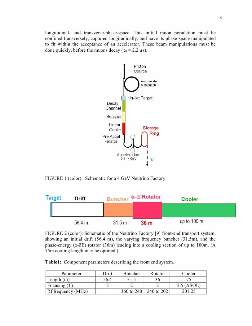
FIGURE 1 (color): Schematic for a 4 GeV Neutrino Factory.

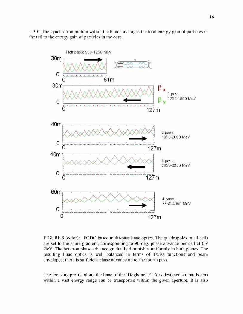
FIGURE 2 (color): Schematic of the Neutrino Factory [9] front-end transport system,

showing an initial drift (56.4 m), the varying frequency buncher (31.5m), and the

phase-energy (-E) rotator (36m) leading into a cooling section of up to 100m. (A

75m cooling length may be optimal.)

Table1: Component parameters describing the front end system.

Parameter Drift Buncher Rotator Cooler

Length (m) 56.4 31.5 36 75

Focusing (T) 2 2 2 2.5 (ASOL)

Rf frequency (MHz) 360 to 240 240 to 202 201.25

4

Rf gradient (MV/m) 0 to 15 15 16

Total rf voltage (MV) 126 360 800

The low energy NF scheme described in this paper is shown in Fig. 1. The

arrangement and lengths of the front-end sections is shown schematically in Fig. 2,

and front-end parameters are listed in Table 1. The Low Energy NF consists of:

i) A proton source producing a high-power multi-GeV bunched proton beam.

ii) A pion production target that operates within a high-field solenoid. The solenoid

confines the pions radially, guiding them into a decay channel.

iii) A ~57m long solenoid decay channel.

iv) A system of rf cavities that capture the muons longitudinally into a bunch train,

and then applies a time-dependent acceleration that increases the energy of the slower

(low energy) bunches and decreases the energy of the faster (high energy) bunches

[16].

v) A cooling channel that uses ionization cooling [17] to reduce the transverse phase

space occupied by the beam, so that it fits within the acceptance of the first

acceleration stages.

vi) An acceleration scheme that accelerates the muons to 4 GeV.

vii) A 4 GeV storage ring with long straight sections.

Schemes for higher energy NFs that have been previously studied are similar in

design up to and including the cooling channel. We have adopted the design from the

recent International Scoping Study [12] (ISS) for the pion production target, decay

channel, and cooling channel. The bunching and phase rotation channel is also similar

to the ISS design, but has an improved optimization of its parameters. The

acceleration and storage ring designs are necessarily different from the ISS design,

and the proton source is taken to be based on the new proton source which is

currently under discussion at Fermilab [18].

3. PROTON SOURCE CONSIDERATIONS

Past studies have shown that, to a good approximation, the number of useful muons

produced at the end of the NF cooling channel is proportional to the primary proton

beam power, independent of the proton beam energy. This is true for proton energies

Ep within the optimal range 5 GeV < Ep < 15 GeV. The number of useful muons per

unit proton beam power falls only slowly above Ep = 15 GeV, and hence proton

sources providing higher energy particles (up to a few tens of GeV) have also been

considered. To obtain sufficient muons per year to meet the physics goals, the ISS

concluded that, with an operational year of only 107 secs, a beam power of 4MW is

required. Previous NF studies [7-11] have also concluded that proton beam powers in

the 2MW to 4MW range are needed. In addition to beam power, NFs also require

5

short proton bunches, specified by the ISS to be 2±1 ns (rms). The phase rotation

scheme described in Section 5 requires that the initial proton bunch length is no

longer than about 3ns (rms). Proton sources that produce longer bunches or too many

bunches will need a rebunching scheme.

More detailed considerations about the proton source needed for a NF can be made in

the context of a specific candidate NF site, and hence an explicit existing or planned

accelerator complex. As an example, in the following we consider the proton source

upgrade plans presently under discussion at Fermilab. The Fermilab Steering Group

has proposed a roadmap [19] for the future of Fermilab that promotes an intensity-

frontier program based on a new high-power H

linac patterned after the International

Linear Collider (ILC) linac design. Initially it was proposed that the new linac would

accelerate the H ions to 8 GeV with an ILC-like beam structure: a beam current of 9

mA lasting for 1 msec at a repetition rate of 5 Hz. That corresponds to 360 kW of

beam power at 8 GeV. However, these specifications are currently under discussion,

and it is expected that the parameter list will be updated to correspond to higher beam

current and power. The 8 GeV beam could be used directly or, after stripping the H

ions at 8 GeV, the Fermilab Main Injector (MI) [20] could be used to accelerate the

protons to higher energy. For example, with appropriate upgrades the MI can

accelerate to about 50 GeV with a 0.6s cycle time. If the 8 GeV linac pulses at 5 Hz,

the Fermilab Recycler ring [21] could be used to accumulate 3 pulses with 5×1013

protons per pulse, allowing the MI to accelerate 1.5×1014

protons to 50 GeV every

0.6s, which corresponds to a beam power of 2 MW. The 50 GeV beam would require

the addition of a Buncher ring to compress the beam to the short bunches needed for

the NF. Note that 2MW is at the low end of what is needed for a NF, and hence

higher beam powers are desirable. With more protons the MI could provide more

beam power and the MI cycle time and energy could be reduced.

In the following we will adopt, as our illustrative baseline scheme, a proton source

that does not use the MI, but achieves high beam power by upgrading the 8 GeV linac

to provide 20 mA for 2.5 ms at 10 Hz. This corresponds to a beam power of ~ 4 MW.

In an operational year of 2 107 sec this would yield 6.3 10

22 protons at 8 GeV.

6

FIGURE 3: Proton rebunching scheme. Accumulator and Buncher rings form intense

short proton bunches. The Combiner is used to adjust the spacing between bunches, if

necessary.

The 8 GeV linac beam must be rebunched to form a bunch structure suitable for a NF.

An illustrative rebunching scheme based on two rings and a bunch combiner is shown

in Fig. 3. The first storage ring (the Accumulator) would accumulate, via charge-

stripping of the H beam, eighteen 100ns long bunches, with each bunch containing

~1.71013

protons. The incoming beam from the linac would be chopped to allow

clean injection into pre-existing RF buckets. Painting will be necessary in the 4-D

transverse phase space, and possibly also in the longitudinal phase-space. Very large

transverse emittances must be created in order to control space-charge forces. The

second storage ring (the Buncher) would accept three bunches at a time from the

Accumulator and then perform a 90 degree bunch rotation in longitudinal phase

space, shortening the bunches just before extraction. Since the momentum spread will

become large, of order 5%, the ring must have a large momentum acceptance1. Also,

when the bunches are short, the space-charge tune shift will be large. Three short

bunches from the Buncher can be extracted with appropriate delays to provide the

desired bunch spacing at the target. Our baseline plan is to use a Combiner transport

scheme to place the three bunches simultaneously on the target.

The Combiner consists of a set of transfer lines and kickers. The first major

subsystem, the “trombone”, sends bunches on paths of different lengths. The second

subsystem, the “funnel”, nestles the bunches side-by-side on convergent paths to the

pion production target. Hence the target would see 5.2 1013

incoming protons six

times per cycle, i.e. every 16.7 msec, (60Hz). The combiner is essential to provide

fewer, more intense bunches for an eventual upgrade to a muon collider. For the NF

we can also consider allowing the bunches to arrive at the target in a closely spaced

sequence, providing three bunches of ’s that would be used to form three closely-

spaced trains of bunches.

Finally, the parameters of the proton beam on target are summarized in Table 2. The

proton source would deliver 6.31022

protons per year at 8 GeV. Note that the

rebunching ideas described here are first concepts. Detailed design studies, beyond

the scope of the present paper, are required to understand the limitations due to space

charge, electron cloud, and other intensity-dependent effects. The design details of the

proton source scenario will also depend on the final form and potential properties of

the upgraded Fermilab proton source. We are however confident that the new linac

could be used as the basis of a multi-MW proton source that can provide the short

multi-GeV proton bunches needed for a NF.

1 Note that the existing 8-GeV Fermilab Accumulator and Debuncher rings in the Antiproton Source are high -quality storage rings that have the right energy and roughly the right circumferences. They are, however, in a shallow tunnel which would limit their high intensity operation. If

relocated to a deeper tunnel they might serve as the Accumulator and Buncher rings in Fig. 3.

7

Table 2: Representative Proton Source parameters. The muon rates are for positive

muons calculated at the end of the muon ionization cooling channel. There will be an

approximately equal number of negative muons.

Linac Beam Properties

Proton Energy Ep (GeV) 8

Cycle Frequency fp (Hz) 10

Current (mA) 20

Pulse Length (ms) 2.5

Proton Beam Power Pp (MW) 4.0

Beam Properties on Target

Repetition Rate f (Hz) 60

Protons/cycle** Np 5.21013

Protons per operational year 2107Np f 6.310

22

Muons per initial 8 GeV proton*) +/p 0.07

Muons per operational year*) +/p210

7Npf 4.410

21

*) At the end of the cooling channel

**) With one bunch per cycle or 3 bunches of 1.71013

4. TARGET AND DECAY CHANNEL

Beam powers of several MW are only of interest if there is also a target technology

that can be used. Recent preliminary results from the Mercury Target experiment

(MERIT [22]) have provided a proof-of-principle demonstration for a target

technology that could survive beam powers of up to ~8MW or higher, which is

adequate for our NF scenario. The target, pion-collection, and pion-decay channel for

high energy Neutrino Factories has been extensively studied in the past. The same

design for these subsystems can be used for a Low Energy NF at an 8 GeV proton

source, and we therefore adopt the design from the ISS [12] which, for completeness,

we summarize in the following.

The 8 GeV proton source produces short pulses of protons which are focused onto a

liquid-Hg-jet target immersed in a high-field solenoid with internal radius rsol. The

bunch length is 1 to 3 ns rms (~5 to 15 ns full-width), Bsol =20T, and rsol = 0.075m.

Secondary particles are radially captured if they have a transverse momentum pT less

than ~ecBsol rsol /2 = 0.225 GeV/c. Downstream of the target solenoid the magnetic

field is adiabatically reduced from 20T to 2T over a distance of ~10m, while the

solenoid radius increases to 0.3m. This arrangement captures within the B=2T decay

channel a secondary pion beam with a broad energy spread (~100 MeV to 300 MeV

kinetic energy).

8

The initial proton bunch is relatively short, and as the secondary pions drift from the

target they spread apart longitudinally: c(s) = s/z + c0, where s is distance along

the transport and z = vz/c is the longitudinal velocity. Hence, downstream of the

target, the pions and their daughter muons develop a position-energy correlation in

the rf-free decay channel. In the baseline design, the drift length LD = 56.4m, and at

the end of the decay channel there are about 0.2 muons of each sign per incident 8

GeV proton [23].

5. BUNCHING AND PHASE ROTATION

The decay channel is followed by a buncher section that uses rf cavities to form the

muon beam into a train of bunches, and a phase-energy rotating section that

decelerates the leading high energy bunches and accelerates the late low energy

bunches, so that each bunch has the same mean energy. The design described below

delivers a bunch train that is 50m long, which is an improvement over the version of

the design developed for the ISS [16, 12] which delivered an 80m long bunch train

containing the same number of muons.

To determine the required buncher parameters, we consider reference particles (1, 2)

at P1= 280 MeV/c and P2 = 154 MeV/c, with the intent of capturing muons in the

corresponding energy range (~80 to ~200 MeV). The rf frequency frf and phase are

set to place these particles at the center of bunches while the rf voltage increases

along the transport. These conditions can be maintained if the rf wavelength rf

increases along the buncher, following:

B rf B

rf 2 1

c 1 1N (s) N s

f (s)

where s is the total distance from the target, 1 and 2 are the velocities of the

reference particles, and NB is an integer. For the present design, NB is chosen to be

10, and the buncher length is 31.5m. With these parameters, the rf cavities decrease

in frequency from ~360 MHz (rf = 0.857m) to ~240 MHz (rf = 1.265m) over the

buncher length.

The initial geometry for rf cavity placement uses 0.5m long cavities placed within

0.75m long cells. The 2T solenoid field focusing of the decay region is continued

through the buncher and the following rotator section. The rf gradient is increased

from cell to cell along the buncher, and the beam is captured into a string of bunches,

each of them centered about a test particle position with energies determined by the

(1/) spacing from the initial test particle:

1/i = 1/1 +n (1/),

where (1/)=(1/2-1/1)/NB. For the present design, the cavity gradients follow a

linear + quadratic increase:

9

B B

2z z

rf L LV (z) 6 9 MV / m ,

where z is distance along the buncher. The gradient at the end of the buncher is 15

MV/m. This gradual increase of the bunching voltage enables a somewhat adiabatic

capture of the muons into separated bunches, which minimizes phase space dilution.

At the end of the buncher, the beam is formed into a train of bunches with different

energies. In the rotator section, the rf bunch spacing between reference particles is

shifted away from the integer NB by an increment NB, and phased so that the high-

energy reference particle would be decelerated and the low-energy one would be

accelerated. For this study NB =0.08 and the bunch spacing between reference

particles NB + NB = 10.08. This is accomplished using an rf gradient of 15 MV/m in

0.5m long rf cavities within 0.75m long cells. The rf frequency decreases from 236

MHz to 202 MHz from cavity to cavity down the length of the 36m long rotator

region.

Within the rotator, the reference particles are decelerated and accelerated at a uniform

rate until, at the end of the channel, their energies become approximately equal. The

particle bunches are then aligned with nearly equal central energies. At the end of the

rotator the rf frequency matches into the rf frequency of the ionization cooling

channel (201.25 MHz). The average momentum at this exit is 230 MeV/c. The

performance of the bunching and phase rotation channel, along with the subsequent

cooling channel, is illustrated in Fig. 4 which shows, as a function of the distance

down the channel, the number of muons within a reference acceptance (muons within

201.25 MHz rf bunches with transverse amplitudes less than 0.03m and longitudinal

amplitudes less than 0.2m). The phase rotation increases the “accepted” muons by a

factor of 4.

A critical feature of the muon production, collection, bunching and phase rotation

system we have described is that it produces bunches of both signs (μ+ and μ

-) at

roughly equal intensities. Note that all of the focusing systems are solenoids which

focus both signs, and the rf systems have stable acceleration for opposite signs

separated by a phase difference of .

10

FIGURE 4 (color): Performance of the bunching and cooling channel as a function of

distance along the channel, as simulated using the ICOOL code [24,25]. The red line

(righthand scale) shows the evolution of the rms transverse emittance. The blue line

(lefthand scale) shows the evolution of the number of muons within a reference

acceptance (muons within 201.25 MHz rf bunches with transverse amplitudes less

than 0.03m and longitudinal amplitudes less than 0.2m). The cooling section starts at

s=124m, where the rms transverse emittance is ~0.017m and ~0.040 /p are in the

reference acceptance, and continues to s = 217m. Acceptance is maximal at 0.085 +

per initial proton at s= 201m (75m of cooling), where the rms transverse emittance is

0.007 m-rad. At s = 173m (59m of cooling) the /p is ~0.072, where the transverse

emittance is ~0.0093m. If the longitudinal acceptance is reduced to 0.15m, the

production is ~0.076 /p at s =201m and ~0.067 /p at s= 173m.

6. COOLING CHANNEL

The cooling channel design from the ISS consists of a sequence of identical 1.5m

long cells (Fig. 5). Each cell contains two 0.5m-long rf cavities, with 0.25m spacing

between the cavities and 1cm thick LiH blocks at the ends of each cavity (4 per cell).

The LiH blocks provide the energy loss material for ionization cooling. Each cell

contains two solenoidal coils of alternating sign; this yields an approximately

sinusoidal variation of the magnetic field in the channel with a peak value of ~2.5T,

providing transverse focusing with 0.8m. The currents in the first two cells are

perturbed from the reference values to provide matching from the constant-field

solenoid in the buncher and rotator sections. The total length of the cooling section is

75m (50 cells). Based on simulations from the ISS, the cooling channel is expected

to reduce the rms transverse normalized emittance from N,rms = 0.018m to N,rms =

0.007m. The rms longitudinal emittance is L,rms = ~0.07 m/bunch.

11

FIGURE 5 (color): Radial cross section of a cooling cell. Note, this design was used

in Neutrino Factory Study 2B [9]. The cooling cell includes two rf cavites, four LiH

absorbers, and two superconducting coils providing ASOL fields.

The effect of the cooling can be measured by counting the number of simulated

particles that fall within a reference acceptance, which approximates the expected

acceptance of the downstream accelerator. As an example, for the Neutrino Factory

study of Ref. [9] particles with transverse amplitudes AT less than 0.03m and

longitudinal amplitudes AL less than 0.15m were considered accepted.

The amplitude AT is given by:

2 2 2 2TA x y x y 2 x x y y 2( L)(x y y x )

where , , are betatron functions, and the last term is an angular momentum

correction [24]. For longitudinal motion the variables tc = c (phase lag in periods

within a bunch multiplied by rf wavelength) and E (energy difference from centroid)

are used (rather than z-z’) and the generalized betatron functions (L, L, L) are

defined in terms of those parameters. The longitudinal amplitude is given by:

2 2L L c L L c2

1A t E 2 t E

(m c )

Note that our notation differs from that in Ref. [9], although the same criteria are

used. Our reference scenario has been simulated using the ICOOL code [25]. Using

the output from our re-optimized buncher and rotator, we have tracked particles

through the ISS cooling channel, and obtain within the reference acceptances at least

12

0.07 μ+ per 8 GeV incident proton

2. The acceptance criteria remove larger amplitude

particles from the distribution, and the rms emittance of the accepted beam is

therefore much less than that of the entire beam. The rms transverse emittance x,y of

the accepted beam is ~4.0 mm-rad. And the rms longitudinal emittance is ~36mm.

At the end of the cooling channel there are interlaced trains of positive and negative

muon bunches. The trains of useable muon bunches are ~50m long (~30 bunches),

with ~70% of the muons in the leading 12 bunches (20m). The bunch length is

~0.16m in c for each bunch with a mean momentum of 230 MeV/c and an rms width

p ≈ 28MeV/c. For the accepted beam, the rms bunch size is <x2>

1/2 = 3.8cm, and the

rms transverse momentum is <px2>

1/2 ≈ 10 MeV/c.

Table 3: Beam emittance/acceptance after the cooling channel at 273 MeV/c. Note

that the longitudinal normalized acceptances defined as 2.5rms.

Parameter rms or

rms

A = (2.5)2

or 2.5rms

Normalized emittance x , y (mm-rad) 4.0 25

Longitudinal emittance

(l = p z / mc)

l (mm) 36 200

Momentum spread p/p 0.1 ±0.25

Bunch length z (m) 0.16 ±0.4

7. ACCELERATION To ensure an adequate survival rate for the short-lived muons, acceleration must

occur at high average gradient. The accelerator must also accommodate the phase-

space volume occupied by the beam after the cooling channel, which is still large [26]

(see Table 3). The need for large transverse and longitudinal acceptances drives the

design of the acceleration system to low RF frequency, e.g. 201 MHz. High-gradient

normal conducting RF cavities at these frequencies require very high peak power RF

sources. Hence Superconducting RF (SCRF) cavities are preferred. In the following

we choose a SCRF gradient of 12 MV/m, which we note has been demonstrated at

201 MHz [27], and which will allow survival of about 84% of the muons as they are

accelerated to 4 GeV.

Our proposed muon accelerator complex consists of (i) an initial 12m long extension

of the cooling channel with the energy absorbers removed so that the channel

accelerates the muons from 230 MeV/c to 273 MeV/c, (ii) a 201 MHz SCRF linac

pre-accelerator that captures the large muon phase space coming from the cooling

channel lattice and accelerates the muons to relativistic energies, while adiabatically

2 We have also studied using 50 GeV incident protons, in which case we obtain ~0.4 + per incident proton.

13

decreasing the phase-space volume, and (iii) a Recirculating Linear Accelerator

(RLA) that further compresses and shapes the longitudinal and transverse phase-

space, while increasing the energy to 4 GeV. The overall layout of the accelerator

complex is shown in Fig. 6.

FIGURE 6: Layout of the accelerator complex. For compactness both components

(the Pre-accelerator and the Dogbone RLA) are stacked vertically; ± beam transfer

between the accelerator components is facilitated by the vertical double chicane (see

text).

7.1 LINEAR PRE-ACCELERATOR

A single-pass linac “pre-accelerator” raises the beam energy to 0.9 GeV. This makes

the muons sufficiently relativistic to facilitate further acceleration in a RLA. In

addition, the longitudinal phase space volume is adiabatically compressed in the

course of acceleration. The large acceptance of the pre-accelerator requires large

aperture and tight focusing at its front-end. Given the large aperture, tight space

constraints, moderate beam energies, and the necessity of strong focusing in both

planes, we have chosen solenoidal focusing for the entire linac. To achieve a

manageable beam size in the linac front-end, short focusing cells are used for the first

6 cryo-modules. The beam size is adiabatically damped with acceleration, and that

allows the short cryo-modules to be replaced with 8 intermediate-length cryo-

modules, and then with 16 long cryo-modules as illustrated in Fig. 7. The initial

longitudinal acceptance of the linac is chosen to be 2.5, i.e. p/p = 17% and RF

pulse length = 73 deg. To perform adiabatic bunching [26], the RF phase of the

cavities is shifted by 72 deg at the beginning of the pre-accelerator and then gradually

changed to zero by the end of the linac. In the first half of the linac, when the beam is

still not completely relativistic, the offset causes synchrotron motion which allows

bunch compression in both length and momentum spread, yielding p/p = 7% and

= 29 deg. The synchrotron motion also suppresses the sag in acceleration for the

bunch head and tail. In our tracking simulation we have assumed a particle

distribution that is Gaussian in 6D phase space with the tails of the distribution

truncated at 2.5, which corresponds to the beam acceptance presented in Table 3.

Despite the large initial energy spread, the particle tracking simulation through the

linac does not predict any significant emittance growth. There is a 0.2% beam loss

coming mainly from particles at the longitudinal phase space boundary. Results of the

0.7 GeV/pass4 GeV

0.9 GeV0.3 GeV

186 m

129 mHighest arc circumference: 225 m

0.7 GeV/pass4 GeV

0.9 GeV0.3 GeV

186 m

129 mHighest arc circumference: 225 m

14

simulation are illustrated in Fig. 8 which shows ‘snapshots’ of the longitudinal phase

space at the beginning, half-way-through, and at the end of the Pre-accelerator.

FIGURE 7: Top: Transverse optics of the linac – uniform periodic focusing with 6

short, 8 medium, and 16 long cryo-modules. Below: Layout of the short, intermediate

and long cryo-modules.

FIGURE 8: Particle tracking results showing adiabatic bunch compression along the

linac. The longitudinal phase-space (z, p/p) is shown before (left), in the middle

(center), and at the end (right) of acceleration.

6 short cryos 8 medium cryos 16 long cryos

1.2 Tesla solenoid 1.3 Tesla solenoid 2.4 Tesla solenoid

15

7.2 MAIN ACCELERATION SYSTEM

The superconducting accelerating structure is expected to be by far the most expensive

component of the accelerator complex. Therefore, maximizing the number of passes in the

RLA has a significant impact on the cost-effectiveness [28] of the overall acceleration

scheme. We propose to use a 4.5 pass ‘Dogbone’ configuration for the RLA (Fig. 6), which

has the following advantages compared to a ‘Racetrack’ configuration:

(i) Better orbit separation at the linac ends resulting from a larger (factor of two) energy

difference between two consecutive linac passes.

(ii) A favorable optics solution for simultaneous acceleration of both + and in which

both charge species traverse the RLA linac in the same direction while passing in the

opposite directions through the mirror symmetric optics of the return ‘droplet’ arcs.

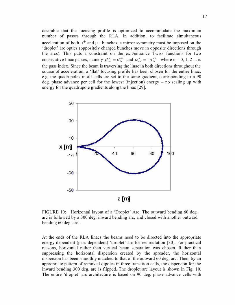
The Dogbone multi-pass linac optics are shown in Fig. 9. The Dogbone RLA simultaneously

accelerates the + and beams from 0.273 GeV to 4 GeV. The injection energy into the

RLA and the energy gain per RLA linac were chosen so that a tolerable level of RF phase

slippage along the linac could be maintained. We have performed a simple calculation of the

phase slippage for a muon injected with initial energy E0 and accelerated by E in a linac of

length L, where the linac consists of uniformly spaced RF cavities phased for a speed-of-light

particle. Our calculation used the following cavity-to-cavity iterative algorithm for the phase-

energy vector:

k,i 2k,i 1

k,ik,i 1

k,i i k,i

h

EE qV cos( )

where h Llinac/Ncav, c/f0, k is the particle index, i 0 … Ncav – 1, and Vi is the maximum

accelerating voltage in cavity i. The resulting phase slippage profiles along the multi-pass

RLA linacs can be summarized as follows. For the RLA injection energy of 0.9 GeV the

critical phase slippage occurs for the initial ‘half-pass’ through the linac and it is about 40º,

which is still manageable and can be mitigated by appropriate gang phase in the following

linac (1-pass). For subsequent passes the phase slippage gradually goes down and can be

used, along with the sizable momentum compaction in the arcs, to further longitudinally

compress the beam. The initial bunch length and energy spread are still large at the RLA

input and further compression is required in the course of the acceleration. To accomplish

this, the beam is accelerated off-crest with non zero momentum compaction (M56) in the

‘droplet’ arcs. This induces synchrotron motion, which suppresses the longitudinal emittance

growth arising from the non-linearity of the accelerating voltage. Without synchrotron

motion the minimum beam energy spread would be determined by the non-linearity of the

RF voltage over the bunch length and would be equal to (1-cos) 9% for a bunch length

16

= 30º. The synchrotron motion within the bunch averages the total energy gain of particles in

the tail to the energy gain of particles in the core.

FIGURE 9 (color): FODO based multi-pass linac optics. The quadrupoles in all cells

are set to the same gradient, corresponding to 90 deg. phase advance per cell at 0.9

GeV. The betatron phase advance gradually diminishes uniformly in both planes. The

resulting linac optics is well balanced in terms of Twiss functions and beam

envelopes; there is sufficient phase advance up to the fourth pass.

The focusing profile along the linac of the ‘Dogbone’ RLA is designed so that beams

within a vast energy range can be transported within the given aperture. It is also

17

desirable that the focusing profile is optimized to accommodate the maximum

number of passes through the RLA. In addition, to facilitate simultaneous

acceleration of both + and bunches, a mirror symmetry must be imposed on the

‘droplet’ arc optics (oppositely charged bunches move in opposite directions through

the arcs). This puts a constraint on the exit/entrance Twiss functions for two

consecutive linac passes, namely 1 n

in

n

out and 1 n

in

n

out where n = 0, 1, 2 ... is

the pass index. Since the beam is traversing the linac in both directions throughout the

course of acceleration, a ‘flat’ focusing profile has been chosen for the entire linac:

e.g. the quadrupoles in all cells are set to the same gradient, corresponding to a 90

deg. phase advance per cell for the lowest (injection) energy – no scaling up with

energy for the quadrupole gradients along the linac [29].

FIGURE 10: Horizontal layout of a ‘Droplet’ Arc. The outward bending 60 deg.

arc is followed by a 300 deg. inward bending arc, and closed with another outward

bending 60 deg. arc.

At the ends of the RLA linacs the beams need to be directed into the appropriate

energy-dependent (pass-dependent) ‘droplet’ arc for recirculation [30]. For practical

reasons, horizontal rather than vertical beam separation was chosen. Rather than

suppressing the horizontal dispersion created by the spreader, the horizontal

dispersion has been smoothly matched to that of the outward 60 deg. arc. Then, by an

appropriate pattern of removed dipoles in three transition cells, the dispersion for the

inward bending 300 deg. arc is flipped. The droplet arc layout is shown in Fig. 10.

The entire ‘droplet’ arc architecture is based on 90 deg. phase advance cells with

18

periodic beta functions. The ‘droplet’ arc optics, which is based on FODO focusing,

[30] is illustrated in Fig. 11 which also shows the longitudinal phase-space occupied

by the beam at the entrance and at the exit of the arc. The momentum compaction of

the arc can be estimated as follows:

tot

rad

dip

xrad

dip

x

dip

x

x DdDs

dDdsD

M

56

FIGURE 11 (color): Top: ‘Droplet’ Arc optics, showing the uniform periodicity of

beta functions and dispersion. Bottom: Particle tracking results showing the

longitudinal phase-space compression. The longitudinal phase-space (s, p/p) is

shown at the beginning (left) and at the end (right) of the arc.

19

Figure 11 shows the momentum compaction is relatively large, which guarantees

significant rotation in the longitudinal phase space as the beam passes through the arc.

This effect, combined with off-crest acceleration in the subsequent linac, yields

further compression of the longitudinal phase-space as the beam is accelerated.

To transfer both + and bunches from one accelerator to the other one, which is

located at a different vertical elevation, we use a compact double chicane based on a

periodic 90 deg. phase advance cell (in FODO style). Each ‘leg’ of the chicane

involves 4 horizontal and 2 vertical bending magnets, forming a double achromat in

the horizontal and vertical planes, while preserving periodicity of the beta functions.

The layout and Twiss functions of the double chicane are illustrated in Fig. 12.

FIGURE 12 (color): Injection Double Chicane. Top: Horizontal and vertical magnet

layout. Middle: Uniformly periodic optics forming a double achromat in the

horizontal and vertical plane. Bottom: Particle tracking results for the longitudinal

phase-space (s, p/p) at the beginning (left) and at the end (right) of the double

chicane.

20

7.3 ACCELERATOR PERFORMANCE

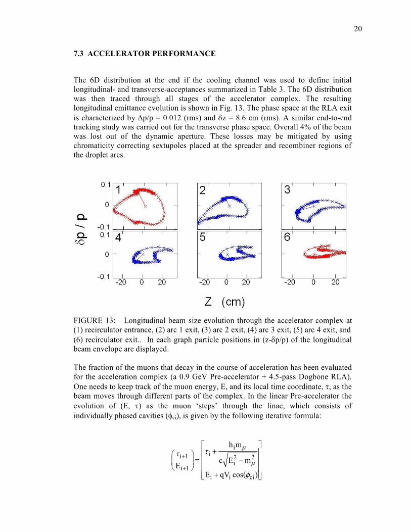
The 6D distribution at the end if the cooling channel was used to define initial

longitudinal- and transverse-acceptances summarized in Table 3. The 6D distribution

was then traced through all stages of the accelerator complex. The resulting

longitudinal emittance evolution is shown in Fig. 13. The phase space at the RLA exit

is characterized by p/p = 0.012 (rms) and z = 8.6 cm (rms). A similar end-to-end

tracking study was carried out for the transverse phase space. Overall 4% of the beam

was lost out of the dynamic aperture. These losses may be mitigated by using

chromaticity correcting sextupoles placed at the spreader and recombiner regions of

the droplet arcs.

FIGURE 13: Longitudinal beam size evolution through the accelerator complex at

(1) recirculator entrance, (2) arc 1 exit, (3) arc 2 exit, (4) arc 3 exit, (5) arc 4 exit, and

(6) recirculator exit.. In each graph particle positions in (z-p/p) of the longitudinal

beam envelope are displayed.

The fraction of the muons that decay in the course of acceleration has been evaluated

for the acceleration complex (a 0.9 GeV Pre-accelerator + 4.5-pass Dogbone RLA).

One needs to keep track of the muon energy, E, and its local time coordinate, , as the

beam moves through different parts of the complex. In the linear Pre-accelerator the

evolution of (E, ) as the muon ‘steps’ through the linac, which consists of

individually phased cavities (ci), is given by the following iterative formula:

iii 1 2 2

ii 1

i i ci

h m

c E mE

E qV cos( )

21

For the RLA linac the formula describing the evolution is simpler since all the

cavities are equally phased (ci = c). Finally, in the arcs the above formula is further

simplified: Vi = 0 (no acceleration). Applying the iterative formulae to all pieces of

the accelerator complex (linacs and arcs) yields the survival rate:

i i0

0 0

Nexp 2.2 s

N

Figure 14 shows the survival rate as a function of energy. The fraction of muons that

survive as they are accelerated to 4 GeV is 84%. Hence, in our scheme, the total

number of muons at the exit of the acceleration system is 3.4 1021

+ per year and a

similar number of (Note: 4 10

21 at the exit of the cooling channel of which 84%

survive to the end of the acceleration).

FIGURE 14 (color): Survival rate as a function of energy; the red and blue lines

show respectively the fraction decaying in the pre-accelerator and RLA. Vertical

drops correspond to the beam transport in arcs .

22

Table 4: Beam parameters at the end of the 4 GeV acceleration system.

rms,

σ

A = (2.5)2

or 2.5σ

Normalized emittance x , y (mm-rad) 5.4 34

Longitudinal emittance

(l = p z / mc)

l (mm) 44 280

Momentum spread p/p 0.012 ±0.03

Bunch length z (mm) 86 ±215

In summary, the results of our study suggest that there are no obvious physical or

technical limitations precluding design and construction of a 4.5-pass ‘Dogbone’

RLA for acceleration of muons to 4 GeV. Design choices made in the proposed

acceleration scheme were driven by the beam dynamics of large phase-space beams.

The beam emittances at the end of the 4 GeV accelerator complex are summarized in

Table 4. At the output of the acceleration system there is a train of 30 bunches per

cycle with the emittances summarized in the table and a bunch spacing of 5 ns. The

total number of 4 GeV muons of each sign per year at the end of the acceleration

system is estimated to be 3.4 1021

.

8. STORAGE RING

Muon decay rings for “high energy” Neutrino Factories have been extensively studied

over the last decade. Both racetrack- (two long straight sections) and triangle- (three

long straight sections) geometries have been proposed. Initial physics studies [14, 15]

suggest that a single baseline would be sufficient for a 4 GeV NF, and hence in the

following we consider a racetrack geometry. In principle both muon signs can be

stored in a single ring in which the μ+ and μˉ bunches are injected in opposite

directions, and both long straight sections point towards the same distant detector.

One straight section provides a neutrino beam from μ+ decays and the other straight

section from μˉ decays. However, for simplicity, we will consider a solution with two

rings, one to store the μ+ and the other to store the μˉ. If the μ

+ bunch trains (in ring

1) are correctly interleaved in time with the counter-rotating μˉ trains (in ring 2) then

the differently charged bunches are not simultaneously travelling towards the far

detector, and hence timing in the far detector can be used to determine whether an

interacting neutrino originated from μ+ or μˉ decay.

Optimally the muon decay rings have circumferences which correspond to an integral

number of proton source cycle times. In our design the neutrino-beam-forming

“production” straight section is constructed from 23m long periodic cells. The

number of cells determines the straight section length which, in practice, could be

chosen to be from 135m to ~500m with corresponding ring circumferences from 500

m to ~1200m, respectively. Note that there are background-sweeping dipoles at each

end of the production straight section, and hence its length is not an exact multiple of

23

23m. The incoming bunch trains are 45m long and are separated by 67ms, hence (a)

the bunch train is much shorter than the production straight, (b) only a single bunch

train is circulating in each ring on any given cycle, and (c) there is plenty of time to

accommodate the rise and fall times of an injection kicker.

The fraction of muons f that decay in the storage ring while traveling in the direction

of the distant detector is determined by the ratio of the production straight section

length to the ring circumference. If the straight section is much longer than the arcs,

fapproaches 0.5. For realistic geometries, f~0.3 - 0.45 seem cost effective. In our

design f = 0.4.

The ring lattice has been designed with the following considerations:

(i) The large transverse beam emittances must be accommodated, and component

apertures must be at least a few centimeters larger than the full beam envelope

(which is ~±11cm maximum in the present arc design using the full

emittances listed in Table 4). Active collimators set to 2.5 sigma will shadow

the arc components and absorb the majority of beam loss. Component

apertures in the arc will therefore be about ±15cm referenced to the central

trajectory. In the production straight section this aperture increases to ±35cm.

(ii) The dynamic aperture must be very large. The lattice arc is based on 90

degree cells which are known to provide large transverse dynamic range even

in the presence of sextupole chromatic correction. The small phase advance

from the production straight section has little impact on overall dynamic

aperture.

(iii) To minimize neutrino flux uncertainties, the rms muon beam divergence in the

production straight section, B, must be much smaller than the rms neutrino

beam divergence, D, arising from the muon decay kinematics. A general

design criteria is that B < 0.1D. In the lattice presented here, B ~ 0.05 D.

Although this seems better than required, the higher beta is desirable since it

allows longer spacing between the quadrupoles in the production straight

section, reducing significantly the number of components. Permanent magnets

can be used, and hence the large quadrupole apertures that are needed (70cm)

are not a consideration.

(iv) A background-sweeping dipole must be incorporated at the ends of the

straight sections to minimize end-effects which contribute to the neutrino flux

uncertainties. These magnets complicate the lattice designs by creating

dispersion in the high beta regions of the production straight section. In our

lattice, strong dispersion is first canceled with two dispersion suppression

cells at the entrance/exit of each arc. Two weaker dipoles are paired in the arc

matching section and the beginning of the production straight section to

simultaneously sweep backgrounds and cancel dispersion through the

production straight section.

24

(v) The ring must accommodate the muon beam momentum spread which, after

acceleration, is (p/p) = 0.03. A sufficiently large momentum acceptance

requires chromaticity correction through the use of sextupoles.

Table 5: Decay Ring parameters.

Arc cell length 8

#arc cells 16

#dispersion suppressor

cells

8

max (arc) 13 m

max (straight section) 120m

Straight section length 200m

x /y per cell 90 / 90

magnet spacing 0.5 m

Dx max 2.0 m

Strong focusing FODO cells were chosen for the arcs to achieve a large momentum

acceptance. The chosen racetrack design has two identical arcs each with 8 FODO

cells of fixed-field dipole and quadrupole magnets. Two dispersion suppression cells

are located at each end of the arcs and are identical with respect to the quadrupoles,

although they have different dipole strengths to suppress the strong dispersion outside

of the production straight section. For a 90 cell lattice, each of dispersion cells

would have half the bend strength of an arc cell. A 90 phase advance per cell was

chosen to support strong sextupole correction of linear chromaticity while

simultaneously maintaining an acceptable transverse acceptance. Poletip fields in the

strong arc quadrupoles reach just under 1.5 T, and the dipole bending field is ~1.05T,

so permanent magnets for the entire lattice are an attractive possibility. Table 5

provides an overall summary of the design, and Fig. 15 shows optical functions for

the magnet arc cell. Fig. 16 shows optical functions for the neutrino beam-forming

straight section. The rms muon beam divergence in the straight section is 0.05D.

With an emittance of 34 mm-rad and a of ~100m, the full beam size is ±30cm

(2.5). Despite large apertures, these quadrupoles maintain a poletip field of < 2 kG,

allowing the use of relatively weak permanent magnets and eliminating the need for

significant magnet utilities in the long production straight sections. Somewhat

smaller beta-functions can be tolerated and still meet the divergence criterion, but

25

more magnets would be required in the straight sections3. The main lattice

components comprising the NF ring can be implemented using permanent magnets,

although aircore trim magnets will be required for tune and steering adjustments. A

70cm circular bore could be used to connect the arcs without requiring significant

utilities or services.

FIGURE 15 (color): Optical functions (x, y, Dx) for the permanent magnet arc cell,

which consists of 4 1m dipoles and 2 0.5m quadrupoles, with 0.5 m spacing between

magnets. The magnets would have an aperture of ~0.15m radius.

3 Reducing the beta by a factor of 4, to the 0.1 limit, would require approximately doubling the number of magnets in the production straight

section. The only advantage is that the magnet aperture, but not the strength, would dr op to ±15cm, comparable to the arc magnets. This would

allow a 30cm circular bore to be used for the arcs.

26

Figure 16 (color): Optical functions (x, y, Dx) for the half ring showing the beam -

forming straight section between arc sections, and contrasting the weak -focusing

straight sections with the stronger focusing arcs of the racetrack lattice.

9. DETECTOR CONSIDERATIONS

To fully exploit the rich neutrino oscillation pattern that can be obtained at the low

energy NF, the detector must:

(i) Have high detection efficiency for neutrinos with interaction energy at or

above ~0.5 GeV.

(ii) Have excellent energy resolution.

(iii) Be capable of determining the sign of muons with momentum as low as 0.5

GeV/c and do it with a very low charge mis-ID rate, and therefore be

magnetized.

The detector concept [11] is a magnetized totally active scintillator detector (TASD).

A first study of the performance of this design is presented in the ISS report. Further

details describing its simulated performance are given in [13]. For completeness, we

briefly describe the detector and its expected performance in the following.

27

FIGURE 17 (color): Magnetic cavern concept for a 22.5 Kton fiducial mass low

energy NF detector.

The totally active scintillator neutrino detector concept is not new. Kamland [31] has

been operating for a number of years already and the the Nova Collaboration [32] is

proposing to build a 15-18 kT liquid scintillator detector to operate off-axis to the

NuMI [33] beam line at Fermilab. However, the proposed low energy NF TASD

would have a segmentation that is approximately 10 that of Nova and be

magnetized. Magnetization of such a large volume (>20,000 m3) is the main

technical challenge of this detector design, although R&D to reduce the detector cost

(driven in part by the large channel count, 7.5106) is also needed. The detector

would consist of long scintillator bars with a triangular cross-section arranged in

planes which make x and y measurements. The scintillator bars have a length of 15m

and triangular cross-section with a base of 3cm and a height of 1.5cm. This design is

an extrapolation of the MINERA experiment [34] which in turn was an

extrapolation of the D0 preshower detectors [35]. A TASD detector fiducial mass of

approximately 22.5 Kton has been considered with dimensions 15 15 100 m3.

We believe that an air-core solenoid can produce the field required (0.5 Tesla) to do

the physics. Producing the large magnetic volume presents a formidable technical

challenge. Conventional superconducting magnets are believed to be too expensive

due to the cost of the enormous cryostats needed. In order to eliminate the cryostat it

is proposed to use an unconventional design based on the superconducting

transmission line (STL) that was developed for the Very Large Hadron Collider

superferric magnets

[36]. The solenoid windings would consist of this

superconducting cable which is confined in its own cryostat. To accommodate the

TASD volume, a magnetic cavern containing ten solenoids could be built, each

consisting of 150 turns and ~7500 m of cable. The concept is illustrated in Fig. 17. A

simulation [37] of the Magnetic Cavern concept using STL solenoids has been

performed. With the iron end-walls (1m thick), the average field in the xz-plane is

approximately 0.58 T at an excitation current of 50 kA. The detector has been

28

simulated using the GEANT4 code (version 8.1). The simulation results suggest that a

totally active scintillator detector within a 0.5T magnetic cavern is an attractive

concept for a low energy NF detector, and would enable neutrino interctions to be

measured, with good precision and efficiency, down to energies of ~0.5 GeV. Above

0.5 GeV the detector has a simulated energy-independent efficiency of 0.73, the loss

arising primarily from neutrino interaction kinematics.

Based on the simulated performance of the detector, and of our low energy NF

design, we would expect the resulting neutrino experiment to have a sensitivity that

corresponds to 3 1022

Kt-decays per operational year (assumed to be 2 107 secs of

accelerator up-time) for each muon sign (6 1022

Kt-decays/yr total). Physics

sensitivities have been described in [15] for a neutrino oscillation experiment at a 4

GeV NF and datasets that for each muon sign correspond to 1 1023

Kt-decays and 3

1023

Kt-decays. These datasets could be obtained at the NF we have described in

this paper with respectively 3.3 years and 10 years of data taking.

10. SUMMARY

We have studied a promising design for a low energy NF that would produce neutrino

beams generated by 1.4 1021

+ per year decaying in the long straight section of

storage ring, and a similar number of decays. The design is based upon (i) an

4MW proton source (for example, an upgraded version of the 8 GeV Project X linac

under discussion at FNAL), (ii) the ISS target and decay channel, bunching and phase

rotation channel design, with a re-optimization of the bunching and phase rotation

channel that reduces its length whilst maintaining its performance, (iii) the ISS muon

cooling channel, (iv) an acceleration system that consists of an initial linac pre-

accelerator followed by a “dogbone” RLA, and finally (v) a permanent magnet

storage ring with long straight sections.

ACKNOWLEDGMENTS

This work is supported at the Fermi National Accelerator Laboratory, which is

operated by the Fermi Research Alliance, LLC, under contract No. DE-AC02-07CH11359 with the U.S. Department of Energy.

REFERENCES

[1] B.~T. Cleveland et al., “Measurement Of The Solar Electron Neutrino Flux With

The Homestake Chlorine Detector”, Astrophys. J. 496, 505 (1998); Y. Fukuda

et al. (Kamiokande Collaboration), “Solar neutrino data covering solar cycle

22”, Phys.\ Rev. Lett. 77, 1683 (1996); J. N. Abdurashitov et al. (SAGE

Collaboration), “Measurement of the solar neutrino capture rate by the Russian-

American gallium solar neutrino experiment during one half of the 22-year

29

cycle of solar activity”, J. Exp. Theor. Phys. 95, 181 (2002); W. Hampel et al.

(GALLEX Collaboration), “GALLEX solar neutrino observations: Results for

GALLEX IV”, Phys.\ Lett.\ B {\bf 447}, 127 (1999); T. A. Kirsten (GNO

Collaboration), “Progress in GNO”, Nucl. Phys. Proc. Suppl. 118, 33 (2003).

S.~Fukuda et al. (Super-Kamiokande Collaboration), “Determination of solar

neutrino oscillation parameters using 1496 days of Super-Kamiokande-I data”,

Phys.\ Lett. B539, 179 (2002); Q. R. Ahmad et al. (SNO Collaboration),

“Measurement of the charged current interactions produced by B-8 solar

neutrinos at the Sudbury Neutrino Observatory,'' Phys. Rev. Lett. 87, 071301

(2001); Q. R. Ahmad et al. (SNO Collaboration), “Direct evidence for neutrino

flavor transformation from neutral-current interactions in the Sudbury Neutrino

Observatory”, Phys. Rev. Lett. 89, 011301 (2002); S. N. Ahmed et al. (SNO

Collaboration), “Measurement of the total active B-8 solar neutrino flux at the

Sudbury Neutrino Observatory with enhanced neutral current sensitivity”, Phys.

Rev. Lett. 92, 181301 (2004); B. Aharmim et al. (SNO Collaboration),

“Electron energy spectra, fluxes, and day-night asymmetries of B-8 solar

neutrinos from the 391-day salt phase SNO data set”, Phys. Rev. C72, 055502

(2005).

[2] Y. Ashie et al. (Super-Kamiokande Collaboration), “A measurement of

atmospheric neutrino oscillation parameters by Super-Kamiokande I”, Phys.

Rev. D71, 112005 (2005).

[3] K. Eguchi et al. (KamLAND Collaboration), “First results from KamLAND:

Evidence for reactor anti-neutrino disappearance”, Phys. Rev. Lett. 90, 021802

(2003).

[4] M. H. Ahn (K2K Collaboration), “Measurement of neutrino oscillation by the

K2K experiment”, Phys. Rev. D74, 072003 (2006); D. G. Michael et al.

(MINOS Collaboration), Phys. Rev. Lett. 97, 191801 (2006).

[5] S. Geer, “Neutrino beams from muon storage rings: Characteristics and physics

potential”, Phys. Rev. D57 (1998) 6989.

[6] S. Geer and H. Schellman (Eds), “Physics at a Neutrino Factory”, FERMILAB-FN-

692, hep-ex/0008064; A.D. Rujula, M.B. Gavela, P. Hernandez, Nucl. Phys. B547

(1999) 21; S.F. King, K. Long, Y. Nagashima, B.L. Roberts, O. Yasuda (Eds),

“Physics at a future Neutrino Factory and super-beam facility: Summary of the

Physics Working Group”, RAL-TR-2007-019, December 2007.,

arXiv:0712.4129v2 [hep-ph] 23 Nov 2007.

[7] N. Holtkamp and D. Finley, eds., “A Feasibility Study of a Neutrino Source based

on a Muon Storage Ring”, Fermilab-Pub-00/108-E (2000).

[8] S. Ozaki, R. Palmer, M. S. Zisman, Editors, “Feasibility Study-II of a Muon-

Based Neutrino Source”, BNL-52623, June 2001.

http://www.cap.bnl.gov/mumu/studyII/FS2-report.html.

[9] S. Geer and M. Zisman (Eds), “The neutrino factory and beta beam experiments

and development”, APS Neutrino Study, BNL-72369-2004, FERMILAB-TM-

2259, Nov 2004. 115pp. , e-Print: physics/0411123

[10] S. Geer and M.S. Zisman, “Neutrino Factories: Realization and physics

potential”, Prog. in Part. and Nucl. Physics 59 (2007) 631.

30

[11] J. S. Berg, S. A. Bogacz, S. Caspi, J. Cobb, R. C. Fernow, J. C. Gallardo, S.

Kahn, H. Kirk, D. Neuffer, R. Palmer, K. Paul, H. Witte, M. Zisman, “Cost -

effective Design for a Neutrino Factory”, Phys. Rev. STAB 9,011001(2006).

[12] J.S. Berg et al. (ISS Accelerator Working Group), “International scoping study

of a future Neutrino Factory and super-beam facility: Summary of the

Accelerator Working Group”, (ed. M. Zisman), RAL-TR-2007-23, December

2007; arXiv:0802.4023v1 [physics.acc-ph], 27 February 2008.

[13] T. Abe et al. (ISS Detector Working Group), “International scoping study of a

future Neutrino Factory and super-beam facility: Summary of the Detector

Working Group”, RAL-TR-024, December 2007., arXiv:0710.4947v1

[physics.ins-det] 26 Dec 2007.

[14] S. Geer, O. Mena, S. Pascoli, “Low energy neutrino factory for large 13.”, Phys.

Rev. D 75, 093001 (2007)

[15] A. Bross, M. Ellis, S. Geer, O. Mena, S. Pascoli, “Neutrino factory for large and

small 13.”, Phys. Rev. D 77, 093012 (2008)

[16] D. Neuffer and A. Van Ginneken, Proc. 2001 Particle Acc. Conf. , Chicago, p.

2029 (2001), D. Neuffer, “‘High Frequency’ Buncher and Phase Rotation”,

Proc. NuFACT03, AIP Conf. Proc. 721, p. 407. (2004).

[17] A.N. Skrinsky and V.V. Parkhomchuk, Sov. J of Nuclear Physics 12, 3 (1981);

D. Neuffer, Particle Accelerators 14, 75 (1983).

[18] D. McGinnis, “A 2 MegaWatt Multi-Stage Proton Accumulator”, Fermilab

Beams-Doc-1782, November 2005.

[19] Fermilab Steering Group report,

http://www.fnal.gov/pub/directorate/steering/pdfs/SGR_2007.pdf

[20] D. Neuffer, “Parameters for a Project -X based Muon Collider”, MuCOOLnote

517, March 2008.

[21] Fermilab Recycler Ring Technical design report, Fermilab-TM-1991, November

1996.

[22] H. G. Kirk et al., “A high-power target experiment at the CERN PS,” in Proc.

2007 Particle Accelerator Conf., Albuquerque, June 25–29, 2007, pp. 646–648.

[23] N. Mokhov, “Particle Production and Radiation Environment at a Neutrino

Factory Target Station”, Fermilab-Conf-01/134, Proc. 2001 Particle Accelerator

Conference, Chicago, P. 745 (2001), see http://www-ap.fnal.gov/MARS/

[24] R. Fernow, “Physics Analysis Performed by ECALC9”, Mucool Note 280,

September 2003.

[25] R. Fernow, “ICOOL, a Simulation Code for Ionization Cooling of Muon

Beams”, Proc. 1999 Particle Accelerator Conference, New York, p. 3020

(1999), see http://pubweb.bnl.gov/people/fernow/.

[26] S.A. Bogacz, Journal of Physics G: Nuclear and Particle Physics, 29, 1723,

(2003)

[27] B Autin et al 2003 J. Phys. G: Nucl. Part. Phys. 29 1637-1647.

[28] J.S. Berg et al., Physical Review Special Topics – Accelerators and Beams, 9,

011001 (2006)

[29] S.A. Bogacz, Nuclear Physics B, Vol 149, 309, (2005).

[30] S.A. Bogacz, Nuclear Physics B, Vol 155, 334, (2006) .

31

[31] K. Eguchi et. al., `”First Results from KamLand: Evidence for Reactor

Antineutrino Disappearance,” Physical Review Letters, 90, No. 2, January, 2003.

[32] Ayres et. al., Nova Technical Design Report, May, 2007.

[33] J. Hylen et al., FERMILAB-TM-2018, (1997), “Conceptual design for the technical

components of the neutrino beam for the main injector (NuMI)”.

[34] K. S. McFarland, “The MINERvA experiment at FNAL,” Eur. Phys. Journal A

24S2, 187 (2005).

[35] P. Baringer et. al., “Cosmic-ray Tests of the D0 preshower detector”, Nucl.

Instrum. Meth A469, 2001.

[36] Ambrosio et. al, “Design Study for a Staged Very Large Hadron Collider,”

Fermilab-TM-2149, June, 2001.

[37] V. Kashikhin, private communication