low impact development manual for arkansas

Low Impact Development Manual for

Arkansas

Produced by Marty Matlock, PhD, P.E. C.S.E Area Director, Center for Agricultural and Rural Sustainability Rusty Tate, M. Sc. Eng. Zara Niederman, M.C.P. Sarah E. Lewis, B.S. Ed., M.A. John Metrailer, B.S.

May 20, 2010

i

Contents Chapter 1: Low Impact Development Introduction .................................................................................. 1

1.1 Hydrology ...................................................................................................................................... 1

1.2 Low Impact Development .............................................................................................................. 4

1.2.1 Bioretention Facilities ............................................................................................................. 4

1.2.2 Detention Basins ..................................................................................................................... 5

1.2.3 Vegetated Systems .................................................................................................................. 6

1.2.4 Infiltration Trench ................................................................................................................... 6

1.2.5 Pervious Pavement ................................................................................................................. 6

1.2.6 Rainwater Harvesting .............................................................................................................. 7

1.3 References ..................................................................................................................................... 7

Chapter 2: Stormwater Modeling .......................................................................................................... 12

2.1 Stormwater Model Review........................................................................................................... 12

2.1.1 EPA-SWMM 5.0 – Stormwater Management Model .............................................................. 12

2.1.2 PondPack .............................................................................................................................. 15

2.1.3 CivilStorm ............................................................................................................................. 16

2.2 References ................................................................................................................................... 16

Chapter 3: LID in Arkansas: The Determinants ....................................................................................... 18

3.1 Climate ........................................................................................................................................ 18

3.1.1 Rainfall .................................................................................................................................. 18

3.2 Earth Resources ........................................................................................................................... 20

3.2.1 Geology/Soils ........................................................................................................................ 20

3.2.2 Hydrologic Soil Groups .......................................................................................................... 22

3.2.3 Biotic Resources .................................................................................................................... 24

3.3 Sensitive Areas............................................................................................................................. 27

3.3.1 Wetlands .............................................................................................................................. 27

3.3.2 Wellhead Protection Areas/Public Water Supply ................................................................... 27

3.3.3 Sensitive Waters ................................................................................................................... 28

3.4 References ................................................................................................................................... 30

Chapter 4: LID Best Management Practices ........................................................................................... 31

ii

4.1 Underground Detention ............................................................................................................... 31

4.2 Infiltration Basin .......................................................................................................................... 32

4.3 Rainwater Harvesting ................................................................................................................... 33

4.4 Vegetated Filter Strip ................................................................................................................... 35

4.5 Pervious Pavement ...................................................................................................................... 36

4.6 Vegetated Roof ............................................................................................................................ 38

4.7 Tree Box Filters ............................................................................................................................ 39

4.8 Infiltration Trench ........................................................................................................................ 40

4.9 Constructed Wetland ................................................................................................................... 42

4.10 Oversized Pipe ........................................................................................................................... 43

4.11 Dry Pond .................................................................................................................................... 45

4.12 Wet Pond ................................................................................................................................... 46

4.13 Riparian buffer ........................................................................................................................... 47

4.14 Bioretention Device ................................................................................................................... 49

4.15 Flow Control Devices.................................................................................................................. 50

4.16 Wet Vault .................................................................................................................................. 52

4.17 Erosion Control Device ............................................................................................................... 53

4.18 Vegetated Swale ........................................................................................................................ 54

4.19 Sand Filters (Surface and Underground) ..................................................................................... 55

4.20 References ................................................................................................................................. 57

Chapter 5: Case Study: Implementation of Low Impact Development Best Management Practices to

Control Sediment from Urban Development in Fayetteville, AR ............................................................. 59

5.1 Introduction ................................................................................................................................. 59

5.2 Problem Statement ...................................................................................................................... 59

5.3 Site Conditions ............................................................................................................................. 60

5.4 Modeling: SWMM and SUSTAIN Models ...................................................................................... 61

5.4.1 Modeling College Branch in SWMM ...................................................................................... 62

5.4.2 SWMM Modeling Assumptions ............................................................................................. 62

5.5 SWMM Modeling Results ............................................................................................................. 64

5.5.1 Total Runoff and TSS ............................................................................................................. 64

5.5.2 Model Storm Runoff and TSS ................................................................................................. 65

5.6 Discussion .................................................................................................................................... 66

iii

5.7 References....................................................................................................................................... 67

5.8 Appendix A: Maps ............................................................................................................................ 68

5.9 Appendix B. SWMM Modeling Subwatersheds and BMPs ................................................................ 83

5.10 Appendix C. SWMM Modeling Hydrographs .................................................................................. 85

1

Chapter 1: Low Impact Development Introduction

1.1 Hydrology

Hydrology is the study of water and its properties, distribution, and effects on earth as it

cycles though earth’s surface, subsurface, and atmosphere (McCuen, 2005). The hydrologic

cycle (Figure 1) visually defines the naturally occurring processes that manage water.

Thornthwaite and Mather (1957) summarized the hydrologic cycle using the water budget

equation

P = R + I + ET + S

where P = precipitation, R = surface water runoff, I = infiltration into the soil and ultimately the

groundwater table, ET = evaporation to the atmosphere plus the transpiration or water loss by

plants, and S = change in storage. Infiltration, evapotranspiration, and change in storage are

considered to be abstractions to precipitation meaning these losses do not show up as

stormwater runoff therefore the volume of stormwater runoff can be approximated by

subtracting the abstractions from the volume of precipitation (Hann et al., 1994).

Precipitation is the hydrologic cycle component that initiates stormwater runoff (Davis

& Cornwell, 2008). As precipitation falls, it will ultimately fall onto either a pervious or an

impervious surface. Undisturbed watersheds are predominantly comprised of pervious

surfaces, therefore precipitation that reaches the ground is stored, absorbed, and/or volatilized

through ponding, infiltration, and evapotranspiration. Through these processes pollutants are

removed and surface runoff is minimized (Coffman et al, 1999). However, urban watersheds

are dominated by concentrated areas of human activity and are primarily composed of

impervious surfaces which practically eliminate the natural processes that manage stormwater.

This results in increased runoff volumes and peak flows as well as shorter times of

concentration (Leopold, 1968; Burns et al., 2005) as shown in Figure 2.

2

Figure 1: Hydrologic Cycle

Source: Vesilind et al., 2010

The biggest problem associated with urbanization is the increase of impervious surfaces.

Lee and Heaney (2003) contend that directly connected impervious surfaces should be used as

the key indicator of urbanization in regards to its effects on stormwater instead of total

impervious area. Theobold et al. (2009) estimated 83,479 km2 of impervious surfaces across

the United States as of 2000 and predicted a 36.2% increase by the year 2030. The conversion

of land previously managed for agricultural uses to impervious surfaces is a major controlling

factor in the hydrologic cycle (Pappas et al., 2008).

Figure 2: Pre-development and Post-development Runoff Hydrographs

3

Altering one component of the hydrologic cycle will no doubt cause changes in the other

components as shown by the water budget equation. As infiltration along with surface and

groundwater storage decreases, stormwater runoff volume and rate invariably increases. In a

typical eastern hardwood forest, about 40% of the annual water budget is accounted for

through evapotranspiration, 50% as subsurface flows, and less than 10% as stormwater runoff.

However, after development, stormwater runoff now accounts for up to 43% of the annual

water balance while subsurface flow is reduced to 32% and evapotranspiration rates are

reduced to 25% (Prince George’s County, 1999a).

Changes in impervious cover impact both surface or stormwater runoff quantity as well

as water quality (Glick, 2009). Huang et al. (2008) developed a diagram with peak ratios

expressed as a function of return periods along with impervious percentages. Figure 3 shows

that as the percentage of impervious cover increases, the peak ratio also increases. Kaufmann

et al. (2009) found a correlation between increased impervious cover and decreased stream

base flow and also noted the potential impacts on drinking water and aquatic resource flow

during drought periods. Increased impervious cover has also been shown to alter the hydrology

and geomorphology of streams as well as lead to discharges of stormwater runoff with

increased loading of nutrients and other contaminants (U.S. EPA, 1993; Schueler, 1994; Paul

and Meyer, 2001).

Figure 3: Increasing ratio of peak flow from the natural status to the urban status.

Source: Huang et al., 2008.

4

1.2 Low Impact Development

“Low Impact Development (LID) is an approach to land development that uses various

land planning and design practices and technologies to simultaneously conserve and protect

natural resource systems and reduce infrastructure costs “(HUD, 2003). The focus of this

discussion will be on the applicability of LID as an alternative approach to stormwater

management. LID was piloted in Maryland “as a way to mitigate the negative effects of

increasing urbanization and impervious surfaces” (Dietz, 2007). The overall goal of LID is to

control stormwater at the source by creating a hydrological functional landscape that mimics

the predevelopment or natural hydrology of a given area. This is achieved through a variety of

mechanisms such as infiltration, ponding, interception, and evapotranspiration using Best

Management Practices (Coffman et al, 1999).

Best Management Practices (BMPs) are design techniques that are used to achieve the

desired post development hydrologic conditions. BMPs can be considered either non-structural

or structural. Non-structural BMPs are practices designed to limit the generation of storm

water runoff or reduce the amounts of pollutants contained in the runoff. While structural

BMPs are engineered and constructed systems that improve the quality and control the

quantity of stormwater (US EPA, 1999). Some common non-structural BMPs used in LID are

disconnected impervious areas, cluster development, minimization of soil compaction, and

minimization of total disturbed area. Structural BMPs include bioretention facilities, detention

basins, vegetated systems, infiltration trenches, pervious pavements, and rainwater harvesting

(SEMCOG, 2008; Prince George’s County, 1999b).

1.2.1 Bioretention Facilities

Bioretention is a “water quality and water quantity control practice using the chemical,

biological, and physical properties of plants, microbes, and soils for the removal of pollutants

from stormwater runoff” (Prince George’s County, 2007). Bioretention facilities are shallow

surface depressions that contain layers of organic, sandy soil and mulch as well as surface

vegetation. The most common type of a bioretention facility is a rain garden. Runoff volumes

are reduced by the physical processes of infiltration and retention. While pollutants are

removed through adsorption, plant uptake, decomposition, etc. (US EPA, 1999a).

Many studies have shown bioretention to be effective not only at removing pollutants

but also at runoff volume and peak flow reduction. Studies have shown a high removal

efficiency for total suspended solids and metals but the removal efficiencies for nutrients such

as nitrogen and phosphorous have been highly variable, likely due to the complexity of the

chemistry of these species (Davis et al., 2009; Hatt et al., 2009). Dietz and Clausen (2008) found

5

that the removal rate for total phosphorous was a 110% increase, indicating that more

phosphorous left the system than entered while the mass removal rate for total nitrogen was

32% removal at the bioretention sites in Haddam, CT.

Hunt et al. (2006) reported that estimated annual total nitrogen mass removal was 40%

and mass removal rates for total phosphorous ranged from 65% removal to a 240% increase at

bioretention field sites in North Carolina. These bioretention cells also reduced the mass of

heavy metals in the outflow to a very high degree. Mass removal rates for copper and zinc

were found to be more than 98% and lead removal rates exceeded 80%. Additional studies

have shown similar results for the use of bioretention to remove metals in stormwater

(Rosseen et al., 2006; Ermilio, 2005). Davis (2008) reported peak flow reductions of 44-63% as

well as delayed flow peaks at bioretention facilities constructed at the University of Maryland.

Hatt et al. (2009) found that bioretention devices attenuate peak runoff rates by 80% and

reduce runoff volumes by 33% on average.

1.2.2 Detention Basins

Detention basins are stormwater structures that provide temporary storage of

stormwater runoff in order to prevent downstream flooding (SEMCOG, 2008). Detention basins

may be dry ponds, wet ponds, or constructed wetlands. Their primary purpose is to attenuate

stormwater flow which leads to a reduction of peak runoff rates. A secondary purpose for

detention basins is pollutant removal. Dry ponds are effective at removing sediment. Wet

ponds and constructed wetlands not only remove sediment, but they also remove other

pollutants through biological uptake processes. Average long term pollutant removal rates for

different types of detention basins are shown in Table 1 (Winer, 2000).

Table 1: Median Pollutant Removal Rates

Pollutant Dry Pond Wet Pond Constructed

Wetlands

TSS 47% 80% 76%

TP 19% 51% 49%

TN 25% 33% 30%

Source: Winer, 2000.

6

1.2.3 Vegetated Systems

Vegetated systems such as vegetated filter strips and vegetated swales are used for

conveying and treating stormwater flows (USEPA, 1999b). A vegetated filter strip is a

permanent, maintained strip of vegetation designed to slow runoff velocities and filter out

sediment and other pollutants from urban stormwater (SEMCOG, 2008). Filter strips have

dense vegetation which allows it to filter, slow, and infiltrate sheet flow. They are usually

located between pollutant source areas and a downstream receiving water body. Vegetated

swales are broad, shallow channels planted with vegetation and designed to slow runoff,

promote infiltration, and filter pollutants while conveying stormwater (SEMCOG, 2008).

Fletcher et al (2002) found vegetated swales to be an effective stormwater treatment

measure, providing a substantial reduction in pollutant concentration. Pollutant reduction

ranged from 73 to 94% for TSS, 44 to 57% for TN, and 58 to 72% for TP. However, the

treatment performance diminished with increasing flow, especially for TSS removal. Fletcher

noted that results were within the range reported by the literature. Studies conducted by the

University of New Hampshire Stormwater Center (2008) found removal efficiencies for TSS to

be 60%, 88% for Petro Hydrocarbons, and 88% for zinc. They also found annual average peak

flow reductions of 48%.

1.2.4 Infiltration Trench

An infiltration trench is an excavated trench that has been back filled with stone to form

a subsurface basin (Prince George’s County, 1999b). Infiltration trenches are designed to store,

capture, and infiltrate runoff into the surrounding soils. The removal performance of

infiltration trenches has not been thoroughly reported which is most likely due to the difficulty

in determining the quality of the effluent. The data that are available vary drastically due to

many factors such as varying soil conditions, depth to water table, etc (Weiss et al., 2007). A

study by Weiss (2005) reports assumed values of 75% and 55% for TSS and phosphorous

removal respectively.

1.2.5 Pervious Pavement

Pervious pavement is an infiltration technique that combines stormwater infiltration,

storage, and structural pavement. Paving consists of a permeable surface which may include a

subsurface base made of course aggregate. It provides pre-treatment by removing sediment

and other pollutants. Variations of pervious paving designs include manufactured permeable

paver blocks, porous asphalt, pervious concrete, and gravel. Pervious paving reduces the

amount of impervious surface area for a site (SEMCOG, 2008; US EPA, 1999c).

7

Permeable pavements allow for reductions in runoff quantity and peak runoff rates

because of their ability to allow water to quickly infiltrate through the surface (Collins et al.,

2007; Bratteo and Booth, 2003; Briggs, 2006). Gilbert and Clausen (2006) compared runoff

from traditional asphalt, pavers, and crushed stone. The reduction in runoff from asphalt to

paver surface was 72% and to crushed stone was 98%. Permeable pavements also affect the

water quality of runoff and they have been shown to cause significant decrease in pollutant

concentrations, most notably in total suspended solids (TSS) and heavy metals such as zinc

(Brattebo and Booth, 2003; Gilbert and Clausen, 2006). A study by Briggs (2006) on porous

asphalt reported a 99% median removal efficiency for TSS and a 96% median removal efficiency

for zinc. The removal efficiencies are consistent with other reported values in literature

(USEPA, 1999c; UNHSC, 2007)

1.2.6 Rainwater Harvesting

Rainwater harvesting systems are designed to intercept and store runoff from rooftops

and other impervious surfaces. Rainwater harvesting allows for the water to be reused which

reduces runoff volume therefore having less impact on water quality. Rain barrels are one

variation of rainwater harvesting systems. Rain barrels are often used at individual residences

and the water is reused for garden irrigation. Another variation is a cistern. Cisterns are

generally larger than rain barrels and used for water supply, rather than irrigation (SEMCOG,

2008).

Besides water reuse, rainwater harvesting systems can also be used to control runoff

rates by reducing the runoff volume. Schneider and McCuen (2006) used peak discharge

reduction, trap efficiency, and volume reduction as the hydrologic criteria to evaluate the

effectiveness of cisterns. Their results for peak discharge reduction showed that cisterns were

very effective for small storms and ineffective for large storms. For mid-volume storm events,

the results were variable, but still effective. A study by Gilroy & McCuen (2009) concluded that

“the effectiveness of cisterns in controlling flood runoff lessens as the size of the storm

increases”. They found that for a 1-yr storm event on a single family lot, cisterns reduced the

peak rate and volume by 30% and 32%. For a 2-yr storm event the reductions were less than

10%.

1.3 References

Brattebo, B.O., Booth, D.B. 2003. Long-term Stormwater Quantity and Quality Performance of

Permeable Pavement Systems. Water Research 37, 4369-4376.

8

Briggs, J.F. 2006. Performance Assessment of Porous Asphalt. Masters Thesis, University of New

Hampshire.

Burns, D., Vitvar, T., McDonnell, J., Hasset, j., Duncan, J., Kendall, C. 2005. Effects of Suburban

Development on Runoff Generation in the Croton River Basin, New York, USA. Journal of

Hydrology 311 (1-4), 266-281.

Coffman, L.S., R. Goo, R. Frederick. 1999. Low-Impact Development: An Innovative Approach to

Stormwater Management. Proc. 29th Annual Water Resources Planning and Management

Conference, ASCE, Reston, Va., 118

Collins, K.A., Hunt, W.F., Hathaway, J.M. 2007. Evaluation of Various Types of Permeable

Pavement with Respect to Water Quality Improvement and Flood Control. Proc. of 2nd National

Low Impact Development Conference, March 12-14 2007, Wilmington, North Carolina.

Davis, A.P. 2008. Field Performance of Bioretention: Hydrology Impacts. Journal of Hydrologic

Engineering 13 (2), 90-95.

Davis, A.P., Hunt, W.F., Traver, R.G., Clar, M. 2009. Bioretention Technology: Overview of

Current Practice and Future Needs. Journal of Environmental Engineering 135 (3), 109-117.

Davis, M.L., Cornwell, D.A. 2008. Introduction to Environmental Engineering 2nd ed. McGraw-

Hill, New York.

Dietz, M.E. 2007. Low Impact Development Practices: A Review of Current Research and

Recommendations for Future Directions. Water Air Soil Pollution 186, 351-363.

Dietz, M.E., Clausen, J.C. 2008. Stormwater Runoff and Export Changes with Development in a

Traditional and Low Impact Subdivision. Journal of Environmental Management 87, 560-566.

Ermilio, J.R. 2005. Characterization Study of a Bio-Infiltration Stormwater BMP. Masters Thesis,

Villanova Univeristy.

Fletcher, T.D., Peljo, L., Fielding, J., Wong, T.H.F., Weber, T. 2002. The Performance of

Vegetated Swales for Urban Stormwater Pollution Control. Global Solutions for Urban Drainage,

Proc. of the Ninth Int. Conf. on Urban Drainage, Sept 8-13 2002, Portland, Oregon.

Gilbert, J.K., Clausen, J.C. 2006. Stormwater Runoff Quality and Quantity from Asphalt, Paver,

and Crushed Stone Driveways in Connecticut. Water Research 40, 826-832.

Gilroy, K.L, McCuen, R.H. 2009. Spatio-temporal Effects of Low Impact Development Practices.

Journal of Hydrology 367 (3-4), 228-236.

9

Glick, R.H. 2009. Impacts of Impervious Cover and Other Factors on Storm-Water Quality in

Austin, Tex. Journal of Hydrologic Engineering 14 (4), 316-323.

Haan, C.T., Barfield, B.J., Hayes, J.C. 1994. Design Hydrology and Sedimentology for Small

Catchments. Acacemic Press, New York.

Hatt, B.E., Fletcher, T.D., Deletic, A. 2009. Hydrologic and Pollutant Removal Performance of

Stormwater Biofiltration Systems at the Field Scale. Journal of Hydrology 365 (3-4), 310-321.

Huang, H., Cheng, S., Wen, J., Lee, J. 2008. Effects of Growing Watershed Imperviousness on

Hydrograph Parameters and Peak Discharge. Hydrological Processes 22 (13), 2075-2085.

Hunt, W.F., Jarrett, A.R., Smith, J.T., Sharkey, L.J. 2006. Evaluating Bioretention Hydrology and

Nutrient Removal at Three Field Sites in North Carolina. Journal of Irrigation and Drainage

Engineering 132 (6), 600-608.

Kauffman, G.J., Belden, A.C., Vonck, K.J., Homsey, A.R. 2009. Link Between Impervious Cover

and Base Flow in the White Clay Creek Wild and Scenic Watershed in Delaware. Journal of

Hydrologic Engineering 14 (4), 324-334.

Lee, J.G., Heaney, J.P. 2003. Estimation of Urban Imperviousness and its Impact on Storm Water

Systems. Journal of Water Resources Planning and Management 129 (5), 419-426

Leopold, L.B. 1968. Hydrology for Urban Land Use Planning: A Guidebook on the Hydrologic

Effects of Urban Land Use. U.S. Geological Survey Circular 554.

McCuen, R.H. 2005. Hydrologic Analysis and Design 3rd ed. Prentice Hall, Upper Saddle River,

New Jersey.

Pappas, E.A., Smith, D.R., Huang, C., Shuster, W.D., Bonta, J.V. 2008. Impervious Surface

Impacts to Runoff and Sediment Discharge under Laboratory Rainfall Simulation. Cantena 72

(1), 146-152.

Paul, M.T., Meyer, J.L. 2001. Streams in the Urban Landscape. Annual Review of Ecology and

Systematics 32, 333-365,

Prince George’s County. 1999a. Low Impact Development Hydrologic Analysis. Programs and

Planning Division, Department of Environmental Resources, Prince George’s County, Maryland.

Prince George’s County. 1999b. Low-Impact Development Design Strategies: An Integrated

Design Approach. Programs and Planning Division, Department of Environmental Resources,

Prince George’s County, Maryland.

10

Prince George’s County. 2007. Bioretention Manual. Environmental Services Division,

Department of Environmental Resources, Prince George’s County, Maryland.

Roseen, R.M., Ballestero, T.P., Houle, J.J., Avelleneda, P., Wildey, R., Briggs, J. 2006. Storm

Water Low-Impact Development, Conventional Structural, and Manufactured Treatment

Strategies for Parking Lot Runoff. Transportation Research Record: Journal of the Transportation

Research Board 1984, 135-147.

Schneider, L.E., McCuen, R.H. 2006. Assessing the Hydrologic Performance of Best Management

Practices. Journal of Hydrologic Engineering 11 (3), 278-281.

Schueler, T. 1994. The Importance of Imperviousness. Watershed Protection Techniques 1 (3),

100-111.

Southeast Michigan Council of Governments (SEMCOG). 2008. Low Impact Development

Manual for Michigan: A Design Guide for Implementers and Reviewers. Southeast Michigan

Council of Governments Information Center.

Theobald, D.M., Geotz, S.J., Norman, J.B., Jantz, P. 2009. Watersheds at Risk to Increased

Impervious Surface Cover in the Conterminous United States. Journal of Hydrologic Engineering

14 (4), 362-368.

Thornthwaite, C.W., and Mather, J.R. 1957. The Water Balance. Publications in climatology, Vol.

X, No. 3, Drexel Institute of Technology, Centerton, N.J.

U.S. Department of Housing and Urban Development (HUD). 2003. The Practice of Low Impact

Development (H-21314CA). Washington, DC: Government Printing Office.

United States Environmental Protection Agency (U.S. EPA). 1993. Guidance Specifying

Management Measures for Sources of Nonpoint Pollution in Coastal Waters. Office of Water,

Washington, D.C.

United States Environmental Protection Agency (U.S. EPA). 1999. Preliminary Data Summary of

Urban Storm Water Best Management Practices. Office of Water, Washington, D.C.

United States Environmental Protection Agency (U.S. EPA). 1999a. Storm Water Technology

Fact Sheet: Bioretention. Office of Water, Washington, D.C.

United States Environmental Protection Agency (U.S. EPA). 1999b. Storm Water Technology

Fact Sheet: Bioretention. Office of Water, Washington, D.C.

United States Environmental Protection Agency (U.S. EPA). 1999c. Storm Water Technology

Fact Sheet: Porous Pavement. Office of Water, Washington, D.C.

11

University of New Hampshire Stormwater Center (UNHSC). 2007. 2007 Annual Report.

University of New Hampshire Stormwater Center, Durham, New Hampshire.

University of New Hampshire Stormwater Center. 2008. Vegetated Swale Fact Sheet. University

of New Hampshire Stormwater Center, Durham, New Hampshire.

Vesilind, P.A., Morgan, S.M., Heine, L.G. 2010. Introduction to Environmental Engineering 3rd ed.

Cengage Learning, Stamford, Connecticut.

Weiss, P.T., Gulliver, J.S., Erickson, A.J. 2005. The Cost and Effectiveness of Stormwater

Management Practices. Minnesota Department of Transportation, St. Paul, Minnesota.

Weiss, P.T., Gulliver, J.S., Erickson, A.J. 2007. Cost and Pollutant Removal of Storm-Water

Treatment Practices. Journal of Water Resources Planning and Management 133 (3), 218-229.

Winer, R. 2000. National Pollutant Removal Performance Database for Stormwater Treatment

Practices. 2nd ed. Office of Science and Technology, Center for Watershed Protection, Ellicott

City, Maryland.

12

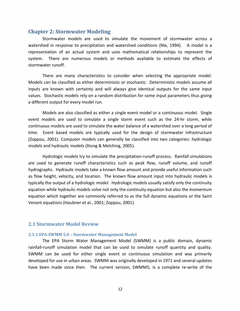
Chapter 2: Stormwater Modeling Stormwater models are used to simulate the movement of stormwater across a

watershed in response to precipitation and watershed conditions (Nix, 1994). A model is a

representation of an actual system and uses mathematical relationships to represent the

system. There are numerous models or methods available to estimate the effects of

stormwater runoff.

There are many characteristics to consider when selecting the appropriate model.

Models can be classified as either deterministic or stochastic. Deterministic models assume all

inputs are known with certainty and will always give identical outputs for the same input

values. Stochastic models rely on a random distribution for some input parameters thus giving

a different output for every model run.

Models are also classified as either a single event model or a continuous model. Single

event models are used to simulate a single storm event such as the 24-hr storm, while

continuous models are used to simulate the water balance of a watershed over a long period of

time. Event based models are typically used for the design of stormwater infrastructure

(Zoppou, 2001). Computer models can generally be classified into two categories: hydrologic

models and hydraulic models (Xiong & Melching, 2005).

Hydrologic models try to simulate the precipitation-runoff process. Rainfall simulations

are used to generate runoff characteristics such as peak flow, runoff volume, and runoff

hydrographs. Hydraulic models take a known flow amount and provide useful information such

as flow height, velocity, and location. The known flow amount input into hydraulic models is

typically the output of a hydrologic model. Hydrologic models usually satisfy only the continuity

equation while hydraulic models solve not only the continuity equation but also the momentum

equation which together are commonly referred to as the full dynamic equations or the Saint

Venant equations (Haubner et al., 2001; Zoppou, 2001).

2.1 Stormwater Model Review

2.1.1 EPA-SWMM 5.0 – Stormwater Management Model

The EPA Storm Water Management Model (SWMM) is a public domain, dynamic

rainfall-runoff simulation model that can be used to simulate runoff quantity and quality.

SWMM can be used for either single event or continuous simulation and was primarily

developed for use in urban areas. SWMM was originally developed in 1971 and several updates

have been made since then. The current version, SWMM5, is a complete re-write of the

13

previous versions and includes a graphical user interface which was absent in previous releases

(Rossman, 2009).

SWMM is considered to be primarily a hydraulic model although it also includes both

hydrologic and water quality components (Haubner et al., 2001). The runoff (hydrologic)

component of SWMM is computed based on the defined subcatchment areas that receive

precipitation and produce runoff and pollutant loads. The routing component routes the

generated runoff through a defined routing network which can be pipe systems, channels,

storage devices, pumps, and regulators. SWMM tracks the quantity and quality of runoff

produced and the flow rate, flow depth, and quality of the water in the routing network during

a simulation period comprised of multiple time steps (Gironas et al., 2009).

Subcatchment objects represent a land area that receives and collects precipitation and

allows infiltration and drainage to a common outlet node. The principal input parameters for

subcatchments are: Infiltration method, assigned rain gage, outlet node, assigned landuses,

surface area, imperviousness, slope, characteristic width of overland flow path, Manning’s n for

overland flow path on pervious and impervious areas, depression storage in both pervious and

impervious areas, and the percent of impervious areas with no depression storage (Rossman,

2009). Infiltration can be modeled using the Horton Method, the Green-Ampt Method, or the

SCS Curve Number method.

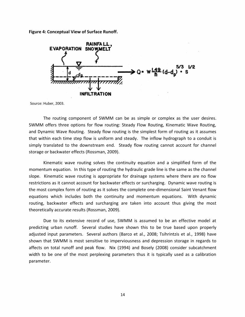
SWMM generates surface runoff and pollutant loads based on defined subcatchment

properties. SWMM uses nonlinear reservoir routing to simulate the surface runoff. Each

subcatchment is treated as a nonlinear reservoir and the continuity equation is coupled with

Manning’s equation for prediction of the outflow based on rainfall excess and surface

characteristics as shown in Figure 4 (Huber, 2003). Nonlinear reservoir routing is based on a

hypothesized relationship between outflow and water storage. In contrast other models use

the kinematic wave theory, which is based on the approximations of the real physical rainfall-

runoff process, to simulate surface runoff. However, Xiong (2005) concluded that the nonlinear

reservoir routing method would provide acceptable results for storms with durations longer

than the watershed time of concentration.

14

Figure 4: Conceptual View of Surface Runoff.

The routing component of SWMM can be as simple or complex as the user desires.

SWMM offers three options for flow routing: Steady Flow Routing, Kinematic Wave Routing,

and Dynamic Wave Routing. Steady flow routing is the simplest form of routing as it assumes

that within each time step flow is uniform and steady. The inflow hydrograph to a conduit is

simply translated to the downstream end. Steady flow routing cannot account for channel

storage or backwater effects (Rossman, 2009).

Kinematic wave routing solves the continuity equation and a simplified form of the

momentum equation. In this type of routing the hydraulic grade line is the same as the channel

slope. Kinematic wave routing is appropriate for drainage systems where there are no flow

restrictions as it cannot account for backwater effects or surcharging. Dynamic wave routing is

the most complex form of routing as it solves the complete one-dimensional Saint Venant flow

equations which includes both the continuity and momentum equations. With dynamic

routing, backwater effects and surcharging are taken into account thus giving the most

theoretically accurate results (Rossman, 2009).

Due to its extensive record of use, SWMM is assumed to be an effective model at

predicting urban runoff. Several studies have shown this to be true based upon properly

adjusted input parameters. Several authors (Barco et al., 2008; Tsihrintzis et al., 1998) have

shown that SWMM is most sensitive to imperviousness and depression storage in regards to

affects on total runoff and peak flow. Nix (1994) and Bosely (2008) consider subcatchment

width to be one of the most perplexing parameters thus it is typically used as a calibration

parameter.

Source: Huber, 2003.

15

2.1.2 PondPack

PondPack is a proprietary detention pond design and urban hydrology modeling

program owned by Bentley-Haestad Methods. PondPack can be used to analyze pre- and post-

developed watershed conditions and pond sizes, compute outlet rating curves, compute

interconnected pond routing, and compute hydrographs for multiple events (Bentley, 2009a).

PondPack offers many options in regards to simulating rainfall. It can be used to model any

duration or distribution for synthetic or real storm events (Haubner et al., 2001). PondPack also

offers several peak discharge and hydrograph computation methods including the rational

method, SCS method, and the Santa Barbara Unit Hydrograph method.

PondPack can be considered a hydrologic model with limited but useful hydraulic

features (Haubner et al., 2001). Unlike EPA SWMM, PondPack calculates the effective

precipitation and uses a unit hydrograph to generate the runoff hydrograph. Infiltration losses

can be modeled by using the SCS Curve Number method, Green and Ampt method, Horton

method, or the user can assume a constant loss. PondPack also has options for depression

storage.

PondPack generates surface runoff based on the defined subcatchment properties.

These include the subcatchment area and any properties associated with the selected

infiltration method. These properties will define the peak flow using either the rational or SCS

Peak Discharge method. A time of concentration must also be approximated in order to

generate a runoff hydrograph. PondPack offers 13 different methods for computing time of

concentration including user defined, TR-55, and others. The peak flow and time of

concentration associated with a unit hydrograph will result in a runoff hydrograph for the

defined subcatchment (Bentley, 2009a).

PondPack offers three different reach routing methodologies: Muskingum, Modified

Puls, and Translation. The Muskingum and Modified Puls methods take storage effects into

account as they are derived from a form of the continuity equation. Translation routing

provides no direct routing transformations of the hydrographs; it simply performs a time-shift

from the inflow to the outflow. PondPack offers no dynamic solution so if a reverse flow

situation arises, PondPack will not account for this thus making the model invalid for any

backwatering effects (Bentley, 2009a).

PondPack was designed to simulate urban hydrology and detention pond design. The

associated hydraulic features give PondPack the ability to model minor systems (Haubner et al.,

2001) but the complexity and accuracy of the model based on hydrologic/hydraulic routing has

been found to be inadequate as compared to other stormwater models (Borah et al., 2008).

16

2.1.3 CivilStorm

CivilStorm is a proprietary fully dynamic, mulit-platform, hydraulic modeling software

developed for the analysis of complex stormwater systems and is owned by Bentley-Haestad

Methods. CivilStorm can be used for storm sewer analysis, inlet analysis, pond analysis, culvert

analysis, open channel analysis, and outlet structure analysis. CivilStorm also has a built in

hydrology component that can model wet weather flow runoff.

The hydrology component of CivilStorm is very much the same as PondPack. CivilStorm

calculates the effective precipitation and uses a unit hydrograph to generate the runoff

hydrograph. Losses such as infiltration can be modeled by using the SCS Curve Number

method, Green and Ampt method, Horton method, or the user can assume a constant loss.

Surface runoff and peak flow is generated based on defined subcatchment properties and the

time of concentration. The peak flow and time of concentration associated with a unit

hydrograph will result in a runoff hydrograph for the defined subcatchment (Bentley, 2009b).

The routing component of CivilStorm differs from PondPack in the fact that CivilStorm

only offers dynamic routing. This routing method solves the complete St. Venant equations and

provides the most theoretically accurate results. In addition to the default dynamic engine

previously described, CivilStorm can also be set up to run the EPA-SWMM engine (Bentley,

2009b).

2.2 References

Barco, J., Wong, K.M., and Stenstrom, M.K. 2008. Automatic Calibration of the U.S. EPA SWMM

Model for a Large Urban Catchment. Journal of Hydrologic Engineering 134 (4), 466-474.

Bentley. 2009a. Bentley PondPack V8i User’s Guide. Bentley Systems, Exton, Pennsylvania.

Bentley. 2009b. Bentley CivilStorm V8i User’s Guide. Bentley Systems, Exton, Pennsylvania.

Borah, D.K., and Weist, J.H. 2008. Watershed Models for Stormwater Management: A Review

for Better Selection and Application. Proc. of World Environmental and Water Resources

Congress 2008, May 12-16 2008, Honolulu, Hawaii.

Bosely, E.K. 2008. Hydrologic Evaluation of Low Impact Development Using a Continuous,

Spatially-Distributed Model. Master’s Thesis, Virginia Polytechnic Institute and State

University.

Gironas, J., Rosner, L.A., and Davis, J. 2009. Storm Water Management Model Applications

Manual. EPA/600/R-09/007. U.S. Environmental Protection Agency, National Risk

Management Research Laboratory, Cincinnati, Ohio.

17

Haubner, S., Reese, A., Brown, T., Claytor, R., and Debo, T. 2001. Georgia Stormwater

Management Manual Volume 2: Technical Handbook. Georgia Department of Natural

Resources-Environmental Protection Division, Atlanta, Georgia.

Huber, W.C. 2003. Hydrologic Modeling Processes of the EPA Storm Water Management Model

(SWMM). Proc. of World Water & Environmental Resources Congress 2003, June 23-26

2003, Philadelphia, Pennsylvania.

Nix, S.J. 1994. Urban Stormwater Modeling and Simulation. Lewis Publishers, Baco Raton.

Rossman, L. 2009. Storm Water Management Model User’s Manual Version 5.0. EPA/600/R-

05/040, U.S. Environmental Protection Agency, National Risk Management Research

Laboratory, Cincinnati, Ohio.

Tsihrintzis, V.A., and Hamid, R. 1998. Runoff Quality Prediction from Small Urban Catchments

Using SWMM. Hydrological Processes 12 (2), 311-329.

Xiong, Y., and Melching, C.S. 2005. Comparison of Kinematic-Wave and Nonlinear Reservoir

Routing of Urban Watershed Runoff. Journal of Hydrologic Engineering 10 (1), 39-49.

Zoppou, C. 2001. Review of Urban Stormwater Models. Environmental Modeling and Software

16, 195-231.

18

Chapter 3: LID in Arkansas: The Determinants

“Low Impact Development (LID) is an approach to land development that uses various

land planning and design practices and technologies to simultaneously conserve and protect

natural resource systems and reduce infrastructure costs “(HUD, 2003). This document

pertains to the use of LID as an alternative approach to stormwater management. The overall

goal of LID is to control stormwater at the source by creating a hydrological functional

landscape that mimics the predevelopment or natural hydrology of a given area. This is

achieved through a variety of mechanisms such as infiltration, ponding, interception, and

evapotranspiration using Best Management Practices (Coffman et al, 1999).

Since the use or effectiveness of LID depends greatly upon the local climate, geology,

and hydrology of a site, it is important know where to find the data. This document

summarizes Arkansas data for the key determinants and variables that are used in LID design

and also provides resources for obtaining the data. It is important to note however, that the

figures, tables, data, etc., included are for illustrative purposes only and should not be used for

design. If possible, design should be based on site specific information gathered by field

investigation or other local data sources.

3.1 Climate

The majority of the state’s climate can be considered humid sub-tropical; however the

northern part of the state can be classified as having a humid continental climate. Arkansas has

four distinct seasons and they can all range from fairly mild to extreme. The topography of

Arkansas as well as its close proximity to the plains to the west and the Gulf of Mexico to the

south plays a crucial role in Arkansas’s climate and weather.

3.1.1 Rainfall

A common goal in applying LID is to keep as much stormwater on site as possible. That

is why it is important to recognize rainfall patterns for particular areas. The average annual

rainfall in Arkansas ranges from less than 46 inches to more than 64 inches per year (Figure 5).

Annual rainfall varies from the drier North to the wetter south with the exception of the Boston

and Ouachita Mountains. These mountain ranges have higher annual precipitation values than

their surrounding areas.

19

Figure 5: Average Annual Precipitation for Arkansas from 1970-2000.

Typically in engineering design, designers are concerned with design storm rainfall

depth. These depths are used to calculate stormwater runoff and to size structural BMPs and

other stormwater infrastructure. Table 2 shows design storm depths for different areas of the

state. These depths are estimated from rainfall maps found in Technical Paper No. 40. TP 40 is

a rainfall atlas of the United States for durations from 30 minutes to 24 hours and return

periods from 1 to 100 years. Certain runoff equations require the 24-hr duration so that is what

is shown in Table 2. Some cities, such as Fayetteville and Jonesboro, specify design storm

values in their stormwater and/or drainage manual.

When we talk about design storms, we are really discussing the frequency of that

event. Storm frequency is based on the statistical probability of a storm occurring in a given

Source: NRCS National Cartography and Geospatial Center

20

year. For example, a 10 year storm has a 10% chance of occurring in any single year while a 100

year storm has a 1% chance to occur in any single year. However, it is important to remember

that these storm events occur randomly and there is a possibility that the 100 year event can

occur in two consecutive years or it could not occur at all in a 500 year period.

Table 2: Rainfall Event Totals of 24-hr duration in Arkansas.

Regions of Arkansas 1 year Storm

(in)

10 year Storm

(in)

25 year Storm

(in)

50 year Storm

(in)

100 year Storm

(in)

Northwest Arkansas (Fayetteville) 4.08 6 6.96 7.92 8.64

Northeast Arkansas (Jonesboro) 3.88 5.58 6.35 6.99 7.7

Southwest Arkansas 4.45 6.8 7.9 8.85 9.9

Southeast Arkansas 4.35 6.5 7.2 8 9

Resource:

1. Technical Paper 40 maps for Arkansas can be found online at:

http://www.nws.noaa.gov/oh/hdsc/currentpf.htm

3.2 Earth Resources

3.2.1 Geology/Soils

Since many LID BMPs rely heavily on the infiltration of rainwater and stormwater runoff,

it is important to consider and understand the soil properties and underlying geology (Figure 6)

that control the balance between infiltration, runoff, and groundwater elevations. Soil type

and texture class determine the rate of infiltration, the amount of water stored in soil pores,

and the relative effort required by evaporation or plant roots to draw water back up against

gravity.

Other important considerations for BMP design are depth to groundwater and depth to

bedrock. In fact, all these landscape properties can constrain the design of infiltration BMPs.

For example, karst formations are present in Northern Arkansas and must be considered before

designing LID structures that rely on infiltration. Karst formations are formed by the dissolving

action of water on carbonate bedrock such as limestone or dolomite. When infiltration into

these karst formations is increased, the dissolution of the bedrock is accelerated which can lead

to subsurface voids and sinkholes. Karst formations are also characterized by complex

Source: TP No. 40; City of Fayetteville, AR Drainage Manual; City of Jonesboro, AR Stormwater Drainage

Design Manual

21

underground drainage systems. This poses potential hazards to groundwater if infiltration

BMPs that are receiving water with high pollutant concentrations infiltrate into these

formations.

Figure 6: Arkansas Geologic Features Map

Source: United States Geological Survey, 2000, The Geologic map of Arkansas, Digital Version: U.S. Geological

Survey.; http://cpg.cr.usgs.gov/pub/other-maps.html

22

Water1%

A0%

B32%

C38%

D29%

Figure 7: Distribution of Hydrologic Soil

Groups in Arkansas

Successfully implementing LID requires balancing and understanding all the variables

that affect site hydrology. Soils are a key variable that affects hydrology. A soil’s infiltration

capacity should be understood in relation to the soil’s ability to filter or remove pollutants

before reaching groundwater. For example, clays have extremely low infiltration rates but

have the highest capacity for pollutant removal while sand has high infiltration rates but a very

low capacity for pollutant removal.

3.2.2 Hydrologic Soil Groups

All soil series are assigned to a Hydrologic Soil Group (HSG). These HSGs, A-D, are based

on a range of permeability, physical properties such as texture and depth to bedrock, and the

seasonal high water table (Table 3). All soils are permeable and drain to some degree unless

they are saturated by hydrologic conditions, such as hydric soils in a wetland. In regards to

infiltration potential, class A soils have high infiltration rates and are very well drained.

However, class D soils have little or no infiltration potential especially during rainfall and

produce much greater surface runoff.

Table 3: Hydrologic Soil Groups

Soil Group Soil Type Drainage Capacity

A Sand, loamy sand, sandy loam Very well drained and highly

permeable

B Silt loam, loam Good

C Sandy clay loam Fair

D Clay loam, sandy clay, silty clay, clay Poorly drained

The majority of soils in Arkansas are

classified in HSG C or D according to State

Soil Geographic Database (STATSGO) data for

Arkansas. Figures 7 and 8 show the

distribution of soils in Arkansas. County soil

surveys should be used as a preliminary

source for soil characterization. However,

site specific soil testing should be done

before final design and implementation of

23

LID projects in order to confirm soil characteristics such as infiltration rate.

Figure 8: Hydrologic Soil Groups of Arkansas

Source: United Sates Department of Agriculture, Natural Resources Conservation Service. 2005. Digital General Soil

Map of U.S.; http://SoilDataMart.nrcs.usda.gov

Resource:

1. Soil survey data are available online from NRCS Soil Surveys at:

http://websoilsurvey.nrcs.usda.gov/app/

24

3.2.3 Biotic Resources

The biotic resources of Arkansas span a vast array of flora and fauna. These organisms

impact the effectiveness of stormwater management programs and are impacted by the

programs set in place. For example, microbial processes occurring in the soil break down

pollutants while plant communities intercept rainfall and promote infiltration as well as

providing nutrient and pollutant uptake. However, these functions cannot happen if their

habitats and landscapes are not preserved. Everything is connected. Each plant, animal, and

microorganism is interdependent on one another within the ecosystem and is greatly impacted

by the abiotic environment.

LID involves capitalizing on the unique opportunities afforded by natural systems.

Preserving natural landscapes and habitats increases biological diversity and helps conserve

natural resources such as water, vegetation, and soil. This should be a priority in LID design.

However, if preservation is not possible or if more diversity is desired, use designs that mimic

natural systems as this leads to more biological diversity and increased biological diversity leads

to increased stormwater treatment capacity. Figure 9 provides a graphical summary of current

land use/land cover throughout Arkansas.

25

Figure 9: Land Use/Land Cover for Arkansas Fall 2006

When applying LID to a site, the plant community should be inventoried and compared

to the ecoregion. (Ecoregions are simply areas of general similarity in ecosystems and in the

type, quality, and quantity of environmental resources. The ecoregions of Arkansas are shown

in Figure 10.) It is important that designs for LID BMPs include native plants and exclude the

exotic and invasive species that have been introduced into wild flora. Native plants offer many

more benefits than non-natives while still providing essential functions such as stormwater

nutrient removal and increased infiltration rates. Native plant species often require less

maintenance once established because they are acclimated to local climate and conditions

therefore being drought and disease tolerant. Native plants help to create a self-sustaining

natural habitat. Plant selection criteria should be based on an ecoregion (Fig. 10) to ensure that

plants can survive and flourish in the specific climatic and environmental conditions of the site.

Source: Center for Advanced Spatial Technologies. 2007. Land Use Land Cover Fall 2006;

http://www.geostor.arkansas.gov

26

Figure 10: Eco-Regions of Arkansas

Resources:

1. Information on landscaping and plant selection from the Univeristy of Arkansas

Cooperative Extension Service can be found online at:

http://www.arhomeandgarden.org/landscaping.htm

2. Information about ecoregions of Arkansas can be found online at:

http://www.epa.gov/wed/pages/ecoregions/ar_eco.htm

http://www.wildlifearkansas.com/ecoregions.html

Source: USEPA. 2004. Ecoregions Level III and IV 2004; http://www.geostor.arkansas.gov

27

3.3 Sensitive Areas

When implementing LID in Arkansas, it is important to understand the connection of the

site to sensitive areas such as wetlands, high quality waters, wellhead protection areas, and

impaired waterways. These areas could have potential constraints that may require changing

the LID design in order to protect these resources.

3.3.1 Wetlands

In Arkansas, only 2.8 million of the original 9.8 million acres of wetlands remain which

represents 8% of the surface area of the state (Dahl, 1990). Wetlands can be found in most

parts of the state but the majority are found within the floodplains of the Mississippi River and

its major tributaries.

Wetlands are very diverse and important resources. They also provide services such as

water storage, water quality improvement, and habitat for many diverse species of both plants

and animals. Because of their importance, most wetlands should not be subjected to significant

hydrologic or water quality alterations. One BMP in LID design is a constructed wetland. These

constructed wetlands can be a restoration of a historically lost wetland or construction of a new

wetland where they have never existed before. Constructed wetlands are true treatment

systems. They can receive stormwater runoff, allow sediment to settle, and most importantly

they can biologically remove nutrients and other pollutants from stormwater.

Resource:

1. Detailed descriptionof wetland types and wetland protection plans for Arkansas can be

found at http://www.mawpt.org/

3.3.2 Wellhead Protection Areas/Public Water Supply

Wellhead protection areas and public water supply areas are considered sensitive areas

because many individuals rely on groundwater as their source of drinking water. LID practices,

specifically infiltration, must be assessed carefully in these areas. Normally, infiltration BMPs

will provide a high degree of filtering of stormwater runoff if correctly sized, but certain

geologic features such as high water table in a public water supply area with high infiltration

soils or karst formations may require further analysis.

28

Resource:

1. Source water protection information can be found at

http://www.healthyarkansas.com/eng/swp/swp.htm

3.3.3 Sensitive Waters

Arkansas has many waterways that are designated as either high quality or outstanding

resource waters by the Arkansas Department of Environmental Quality (ADEQ). These include

extraordinary resource waters, ecologically sensitive waters, and natural and scenic waterways.

Arkansas also has waterways that are currently designated as impaired and may need special

consideration as well.

These outstanding resource waters must be protected. Extraordinary resource waters

are identified by a combination of the chemical, physical, and biological characterisitics of a

waterbody and its watershed. An ecologically sensitive waterbody is a waterbody that is known

to provide habitat to threatened, endangered or endemic species of aquaitc of semi-aquatic

life. A natural and scenic waterway is one which has been legislatively adopted into a state or

federal system (See Figure 11). Normally LID would be the development practice most

consistent with ensuring water quality, however in some instances, such as highly permeable

soils, special considerations for treatment of runoff should be investigated.

Resource:

1. More information about ADEQs designations of waterways and the water quality

standards associated with these designations can be found at

http://www.adeq.state.ar.us/regs/files/reg02_final_071125.pdf

29

Figure 11: Designated Natural and Scenic Waterways of Arkansas

Source: Arkansas Department of Environmental Quality. 2008. Natural and Scenic Waterways;

http://www.geostor.arkansas.gov

30

3.4 References

Coffman, L.S., R. Goo, R. Frederick. 1999. Low-Impact Development: An Innovative Approach to

Stormwater Management. In Proc. 29th Annual Water Resources Planning and Management

Conference, ASCE, Reston, Va., 118

Dahl, T. E. 1990. Wetland Losses in the United States 1780’s to 1980’s. U.S. Department of the

Interior, Fish and Wildlife Service. Washington, D.C. 13pp.

Southeast Michigan Council of Governments. 2008. Low Impact Development Manual for

Michigan: A Design Guide for Implementers and Reviewers. Southeast Michigan Council of

Governments Information Center.

U.S. Department of Housing and Urban Development (HUD). 2003. The Practice of Low Impact

Development (H-21314CA). Washington, DC: Government Printing Office.

31

Chapter 4: LID Best Management Practices

4.1 Underground Detention

Underground detention systems are structural Best Management Practices that collect,

detain and slowly release stormwater back into the stormwater system, or into the ground,

depending on the design and the location. Underground detention is useful in areas where

available space is minimal. They are typically installed beneath streets, buildings, parks, and

parking lots in order to maximize property use. Underground detention tanks are intended to

be used as an integral part of a larger system of flow attenuation facilities. In the site plan, they

are placed downstream from catchment infrastructure.

Figure 12: Underground detention system.

Source: UA CDC. http://uacdc.uark.edu

32

This type of stormwater management technology reduces runoff volume by collecting

the runoff prior to it reaching nearby stormwater drainage systems or local streams.

Depending on the location and design, underground detention tanks address the need to

reduce site discharge, as well as offer the potential for infiltration, if designed to do so. This

type of LID technology also slows runoff velocity, therefore allowing sediment to drop out and

improve water quality. Underground detention systems tend to be easy to maintain and

relatively low in cost.

Resources:

Low Impact Development Manual for Michigan. 2008. pp. 122, 147, 343.

Urban Design Tools – Low Impact Development. 2007.

4.2 Infiltration Basin

Infiltration basins are shallow, impounded areas with highly permeable soils, designed

to temporarily detain and infiltrate stormwater runoff. These LID stormwater attenuation

facilities are intended to improve water quality by filtering runoff through the soil and

subsequently recharging the groundwater supply. In addition to water filtration, infiltration

basins use plants that trap sediment and take up nutrients within the stormwater runoff.

Infiltrations require highly permeable soils. As with other LID technologies, infiltration basins

are intended to act as part of a more complex system of attenuation facilities. The best use of

an infiltration basin within a site plan is downstream from other flow attenuation and filtration

facilities within a catchment, as well as upstream from overflow/outflow facilities within the

stormwater drainage system.

Infiltration basins provide a way to reduce runoff volume, as well as to reduce the peak

rate runoff. This technology, in turn, facilitates groundwater recharge and improves overall

water quality. Wildlife habitat is also a benefit of infiltration basins when native plant species

are used and these systems can add aesthetic value to a property. Infiltration basins, for

example, can be installed as play fields in parks; therefore providing multiple uses for a single

piece of property. Infiltration basins require little maintenance and performance may improve

over time as vegetation becomes more mature.

33

Figure 13: Infiltration basin system.

Resources:

Low Impact Development Manual for Michigan. 2008. pp 193-219

Stormwater Management Handbook. 2009. Pp. 30-32.

4.3 Rainwater Harvesting

Rainwater harvesting through the use of cisterns or rain barrels uses storage as a

method of managing stormwater. Cisterns are generally larger than rain barrels and used for

water supply, rather than irrigation for landscaping. Cisterns and rain barrels can be connected

to provide increased storage. Rainwater harvesting reduces runoff volume thus reducing peak

discharge. These types of systems are optimal for residential or commercial use. The

management of stormwater through the use of rainwater harvesting is one step in an

integrated stormwater management plan for a site. Rainwater harvesting systems are located

upstream in a catchment. Rain barrels or cisterns collect rainwater near its source (rooftops)

and store it for future use.


34

Rainwater harvesting provides opportunities for water reuse in homes or buildings or

for irrigation. This type of BMP can also provide aesthetic beauty in the architectural design of

a home or business. As a result of a reduction in runoff volume, rainwater harvesting reduces

water quality impairment by reducing the potential of surface erosion caused by stormwater

runoff for high frequency storm events. Rain barrels and cisterns are an optimal tool for use in

retrofit projects, or in locations with minimal space availability. Maintenance needs are

considered to be moderate as compared to other LID technologies however water must be

used periodically between rain events to maximize storage capacity and minimize runoff.



Figure 14: Cistern system.

Figure 15: Rain barrel system.

35

Resources:

Low Impact Development Manual for Michigan. 2008. Pp. 147-156.

Low Impact Development Design Strategies – An Integrated Design Approach. 1999. 4.18-4.19.

Low Impact Development Technical Guidance Manual for Puget Sound. 2005. Pp. 133-140.

United States Department of Housing and Urban Development. 2003. Pp. 43-44.


4.4 Vegetated Filter Strip

A filter strip is a vegetated area of land used to manage stormwater runoff by providing

flow attenuation. This type of LID technology uses vegetation to slow runoff velocity, thus

allowing suspended sediment and debris loads to drop out and accumulate in the filter strip

instead of in the stormwater drainage system or local stream. As a result of these processes,

filter strips decrease peak discharge and decrease water quality impairment through the

reduction of nutrients and sediment. Filter strips are often located next to roads so that

stormwater flows along the length of the strip, rather than by curb to a single outlet. The filter

strip LID facility is upstream of other treatment systems and is therefore referred to as a pre-

treatment device. As with other LID tools, it is intended to be part of a site’s integrated

stormwater management plan. Filter strips are intended to protect other filtration systems

from becoming clogged with sediment or other debris. This requires that there be optimal

space for settling of sediment or debris loads. Pre-treatment systems, such as a filter strip,

require regular inspection and maintenance to ensure that the filter strip has not become

clogged with sediment and/or debris.

Figure 16: Vegetated filter strip system.


36

Resources:

Low Impact Development Design Strategies – An Integrated Design Approach. 1999. Pp. 4.12-

4.14.



4.5 Pervious Pavement

Pervious pavement is an infiltration technique that can combine stormwater infiltration,

storage, and structural pavement. Paving consists of a permeable surface which may include a

subsurface base made of course aggregate. It provides pre-treatment by removing sediment

and other pollutants. This is a useful stormwater management tool that reduces stormwater

volume and encourages groundwater infiltration. There are multiple types of pervious paving

designs, including manufactured pavers, porous asphalt, porous concrete, and gravel. Pervious

paving reduces the amount of impervious surface area for a site. Pervious paving is upstream

in a site catchment and treats water at the source. When rain water falls on pervious pavers it

is allowed to soak through the porous surface and into amended and highly permeable soil

underneath. In some designs, under the pervious pavement is a system of layers composed of

soil, gravel and sand to increase storage and maximize infiltration.

This type of LID design provides reductions in peak discharge from a site, as well as

improved water quality benefits. Pervious pavers allow for groundwater recharge. Pervious

pavers provide a means of reducing standing water on roads, driveways and parking lots.

Finally, reducing imperviousness through the use of pervious pavers increases time of

concentration, and therefore reduces damage to stormwater drainage systems and local

streams. Pervious pavers require inspections and maintenance in order to prevent clogging by

sediment and debris. They require regular sweeping and/or street vacuuming to maintain the

ability of water to infiltrate.

37

Figure 17: Different pervious pavement systems.

Source : UA CDC. http://uacdc.uark.edu

Resources:

Start at the Source. 1999. Pp. 46-53




38

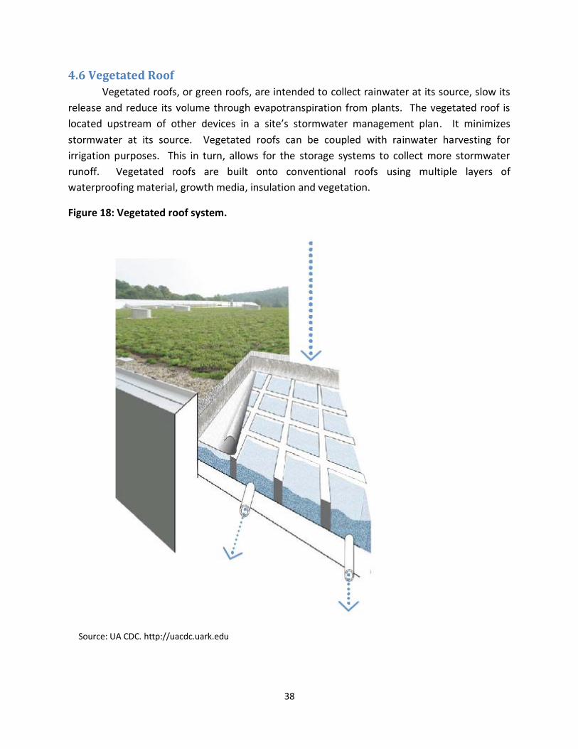
4.6 Vegetated Roof

Vegetated roofs, or green roofs, are intended to collect rainwater at its source, slow its

release and reduce its volume through evapotranspiration from plants. The vegetated roof is

located upstream of other devices in a site’s stormwater management plan. It minimizes

stormwater at its source. Vegetated roofs can be coupled with rainwater harvesting for

irrigation purposes. This in turn, allows for the storage systems to collect more stormwater

runoff. Vegetated roofs are built onto conventional roofs using multiple layers of

waterproofing material, growth media, insulation and vegetation.

Figure 18: Vegetated roof system.


39

Vegetated roofs reduce stormwater runoff but also can provide home temperature

regulation through additional thermal insulation, reducing the need for heating and cooling. In

addition, they provide an aesthetic value that has the potential to increase property value. As a

result of their ability to reduce runoff and peak discharge, vegetated roofs contribute to

increasing the water quality of streams through the reduction of sediment and nutrient loads.

There are varying maintenance needs for vegetative roofs as result of the plants and the growth

media. There are three types of vegetated roofs; intensive, semi-intensive and extensive. Each

type requires varying levels of maintenance. The Intensive-style vegetative roofs require the

most maintenance and all types may require structural inspection to ensure that the building

can withstand the increased.

Resources:


4.22.




EPA Green Infrastructure

4.7 Tree Box Filters

Tree box filters are within a broader category often referred to as Planters Boxes. These

are devices that are installed beneath trees, shrubs or flowers and located within streets,

sidewalks and building walls. Sidewalk planters, such as tree box filters, are used as part of a

pre-treatment system which filters water prior to entering the stormwater or sewer system.

They are designed to provide flow attenuation, as well as water quality treatment through

filtration. They require curb cuts to allow flow. Planter boxes along building walls slow and

reduce runoff from a building’s impervious footprint. Planter boxes are located on the

upstream end of the treatment train. Tree box filters work as part of an integrated

bioretention/rain garden stormwater management plan that provides water quality

improvement.

Planter boxes use layers of soil, mulch and an underdrain system to slow and filter

stormwater runoff. This type of LID technology can provide services such as aesthetic beauty,

increased property values, groundwater infiltration, and decreased runoff volume. Allowing

stormwater to runoff into planters can help irrigate the trees or shrubs reducing the need for

municipal irrigation. Using planter boxes improve the wildlife habitat availability in urban areas,

while they reduce pollutant loads in stormwater runoff. As a result, this type of design can be

incorporated in urban retrofits with the added benefit of reducing the urban heat island effect.

40

As with other low impact development filtration devices, planter boxes require occasional

inspection to remove large debris and/or trash.

Figure 19: Tree box filter system.

Resources:

Low Impact Development Manual for Michigan. 2008. Pp. 257-266

Urban Design Tools – Low Impact Development. 2007.

4.8 Infiltration Trench

Infiltration trenches are subsurface linear features lined with geotextile fabric and a

perforated pipe. They slow, filter and detain stormwater runoff through layers of sand and


41

gravel. Infiltration trenches are used to control runoff volume through infiltration. These

devices promote groundwater recharge and water filtration, thus reducing peak discharge and

improving water quality. Water quality is improved because of the reduction in sediment and

nutrient loads to local streams and drainage systems. This LID technology is an intermediate

stormwater management system located upstream from major storage and/or treatment

facilities, but downstream from smaller filtration devices. The maximum catchment area for

infiltration trenches is 2 acres; therefore it is necessary to incorporate other LID features into

the stormwater management plan along with infiltration trenches.

Figure 20: Infiltration trench system.

An infiltration trench can be constructed in a more confined area than an infiltration

basin, making it a more versatile tool in urban stormwater design. Infiltration trenches require

less maintenance if upstream pre-treatment filters are installed, such as filter strips or devices.


42

This reduces clogging within the trench. Occasional inspection is recommended to remove

large debris and/or trash.

Resources:


4.12, 4.20-4.21.



4.9 Constructed Wetland

Constructed wetlands can be established in historically drained wetland areas or low

areas located within a site. Wetland areas receive stormwater runoff, reduce the velocity and

allow sediment to settle out. Wetlands biologically and chemically treat nutrients and other

pollutants in stormwater during retention. In addition, wetlands allow for evapotranspiration

which can reduce runoff volume. These systems are planted with native vegetation which

improves nutrient uptake therefore improving water quality. Constructed wetlands are

located downstream in the treatment train from other infiltration and filter devices. As with

other infiltration systems, pre-treatment systems upstream from constructed wetlands help to

remove sediment that will fill and clog a wetland system. Constructed wetlands can be

incorporated into existing turf grass areas by diversifying the vegetation and therefore

increasing ecosystem services provided by that land use.

Figure 21: Constructed wetland system.


43

Constructed wetlands provide a wide spectrum of benefits in regard to stormwater

management. As a result of the diverse vegetation, these systems provide evapotranspiration,

nutrient uptake and assimilation, wildlife habitat and aesthetic beauty. In addition, constructed

wetlands reduce peak discharge to streams and municipal stormwater systems and may

contribute to groundwater recharge. Once a constructed wetland is established, it takes little

maintenance. In the first two years after establishment, there is more maintenance required in

order to establish vegetation and a maintenance plan is recommended. Some locations choose

to hold the wetland area in a conservation easement, thus ensuring the maintenance and

integrity of the wetland system.

Figure 22: Completed constructed wetland.


Resources:



4.10 Oversized Pipe

Oversized pipes are subsurface systems which are designed to attenuate flow and thus

reduce peak discharge. Water enters a large inflow pipe and leaves through a smaller outflow

pipe, thus restricting flow. The large volume of the pipe allows water to be detained, without

creating problematic backwater effects. This stormwater BMP can also address water quality by

44

slowing the water and allowing the sediment to settle out prior to leaving the outflow pipe.

The location of oversized piping can vary within the treatment train. This type of system can be

upstream from other LID facilities or downstream prior to entering the municipal stormwater

drainage system or local stream. Subsurface oversized pipes act like detention systems in that

they are designed to empty slowly in between runoff events. Oversized pipes can be used in

retrofit scenarios if the site is located upstream in the drainage basin. As with other subsurface

LID technologies, oversized pipes offer a stormwater management tool for sites with minimal

surface space available

Figure 23: Oversized pipe system.

Water quality improvements will be minimal; however oversized pipes will help reduce

sediment loads. The primary benefits come with the reduction in runoff velocity and peak flow

which reduces outflow erosion and stream bank erosion. Upstream pre-treatment filter

facilities are recommended to reduce the inflow of large debris into the oversized pipes. Due to


45

sediment settling, pipes may need to be cleaned out periodically. Other maintenance needs are

minimal and comparable to convention pipe inspection and maintenance needs.

Resource:

Model Stormwater Management Ordinance. 1993. Pp. 3.297-3.300

4.11 Dry Pond

Dry ponds, also known as detention ponds, are stormwater management elements

which detain stormwater and allow for the slow release of runoff to the stormwater system or

receiving waterbody. The primary purpose of dry ponds is to attenuate flow and therefore

reduce the peak discharge rate. Dry ponds are located downstream of other stormwater

treatment facilities and upstream from municipal stormwater management systems.

Figure 24: Completed dry pond system.


Detention ponds are designed to completely empty out between runoff events, and

therefore provide mainly runoff rate control as opposed to water quality control. The

reduction in peak discharge protects downstream stream systems from scouring and habitat

loss. They are most effective with paired with an integrated system of BMPs throughout the

catchment. Dry ponds require some maintenance for trash and sediment removal periodically.

In addition, vegetation within dry ponds requires periodic mowing.

46

Resource:


4.12 Wet Pond

A wet pond, also known as a wet pool or retention pond, is a constructed stormwater

pond that retains a permanent pool of water. Wet ponds provide water quality treatment and

detention. Wet ponds can remove pollutants not only through sedimentation but also through

biological uptake processes, whose removal of pollutants is proportionate to the length of time

runoff remains in the pond. Wet ponds do address peak discharge rates through detention, but

do not reduce total runoff volume. Groundwater infiltration from wet ponds is minimal, as

water stays in the pond and provides habitat for plants and other organisms. Wet ponds are

located downstream within a catchment system and are most effective when combined with

other flow attenuation and filtration BMPs. They can act in-line with other treatment systems

or off-line as standalone systems.

Figure 25: Wet pond system design.


Wet ponds provide aesthetic beauty and habitat while also providing water treatment

and reduced peak flows. Wet ponds can be used in many settings such as residential, industrial

or commercial. These systems are more difficult to establish in areas where space is limited.

They can provide attractive green space while also functioning as a stormwater management

tool used to reduce sediment and nutrient levels in runoff. Regular maintenance inspections

are needed to ensure proper drainage and vegetative health. Trash, debris, and sediment will

need to be removed periodically.

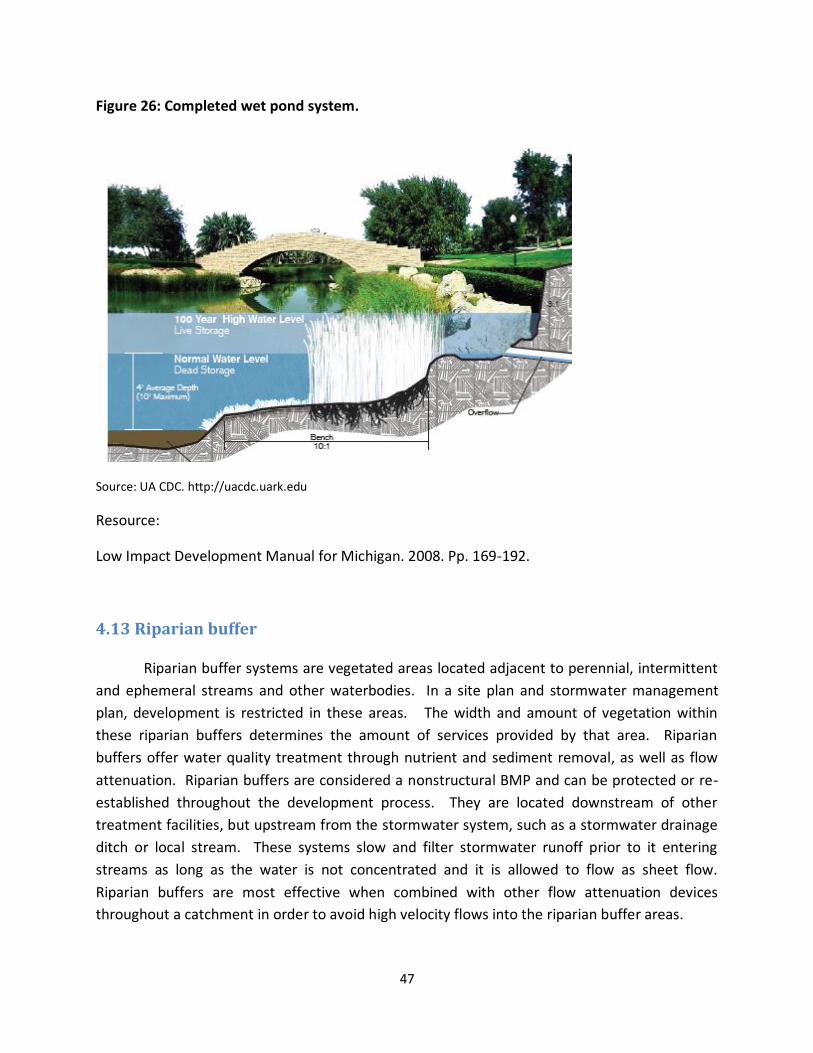
47

Figure 26: Completed wet pond system.


Resource:


4.13 Riparian buffer

Riparian buffer systems are vegetated areas located adjacent to perennial, intermittent

and ephemeral streams and other waterbodies. In a site plan and stormwater management

plan, development is restricted in these areas. The width and amount of vegetation within

these riparian buffers determines the amount of services provided by that area. Riparian

buffers offer water quality treatment through nutrient and sediment removal, as well as flow

attenuation. Riparian buffers are considered a nonstructural BMP and can be protected or re-

established throughout the development process. They are located downstream of other

treatment facilities, but upstream from the stormwater system, such as a stormwater drainage

ditch or local stream. These systems slow and filter stormwater runoff prior to it entering

streams as long as the water is not concentrated and it is allowed to flow as sheet flow.

Riparian buffers are most effective when combined with other flow attenuation devices

throughout a catchment in order to avoid high velocity flows into the riparian buffer areas.

48

Figure 27: Riparian buffer.

Riparian buffers offer many ecological services in addition to flow attenuation and water

quality treatment through vegetative filtering and uptake. Riparian zones provide temperature

management, infiltration and groundwater recharge in areas where the water table is below

bankfull levels. They provide wildlife habitat and aesthetic beauty. In addition vegetation can

stabilize streambanks. Some maintenance is required to manage the vegetation in areas where

riparian buffers are near residential and/or commercial development.

Resource:



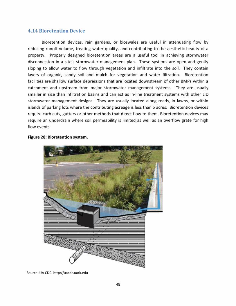
49

4.14 Bioretention Device

Bioretention devices, rain gardens, or bioswales are useful in attenuating flow by

reducing runoff volume, treating water quality, and contributing to the aesthetic beauty of a

property. Properly designed bioretention areas are a useful tool in achieving stormwater

disconnection in a site’s stormwater management plan. These systems are open and gently

sloping to allow water to flow through vegetation and infiltrate into the soil. They contain

layers of organic, sandy soil and mulch for vegetation and water filtration. Bioretention

facilities are shallow surface depressions that are located downstream of other BMPs within a

catchment and upstream from major stormwater management systems. They are usually

smaller in size than infiltration basins and can act as in-line treatment systems with other LID

stormwater management designs. They are usually located along roads, in lawns, or within

islands of parking lots where the contributing acreage is less than 5 acres. Bioretention devices

require curb cuts, gutters or other methods that direct flow to them. Bioretention devices may

require an underdrain where soil permeability is limited as well as an overflow grate for high

flow events

Figure 28: Bioretention system.


50

Bioretention areas provide groundwater recharge, water filtration, water temperature

maintenance, and wildlife habitat. Bioretention areas remove nutrients, as well as sediment.

They are versatile and provide a disconnected system of treatment sites within a stormwater

management plan and can be used to retrofit an existing development. These designs can be

implemented in all types of developments, but are more difficult in intensely urban areas

where surface space is limited. For the first 2 years, more maintenance is required in order to

establish vegetation. On-going inspections for sediment and trash accumulation are needed.

Resources:


4.10.




Stormwater Management Handbook. 2009. Pp. 22-25, 30-33.

4.15 Flow Control Devices

Flow control devices, such as flow splitters, are used as methods for reducing peak

discharge through the systematic placement of devices which attenuate concentrated flow.

These systems provide the most benefit to water and stream quality when combined with other

integrated LID facilities. Flow control devices are located upstream from infiltration facilities

and downstream from the source, such as a roof or a parking lot. These devices are placed in

areas of concentrated sheet flow or channel flow in order to attenuate the flow prior to

entering the stormwater management system.

Flow control devices slow down surface runoff, thus allowing large debris and sediment

to drop out of suspension. These devices are intended to improve the function of other LID

facilities by redirecting or slowing flows. Runoff velocity, peak discharge and sediment loads

are reduced as a result of using flow control devices. These systems require regular

maintenance and inspection to remove excess sediment, trash and debris.

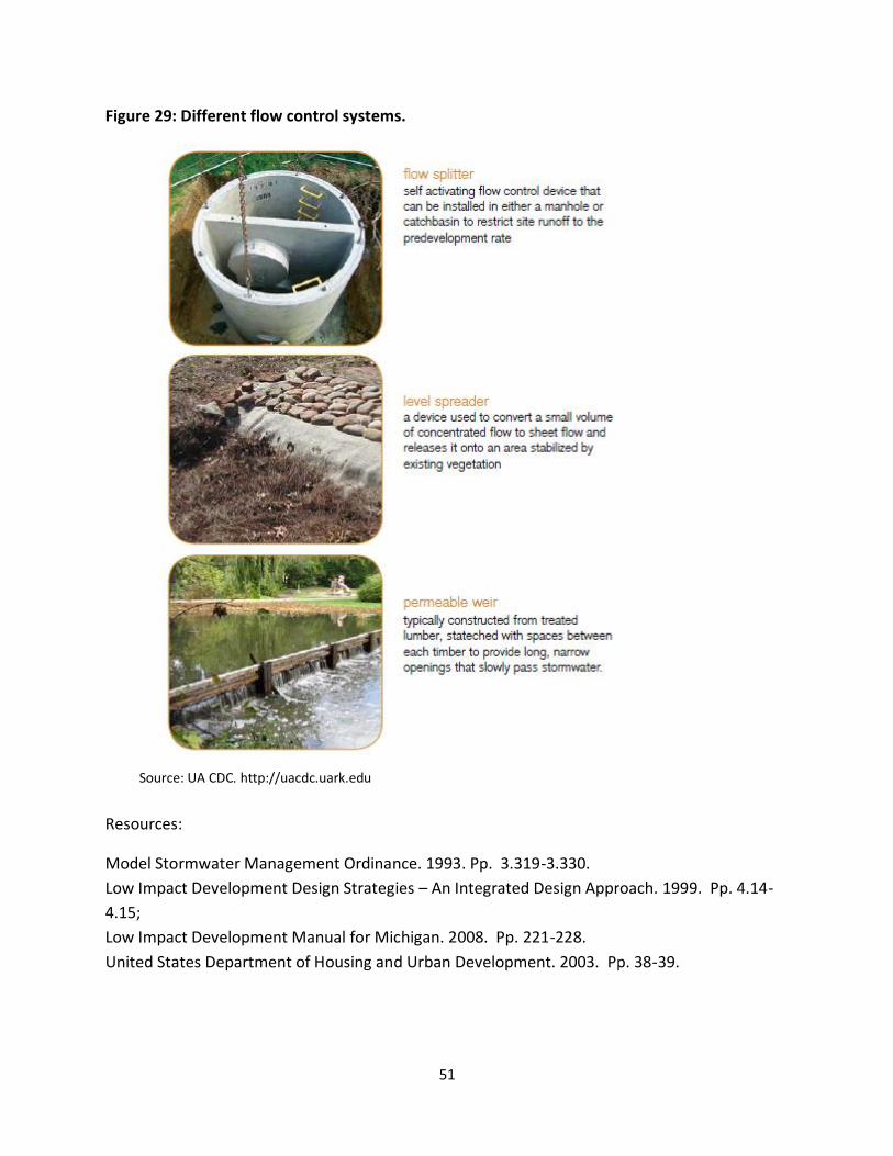
51

Figure 29: Different flow control systems.

Resources:

Model Stormwater Management Ordinance. 1993. Pp. 3.319-3.330.


4.15;




52

4.16 Wet Vault

Wet vaults are subterranean areas where stormwater runoff is collected and a

permanent pool is maintained. These systems do not empty in between runoff events. Wet

vaults contribute to stormwater flow attenuation, as well as some water quality treatment.

Wet vaults are located upstream from major stormwater management systems and

downstream from other LID treatment facilities within a catchment.

Figure 30: Wet vault system.

As a result of the permanent water retention, wet vaults are able to remove more

sediment than other subterranean storage devices which slowly drain completely. In a wet

vault, water slowly seeps out into other stormwater management facilities. This type of design

provides runoff volume control, reduced peak discharge, sediment control, as well as the

potential for water reuse. Minimal maintenance is required of these systems. Periodic

inspection of in-flow areas is needed to remove large debris, sediment and/or trash.

Resource:



53

4.17 Erosion Control Device

Erosion increases sedimentation and destabilizes stream banks, reducing habitat

function and water quality. Erosion control devices are used to prevent and control erosion

from stormwater in agriculture, land development and construction. Erosion control devices

such as erosion control blankets and silt fences hold sediment in place or limit the amount

reaching stormwater during runoff events. Slope stabilizers act hold stream banks or steep

slopes in place during high flow events. Non-structural management practices should also be

undertaken. These include measures such as cover cropping open soil, minimizing time

between clearing land and vegetation and beginning construction, or planning construction to

avoid rainy seasons where possible. These devices are located at or near the source. They are

intended to hold soil and sediment in place before it enters the stormwater system. These

devices are usually upstream from LID facilities and are therefore useful in preventing sediment

accumulation in infiltration basins and other LID facilities.

Figure 31: Different erosion

control devices.


54

Erosion control devices reduce loss of soil as a result of water erosion. They protect

water quality by limiting the amount of sediment that enters the runoff. In some cases, such as

properly installed silt fences, erosion control devices can also slow runoff velocity. These types

of designs are useful during the construction phase of a development because they are readily

installed and easily removed. Erosion controls require inspections and maintenance to ensure

that the devices are installed properly and have not become dislodged or too full of debris and

sediment.

Resources:


Low Impact Development Design Strategies – An Integrated Design Approach. 1999. Pp.5-7.

4.18 Vegetated Swale

Vegetated or dry swales provide water quality treatment, flow attenuation, and

infiltration into groundwater. Vegetated swales, convey water much as a concrete channel, but

flow over a vegetated and often sinuous channel which reduces flow velocity and leads to the

settling out of sediment and filtering of other pollutants. In addition, they can be designed with

check dams and underdrains to detain stormwater and increase infiltration. Dry swales are

good options in residential settings, as they help convey water away from houses and roads in a

controlled manner, discouraging standing water. Dry swales are often located in a drainage

easement at the back or side of a residential lot or along roadsides and parking lots in place of a

curb and gutter. Swales can be used as a pre-treatment mechanism upstream from other LID

facilities. They can also be located downstream from control devices, such as check dams, so

that concentrated flow does not cause erosion of the swale.

Dry swales are useful in all types of development applications including residential,

commercial, urban, and retrofit areas. They treat water quality thus improving stream habitat.

They reduce peak discharge and therefore protect stream bank integrity. Dry swales can also

provide aesthetic beauty to a site and provide wildlife habitat depending on the type of

vegetation used. Irrigation is necessary in periods of minimal rain. Early in establishment,

stabilization of seeds is necessary through the use of erosion control devices. Periodic

inspections of dry swales are needed in order to manage vegetation growth, and remove large

debris and/or trash. In addition, annual inspection should assess the slope of the dry swale, as

well as the infiltration rate.

55

Figure 32: Vegetated swale system.


Resources: Low Impact Development Design Strategies – An Integrated Design Approach. 1999. Pp. 4.16-4.18; Low Impact Development Manual for Michigan. 2008. Pp. 315-327. United States Department of Housing and Urban Development. 2003. Pp. 40-43. Stormwater Management Handbook. 2009. Pp. 22-25.

4.19 Sand Filters (Surface and Underground)

Surface sand filters remove pollutants such as nitrates, phosphates, hydrocarbons,

metals, and sediment. These systems can also reduce peak discharge by collecting and slowing

runoff velocity as water flows through the filter. Sand filters work by receiving the first flush of

runoff and settling out the heavier sediment in the pretreatment basin. Water flows to and is

spread over the sand filter, where pollutants are either trapped or strained out. Sand filters are

to be used only for drainage that has been stabilized. Sediment suspended in runoff during

construction could quickly clog the sand filter and reduce its functionality. Underground sand

filters can be incorporated into the building design and are useful in areas where property use

56

is limited. These designs are applicable in urban retrofit plans, as well as new residential and

commercial designs. Sand filters are downstream from other treatment facilities, but upstream

from major stormwater system. The level of treatment provided by these facilities increases if

groundwater infiltration is part of the system. Surface sand filters are most efficient when

draining less than 5 acres of land.

Figure 33: Underground sand filter system.


Surface sand filters are useful for areas where pollutants are a key issue for water

quality, but infiltration is either not possible or not advised due to groundwater concerns. This

type of design improves water quality in streams and waterways by removing sediment and

other pollutants. Sand filters can contribute to groundwater recharge and have a variety of

applications within different types of development. Sand filters require regular inspections and

maintenance.

Resource: Low Impact Development Manual for Michigan. 2008. Pp. 157-168.

57

4.20 References

Center for Watershed Protection, Inc. “Post-Construction Stormwater Model Ordinance.” July

29, 2008. www.cwp.org.

“LID Design Examples.” Low Impact Development Center. August 9, 2009. August 26, 2009.

http://www.lid-stormwater.net/design_examples.htm

“Low Impact Development Design Strategies – An Integrated Design Approach.” Prince

George’s County Maryland Department of Environmental Resources.” June 1999. August 2009.

http://www.epa.gov/nps/lidnatl.pdf

“Low Impact Development Manual for Michigan: A Design Guide for Implementors and

Reviewers.” Southeast Michigan Council of Governments. 2008. August 2009.

http://www.swmpc.org/downloads/lidmanual.pdf

“Low Impact Development Technical Guidance Manual for Puget Sound.” Washington State

University Pierce County Extension. January 2005. August 2009.

http://www.psp.wa.gov/downloads/LID/LID_manual2005.pdf

Mecklenburg County Water Quality Program. “Town of Huntersville Water Quality Manual.”

Huntersville, NC. 2006. August 26, 2009. http://www.huntersville.org/planning_4.asp

“Model Stormwater Management Ordinance.” Metropolitain Council St. Paul, MN. 1993.

August 2009. http://www.metrocouncil.org/environment/Watershed/model_sw_ord.pdf

“Start at the Source – Design Guidance Manual for Stormwater Quality Protection.” Bay Area

Stormwater Management Agencies Association. 1999. August 2009.

http://www.sanjoseca.gov/planning/stormwater/startatsource.pdf.

“Stormwater Management Handbook: Implementing Green Infrastructure in Northern

Kentucky Communities.” United States Environmental Protection Agency. May 2009. August

2009. http://www.epa.gov/dced/pdf/northern_kentucky_ch1-4.pdf

Trinkaus, Steven D. “Town of Tolland Design Manual – Low Impact Development Stormwater

Treatment Systems, Performance Requirements, Road Design, and Stormwater Management.”

Tolland, CT. January 2008. August 26, 2009.

http://www.tolland.org/government/regulations/design-manual/

“Unified Facilities Criteria – Low Impact Development.” United States Department of Defense -

October 2004. August 26, 2009. UFC 3-210-10.

http://www.lowimpactdevelopment.org/lid%20articles/ufc_3_210_10.pdf

58

United States Department of Housing and Urban Development. “The Practice of Low Impact

Development.” NAHB Research Center, Inc. Maryland. 2003.

http://www.huduser.org/Publications/PDF/practLowImpctDevel.pdf

United States Environmental Protection Agency. “Managing Wet Weather with Green

Infrastructure.” Office of Wastewater Management. September 9, 2009.

http://cfpub.epa.gov/npdes/greeninfrastructure/technology.cfm.

Urban Design Tools: Low Impact Development. 2007. Web. August 2009. http://www.lid-

stormwater.net

59

Chapter 5: Case Study: Implementation of Low Impact Development Best

Management Practices to Control Sediment from Urban Development in

Fayetteville, AR

5.1 Introduction

Northwest Arkansas has seen tremendous economic and population growth over the

past couple of decades. With this growth has been a heavy increase in urbanization and its

accompanying paved and impervious surfaces. Impervious surfaces reduce the natural capacity

for reducing peak flows and pollutant loads into the streams. Clear Creek, which runs into the

Illinois River, and Town Branch, which flows to the West Fork of the White River, have each

been degraded due to urbanization and its resulting non-point source pollution. Both the

Illinois and White Rivers have been listed on the EPA 303(d) list as impaired water bodies.

However, with stormwater Best Management Practices (BMPs), stormwater peak flows and

pollutants can be reduced. This study estimates what the runoff is, and its accompanying total

suspended solids (TSS), as well as how much peak flow and TSS could be reduced by well placed

BMPs.

5.2 Problem Statement

Due to heavy growth in Northwest Arkansas, urban stormwater has become a major

issue for stream quality. The increased impervious surfaces place greater burdens on the

streams by increasing runoff volumes and peak flow rates. This added force erodes stream

banks and channels, which can destabilize banks, causing increased sediment flows. Increased

impervious surfaces combined with channelized flows reduce the lands natural capacity to

reduce pollutants, both natural and manmade such as TSS, metals and oils, entering the

streams. Increase peak flows, destabilized banks and higher pollutant loads reduce stream and

ecosystem quality, and can impact human safety as well (Egodawatta et al., 2006).

The objective of this project was first to create a calibrated and validated model to

estimate the peak flows and TSS in the current developed stage. Second to model BMPS that

could be retrofit into the existing stormwater network. The final objective was to estimate what

the potential reduction in runoff and TSS would be with the proposed BMP additions.

60

Figure 34: Considerations for design.

5.3 Site Conditions

In this study we focused on two watersheds, Town Branch and Clear Creek. We took an

in depth analysis of College Branch, a subwatershed of Town Branch (Figure 35). Soils in these

two watersheds are generally moderate to well drained (Figure 36) presumably due to hills, but

are predominantly in the Class C or Class D hydrologic soil group (Figure 37). Both watersheds

are fairly well contoured (Figure 38), with extensive storm drainage network. These factors lead

to low infiltration rates and higher rates of runoff. Both watersheds are highly urbanized with

large areas of impervious surfaces from roads, buildings and parking lots (Figure 39). The

existing conditions, combined with the significant level of urbanization leads to fairly high rates

of runoff, short time of concentration to peak flow, and minimal settling and removal of

suspended solids and other pollutants. Correspondingly, the streams in these watersheds are

degraded.

Stream quality can be improved by adding stormwater Best Management Practices

(BMPs) to the landscape which can increase infiltration, reduce stormwater runoff, reduce

pollutant loads, lower peak flows, and generally improve in-stream water quality from a post-

61

development stage. These BMP technologies include: detention and retention; infiltration; and

filtration and removal (Lucas, 2004). We focus modeling methods to estimate reduction of

runoff and TSS pollutants by placing BMPs throughout the watersheds. We do this by modeling

existing (post-development) flow and TSS and future (post-development with BMPs) flow and

TSS. BMPs implemented in this model are primarily grassy swales, bioretention devices and

infiltration zones. In addition, we added one detention method where it seemed appropriate: a

wet pond at the outlet of multiple pipes discharging into the stream. See Figure 34 for

methodological flow in undertaking a study of LID design.

5.4 Modeling: SWMM and SUSTAIN Models

The Stormwater Management Model (SWMM) produced by the United States

Environmental Protection Agency (EPA), is a rainfall-runoff simulation model. SWMM was first

developed in 1971, and is a well-recognized method for hydrologic modeling. SWMM is

designed primarily for urban watersheds to estimate runoff quantity and quality. SWMM has

routing capacity that allows subcatchments, such as parking lots, roads or building rooftops to

be routed to BMPs, which are then routed by pipes or ditches to junctions, more BMPs, or

outlets. SWMM requires a rainfall input file, as well as general environmental conditions for

each subcatchment, such as soil types, slopes, and land use. In addition it requires parameters

for hydrologic system modeling. However, SWMM is not a geospatially explicit model, leading

to more generalized assumptions and parameters than might be capable with a geospatially

explicit model.

In late 2009, EPA came out with a geospatial urban stormwater model called SUSTAIN

(System for Urban Stormwater Treatment and Analysis Integration Model). This model is based

on SWMM, but has an ArcGIS user-interface. SUSTAIN has similar inputs and outputs as SWMM,

however it includes several unique and desirable additions. SUSTAIN has a BMP siting tool,

which, based upon parameters for each BMP category, can highlight all locations that are

suitable for a given BMP. For example, one can select grassy swales can be placed only within

0-20 feet next to, but not in a road, and infiltration trenches may be placed only in locations

with Class A or B soil. In addition, a user can place BMPs in user-defined locations. Therefore

one can route subcatchment runoff to these BMPs. In addition, SUSTAIN has a cost estimating

module which allows a user to estimate the costs, based upon data from different states on

grading, cutting, filling, planting and placing BMPs. From these cost estimates for each BMP

defined by the user, one can generate a BMP Cost Curve, allowing one to determine the most

cost-effective BMPs to place in order to generate a given level of flow or pollutant reduction.

(Rossman, 2005).

62

SUSTAIN has great potential, but due to its recent release, there is little documentation

on using the model and therefore not enough time to master its intricacies. In addition, it is

possible that the model has not had all of its bugs removed. When running the SWMM model

side-by-side with the SUSTAIN model with the same inputs, we got vastly different results. The

SUSTAIN model looked to be far from what we observed and what we would predict. SWMM

came much closer to our general predictions.

On the two watersheds, we used SUSTAIN to show possible locations for BMPs,

specifically grassy swales, bioretention devices and infiltration zones based upon certain

constraints such as soil type, slope and proximity to roads (Figure 40).

Because we did not have detailed data to calibrate and then validate the model, for the

whole of Town Branch and Clear Creek, we did not move beyond a general siting method using

SUSTAIN for these two watersheds. However, we did analyze College Branch, siting BMPs in

specific locations to estimate reduction in flow and TSS from BMP additions to the model.

5.4.1 Modeling College Branch in SWMM

For purposes of demonstration of what could be modeled on a larger scale, we focused

on College Branch, subwatershed of Town Branch. For this subwatershed we used known

precipitation (University of Arkansas Agricultural Extension station in Fayetteville) and flow data

(USGS gauge station 07048480) over 9 years (1997 through 2005) to run our models.

Using our knowledge of the area, combined with aerial imagery from Google Earth

(Figure 41), combined with land use (Figure 42), topography (Figure 43), building files and storm

system files (Figure 44) in ArcGIS, we placed 48 BMPs with in the subwatershed (Figure 45 and

Figure 46). Looking at Figure 48 one can get a sense of the topography combined with the

buildings, subcatchments and selected BMP locations.

We entered these into SUSTAIN and SWMM and ran both models. With SUSTAIN we did

not get suitable results. Results in SUSTAIN showed peak flows of 10 CFS, which fell so far below

observed results that the model seemed unusable for LID modeling in its current state. With

SWMM however we got results that more closely fit the observed data.

5.4.2 SWMM Modeling Assumptions

LID strategies were modeled using SWMM to see the effects on peak flow reduction as

well as TSS reduction. The watershed was broken into 48 smaller sub-watersheds mainly

consisting of parking lots and/or buildings for the purpose of having these specific areas drain

to selected BMPs (Figure 47). All BMPs were assumed to be bioretention areas except for the

63

addition on one wet pond. All SWMM default parameters were used to define sub-watersheds

except for those shown below in Table 1. Infiltration parameters used were for Class C/D soils

which most of the watersheds consisted of. These values come from Rawls (1983) and are for a

silty clay soil type.

Bioretention areas were modeled in SWMM as 0% impervious areas with a surface

storage of 12 inches. These BMPs were also assumed to be backfilled with an engineered soil

with infiltration properties similar to a loam soil type which has higher infiltration rates than a

clay soil. All sub-watersheds had BMPs expect sub-watershed 1, which consisted of all the

leftover areas. The sub-watersheds were routing directly to the BMPs which were then routed

to the watershed outlet. All bioretention BMPs were assumed to have 60% removal efficiency

(USEPA, 1999). All SWMM default parameters were used to define BMP areas except for those

shown below in Table 4 and 5.

Table 4. Sub Watershed Parameters for Use in SWMM Hydrologic Model.

Area Obtained from ARCGIS

Width Estimated by dividing Area by Flow Length

% Slope Obtained from ARCGIS

% Impervious Obtained from ARCGIS

Infiltration Calculated using Green-Ampt Equation

Soil Capillary Suction Head 11.42 in

Hydraulic Conductivity 0.02 in/hr

Initial Deficit 11

Table 5. BMP Parameters for Use in SWMM Hydrologic Model.

Area Obtained from ARCGIS

Width Estimated by dividing Area by Flow Length

% Slope Obtained from ARCGIS

% Impervious Assumed 0% Impervious

Dstore-Perv 12 in

Infiltration Calculated using Green-Ampt Equation

Soil Capillary Suction Head 3.5 in

Hydraulic Conductivity 0.13 in/hr

Initial Deficit 23

SWMM uses pollutant build-up and wash off curves to simulate pollutant impacts on

water quality. These curves are assigned to specific land uses since impervious areas would

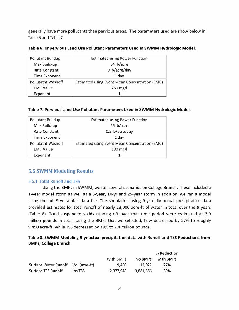
64

generally have more pollutants than pervious areas. The parameters used are show below in

Table 6 and Table 7.

Table 6. Impervious Land Use Pollutant Parameters Used in SWMM Hydrologic Model.

Pollutant Buildup Estimated using Power Function

Max Build-up 54 lb/acre

Rate Constant 9 lb/acre/day

Time Exponent 1 day

Pollutatnt Washoff Estimated using Event Mean Concentration (EMC)

EMC Value 250 mg/l

Exponent 1

Table 7. Pervious Land Use Pollutant Parameters Used in SWMM Hydrologic Model.

Pollutant Buildup Estimated using Power Function

Max Build-up 25 lb/acre

Rate Constant 0.5 lb/acre/day

Time Exponent 1 day

Pollutatnt Washoff Estimated using Event Mean Concentration (EMC)

EMC Value 100 mg/l

Exponent 1

5.5 SWMM Modeling Results

5.5.1 Total Runoff and TSS

Using the BMPs in SWMM, we ran several scenarios on College Branch. These included a

1-year model storm as well as a 5-year, 10-yr and 25-year storm In addition, we ran a model

using the full 9-yr rainfall data file. The simulation using 9-yr daily actual precipitation data

provided estimates for total runoff of nearly 13,000 acre-ft of water in total over the 9 years

(Table 8). Total suspended solids running off over that time period were estimated at 3.9

million pounds in total. Using the BMPs that we selected, flow decreased by 27% to roughly

9,450 acre-ft, while TSS decreased by 39% to 2.4 million pounds.

Table 8. SWMM Modeling 9-yr actual precipitation data with Runoff and TSS Reductions from BMPs, College Branch.

% Reduction

With BMPs No BMPs with BMPs

Surface Water Runoff Vol (acre-ft) 9,450 12,922 27%

Surface TSS Runoff lbs TSS 2,377,948 3,881,566 39%

65

5.5.2 Model Storm Runoff and TSS

The model storm events showed lower reductions in water runoff using BMPs than over

the whole time period. This is not surprising, given that once BMPs reach a capacity for

stormwater volume, they overflow or bypass the BMP and move downstream. Therefore, the

more intense the storm event, the lower % reduction the BMPs had. BMPs are generally

designed to reduce impacts from small storm events, rather than the largest, less frequent

storm events, thus this result is not surprising. TSS reduction using BMPs resulted in roughly

50% removal for each model storm event, while over the 9-yr period, the reduction was 39%. It

is unclear what is driving the differences between the storm events as TSS removal does not

appear to change in a linear direction, based upon the frequency of the storm. The difference in

the individual storms vs the 9-yr total (~50% vs ~40%) is not surprising due do different input

parameters. The 9-yr daily model uses a TSS buildup function, such that sediment builds up

over time, until it reaches capacity, or is washed off by precipitation. The model storm events

use a specific TSS buildup prior to the storm that may or may not be what happens in reality.

Therefore, one should look at these numbers as directionally correct, and focus more closely on

the total potential reductions over time.

Table 9. SWMM Model Stormwater Runoff and TSS Reductions from Current, using BMPs in College Branch.

The SWMM Model shows the potential for reductions in peak flows as well as total

flows in the system. As stated above, there is greater reduction under less intense storms, due

to the capacity of the BMPs (Table 10). BMPs show a reduction of peak flows by 29% for a 1yr

storm event down to a 10% reduction during a 25yr event. See Appendix C for idealized charts

of these storm events with and without BMPs. This model is somewhat crude, in that we do not

have routing from one BMP to the next. Routing goes directly from the subwatershed directly

to the outlet, or from the subwatershed to the bmp directly to the outlet. Therefore peakflows

are higher than what we would actually expect. Nevertheless, we should expect the relative

values of with and without BMPS to be generally correct. We may infact expect to get more

% Reduction From Current Using BMPs

Storm Event Total Precip (ac-ft) Water Runoff TSS

1yr 152 19% 48%

5yr 238 13% 58%

10yr 272 11% 56%

25yr 316 9% 55%

Total over 9 years 19,785 27% 39%

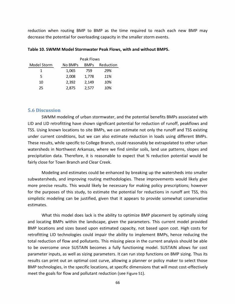
66

reduction when routing BMP to BMP as the time required to reach each new BMP may

decrease the potential for overloading capacity in the smaller storm events.

Table 10. SWMM Model Stormwater Peak Flows, with and without BMPS.

5.6 Discussion

SWMM modeling of urban stormwater, and the potential benefits BMPs associated with

LID and LID retrofitting have shown significant potential for reduction of runoff, peakflows and

TSS. Using known locations to site BMPs, we can estimate not only the runoff and TSS existing

under current conditions, but we can also estimate reduction in loads using different BMPs.

These results, while specific to College Branch, could reasonably be extrapolated to other urban

watersheds in Northwest Arkansas, where we find similar soils, land use patterns, slopes and

precipitation data. Therefore, it is reasonable to expect that % reduction potential would be

fairly close for Town Branch and Clear Creek.

Modeling and estimates could be enhanced by breaking up the watersheds into smaller

subwatersheds, and improving routing methodologies. These improvements would likely give

more precise results. This would likely be necessary for making policy prescriptions; however

for the purposes of this study, to estimate the potential for reductions in runoff ant TSS, this

simplistic modeling can be justified, given that it appears to provide somewhat conservative

estimates.

What this model does lack is the ability to optimize BMP placement by optimally sizing

and locating BMPs within the landscape, given the parameters. This current model provided

BMP locations and sizes based upon estimated capacity, not based upon cost. High costs for

retrofitting LID technologies could impair the ability to implement BMPs, hence reducing the

total reduction of flow and pollutants. This missing piece in the current analysis should be able

to be overcome once SUSTAIN becomes a fully functioning model. SUSTAIN allows for cost

parameter inputs, as well as sizing parameters. It can run step functions on BMP sizing. Thus its

results can print out an optimal cost curve, allowing a planner or policy maker to select those

BMP technologies, in the specific locations, at specific dimensions that will most cost-effectively

meet the goals for flow and pollutant reduction (see Figure 51).

Peak Flows Total Flows

Model Storm No BMPs BMPs Reduction

1 1,065 759 29%

5 2,008 1,778 11%

10 2,392 2,149 10%

25 2,875 2,577 10%

67

While this study looks at the potential for retrofitting LID technologies to an urban

landscape, it should be noted that often retrofitting can be significantly more expensive than

implementing BMPs as development occurs. Therefore, this method might be a worthwhile

step in planning in advance for new neighborhood and urban development, in addition to

retrofitting.

5.7 References Egodawatta, P. & Goonetilleke, A. 2006. Characteristics of Pollution Build-Up on Residential

Road Surfaces. Presented at the 7th International Conference on Hydroscience and Engineering

(ICHE 2006)

Lucas, W.C. 2004. Green Technology: The Deleware Urban Runoff Management Approach: A

Technical Manual for Designing Nonstructural BMPs to Minimize Stormwater Impacts from

Land Development. Deleware Department of Natural Resources and Environmental Control.

Rawls, W.J., D.L. Brakensiek, and N. Miller. (1983). Green-Ampt infiltration parameters from

soils data. Journal of Hydraulic Engineering 109(1):62–70.

Rossman, L.A. 2005. Stormwater Management Model Users Manual, Version 5.0. EPA/600/R-

05/040. U.S. Environmental Protection Agency, Water Supply and Water Resources Division,

National Risk Management Research Laboratory, Cincinnati, OH.

USEPA. 1999. Storm Water Technology Fact Sheet: Bioretention. Washington DC. EPA-832-F-

99-012

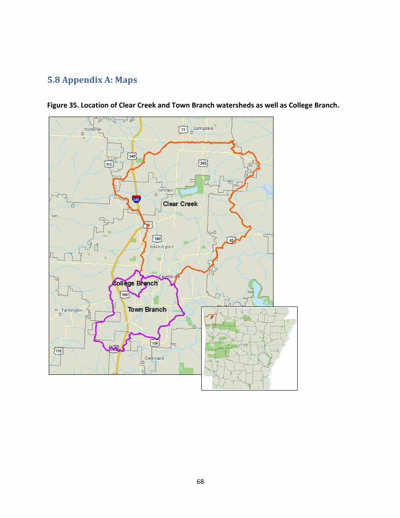
68

5.8 Appendix A: Maps

Figure 35. Location of Clear Creek and Town Branch watersheds as well as College Branch.

69

Figure 36. Clear Creek and Town Branch Soil Drainage.

70

Figure 37. Clear Creek and Town Branch Soil Hydrologic Group.

71

Figure 38. Clear Creek and Town Branch Topography.

72

Figure 39. Clear Creek and Town Branch Land Use.

73

Figure 40. Clear Creek and Town Branch BMP Siting using SUSTAIN.

74

Figure 41. College Branch selected subcatchments and BMP locations.

75

Figure 42. College Branch Land Use.

76

Figure 43. College Branch Topography.

77

Figure 44. College Branch Storm System Network.

78

Figure 45. College Branch BMP siting potential using SUSTAIN.

79

Figure 46. College Branch selected subcatchment and BMP locations.

Figure 47. College Branch subwatersheds and BMPs Modeled in SWMM.

80

Figure 48. College Branch 3D rendering of Buildings, subcatchments, BMPs, and storm system network.

Source: Google Earth Imagery

81

Figure 49. 3D Rendering of Buildings, Impervious Subwatersheds and BMPS.

Figure 50. Street Level View of Buildings and BMPs, College Branch.

Source: Google Earth Imagery

82

Figure 51. SUSTAIN Sample Output for Cost Effectiveness Curve for BMPs showing potential capabilities of SUSTAIN.

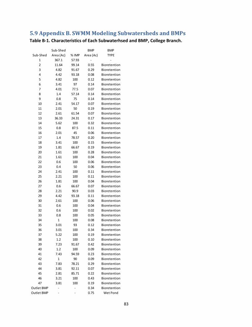
83

5.9 Appendix B. SWMM Modeling Subwatersheds and BMPs Table B-1. Characteristics of Each Subwaterhsed and BMP, College Branch.

Sub-Shed BMP BMP

Sub-Shed Area (Ac) % IMP Area (Ac) TYPE

1 367.1 57.93 - -

2 11.64 99.14 0.55 Bioretention

3 4.82 91.67 0.29 Bioretention


5 4.82 100 0.12 Bioretention





10 2.41 54.17 0.07 Bioretention


12 2.61 61.54 0.07 Bioretention

13 36.33 24.31 0.17 Bioretention






19 1.81 66.67 0.19 Bioretention










29 4.42 93.18 0.11 Bioretention





34 1 100 0.08 Bioretention





39 7.23 91.67 0.42 Bioretention


41 7.43 94.59 0.23 Bioretention

42 1 90 0.09 Bioretention

43 7.83 78.21 0.29 Bioretention

44 3.81 92.11 0.07 Bioretention

45 2.81 85.71 0.22 Bioretention



Outlet BMP - - 0.34 Bioretention

Outlet BMP - - 0.75 Wet Pond

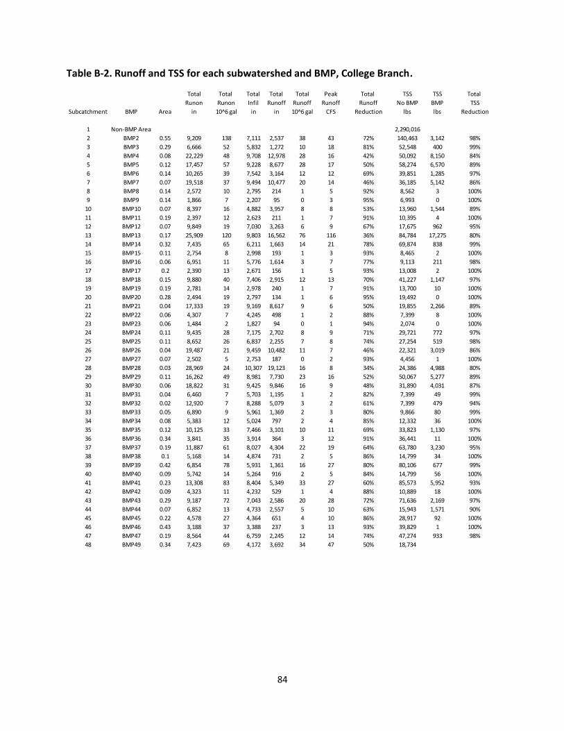
84

Table B-2. Runoff and TSS for each subwatershed and BMP, College Branch.

Total Total Total Total Total Peak Total TSS TSS Total

Runon Runon Infil Runoff Runoff Runoff Runoff No BMP BMP TSS

Subcatchment BMP Area in 10^6 gal in in 10^6 gal CFS Reduction lbs lbs Reduction

1 Non-BMP Area 2,290,016

2 BMP2 0.55 9,209 138 7,111 2,537 38 43 72% 140,463 3,142 98%

3 BMP3 0.29 6,666 52 5,832 1,272 10 18 81% 52,548 400 99%

4 BMP4 0.08 22,229 48 9,708 12,978 28 16 42% 50,092 8,150 84%

5 BMP5 0.12 17,457 57 9,228 8,677 28 17 50% 58,274 6,570 89%

6 BMP6 0.14 10,265 39 7,542 3,164 12 12 69% 39,851 1,285 97%

7 BMP7 0.07 19,518 37 9,494 10,477 20 14 46% 36,185 5,142 86%

8 BMP8 0.14 2,572 10 2,795 214 1 5 92% 8,562 3 100%

9 BMP9 0.14 1,866 7 2,207 95 0 3 95% 6,993 0 100%

10 BMP10 0.07 8,397 16 4,882 3,957 8 8 53% 13,960 1,544 89%

11 BMP11 0.19 2,397 12 2,623 211 1 7 91% 10,395 4 100%

12 BMP12 0.07 9,849 19 7,030 3,263 6 9 67% 17,675 962 95%

13 BMP13 0.17 25,909 120 9,803 16,562 76 116 36% 84,784 17,275 80%

14 BMP14 0.32 7,435 65 6,211 1,663 14 21 78% 69,874 838 99%

15 BMP15 0.11 2,754 8 2,998 193 1 3 93% 8,465 2 100%

16 BMP16 0.06 6,951 11 5,776 1,614 3 7 77% 9,113 211 98%

17 BMP17 0.2 2,390 13 2,671 156 1 5 93% 13,008 2 100%

18 BMP18 0.15 9,880 40 7,406 2,915 12 13 70% 41,227 1,147 97%

19 BMP19 0.19 2,781 14 2,978 240 1 7 91% 13,700 10 100%

20 BMP20 0.28 2,494 19 2,797 134 1 6 95% 19,492 0 100%

21 BMP21 0.04 17,333 19 9,169 8,617 9 6 50% 19,855 2,266 89%

22 BMP22 0.06 4,307 7 4,245 498 1 2 88% 7,399 8 100%

23 BMP23 0.06 1,484 2 1,827 94 0 1 94% 2,074 0 100%

24 BMP24 0.11 9,435 28 7,175 2,702 8 9 71% 29,721 772 97%

25 BMP25 0.11 8,652 26 6,837 2,255 7 8 74% 27,254 519 98%

26 BMP26 0.04 19,487 21 9,459 10,482 11 7 46% 22,321 3,019 86%

27 BMP27 0.07 2,502 5 2,753 187 0 2 93% 4,456 1 100%

28 BMP28 0.03 28,969 24 10,307 19,123 16 8 34% 24,386 4,988 80%

29 BMP29 0.11 16,262 49 8,981 7,730 23 16 52% 50,067 5,277 89%

30 BMP30 0.06 18,822 31 9,425 9,846 16 9 48% 31,890 4,031 87%

31 BMP31 0.04 6,460 7 5,703 1,195 1 2 82% 7,399 49 99%

32 BMP32 0.02 12,920 7 8,288 5,079 3 2 61% 7,399 479 94%

33 BMP33 0.05 6,890 9 5,961 1,369 2 3 80% 9,866 80 99%

34 BMP34 0.08 5,383 12 5,024 797 2 4 85% 12,332 36 100%

35 BMP35 0.12 10,125 33 7,466 3,101 10 11 69% 33,823 1,130 97%

36 BMP36 0.34 3,841 35 3,914 364 3 12 91% 36,441 11 100%

37 BMP37 0.19 11,887 61 8,027 4,304 22 19 64% 63,780 3,230 95%

38 BMP38 0.1 5,168 14 4,874 731 2 5 86% 14,799 34 100%

39 BMP39 0.42 6,854 78 5,931 1,361 16 27 80% 80,106 677 99%

40 BMP40 0.09 5,742 14 5,264 916 2 5 84% 14,799 56 100%

41 BMP41 0.23 13,308 83 8,404 5,349 33 27 60% 85,573 5,952 93%

42 BMP42 0.09 4,323 11 4,232 529 1 4 88% 10,889 18 100%

43 BMP43 0.29 9,187 72 7,043 2,586 20 28 72% 71,636 2,169 97%

44 BMP44 0.07 6,852 13 4,733 2,557 5 10 63% 15,943 1,571 90%

45 BMP45 0.22 4,578 27 4,364 651 4 10 86% 28,917 92 100%

46 BMP46 0.43 3,188 37 3,388 237 3 13 93% 39,829 1 100%

47 BMP47 0.19 8,564 44 6,759 2,245 12 14 74% 47,274 933 98%

48 BMP49 0.34 7,423 69 4,172 3,692 34 47 50% 18,734

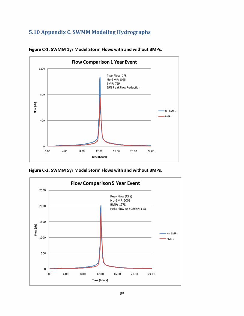
85

5.10 Appendix C. SWMM Modeling Hydrographs

Figure C-1. SWMM 1yr Model Storm Flows with and without BMPs.


0

400

800

1200

0.00 4.00 8.00 12.00 16.00 20.00 24.00

Flo

w (

cfs)

Time (hours)

Flow Comparison 1 Year Event

No BMPs

BMPs

Peak Flow (CFS)No-BMP: 1065 BMP: 75929% Peak Flow Reduction

0

500

1000

1500

2000

2500

0.00 4.00 8.00 12.00 16.00 20.00 24.00

Flo

w (

cfs)

Time (hours)


No BMPs

BMPs

Peak Flow (CFS)No-BMP: 2008BMP: 1778Peak Flow Reduction: 11%

86



0

500

1000

1500

2000

2500

0.00 4.00 8.00 12.00 16.00 20.00 24.00

Flo

w (

cfs)

Time (hours)


No BMPs

BMPs

0

1000

2000

3000

0.00 4.00 8.00 12.00 16.00 20.00 24.00

Flo

w (

cfs)

Time (hours)


No BMPs

BMPs

Peak Flow (CFS)No-BMP: 2392BMP: 2149Peak Flow Reduction: 10%

low impact development manual for arkansas

Documents