low-latency f0 estimation for the finger plucked electric

Revista de Informatica Teorica e Aplicada - RITA - ISSN 2175-2745Vol. 27, Num. 04 (2020) 79-94

RESEARCH ARTICLE

Low-Latency f0 Estimation for the Finger Plucked ElectricBass Guitar Using the Absolute Difference FunctionEstimador de f0 de Baixa Latencia para o Contrabaixo Eletrico Tocado com os DedosUsando a Funcao de Diferenca Absoluta

Christhian Fonseca1,2*, Tiago Tavares1,2

Abstract: Audio-to-MIDI conversion can be used to allow digital musical control through an analog instrument.Audio-to-MIDI converters rely on fundamental frequency estimators that are usually restricted to a minimumdelay of two fundamental periods. This delay is perceptible for the case of bass notes. In this dissertation, wepropose a low-latency fundamental frequency estimation method that relies on specific characteristics of theelectric bass guitar. By means of physical modeling and signal acquisition, we show that the assumptionsof this method are based on the generalization of all electric basses. We evaluated our method in a datasetwith musical notes played by diverse bassists. Results show that our method outperforms the Yin method inlow-latency settings, which indicates its suitability for low-latency audio-to-MIDI conversion of the electric basssound.Keywords: Fundamental frequency estimation — Low latency — Audio-to-MIDI converter — Music informationretrieval — MIDI-bass

Resumo: A conversao de audio para MIDI pode ser usada para permitir o controle musical digital por meiode um instrumento analogico. Os conversores de audio para MIDI dependem de estimadores de frequenciafundamental que sao frequentemente restritos a um atraso mınimo de dois perıodos da frequencia fundamental.Este atraso e perceptıvel no caso de notas graves, pois as frequencias fundamentais tem perıodos mais longos.Nesta dissertacao, propoe-se um metodo de estimativa da frequencia fundamental de baixa latencia que sebaseia em caracterısticas especıficas do baixo eletrico. Por meio de modelagem fısica e aquisicao de sinais,mostramos que o metodo se baseia na generalizacao para todos os baixos eletricos. Avaliamos nosso metodoem um conjunto de dados com notas musicais tocadas por diversos baixistas. Os resultados mostram que nossometodo supera o metodo Yin em configuracoes de baixa latencia, o que indica sua adequacao a conversao debaixa latencia de audio em MIDI do som de baixo eletrico.Palavras-Chave: Estimador de frequencia fundamental — Conversor de audio para MIDI de baixa latencia —Recuperacao de informacoes musicais — Baixo MIDI

1School of Electric and Computer Engineering (FEEC), University of Campinas, Brazil2Interdisciplinary Nucleus for Sound Studies (NICS), University of Campinas, Brazil*Corresponding author: christian [email protected]: http://dx.doi.org/10.22456/2175-2745.103182 • Received: 19/05/2020 • Accepted: 05/09/2020CC BY-NC-ND 4.0 - This work is licensed under a Creative Commons Attribution-NonCommercial-NoDerivatives 4.0 International License.

1. Introduction

Digital instruments and controllers commonly use communi-cation protocols such as the MIDI (Musical Instrument DigitalInterface) standard to communicate with each other. This al-lows combining different digital synthesizers, controllers, andeffect racks, which expands the expressive possibilities relatedto timbres, musical performances, musical recordings, and no-tations [1]. This toolchain can also include analog instrumentsby means of audio-to-MIDI converters [2].

Audio-to-MIDI converters are devices that aim at identify-

ing the notes played by an instrument in real-time or retrievingthem from an audio file. For such, they use a perceptual modelthat relates the fundamental frequency (f0) of an audio signalof a tonal sound to its pitch [3]. Many well-known algorithmsaim at estimating f0, such as the autocorrelation [4] and theYin method [5].

f0 estimators commonly aim at finding periodicity in asignal s j. The periodicity is based on the model

st = st+kT0 , (1)

where T0 is the fundamental period of st and k ∈ Z. Methods

Low Latency f0 Estimator for the Electric Bass Guitar

that rely on this property commonly require analyzing at leasttwo fundamental periods of the signal. This incurs in a lower-bound for the latency of Audio-to-MIDI conversion that canbe close to 50 ms for the lowest notes (41.2 Hz) in standard4-string electric basses. These long delays are perceptuallydetectable and this can impair the use of basses as a MIDIcontroller.

In this work, we aimed at attenuating this problem usingan f0 estimation method especially crafted for the electric bassguitar. The method exploits specific properties of the electricbass guitar waveform. Our method allows f0 estimation withan algorithmic latency of 1.1 times the fundamental period ofthe signal, which is about 27 ms for the lowest frequency noteof the four-string traditional bass guitar.

Experimental results show that this method is effectivewith an error rate of 15%. This is half the error rate of Yin, thebaseline method, when an equal latency is considered. Themethod was tested for the frequency range from 41.2 Hz to392 Hz, that is, from the lowest to the highest note of thestandard four-string electric bass guitar.

1.1 Pitch theoryPitch is a psychoacoustical atribute of the sound given by theauditory sensation often related to the perception of a repeti-tion rate of a waveform [6] above 20 Hz, where it is perceivednot as rhythm but as tone. The lowest regular repetition rateis called Fundamental Frequency (f0) and can be used to de-compose harmonic complex tones into sinusoidal harmoniccomponents whose frequencies are multiple integers of thefundamental frequency f0, that is:

st =M

∑m=1

am cos(2πm f0t +φm). (2)

The relative harmonic amplitudes am, among other atributes,are commonly associated to timbre differences and the funda-mental frequency f0 is closely related to the sensation of pitch[7]. In this study, we assume that the fundamental frequencyis the physical counterpart of the psychological sensation oftonality, commonly named as pitch, hence estimating the fun-damental frequency is equivalent to finding the pitch of asignal.

Moreover, perfectly periodic waveforms are rare, becausein the real world the signals differ between each repetition,even if small. Thus it is interesting to extend the conceptof pitch to quasi-periodic signals, that is, waveforms thatare not perfectly identical in each cycle, but have reasonablesimilarities between them to the point where they can beidentified as repetitions. Within this concept, the signals canbe modulated, turned off and on and yet have a pitch. Still,there are exceptions to pitch determination by fundamentalfrequency such as non-periodic but pitch-evoking signals [5].

The human ability to detect the pitch of a sound, that is,human tonal perception, has been linked to biological traitssuch as the periodicity of neural patterns [8] and the harmonicpartial pattern present by the cochlea [9]. Tonal perception

allows us to perceive the amount of repetition of events thatare too fast to be counted [10].

In music there are several standards that define the tuningfrequency for each note. The most commonly used nowadaysis called Pitch International Standard, which defines the fun-damental frequency of the note A above middle C should be440 Hz [11].

For the western music, in the equal tempered chromaticsystem, the frequency variation between one note and the nextis 2

112 and the variation given an interval ∆notes of notes is

given by the equation [12]:

∆ f req = f12∆notes

12 (3)

where f1 is the frequency of the lower note in the interval.

2. Related workThere are several methods that aim at finding the pitch ofperiodic signals such as Maximum likelihood [13], Spectralpeak picking [14], Cepstrum [15], Harmonic Product e SumSpectrum [13]. Two of them, Autocorrelation and Yin Method,were implemented and applied to a reference signal, whichis shown in Figure 1, of an excerpt from a recording of anelectric bass playing the note E0, which has approximately afundamental frequency of 41, 2Hz and a fundamental periodof 24.3 milliseconds.

Figure 1. Waveform from a electric bass guitar’s recordedsignal. f0 = 44.1Hz and T0 = 24.2ms. Its used as referencesignal for the application of the following pitch detectionmethods.

2.1 AutocorrelationIt is possible to measure the similarity between two signalsusing the correlation function, which compares and deter-mines the similarity of two waveforms at different intervals. Itpresents a function that shows how similar two similar signalsare for different intervals between the start of the two wave-forms. Autocorrelation is the application of the correlation

R. Inform. Teor. Apl. (Online) • Porto Alegre • V. 27 • N. 4 • p.80/94 • 2020


between a waveform and itself and is defined by the followingequation:

rt(τ) =t+WL

∑n=t+1

snsn+τ (4)

The autocorrelation rt(τ) is a measure of the similaritybetween the signal sn and a temporally shifted version sn+τ ofitself analyzed over a window with length WL.

A common method for estimating pitch of periodic signalsis by detecting the greatest positive peak of the autocorrela-tion function rt [4], as it presents peaks in values of τ thatcorrespond to the fundamental periods of sn. The fundamentalfrequency f0 is calculated by:

f0 =1

τmax,τ > 0, (5)

tal que:

rt(τmax) = maxrt(τ) (6)

The autocorrelation function, when applied to a periodicwaveform, is also periodic, showing maxima when the timelag τ is equal to or multiple of the fundamental signal periodand minimums when it is close to half of the period, as canbe seen in Figure 2, which shows the autocorrelation functionobtained from the reference signal, shown in Figure 1.

Figure 2. Autocorrelation function calculated from thewaveform in Figure 1. First peak after the initial one occursnear 24.2ms, as expected.

2.2 Yin methodAutocorrelation, presented earlier, commonly peaks not onlywith each waveform repetition but also due to the harmonicspresent in the signal. This creates difficulties for fundamentalfrequency estimators that use autocorrelation, as they areeventually unable to determine if a peak is relative to thefundamental frequency or signal harmonics.

The Yin method was proposed by Cheveigne and Kawa-hara. It is based on the same assumptions as of the autocorrela-tion method, with the addition of a series of modifications that

reduce errors. The name of the method (Yin) alludes to the Yinand Yang of Eastern philosophy, alluding to the search for thebalance between autocorrelation and cancellation proposedby the method to reduce errors.

The method consists in the application of 6 steps thatreduce the error rate in the fundamental frequency estimation[5]. Next, we briefly describe the improvements applied toeach step according to the authors’ study information.

2.2.1 Step 1: The autocorrelation methodIn the first step, the method uses autocorrelation, presented inthe previous subsection, obtaining an error rate of 10 % in theestimate of f0 when applied to the database presented in thestudy of its authors. As shown in the next steps, autocorrela-tion will no longer be used by the method.

2.2.2 Step 2: Difference functionIn the second step of the method, the autocorrelation func-tion is replaced by the difference function, reducing the errorrate to 1.95%. Here the period is no longer defined by thelargest peak, but by the largest dip in the function. A pos-sible cause for this reduction would be the high sensitivityof autocorrelation to amplitude changes, so that, increasesin signal amplitude lead the method to choose correlationfunction peaks from harmonics rather than fundamental ones.Figure 3 presents the difference function calculated from thewaveform of Figure 1. The difference function is defined bythe equation:

dt(τ) =WL

∑n=1

(sn− sn+τ)2. (7)

where sn is the input signal and sn+τ a τ samples shiftedversion of itself analyzed over a window with length WL.

Figure 3. Difference function calculated from the waveformin Figure 1. First big dip after the initial one occurs near 24.2ms, as expected.

2.2.3 Step 3: Cumulative mean normalized difference func-tion (CMNDF)

In the third step, the difference function is replaced by thecumulative mean normalized difference function reducing the



error rate a little more. As can be seen in Figure 4, unlikethe difference function, which starts at 0, the (CMNDF) startsat 1, eliminating the need for an upper frequency limit. Thislimit is required when the difference function is used, so thatthe first dip does not be selected as the fundamental frequencydip. The (CMNDF) is defined by:

d′t (τ) =

1 , if τ = 0

dt(τ)

(1/τ)τ

∑n=1

dt(n),otherwise

(8)

where dt(τ) is the diference function defined in equation (7)and τ the lag in samples between the signal and the shiftedversion of itself in diference function.

Figure 4. Cumulative mean normalized difference functioncalculated (CMNDF) from the waveform in Figure 1 and anabsolute threshold on dashed line. First big dip occurs near24.2 ms, as expected.

2.2.4 Step 4: Absolute thresholdThe fourth step is the use of an absolute threshold that de-creases by approximately half the error rate obtained in theprevious step, which generates a normalized function. ThisAbsolute threshold is represented by the dashed horizontalline in Figure 4. Using this threshold, dips above this valueare disregarded, avoiding the selection of harmonic generateddips.

2.2.5 Step 5: Parabolic interpolationIn the fifth step, a parabolic interpolation of the minimumlocation is included, but the reduction in the error rate isminimal. The idea is that this reduces the error when theperiod is not a multiple of the sampling period which couldlead to an error of up to half of the sampling period.

2.2.6 Step 6: Best local estimateIn the sixth step a new estimate is made, but now only inthe vicinity of the location indicated by the first estimate inorder to find the best local estimate. Seeking around 20%variation around the initial estimate, we obtained a reduction

of approximately 1/3 in the error rate compared to the previousstep.

Version Error rate (%)Step 1 10Step 2 1.95Step 3 1.69Step 4 0.78Step 5 0.77Step 6 0.50

Table 1. Error rates after application of each step of Yinmethod.

According to the study of Cheveigne and Kawahara (2002),the error rates obtained by the Yin method are about one-thirdtimes lower than the best competing methods, as evaluatedover a database of speech recorded together with a laryngo-graph signal. The error rates at each step are shown in table1.

2.3 Discussion about pitch estimation methodsMany methods, such as those discussed in the previous section,directly rely on the periodicity property as stated in Equation1 or the harmonic series model shown in Equation 2. Thisallows them to be applicable for the general case of findingpitch in periodic signals, but bounds them to a minimum delayof twice the fundamental period.

In this work, we propose a pitch detection method thatrelies on specific characteristics of the plucked electric bassstring. This restricts our method to signals generated by thisspecific instrument. However, it allows reducing the delay to1.1 times the fundamental period, which is very close to thetheoretical minimum latency.

This reduction is critical for real-time pitch detection inlower-pitch notes. In this range of notes, general-purposemethods require a delay of around 50ms to work properly.Our method allows detecting the same pitch with a delay ofaround 30ms.

The method proposed by [2] also indicates to estimate f0close to the theoretical minimum latency, i.e. the fundamentalperiod of the lowest observable pitch, but with higher compu-tational complexity, which can be problematic for embeddedreal-time applications, which can lead to an increase in delaydue to computational cost.

The proposed method is based on specific properties ofthe plucked electric bass signal. These properties are analyzedusing a physical model, which guides its generalization pos-sibilities. Then, the proposed model is compared to the Yinmethod using a dataset containing recordings from electricbass guitars.

For comparison purposes, the Yin method was chosenas the reference method. In addition to presenting excellentperformance as shown in [5] study, it is commonly used asa reference method, as in the study by [2], addressed in thiswork. It was also chosen because it is a well-known and citedmethod, as in the works of [16] and [17], also cited in this



work, counting more than 1300 citations according to theportal [18].

2.4 LatencyThe human perception of sounds is very sensitive to its tempo-ral characteristics. Therefore, audio delays are experienced inmany different scenarios and for many different reasons andis called latency. In the context of this work, the sound delayrefers to the time elapsed between an initial event, such asplaying a note on the electric bass guitar, for example, and asecond event, such as the moment when the sound is perceivedby a specific listener.

When you hear the sound from a sound source a fewmeters away, there is a delay due to the amount of time ittakes for this sound to travel through space over that distance.For example, in a room with a temperature of 20oC, the speedof sound is approximately 323.3 meters per second, whichcauses a delay of 2.91 milliseconds per meter of distancebetween the sound source and the listener. This delay or thedelay between two sound events can be large enough to benoticed and often causing several negative effects.

In music applications latency can be a very serious prob-lem as it directly impacts musicians’ performance in manyways, making it difficult to maintain steady tempo, rhythmicsynchronism between musicians and even tuning dependingon the instrument [19].

2.5 Causes for LatencyThere are many causes of unwanted delays. In orchestras, forexample, musicians on opposite sides can experience latenciesof up to 80 milliseconds due to the time it takes the soundto propagate through the distance between one musician andanother. Nowadays in most current performances, musiciansuse close speakers and headsets as feedback, most of thelatency comes from processing audio signals [19].

Digital processing of an instrument’s audio signal impliesa series of delays, starting with converting the analog to adigital signal at the system input and from digital to analogat the output. Buffering digital samples and phase delay ofdigital filters also add latency. Finally, the time required forprocessing the audio samples according to the applicationsused [20].

In the case of audio-to-midi converters, besides the timespent performing the algorithm operations to determine thefundamental frequency of the signal, there is still the necessaryinterval from the onset of a note played on the instrument forthe algorithm to estimate what is the fundamental frequency.Most f0 estimators need at least two periods to accomplish itstask.

2.6 Tolerable LatencyThe perception of how much a certain amount of latencybothers, hinders, or even precludes the correct use of the in-strument by the musician depends on the type of instrumentplayed and also on the musician’s listening skills. For exam-ple, musicians such as professional saxophonists are more

affected by latency and need more immediate feedback, con-sidering a latency of up to 10 milliseconds as acceptable, whilekeyboard players have a higher latency tolerance, consideringlatencies of up to 40.5 milliseconds as acceptable [21].

A previous study [21] has investigated the acceptable la-tency in live sound applications for different professional mu-sicians using in-ear monitoring (IEM) or wedge monitoring.The results of this study are presented in Table 2.

2.6.1 Latency DiscussionTable 2 shows that professional bassists consider a latencyof up to 30 milliseconds acceptable when using wedge mon-itoring. However, as already seen, most algorithms requirethe use of at least two periods to estimate f0, and the lowestnote of a traditional four-string bass, E0, has a period of 24.27milliseconds. That is, only the algorithmic delay for thesemethods is at least 2×24.27 = 48.54 milliseconds.

The method proposed in this study estimates the funda-mental frequency using a time interval of 1.1 times the period,starting from the note onset. For the same note E0, the al-gorithmic delay is 1.1×24.57 = 26.697 milliseconds, withinthe latency considered acceptable by professional bassists.

3. Methodology

3.1 Time-domain Behavior of a Plucked StringThis section discusses the properties of the plucked stringsignal that were used as a basis for our f0 estimation method.These properties were inferred by analyzing the audio signalof an electric bass string, as shown in Section 3.2, then thephysical model discussed in Section 3.3 was used to generalizethese results, as shown in Section 3.4.

3.2 Plucking an Electric Bass StringThe traditional electric bass guitar is an electro-acoustic in-strument with a body and neck made of wood and four metalstring tuned to E, A, G and D, which are fixed in a metalbridge on the body and in the nuts of the neck. The neckhas a fingerboard with 20 to 24 frets which divides it in tonalareas. The index and middle fingers of the right hand areused to pluck the strings and the fingertips of the left handare used to hold the strings against the fretted fingerboard.This changes the free length of the string, which modulatesits natural oscillation frequency.

There are magnetic pickups placed on the body of the in-strument, under the strings. They convert the string transversevelocity at its position into an electric voltage. The stringtransverse velocity can be seen as a wave that propagatesfrom the pluck position along the string length, reflecting andinverting when reaching the string end, as shown in Figure 5.

The waveform of the voltage signal at the pickups, asshown in Figure 8, indicates repetitions of a peak (positive ornegative) at the beginning of each cycle. In order to confirmthat this characteristic is maintained for all the electric bassguitars (instead of being a characteristic of the specific instru-



Latency (ms) Sax Vocals Guitar Drums Bass KeysIEM Good 0 1 4.5 8 4.5 27Wedge Good 1.5 10 6.5 9 8 22IEM Fair 3 6.5 14.5 54.5 25.5 46Wedge fair 10 26 16 25 30 40.5

Table 2. Tolerable latency - Instruments comparison using in ear monitoring (IEM) and wedge monitoring [21]

Figure 5. Position and velocity of a string along the x axis at different times t with fixed ends at x = 0 and x = L

ment), the behavior of its string was mathematically modeled,as discussed in the next section.

3.3 Physical modelThe behavior of the bass string can be modelled using an idealstring along the coordinate x with fixed ends at x = 0 andx = L with a transversal displacement along the coordinate y,which give us the following boundary conditions:

y(x = 0, t) = 0. (9)

y(x = L, t) = 0. (10)

The string has linear density µ and is stretched with aforce FT . It is initially at rest and is plucked in the positionx = xp with amplitude y(xp,0) = A as depicted in Figure 6. Inthis situation, the initial transverse displacement y(x,0) canbe expressed by

y(x, t = 0) =

{A( x

xp) , if x < xp

A(1− x−xpL−xp

) ,otherwise

}(11)

Figure 6. String with fixed ends at x = 0 and x = L beingplucked at x = xp with transversal displacement y(xp) = A.

Initially, the velocity distribution y′(0,x) is:

y′(x, t = 0) = 0. (12)

As depicted in Figure 7, for a short segment of this stringbetween x and ∆x there is a slope δy/δx = tan(θ) and avertical force F defined by:

F = FT sin(θ(x+∆x))−FT sin(θ(x)) (13)

If y corresponds to a small displacement, θ is also smalland can be approximated using sin(θ)≈ tan(θ) and tan(θ) =∂y∂x . This allows re-writing Equation (13) as:

F = FT (∂y∂x

(x+∆x)− ∂y∂x

(x)) (14)



Figure 7. Short segment of a string between (x,y) and(x+∆x,y+∆y) where a tension FT is applied.

Using the Newton’s second law:

F = m∂ 2y∂ t2 (15)

and knowing that the mass for this string segment is m = µ∆x,we have:

FT (∂y∂x

(x+∆x)− ∂y∂x

(x)) = µ∆x∂ 2y∂ t2 (16)

dividing both sides of Equation (16) by ∆x, applying thesecond derivative definition with ∆x −→ 0 and making c =√

FT/µ , it becomes the wave equation:

∂ 2y∂ t2 = c2 ∂ 2y

∂x2 , x ∈ (0,L), t ∈ (0, t f ] (17)

This model was used to simulate plucked strings and theresulting waveforms were compared to measured waveforms,as discussed in Section 3.4.

3.4 Plucked string simulationEquation 17 was numerically solved using the finite differencemethod [22] and the algorithmic steps used by Langtangen[23]. The Taylor series expansion was used to approximate itas:

y(x+∂x, t)−2y(x, t)+ y(x−∂x, t)∂x2 =

1c2

y(x, t +∂ t)−2y(x, t)+ y(x, t +∂ t)∂ t2

(18)

Using the i, j notation such that y(x, t) = yi j, inserting thewave number C = c∂ t

∂x and rearranging Equation 18 yields:

yi, j+1 =C2yi−1, j +2(1−C2)yi, j +C2yi+1, j−yi, j−1. (19)

To calculate the value of this function in the first time step,yi, j−1 must be determined. This can be done using the initialvelocity in Equation 12 and Tailor’s series as follows:

y(x, t +∂ t)− y(x, t−∂ t)2∂ t

= 0. (20)

Rearranging equation 20 and rewriting in the i, j notation,we find that:

yi, j−1 = yi, j+1. (21)

Finally, replacing yi, j−1 by yi, j+1 in Equation 19, isolatingyi, j−1 and dividing both sides by 2, we have:

yi, j+1 =C2

2yi−1, j +(1−C2)yi, j +

C2

2yi+1, j, (22)

which is the finite difference scheme. The numerical simu-lation was executed over the discrete spatial domain [0,L]equally spaced by ∂x and over the discrete temporal domain[0,T ] equally spaced by ∂ t.

The model’s pluck position xp = L/5 and the string lengthL = 0.87m were directly measured from the strings of anelectric bass. The wave velocity c was calculated using c =f/(2L) [12] related to note E0. The simulation time wasdefine as t f = 0.05s.

Over the spatial domain, the algorithm computes yi,0 usingEquation 11 and yi,1 using Equation 22 and applying theboundary conditions from Equations 9 and 10. Then, for eachelement j from temporal domain, apply Equation 19 to findyi, j+1 for each element i from the spatial domain, applyingthe boundary conditions again.

The output simulated signal was retrieved from the stringvelocity in the position x = L/5, approximately the pickupposition, and was yielded to a 5th order low-pass Butter-worth filter with a 150Hz cutoff frequency. This simulates thesmoother bend of the string due to its stiffness and the softtouch from the fingertip, which are responsible for generat-ing tones with weaker high-frequency components [24]. Theresulting signals were compared to the recorded signals, asshown in Figure 8.

Figure 8 shows that the physical model generates shapesthat are similar to those found in the acquired signals. Thismeans that the peak behavior is not a particular behavior ofthe specific electric basses that were used in our acquisitions.Rather, this behavior can be expected to appear in electricbasses in general, hence it can be used for further steps infundamental frequency estimation.

4. Fundamental Frequency EstimationThe simulated and measured waveforms in Figure 8 show thatthere is a peak at the onset of the note and at the beginningof each cycle after it. These peaks have approximately thesame width, regardless of the note’s frequency, and the note’sfundamental frequency occurs due to the rate in which peaksappear in the signal. The proposed method is based on thesetwo characteristics, as follows:

As it is a proposal for analysis in real-time, the signalcoming from the electric bass guitar must be analyzed contin-uously, that is, the analog electrical signal must be convertedto digital and the samples saved in a buffer for analysis. For



Figure 8. Simulated and measured notes played on string E of the electric bass guitar (a) E0 (b) A]0 (c) F1 (d) A1

each new sample obtained, the buffer must be updated, elimi-nating the “oldest” sample from it. A flowchart of the entirealgorithm process is presented in Figure 9.

4.1 Detect onsetInitially, it is necessary to detect the onset of the note that willbe played on the instrument. There are several methods fordetecting onsets that can be applied in this case, according tothe study by [25]. As in the case of the electric bass guitar,there is usually a rapid and considerable increase in relativeenergy when a note is played, it is proposed to use the methodbased on the energy function:

Enn =1

Nen

Nen

∑n=1|sn|2, (23)

where Nen is the length of the analysis window. A note onsetis detected when the energy variation is positive and biggerthan a threshold value.

4.2 Determine starting peakWhen onset is detected, the algorithm will seek to determinethe initial peak in the buffer, as expected according to figure10. The instant of occurrence of this peak is used to define thestart time of the short W -size integration window, also shownin Figure 10, which will be used in the following steps in theapplication of the absolute difference function.

4.3 Detect if there is enough dataThe W size of the short integration window is one of the inputparameters of the algorithm and must be less than half thewidth of the initial peak. Bearing in mind that for the same

string, the width of this peak remains approximately constant,regardless of the note.

To perform the next step, it is necessary to check if thenumber of samples available in the buffer generated after theinitial peak is greater than W , as an onset can be detected soquickly that the analyzed signal has not yet toured enough forthe generation of the samples necessary for the application ofthe absolute difference function.

4.4 Absolute difference functionThe next step is to apply the absolute difference function tothe W length section of the signal available in the buffer. Inthe initial instant, this signal will be exactly the same as theshort integration window itself, that is, the result will be zero.For each new sample that becomes available in the buffer,the absolute difference function is applied again, keeping thesame short integration window samples, but comparing it toa new signal segment, which contains the new sample madeavailable and does not contain the sample from the ”oldest”instant.

The absolute difference function is defined as:

d(τ) =W

∑n=1|sn− sn+τ |, (24)

where τ is the temporal lag between the initial peak and theanalized section from the audio signal sn. So we are measuringthe absolute difference between the first moments of the signalafter the initial peak in relation to the following sections ofthis same signal, resulting in a function like the one illustratedin Figure 11.



Figure 9. Proposed method flowchart process.

The absolute difference function must be applied to eachbuffer update until it has passed, from the initial peak, aninterval of 1.1 times the fundamental period T0 of the lowest

frequency to be detected. Theoretically, this interval couldbe T0 +W , but the first cycle from the onset is subject toharmonics that can vary the interval between the first two



Figure 10. Analyzed signal sn and integration short windowwith size W . This signal is a recording of the G0 note playedon the E string of an electric bass guitar

Figure 11. Absolute difference function from the analyzedsignal sn from figure 10 and threshold value represented asthe horizontal dotted line

peaks of the signal. Thus, 1.1×T0 gives a margin of tolerance.

4.5 Find local minimaIn sequence, the algorithm searches for local minima in theabsolute difference function, referenced as dips in Figure 11.For the lowest notes, there will be only a local minimumas depicted in Figure 11, from which we will obtain the τ0interval. For the highest notes, as exemplified in Figure 12,there may be 2 or 3 local minimums, as depicture in Figure13, depending on how many frets the bass has. In this case, τ0is obtained by:

τ0 =Nτ

∑n=1

τn

n, (25)

where Nτ is the number of local minimums and τn is the tem-poral lag between the initial peak and nTH local minimums.

4.6 Determine f0Since τ0 represents the interval in which the signal most seemsto repeat its initial stretch, we define that the fundamentalperiod of the T0 signal is equal to τ0. Thus we determine thefundamental frequency f0 of the signal as:

f0 =1T0

(26)

Therefore, briefly, the proposed method consists of theapplication of the signal to an absolute difference with a win-dow size W shorter than half-width of this first peak as shown

Figure 12. Analyzed signal sn and integration short windowwith size W . This signal is a recording of the G1 note playedon the E string of an electric bass guitar

Figure 13. Absolute difference function from the analyzedsignal sn from figure 12 and threshold value represented asthe horizontal dotted line

in Figure 10. This thin window plays an important role tomake it possible for the method to find f0 after 1.1 times thefundamental period, whereas the Yin method needs more thantwo fundamental periods [5], as shown in Figure 14.

5. Experiments and results

5.1 DatasetThe proposed method was tested using a set of audio record-ings acquired from 3 different electric bass guitars. Each ofthem was played by a different musician, and all of them usedthe finger-plucking technique. All notes within the instru-ment’s range were recorded from each of the guitars, usingtwo different instrument equalizations (full bass and full tre-ble). This yielded 528 recordings, which were all manuallycropped to start at the note onset since the proposed methoddoes not have a note onset detector.

5.2 ExperimentsThis section describes experiments that compare the proposedmethod to the Yin method [5], as implemented by Guyot[26]. The experiments comprised executing both the proposedmethod and the Yin method to estimate the f0 in the datasetsamples.

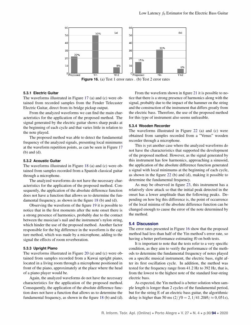
5.2.1 Test 1 - sample length for noteIn this first test, the sample length provided as input parame-ters for the algorithms is equal to 1.1×Tt1× f s, being Tt1 thefundamental period of the expected note and f s the sampling



Figure 14. Algorithmic delay for the proposed method and for the Yin method.

frequency of the digital audio signal. To serve as a reference,the test was repeated for the Yin method with a sample lengthequal to 2.1×Tt1× f s and is referenced as ”Yin2” in Figure16 (a).

5.2.2 Test 2 - sample length for stringThis second test is a more common application for a pitchdetector in a string instrument, where the fundamental fre-quency should be estimated from a range of approximately 2octaves. So, the sample length provided as input parametersfor the algorithms is equal to 1.1× Tt2× f s, being Tt2 thefundamental period of the lower note from the specific stringto which the recorded note belongs. Also, in this case, the testwas repeated for the Yin method with a sample length equalto 2.1×Tt2× f s and is referenced as ”Yin2” in Figure 16 (b).

Figure 15 compares the length of the samples used in test1, shown in the first column, and test 2, shown in the secondcolumn of the figure.

To determined if the method fails, the MIDI note corre-spondent to the fundamental frequency estimated is calculatedas:

Mnote = 12log(

f0

16.351597

)1

log(2), (27)

where f0 is the estimated fundamental frequency and 16.351597is the f0 for the MIDI note = 0. The result is rounded to thenearest integer. If the calculated MIDI note differs from theexpected one, it is counted as one error.

5.3 Proposed method applied to other musical in-struments

The proposed method was developed based on specific char-acteristics of the electric bass waveform when played usingthe finger plucking technique. These characteristics wereobserved in samples of recordings made with the referredinstrument and mathematically modeled to guarantee thatthey will be present in the waveforms generated by electricbasses in general. As these characteristics may be also presentin waveforms generated by other instruments, this section

Figure 15. sample lengths for test 1 in the first column andfor test 2 in the second column

presents the results of applying the method to audio samplesof some other instruments in order to indicate promising pathsfor future work in the expansion of the method application.

The samples of musical instruments analyzed below wereobtained from the soundbank of the FreePats project [27].



Figure 16. (a) Test 1 error rates . (b) Test 2 error rates

5.3.1 Electric GuitarThe waveforms illustrated in Figure 17 (a) and (c) were ob-tained from recorded samples from the Fender TelecasterElectric Guitar, direct from its bridge pickup output.

From the analyzed waveforms we can find the main char-acteristics for the application of the proposed method. Thesignal generated by the electric guitar shows sharp peaks atthe beginning of each cycle and that varies little in relation tothe note played.

The proposed method was able to detect the fundamentalfrequency of the analyzed signals, presenting local minimumsat the waveform repetition points, as can be seen in Figure 17(b) and (d).

5.3.2 Acoustic GuitarThe waveforms illustrated in Figure 18 (a) and (c) were ob-tained from samples recorded from a Spanish classical guitarthrough a microphone.

The analyzed waveforms do not have the necessary char-acteristics for the application of the proposed method. Con-sequently, the application of the absolute difference functiondoes not have a function that allows us to determine the fun-damental frequency, as shown in the figure 18 (b) and (d).

Observing the waveform of the figure 19 it is possible tonotice that in the first moments after the note onset there isa strong presence of harmonics, probably due to the contactbetween the musician’s nail and the instrument’s nylon string,which hinder the use of the proposed method. Another factorresponsible for the big difference in the waveform is the cap-ture method, which was made by a microphone, adding to thesignal the effects of room reverberation.

5.3.3 Upright PianoThe waveforms illustrated in Figure 20 (a) and (c) were ob-tained from samples recorded from a Kawai upright piano,located in a living room through a microphone positioned infront of the piano, approximately at the place where the headof a piano player would be.

Again, the analyzed waveforms do not have the necessarycharacteristics for the application of the proposed method.Consequently, the application of the absolute difference func-tion does not have a function that allows us to determine thefundamental frequency, as shown in the figure 18 (b) and (d).

From the waveform shown in figure 21 it is possible to no-tice that there is a strong presence of harmonics along with thesignal, probably due to the impact of the hammer on the stringand the construction of the instrument that differs greatly fromthe electric bass. Therefore, the use of the proposed methodfor this type of instrument also seems unfeasible.

5.3.4 Wooden RecorderThe waveforms illustrated in Figure 22 (a) and (c) wereobtained from samples recorded from a ”Venus” woodenrecorder through a microphone.

This is yet another case where the analyzed waveforms donot have the characteristics that supported the developmentof the proposed method. However, as the signal generated bythis instrument has few harmonics, approaching a sinusoid,the application of the absolute difference function generateda signal with local minimums at the beginning of each cycle,as shown in the figure 22 (b) and (d), making it possible todetermine the fundamental frequency.

As may be observed in figure 23, this instrument has arelatively slow attack so that the initial peak detected in theonset has a lower amplitude than the following peaks. De-pending on how big this difference is, the point of occurrenceof the local minima of the absolute difference function can bechanged enough to cause the error of the note determined bythe method.

5.4 DiscussionThe error rates presented in Figure 16 show that the proposedmethod had less than half of the Yin method’s error rate, sohaving a better performance estimating f0 on both tests.

It is important to note that the tests refer to a very specificcondition, as they aim to verify the performance of the meth-ods to determine the fundamental frequency of notes playedon a specific musical instrument, the electric bass, right af-ter its first oscillation cycle. In addition, the method wastested for the frequency range from 41.2 Hz to 392 Hz, that is,from the lowest to the highest note of the standard four-stringelectric bass.

As expected, the Yin method is a better solution when sam-ple length is longer than 2 cycles of the fundamental period,but for the string E of an electric bass guitar, the algorithmicdelay is higher than 50 ms (2/ f 0 = 2,1/41.20Hz≈ 0,051s),



Figure 17. Analyzed signals from an electric guitar: (a) note E1; (c) note E2. Absolute difference function: (b) from signal inFigure (a); (d) from signal in Figure (c).

Figure 18. Analyzed signals from an acoustic guitar: (a) note E1; (c) note E2. Absolute difference function: (b) from signal inFigure(a); (d) from signal in Figure (c).

Figure 19. Waveform from an acoustic guitar attack and first cycles.

which is perceptible for a bass player, making it harder toplay the bass guitar with real-time MIDI outputs, as shown in

the [21] study, where professional bassists deemed acceptablelatencies of up to 30 ms.



Figure 20. Analyzed signals from an Upright Piano: (a) note A0; (c) note A1. Absolute difference function: (b) from signal inFigure(a); (d) from signal in Figure (c).

Figure 21. Waveform from an Upright Piano attack and first cycles.

Figure 22. Analyzed signals from a wooden recorder: (a) note A5; (c) note A6. Absolute difference function: (b) from signal inFigure(a); (d) from signal in Figure (c).



Figure 23. Waveform from an wooden recorder attack and first cycles.

The study on the application of the proposed method toother musical instruments indicated that there is a possibil-ity of obtaining good results with the electric guitar. This isdue to the fact that the instruments share many constructivecharacteristics, such as metallic strings and capture by electro-magnetic pickups. For the acoustic guitar and upright piano,the results were not promising. The waveforms generated bythese instruments are quite different from those generated bythe electric bass, mainly because the sound generated is not asimple capture of the vibrating string, but rather the vibrationof its entire structure. Finally, the method even proved to bereasonably applicable to the Wooden Recorder, but as thisinstrument reproduces high notes, more accurate methods thatuse more than two cycles for the detection of the pitch willnot present great latencies.

6. ConclusionA method based on the absolute difference function and thewaveforms from a finger plucked strings of an electric bassguitar was presented. It was tested over 528 notes recordedfrom three different bass guitars and it shows to be capableto estimate these notes from samples with length equal to 1.1times their fundamental periods, while our reference method,Yin, under the same conditions, had double the error rate. Thisshorter algorithmic delay, near the minimal theoretical delay(one fundamental period) and low computational complexity,makes the proposed method suitable for real-time applicationsfor the electric bass guitar, such as a MIDI bass guitar.

However the method missed 15% of the notes on test 2,which is a similar application, so future studies should bemade to improve these results. An approach to reduce errors,unrelated to improvements in the method, would be to adopta specific way of playing the musical instrument. If the bassplayer always plucks the string smoothly, in order to keep thefirst cycles of the signal similar to the modeled ones, errorrates can be drastically improved. It can be a useful alternativeway to a MIDI bass guitar, where the way you pluck the stringswill not affect the sound timber. But, clearly, this imposesa limited way to play in exchange for a more precise notedetection and lower latency

Also, the method was not tested for notes played on topof an already vibrating string which certainly should make itharder to estimate the correct f0. However, it is possible thatcontact with the plucking finger, at the moment of playing thenew note, dampens the string enough to not interfere with the

performance of the method. This case will be approached infuture work.

The method is applicable for pitch determination for mono-phonic electric bass signals, so in a real application, it wouldbe necessary to use individual pickups per string, so that eachgenerated signal can be analyzed individually and ensuringthat there will be no more than one note simultaneously foreach signal. In addition, the method requires a quick onsetsdetector, which provides the information that a note has beenplayed to begin the analysis process.

A promising path for future work would be the develop-ment of a hybrid method, which uses the proposed method forrapid pitch detection in low notes and another more accuratemethod using at least two cycles, such as Yin, for higher notes.Thus, adjusting the proposed method to provide an estimateafter an analysis window of 1.1 times the period of the lowestfundamental frequency, and the second method to provide anestimate as soon as it is obtained, that is, after two cycles ofthe analyzed frequency, we will have the following process:if the note is high, the second method will offer the estimatebefore the end of the analysis of the proposed method, other-wise the proposed method will provide its estimate, avoidinggreater latencies.

Finally, future works can study how the use of the reed toplay the strings affects the error rates, which could allow theapplication of the method for the electric guitar, an instrumentthat indicated to have similar characteristics in the waveforms,from those used in the analysis by the proposed method.

7. Acknowledgements

Thanks are due to Mario Junior Patreze from ”Escola deMusica de Piracicaba Maestro Ernst Mahle”, Marcio H. Gold-schmidt and Giovani Guerra from musical studio ”Esgoto”for the records from their own electric bass guitars whichcompose the database of this work. This study was financedin part by the ”Coordenacao de Aperfeicoamento de Pessoalde Nıvel Superior” - Brasil (CAPES) - Finance Code 001.

Author contributionsChristhian Fonseca developed the study as his master’s re-search, supervised by Tiago Tavares.



References[1] GIBSON, J.; WARREN, A. The MIDI Standard.[S.l.]: http://www.indiana.edu/ emusic/361/midi.htm, ac-cessed 05/9/2019.

[2] DERRIEN, O. A very low latency pitch tracker for audioto midi conversion. 17th International Conference on DigitalAudio Effects (DAFx-14), 2014.

[3] KLAPURI, A. P. Multiple fundamental frequency esti-mation based on harmonicity and spectral smoothness. IEEETrans. Speech and Audio Proc, 2003.

[4] RABINER, L. On the use of autocorrelation analysis forpitch detection. IEEE Transactions on Acoustics, Speech, andSignal Processing, v. 25, n. 1, p. 24–33, February 1977.

[5] CHEVEIGNE, A. de; KAWAHARA, H. YIN, a funda-mental frequency estimator for speech and music. The Journalof the Acoustical Society of America, v. 111, n. 4, p. 1917–1930, 2002.

[6] HELLER, E. J. Why You Hear What You Hear. [S.l.]:Princeton University Press, 2012. (Chapter 23; pp. 437-504).

[7] OXENHAM, A. J. Pitch perception. Journal of Neuro-science, v. 32, n. 39, p. 13335–13338, 26 September 2012.

[8] CARIANI, P. A.; DELGUTTE, B. Neural correlates ofthe pitch of complex tones. I. Pitch and pitch salience. J.Neurophysiol. 76, 1996.

[9] TERHARDT, E. Pitch, consonance and harmony. J.Acoust. Soc. Am. 55, 1974.

[10] FORNARI, J. Percepcao, Cognicao e Afeto Musical.[S.l.: s.n.], 2010.

[11] ISO16:1975-ACOUSTICS. Standard tuning frequency.[S.l.]: International Organization for Standardization, 1975.

[12] IAZZETTA, F. Tutoriais de Audio e Acustica. [S.l.]:http://www2.eca.usp.br/prof/iazzetta/tutor/acustica, accessed04/25/2019.

[13] NOLL, A. M. Pitch determination of human speech bythe harmonic product spectrum, the harmonic surn spectrum,and a maximum likelihood estimate. Symposium on ComputerProcessing in Communication, ed., University of BroodlynPress, New York, v. 19, p. 779–797, 1970. Disponıvel em:〈https://ci.nii.ac.jp/naid/10000045637/en/〉.[14] OPPENHEIM, A.; SCHAFER, R. Discrete-Time Sig-nal Processing. [S.l.]: Prentice Hall, 1999. ISBN-10:0137549202.

[15] SINGH, C. P.; KUMAR, T. K. Efficient pitch detec-tion algorithms for pitched musical instrument sounds: Acomparative performance evaluation. In: 2014 InternationalConference on Advances in Computing, Communications andInformatics (ICACCI). [S.l.: s.n.], 2014. p. 1876–1880.

[16] GERHARD, D. Pitch extraction and fundamental fre-quency: History and current techniques. Technical ReportTR-CS 2003-06, 2003.

[17] KNESEBECK, A.; ZOLZER, U. Comparison of pitchtrackers for real-time guitar effects. 13th Int. Conference onDigital Audio Effects (DAFx-10), 2010.

[18] RESEARCHGATE. YIN, A fundamental fre-quency estimator for speech and music. [S.l.]:https://www.researchgate.net/publication/11367890 YINA fundamental frequency estimator for speech and music,accessed 06/02/2020.

[19] GREEF, W. The influence of perception latency on thequality of musical performance during a simulated delay sce-nario. University of Pretoria, Department of Music, 2016.

[20] WANG, Y. Low latency audio processing. Queen MaryUniversity of London, School of Electronic Engineering andComputer Science, 2017.

[21] LESTER, M.; BOLEY, J. The effects of latency on livesound monitoring. Journal of the Audio Engineering Society,2007.

[22] JAIN, M. Numerical Methods for Scientific and Engineer-ing Computation. 1st ed.. ed. [S.l.]: New Age International,2003. ISBN-10: 8122414613. pp: 844.

[23] LANGTANGEN, H. Finite difference methods for wavemotion. preliminary version. [S.l.]: Department of Informatics,University of Oslo, 2016.

[24] JANSSON, E. Acoustics for Violin and Guitar Makers.4th ed.. ed. [S.l.]: http://www.speech.kth.se/music/acviguit4/,2002. (Chapter 4; pp. 16-18).

[25] PORCIDES, C.; TAVARES, L. Resultados preliminaresde um estudo comparativo de metodos de deteccao de onsetsem sinais de Audio. Anais do Simposio de Processamento deSinais da UNICAMP, Vol. 1, 2014.

[26] GUYOT, P. Fast python implementation of the yin al-gorithm. http://doi.org/10.5281/zenodo.1220947, 2018. ”ac-cessed 01/02/2018”.

[27] FREEPATS. Sound Banks. [S.l.]:http://freepats.zenvoid.org/index.html, accessed 09/02/2020.


https://ci.nii.ac.jp/naid/10000045637/en/

low-latency f0 estimation for the finger plucked electric

Documents